Automatic Proof of Graph Nonisomorphism · For mathematical problems, ... operations. By counting, for each vertex, ... Automatic Proof of Graph Nonisomorphism 5Published in: Mathematics

Math.comput.sci. Online Firstc© 2008 Birkhauser Verlag Basel/Switzerland

DOI 10.1007/s11786-008-0052-8

Mathematics inComputer Science

Automatic Proof of Graph Nonisomorphism

Arjeh M. Cohen, Jan Willem Knopper and Scott H. Murray

Abstract. We describe automated methods for constructing nonisomorphismproofs for pairs of graphs. The proofs can be human-readable or machine-readable. We have developed an experimental implementation of an interac-tive webpage producing a proof of (non)isomorphism when given two graphs.

Mathematics Subject Classification (2000). 05C60, 68R10, 05C25, 03B35.

Keywords. Graphs, groups, graph isomorphism, automatic proof generation.

1. Introduction

With the growth in computer power and internet access, an increasing numberof problems are solved on remote machines by programs written by experts in aparticular field. In this situation, the user may have no knowledge of the algorithmused, its implementation, or indeed how the remote machine is maintained. A mereyes-or-no answer cannot be trusted; we need additional verification that the answeris correct. For mathematical problems, the most obvious form of verification is aproof of correctness.

In this article, we discuss the construction of proofs for the graph isomorphismproblem. Here a graph is understood to be a finite undirected graph without loops(i.e., edges having a single end point) and without multiple edges. If two graphs areisomorphic, and we are given an explicit isomorphism σ, then it is straightforwardto verify that σ is an isomorphism and hence that the graphs are isomorphic.Proving that a pair of graphs are not isomorphic is more difficult. We show howto generate such a proof automatically.

The proof produced by our software is human-readable but could be modifiedto give machine-readable proofs as in [6]. We use a lot of computer time to find ashort and understandable proof. Hence it can take much longer to generate a proofthan to determine nonisomorphism. We discuss an experimental implementationof an interactive webpage producing such a proof when given two graphs. Thisworks as a proof assistant in the sense that the author is able to choose optionsfor generating such a proof. At the same time, the key ingredients of our proof

2 A. M. Cohen et al. Math.comput.sci.

are machine-readable and so can be used to construct a formal proof. In thismanner, our work acts as an oracle providing the key data for a formal proof ofnonisomorphism for two given graphs. This can lead to the skeptical use of ouroutput by a proof checker in the terminology of [9] and [3]. Alternatively, it canbe seen as a little engine of proof in the terminology of [21].

The first step in finding a non-isomorphism proof consists of a search fordistinguishing invariants. An invariant is a function on graphs that takes thesame value on isomorphic graphs, but may take different values on nonisomor-phic graphs. In many cases, invariants give short and easy-to-verify proofs of non-isomorphism. For example, two graphs with different numbers of vertices clearlycannot be isomorphic, so the number of vertices is an easily-checked invariant.For a given input of two graphs, a distinguishing invariant is an invariant withdistinct values on the two graphs. When such an invariant is found (and provencorrect), the proof of nonisomorphism will be no longer than the evaluation of thisfunction on each graph. The invariants incorporated in our software are discussedin Section 2.

If no simple invariants can be found to distinguish two graphs, we resort togeneral graph-isomorphism algorithms building on the methods of [6]. We have im-plemented Luks’ algorithm [13], and modified it to output a human-readable proof.We have also modified the nauty implementation [14] of McKay’s algorithm [16] toproduce such a proof. In this paper we only discuss McKay’s algorithm, as it gavea shorter proof than Luks’ in every case we tried. Our modified version can alsoprove the correctness of the identification of the automorphism group of a graph.This is the content of Section 3.

We have developed an experimental proof constructor for graph nonisomor-phism [20]; it is described in Section 4. It will automatically construct a proof of(non)isomorphism. In addition, a user can compose a proof interactively by choos-ing invariants or calling one of the modified algorithms. The proof constructor,with installation instructions, can be found in the MathDox repository [20].

Although we do not focus on complexity in this paper, it may be worthmentioning that graph nonisomorphism is neither known nor believed to be in NP,that graph isomorphism has time complexity O(exp(n1/2+o(1))) (cf. [1, 13]), andthat graph nonisomorphism has subexponential size proofs unless the polynomial-time hierarchy collapses (cf. [12]), where n refers to the number of vertices of Gand subexponential is understood to mean O(exp(nε)) for every ε > 0. The proofsthat our program generates are not based on these advanced algorithms.

2. Invariants

As a first approach to finding a nonisomorphism proof for two given graphs, thefollowing 16 invariants are checked in order.

1. number of vertices2. number of edges3. degree multiset

Automatic Proof of Graph Nonisomorphism 3

4. diameter5. girth6. distance multiplicity7. local component number multiset8. extended local component number multiset9. characteristic polynomial of the adjacency matrix

10. Smith normal form of the adjacency matrix11. powers of the adjacency matrix12. multisets of numbers of triangles per vertex/edge13. multiset of numbers of K2,1,1-graphs per edge14. edge distance multiplicity15. multiset of all local K2,1,1-graph numbers16. multiset of all local adjacency matrix powers

Let G be a graph. The complexity of computing the invariants listed is mostfrequently expressed in n, the number of vertices of G, that is, invariant (1).Clearly, computation of the invariant (2), the number of edges, requires at most(n2

)operations. By counting, for each vertex, the number of edges on which it

lies, we find (3), the degree multiset {0, . . . , n − 1} → N (we use the convention0 ∈ N) that assigns to each possible degree the number of vertices of G havingthat degree. The distance in G is the function on pairs of vertices that gives theshortest length of a path from one vertex to the other; here, a path of length kfrom v to w is a sequence v0, v1, v2, . . . , vk of k + 1 vertices of G with vi adjacentto vi−1 for i ∈ {1, . . . , k} and v = v0, w = vk; if there is no such path from v to win G, the distance between v and w is set to ∞. Invariant (4), the diameter of G,is the largest distance realized in G.

Most of our algorithms assume that the graphs are connected , which meansthat the diameter is finite (see the text before the example of Section 4). Thelargest connected subgraphs of G are called connected components . The girth ofG, invariant (5), is the smallest positive length of a path from a vertex to itselfoccurring in G and without repeats and retreats (so vi−2 �= vi �= vi−1 for each iif the path is v = v0, v1, v2, . . . , vk = v); if there are no such paths, the graph is aunion of trees and the girth is set to ∞.

The distance multiplicity of a vertex is the multiset of distances between thevertex and all other vertices. The multiset of distance multiplicities of all vertices isthe distance multiplicity of the graph, invariant (6). The distance multiplicity of anedge is the multiset of distances between other vertices and a vertex of that edge.The edge distance multiplicity of a graph, invariant (14), is the multiset of distancemultiplicities of all edges. The subgraph induced on the set of vertices at distanceone from a vertex is called the neighbor graph of that vertex. The local componentnumber of a vertex is the multiset of the sizes of the connected components ofthis subgraph. The multiset of local component numbers of all vertices of G is thelocal component number multiset , invariant (7), of the graph. The extended local


component number multiset , invariant (8), is like the local component number,except now the vertices at distance i are used instead of those at distance 1 foreach distance i occurring in G.

The adjacency matrix A of G is an n×n matrix whose rows and columns areindexed by the vertices of G and in which all entries are 0 except those whose rowand column are indexed by vertices v and w, respectively, for which (v, w) is anedge of G; for these edges the entry is 1. In particular, the trace of the adjacencymatrix is equal to 0 and the (v, w)-entry (Ak)vw of its k-th power is nonzero if andonly if there is a path of length k from v to w. Since it takes O(n3) operations tocompute each power in turn, computing all distances requires at most O(n4) integeroperations. The set of powers of the adjacency matrix itself is not an invariant, butit can easily be turned into one: the multiset of multisets {((A1)vw, . . . , (An−1)vw) |w vertex of G} for v running over the vertices of G. This is invariant (11). Also, thecharacteristic polynomial of the adjacency matrix , invariant (9), can be computedin this time. The Smith normal form of the adjacency matrix , invariant (10), isstronger, i.e., distinguishes more graphs, than the rank of the adjacency modulo pfor any prime p; see [10] for its precise definition and efficient computation.

A path v, u, w, v in G of length 3 with u �= v �= w �= u is called a triangle of G.If G has a triangle, its girth is 3. Invariant (12), the multiset of numbers of trianglesper vertex, edge, counts the number of triangles on each vertex, respectively, edge.A subgraph of G on four vertices such that all unordered pairs except for one areedges is called a K2,1,1-graph. Its two vertices of degree 3 form an edge that we callits diagonal . Counting, for each edge of G, the number of K2,1,1-graphs having thatedge as its diagonal, we obtain invariant (13), the multiset of numbers of K2,1,1-graphs per edge. Invariant (15), the multiset of all local K2,1,1-graph numbers, isthe multiset of the values of invariant (13) for all neighbor graphs of vertices ofthe graph. Invariant (16), the multiset of all local adjacency matrix powers, is themultiset of the values of the invariant (11) for all neighbor graphs of vertices ofthe graph.

The order of the invariants is chosen to balance understandability with easeof calculation. In larger graphs some of the invariants further down the list becomeharder to verify by hand, but still can give information about the graph in poly-nomial time. In fact, all except invariants (10), (15), and (16) are O(n4), where nis the number of vertices of G, but some have a better exponent.

Note that some invariants are straightforward to calculate but harder to provecorrect. Some effort is made to reduce the output; for example if the number ofvertices with a certain degree differs in two graphs, it is not necessary to list thenumber of vertices with other (fixed) degrees.

3. McKay’s algorithm

The current implementation of McKay’s algorithm [15, 16], called nauty [14], isone of the most efficient practical graph isomorphism solvers available. We have


modified this program to give additional output, that allows us to construct ahuman-readable proof. In this section, we outline McKay’s program; in the nextsection, we will discuss our modifications.

Nauty’s default routine for establishing nonisomorphism involves computinga canonical labeling for each graph. That is, a labeling of the vertices by integerswith the property that two graphs are isomorphic if and only if this labeling inducesan isomorphism by mapping each vertex of one graph to the vertex with the samelabel of the other graph. The problem with using this approach for constructing aformal proof is the definition of the canonical labeling, which is almost as involvedas the algorithm itself.

We chose instead to prove nonisomorphism by constructing automorphismgroups. A disadvantage of using the automorphism group is that a new graphmust be constructed from the two earlier graphs and that the resulting graph isroughly the size of the union of the original graphs. Crucial to the algorithm is thenotion of a colored graph (G, π), where G is a graph with vertex set V and π isan ordered partition of V (for a detailed definition, see below under Partitions).Note that an uncolored graph G can be interpreted as a colored graph (G, π) bytaking π to be the partition [V ].

Before discussing the actual algorithm we introduce several useful notions.

Connection. Let (G′, π′) and (G′′, π′′) be connected colored graphs with vertexsets V ′ and V ′′, respectively, such that V ′ ∩ V ′′ = ∅. Take v′ ∈ V ′ and v′′ ∈ V ′′.We create a new colored graph G by adding the edge {v′, v′′} to the edges of G′

and G′′ and creating a new partition π on V ′ ∪ V ′′ that colors V ′ according to π′

and V ′′ according to π′′, except for v′ and v′′ which are given a new color differentfrom all other colors. We call the colored graph (G, π) the connection of G′ andG′′ along v′ and v′′.

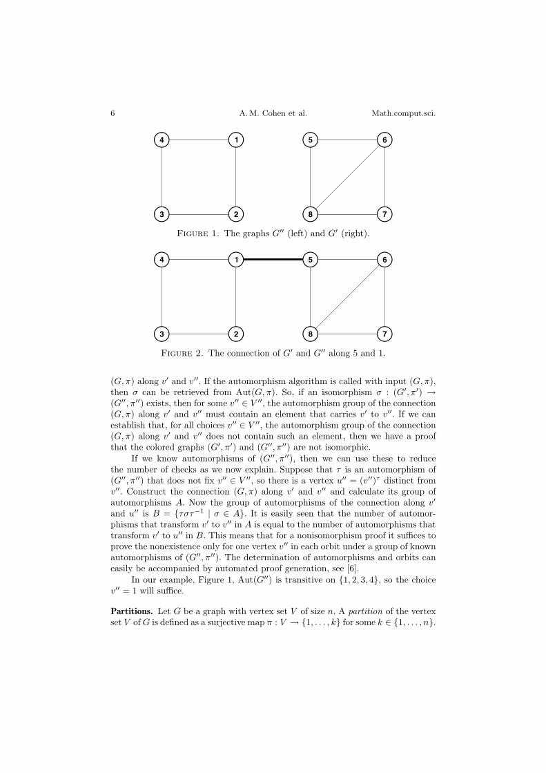
By way of example, we will take along the graphs G′ and G′′ pictured at theright and the left of Figure 1, respectively. They are clearly nonisomorphic andthis can be proven by various of the invariants listed in Section 2. We will ignorethis fact here and use them to illustrate the nauty program and our modifications.Take v′ to be the vertex labeled 5 in G′ and v′′ the vertex 1 of G′′. The connection(G, π) along 5 and 1 has vertex set {1, . . . , 8}, edges as indicated in Figure 2, andpartition π consisting of {1, 5} and {2, 3, 4, 6, 7, 8}.Graph isomorphism by means of connection. We can now determine whether thereis an isomorphism (G′, π′) → (G′′, π′′) that takes v′ to v′′, by running the auto-morphism algorithm to compute the group Aut(G, π) of automorphisms of theconnection (G, π) of (G′, π′) and (G′′, π′′) along v′ and v′′. Such automorphismsleave the edge {v′, v′′} fixed. If Aut(G, π) contains a generator that exchanges v′

and v′′, then the restriction to V ′ of that element is an isomorphism from (G′, π′)to (G′′, π′′).

Fix a vertex v′ ∈ V ′. Suppose that σ is an isomorphism from (G′, π′) to(G′′, π′′). Let v′′ ∈ V ′′ be the image of v′ under σ. We will use right actions andexponentiation to denote the image, so v′′ = (v′)σ. Now construct the connection


1

23

4 5 6

78

Figure 1. The graphs G′′ (left) and G′ (right).

1

23

4 5 6

78

Figure 2. The connection of G′ and G′′ along 5 and 1.

(G, π) along v′ and v′′. If the automorphism algorithm is called with input (G, π),then σ can be retrieved from Aut(G, π). So, if an isomorphism σ : (G′, π′) →(G′′, π′′) exists, then for some v′′ ∈ V ′′, the automorphism group of the connection(G, π) along v′ and v′′ must contain an element that carries v′ to v′′. If we canestablish that, for all choices v′′ ∈ V ′′, the automorphism group of the connection(G, π) along v′ and v′′ does not contain such an element, then we have a proofthat the colored graphs (G′, π′) and (G′′, π′′) are not isomorphic.

If we know automorphisms of (G′′, π′′), then we can use these to reducethe number of checks as we now explain. Suppose that τ is an automorphism of(G′′, π′′) that does not fix v′′ ∈ V ′′, so there is a vertex u′′ = (v′′)τ distinct fromv′′. Construct the connection (G, π) along v′ and v′′ and calculate its group ofautomorphisms A. Now the group of automorphisms of the connection along v′

and u′′ is B = {τστ−1 | σ ∈ A}. It is easily seen that the number of automor-phisms that transform v′ to v′′ in A is equal to the number of automorphisms thattransform v′ to u′′ in B. This means that for a nonisomorphism proof it suffices toprove the nonexistence only for one vertex v′′ in each orbit under a group of knownautomorphisms of (G′′, π′′). The determination of automorphisms and orbits caneasily be accompanied by automated proof generation, see [6].

In our example, Figure 1, Aut(G′′) is transitive on {1, 2, 3, 4}, so the choicev′′ = 1 will suffice.

Partitions. Let G be a graph with vertex set V of size n. A partition of the vertexset V of G is defined as a surjective map π : V → {1, . . . , k} for some k ∈ {1, . . . , n}.


A set consisting of all vertices with the same color, that is, the same π value, iscalled a cell . Here the natural ordering on N is significant for interpreting π asan ordered partition. So, the cells are ordered according to their value under π.In order to describe a partition, we will use the notation of a list, in which thecells are separated by | . For example, if V = {1, . . . , 4}, then by π = [1 | 2 4 | 3], wemean the partition π : V → {1, 2, 3} given by 1π = 1, 2π = 4π = 2, and 3π = 3. Forexample, the partition π of the connection of Figure 2 is denoted [1 5 | 2 3 4 6 7 8].

A partition is called discrete if all vertices have a different color; for example[1 | 4 | 2 | 3] is discrete. Let π and π′ be partitions of a set of vertices V . Then π iscalled finer than π′ if every cell of π is a subset of a cell of π′ and vπ′

> v′π′⇒ vπ >

v′π. Note that π is finer than itself. If π is finer than π′ and π �= π′ then π is calledstrictly finer than π′. For example, [1 | 4 | 2 | 3] is strictly finer than π = [1 | 2 4 | 3].

We will use the obvious but convenient fact that, once V is identified with{1, . . . , n}, a discrete partition of V is a permutation of {1, . . . , n}. For example,the partition [1 | 4 | 2 | 3] is nothing but the permutation (2, 4, 3), when written incycle notation.

Refinement function. Let G be a graph and π = [V1| . . . |Vk] a partition of itsvertex set V , so Vi is the inverse image under π of i for each i ∈ {1, . . . , k}. Fora sequence α of distinct cells of π, let R(G, π, α) be a partition of V , with thefollowing two properties.

1. R(G, π, α) is finer than π.2. R(Gσ, πσ, ασ) = R(G, π, α)σ, for all σ ∈ Sym(V ).

A function R with these properties is called a refinement function. Observe that,if σ is an automorphism of the colored graph (G, π), it leaves invariant all cells of πand hence α, so, by (2), R(G, π, α)σ = R(G, π, α), and σ is also an automorphismof (G,R(G, π, α)). As discrete partitions are closer to candidate automorphismsof the colored graph (in a sense to be made concrete in the context of search treesbelow), the intent is to refine π as much as possible.

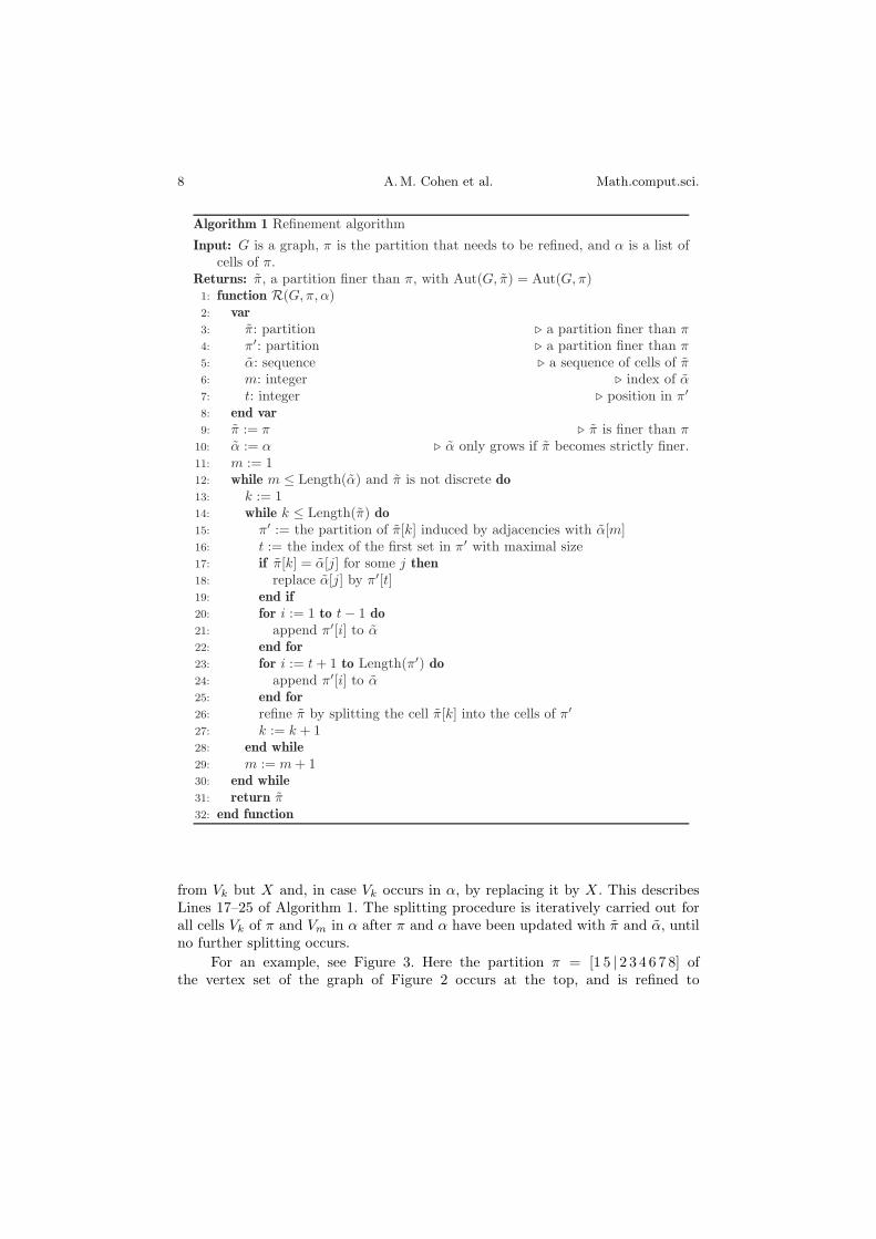
Refinement algorithm. In Algorithm 1, we give an example of a refinement func-tion that is part of nauty; cf. Algorithm 1 from [15] and Algorithm 2.5 in [16]. Thisfunction works well in the generic case. For certain special classes of graphs likethose with high symmetry, other refinement functions might give better results,cf. [2, 14, 24]. The idea behind the algorithm is to look at the number of edgesbetween cells of a partition. Let Vk be a cell of the partition π and let Vm be acell occurring in α. On Line 15 of Algorithm 1, Vk appears as π[k] and α[m] isVm′ where m′ is defined by the property that π[m′] = α[m]. For each v ∈ Vk, wecalculate the number of vertices in Vm that are adjacent to v in G. If this value isnot the same for all vertices in Vk, then we can refine π to a partition π, in whichVk is split according to the different values. Let X be the first (that is, with thesmallest π value) cell of π among the largest cells of π contained in Vk. On Line18 of Algorithm 1, X appears as π′[t]. The splitting is then also used to transformα to a sequence α in which the refinement is captured by adding all cells arising


Algorithm 1 Refinement algorithm

Input: G is a graph, π is the partition that needs to be refined, and α is a list ofcells of π.

Returns: π, a partition finer than π, with Aut(G, π) = Aut(G, π)1: function R(G, π, α)2: var3: π: partition � a partition finer than π4: π′: partition � a partition finer than π5: α: sequence � a sequence of cells of π6: m: integer � index of α7: t: integer � position in π′

8: end var9: π := π � π is finer than π

10: α := α � α only grows if π becomes strictly finer.11: m := 112: while m ≤ Length(α) and π is not discrete do13: k := 114: while k ≤ Length(π) do15: π′ := the partition of π[k] induced by adjacencies with α[m]16: t := the index of the first set in π′ with maximal size17: if π[k] = α[j] for some j then18: replace α[j] by π′[t]19: end if20: for i := 1 to t − 1 do21: append π′[i] to α22: end for23: for i := t + 1 to Length(π′) do24: append π′[i] to α25: end for26: refine π by splitting the cell π[k] into the cells of π′

27: k := k + 128: end while29: m := m + 130: end while31: return π32: end function

from Vk but X and, in case Vk occurs in α, by replacing it by X. This describesLines 17–25 of Algorithm 1. The splitting procedure is iteratively carried out forall cells Vk of π and Vm in α after π and α have been updated with π and α, untilno further splitting occurs.

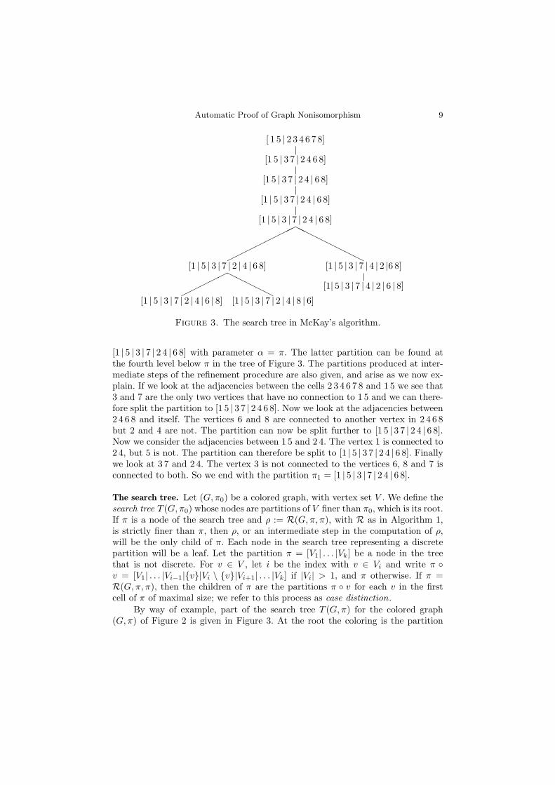
For an example, see Figure 3. Here the partition π = [1 5 | 2 3 4 6 7 8] ofthe vertex set of the graph of Figure 2 occurs at the top, and is refined to


[ 1 5 | 2 3 4 6 7 8]

[1 5 | 3 7 | 2 4 6 8]

[1 5 | 3 7 | 2 4 | 6 8]

[1 | 5 | 3 7 | 2 4 | 6 8]

[1 | 5 | 3 | 7 | 2 4 | 6 8]

��

��

[1 | 5 | 3 | 7 | 2 | 4 | 6 8]

��

��

[1 | 5 | 3 | 7 | 2 | 4 | 6 | 8] [1 | 5 | 3 | 7 | 2 | 4 | 8 | 6]

[1 | 5 | 3 | 7 | 4 | 2 |6 8]

[1| 5 | 3 | 7 | 4 | 2 | 6 | 8]

Figure 3. The search tree in McKay’s algorithm.

[1 | 5 | 3 | 7 | 2 4 | 6 8] with parameter α = π. The latter partition can be found atthe fourth level below π in the tree of Figure 3. The partitions produced at inter-mediate steps of the refinement procedure are also given, and arise as we now ex-plain. If we look at the adjacencies between the cells 2 3 4 6 7 8 and 1 5 we see that3 and 7 are the only two vertices that have no connection to 1 5 and we can there-fore split the partition to [1 5 | 3 7 | 2 4 6 8]. Now we look at the adjacencies between2 4 6 8 and itself. The vertices 6 and 8 are connected to another vertex in 2 4 6 8but 2 and 4 are not. The partition can now be split further to [1 5 | 3 7 | 2 4 | 6 8].Now we consider the adjacencies between 1 5 and 2 4. The vertex 1 is connected to2 4, but 5 is not. The partition can therefore be split to [1 | 5 | 3 7 | 2 4 | 6 8]. Finallywe look at 3 7 and 2 4. The vertex 3 is not connected to the vertices 6, 8 and 7 isconnected to both. So we end with the partition π1 = [1 | 5 | 3 | 7 | 2 4 | 6 8].

The search tree. Let (G, π0) be a colored graph, with vertex set V . We define thesearch tree T (G, π0) whose nodes are partitions of V finer than π0, which is its root.If π is a node of the search tree and ρ := R(G, π, π), with R as in Algorithm 1,is strictly finer than π, then ρ, or an intermediate step in the computation of ρ,will be the only child of π. Each node in the search tree representing a discretepartition will be a leaf. Let the partition π = [V1| . . . |Vk] be a node in the treethat is not discrete. For v ∈ V , let i be the index with v ∈ Vi and write π ◦v = [V1| . . . |Vi−1|{v}|Vi \ {v}|Vi+1| . . . |Vk] if |Vi| > 1, and π otherwise. If π =R(G, π, π), then the children of π are the partitions π ◦ v for each v in the firstcell of π of maximal size; we refer to this process as case distinction.

By way of example, part of the search tree T (G, π) for the colored graph(G, π) of Figure 2 is given in Figure 3. At the root the coloring is the partition


π0 = π with color 1 for {1, 5} and color 2 for {3, 4, 6, 7, 8}. The tree does notbranch out before π1 = [1 | 5 | 3 | 7 | 2 4 | 6 8]. As mentioned earlier, the partitionsabove π1 are intermediate steps of the computation π1 = R(G, π, π).

The search tree T (G, π0) can be used to compute the automorphism groupof a colored graph (G, π0) as follows. Fix a discrete partition p of V occurring asa leaf in the search tree. A second leaf p′ of the search tree then determines thebijection p−1p′ of V , which preserves the least common partition of p and p′ inT (G, π0). By checking whether this bijection is an automorphism of (G, π0) foreach leaf p′, the automorphism group can be determined elementwise.

Clearly, checking all discrete partitions is not efficient. The refinement builtinto the search tree is already of help in that it restricts the search to those per-mutations that respect given refinements of the partition induced by the initialcoloring π0. Furthermore it suffices to construct a set of generators of the auto-morphism group rather than all of its elements. The generating automorphismsalready found can be used to reduce the number of children in the search tree thatneed to be perused. For, the choices of the vertex v in the case distinction above canbe restricted to representatives of the orbits of the group of automorphisms foundwithin the cell that is being split. Algorithm 2 exhibits the code involved. The listof generators found is stored in R and the subgroup of Aut(G, π0) generated by Ris denoted 〈R〉.

In general, it is not necessary to carry out the full refinement procedure. Itsuffices to restrict to steps in which the partitions are made finer in parallel waysas follows: if ρ = [U1| · · · |Uk] and σ = [V1| · · · |Vk] are two nodes on the same levelof the search tree and there are Ui and Uj such that the number of vertices in Uj

adjacent to v is not the same for each v ∈ Ui, then also the number of vertices inVj adjacent to v is not the same for each v ∈ Vi. For, if p refines ρ and p′ refinesσ, then, for p−1p′ to be an automorphism of (G, π), it must map ρ to σ.

For our example graphs of Figure 1, consider once more the search tree asgiven in Figure 3. Further nodes are formed by refinement and case distinction.Since the partition π1 = [1 | 5 | 3 | 7 | 2 4 | 6 8] cannot be split further by refinement(it is not necessary to prove this), the children of the corresponding node arefound by case distinction of 2 4: we can color 2 4 by a partition π refining thenode so that 2π < 4π or so that 4π < 2π. In the left branch we have a casedistinction again for the cell 6 8 and we find the first two leaves. The first leaf is[1 | 5 | 3 | 7 | 2 | 4 | 6 | 8] which is our reference partition p, and so gives the identitymap on the vertex set of G. The second leaf is p′ = [1 | 5 | 3 | 7 | 2 | 4 | 8 | 6], that is,the permutation (2, 5)(4, 7, 8, 6), and leads to the automorphism p−1p′ = (6, 8).Now we return to the case 4π < 2π. Since we know that 6 and 8 are in the sameorbit under permutations that stabilize 2 and 4, we may assume 6π < 8π. This givesus another leaf p′ = [1 | 5 | 3 | 7 | 4 | 2 | 6 | 8], in cycle notation (2, 5, 4, 7, 6), resultingin the automorphism p−1p′ = (2, 5)(4, 6, 7)(2, 5, 4, 7, 6) = (2, 4). The leaves of thesearch tree are now exhausted, so the automorphism group of G is 〈(2, 4), (6, 8)〉.There are no automorphisms that interchange 1 and 5, and therefore the graphsG′ and G′′ are not isomorphic.


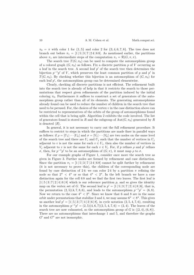
Algorithm 2 Finding generating automorphisms

Input: (G, π) is a colored graph, p is a discrete partition finer than π, and α is alist of cells from π used to refine π.

Returns: R is a set of generators of Aut(G, π).1: function FindAutomorphisms(G, p, π, α)2: var3: c: cell � c is the first cell of π of maximal length4: v: vertex � v ∈ c5: ρ: partition � ρ is finer than π6: M : set of vertices � used to mark vertices in c7: end var8: R := ∅9: M := ∅

10: ρ := R(G, π, α)11: if ρ is discrete then � ρ defines a permutation12: if p−1ρ ∈ Aut(G, π) then � p′ = ρ13: R := {p−1ρ}14: end if15: else � recursion16: c := the first cell of ρ of maximal length17: for v ∈ c do18: if vσ ∈ M for some σ in 〈R〉 with ρσ = ρ then19: do nothing � no new generator will be found20: else21: R := R ∪ FindAutomorphisms(G, p, ρ ◦ v, [{v}])22: M := M ∪ {v}23: end if24: end for25: end if26: return R27: end function

4. A proof constructor

In this section, we report on a software package that automatically constructs aproof of (non)isomorphism of two given graphs.

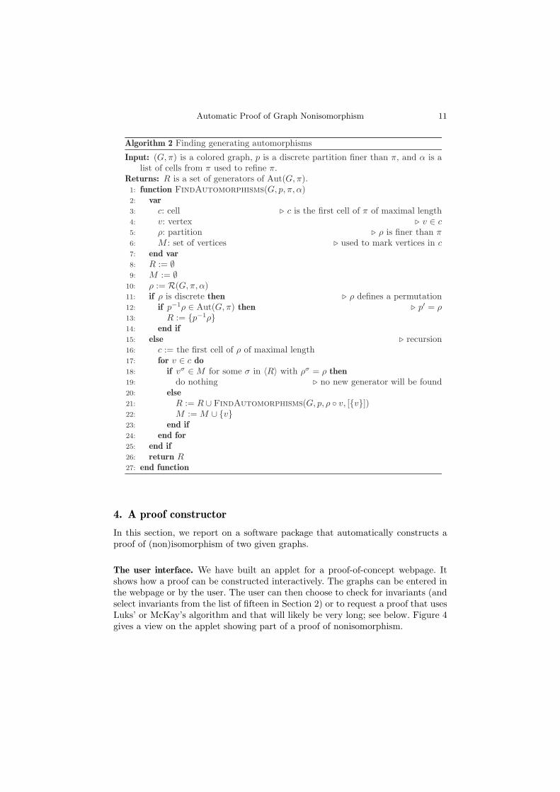
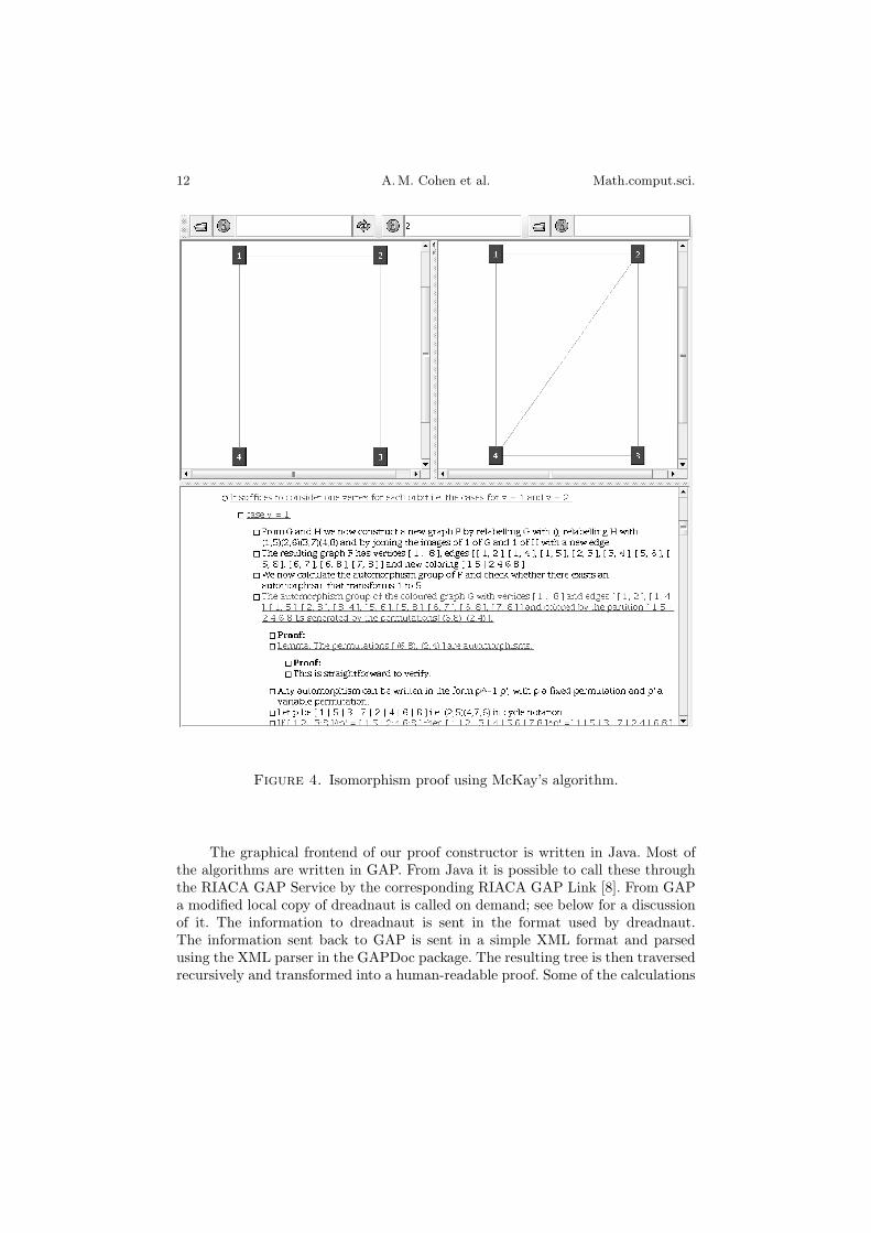
The user interface. We have built an applet for a proof-of-concept webpage. Itshows how a proof can be constructed interactively. The graphs can be entered inthe webpage or by the user. The user can then choose to check for invariants (andselect invariants from the list of fifteen in Section 2) or to request a proof that usesLuks’ or McKay’s algorithm and that will likely be very long; see below. Figure 4gives a view on the applet showing part of a proof of nonisomorphism.


Figure 4. Isomorphism proof using McKay’s algorithm.

The graphical frontend of our proof constructor is written in Java. Most ofthe algorithms are written in GAP. From Java it is possible to call these throughthe RIACA GAP Service by the corresponding RIACA GAP Link [8]. From GAPa modified local copy of dreadnaut is called on demand; see below for a discussionof it. The information to dreadnaut is sent in the format used by dreadnaut.The information sent back to GAP is sent in a simple XML format and parsedusing the XML parser in the GAPDoc package. The resulting tree is then traversedrecursively and transformed into a human-readable proof. Some of the calculations


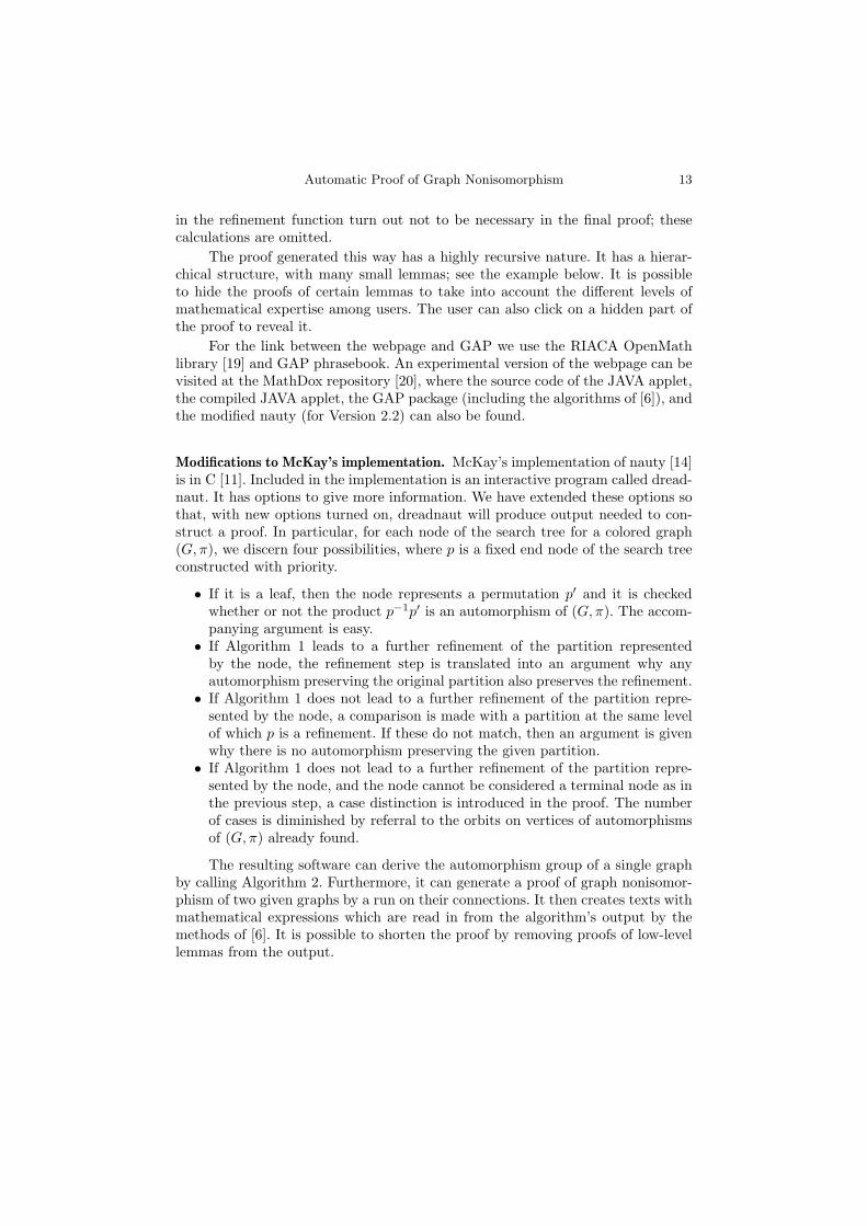
in the refinement function turn out not to be necessary in the final proof; thesecalculations are omitted.

The proof generated this way has a highly recursive nature. It has a hierar-chical structure, with many small lemmas; see the example below. It is possibleto hide the proofs of certain lemmas to take into account the different levels ofmathematical expertise among users. The user can also click on a hidden part ofthe proof to reveal it.

For the link between the webpage and GAP we use the RIACA OpenMathlibrary [19] and GAP phrasebook. An experimental version of the webpage can bevisited at the MathDox repository [20], where the source code of the JAVA applet,the compiled JAVA applet, the GAP package (including the algorithms of [6]), andthe modified nauty (for Version 2.2) can also be found.

Modifications to McKay’s implementation. McKay’s implementation of nauty [14]is in C [11]. Included in the implementation is an interactive program called dread-naut. It has options to give more information. We have extended these options sothat, with new options turned on, dreadnaut will produce output needed to con-struct a proof. In particular, for each node of the search tree for a colored graph(G, π), we discern four possibilities, where p is a fixed end node of the search treeconstructed with priority.

• If it is a leaf, then the node represents a permutation p′ and it is checkedwhether or not the product p−1p′ is an automorphism of (G, π). The accom-panying argument is easy.

• If Algorithm 1 leads to a further refinement of the partition representedby the node, the refinement step is translated into an argument why anyautomorphism preserving the original partition also preserves the refinement.

• If Algorithm 1 does not lead to a further refinement of the partition repre-sented by the node, a comparison is made with a partition at the same levelof which p is a refinement. If these do not match, then an argument is givenwhy there is no automorphism preserving the given partition.

• If Algorithm 1 does not lead to a further refinement of the partition repre-sented by the node, and the node cannot be considered a terminal node as inthe previous step, a case distinction is introduced in the proof. The numberof cases is diminished by referral to the orbits on vertices of automorphismsof (G, π) already found.

The resulting software can derive the automorphism group of a single graphby calling Algorithm 2. Furthermore, it can generate a proof of graph nonisomor-phism of two given graphs by a run on their connections. It then creates texts withmathematical expressions which are read in from the algorithm’s output by themethods of [6]. It is possible to shorten the proof by removing proofs of low-levellemmas from the output.


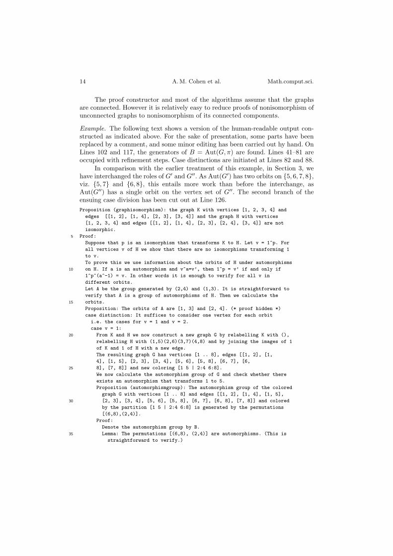
The proof constructor and most of the algorithms assume that the graphsare connected. However it is relatively easy to reduce proofs of nonisomorphism ofunconnected graphs to nonisomorphism of its connected components.

Example. The following text shows a version of the human-readable output con-structed as indicated above. For the sake of presentation, some parts have beenreplaced by a comment, and some minor editing has been carried out hy hand. OnLines 102 and 117, the generators of B = Aut(G, π) are found. Lines 41–81 areoccupied with refinement steps. Case distinctions are initiated at Lines 82 and 88.

In comparison with the earlier treatment of this example, in Section 3, wehave interchanged the roles of G′ and G′′. As Aut(G′) has two orbits on {5, 6, 7, 8},viz. {5, 7} and {6, 8}, this entails more work than before the interchange, asAut(G′′) has a single orbit on the vertex set of G′′. The second branch of theensuing case division has been cut out at Line 126.Proposition (graphisomorphism): the graph K with vertices [1, 2, 3, 4] and

edges [[1, 2], [1, 4], [2, 3], [3, 4]] and the graph H with vertices

[1, 2, 3, 4] and edges [[1, 2], [1, 4], [2, 3], [2, 4], [3, 4]] are not

isomorphic.

Proof:5

Suppose that p is an isomorphism that transforms K to H. Let v = 1^p. For

all vertices v of H we show that there are no isomorphisms transforming 1

to v.

To prove this we use information about the orbits of H under automorphisms

on H. If a is an automorphism and v^a=v’, then 1^p = v’ if and only if10

1^p^(a^-1) = v. In other words it is enough to verify for all v in

different orbits.

Let A be the group generated by (2,4) and (1,3). It is straightforward to

verify that A is a group of automorphisms of H. Then we calculate the

orbits.15

Proposition: The orbits of A are [1, 3] and [2, 4]. (* proof hidden *)

case distinction: It suffices to consider one vertex for each orbit

i.e. the cases for v = 1 and v = 2.

case v = 1:

From K and H we now construct a new graph G by relabelling K with (),20

relabelling H with (1,5)(2,6)(3,7)(4,8) and by joining the images of 1

of K and 1 of H with a new edge.

The resulting graph G has vertices [1 .. 8], edges [[1, 2], [1,

4], [1, 5], [2, 3], [3, 4], [5, 6], [5, 8], [6, 7], [6,

8], [7, 8]] and new coloring [1 5 | 2:4 6:8].25

We now calculate the automorphism group of G and check whether there

exists an automorphism that transforms 1 to 5.

Proposition (automorphismgroup): The automorphism group of the colored

graph G with vertices [1 .. 8] and edges [[1, 2], [1, 4], [1, 5],

[2, 3], [3, 4], [5, 6], [5, 8], [6, 7], [6, 8], [7, 8]] and colored30

by the partition [1 5 | 2:4 6:8] is generated by the permutations

[(6,8),(2,4)].

Proof:

Denote the automorphism group by B.

Lemma: The permutations [(6,8), (2,4)] are automorphisms. (This is35

straightforward to verify.)


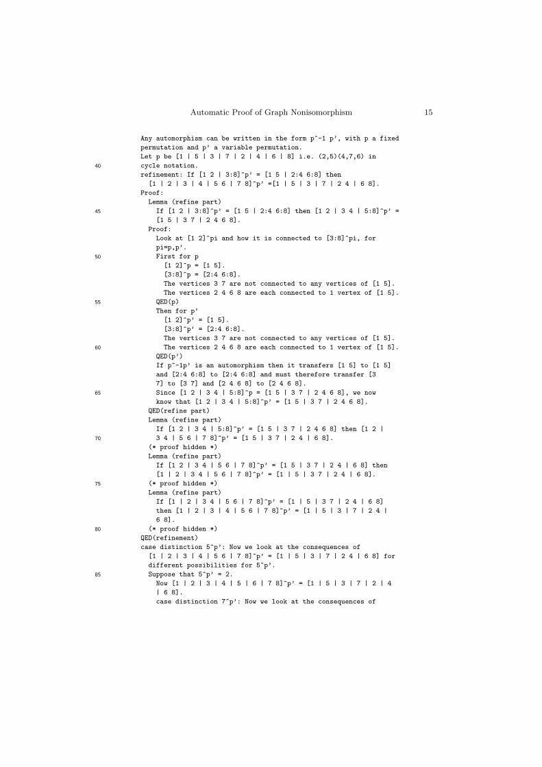
Any automorphism can be written in the form p^-1 p’, with p a fixed

permutation and p’ a variable permutation.

Let p be [1 | 5 | 3 | 7 | 2 | 4 | 6 | 8] i.e. (2,5)(4,7,6) in

cycle notation.40

refinement: If [1 2 | 3:8]^p’ = [1 5 | 2:4 6:8] then

[1 | 2 | 3 | 4 | 5 6 | 7 8]^p’ =[1 | 5 | 3 | 7 | 2 4 | 6 8].

Proof:

Lemma (refine part)

If [1 2 | 3:8]^p’ = [1 5 | 2:4 6:8] then [1 2 | 3 4 | 5:8]^p’ =45

[1 5 | 3 7 | 2 4 6 8].

Proof:

Look at [1 2]^pi and how it is connected to [3:8]^pi, for

pi=p,p’.

First for p50

[1 2]^p = [1 5].

[3:8]^p = [2:4 6:8].

The vertices 3 7 are not connected to any vertices of [1 5].

The vertices 2 4 6 8 are each connected to 1 vertex of [1 5].

QED(p)55

Then for p’

[1 2]^p’ = [1 5].

[3:8]^p’ = [2:4 6:8].

The vertices 3 7 are not connected to any vertices of [1 5].

The vertices 2 4 6 8 are each connected to 1 vertex of [1 5].60

QED(p’)

If p^-1p’ is an automorphism then it transfers [1 5] to [1 5]

and [2:4 6:8] to [2:4 6:8] and must therefore transfer [3

7] to [3 7] and [2 4 6 8] to [2 4 6 8].

Since [1 2 | 3 4 | 5:8]^p = [1 5 | 3 7 | 2 4 6 8], we now65

know that [1 2 | 3 4 | 5:8]^p’ = [1 5 | 3 7 | 2 4 6 8].

QED(refine part)

Lemma (refine part)

If [1 2 | 3 4 | 5:8]^p’ = [1 5 | 3 7 | 2 4 6 8] then [1 2 |

3 4 | 5 6 | 7 8]^p’ = [1 5 | 3 7 | 2 4 | 6 8].70

(* proof hidden *)

Lemma (refine part)

If [1 2 | 3 4 | 5 6 | 7 8]^p’ = [1 5 | 3 7 | 2 4 | 6 8] then

[1 | 2 | 3 4 | 5 6 | 7 8]^p’ = [1 | 5 | 3 7 | 2 4 | 6 8].

(* proof hidden *)75

Lemma (refine part)

If [1 | 2 | 3 4 | 5 6 | 7 8]^p’ = [1 | 5 | 3 7 | 2 4 | 6 8]

then [1 | 2 | 3 | 4 | 5 6 | 7 8]^p’ = [1 | 5 | 3 | 7 | 2 4 |

6 8].

(* proof hidden *)80

QED(refinement)

case distinction 5^p’: Now we look at the consequences of

[1 | 2 | 3 | 4 | 5 6 | 7 8]^p’ = [1 | 5 | 3 | 7 | 2 4 | 6 8] for

different possibilities for 5^p’.

Suppose that 5^p’ = 2.85

Now [1 | 2 | 3 | 4 | 5 | 6 | 7 8]^p’ = [1 | 5 | 3 | 7 | 2 | 4

| 6 8].

case distinction 7^p’: Now we look at the consequences of


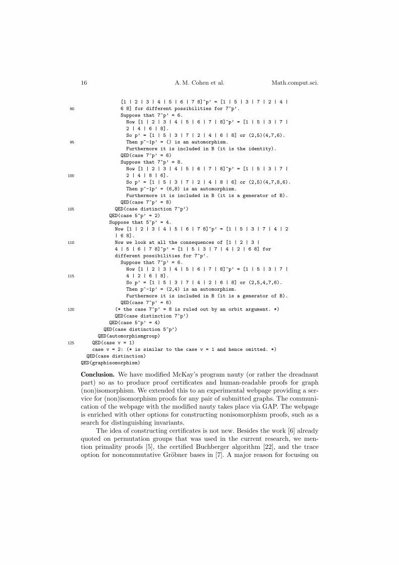
[1 | 2 | 3 | 4 | 5 | 6 | 7 8]^p’ = [1 | 5 | 3 | 7 | 2 | 4 |

6 8] for different possibilities for 7^p’.90

Suppose that 7^p’ = 6.

Now [1 | 2 | 3 | 4 | 5 | 6 | 7 | 8]^p’ = [1 | 5 | 3 | 7 |

2 | 4 | 6 | 8].

So p’ = [1 | 5 | 3 | 7 | 2 | 4 | 6 | 8] or (2,5)(4,7,6).

Then p^-1p’ = () is an automorphism.95

Furthermore it is included in B (it is the identity).

QED(case 7^p’ = 6)


Now [1 | 2 | 3 | 4 | 5 | 6 | 7 | 8]^p’ = [1 | 5 | 3 | 7 |

2 | 4 | 8 | 6].100

So p’ = [1 | 5 | 3 | 7 | 2 | 4 | 8 | 6] or (2,5)(4,7,8,6).

Then p^-1p’ = (6,8) is an automorphism.

Furthermore it is included in B (it is a generator of B).


QED(case distinction 7^p’)105



Now [1 | 2 | 3 | 4 | 5 | 6 | 7 8]^p’ = [1 | 5 | 3 | 7 | 4 | 2

| 6 8].

Now we look at all the consequences of [1 | 2 | 3 |110

4 | 5 | 6 | 7 8]^p’ = [1 | 5 | 3 | 7 | 4 | 2 | 6 8] for

different possibilities for 7^p’.


Now [1 | 2 | 3 | 4 | 5 | 6 | 7 | 8]^p’ = [1 | 5 | 3 | 7 |

4 | 2 | 6 | 8].115

So p’ = [1 | 5 | 3 | 7 | 4 | 2 | 6 | 8] or (2,5,4,7,6).

Then p^-1p’ = (2,4) is an automorphism.

Furthermore it is included in B (it is a generator of B).


(* the case 7^p’ = 8 is ruled out by an orbit argument. *)120

QED(case distinction 7^p’)


QED(case distinction 5^p’)

QED(automorphismgroup)

QED(case v = 1)125

case v = 2: (* is similar to the case v = 1 and hence omitted. *)

QED(case distinction)

QED(graphisomorphism)

Conclusion. We have modified McKay’s program nauty (or rather the dreadnautpart) so as to produce proof certificates and human-readable proofs for graph(non)isomorphism. We extended this to an experimental webpage providing a ser-vice for (non)isomorphism proofs for any pair of submitted graphs. The communi-cation of the webpage with the modified nauty takes place via GAP. The webpageis enriched with other options for constructing nonisomorphism proofs, such as asearch for distinguishing invariants.

The idea of constructing certificates is not new. Besides the work [6] alreadyquoted on permutation groups that was used in the current research, we men-tion primality proofs [5], the certified Buchberger algorithm [22], and the traceoption for noncommutative Grobner bases in [7]. A major reason for focusing on


graph nonisomorphism is its significance for a wide range of applications, varyingfrom image analysis [4] and organic molecule structures [23] to designs of experi-ments [18].

Because of the exponential growth in the lengths of the proofs produced, ourmodified version of McKay’s algorithm is only practical for relatively small graphs.Invariants can frequently distinguish much larger graphs, however.

We benchmarked our invariants with the series of all 3854 nonisomorphicstrongly-regular graphs with parameters (35, 16, 6, 8) available on McKay’s web-page [17]. By definition, in such a graph there are exactly 35 vertices, each vertexhas degree 16, on each edge there are precisely 6 triangles, and each pair of non-adjacent vertices has exactly 8 common neighbors. Because of their regularity, themost straightforward invariants will not separate them. Of the first fourteen in-variants, (13), the multiset of numbers of K2,1,1-graphs per edge, turned out to bethe most effective distinguisher. It takes 3487 values on the graphs, whereas forinstance invariant (10) only takes 5 different values. Invariant (15), the multiset ofall local K2,1,1-graph numbers, has 3804 different values. Using (16), the multisetof all local adjacency matrix powers, in addition to (15), we can distinguish themall.

The package is experimental and bigger graphs still lead to huge output. Fine-tuning by skipping subroutines from [6] will lead to a considerable improvement ofthe performance. Also the protocol and the implementation of the communicationbetween processes leaves room for speed up. At the moment a lot of information issent from dreadnaut to GAP. A more efficient coupling will also diminish runningtimes.

A more mathematical approach to shortening the proofs would be to usean initial coloring of the graph. For instance, the user could introduce a vertexinvariant as the coloring in the first step of McKay’s algorithm. In the example ofSection 4, the case v = 2 could be ruled out by the observation that the valenceof vertex 6 in G does not match the valence of vertex 2 in G.

Adding these options to the webpage would lead to a better proof assistantin that invariants could be introduced to shorten automatically generated proofs.Also, the nauty user’s guide [14] describes further refinements already implementedin nauty but not employed by us for proof generation. Furthermore, in order tobe able to deal with more regular graphs, refinements based on edges, and morecomplicated structures than vertices, could be incorporated, as proposed in [24].

References

[1] L. Babai, Moderately exponential bound for graph isomorphism. In Fundamentals ofcomputation theory (Szeged, 1981), vol. 117 of Lecture Notes in Comput. Sci., pages34–50. Springer, Berlin, 1981.

[2] L. Babel, I. V. Chuvaeva, M. Klin, and D. V. Pasechnik, Program implementation ofthe Weisfeiler-Leman algorithm. In Algebraic Combinatorics in Mathematical Chem-istry. Methods and Algorithms, vol. TUM-M9701, pages 1–45, 1997.


[3] H. Barendregt and A. M. Cohen, Electronic communication of mathematics and theinteraction of computer algebra systems and proof assistants. J. Symb. Comput.,32(1–2):3–22, 2001.

[4] H. Bunke and B. T. Messmer, Efficient attributed graph matching and its applicationto image analysis. In ICIAP ’95: Proceedings of the 8th International Conference onImage Analysis and Processing, pages 45–55, London, UK, 1995. Springer Verlag.

[5] O. Caprotti and M. Oostdijk, Formal and efficient primality proofs by use of com-puter algebra oracles. J. Symbolic Comput., 32(1–2):55–70, 2001. Computer algebraand mechanized reasoning (St. Andrews, 2000).

[6] A. Cohen, S. Murray, M. Pollet, and V. Sorge, Certifying solutions to permutationgroup problems. In Franz Baader, editor, 19th International Conference on Auto-mated Deduction, pages 258–273. Springer Verlag, Berlin, 2003.

[7] A. M. Cohen, Documentation on the gbnp package, 2007. Available from World WideWeb: http://www.mathdox.org/products/gbnp/.

[8] RIACA GAP phrasebook, 2004. Available from World Wide Web: http://www.

mathdox.org/phrasebook/gap/.

[9] J. Harrison and L. Thery, A skeptic’s approach to combining HOL and Maple. J. Au-tom. Reasoning, 21(3):279–294, 1998.

[10] C. S. Iliopoulos, Worst-case complexity bounds on algorithms for computing thecanonical structure of finite abelian groups and the Hermite and Smith normal formsof an integer matrix. SIAM J. Comput., 18(4):658–669, 1989.

[11] B. W. Kernighan and D. M. Ritchie, The C Programming Language, Second Edition.Prentice-Hall, Englewood Cliffs, New Jersey, 1988.

[12] A. R. Klivans and D. van Melkebeek, Graph nonisomorphism has subexponential sizeproofs unless the polynomial-time hierarchy collapses. SIAM J. Comput., 31(5):1501–1526 (electronic), 2002.

[13] E. M. Luks, Isomorphism of graphs of bounded valence can be tested in polynomialtime. J. Comput. System Sci., 25(1):42–65, 1982.

[14] B. D. McKay, nauty User’s Guide. Computer Science Department Australian Na-tional University, ACT 0200, Australia. Available from World Wide Web: http:

//cs.anu.edu.au/~bdm/nauty/nug.pdf. version 2.2.

[15] B. D. McKay, Computing automorphisms and canonical labellings of graphs. In Com-binatorial mathematics (Proc. Internat. Conf. Combinatorial Theory, AustralianNat. Univ., Canberra, 1977), vol. 686 of Lecture Notes in Math., pages 223–232.Springer, Berlin, 1978.

[16] B. D. McKay, Practical graph isomorphism. In Proceedings of the Tenth ManitobaConference on Numerical Mathematics and Computing, vol. I, (Winnipeg, Man.,1980), vol. 30, pages 45–87, 1981.

[17] Lists of nonisomorphic strongly-regular graphs, 2008. Available from World WideWeb: http://cs.anu.edu.au/~bdm/data/graphs.html.

[18] N. Van Minh Man, On Construction and Identification of Graphs. Technische Uni-versiteit Eindhoven, Eindhoven, 2005. PhD Thesis.

[19] RIACA OpenMath library, 2004. Available from World Wide Web: http://www.

mathdox.org/omlib/.


[20] Proof assistant for graph non-isomorphism, 2006. Available from World Wide Web:http://www.mathdox.org/graphiso/.

[21] N. Shankar, Little engines of proof. In FME, pages 1–20, 2002.

[22] L. Thery, A certified version of Buchberger’s algorithm. In CADE-15: Proceedings ofthe 15th International Conference on Automated Deduction, pages 349–364, London,UK, 1998. Springer Verlag.

[23] M. I. Trofimov and N.D. Zelinsky, Application of the electronegativity indices of or-ganic molecules to tasks of chemical informatics. Russian Chemical Bulletin, 54:2235–2246, 2005.

[24] B. Weisfeiler, On Construction and Identification of Graphs. Springer Verlag, Berlin,1976. With contributions by A. Lehman, G. M. Adelson-Velsky, V. Arlazarov,I. Faragev, A. Uskov, I. Zuev, M. Rosenfeld and B. Weisfeiler, B. Weisfeiler (ed.),Lecture Notes in Mathematics, Vol. 558.

Arjeh M. Cohen and Jan Willem KnopperDepartment of Mathematics and Computer ScienceTechnische Universiteit EindhovenPO Box 513NL-5600 MB EindhovenThe Netherlandse-mail: [email protected]

[email protected]

Scott H. MurrayDepartment of Mathematics and StatisticsUniversity of SydneyNSW 2006Australiae-mail: [email protected]

Received: December 14, 2007.

Revised: March 14, 2008.

Accepted: June 4, 2008.

Documents

Automatic Proof of Graph Nonisomorphism · For mathematical problems, ... operations. By counting, for each vertex, ... Automatic Proof of Graph Nonisomorphism 5Published in: Mathematics