EUROPEAN ECONOMY

Economic Papers 452 | April 2012

Automatic Fiscal Stabilisers: What they are and what they do

Economic and Financial Aff airs

Jan in ‘t Veld, Martin Larch andMarieke Vandeweyer

Economic Papers are written by the Staff of the Directorate-General for Economic and Financial Aff airs, or by experts working in association with them. The Papers are intended to increase awareness of the technical work being done by staff and to seek comments and suggestions for further analysis. The views expressed are the author’s alone and do not necessarily correspond to those of the European Commis-sion. Comments and enquiries should be addressed to:

European CommissionDirectorate-General for Economic and Financial Aff airsPublicationsB-1049 BrusselsBelgiumE-mail: Ecfi n-Info@ec.europa.eu

This paper exists in English only and can be downloaded from the website ec.europa.eu/economy_fi nance/publications

A great deal of additional information is available on the Internet. It can be accessed through the Europa server (ec.europa.eu)

ISBN 978-92-79-22973-2doi: 10.2765/25943

© European Union, 2012

0

Automatic Fiscal Stabilisers:

What they are and what they do.

Jan in't Veld*

Martin Larch†

Marieke Vandeweyer‡

This draft:

27 March 2010 Abstract

The global financial and economic crisis has revived the debate in the academic literature and in policy circles about the size and effectiveness of automatic fiscal stabilisers. Especially in the euro area where monetary policy is centralised and discretionary fiscal policy making is constrained by the EU fiscal rules, knowing the size and the effectiveness of automatic stabilisers is crucial. While automatic stabilisers are a fairly established concept in the fiscal policy literature, there is still no consensus about their actual nature and their effectiveness. This paper shows that differences in opinion mirror a deeper disagreement over how the budget would look like without automatic stabilisers. This issue is addressed by defining two types of counterfactual budgets giving rise to two different interpretations about the nature of automatic stabilisation. Simulations with a structural model confirm that the degree of smoothing is conditional on how the counterfactual budget, i.e. the budget without automatic stabilisers, is defined.

Keywords: Automatic stabilisers, budget balance, output smoothing, model simulation JEL classification: H6, H30, E37, E62

__________________ We thank Lukas Vogel for useful comments on an earlier draft. The views expressed in this paper are those of the authors and should not be attributed to the European Commission.

* European Commission Directorate-General for Economic and Financial Affairs, Rue de la Loi 200, 1049 Bruxelles, email: jan.intveld@ec.europa.eu. † Corresponding author, European Commission Directorate-General for Economic and Financial Affairs, email: martin.larch@ec.europa.eu. ‡ Katholieke Universiteit Leuven – Faculty of Business and Economics, Naamsestraat 69, 3000 Leuven, email: marieke.vandeweyer@econ.kuleuven.be.

1

1. Introduction and motivation

The post-2007 economic and financial crisis has reopened the debate on the effectiveness of

fiscal policy as a tool of stabilisation of economic activity, including the relative merits of

discretionary action versus automatic stabilisation. On one side of the debate, people have

argued that discretionary fiscal policy is not an effective stabilisation tool. Especially from a

political economy point of view, long decision and implementation lags associated with

discretionary fiscal policy are often mentioned as arguments why such policies might be

ineffective. According to this view, one should instead rely on the workings of automatic

stabilisers to do their job in stabilising the economy as any attempt to stabilise via

discretionary measures is destined to be counter-productive. A comprehensive overview of

these types of arguments is provided in e.g. Hemming et al. (2002), Taylor (2009), and Cogan

et al. (2010). Others have argued the severity of the crisis required automatic stabilisers to be

complemented by discretionary action and that the persistence of the crisis meant

implementation lags were arguably of lesser importance than under normal circumstances.

This camp emphasised the presence of financially constrained households and

accommodative monetary policy when interest rates are constrained by the zero lower bound,

two factors that render discretionary fiscal policy effective again and raise the size of the

fiscal multiplier (see e.g. Christiano, Eichenbaum and Rebelo, 2011, Davig and Leeper (2011)

and Coenen et al., 2012). Both sides of this debate would agree that the main advantage of

automatic fiscal stabilisers is that they do no not require deliberate intervention by

government and hence are not subject to implementation lags. But the crucial questions is

how much output stabilisation they deliver.

In spite of a relatively large and seasoned body of literature on automatic stabilisers, both the

policy and the academic debate reveal a persisting lack of clarity about what automatic fiscal

stabilisers actually are and how to assess their effectiveness with respect to output smoothing.

Except for the notional understanding that automatic stabilisers involve budgetary

arrangements that help smooth output without the explicit intervention of a country's fiscal

authority, views still very much diverge about which elements or components of the budget

actually provide the bulk of automatic stabilisation over the cycle. There are no doubts

concerning unemployment benefits: they unambiguously increase during downturns and

decrease in upswings. However, from a practical point of view, unemployment benefits are

rather negligible as they account for a very small share of governments' budget in most

2

advanced countries. The bulk of automatic stabilisation originates somewhere else; but

where?

The aim of this paper is to clarify the nature, size and effect of these automatic stabilisers.

Special attention is given to the relevance of defining the correct benchmark against which the

effectiveness of automatic stabilisers is measured. By making the counterfactual explicit, it

also becomes evident that diverging views and estimates in the literature are the reflection of

different, and most of time implicit, assumptions about a 'cyclically-neutral' budget. 1

The analysis of fiscal stabilisation is especially relevant in the EU, in view of the specifics of

the EU macroeconomic policy framework. In the Economic and Monetary Union (EMU)

monetary policy making is centralised and delegated to the European Central Bank (ECB).

Hence, individual member states are left with fiscal policy to stabilize their economies in the

event of idiosyncratic shocks. At the same time, fiscal policy is to be carried out within the

boundaries of the Stability and Growth Pact (SGP) which, in a nutshell, requires member

states to avoid excessive deficits and to achieve a medium term objective which ensures the

long-term stability of public finances. The new fiscal compact goes even further and sets a

legally binding maximum structural deficit of 0.5% of GDP while the maximum actual deficit

cannot exceed 3% of GDP. This leaves no room for discretionary fiscal policy and highlights

the importance of knowing whether automatic stabilisers alone can deliver sufficient

stabilisation.

The remainder of the paper is organised as follows. Section 2 takes a look at the existing

literature and highlights the different interpretations of the concept of automatic stabilisers.

Section 3 examines the background to the different interpretations by clarifying the role of the

benchmark budget against which the effect of automatic stabilisers is to be assessed. Section 4

provides an overview of empirical estimates of the effect of automatic stabilisers in the

literature. This is followed by simulations mimicking the shocks experienced during the post-

2007 recession with a calibrated structural model for the euro area. The effectiveness of

automatic stabilisation in terms of smoothing output is then assessed by a comparison with

alternative scenarios in which expenditure and revenue are kept constant in levels or as share

of GDP. The simulation results underscore the fact that the degree of output smoothing of 1 Our analysis is purely positive and we are not concerned with normative implications of automatic stabilisers. Some of the macroeconomic literature would suggest that sizeable macroeconomic fluctuations may be desirable adjustment to shocks from a welfare perspective and a normative analysis should consider the potential of automatic stabilisers to remove or mitigate welfare losses associated with nominal and real rigidities in the economy.

3

automatic stabilisers crucially depends on the counterfactual budget, that is, the budget

without automatic stabilisers.

2. Automatic stabilisers: An old friend with a fuzzy profile?

Automatic stabilisers are an integral part of the fiscal policy arsenal of a country. On the

revenue side, taxes are a very obvious and much discussed source of automatic stabilisation

(see for instance Auerbach and Feenberg, 2000). Over the cycle, tax revenues tend to follow

their respective tax base: they increase during upturns and shrink during downturns. On the

expenditure side, the most prominent automatic stabiliser discussed in the literature are

unemployment benefits. Their total amount increases during downturns and decreases during

upswings. Melitz and Darby (2008) argue that age- and health related social expenditure also

reacts to the cycle in a stabilizing manner. Hajdenberg et al. (2010), by contrast, conclude

that in developed countries social spending is a-cyclical.

However, automatic stabilisation is not necessarily limited to cyclically sensitive items in the

budget. In the literature, the size of the government is also associated with automatic

stabilisation. Research has shown that the size of government is negatively correlated with the

volatility of GDP (e.g. Fatás and Mihov, 2001; Lee and Sung, 2007). This can be explained by

the fact that the bulk of government discretionary expenditure, such as wages and transfers, is

generally not cut during economic downturns or increased during upturns. This inertia of

government expenditure has a stabilising effect on total output. Rodrik (1998) for instance

argues that open economies tend to have bigger governments so as to protect themselves from

their larger exposure to external shocks.

Overall, while we all have an intuitive understanding of what they are, there is no agreed view

in the literature on the relative importance of the different elements of automatic stabilisers.

Some claim that stabilisation mainly results from the cyclical sensitivity of revenues; others

associate the bulk of automatic stabilisers with the size and inertia of discretionary spending,

while still others believe that progressive taxation and unemployment benefits are the sole

source of automatic stabilisation.

When analysing automatic stabilisers, one can look at both their size and their degree of

output smoothing. The size of the automatic stabilisers is generally defined as the change in

4

the budget resulting from a change in economic activity. In general, there are two types of

indicators to measure this change: the budgetary sensitivity and the semi-elasticity.

The budgetary sensitivity, which for instance is used by the European Commission in the

context of the EU fiscal surveillance framework, measures the change in the level of revenues

and expenditure resulting from a marginal change in GDP:

dYdR

YR

RY

dYdR

YR

RR =úû

ùêë

é÷øö

çèæ== qe

dYdG

YG

GY

dYdG

YG

GG =úû

ùêë

é÷øö

çèæ== qe

Where R denotes government revenues, G government expenditure, and Rq and Rq the GDP

elasticity of government revenues and expenditure respectively.

The budgetary semi-elasticity, which is used by the IMF and the OECD, measures the

reaction of the ratios of expenditure and revenues to GDP to a relative change in GDP.

hR =d R

Yæ è ç

ö ø ÷

dYY

qR -1( )RY

( )YG

YdY

YGd

GG 1-÷øö

çèæ

= qh

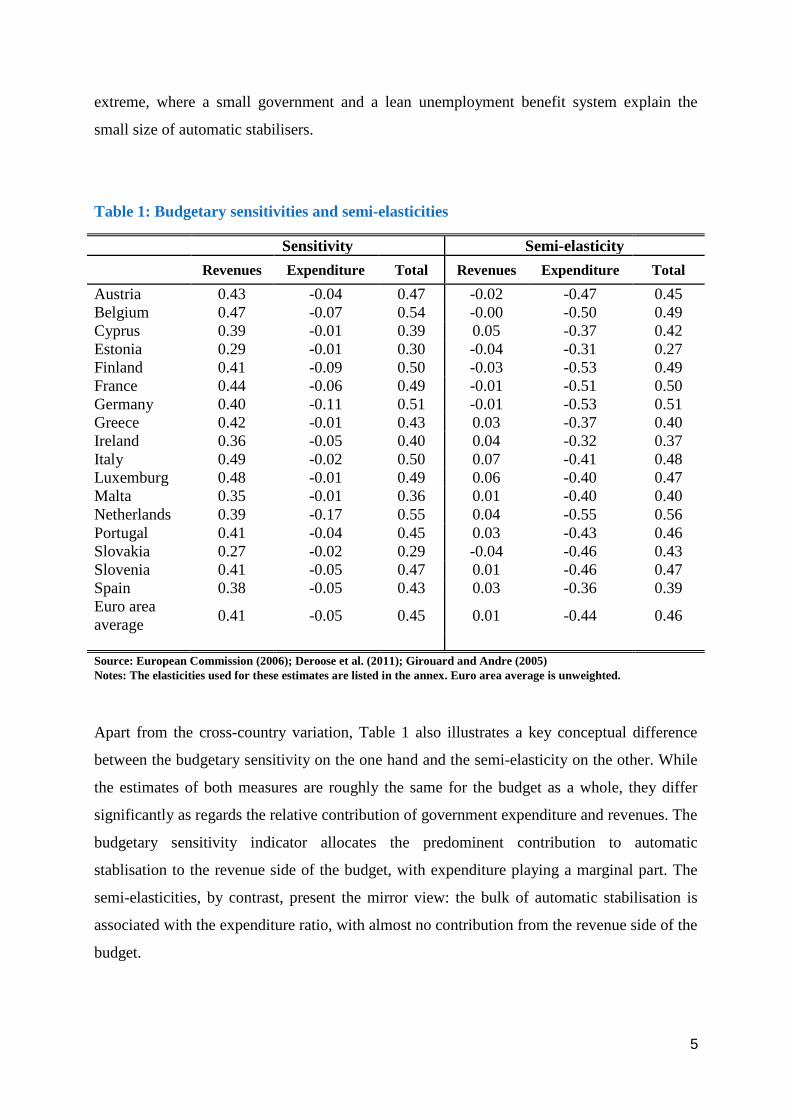
Tabl;e 1 shows empirical estimates of the budgetary sensitivities and semi-elasticities of the

Euro area and the participating EU member states.

The cross-country differences in the estimates reflect an number of factors, notably the degree

of progressivity of the tax system, the importance of unemployment benefits, and the size of

government as measured by the government revenue and expenditure ratio R/Y and G/Y. In

the case of Germany, for instance, the relatively large estimates are due to the comparatively

large size of government. In the case of the Netherlands it is a combination of both the size of

government and the relative importance of unemployment benefits. Ireland represent the other

5

extreme, where a small government and a lean unemployment benefit system explain the

small size of automatic stabilisers.

Table 1: Budgetary sensitivities and semi-elasticities

Sensitivity Semi-elasticity Revenues Expenditure Total Revenues Expenditure Total Austria 0.43 -0.04 0.47 -0.02 -0.47 0.45 Belgium 0.47 -0.07 0.54 -0.00 -0.50 0.49 Cyprus 0.39 -0.01 0.39 0.05 -0.37 0.42 Estonia 0.29 -0.01 0.30 -0.04 -0.31 0.27 Finland 0.41 -0.09 0.50 -0.03 -0.53 0.49 France 0.44 -0.06 0.49 -0.01 -0.51 0.50 Germany 0.40 -0.11 0.51 -0.01 -0.53 0.51 Greece 0.42 -0.01 0.43 0.03 -0.37 0.40 Ireland 0.36 -0.05 0.40 0.04 -0.32 0.37 Italy 0.49 -0.02 0.50 0.07 -0.41 0.48 Luxemburg 0.48 -0.01 0.49 0.06 -0.40 0.47 Malta 0.35 -0.01 0.36 0.01 -0.40 0.40 Netherlands 0.39 -0.17 0.55 0.04 -0.55 0.56 Portugal 0.41 -0.04 0.45 0.03 -0.43 0.46 Slovakia 0.27 -0.02 0.29 -0.04 -0.46 0.43 Slovenia 0.41 -0.05 0.47 0.01 -0.46 0.47 Spain 0.38 -0.05 0.43 0.03 -0.36 0.39 Euro area average 0.41 -0.05 0.45 0.01 -0.44 0.46 Source: European Commission (2006); Deroose et al. (2011); Girouard and Andre (2005) Notes: The elasticities used for these estimates are listed in the annex. Euro area average is unweighted.

Apart from the cross-country variation, Table 1 also illustrates a key conceptual difference

between the budgetary sensitivity on the one hand and the semi-elasticity on the other. While

the estimates of both measures are roughly the same for the budget as a whole, they differ

significantly as regards the relative contribution of government expenditure and revenues. The

budgetary sensitivity indicator allocates the predominent contribution to automatic

stablisation to the revenue side of the budget, with expenditure playing a marginal part. The

semi-elasticities, by contrast, present the mirror view: the bulk of automatic stabilisation is

associated with the expenditure ratio, with almost no contribution from the revenue side of the

budget.

6

This difference is of course implied by the way the two indicators are defined: one looks at

changes in levels, the other at changes in ratios to GDP. At the same time, the definitions also

embody different views about a budget in which automatic stabilisers are not allowed to work,

that is, a view about a counterfactual budget without automatic stabilisers. By focusing on

changes in levels, budgetary sensitivities implicitly assume that without build-in automatic

stabilisers budgetary components would remain constant in levels. By focusing on ratios to

GDP, semi-elasticities presume a neutral budget whereby expenditure and revenues remain

proportional with respect the variable that is expected to be stabilised notably GDP. As such,

different benchmark budgets will also imply different sources of automatic stabilisation.

3. What is the counterfactual to automatic stabilisers?

When evaluating the effectiveness of automatic stabilisers, as measured by the degree of

output smoothing produced by the built-in budgetary elements, one has to compare the

outcome with a situation where the automatic stabilisers are "switched off".

The fact that many different views on the nature of automatic stabilisers prevail in the

literature shows that, until now, no general benchmark has been established. In general, we

can distinguish between two types of benchmark budgets, matching the two indicators of the

size of automatic stabilisers discussed in the previous section: the first entails keeping the

levels of government expenditure and revenues fixed, while in the second government

expenditure and revenues vary with GDP so as to keep their ratio constant.

Table 2 gives an overview of a selection of key papers on automatic stabilisers. For each

paper the estimated degree of output smoothing is reported, together with the assumed

benchmark budget.

As can be seen in Table 2, both types of benchmark budgets are used in the literature. The

exact configuration of the neutral budget, however, varies significantly. Most papers in the

relevant literature do not explicitly define the benchmark or counterfactual budget. In most

cases, however, upon careful reading, the benchmark can be inferred.

7

Table 2: Degree of output smoothing - Overview of literature

Paper

Sample Output smoothing Benchmark budget

Auerbach and Feenberg (2000)

US 8% Lump sum revenues

Cohen and Follette (2000)

US 10% Fixed level of revenues

Van den Noord (2000)

19 OECD countries

25% Fixed ratios of revenues and expenditure

Buti et al. (2002) Belgium 14% Fixed ratio of fiscal balance France 22%

Meyermans (2002) Euro Area 11% Fixed deficit-to-GDP ratio US 20%

Barrell et al. (2002) Euro area 9% Fixed levels of revenues and expenditure

Brunilla et al. (2003) EU Consumption shock: 20-30%

fixed level of fiscal balance

Private investment shock: 3-10%

Barrell and Pina (2004)

Euro area 11% Fixed levels of revenues and expenditure

Tödter et Scharnagl (2004)

Germany Consumption shock: 18-26%

Fixed level of fiscal balance

Investment shock: 10-15% Follette and Lutz (2010)

US 10% after 4 quarters, 20% after 8 quarters

fixed levels of revenues and expenditure

Dolls et al. (2012) US vs Europe

Income shock: 4-22% (EU); 6-17% (US)

Lump sum revenues and expenditure

Unemployment shock: 13-30% (EU); 7-20% (US)

The very early literature on automatic stabilisation, best represented by Musgrave and Miller

(1948), mostly uses a benchmark where both revenue and expenditure are fixed in absolute

values. A similar assumption is used by Auerbach and Feenberg (2000) who define the

stabilising effect of taxes as compared to a situation in which taxes are of a lump sum type,

and hence do not affect disposable income in case of cyclical fluctuations. Many other

researchers have followed variations of this approach. For instance, Barrel et al. (2002) who

fix taxes and spending at the level implied by their 'structural rate'. The same method is used

by Barrel and Pina (2004). Cohen and Follette (2000) set each tax rate to zero in the

benchmark and introduce an add factor that sets tax receipts equal to their baseline values.

8

Brunila et al. (2003) define the benchmark budget as one where the impact of economic

fluctuations is offset by across-the-board changes in other budget items, so as to keep the

overall fiscal balance constant. Tödter and Scharnagl (2004) use three different methods to

keep the level of budget balance fixed in the benchmark: exogenisation of the budget

components, revenue compensation and expenditure compensation. Contrary to the

exogenisation approach, the compensation approach lets automatic stabilisers active, but

compensates their effect by discretionary changes in revenues or expenditure. Follette and

Lutz (2010) define the benchmark as the case where taxes are independent of income and

transfers are independent of the unemployment rate, which implies that the level of taxes and

transfers is kept constant. Following the basic approach of Auerbach and Feenberg (2000),

Dolls et al. (2012) implicitly assume that in the benchmark budget revenues and transfers are

of a lump sum type.

Van den Noord (2000), by contrast sets taxes and spending equal to their structural rate, as a

constant share of GDP. Buti et al. (2002) require for their benchmark that the primary fiscal

balance as a percentage of GDP always stays at its baseline level. Meyermans (2002) keeps

the deficit-to-GDP ratio constant in every period, by adjusting the direct labour income tax

rate.

Views about the nature of a neutral budget are also to be found in studies not directly linked

to the idea of automatic stabilisers. While there is a common understanding that, under

unchanged policies, government revenues broadly follows output, the situation is less clear as

regards a neutral expenditure path. In an attempt to seperate discretionary and automatic

elements in the budget, Buti and Van den Noord (2003) define neutral expenditure as

expenditure that moves in proportion with potential output plus expected inflation. Fatás et al.

(2003) consider three different definitions of a neutral spending path: government spending is

held constant in volume terms; government expenditure grows in line with revenues;

government expenditure grows in proportion with trend GDP. The ambiguity concerning

neutral government expenditure as opposed to the clear view on revenues mirrors the very

nature of the main budgetary items. While tax codes unambiguously link tax revenues to

different forms of income, which in turn are more or less synchronised with total GDP, no

such clear relation can be established for discretionary expenditure.

On the face of it, a discussion about different views concerning the appropriate benchmark

budget might seem rather futile if not completely irrelevant, since by their very nature,

9

automatic stabilisers do their job of output stabilisation irrespective of whether economists

understand their mechanics or not. However, when the actual effectiveness of the stabilisers is

to be evaluated, the benchmark has to be made explicit. The lack of a commonly agreed view

on what a neutral budget looks like, can partly be explained by the fact that, apart from

unemployment benefits, automatic stabilisation is largely the welcome but unintentional effect

of budgetary arrangements that were designed to serve other purposes: progressive taxation is

primarily motivated by distributional considerations; different sizes of government reflect

different views about the reflective merits of private versus public provisions of goods and

services; and unemployment benefits can be motivated by both social and efficiency

considerations.

As hinted at above, the choice of the benchmark determines the narrative about the origin of

automatic stabilisation. Those who define a neutral budget as a budget where expenditure and

revenues are fixed in levels, see changes in the level of taxation and unemployment benefits

as automatically stabilising. Since unemployment benefits are relatively small, the bulk of

stabilisation is associated with the revenue side of the budget. If the benchmark budget is

defined as one where revenue and expenditure are constant as share of GDP, automatic

stabilisations mainly stems from progressive taxation and the size of government, notably

from the fact that the bulk of government expenditure does not respond to cyclical

fluctuations. The difference is particularly clear in the case of proportional taxation:

proportional taxes can only be taken to produce a stabilising effect on output if in the

benchmark budget revenues are fixed in levels. A similar reasoning applies to discretionary

spending. The inertia of government spending, in particular wages and transfers, can only

produce a stabilising effect of total output if in the neutral budget government expenditure is

taken to follow GDP.

4. Degree of output smoothing of automatic stabilisers

4.1 Empirical estimates in literature

The most common method to estimate the effect of automatic stabilisers is the use of

simulation models. As was already highlighted in Table 2, previous estimates in the literature

vary significantly. Cohen and Follette (2000) conclude that in the US built-in stabilisers

smooth output fluctuations by about 10 per cent,while Follette and Lutz (2010) find a

10

stabilisation of approximately 10 per cent after four quarters and 20 per cent after eight

quarters. Also for the US, Auerbach and Feenberg (2000) estimate that automatic stabilsers

offset about 8 per cent of cyclical output fluctuations. Simulations by OECD (Van den Noord,

2000) indicate a degree of smoothing of on average a quarter during the 1990s in 19 OECD

member countries. Meyermans (2002) finds that GDP stabilisation after a demand shock

equals about 11 per cent in the euro area and 20 per cent in the US. For the Euro area Barrel et

al. (2002) estimate stabilisation gains at 9 per cent when considering only taxes and

unemployment benefits. Barrell and Pina (2004) estimate these gains at 11 per cent. By

contrast, Dolls et al. (2012) find that automatic stabilizers give rise to a demand stabilization

for income shocks of 4 to 22 per cent in the EU, depending on the share of liquidity

constraints, and 6 to 17 per cent in the US, with large differences between the EU countries.

Brunilla et al. (2003) emphasise the fact that the effectiveness of automatic stabilisers depends

on the type of shock to the economy. They estimate that in the Eurozone about 20 to 30 per

cent of a private consumption shock is smoothed by taxes and unemployment benefits,

whereas this is only 3 to 10 per cent for a private investment shock. The importance of the

type of shock is confirmed by Tödter and Scharnagl (2004), who find that in Germany, the

Netherlands, France, UK, Italy, Japan and the US, a consumption shock is better smoothed

than other demand shocks. Smoothing power is more or less the same in these countries,

except for Japan where automatic stabilisers are found to be significantly more effective.

The substantial differences in these estimates can be explained by the use of different

simulation methods, but also by different definitions of automatic stabilisers and, linked to

that, of benchmark budgets. Outcomes that are based on different understandings of the

concept of automatic stabilisers cannot be compared properly.

At this stage it may be useful to recall that automatic stabilisers only work with temporary

demand and supply shocks. They may lead to unsustainable levels of government spending

and taxation in the case of a permanent supply shocks. A permanent supply shock requires

adjustment to the new equilibrium rather than output stabilisation. In fact, automatic

stabilisation will in this case only slow down the adjustment process (Buti and Franco,

2005).2

2 Given the uncertainty about the temporary or permanent nature of shocks, strong automatic stabilisers may therefore not always be desirable. In the same spirit, there could be potential conflicts between automatic stabilisation and structural reforms.

11

4.2 Simulations with the QUEST model

In order to show the importance of defining a proper benchmark budget, we run model

simulations with the European Commission's QUEST model, of which details are provided in

the Annex.

We first simulate different types of economic shocks for two alternative benchmark budgets.

The results of these benchmark simulations are then compared to a configuration where the

same shocks are sent through the model in which automatic stabilisers are switched on.

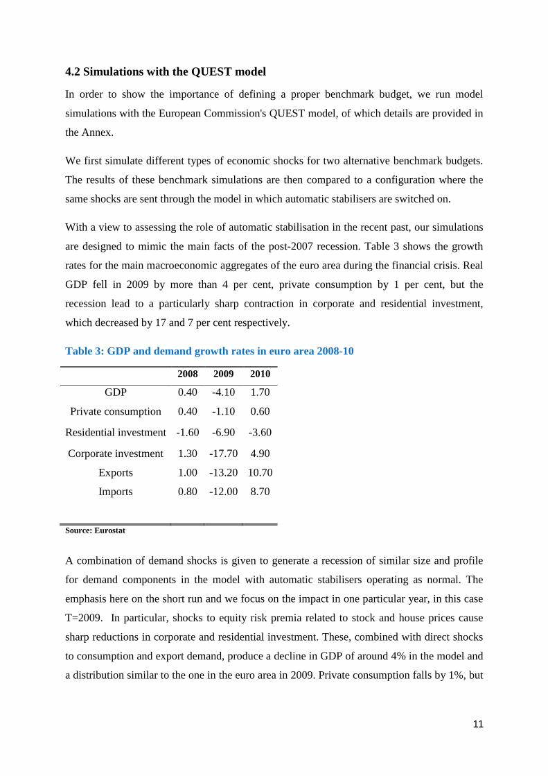
With a view to assessing the role of automatic stabilisation in the recent past, our simulations

are designed to mimic the main facts of the post-2007 recession. Table 3 shows the growth

rates for the main macroeconomic aggregates of the euro area during the financial crisis. Real

GDP fell in 2009 by more than 4 per cent, private consumption by 1 per cent, but the

recession lead to a particularly sharp contraction in corporate and residential investment,

which decreased by 17 and 7 per cent respectively.

Table 3: GDP and demand growth rates in euro area 2008-10

2008 2009 2010

GDP 0.40 -4.10 1.70

Private consumption 0.40 -1.10 0.60

Residential investment -1.60 -6.90 -3.60

Corporate investment 1.30 -17.70 4.90

Exports 1.00 -13.20 10.70

Imports 0.80 -12.00 8.70

Source: Eurostat

A combination of demand shocks is given to generate a recession of similar size and profile

for demand components in the model with automatic stabilisers operating as normal. The

emphasis here on the short run and we focus on the impact in one particular year, in this case

T=2009. In particular, shocks to equity risk premia related to stock and house prices cause

sharp reductions in corporate and residential investment. These, combined with direct shocks

to consumption and export demand, produce a decline in GDP of around 4% in the model and

a distribution similar to the one in the euro area in 2009. Private consumption falls by 1%, but

12

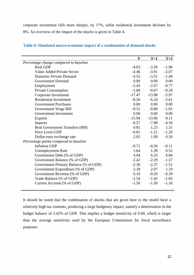
corporate investment falls more sharply, by 17%, while residential investment declines by

8%. An overview of the impact of the shocks is given in Table 4.

Table 4: Simulated macro-economic impact of a combination of demand shocks

T T+1 T+2 Percentage change compared to baseline

Real GDP -4.03 -3.59 -1.96 Value Added Private Sector -4.46 -3.91 -2.07 Domestic Private Demand -4.55 -3.51 -1.49 Government Demand 0.00 0.00 0.00 Employment -2.43 -2.07 -0.77 Private Consumption -1.00 -0.67 -0.28 Corporate Investment -17.47 -13.98 -5.97 Residential Investment -8.26 -6.24 -2.61 Government Purchases 0.00 0.00 0.00 Government Wage Bill -0.31 -0.80 -1.01 Government Investment 0.00 0.00 0.00 Exports -15.94 -13.96 -9.11 Imports -9.57 -7.98 -4.56 Real Government Transfers (HH) 0.81 1.23 1.31 Price Level GDP -0.81 -1.21 -1.29 Dollar-euro exchange rate 2.02 1.09 0.10

Percentage points compared to baseline Inflation GDP -0.71 -0.26 -0.11 Unemployment Rate 1.64 1.39 0.52 Government Debt (% of GDP) 4.04 6.33 6.84 Government Balance (% of GDP) -2.42 -2.29 -1.57 Government Primary Balance (% of GDP) -2.36 -2.37 -1.51 Government Expenditure (% of GDP) 2.39 2.07 1.19 Government Revenue (% of GDP) 0.10 -0.20 -0.39 Trade Balance (% of GDP) -1.54 -1.42 -1.05 Current Account (% of GDP) -1.56 -1.50 -1.16

It should be noted that the combination of shocks that are given here to the model have a

relatively high tax contents, producing a large budgetary impact, namely a deterioration in the

budget balance of 2.42% of GDP. This implies a budget sensitivity of 0.60, which is larger

than the average sensitivity used by the European Commission for fiscal surveillance

purposes.

13

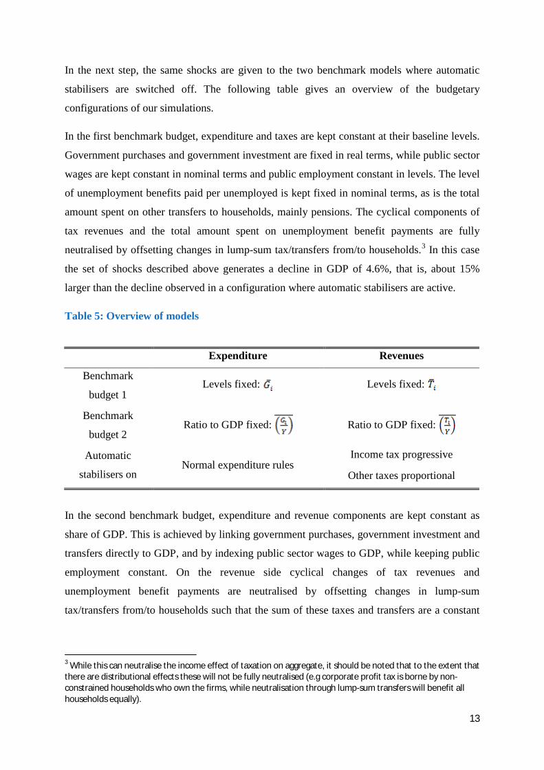
In the next step, the same shocks are given to the two benchmark models where automatic

stabilisers are switched off. The following table gives an overview of the budgetary

configurations of our simulations.

In the first benchmark budget, expenditure and taxes are kept constant at their baseline levels.

Government purchases and government investment are fixed in real terms, while public sector

wages are kept constant in nominal terms and public employment constant in levels. The level

of unemployment benefits paid per unemployed is kept fixed in nominal terms, as is the total

amount spent on other transfers to households, mainly pensions. The cyclical components of

tax revenues and the total amount spent on unemployment benefit payments are fully

neutralised by offsetting changes in lump-sum tax/transfers from/to households.3 In this case

the set of shocks described above generates a decline in GDP of 4.6%, that is, about 15%

larger than the decline observed in a configuration where automatic stabilisers are active.

Table 5: Overview of models

Expenditure Revenues

Benchmark

budget 1 Levels fixed: Levels fixed:

Benchmark

budget 2 Ratio to GDP fixed: Ratio to GDP fixed:

Automatic

stabilisers on Normal expenditure rules

Income tax progressive

Other taxes proportional

In the second benchmark budget, expenditure and revenue components are kept constant as

share of GDP. This is achieved by linking government purchases, government investment and

transfers directly to GDP, and by indexing public sector wages to GDP, while keeping public

employment constant. On the revenue side cyclical changes of tax revenues and

unemployment benefit payments are neutralised by offsetting changes in lump-sum

tax/transfers from/to households such that the sum of these taxes and transfers are a constant

3 While this can neutralise the income effect of taxation on aggregate, it should be noted that to the extent that there are distributional effects these will not be fully neutralised (e.g corporate profit tax is borne by non-constrained households who own the firms, while neutralisation through lump-sum transfers will benefit all households equally).

14

share of GDP. In this case the composite shock defined above gives rise to a drop in GDP of

5.5%, which is about 36% larger than the drop recorded with built-in stabilisers on.

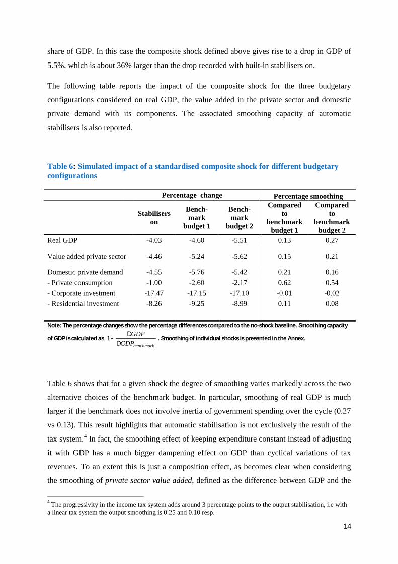
The following table reports the impact of the composite shock for the three budgetary

configurations considered on real GDP, the value added in the private sector and domestic

private demand with its components. The associated smoothing capacity of automatic

stabilisers is also reported.

Table 6: Simulated impact of a standardised composite shock for different budgetary configurations

Table 6 shows that for a given shock the degree of smoothing varies markedly across the two

alternative choices of the benchmark budget. In particular, smoothing of real GDP is much

larger if the benchmark does not involve inertia of government spending over the cycle (0.27

vs 0.13). This result highlights that automatic stabilisation is not exclusively the result of the

tax system.4 In fact, the smoothing effect of keeping expenditure constant instead of adjusting

it with GDP has a much bigger dampening effect on GDP than cyclical variations of tax

revenues. To an extent this is just a composition effect, as becomes clear when considering

the smoothing of private sector value added, defined as the difference between GDP and the

4 The progressivity in the income tax system adds around 3 percentage points to the output stabilisation, i.e with a linear tax system the output smoothing is 0.25 and 0.10 resp.

Percentage change Percentage smoothing

Stabilisers on

Bench-mark

budget 1

Bench- mark

budget 2

Compared to

benchmark budget 1

Compared to

benchmark budget 2

Real GDP -4.03 -4.60 -5.51 0.13 0.27

Value added private sector -4.46 -5.24 -5.62 0.15 0.21

Domestic private demand -4.55 -5.76 -5.42 0.21 0.16 - Private consumption -1.00 -2.60 -2.17 0.62 0.54 - Corporate investment -17.47 -17.15 -17.10 -0.01 -0.02 - Residential investment -8.26 -9.25 -8.99 0.11 0.08

Note: The percentage changes show the percentage differences compared to the no-shock baseline. Smoothing capacity

of GDP is calculated as benchmarkGDP

GDPD

D-1 . Smoothing of individual shocks is presented in the Annex.

15

government wage bill. The difference in smoothing between the two benchmarks for this

measure is much smaller, only 0.06, suggesting a significant part of the smoothing in total

GDP stems from the valuation of general government output. 5

When looking at domestic private demand, we see that smoothing under the first benchmark

is higher. Automatic stabilisers are more effective in stabilising total domestic demand in the

fixed levels benchmark. Private consumption is most smoothed by the automatic stabilisers,

as stabilisation mainly operates on households disposable incomes, and keeping transfers

constant in levels stabilises incomes. The degree of smoothing of consumption obviously

depends on the share of liquidity-constrained and credit-constrained households, which

amount to 40 percent in total in the model calibration. Consumption smoothing will be higher

if this share is larger. Interestingly, automatic stabilisers have no impact on corporate

investment. Investment decisions in the model are determined by the net present value of

investment projects over their whole lifetime, and automatic stabilisers have no impact on

this. In fact, there is a small increase in variability in investment, a general equilibrium effect

due to higher real interest rates as consumption is smoothed by the operation of automatic

stabilisers. Residential investment on the other hand is partly smoothed to the extent that

credit constrained households' disposable income is affected by the automatic stabilisers.

How does the estimated output smoothing from automatic stabilisers compare to estimates of

budget sensitivities and fiscal multipliers ? Fiscal multipliers for temporary shocks in the

model are close to or slightly above 1 for government consumption and investment shocks,

but significantly smaller for transfer shocks (around 0.4). Multipliers for tax shocks are also

generally smaller, between 0.2 and 0.5 for labour and consumption taxes and close to zero for

corporate taxes. 6 The average multiplier for fiscal shocks operating on household disposable

income is around 0.4. With a budget sensitivity of 0.6 this would imply a GDP smoothing of

around 0.24, close to the estimates reported in this section.

5 In the absence of better productivity measures, general government output is valued at costs, and changes in government wages affect GDP and value added not only in nominal terms but also in volume terms. 6 Roeger and in 't Veld (2010), p. 23. See also Coenen et al (2012) for comparable multipliers in structural models of other international organisations.

16

5. Summary and conclusions

As the euro-area member states cannot take individual monetary actions to stabilise their

economies, and since the Stability and Growth Pact (and in the future the new fiscal compact)

limits discretionary fiscal policy, knowing the size and effect of automatic stabilisers is

particularly relevant in the EU. When determining the effect of automatic stabilisers, a

benchmark budget has to be defined against which the degree of smoothing is to be measured.

Earlier work on automatic stabilisation typically failed to be explicit about the type of

benchmark budget used or considered only one type of benchmark.

With a view to illustrating the importance of the benchmark budget, in this paper we first

clarify a number of conceptual issues and run simulations with the European Commission's

QUEST model. For that purpose, two different benchmarks budgets were defined: one where

the levels of both expenditure and revenues are held constant and a second that keeps the ratio

of expenditure and revenues to GDP fixed. When using the fixed level benchmark the bulk of

stabilisation comes from taxes and unemployment benefits, while for the fixed ratios

benchmark the main sources of stabilisation is the size of government.

Our simulation of shocks that closely capture the main stylised facts of the 2008-9 recession

shows that the degree of stabilisation is fairly significant, and more importantly, that it differs

markedly across benchmarks. Our results indicate that automatic stabilisers could have ironed

out 13 per cent of the drop of GDP in the euro area compared to a benchmark budget with

fixed levels of revenues and expenditure. The degree of smoothing increases to 27 per cent

when using a benchmark where revenues and expenditure follow GDP. Hence, dampening of

cyclical fluctuations through the inertia of discretionary spending largely exceeds the

smoothing effect of tax revenues.

17

Bibliography

Auerbach, A., & Feenberg, D. (2000). The Significance of Federal Taxes as Automatic

Stabilizers. NBER Working Papers No. 7662.

Barrell, R., Hurst, I., & Pina, A. (2002). Fiscal Targets, Automatic Stabilisers and Their

Effects on Output. NIESR working paper.

Barrell, R., & Pina, A. (2004). How Important are Automatic Stabilisers in Europe? A

Stochatic Simulation Assessment. Economic Modelling, Elsevier, Vol. 21, No. 1: 1-35.

Blinder, A. S. (2004). The Case Against the Case Against Discretionary Fiscal Policy. CEPS

Working Paper No. 102.

Brunila, A., Buti, M., & In't Veld, J. (2003). Fiscal Policy in Europe: How Effective are

Automatic Stabilisers? Empirica, Vol. 30: 1-24.

Buti, M., & Franco, D. (2005). Fiscal policy in Economic and Monetary Union: theory,

evidence, and institutions. Cheltenham: Edward Elgar Publishing.

Buti, M., & Van den Noord, P. (2003). Discretionary Fiscal Policy and Elections: The

Experience of the Early Years of EMU. OECD Economics Department Working

Papers no. 351.

Buti, M., Martinez-Mongay, C., Sekkat, K., & van den Noord, P. (2002). Automatic

Stabilisers and Market Flexibility in the EMU - Is there a trade-off? OECD Economics

Department Working Papers no. 335.

Christiano, L., M. Eichenbaum, and S.Rebelo. 2011. “When Is the Government Spending

Multiplier Large?” Journal of Political Economy, Vol. 119, No. 1: 78–121.

Coenen, G., C. Erceg, C. Freedman, D. Furceri, M. Kumhof, R. Lalonde, D. Laxton, J. Linde,

A. Mourougane, D. Muir, S. Mursula, C. de Resende, J. Roberts, W. Roeger, S.

Snudden. M. Trabandt, J. in ’t Veld (2012). Effects of Fiscal Stimulus in Structural

Models. American Economic Journal: Macroeconomics, Vol. 4, No. 1: 22-68,

available at: http://pubs.aeaweb.org/doi/pdfplus/10.1257/mac.4.1.22

18

Cogan, J.F., T. Cwik, J.B. Taylor, and V. Wieland. 2010. “New Keynesian versus Old

Keynesian Government Spending Multipliers.” Journal of Economic Dynamics and

Control, Vol. 34, No. 3:281–95.

Cohen, D., & Follette, G. (2000). The Automatic Fiscal Stabilizers: Quietly Doing Their

Thing. Federal Reserve Bank of New York Economic Policy Review 6, 35-68.

Davig,T.,and E.M.Leeper (2011): “Monetary-Fiscal Policy Interactions and Fiscal Stimulus,”

European Economic Review, Vol. 55, No. 2: 211–227.

.Deroose, S., Larch, M., & Schachter, A. (2011). Constricted, lame and pro-cyclical? Fiscal

policy in the euro area revisited. International Journal of Sustainable Economy, Vol.

3, No. 2 : 162 - 184.

Dolls, M., Fuest c & Peichl, A. (2012) Automatic stabilisers and economic crisis: US vs. Europe, Journal of Public Economics, Vol. 96, 279-294.

European Commisison (2001). Public Finances in the EMU. European Economy, Brussels..

European Commission (2006). Public Finances in EMU. European Economy, Brussels.

Fatás, A., & Mihov, I. (2001). Government Size and Automatic Stabilisers:

International and Intranational Evidence. Journal of International Economics, Vol. 55,

Nr. 1: 3-28.

Fatás, A., Von Hagen, J., & Hughes Hallett, A. (2003). Stability and Growth in Europe:

Towards a Better Pact. Centre for Economic Policy Research.

Follette, G., & Lutz, B. (2010). Fiscal Policy in the United States: Automatic Stabilisers,

Discretionary Fiscal Policy Actions, and the Economy. 12th Banca d'Italia Public

Finance Workshop. Perugia.

Girouard, N. & C. André (2005). Measuring cyclically-adjusted budget balances for OECD

countries, Economics Department Working Paper No.434.

Hajdenberg, A., J. A. del Granado & S. Gupta (2010). "Is Social Spending Procyclical?," IMF

Working Papers 10/234, International Monetary Fund.

Hemming, R., Kell, M., & Mahfouz, S. (2002). The Effectiveness of Fiscal Policy in

Stimulating Economic Activity - A Review of the Literature. IMF Working Papers

No. 02/208.

19

Lee, Y., & Sung, T. (2007). Fiscal Policy, Business Cycles and Economic Stabilisation:

Evidence from Industrialised and Developing Countries. Fiscal Studies, Vol. 28, No.

4: 437-462.

Melitz, J., & Darby, J. (2008). Social spending and automatic stabilizers in the OECD.

Economic Policy, 715-756.

Meyermans, E. (2002). Automatic Fiscal Stabilisers in the Euro Area: Simulations with the

NIME model'. Fourth Workshop on Public Finance. Perugia: Banca d'Italia.

Musgrave, R., & Miller, M. (1948). Built-in Flexibility. The American Economic Review,

Vol.38, No. 1: 122-128.

Ratto, M., Roeger, W., & in 't Veld, J. (2009). QUEST III: An estimated open-economy

DSGE model of the euro area with fiscal and monetary policy. Economic Modelling,

Elsevier, Vol. 26, No. 1: 222-233.

Rodrik, D. (1998). Why Do More Open Economies Have Bigger Governments? Journal of

political Economy, Vol. 106: 997-1032.

Roeger W., in 't Veld J. (2010), “Fiscal stimulus and exit strategies in the EU: a model-based

analysis", European Economy Economic Papers No. 426. Available at: http://ec.europa.eu/economy_finance/publications/economic_paper/2010/pdf/ecp426_en.pdf

Taylor, J. B. (2009). The Lack of an Empirical Rationale for a Revival of Discretionary Fiscal

Policy American Economic Review, Vol. 99, No. 2: 550–55.

Tödter, K.-H., & Scharnagl, M. (2004). How effective are automatic stabilisers? Theory and

empirical results for Germany and other OECD countries. Deutsche Bundesbank

Discussion Paper, 21.

Van den Noord, J. (2000). The Size and Role of Automatic Fiscal Stabilizers in the 1990s and

Beyond. OECD Economics Department Working Papers No.230.

20

Annex

The QUEST simulation model

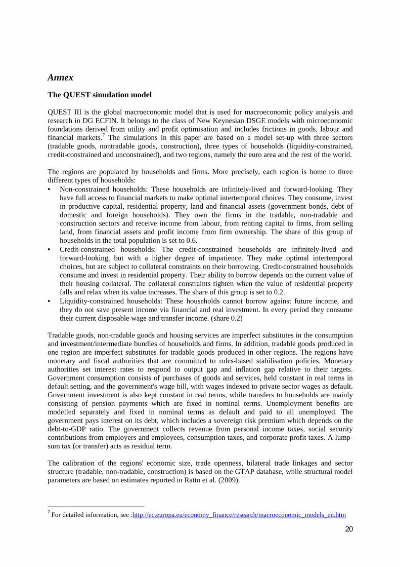
QUEST III is the global macroeconomic model that is used for macroeconomic policy analysis and research in DG ECFIN. It belongs to the class of New Keynesian DSGE models with microeconomic foundations derived from utility and profit optimisation and includes frictions in goods, labour and financial markets.7 The simulations in this paper are based on a model set-up with three sectors (tradable goods, nontradable goods, construction), three types of households (liquidity-constrained, credit-constrained and unconstrained), and two regions, namely the euro area and the rest of the world. The regions are populated by households and firms. More precisely, each region is home to three different types of households: · Non-constrained households: These households are infinitely-lived and forward-looking. They

have full access to financial markets to make optimal intertemporal choices. They consume, invest in productive capital, residential property, land and financial assets (government bonds, debt of domestic and foreign households). They own the firms in the tradable, non-tradable and construction sectors and receive income from labour, from renting capital to firms, from selling land, from financial assets and profit income from firm ownership. The share of this group of households in the total population is set to 0.6.

· Credit-constrained households: The credit-constrained households are infinitely-lived and forward-looking, but with a higher degree of impatience. They make optimal intertemporal choices, but are subject to collateral constraints on their borrowing. Credit-constrained households consume and invest in residential property. Their ability to borrow depends on the current value of their housing collateral. The collateral constraints tighten when the value of residential property falls and relax when its value increases. The share of this group is set to 0.2.

· Liquidity-constrained households: These households cannot borrow against future income, and they do not save present income via financial and real investment. In every period they consume their current disposable wage and transfer income. (share 0.2)

Tradable goods, non-tradable goods and housing services are imperfect substitutes in the consumption and investment/intermediate bundles of households and firms. In addition, tradable goods produced in one region are imperfect substitutes for tradable goods produced in other regions. The regions have monetary and fiscal authorities that are committed to rules-based stabilisation policies. Monetary authorities set interest rates to respond to output gap and inflation gap relative to their targets. Government consumption consists of purchases of goods and services, held constant in real terms in default setting, and the government's wage bill, with wages indexed to private sector wages as default. Government investment is also kept constant in real terms, while transfers to households are mainly consisting of pension payments which are fixed in nominal terms. Unemployment benefits are modelled separately and fixed in nominal terms as default and paid to all unemployed. The government pays interest on its debt, which includes a sovereign risk premium which depends on the debt-to-GDP ratio. The government collects revenue from personal income taxes, social security contributions from employers and employees, consumption taxes, and corporate profit taxes. A lump-sum tax (or transfer) acts as residual term. The calibration of the regions' economic size, trade openness, bilateral trade linkages and sector structure (tradable, non-tradable, construction) is based on the GTAP database, while structural model parameters are based on estimates reported in Ratto et al. (2009).

7 For detailed information, see :http://ec.europa.eu/economy_finance/research/macroeconomic_models_en.htm

21

Table A.1: Revenue and expenditure elasticities

Personal tax

Corporate tax

Indirect taxes

Social contributions

Total revenues

Current expenditure

Austria 1.31 1.69 1.00 0.58 1.00 -0.08 Belgium 1.09 1.57 1.00 0.80 0.99 -0.16 Cyprus 2.10 1.50 1.00 0.70 1.14 -0.02 Estonia 0.80 1.40 1.00 0.70 0.90 -0.05 Finland 0.91 1.64 1.00 0.62 0.92 -0.21 France 1.18 1.59 1.00 0.79 0.98 -0.12 Germany 1.61 1.53 1.00 0.57 0.97 -0.27 Greece 1.80 1.08 1.00 0.85 1.07 -0.04 Ireland 1.44 1.30 1.00 0.88 1.14 -0.16 Italy 1.75 1.12 1.00 0.86 1.17 -0.04 Luxemburg 1.50 1.75 1.00 0.76 1.14 -0.04 Malta 2.20 1.40 1.00 0.40 1.04 -0.02 The Netherlands 1.69 1.52 1.00 0.56 1.01 -0.42

Portugal 1.53 1.17 1.00 0.92 1.08 -0.09 Slovakia 0.70 1.32 1.00 0.70 0.88 -0.04 Slovenia 1.40 1.50 1.00 0.70 0.96 -0.13 Spain 1.92 1.15 1.00 0.68 1.09 -0.16 Euro area average 1.48 1.43 1.00 0.74 1.04 -0.15 Source: Girouard and Andre (2005) and European Commission (2006)

Table A.2: GDP Smoothing capacity for individual shocks

Consumption shock Housing shock Export demand shock

Smoothing compared

to benchmark budget 1 0.17 0.13 0.12

Smoothing compared

to benchmark budget 2 0.32 0.28 0.27