Automatic estimation of the inlier threshold in robust

Automatic estimation of the inlier thresholdin robust multiple structures fitting.

Roberto Toldo and Andrea Fusiello

Dipartimento di Informatica, Universita di VeronaStrada Le Grazie 15, 37134 Verona, Italy

[email protected] [email protected]

Abstract. This paper tackles the problem of estimating the inlier threshold inRANSAC-like approaches to multiple models fitting. An iterative approach findsthe maximum of a score function which resembles the Silhouette index used inclustering validation. Although several methods have been proposed to solve thisproblem for the single model case, this is the first attempt to address multiplemodels. Experimental results demonstrate the performances of the algorithm.

1 Introduction

Fitting multiple models to noisy data is a widespread problem in Computer Vision. Oneof the most successful paradigm that sprouted after RANSAC is the one based on ran-dom sampling. Within this paradigm there are parametric methods (Randomized HoughTransform [1], Mean Shift [2]), and non parametric ones, (RANSAC [3], Residual his-togram analysis [4], J-linkage [5]). In general the latter achieves better performancesthan the former and have a more general applicability, provided that the inlier thresholdε (also called scale), onto which they depend critically, is manually specified.

Some works [6–9] deal with the automatic computation of ε in the case of one model– i.e., in the case of RANSAC – but that are not extendible to the case of multiplemodels. In this paper we aim at filling this gap, namely at estimating ε when using arandom sampling and residual analysis approach to fit multiple instances of a model tonoisy data corrupted by outliers.

If ε is too small, noisy data points are explained by multiple similar well-fittedmodels, that is, the separation of the models is poor; if ε is too large, they are explainedby a single poorly-fitted model, that is, the compactness of the model is poor. The ”justright” ε should strike the balance between model separation and model compactness.

The degree of separation with respect to compactness is measured by a score verysimilar to the Silhouette index [10] for clustering validation. We compute the differ-ence between the second and the first least model distance for each data point. Thescale ε provides a normalizing denominator for the error difference. Consider someperturbation to the ”just right” scale. As ε increases, a model recruits new data points,increasing the first error while decreasing the second error, causing the index to drop.As ε decreases, new models are created, decreasing the second error, causing the indexto drop as well. Therefore, the ”just right” scale is the one that yields the largest overallscore from all the points.

2 Roberto Toldo and Andrea Fusiello

We demonstrate our method in association with a baseline algorithm such as sequen-tial RANSAC – sequentially apply RANSAC and remove the inliers from the data setas each model instance is detected – and with an advanced algorithm such as J-linkage[5], which have been recently demonstrated to have very good performances.

2 Fitting validation

The inlier threshold (or scale) ε is used to define which points belong to which model.A point belongs to a model if its distance from the model is less than ε. The pointsbelonging to the same model form the consensus set of that model. We define the “justright” ε as the smallest value that yields the correct models.

In this Section we shall concentrate on a method for estimating such value basedon validating the output of the robust fitting, which consist in a grouping of data pointsaccording to the model they belong to, plus some points (outliers) that have not beenfitted. The criterion for discarding outliers is described in Sec. 3.

The validation of the fitting is based on the concepts of compactness and separation,drawn from the clustering validation literature. In particular, our method stems from thefollowing observation (see Fig. 1):

– if ε is too small a single structure will be fitted by more than one model, resultingin a low separation between points belonging to different models;

– if ε is too large the points fitted by one model will have a low compactness (or,equivalently, a high looseness), which produces a sub-optimal estimate. As an ex-treme case, different structures might be fitted by a single model.

0 0.2 0.4 0.6 0.8 10

0.1

0.2

0.3

0.4

0.5

0.6

0.7

0.8

0.9

1

0 0.2 0.4 0.6 0.8 10

0.1

0.2

0.3

0.4

0.5

0.6

0.7

0.8

0.9

1

0 0.2 0.4 0.6 0.8 10

0.1

0.2

0.3

0.4

0.5

0.6

0.7

0.8

0.9

1

Fig. 1. From right to left: an optimal fit (according to our score), a fit with a smaller ε and a fitwith a bigger ε. The dotted lines depicts the inlier band of width 2ε.

The “just right” ε has to strike the balance between these two effects. This idea iscaptured by the following index – which resembles the Silhouette index [10] – for agiven point i:

ri =bi − ai

ε(1)

where ai is the distance of i to the model it belongs to (looseness) and bi is the distanceof i to the second closest model (separation). The global score, function of ε, is theaverage of ri over all the points. We claim that the “just right” ε is the one that yields the

Automatic estimation of the inlier threshold in robust multiple structures fitting. 3

maximum global score. Indeed, imagine to start with the “just right” ε. If we decrease it,a new model is created which causes the average separation bi to drop. If ε is increasedsuch that at least one new point is added to the model, this point will increase theaverage looseness ai and decrease the average bi, resulting in a decrease of the score(see Fig. 2). A score with a similar behavior (but slightly worse performances with verysmall ε) is the ratio bi/ai which resembles the ratio matching used in [11].

0 0.1 0.2 0.3 0.4 0.5 0.6 0.7 0.8 0.9 10

0.1

0.2

0.3

0.4

0.5

0.6

0.7

0.8

0.9

1

15

15.5

16

16.5

17

0 0.1 0.2 0.3 0.4 0.5 0.6 0.7 0.8 0.9 10

0.1

0.2

0.3

0.4

0.5

0.6

0.7

0.8

0.9

1

0

1

2

3

4

5

6

7

8

9

Fig. 2. This figure is best viewed in color. The left plot depicts a “good fit”, whereas the right plotdepicts a “bad fit” (the upper structure is fitted by two lines very close to each other). The colorof the points encodes the score values, which are consistently lower in the “bad fit”.

The algorithm for finding the optimal ε is iterative: the fitting algorithm is run sev-eral times with different ε and the value that obtained the higher score is retained.

3 Outliers rejection

Sequential RANSAC and J-linkage – like clustering algorithms – in principle fit all thedata. Bad models must be filtered out a-posteriori. Usually it is assumed that the numberof models is known beforehand, but this assumption is too strong and we prefer not torely on it. Thresholding on the cardinality of the consensus set may be an option, butthis does not work if the number of data points supporting the different model instancesare very different. A better approach would exploit the observation that outliers possessa diffused distribution whereas structures are concentrated. In particular, we used herea robust statistics based on points density.

Let ei be distance of point i to its closest neighbor belonging to the same model.According to the X84 rejection rule [12], the inliers are those points such that

ei < 5.2medi |ei −medj ej |. (2)

where med is the median. The models that are supported by the majority of outliersare discarded. Points that are classified as outliers but belongs to a “good” model areretained.

As the robust fit algorithm is executed repeatedly in order to estimate the best ε, themodels that are fitted change, and hence changes the inlier/outlier classification.


0 0.2 0.4 0.6 0.8 10

0.1

0.2

0.3

0.4

0.5

0.6

0.7

0.8

0.9

1

(a) Seq. RANSAC optimalconfiguration.

0 0.2 0.4 0.6 0.8 10

0.1

0.2

0.3

0.4

0.5

0.6

0.7

0.8

0.9

1

(b) J-Linkage optimal con-figuration.

0.05 0.1 0.15 0.2 0.25 0.3 0.35Scale

J−LinkageSeq. RANSAC

(c) Score for different ε val-ues.

Fig. 3. Two lines example.

0 0.2 0.4 0.6 0.8 10

0.1

0.2

0.3

0.4

0.5

0.6

0.7

0.8

0.9

1


0 0.2 0.4 0.6 0.8 10

0.1

0.2

0.3

0.4

0.5

0.6

0.7

0.8

0.9

1


0.05 0.1 0.15 0.2 0.25 0.3 0.35Scale



Fig. 4. Four lines example.

4 Localized sampling

The assumption that outliers posses a diffused distribution implies that the a-prioriprobability that two points belong to the same structure is higher the smaller the dis-tance between the points [13]. Hence minimal sample sets are constructed in a way thatneighboring points are selected with higher probability. This increases the probabilityof selecting a set of inliers [13, 5]. Namely, if a point xi has already been selected, thenxj has the following probability of being drawn:

P (xj |xi) =

{1Z exp− ||xj−xi||2

σ2 if xj 6= xi

0 if xj = xi

(3)

where Z is a normalization constant and σ is chosen heuristically. Given an estimateα of the average inlier-inlier distance, the value of σ is selected such that a point at adistance α has a given probability P to be selected (we set P = 0.5).

σ =α√

−log(P )− log(Z). (4)

The value of α is iteratively estimated as the outlier/inlier classification changes.The normalization constant can be approximated as:

Z ' (1−δ)e−ω2

σ2 + δe−α2

σ2 (5)


where ω is the average inlier-outlier distance and δ is the lowest inlier fraction amongthe models.

The required number of samples that give a desired confidence of success is derivedin [5].

5 Summary of the method

The method that we propose can be seen as a meta-heuristic that is able to set auto-matically all the thresholds, perform outlier rejection and validate the final fitting. Anyalgorithm based on random sampling, from RANSAC to J-linkage, could fit.

The interval search for ε, [εL, εH] must be specified.

Algorithm 11. Set α = εH, ω = 2α.2. for ε = εH to εL

(a) Compute σ, using α and ω (Eq. 4);(b) Run multiple-models fitting (e.g. sequential RANSAC, J-linkage) using σ for sampling

and ε for consensus;(c) Identify outliers (Sec. 3);(d) Compute the average score (Eq. 1);(e) Compute α, ω;

3. end4. Retain the result with the highest score.

6 Experiments

We tested our scale estimation method with two different multiple models fitting al-gorithm based on random sampling: Sequential RANSAC and J-Linkage. The scale isinitialized to a huge value such that in the first step only one model arises. Subsequentlythe scale is decreased by a constant value. We used the same number of samples gener-ated (10000) for all the experiments.

The examples reported consist of both synthetic and real data. In the synthetic ones(Fig. 3 and Fig. 4) we used two and four lines in the plane, respectively The inlier pointsof the lines are surrounded by 50 pure outliers. Gaussian noise with standard deviationof 0.1 is added to coordinate of each inlier point.

In these experiments our meta-heuristic always proved able to converge toward acorrect solution, provided that the underlying fitting algorithm (namely RANSAC orJ-linkage) produced at least one correct fit.

In the real 3D data example (Fig. 5 and Fig. 6) planes are fitted to a cloud of 3Dpoints produced by a Structure and Motion pipeline [14] fed with images of a castle anda square, respectively.




0 0.2 0.4 0.6 0.8 1 1.2 1.4 1.60

10

20

30

40

50

60

70

80

Scale



Fig. 5. Example of planes fitting in 3D from real data (castle).



0 0.2 0.4 0.6 0.8 1 1.2 1.4 1.6 1.80

5

10

15

20

25

30

35

40

45

Scale



Fig. 6. Example of planes fitting in 3D from real data (square).

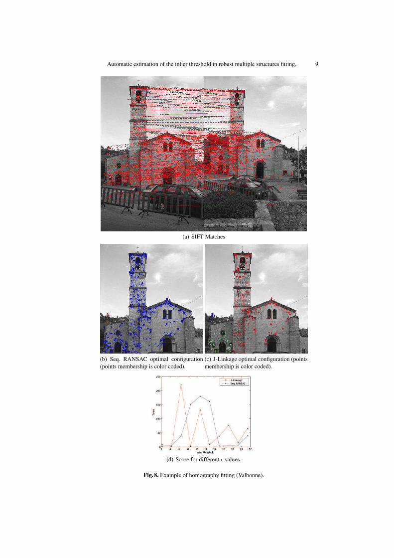
Finally, in the last two datasets (Fig. 7 and Fig. 8), SIFT features [11] are detectedand matched in real images and homographies are fitted to the set of matches.

In the last three cases our scale estimation produced qualitatively different resultswhen applied to sequential RANSAC or J-linkage, as not only the value of the optimalε are different, but also estimated models are different. The J-linkage result is moreaccurate, but the output of sequential RANSAC is not completely wrong, suggestingthat our meta-heuristic is able to produce a sensible result even when applied to a weakalgorithm like sequential RANSAC.

7 Conclusions

In this paper we demonstrated a meta-heuristic for scale estimation in RANSAC-likeapproaches to multiple models fitting. The technique is inspired by clustering valida-tion, and in particular it is based on a score function that resembles the Silhouette index.The fitting results produced by sequential RANSAC or J-linkage with different valuesof scale are evaluated and the best result – according to the score – is retained. Experi-mental results showed the effectiveness of the approach.

Future work will aim at improving the strategy for finding the optimal scale andsmoothly cope with the special case of a single model instance.


References

1. Xu, L., Oja, E., Kultanen, P.: A new curve detection method: randomized Hough transform(RHT). Pattern Recognition Letters 11(5) (1990) 331–338

2. Subbarao, R., Meer, P.: Nonlinear mean shift for clustering over analytic manifolds. In:Proceedings of the IEEE Conference on Computer Vision and Pattern Recognition, York,USA (2006) 1168–1175

3. Fischler, M.A., Bolles, R.C.: Random Sample Consensus: a paradigm model fitting withapplications to image analysis and automated cartography. Communications of the ACM24(6) (June 1981) 381–395

4. Zhang, W., Kosecka, J.: Nonparametric estimation of multiple structures with outliers. In:Workshop on Dynamic Vision, European Conference on Computer Vision 2006. Volume4358 of Lecture Notes in Computer Science., Springer (2006) 60–74

5. Toldo, R., Fusiello, A.: Robust multiple structures estimation with j-linkage. In: ECCV (1).Volume 5302 of Lecture Notes in Computer Science., Springer (2008) 537–547

6. Fan, L., Pylvanainen, T.: Robust scale estimation from ensemble inlier sets for randomsample consensus methods. In: ECCV (3). Volume 5304 of Lecture Notes in ComputerScience., Springer (2008) 182–195

7. Wang, H., Suter, D.: Robust adaptive-scale parametric model estimation for computer vision.IEEE Trans. Pattern Anal. Mach. Intell. 26(11) (2004) 1459–1474

8. Chen, H., Meer, P.: Robust regression with projection based m-estimators. In: In 9th Inter-national Conference on Computer Vision. (2003) 878–885

9. Torr, P.H.S., Murray, D.W.: The development and comparison of robust methods for estimat-ing the fundamental matrix. International Journal of Computer Vision 24(3) (1997) 271–300

10. Rousseeuw, P.: Silhouettes: a graphical aid to the interpretation and validation of clusteranalysis. J. Comput. Appl. Math. 20(1) (1987) 53–65

11. Lowe, D.G.: Distinctive image features from scale-invariant keypoints. International Journalof Computer Vision 60(2) (2004) 91–110

12. Hampel, F., Rousseeuw, P., Ronchetti, E., Stahel, W.: Robust Statistics: the Approach Basedon Influence Functions. Wiley Series in probability and mathematical statistics. John Wiley& Sons (1986)

13. Myatt, D.R., Torr, P.H.S., Nasuto, S.J., Bishop, J.M., Craddock, R.: Napsac: High noise,high dimensional robust estimation - it’s in the bag. In: British Machine Vision Conference.(2002)

14. Farenzena, M., Fusiello, A., Gherardi, R., Toldo, R.: Towards unsupervised reconstruction ofarchitectural models. In Deussen, O., Saupe, D., Keim, D., eds.: Proceedings of the Vision,Modeling, and Visualization Workshop (VMV 2008), Konstanz, DE, IOS Press (October8-10 2008) 41–50


(a) SIFT Matches

(b) Seq. RANSAC optimal configuration(points membership is color coded).

(c) J-Linkage optimal configuration (pointsmembership is color coded).

0 20 40 60 80 100 120−10

0

10

20

30

40

50

60

70

Scale

Sco

re


(d) Score for different ε values.

Fig. 7. Example of homography fitting (books).


(a) SIFT Matches

(b) Seq. RANSAC optimal configuration(points membership is color coded).

(c) J-Linkage optimal configuration (pointsmembership is color coded).

(d) Score for different ε values.

Fig. 8. Example of homography fitting (Valbonne).

Documents

Automatic estimation of the inlier threshold in robust