Embed Size (px)
Citation preview

Automatic Electronic Foreign
Exchange Spot Market Making
Effects on Profitability from
Network Latency
Author: Rickard-Carl Berglén
Supervisor at BTH: Peter Stevrin, Senior Lecturer, School of Management
Coach at UBS: Dr. Thomas Klocker, Head of Algorithmic Trading FICC, UBS
Investment Bank
Master’s Thesis in Business Administration, MBA programme
Date of Submission: 2010-10-17

2
Abstract
The focus of this thesis is to develop a model that aims to predict how electronic network latency
affects the performance, and in turn the profit and loss of Automatic Market Making making in
the Foreign Exchange Spot market. The output from this model will then be used in an
investment analysis to determine if the improved profit from upgrading a automatic trading
platform is large enough to give a solid return on investment. It´s widely known between players
in the Financial Services industry that network performance affects the profitability of automatic
trading algorithm, latency in networks will delay the view of market prices and order execution
and therefore make trading algorithms less predictable. To date there have not been any extensive
research focusing on the scale of the impact on profitability. A greater understanding of how
much network latency affects the performance of automatic trading strategies will give an
indication on how much it´s worth investing in surrounding IT systems and IT infrastructure in
order to maximize the profitability.
During this research a simplified model of Automatic FX Spot Market Making was developed.
Based on that model a trading scenario representing a typical Automatic Market Making
approach was built. The model and the scenario was then be implemented as a computer program
and simulations where run and relative profitability data collected.
The analysis of the data from the simulations clearly shows that profitability of an Automatic
Market Making Strategy drops drastically when network performance drops. The model shows
that there is a large difference in profitability between networks with no latency compared to a
network with some latency, with further latency the profitability shrinks in a slower rate.
The findings in this research clearly indicates that it is economically profitable to invest in high
performing electronic networks, which minimize latency as much as possible when running a
Automatic Market Making operation. However, before investing in a state of the art Automatic
Trading system a bank should make sure that the underlying financial models are correct.

3
This research has been done together with the head of FX Algoritmic Trading at UBS Investment
Bank and the results are of direct interest to both UBS and other participants in the Automatic
trading space.
Keywords: Automatic Market Making, Automatic trading algorithms, Electronic Networks,
Foreign Exchange Spot, Network Latency.

4
Acknowledgement
I am very thankful to my supervisor at UBS Investment Bank, Dr. Thomas Klocker, for his great
support and guidance on this very specific topic during the work with this thesis. Without the
guidance of Dr. Klocker I wouldn´t have known where to start my research work, nor where to
end.
I would also like to thank my supervisor at BTH, Peter Stevrin, for his great feedback and support
on the more general aspects of research work. And last but least I want to thank Anders
Hederstjerna for his guidance in the final phase of the work.
Rickard Berglén
Zürich, Switzerland, October 2010
5
Pre words
I am a software developer by profession since 8 years. My previous degree is a 4.5 years course
leading to the degree of M.Sc. In Computer Science and Engineering. I started my career as a
Software Developer in ABB Automation Technologies developing Automation Systems for
Industrial Plants. During the last three years I have been working for UBS Investment Bank
developing decision support systems for Trading and Sales of financial securities for the Fixed
Income department. During my time at UBS I have developed an interest for trading automation.
In order to learn more about this area I therefore decided on doing this MBA thesis as a free
research resource for Dr. Thomas Klocker. Dr Klocker heads up the Algorithmic Trading
Department with Fixed Income, Currencies and Commodities at UBS Investment Bank, he is
particularly interested in how network latency affects the profitability of his Automatic Market
Making trading strategies. Thanks the work with this thesis I got a job in the Fixed Income
Electronic Execution department at UBS from July 2010, in my new role the focus will first to be
do work as a operational order executer and later on to work on further development of the
automatic order execution platform within Fixed Income Trading.

6
Table of contents
Abstract ..................................................................................................................................2
Acknowledgement ..................................................................................................................4
Pre words ...............................................................................................................................5
Table of contents ....................................................................................................................6
List of Figures ........................................................................................................................9
List of Tables ....................................................................................................................... 10
Chapter 1 – Introduction ....................................................................................................... 11
1.1 Topic and Purpose ............................................................................................................. 11
1.1.1 Key research questions ..................................................................................................... 13
1.2 Motivation ......................................................................................................................... 13
1.3 Scope ................................................................................................................................ 13
1.4 Methodology & Research Approach .................................................................................. 14
1.5 Data Collection ....................................................................................................................... 15
1.6 Glossary .................................................................................................................................. 16
1.7 Summary Chapter 1 ................................................................................................................. 17
Chapter 2 – Background ....................................................................................................... 18
2.1 History of Investment Banking and Market Making ................................................................. 18
2.2 Market Making........................................................................................................................ 19
2.3 Proprietary Trading ................................................................................................................. 20
2.4 Introduction to Electronic Algorithmic Trading ....................................................................... 20
2.5 Introduction to Electronic Automatic Market Making .............................................................. 20
2.5.1 Characteristics of a Financial Market suitable for Automatic Trading ................................ 21
2.5.2 Market Participants .......................................................................................................... 21
2.5.3 Competitive Landscape ..................................................................................................... 22
2.5.4 Risks ................................................................................................................................. 25
2.5.5 Information Technology environment............................................................................... 26
2.5.6 Profit Model ..................................................................................................................... 28
2.6 Summary Chapter 2 ................................................................................................................. 29

7
Chapter 3 – Literature review and Model .............................................................................. 30
3.1 Literature Review .................................................................................................................... 30
3.2 Model ..................................................................................................................................... 31
3.2.1 Introduction to Modeling and Simulation ......................................................................... 31
3.2.2 Philosophy ........................................................................................................................ 33
3.3 Simplified Automatic Market Making Model .......................................................................... 33
3.4 Simplified Automatic Market Marking Scenario – Theoretical Model ...................................... 36
3.5 Advanced Extensions to Basic model ...................................................................................... 38
3.6 Summary Chapter 3 ................................................................................................................. 39
Chapter 4- Model implementation and simulation ................................................................. 40
4.1 Components in Model ............................................................................................................. 40
4.2 Implementation ....................................................................................................................... 41
4.2.1 Programming Language........................................................................................................ 41
4.2.2 Algorithm – Flow Diagram and explanation of Algorithm .................................................... 41
4.2.3 Description of Advanced Extensions .................................................................................... 45
4.3 User Interface .......................................................................................................................... 47
4.4 Simulations with Basic model ................................................................................................. 49
4.4.1 Simulation Results Basic simulation .................................................................................. 50
4.5 Simulations with Advanced Model .......................................................................................... 52
4.5.1 Simulation Results - Advanced Simulation......................................................................... 53
4.6 Summary Chapter 4 ................................................................................................................. 55
Chapter 5 – Discussion and Conclusions............................................................................... 56
5.1 Analysis – Basic model ........................................................................................................... 56
5.1.1 Profit versus Network latency ........................................................................................... 56
5.1.2 Customers left versus network Latency............................................................................. 57
5.1.3 Customer tolerance versus profit ...................................................................................... 58
5.1.4 Market price movement ................................................................................................... 58
5.2 Analysis – Advanced model with extensions ........................................................................... 59
5.2.1 Big Price Jumps ................................................................................................................. 59
5.2.2 Price Trend ....................................................................................................................... 60
5.2.3 Variable Hedge Costs ........................................................................................................ 61
5.2.4 All advanced features turned on ....................................................................................... 62
8
5.2.5 Profit per Trade, All cases ................................................................................................. 63
5.3 Discussion ............................................................................................................................... 63
5.3.1 Impact of network latency on profitability based on Basic model ...................................... 63
5.3.2 Impact of network latency on Customer retention based on Basic model ......................... 65
5.4 Investment Analysis ................................................................................................................ 65
5.4.1 Economic Background ...................................................................................................... 66
5.4.2 Background to Investment Analysis .................................................................................. 66
5.4.3 Structure of Investment Analysis ...................................................................................... 68
5.4.4 Analysis – Basic reference case ......................................................................................... 69
5.4.5 Sensitivity Analysis............................................................................................................ 71
5.5 Reflections .............................................................................................................................. 75
5.6 Conclusions............................................................................................................................. 76
5.7 Future work ............................................................................................................................. 77
5.7.1 Future extensions of model .............................................................................................. 77
5.7.2 Future research ................................................................................................................ 77
5.7.3 Improved Investment Analysis .......................................................................................... 78
5.8 Summary Chapter 5 ................................................................................................................. 78
References ............................................................................................................................ 79
Appendix A – Source code ................................................................................................... 83
7.1 Price Class .............................................................................................................................. 83
7.2 Customer Class ....................................................................................................................... 88
7.3 Main program ......................................................................................................................... 89

9
List of Figures
Figure 1.1 - Typical Latencies in Electronic trading Page 12
Figure 2.1 - Competitive Landscape Page 24
Figure 2.2 – Components of Automatic Market Making System. Page 26
Figure 2.3 – Components in a algorithmic trading algorithm Page 28
Figure 2.4 – Profit distribution Page 29
Figure 3.1 - Abstract View of the Automatic Trading System Page 35
Figure 4.1 - Flow diagram of Algorithm implementation Page 42
Figure 4.3 – User Interface of Simulator Page 47
Figure 5.1 – Profit versus Network Latency Page 56
Figure 5.2 – Customers left versus Network Latency Page 57
Figure 5.3 – End Market Price versus Network Latency Page 58
Figure 5.4 – Model with Price Jumps enabled Page 59
Figure 5.5 – Model with Price Trend Enabled Page 60
Figure 5.6 – Model with Price Trend Enabled, Profit per Trade Page 60
Figure 5.7 – Variable Hedge Costs, Hedge penalty enabled Page 61
Figure 5.8 – All Advanced Features Enabled Page 62
Figure 5.9 – Profit per trade with different parts of the model turned on Page 63
Figure 5.10 – Zoomed in Profit versus Network Latency Page 64
Figure 5.11 – Applicability of Valuation Analysis Techniques Page 68
Figure 5.12 – Cash flow diagram expressed in % of maximum yearly profit Page 70

10
List of Tables
Table 2.1 – Human tasks in different types of trading Page 20
Table 4.1 - Settings for Basic Simulation 1, 2 and 3 Page 49
Table 4.2 – Results from Simulation 1 Page 50
Table 4.3 – Results from Simulation 2 Page 50
Table 4.4 – Results from Simulation 3 Page 51
Table 4.5 – Settings for advanced simulation Page 52
Table 4.6 – Results, Advanced simulation 1, Price Jumps Page 53
Table 4.7 – Results, Advanced simulation 2- Trend, Bank knows trend Page 53
Table 4.8 – Results, Advanced simulation 3- Trend, Bank does not know Page 54
Table 4.9 – Results, Advanced simulation 4- Variable Hedge Costs Page 54
Table 4.10 – Results, Advanced simulation 5 – All combined, Bank knows trend Page 54
Table 4.11 – Results, Advanced simulation 6 – All, Bank does not know trend Page 55
Table 5.1 - Profitability of different levels of network latency Page 69
Table 5.2 - Cash flows and NPV calculation Page 70
Table 5.3 – Input parameters to sensitivity analysis Page 71
Table 5.4 – Results from simulation including Market Risk and Operational Risk page 72
Table 5.5 – Maximum Upfront investment Page 73

11
Chapter 1 – Introduction
This chapter introduces the research topic, the motivation, the scope and the methodology used
in this Master Thesis.
The focus of the research behind this thesis is to evaluate the economic impact of low performing
computer networks in an Automatic Electronic Market Making setting.
This research was done on request from UBS Investment Bank. However, the results are likely to
be interesting to many other actors operating in the field of Automatic Market Making.
1.1 Topic and Purpose
Automatic Trading, also called Algorithmic Trading or Program trading, is a fast growing field in
the Financial Services Industries. A very large portion of all the securities traded on exchanges
today are done by computer programs, (Aldridge I. ,2010). In the US equities space alone some,
53% of trading will be driven by computer-based algorithms in 2010 (Khanna, 2009) and in the
Foreign Exchange space Algorithmic Trading accounts for roughly 7% of the turnover and is the
fastest growing segment (Kolhatkar, 2009).
For many actors in this field the key risks are not any longer financial risks, instead the key risks
are operational risks, in particular the risk induced from mal-functioning IT systems.
Many elements of the IT framework surrounding an Automatic Trading Algorithm can be
controlled and optimized by the firm running the algorithm. However there are some external
elements, which are not owned by the trading firms themselves, which present a risk. In particular
the internal network connection to the external Electronic Exchange where the trade is then
executed. This thesis investigates how bad performance in this part of the system, so called
network latency affects the overall profitability of an Automatic Trading System. In general

12
latency is the enemy of speed, and low latency is a key competitive advantage n the “Low
Latency Arms Race” that currently is going on between banks (Khanna, 2009). Figure 1.1 below
gives an overview of the typical latencies in Electronic Trading.
Figure 1.1: Typical Latencies in Electronic trading (Khanna, 2009).
The purpose if this work is to with a model show how network latency affects the profitability of
an Automatic Market Making system within the Foreign Exchange Spot trading field and whether
or not investing in a state of the art Automatic Market Making system gives a good return on
investment.

13
1.1.1 Key research questions
My research has focused on two key questions:
• How does network latency affect the profitability of an Automatic Market Making System
operating in the Foreign Exchange spot field?
• Are the gains from investing in a state of the art Automatic Market Making System large
enough to give a solid return on investment?
In particular the research has focused on the electronic network link between the Market Making
System and the Exchanges where orders are executed.
These questions will be answered with an explorative approach, using the modeling and
simulation method (Saunders et al, 2009). The reason behind the choice of method is that it was
specifically asked for this method by UBS as the an empirical study of real date might be
difficult as not all required data is collected by the Bank, plus that it might add too much noise to
the results, therefore making it difficult to draw any conclusions.
1.2 Motivation
This research is important as larger and larger part of the FX spot trading is automated, UBS as
an example, aims to automate 85 to 95% of their FX trading activities (Magnusson 2010, pers.
comm., Sep 2010) and as automatic/algorithmic traders are highly correlated and use similar
models and algorithms (Chaboud et al, 2009) the speed and efficiency of execution will be a
major competitive advantage in this industry (Wagener et al, 2010).
1.3 Scope
The aim of this work is to increase the understanding of how dependent the profitability of an
Automatic Trading System is of the network performance. The results can serve as a guideline for
how much trading firms should invest in their IT systems and IT infrastructure in order to
maximize the profitability of an Automatic Trading System.

14
The following constrains have been made:
1 The investigation will focus on electronic Market Makers only, not proprietary trading.
2 The investigation will focus on Foreign Exchange Spot Market Makers only.
3 One model will be built. Based on this an algorithm will be developed and implemented
in order to run simulations.
4 The work will be based on theoretical modeling. Historical data will not be used for back
testing or regression analysis.
5 The output data will be used in an investment analysis to determine if investing in a state
of the art trading technology gives a solid return on investment.
1.4 Methodology & Research Approach
This research is an exploratory study combined with an Explanatory Study, Saunders et al (2009).
As an Explanatory study it strives to define a relationship between Network latency and
profitability of an Automatic Market Making System. This is done in an exploratory way using
modeling and simulation, where the model is developed step by step along with the continued
research, but always with the Explanatory goal in mind. The reason for choosing this kind of
research is that exploratory studies are good for finding out how something works, to seek new
insights and to assess phenomena in a new light. On the other hand the purpose of an
Explanatory study is to define a relationship between variables, in this case Network latency and
profitability. Because of the exploratory nature of this study, it cannot be done as a Descriptive
study, as it will not be able to give an accurate profile or a person, event or a situation. Saunders
et al (2009).
An alternative research approach would have been to do regression analysis on historical data.
This method wasn’t chosen for three reasons, first latency and profit data is a corporate secret in
UBS, meaning it can´t be published in a university thesis. Second, relying up on historical data to
predict the future might give misleading results. Thirdly the a regression analysis gives less
flexibility in terms of testing new ideas compared to the chosen modeling and simulation
approach.

15
This research was done through modeling and simulation. The research approach can be divided
into four steps:
The first step was to develop a theoretical Market Making Trading Model and a theoretical
Trading Scenario. The model and the scenario represent an abstract view of the business of
Automatic Market Making of Foreign exchange. The definition of the model was developed
together with a Senior Automatic Maker in the Foreign Exchange department at UBS, Dr.
Thomas Klocker.
In the second step an algorithm was developed based on the abstract model. After that this
algorithm was implemented as computer software to be able run simulations. The computer
software was implemented as a Windows application with a user interface that allows for control
of the simulation in the C# programming language.1
The third step was to run multiple simulations with varied input parameters.
The last part of the work was to analyze the data collected in the simulations and paint a potential
business case based on the findings in the simulation.
1.5 Data Collection
The data collection for this research was done in two ways. The first way was through frequent
interviews with Dr Thomas Klocker in his role as a senior expert in Automatic Market Making.
Those interviews was both done define the researchable problem and to formulate the underlying
assumptions for the model that was built (Krischnaswamy et al, 2009).
The second part of the data collection was to record output data from the running the model in a
simulator.
1 All software was developed by me, Rickard Berglen.

16
1.6 Glossary
Abstract Model A model of a real process abstracted to a higher level, where many
details can be ignored. This is done to make it possible to study a
specific concept in a complex process.
Automatic Electronic Market Making
See Automatic Market Making.
Automatic Trading A broad general name for the automation of trading, computers
instead of humans to the Trader job.
Automatic Market Making A automated version of a Market Maker. A computer program that
prices, trades and manages the financial risk of a portfolio of
financial securities.
Algorithmic Risk Unexpected financial risks comming from a bad implementation of
a otherwise correct financial model.
Algorithmic Trading A computer program that contains algorithms that effectively
executers orders on a electronic exchange. Might also contain
algorithms that tries to predict how prices of financial securities
will move in the future, and might take investment decisions based
on this. Such algorithm is often based on so call technical analysis
or more advanced quantitative strategies.
Foreign Exhange (FX) Currency trading.
FX Spot Trading The trading of foreign exchange spot rates, not forwards, options
or futures.
Infrastructure risk Financial risks coming from malfunctioning IT systems, hardware
or software.
Market Maker Same tasks as a Trader, but with the additional responsibility to
manage the financial risk of a portfolio of financial securities.
Creates a secondary market for financial securities
Market Risk Financial risk comming from unexpected market movements.

17
Network latency The time it takes for a price update or an electronic order to travel
over the computer network from a exchange to the trading system
in a bank. Often measured in milliseconds.
Operational Risk Financial Risks that comes from how a come or a business is
operated.
Proprietery Trading When a bank trades for itself to make a financial profit, instead of
based on client orders.
Trading The business of buying and selling of financial securities.
Trader A person responsible for executing electronic or telephone based
orders of financial securities. Often also responsible for pricing.
1.7 Summary Chapter 1
This chapter has introduced the research topic, the motivation behind the research as well as the
scope and the methodology of the research. A glossary explaining important terms and concepts
where also presented.

18
Chapter 2 – Background
This chapter introduces the Investment Banking Industry in general and Automatic Market
Making in particular. It will also explain the IT environment and the profit model behind
Automatic Market Making.
2.1 History of Investment Banking and Market Making
In the early days of Investment Banking an investment bank operation typically consisted of a
handful of people with some capital and many contacts. Those people helped other people raise
capital or buy and sell securities in the financial market in the role of a Broker as at that time only
the wealthy could afford access to the Capital Markets. (Beattie, 2010).
The internet triggered an explosion of discount brokers which allow investors to trade at a lower
cost through direct internet links. Today almost anyone can afford to invest in the capital market.
(Smith et al, 2003).
Within the Front Office on an Investment Bank there are mainly two functions, Sales and
Trading. The Sales forces are trying to find clients who want to buy or sell securities and the
Trading desk are executing those trades on the market on the behalf of the client. In the early days
this was a paper and telephone based exercise but with the technological evolution during the last
decades this operation has been more and more automated. The first step of the automation was to
replace paper and telephone based order entry and trade execution with electronic order entry and
trade entry systems. Those systems also provided the trader with automatic calculations and
visual display of market risk on different details levels, ranging from security level risk to
aggregated risk figures for all positions owner by a trader or a trading department. To manage this
operation a large team of expensive Sales and Trading personell is needed. Certain traders are
obligated to provide a market for financial securities supplied by the Investment Bank, they have
to buy when a client wants to sell and Sell when a client wants to buy. Such traders are called
Market makers. During market making the traders naturally get short or long positions in the

19
instruments they make a market for. Those positions are collected in so called books. It is the
trader’s job to manage the market and credit risk of those books.
To a large extent the Investment Banking Industry is still in this state. However, during the last 20
years a significant effort has been made to automate this process driven by regulatory pressure to
decrease commission costs for clients. In year 1989 computer programs were executing 9.9% of
all trades on NYSE and in 2004 over 50% of the trades on NYSE was done by computer
programs. (Kendall K, 2007). Today in 2010 this figure is likely significantly higher, especially in
some types of securities, like foreign exchange based securities.
2.2 Market Making
Market Making is just like the name indicates the process of making a market for financial
instruments. Large financial institutions are obliged to create a second hand market for financial
securities they distribute in first hand. This means that they have to buy when the client wants to
sell and they have to sell when the client wants to buy. Is it naturally not probable that customer’s
want to buy and sell an equal amount of each type of instrument at each point in time, meaning
that a residual position appears that the bank owns. Having a position implies a risk that the bank
has to manage. Employees that manage this risk are called market makers, or more commonly,
traders.
The job of the trader is to try to get rid of the position by offering attractive enough prices to the
market. The goal is to try to sell high and buy low. Theoretical models give an indication of
where the price should be, but in in-efficiencies in the real-world financial markets often create
slightly different prices then the theoretical models predict. For this reason and other reasons it is
difficult to know when the price is high and when it is low. This requires a view of the market,
e.g. the trader that has a position in a Oil related financial security might believe that price for Oil
will go up in the future, and decides to wait with selling of his position in Oil related securities
because of this, his prediction might of course be wrong, which would result in a relative loss if
he waits with the sell. The goal of a market maker is to have zero risk in the portfolio meaning
that all residual positions need to be hedged. Hedging can be done by either enter in an opposite
trade in the same security, or if that’s not possible, an opposite trade in a security with similar risk
20
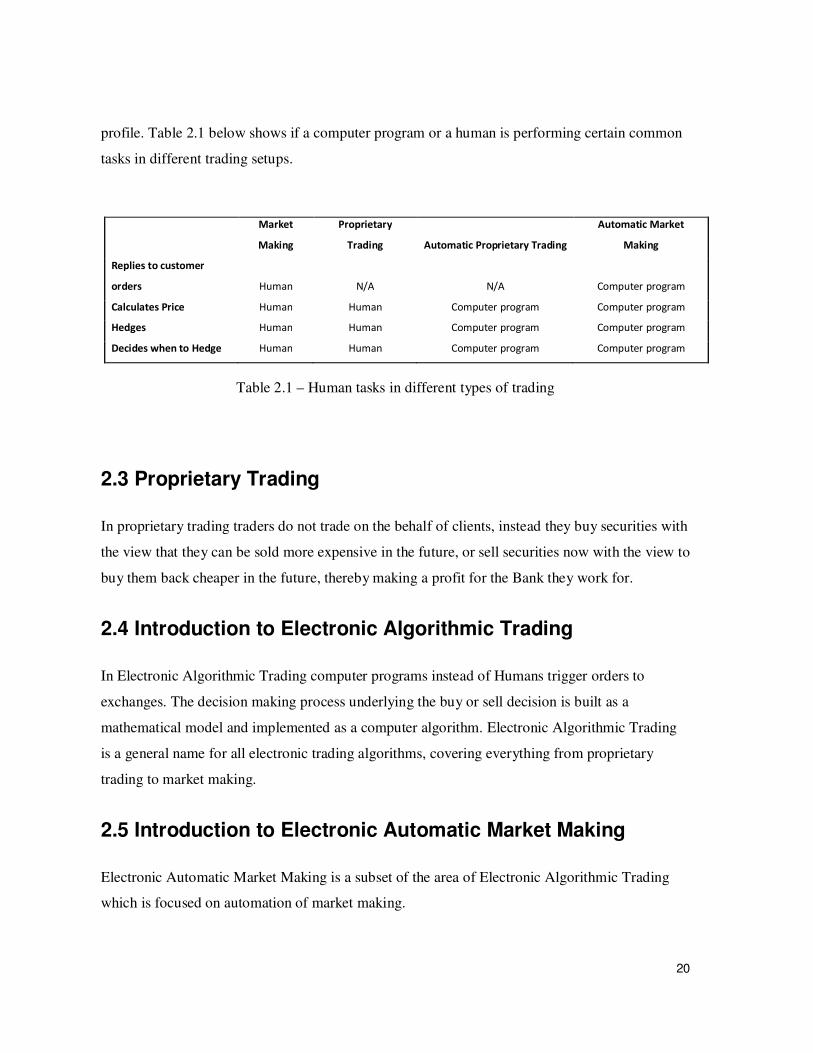
profile. Table 2.1 below shows if a computer program or a human is performing certain common
tasks in different trading setups.
Market
Making
Proprietary
Trading Automatic Proprietary Trading
Automatic Market
Making
Replies to customer
orders Human N/A N/A Computer program
Calculates Price Human Human Computer program Computer program
Hedges Human Human Computer program Computer program
Decides when to Hedge Human Human Computer program Computer program
Table 2.1 – Human tasks in different types of trading
2.3 Proprietary Trading
In proprietary trading traders do not trade on the behalf of clients, instead they buy securities with
the view that they can be sold more expensive in the future, or sell securities now with the view to
buy them back cheaper in the future, thereby making a profit for the Bank they work for.
2.4 Introduction to Electronic Algorithmic Trading
In Electronic Algorithmic Trading computer programs instead of Humans trigger orders to
exchanges. The decision making process underlying the buy or sell decision is built as a
mathematical model and implemented as a computer algorithm. Electronic Algorithmic Trading
is a general name for all electronic trading algorithms, covering everything from proprietary
trading to market making.
2.5 Introduction to Electronic Automatic Market Making
Electronic Automatic Market Making is a subset of the area of Electronic Algorithmic Trading
which is focused on automation of market making.

21
In Electronic Automatic Market Making computer programs instead of Human beings are
responding to client orders. The computer program often also have built in mathematical model,
that gives a view of the market, generating the information required for the program to make the
decision if a position should be hedged away directly, or later.
Another characteristic of Automatic Market Making is that the algorithm tries to hedge away its
position intra-day, meaning that in the ideal case there is no residual overnight position and each
trading day therefore starts from scratch.
2.5.1 Characteristics of a Financial Market suitable for Automatic Trading
In order for a financial market of a certain security type to be suitable for electronic automatic
trading a few conditions have to be fulfilled (Asbridge, 2010):
1. Enough liquidity must be available
2. A highly developed electronic trading capability with firm prices from market
participants
3. A regulatory environment which allows automatic trading.
The first point is important as in order to determine and execute on a fair market price. The
second and the third point is a given prerequisite for any electronic trading.
The Foreign Exchange market fulfills all requirements above and is therefore together with
Equity market in the frontier of this field (Asbrigde I, 2010). This thesis is focused on Automatic
Market Making within the Foreign Exchange market.
2.5.2 Market Participants
The participants in the Automatic Trading field can be split into two types: Sell-side, Buy-side–
participants. Sell-side participants sell investment services to the Buy-side participants.
Typical Sell-side participants are Investment Banks that act as broker-dealers to the Buy-side
participants, e.g. they execute orders on exchanges or with other clients for the Buy-side client.

22
Typical Buy-side participants are Private Equity funds, Hedge Funds, Mutual Funds and
proprietary trading desks.
It´s important to mention that the type of Automatic Market Making that is analyzed in this thesis
is the type done by Banks, and not the type done by Brokers. A broker matches orders from
buyers and sellers and takes therefore no capital at risk. Banks on the other hand first give the
price to the customer and then decide what to do with the residual position. The Bank might
decide to hedge directly, but it might also decide to hedge later. During the time period between
execution of the client order and the hedging, the Bank has a position and therefore faces liquidity
risks. When Banks trade for their own account like this, they are doing Principal Trading.
2.5.3 Competitive Landscape
In order to understand the importance of the investigation done in this thesis it is important to
understand the competitive landscape for the participants in the field of Automatic Market
Making.
In the analysis below the focus is on Automatic Market Making firms, also called automatic
brokers. An analysis using Porters Five Forcers (Porter M.E, 2008) gives the view of the market
presented below. The reason for including this in this thesis is that an automatic market making
system is a significant investment in the hundreds of million dollar range. To make an investment
of this size a corporation needs to understand how big the risk is that new competitors will enter
or how strong the existing rivalry in the industry is.
Threat of New Entrants
In order to participate as an Electronic Market Maker significant investment in IT infrastructure
and Trading Systems are needed. Both buying from a supplier and building in-house will be very
costly.
On top of the IT investments senior specialists in financial mathematics and economics are
needed to build the trading models.
Because of the reasons mentioned above the threat of new entrants is relatively low.

23
Bargaining Power of Suppliers
If the trading firm decided to buy the trading system from a supplier, the supplier power will
increase once the system is in operation as switching costs are both high in money and in time.
If the trading firm decided to build the trading system in-house, suppliers of skilled Software
Engineers will get more bargaining power, as many systems become dependent on a few key
resources who really understands the system.
Because of those reasons the bargaining power of suppliers are medium.
Bargaining Power of Buyers
Some clients can very easily decide to execute their trade with another broker firm if they get a
better price. Some clients choose to developed relatively fixed connections to the automatic
broker firm, because of this their switching cost will be relatively high, nevertheless they don´t
tend to stick around long with a broker that gives them bad prices.
Because of those reasons the bargaining power of buyers are medium to high.
Threat of Substitute Products or Services
There are no real substitutes to brokerage firms that can be used to trade financial securities.
Therefore the threats of substitute products or services are low.
Rivalry among Existing Competitors
There are many Investment Banks competing about being the best in each Automatic Market
Making market. The rivalry among existing competitors is therefore extremely high. In the long
run it’s likely that only a few top firms survive. Figure 2.1 below illustrates the competitive
landscape for a Bank active in Automatic Market Making.

24
Figure 2.1- Competitive Landscape
Conclusions
The main threats are from buyers and suppliers. The threat of substitute products and new
entrants are low. Based on this analysis my conclusion is that Investing in an automatic market
making system is a good and relatively safe investment for corporations that can afford the
upfront investment and have the necessary resources to stay in business until the solution is ready
for production and profitable.

25
2.5.4 Risks
As the electronic market makers investigated in this thesis executes client orders with the aim to
take no position, or at least no overnight position, the key risk is Operational risks (BIS, 2001).
Operational risks can be split into two types, Infrastructure risks and Algorithmic risks.
The most important infrastructure risks are way (Klocker 2010, pers. comm., Feb 2010):
1. Slow connection (high network latency) to market. This makes impossible to execute
trades efficiently.
2. Lost connection to market while holding a large position.
The most important Algorithmic risk is a potential algorithmic malfunction, a so called software
bug. Basically that the algorithmic was implemented in an incorrect way (Klocker 2010, pers.
comm., Feb 2010).
The first risk is an important concern as with a slow connection to the market, the price might
move significantly from the time the order was sent until the order hits the market. To
compensate for this the trading algorithm have to widen the bid ask spread, in order to make sure
the price is still within the order limit when it reaches the exchange. This means a worse price for
the client who means that the client might choose to cancel his relationship with UBS and trade
with another bank that can provide better prices instead.
The second risk, loss of connection to the market, is even more dangerous as it might make
impossible to both execute client orders and hedge positions that are temporarily hold during the
intraday trading. If the outage is for an extended period of time the market prices can move
significantly before the connection is reestablished, possibly resulting in a huge loss. The
immediate problem is to, in a more manual way, get rid or hedge any position that might he held.
This can be done over Hotspots, Cernex, CMI, Reuters, IBS or other electronic exchanges or
interbank communication networks.
Both of the risks above also present a Reputational risk. A bank that often experiences those
problems might lose trust by important clients resulting is a loss of customers (Gillet R et al,
2009).

26
The Market risk faced by a trader depends to a large extent on the trading horizon of the trading
strategy (Klocker 2010, pers. comm., Feb 2010). For long-term strategy with trading horizons of
weeks, months or even years the market risk is the dominant risk. The type of Automatic Market
Making that is investigated in this thesis only takes very short-term intraday positions. This
means that the importance of market risk is very small, instead the availability of liquidity is the
dominant risk.
2.5.5 Information Technology environment
Automatic market making requires state-of-art IT infrastructure and software. A trading firm can
choose between buying the base system of the shelf and only develop the mathematical
algorithms themselves, or develop the entire system in-house. UBS has developed their entire
Foreign Exchange trading system in-house.
Whether buying or building, the basic system components are the same. Figure 2.2 below
illustrates an abstract and simplified view of the basic components of an Automatic Market
Making System.
Figure 2.2 – Components of Automatic Market Making System.
Clients have direct electronic connections into the Main system of the Trading Firm. Client will
send market orders or limit orders into the main system. A market order is an order where client
is happy to get the current market price, a limit order is an order where the client has set a limit on
his orders. For example, a client wants to buy 1 million Swiss Franc and pay with Swedish
27
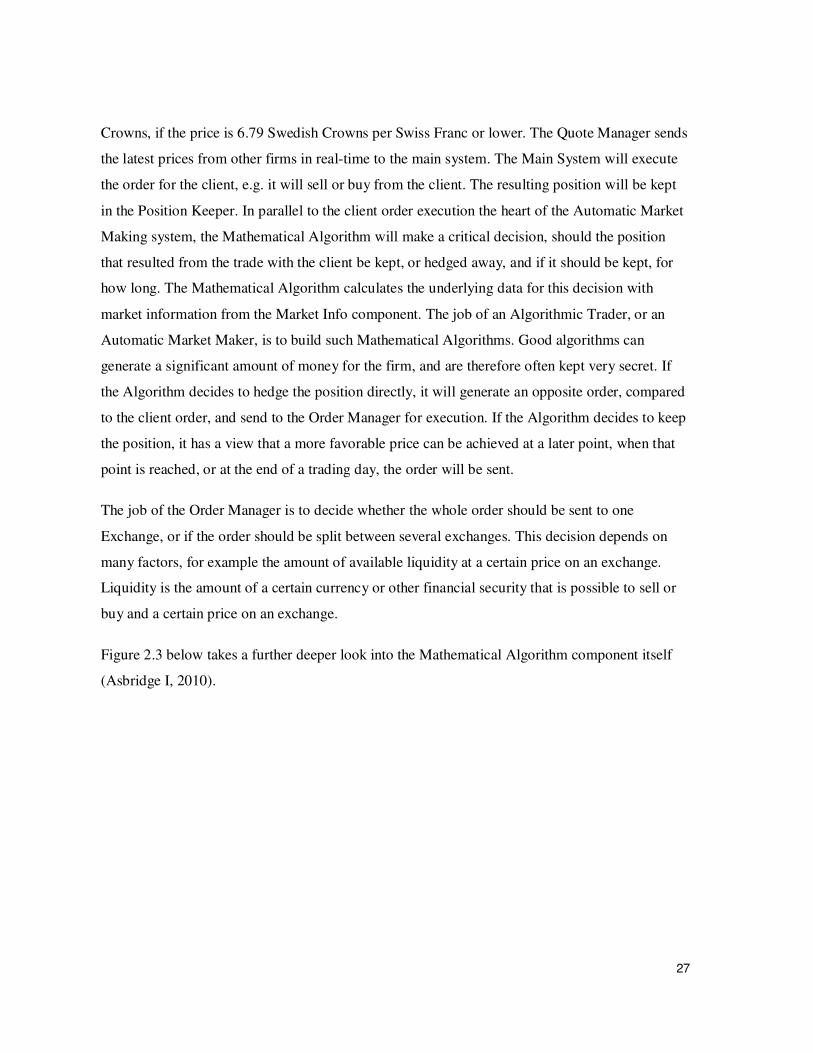
Crowns, if the price is 6.79 Swedish Crowns per Swiss Franc or lower. The Quote Manager sends
the latest prices from other firms in real-time to the main system. The Main System will execute
the order for the client, e.g. it will sell or buy from the client. The resulting position will be kept
in the Position Keeper. In parallel to the client order execution the heart of the Automatic Market
Making system, the Mathematical Algorithm will make a critical decision, should the position
that resulted from the trade with the client be kept, or hedged away, and if it should be kept, for
how long. The Mathematical Algorithm calculates the underlying data for this decision with
market information from the Market Info component. The job of an Algorithmic Trader, or an
Automatic Market Maker, is to build such Mathematical Algorithms. Good algorithms can
generate a significant amount of money for the firm, and are therefore often kept very secret. If
the Algorithm decides to hedge the position directly, it will generate an opposite order, compared
to the client order, and send to the Order Manager for execution. If the Algorithm decides to keep
the position, it has a view that a more favorable price can be achieved at a later point, when that
point is reached, or at the end of a trading day, the order will be sent.
The job of the Order Manager is to decide whether the whole order should be sent to one
Exchange, or if the order should be split between several exchanges. This decision depends on
many factors, for example the amount of available liquidity at a certain price on an exchange.
Liquidity is the amount of a certain currency or other financial security that is possible to sell or
buy and a certain price on an exchange.
Figure 2.3 below takes a further deeper look into the Mathematical Algorithm component itself
(Asbridge I, 2010).

28
Figure 2.3 – Components in an algorithmic trading algorithm
2.5.6 Profit Model
Proprietary trading firms such as Hedge funds earns money by taking a view on the price
development on various financial products with the aim to buy low and sell high or sell high and
buy back low.
Market making desks typically earn money in two ways, by charging a commission for each trade
they perform for a client, and from having a slight price difference between the price they buy for
and the price they sell for. This spread is called Bid-Ask spread. The Bid-Ask spread is calculated
based on both the cost of holding the inventory needed to supply liquidity and the information
disparity between traders (Smithson C.W, 1998). One of the major challenges for the quantitative
analysts who develop the mathematical models behind the Automatic/Algorithmic trading
systems is to define the Bid-Ask spread, and through this do indirect arbitrages (Beunza et al,
2005). The Bid-Ask spread contains many components, for example the view of the future price
development (Payne R, 2003).
Example: The market maker sells one Swiss Franc for 6.80 Swedish Crowns, but he buys one
Swiss Franc for 6.77 Swedish Crowns. If he buys one Swiss Franc from one client for 6.77

29
Swedish Crowns and then tell it to another Client for 6.80 Swedish Crowns, he made a profit of
6.80-6.77 = 0.03 Swedish Crowns.
This thesis is focused on Automatic Foreign Exchange market makers. Because of the high
competition in this industry, they can´t charge commission, they make all their profit on the Bid-
Ask spread (Klocker 2010, pers. comm., Feb 2010). Furthermore Foreign Exchange Spot trading
is a highly commoditized financial product; meaning a high volume, low margin product
(Rockefeller, 2002).
Assuming that the profit distribution for an Automatic market maker follows a normal
distribution the key skill for a trader that writes automatic market making algorithms is to write
algorithms that minimizes the probability of big losses. One big loss might cut a full day of small
profits. Figure 2.4 below illustrates which part of the Bell-shaped profit distribution that should
be avoided by all means possible. (Klocker 2010, pers. comm., May 2010)
Figure 2.4 – Profit distribution
2.6 Summary Chapter 2
This chapter has introduced the Investment Banking industry in general and Automatic Trading in
particular. The participants were introduced and the competitive landscape was explained to show
that even though an investing in a state of the art Automatic Trading system is costly, it is a
relatively safe investment. The different types of trading was explained with particular
empathizes of the IT environment, the risks and the profit model behind Automatic Market
Making.

30
Chapter 3 – Literature review and Model
This chapter will start with a literature review and end in the Model that will serve as the
analytical tool that the research will be based upon.
Several international academic databases where searched, but no relevant paper covering research
that is close enough to the research and modeling done for this thesis where found. The literature
review for the automatic trading area is therefore focused on books. For the investment analysis
part the literature review of academic papers gave better results.
3.1 Literature Review
The importance of Low Network Latency in order for Automatic Trading Systems to produce the
maximal potential revenue is widely known within the Financial Services Industry (Michelsen P
et al, 2009), (Chippas T, 2008). That automatic trading introduces serious operational risks to an
organization and that the Network Latency is one of the most important of those risks are
frequently being discussed (Benyon D, 2010). Discussions on how measurements on Network
Latency can be standardized in the industry are ongoing, until today, no such standard exists
however (Houstoun et al, 2009).
Asbridge I. (2010) has written a comprehensive overview of most aspects that needs
consideration when dealing with any form of Algorithmic Trading, covering everything from the
history of Algorithmic Trading, to different types of Algorithmic trading algorithms and even the
Software Development process of an Algorithmic trading system. Narang R.K. (2009) are
focusing on trading models and trading strategies and Kendall K. (2007) makes a similar general
overview to the one made by Asbridge I. (2010), with a slight stronger focus on order execution
management. King, J.L. (2001) presents tools that can be used when constructing an operational
risk framework and Taleb N.N talks about the impact when highly improbable events really
occur. Grant R.M (2002) talks about market making strategies in general, mainly focused on what
is important for manual market making.
Wagener et al(2010) proves that investment in state of the art trading technology gives improved
price efficiency, which in turns means charging lower fees to customers and therefore increasing

31
market share and overall profit. Chaboud et al (2009) writes that we see a growing market share
from algorithmic/automatic trading in the foreign exchange market. According to Dr. Klocker this
trend lowers the market risk but increases operational and reputational risk. Gillet R et al (2009)
shows that it´s negative for the reputation of a Bank when an operational risk losses is announced
Power (2005) writes that operational risk is rapidly emerging as a key component in global
banking regulation. Smithson C.W, 1998 writes that the larger the information disparity between
the traders, the bigger the Bid-Ask spread needs to be. The longer the latency is, from when a
price update or an order update happens on an exchange until this signal is received in the
Automatic Trading system, the less correct view of prices and order depth the system used for
decision making, which would suggest that Bid-Ask spreads needs to wider, which will force the
Bank to give higher prices to customers, which in turn will mean that less customers will trade
with the Bank and profit will decline. Furthermore Khanna (2009) states that market participants
are continuously driving to reduce latency in order to stay at the top of the competitive trading
landscape.
The articles above supports the statements of Dr Klocker that operational risk is bad for a Banks
reputation and the major risk component in the Foreign Exchange Spot automatic market making.
However, until today, not much research has been done in order to try to investigate exactly how
important Network Latency is for the profitability of an Automatic Market Making System. This
research done in order to write this thesis might be one of the first attempts to address this very
specific problem. As such, this is novel research, and references to similar research are therefore
very limited.
3.2 Model
3.2.1 Introduction to Modeling and Simulation
A model in the general sense is a simplified description of a system, theory or phenomenon that
helps us grasp and understand a part of our complex reality.
We all interpret and manage our daily life through mental models. The reality is however often
too complex to fully understand and our mental models of the reality are therefore often

32
simplified and error prone. On top of this each person has an individual model for every piece of
reality and nobody else can fully understand this model.
Computer modeling is a common way in trying to understand complex systems. A computer
model is a simplified yet explicitly defined view of certain part of the reality that helps us
understand and analyze a particular problem, question, relationship or behavior.
The benefits of a computer model compared to a mental model are (Sterman J.D., 1991):
• A computer model is explicit. All assumptions are stated in a written form and available
for everybody to read.
• They infallibly compute the logical consequences of the modeler´s assumptions.
• They are comprehensive and able to inter relate many factors simultaneously.
In the general sense there are two types of computer models: Optimization Models and Simulation
Models. Optimization models tries to calculate the optimal way of doing a certain thing, for
example, how many calories to eat per day in order to reach a certain target weight in the shortest
possible time. Simulation models try to mimic a real system so that its behavior can be studied
(Sterman J.D., 1991).The model developed in this thesis is a Simulation model.
A Simulation Model must have two parts, a description of the physical world relevant to the
problem under study and a portrait of the behavior of the actors in the system (Sterman J.D.,
1991). In this thesis the physical reality is a simplified automatic market making scenario
described in chapter 3.3 and 3.4. The actors in the system are the market price, the customers and
the profit. The model aims to portrait how they behave within the simplified automatic making
scenario when network latency change.
The obvious benefit with the computer modeling approach is that it makes it possible to in a
relatively cheap and straightforward way simulate the behavior of a complex reality by
simplifying it. The obvious limitation is however that the model will never be better than the
assumptions underlying the model. If these assumptions are bad, the outcome of the model has
little or no value. Sterman J.D. (1991) states that the following areas limit a Simulation model:

33
• The Accuracy of decision rules – The definition of the decision making process of
Actors in the system.
• The choice of Soft Variables – variables that is difficult to measure, such a
Customer Satisfaction or Customer Tolerance to take examples from this Thesis
(Chapter 3.4)
• The Model boundary – Which factors should be included or excluded.
Computer models are frequently used for many different application areas. They are also
frequently discussed, researched and analyzed in the research areas called System dynamics and
Systems thinking (Sterman J.D, 2000).
3.2.2 Philosophy
The philosophy behind the modeling approach was to try to make a clean model that allowed for
a focus on the key research question. The model was designed with the target to strip out other
possible sources of noise that could distort the result. No real units such as milliseconds or dollars
are used in the model. Instead the arbitrary units of profit and latency in used. The goal of the
simulation of this model is find out the relationship between the profitability and the network
latency. Therefore the actual units are not important and would only complicate and distort the
model if introduced.
3.3 Simplified Automatic Market Making Model
The basic business model for the UBS automatic FX spot trading analyzed in this thesis is high
frequency intraday market making. The characteristics of this business model are (Klocker,
2010):
• Large number of trades
• Short position holding periods
• All market risk is directly hedged away by the algorithm.
• Overnight positions are avoided if possible to avoid balance sheet usage and overnight
interested rates costs and large overnight price movements.
• UBS provides a prime brokerage service, where clients can get credit lines in return
for collateral, meaning that they can trade freely within those credit limits.

34
• Most trades are not done over a central clearing house such as an exchange; instead
the trades are cleared directly between banks that trade with each other, regulated
through bi-lateral agreements.
• Typical clients are smaller banks, funds and hedge funds that can´t access the
Electronic Communication Networks needed for FX trading on their own.
• UBS must verify the credit worthiness of the clients before giving credit lines.
• Money is earned on the Bid/Ask spread and efficient hedging. The difference between
the buy and the sell price minus hedging costs.
This thesis will investigate how network latency affects the profit and loss of an Automatic
Market Making Algorithm within the Foreign Exchange spot trading area. The aim will be to
provide a model that predicts how the Profit & Loss is affected when network latency changes.
This would serve as a guide to how much it’s worth investing in redundant IT systems and still
make a profit.
The analysis will start on an abstract version of a real Automatic Trading System and then zoom
in deeper on certain parts of the system. Figure 3.1 below illustrates a simplified view of the
system model covered in chapter 2.5.5.

35
Figure 3.1 - Abstract View of the Automatic Trading System
Figure 3.1 above illustrates the abstract version of the Automatic Trading System. The Algorithm
that does the actual trading is in the blue box. The electronic links to Clients and exchanges are
illustrated with blue arrows. The red box represents the interface to the client who wants to buy or
sell a certain currency, paying in another currency. The green-yellow box illustrates the exchange
where currencies can be bought and sold .
This thesis will not be about building the algorithm itself, instead it will be about analyzing how
different risk events in the surrounding IT system affects how the trading strategy should be built,
and how where it pays investing in IT solutions that minimize the risks for such events to occur,
and where this kind of investment doesn´t pay off, e.g. where manual back-up solution such as a
manual trader is more economically effective to use instead.

36
3.4 Simplified Automatic Market Marking Scenario –
Theoretical Model
The actual model implementation was built based on the following assumptions, creating a
simplified and abstract trading scenario, that focus on the key research question. These
assumptions where formulated together with Dr Thomas Klocker, head of FX Algorithmic
Trading at UBS, and are based on his long experience in Automated Market making in the FX
spot area from Goldman Sachs and UBS. The assumptions are made in order to focus on the core
question which is finding the relationship between profit and network latency.
List of assumptions:
1. Customers buys and sells randomly with equal probability.
This is a realistic assumption for a generic currency pair with no underlying macro
economic trend affecting the flow.
2. Each customer makes an equal amount of trades
This is realistic when focusing on the generic customer.
3. The number of trades per customer is always at least ten times bigger then the number
of customer.
This assumption is made to make the trade variable more important then the customer
variable.
4. The Bid and Ask spread with no network latency is 1 pip. Meaning that Ask is 1 pip
higher than the fair price and Bid is one pip lower than the best price on the market.
Assumption made to simplify the model.
5. There is a limit to how long or short you can get - so once we are long/short a certain
level – the whole position needs to be hedged away before another trade can be done
with a customer, this forces customers to wait, which will make them like the market
maker less.
37
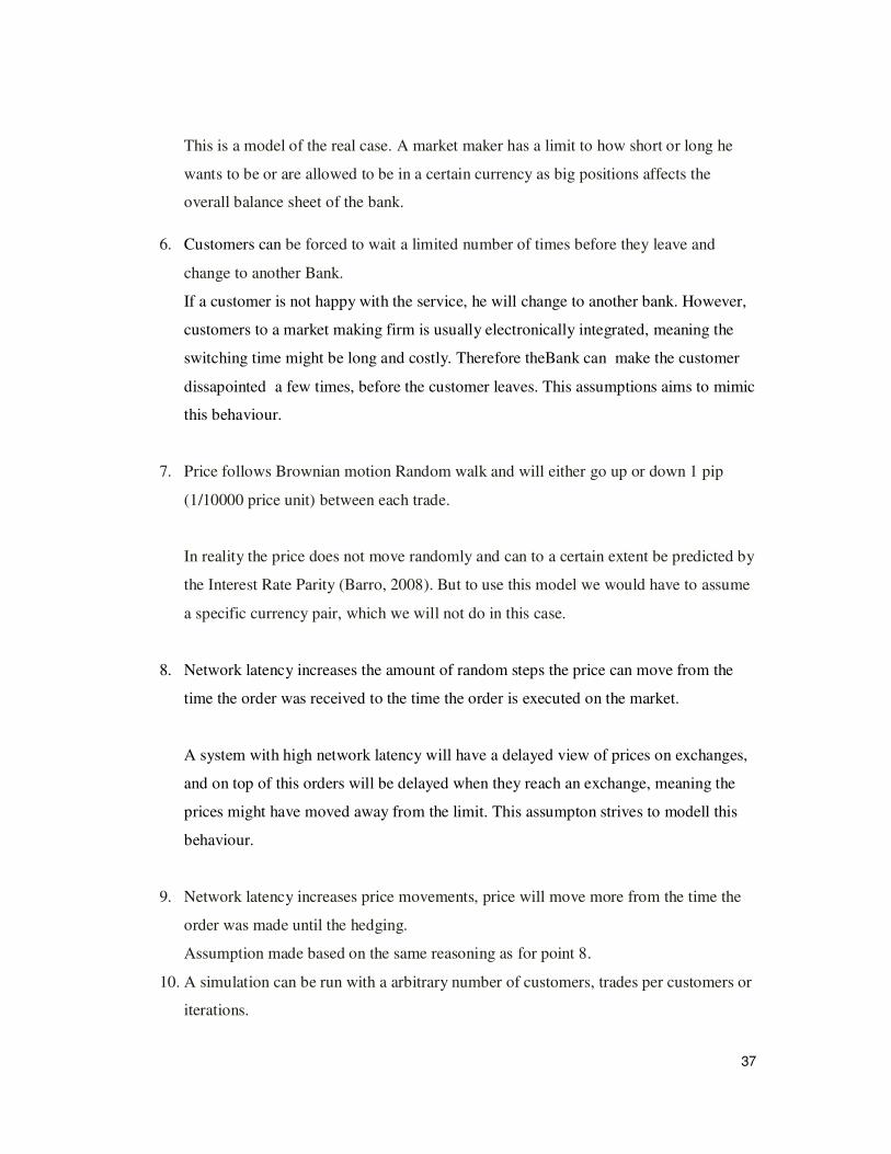
This is a model of the real case. A market maker has a limit to how short or long he
wants to be or are allowed to be in a certain currency as big positions affects the
overall balance sheet of the bank.
6. Customers can be forced to wait a limited number of times before they leave and
change to another Bank.
If a customer is not happy with the service, he will change to another bank. However,
customers to a market making firm is usually electronically integrated, meaning the
switching time might be long and costly. Therefore theBank can make the customer
dissapointed a few times, before the customer leaves. This assumptions aims to mimic
this behaviour.
7. Price follows Brownian motion Random walk and will either go up or down 1 pip
(1/10000 price unit) between each trade.
In reality the price does not move randomly and can to a certain extent be predicted by
the Interest Rate Parity (Barro, 2008). But to use this model we would have to assume
a specific currency pair, which we will not do in this case.
8. Network latency increases the amount of random steps the price can move from the
time the order was received to the time the order is executed on the market.
A system with high network latency will have a delayed view of prices on exchanges,
and on top of this orders will be delayed when they reach an exchange, meaning the
prices might have moved away from the limit. This assumpton strives to modell this
behaviour.
9. Network latency increases price movements, price will move more from the time the
order was made until the hedging.
Assumption made based on the same reasoning as for point 8.
10. A simulation can be run with a arbitrary number of customers, trades per customers or
iterations.

38
This assumption was made to be able to taste any size of trading scenario.
11. A clock - each step decided if price go down/up and if there is a trade - can be trade
and price move, or only one of them
A natural way to implement this modell into a software application.
The results generated from the simulation runs of the model will be compared to the case
of the ideal market maker that experiences no network latency and the maximum number
of customers possible.
3.5 Advanced Extensions to Basic model
In the second part of the research work the model was extended with three more advanced
concepts under the assumption that this will make the model more realistic. Those assumptions
are also based on interviews with Dr. Thomas Klocker, Head of FX Algorithmic Trading at UBS.
1. Highly improbable big price jumps where introduced. This occurs in the real foreign
exchange market and can be seen as a Black Swan effect (Taleb , N.N 2007) and can be
used sudden price jumps that represent big economic events, such as interventions from
governments.
2. A Price Trend was introduced. This means that for each random step the price takes, there
is a slightly higher probability that the price will move in the direction of the trend, then in
the other direction. This trend will change at regular interval and the Bank will either
know about the trend or not. This assumption aims to simulate macro economic trends
which affect exchange rates. (Dornbusch, 1989).
3. Variable Hedge Costs that increases with Network latency was introduced. This aims to
modell the fact that higher latency requires wider Bid/Ask spreads when hedging, which
means higher hedging costs. In the same way, lower latency means more effective pricing,
tighter Bid/Ask spreads and therefore lower hedging costs. Wagener Et al (2010).

39
3.6 Summary Chapter 3
This chapter has covered the literature review and the developed of the basic model that will be
implemented in the simulator. It also covered the advanced extension made in the later part of the
thesis work.

40
Chapter 4- Model implementation and
simulation
This chapter will build upon on the theoretical ideas in Chapter 3 develop and algorithm and a
simulator. Furthermore simulations will be run and the results will be presented.
4.1 Components in Model
The model will contain the following parts:
• An Algorithm that defines the random walk of the price with and without network
latency.
• An algorithm that determines whether the price should move or a trade should be done
at each clock tick.
• A trading model and a execution model that runs the trades and determines if the
automatic market maker can hedge directly, or if hedging should be done later. The
trading model will also determine when the maximum long limit and the maximum
short limit is reached, forcing a full hedge to flatten position.
• An algorithm model that calculates profit and loss for the simulation run.
• An algorithm that calculates how customers decrease when they are forced to wait.
• A Windows based user interface that allows the user to set simulation parameters and
start/stop the simulation. Output will be profit and number of customers left.
The outcome of the simulation will be how many percent of the ideal market makers profit and
loss that is achieved with a certain level of network latency. This data can then be used to
calculate how large in percentage of the profit and loss and IT investment with a lifetime of three
years can be in order to still generate a decent profit assuming a certain cost of capital for UBS
for investing in the Automatic Market Making system.

41
4.2 Implementation
4.2.1 Programming Language
The model was implemented as a Windows application using the Microsoft .NET C#
programming language using Microsoft Visual C # 2008 Express Edition which is a free rich
integrated development environment provided by Microsoft.
4.2.2 Algorithm – Flow Diagram and explanation of Algorithm
Figure 4.1 below illustrates a flow diagram of the current implementation of the Algorithm basic
algorithm. Each step is numbered and described with text below the flow diagram.
The advanced extensions described in chapter 3.5 is not part of the algorithm description and the
flow diagram below, instead they are described separately in chapter 4.2.3.

42
Figure 4.1 - Flow diagriam of Algorithm implementation

43
Description of Steps in Algorithm
Each step in the algorithm its described here, the C# source code can be found in Appendix A.
1. Number of clock ticks calculated. Nr of ticks = nr of customers * nr of trades per customer * 2.
The factor 2 is needed as 50% of the ticks will be trades and 50% will be price moves.
2. The algorithm runs a loop, this check determines when the simulation run is finished, e.g. if
total number of ticks run are equal to total number of ticks that should be run.
3. This step determines if the current clock tick should result in a price move or a customer
order/trade.
4. Price Move. The price Class will move the price.
5. Get current market price.
6. This step determines if the customer wants to Buy, otherwise the customer wants to Sell.
7. Here we check how short we already are. If we are shorter then the maximum short limit, we
have to hedge away all positions before selling to the customer.
8. If we had reached the maximum short limit, we put the customer order execution on hold until
we have hedged away our current short positions. This is bad for our reputation, we increase
customer reputation hits with 1.
9. Get the current market price
10. Hedge all current short positions by buying back to market price to get a flat position. Set
short counter to 0.
11. Calculate profit. A negative profit means a Loss. The profit is the difference between the price
we earlier sold to the client at and the price we buy back at the market for.
12. Now when we have hedged away our short positions, we can sell again to the customer.

44
13. Get Bank price. The bank price is affected by network latency. The higher the network
latency, the more random steps the price can take, before the Bank order reaches the exchange.
14. If Bank price is smaller or equal to the Client price then we hedge directly, otherwise we
hedge later.
15. Hedge directly by selling to the client and buying at the exchange.
16. Calculate profit
17. Bank price was not smaller or equal to the client price. Sell to Client, but keep position.
18. Increase short counter.
19. Here we check how long we already are. If we are longer then the maximum long limit, we
have to hedge away all positions before buying from the customer.
20. If we had reached the maximum long limit, we put the customer order execution on hold until
we have hedged away our current long positions. This is bad for our reputation, we increase
customer reputation hits with 1.
21. Get the current market price
22. Hedge all current long positions by selling to market price to get a flat position. Set long
counter to 0.
23. Calculate profit. A negative profit means a Loss. The profit is the difference between the price
we earlier bought from the client at and the price we sell back at the market at.
24. Now when we have hedged away our short positions, we can buy from the customer.
25. Get Bank price. The bank price is affected by network latency. The higher the network
latency, the more random steps the price can take, before the Bank order reaches the exchange.
26. If Bank price is greater or equal to the Client price then we hedge directly, otherwise we
hedge later.

45
27. Hedge directly buy buying from the client and selling at the exchange.
28. Calculate profit
29. Bank price was not higher or equal to the client price. Buy from Client, but keep position.
30. Increase Long counter.
31. If the customer has got as many hits as its defined tolerance, we loose one customer.
32. Decrease customer count.
33. To see the effects of losing one customer, we decrease the number of clock ticks in the
simulation run with number of {trades per customer} * 2 – e.g. we lose all trades for that
customer.
4.2.3 Description of Advanced Extensions
Improbable Big price moves
If big price moves are enabled in the model, the price will make a big jump of a random size with
a certain probability each time the price ticks. The model takes two parameters to determine this.
One parameter sets the probability that a big move will happen. This parameter is integer value
from 0 to 100. A value of 0 means that the big move always happens and a value of 100 means
that the jump will occur once per 100 price ticks.
The size of the jump is determined by another input parameter to the model. If the model
determines that a price jump will occur, the move will be 5 pips plus a random number from 0 to
an integer value determined by the second input parameter to the model.
46
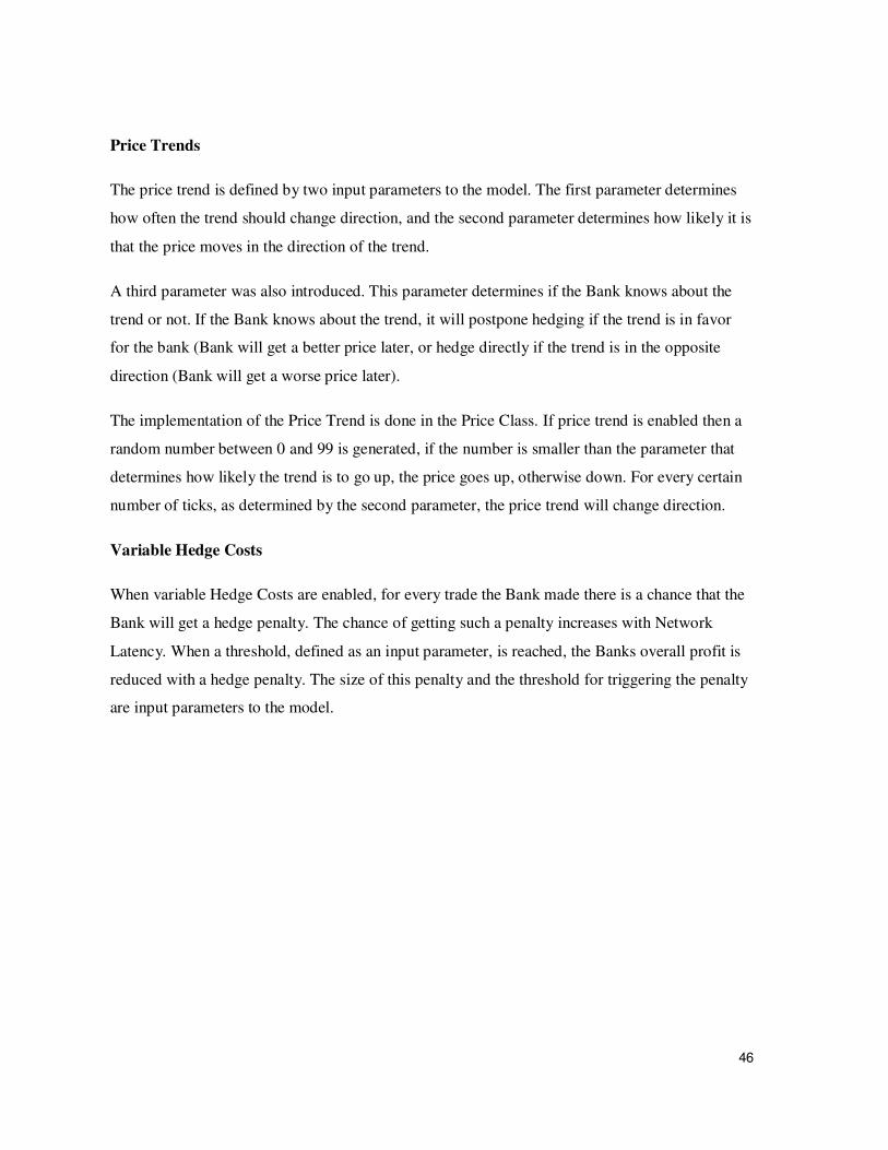
Price Trends
The price trend is defined by two input parameters to the model. The first parameter determines
how often the trend should change direction, and the second parameter determines how likely it is
that the price moves in the direction of the trend.
A third parameter was also introduced. This parameter determines if the Bank knows about the
trend or not. If the Bank knows about the trend, it will postpone hedging if the trend is in favor
for the bank (Bank will get a better price later, or hedge directly if the trend is in the opposite
direction (Bank will get a worse price later).
The implementation of the Price Trend is done in the Price Class. If price trend is enabled then a
random number between 0 and 99 is generated, if the number is smaller than the parameter that
determines how likely the trend is to go up, the price goes up, otherwise down. For every certain
number of ticks, as determined by the second parameter, the price trend will change direction.
Variable Hedge Costs
When variable Hedge Costs are enabled, for every trade the Bank made there is a chance that the
Bank will get a hedge penalty. The chance of getting such a penalty increases with Network
Latency. When a threshold, defined as an input parameter, is reached, the Banks overall profit is
reduced with a hedge penalty. The size of this penalty and the threshold for triggering the penalty
are input parameters to the model.

47
4.3 User Interface
Figure 4.3 – User Interface of Simulator
Figure 4.3 above is a screenshot of the simulation tool. The user can enter the following
parameters to the simulation.
Long/Short Limit: The maximum short or long position the Bank is allowed to have.
Customers: Number of customers at start
Trades: Number of trades per customer.
Network delay: Number of price moves between order entry and trade execution. Default value
of 0 means no network delay.

48
Iterations: This value determines how many times the simulation should be run before the result
is printed. When this value is higher than one, the average result is calculated. This is a useful
feature to get rid of noise by averaging it away.
Customer tolerance: How many times a customer can be forced to wait for the market maker
when he is hedging out a full long or short position, or get a bad price, before leaving the Bank.
Enable big price moves: Determines if Big Price moves should be included in the simulation or
not.
Period: Determines how likely it is that a big price move will occur. The default
value of 100 means a big jump occurs every 100 times the price moves.
Size: Determines how big the Price Jump will be if it happens. The default value
of 6 means the size of the Jump is 5 to 10, e.g. 5 + a random number from 0 to 5.
Enable price trend: Determines if the Price Trend should be used or not.
Trend Period: Determines how many clock ticks the price will keep the same
direction. The default value of 100 means that the price change direction every 100 price moves,
which is every 200 clock ticks.
Percentage Up: Determines how strong the price trend is. The default value of
60 means that there is a 60% chance that the price moves up when the direction is up, and a 60%
chance that the price moves down when the direction is downward sloping.
Bank knows trend: Determines if the Bank knows the trend or not.
Enable Variable Hedge Cost: Determines if the Hedge penalty subsystem should be turned on
or not.
Penalty size: How many points should the Banks profit be reduced with if the penalty is
triggered.
Penalty Trigger: Determines how many Hedge penalties the Bank can get, before the profit
is reduced by the Penalty size.

49
4.4 Simulations with Basic model
Three simulations were run with the model described in chapter 3.4 to simulate how profitability
varies with increased network latency at different levels of customer tolerance. Each simulation
varied the network latency parameter from 0 to 10. Three different levels of the customer
tolerance value were used. The first simulation used a customer tolerance of 5, meaning that the
customer can be forced to wait up to 5 times, once the customer is forced to wait 6 times, that
customer is lost. This value was set to 10 in simulation 2 and to 20 in simulation 3. 20 iterations
were run for each network latency level in each simulation, output variables per network latency
levels were:
• Average Profit
• Average Profit per Trade
• Average Number of Customer Left
• Average end market price.
Table 4.1below contains the detailed settings for each simulation.
Simulation 1 Simulation 2 Simulation 3
Customers 100 100 100
Trades per
customer 1000 1000 1000
Model Iterations 20 20 20
Customer
tolerance 5 10 20
Total Model runs 200000 200000 200000
Start Market price 10000 10000 10000
Max/Long position 10 10 10
Table 4.1 – Settings for Simulation 1, 2 and 3
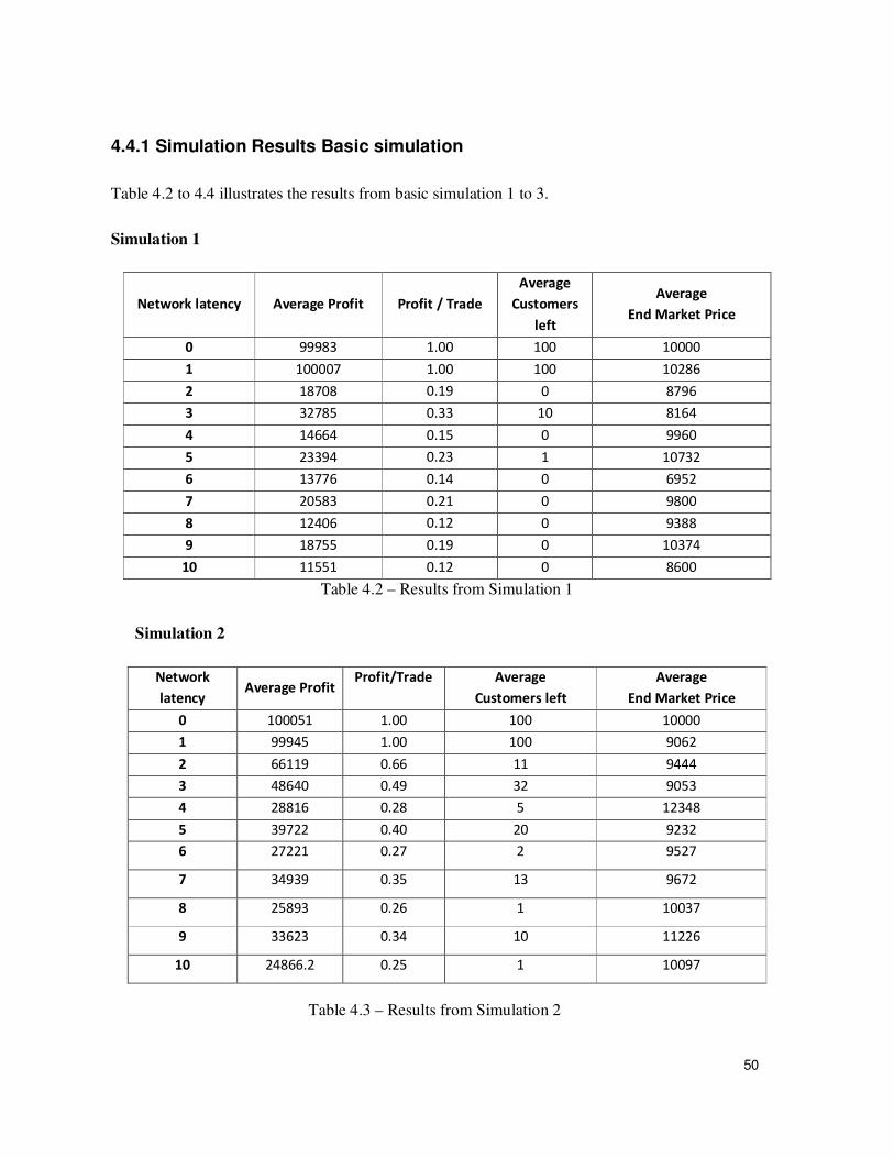
50
4.4.1 Simulation Results Basic simulation
Table 4.2 to 4.4 illustrates the results from basic simulation 1 to 3.
Simulation 1
Network latency Average Profit Profit / Trade
Average
Customers
left
Average
End Market Price
0 99983 1.00 100 10000
1 100007 1.00 100 10286
2 18708 0.19 0 8796
3 32785 0.33 10 8164
4 14664 0.15 0 9960
5 23394 0.23 1 10732
6 13776 0.14 0 6952
7 20583 0.21 0 9800
8 12406 0.12 0 9388
9 18755 0.19 0 10374
10 11551 0.12 0 8600
Table 4.2 – Results from Simulation 1
Simulation 2
Network
latency Average Profit
Profit/Trade Average
Customers left
Average
End Market Price
0 100051 1.00 100 10000
1 99945 1.00 100 9062
2 66119 0.66 11 9444
3 48640 0.49 32 9053
4 28816 0.28 5 12348
5 39722 0.40 20 9232
6 27221 0.27 2 9527
7 34939 0.35 13 9672
8 25893 0.26 1 10037
9 33623 0.34 10 11226
10 24866.2 0.25 1 10097
Table 4.3 – Results from Simulation 2
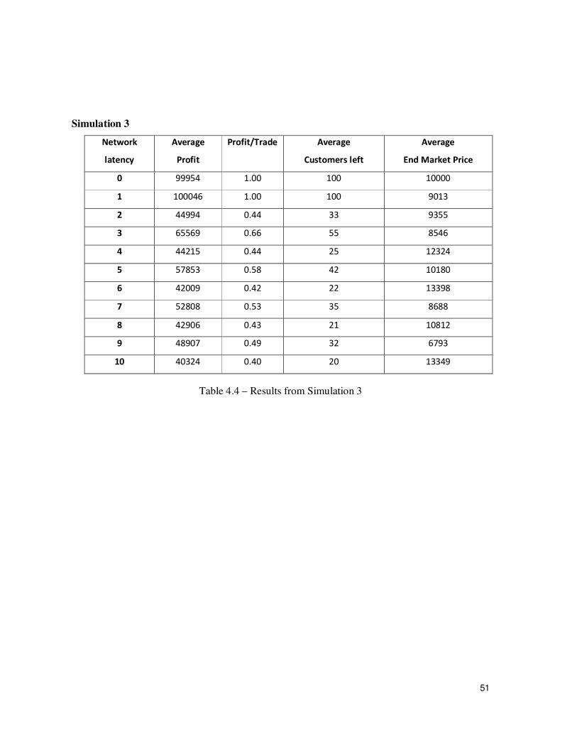
51
Simulation 3
Network
latency
Average
Profit
Profit/Trade Average
Customers left
Average
End Market Price
0 99954 1.00 100 10000
1 100046 1.00 100 9013
2 44994 0.44 33 9355
3 65569 0.66 55 8546
4 44215 0.44 25 12324
5 57853 0.58 42 10180
6 42009 0.42 22 13398
7 52808 0.53 35 8688
8 42906 0.43 21 10812
9 48907 0.49 32 6793
10 40324 0.40 20 13349
Table 4.4 – Results from Simulation 3

52
4.5 Simulations with Advanced Model
The improved model with extensions has a large number of variable inputs that can be varied. In
order to be able to fit this work into the framework of this Thesis the default settings for the new
model extensions constant were kept constant. In order to isolate the effect of each model
extension the benchmark run from the basic model as was used as a reference, Simulation 3, then
one run per new advanced feature was done, plus an additional two with all three new features
turned on. Table 4.5 illustrates the input settings for the simulations with the advanced model.
Default settings:
Big Price Jumps: Period 100, Size 6
Price Trend: Percentage up 60, Trend Period 100
Variable Hedge Cost: Penalty Size 1, Penalty Trigger, 10
Simulation # Reference 1 2 3 4 5 6
Customers 100 100 100 100 100 100 100
Trades per customer 1000 1000 1000 1000 1000 1000 1000
Model Iterations 20 20 20 20 20 20 20
Customer tolerance 20 20 20 20 20 20 20
Total Model runs 200000 200000 200000 200000 200000 200000 200000
Start Market price 10000 10000 10000 10000 10000 10000 10000
Max/Long position 10 10 10 10 10 10 10
Big Price Jumps Off On Off Off Off On On
Price Trend Off Off On On Off On On
Bank knows Trend Off Off On Off Off On Off
Variable Hedge Cost Off Off Off Off On On On
Table 4.5 – Settings for advanced simulation

53
4.5.1 Simulation Results - Advanced Simulation
The results from the reference simulation can be seen in table 4.4. Table 4.6 to 4.11 below
illustrates the results from the advanced simulations.
Network
latency
Average
Profit
Profit /
Trade
Average
Customers
left
Average
End Market Price
0 99988 1.00 100 10000
2 92783 1.00 90 10066
4 85939 0.99 82 13403
6 81168 1.00 75 8767
8 73170 0.95 69 8258
10 73395 1.01 64 11066
Table 4.6 – Results, Advanced simulation 1, Price Jumps
Network
latency
Average
Profit
Profit /
Trade
Average
Customers
left
Average
End Market Price
0 28767 1.00 28 10000
2 93113 2.70 13 10420
4 108358 3.13 12 9286
6 101210 2.96 12 12159
8 79894 2.36 13 11814
10 58478 1.70 12 13636
Table 4.7 – Results, Advanced simulation 2- Trend, Bank knows trend

54
Network
latency
Average
Profit
Profit /
Trade
Average
Customers
left
Average
End Market Price
0 99923 1.00 100 10000
2 32095 0.66 31 9874
4 43040 0.28 24 10161
6 11600 0.29 22 9319
8 22140 0.56 19 6926
10 37088 0.95 17 9562
Table 4.8 – Results, Advanced simulation 3- Trend, Bank does not know
Network
latency
Average
Profit
Profit /
Trade
Average
Customers
left
Average
End Market Price
0 100021 1.00 100 10000
2 48053 0.96 32 10541
4 41536 0.94 26 10058
6 38499 0.92 23 13715
8 37906 0.92 21 11554
10 36600 0.92 20 10629
Table 4.9 – Results, Advanced simulation 4- Variable Hedge Costs
Network
latency
Average
Profit
Profit /
Trade
Average
Customers
left
Average
End Market Price
0 28763 1.00 28 10000
2 52746 1.53 13 8195
4 56625 1.65 12 8916
6 54275 1.59 12 13359
8 46615 1.37 12 8870
10 38792 1.14 12 11800
Table 4.10 – Results, Advanced simulation 5 – All combined, Bank knows trend

55
Network
latency
Average
Profit
Profit /
Trade
Average
Customers
left
Average
End Market Price
0 100007 1.00 100 10000
2 88403 0.95 90 9536
4 79115 0.92 82 8025
6 74831 0.92 75 13020
8 72167 0.94 69 6679
10 66958 0.92 64 10796
Table 4.11 – Results, Advanced simulation 6 – All, Bank does not know trend
4.6 Summary Chapter 4
This chapter has showed how the theoretical model presented in Chapter 3 was implemented as
an algorithm and how a simulator was done to run this model. The results from the simulations
were also presented.

56
Chapter 5 – Discussion and Conclusions
This chapter will present the simulation results in graphical format and the results will be
analyzed and discussed, culminating in conclusions. Furthermore the results from the simulation
will be put in context of a business case where senior management want to decide how much to
invest in an Automatic Electronic Market Making System.
5.1 Analysis – Basic model
5.1.1 Profit versus Network latency
Figure 5.1 below illustrates how profit varies with network levels for the three Customer
Tolerance (CT) levels used in the simulations.
Figure 5.1 – Profit versus Network Latency
0
20000
40000
60000
80000
100000
120000
0 1 2 3 4 5 6 7 8 9 10
P
r
o
f
i
t
Network Latency
Profit versus Network Latency
Average Profit (CT=5)
Average Profit (CT =10)
Average Profit (CT=20)

57
Simulations results clearly show that profits decline with network latency. When network latency
is set to 2, meaning that the price can make two random steps before the Bank price is given a
sharp drop in profitability, after that it can clearly be seen that profitability drops with higher
network latency for all customer tolerance levels. The overall profit is to a large extend depending
on customer retention, and as can be seen when comparing the graph from the simulation with the
highest customer tolerance (green line) with the graph from the simulation with the lowest
customer tolerance (blue line) the model shows more resistance to network latency with higher
customer tolerance.
5.1.2 Customers left versus network Latency
Figure 5.2 below illustrates how many customers the Bank has left after at different levels of
network latency, for the three Customer Tolerance levels simulated.
Figure 5.2 – Customers left versus Network Latency
0
20
40
60
80
100
120
0 1 2 3 4 5 6 7 8 9 10
Cu
sto
me
rs l
eft
Network latency
Customers left versus Network Latency
Customers left (CT=5)
Customers left (CT=10)
Customers left (CT=20)
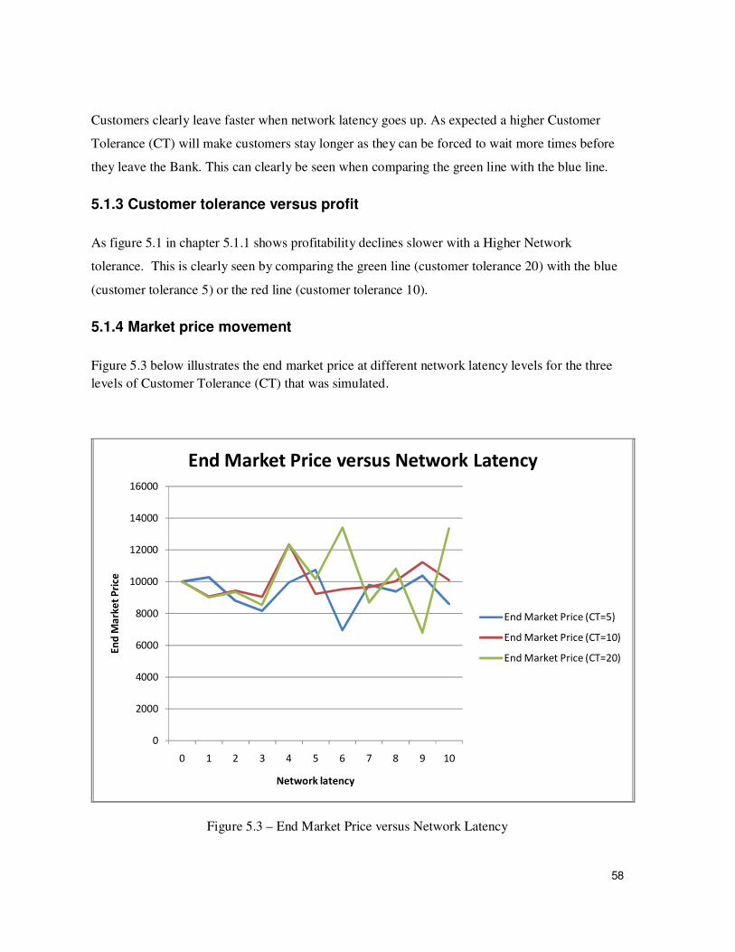
58
Customers clearly leave faster when network latency goes up. As expected a higher Customer
Tolerance (CT) will make customers stay longer as they can be forced to wait more times before
they leave the Bank. This can clearly be seen when comparing the green line with the blue line.
5.1.3 Customer tolerance versus profit
As figure 5.1 in chapter 5.1.1 shows profitability declines slower with a Higher Network
tolerance. This is clearly seen by comparing the green line (customer tolerance 20) with the blue
(customer tolerance 5) or the red line (customer tolerance 10).
5.1.4 Market price movement
Figure 5.3 below illustrates the end market price at different network latency levels for the three
levels of Customer Tolerance (CT) that was simulated.
Figure 5.3 – End Market Price versus Network Latency
0
2000
4000
6000
8000
10000
12000
14000
16000
0 1 2 3 4 5 6 7 8 9 10
En
d M
ark
et
Pri
ce
Network latency
End Market Price versus Network Latency
End Market Price (CT=5)
End Market Price (CT=10)
End Market Price (CT=20)

59
As illustrated in figure 5.3 the price has moved in a completely random manner as expected as the
market price movement is implemented as a random walk. It can also be seen that the amplitude
of the price movements increase with network latency, this is also expected as for each level of
network latency the price makes one random step.
5.2 Analysis – Advanced model with extensions
This section analysis the new model extensions in comparison with the basic model reference
case.
5.2.1 Big Price Jumps
Figure 5.4 – Model with Price Jumps enabled
Figure 5.4 above shows that when big price jumps is enabled the profit declines slower then when
it´s not turned on. This can be explained as the Bank manages to retain more customers when
there are random price jumps, meaning more trades will be done. This can be seen in the result
tables in Chapter 4. Comparing the red line with the blue line clearly shows that profitability of
the model shows more resistance to network latency when random price jumps are enabled.
0
20000
40000
60000
80000
100000
120000
0 2 4 6 8 10
Pro
fit
Network Latency
Big Price Jumps
Reference Case
Price Jumps Enabled

60
5.2.2 Price Trend
Figure 5.5 – Model with Price Trend Enabled
Figure 5.6 – Model with Price Trend Enabled, Profit per Trade
0
20000
40000
60000
80000
100000
120000
0 2 4 6 8 10
Pro
fit
Network Latency
Price Trend
Refence Case
Trend, Bank knows
Trend, Bank does not know
0.00
0.50
1.00
1.50
2.00
2.50
3.00
3.50
0 2 4 6 8 10
Pro
fit
pe
r T
rad
e
Network Latency
Profit per Trade
Reference Case
Trend, Bank knows
Trend, Bank does not know
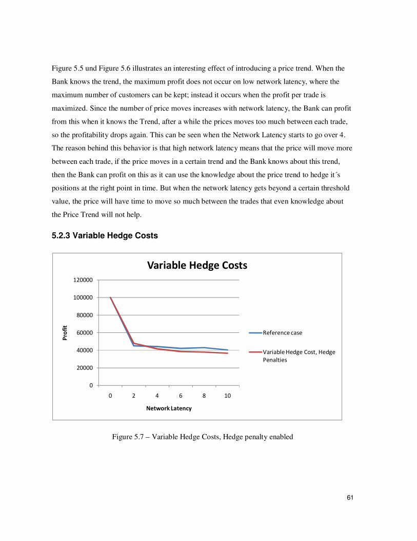
61
Figure 5.5 und Figure 5.6 illustrates an interesting effect of introducing a price trend. When the
Bank knows the trend, the maximum profit does not occur on low network latency, where the
maximum number of customers can be kept; instead it occurs when the profit per trade is
maximized. Since the number of price moves increases with network latency, the Bank can profit
from this when it knows the Trend, after a while the prices moves too much between each trade,
so the profitability drops again. This can be seen when the Network Latency starts to go over 4.
The reason behind this behavior is that high network latency means that the price will move more
between each trade, if the price moves in a certain trend and the Bank knows about this trend,
then the Bank can profit on this as it can use the knowledge about the price trend to hedge it´s
positions at the right point in time. But when the network latency gets beyond a certain threshold
value, the price will have time to move so much between the trades that even knowledge about
the Price Trend will not help.
5.2.3 Variable Hedge Costs
Figure 5.7 – Variable Hedge Costs, Hedge penalty enabled
0
20000
40000
60000
80000
100000
120000
0 2 4 6 8 10
Pro
fit
Network Latency
Variable Hedge Costs
Reference case
Variable Hedge Cost, Hedge
Penalties

62
As expected the profits will be slightly lower when the hedge costs increases with network
latency. Figure 5.7 above illustrates this. This affects can see by comparing the red line (hedge
penalties enabled) with the blue line (no hedge penalties).
5.2.4 All advanced features turned on
Figure 5.8 – All Advanced Features Enabled
From Figure 5.8 it can be seen that the model with all advanced features turned on clearly shows
a great resistance to network latency when the Bank does not know about the Trend. When the
Bank knows about the trend, it will first earn more money than the reference case when the
network latency is a bit higher, this is because of the extra price moves that then occurs, which
the Bank can profit from knowing the trend.
0
20000
40000
60000
80000
100000
120000
0 2 4 6 8 10
Pro
fit
Network Latency
All Advanced Features Enabled
Reference Case
All On, Bank knows Trend
All On, Bank does not know
Trend

63
5.2.5 Profit per Trade, All cases
Figure 5.9 – Profit per trade with different parts of the model turned on
Figure 5.9 shows how the profit per trade varies with network latency when different cases in the
model are turned on. It can clearly be seen that each new extension alters the profit per trade
curve compared to the reference case. Most effect comes from using a price trend and let the bank
know about it. That the Bank knows about the price trend is true to a certain extent, as a big
Investment Bank like UBS can see the flow of orders coming from Client, and use this
information to predict the price movement on the short horizon, based on the current order flow
and the pending order stack.
5.3 Discussion
5.3.1 Impact of network latency on profitability based on Basic model
Figure 5.1 in chapter 5.1.1 shows a sharp decline in profits when network latency goes up. Most
of the profits are lost when network latency increases a bit over the optimum performance of 0,
Figure 5.10 below shows a zoomed in version of figure 5.1.
0.00
0.50
1.00
1.50
2.00
2.50
3.00
3.50
0 2 4 6 8 10
Pro
fit
Pe
r T
rad
e
Network Latency
Profit Per Trade, All cases
Price Jumps
Trend, Bank knows
Trend, Bank does not know
Variable Hedging Costs
All On, Bank Knows Trend
All On, Bank does not know
Trend
Reference Case

64
Figure 5.10 – Zoomed in Profit versus Network Latency, Basic model
When network latency goes from 1 to 2 profits drop sharp for all levels of network latency.
The conclusion from those results are; that a Bank should either invest to have the fastest possible
network connection to the exchange, or stick to average network performance, there is no clear
benefits in investing money to get the second best network on the market.
However, when turning on the advanced features, it can be observed that the Bank could
maximize its profits per trade, if the Bank can develop models that predict the price development
in the market. However, this leads to more lust customers with the current model, as the
long/short limit is reached more often when the Bank choose to hedge later frequently. Because
of this secondary effect the profit is maximized when there is a Trend, and the Bank does know
about it even with a fair portion of network latency. This can be seen in the green line in Figure
5.8. However, more research would have to be done to confirm this hypothesis.

65
5.3.2 Impact of network latency on Customer retention based on Basic
model
As stated earlier in this thesis reputational risk is one of the key operational risks a Bank dealing
with Automatic Market Making, faces. As showed chapter 5.1.2 the Bank quickly loose
customers when network latency goes up. When customers disappear business is lost and
profitability goes down. As the tables in chapter 4.5.1 shows it clearly very important to have the
lowest possible network latency. The simulations show the largest proportion of the customer is
lost when network latency goes from 1 to 2 on all customer tolerance levels. With Customer
Tolerance set to 5, all customers are lost when network latency goes to 2. At a Customer
Tolerance level of 10, 89% of the customers are lost at network latency 2, and with a Customer
Tolerance of 20, 77% of the customers are lost at network latency of 2.
My conclusion here is the same as in chapter 5.3.1, a Bank should either invest to have the fastest
possible network connection to the exchange, or stick to average network performance, there is
no clear benefits in investing money to get the second best network on the market.
5.4 Investment Analysis
Having a state of the art Automatic Market making system with a minimal latency is not an end,
but a means to an end. The final goal is to improve the overall profitability of the Bank running
the system. This section will analyze if investing in an upgrade of an existing Automatic Market
System with average performance to top performance, with respect to Network Latency, gives an
acceptable return on Investment.
First some light will on how big the turnover and the profits in the Foreign Exchange Spot trading
business are. Second the underlying assumptions which the investment analysis is based on will
be presented, last the investment analysis will be done and the results analyzed.

66
5.4.1 Economic Background
According to the Euromoney FX Survey 2010 the total volume of the Foreign Exchange Spot
Trading Market is 87114 billion USD per year. UBS has a market share of 8.22% which
translates to around 7160 billion USD per year. UBS will automate the market making of 85-95%
of this trading (Magnusson 2010, pers. Comm., Sep 2010). This means that a transaction volume
ranging from 6086 to 6803 billion USD will flow through UBS´s Automatic Foreign Exchange
Spot Market Making Systems. Unfortunately the profit margin is a company secret (Magnusson
2010, pers. Comm., Sep 2010), but assuming a profit margin of 0.25% this would translate to a
yearly profit of between 15 and 17 billion USD from the Automated FX market making system.
5.4.2 Background to Investment Analysis
A proper valuation of an IT investment is difficult as there are both direct and indirect benefits,
and some are more tangible then others. A direct tangible benefit from an Automatic Market
Making System with lower Network Latency is the assumed increased profit. An indirect benefit
is for example improved reputation among customers which might lead to increased profits in
another business division of UBS.
There are many methods that can be used to assess the true value of an IT investment. One of
them is the PENG model (Dahlgren et al, 2006). Using the PENG model the benefits and costs
are separated into different categories:
Benefits: Direct benefits, indirect benefits and intangible benefits.
Costs: Costs for achieving the benefits.
Using this model the befits and costs for upgrading a average Automatic FX spot Market Making
System to a state of the art system could look like this:
Costs
- Development cost of new software, meaning salaries to software developers, managers and
financial analysts involved in the system development.
- Cost of new computer and network hardware

67
- License costs for new software components bought from a third party supplier.
- Maintenance costs to keep the system running over its expected lifetime.
Direct Benefits
- Increased revenue from FX market making operation.
Indirect Benefits
- Increased revenue in other business divisions.
Intangible Benefits
- Better reputation among customers, which is likely to lead to even more profitable business in
the future.
Assumptions
During this research the following assumptions where made:
1) Maintenance costs for the upgraded system are the same, or close to the same, as for the
original system.
2) Hardware and license costs for the upgraded system are the same, or close to the same, as for
the original system.
3) The direct, indirect and intangible benefits are all built in to the simulation model.
With these assumptions no specific calculation of the different benefits are needed as they are all
summarized in the output from the model. However, the model makes a few key assumptions
regarding market and operational risks:
1) No market risk
2) No operational risk in terms of IT system outage.
3) No operational risk in terms of wrong implementation of the Automatic Market Making
Model.
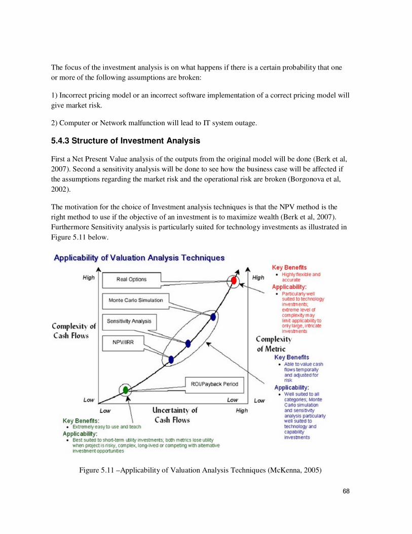
68
The focus of the investment analysis is on what happens if there is a certain probability that one
or more of the following assumptions are broken:
1) Incorrect pricing model or an incorrect software implementation of a correct pricing model will
give market risk.
2) Computer or Network malfunction will lead to IT system outage.
5.4.3 Structure of Investment Analysis
First a Net Present Value analysis of the outputs from the original model will be done (Berk et al,
2007). Second a sensitivity analysis will be done to see how the business case will be affected if
the assumptions regarding the market risk and the operational risk are broken (Borgonova et al,
2002).
The motivation for the choice of Investment analysis techniques is that the NPV method is the
right method to use if the objective of an investment is to maximize wealth (Berk et al, 2007).
Furthermore Sensitivity analysis is particularly suited for technology investments as illustrated in
Figure 5.11 below.
Figure 5.11 –Applicability of Valuation Analysis Techniques (McKenna, 2005)

69
5.4.4 Analysis – Basic reference case
To illustrate the results found in this thesis means for decision makers in the financial industry
that are deciding on how much the business should invest in an Automatic Making System a
simple example have been constructed. Assuming a Bank doing Automatic Market Making
currently is operating at network Latency level 5 with the assumed Customer Tolerance of 10, the
examples illustrates much this Bank could invest in upgrading the Algorithmic trading system to
reach a network latency level of 1 and still make a profit on the Investments.
The data illustrated in table 5.1 below can be seen for Simulation 2 in Chapter 4.4.1.
Network
latency
Average Profit (CT
=10)
1 99945
5 39722
Table 5.1 – Profitability of different levels of network latency
Assuming the maximum yearly profit of the Automatic Market Making System is 100000, as in
the model used in the simulation, the increased yearly profit for a system running at network
latency 1 compared to a system running at network latency level 5 is (99945-39722)/100000 *
100 % = 60.22%.
With an assumed Weighted Average Cost of Capital (WACC) for the Bank of 20% and an
assumed lifetime of 3 years for the Algorithmic Trading System, the maximum upfront
Investment that could be made in order for the investment to have a positive Return on
Investment, can be calculated using the Net Present Value method (Berk et al, 2007).
��� = −���� �������� + ������� �� � �� ���1
1.20+ ������� �� � �� ���
2
�1.20 ∗ 1.20�
+ Incremental return year3
�1.20 ∗ 1.20 ∗ 1.20�

70
Setting NPV = 0 to find maximum Upfront Investment to get a ROI >=0 gives:
���� ����� ��� =
������� �� � �� ���,
,.-.+ ������� �� � �� ���
-
�,.-.∗,.-.�+ Incremental return year
/
�,.-.∗,.-.∗,.-.�
Expressing the Incremental returns in percentage of the maximum yearly return for the Automatic
Market Making System gives:
= 60.22%1
1.20+ 60.22%
1
�1.20 ∗ 1.20�+ 60.22%
1
�1.20 ∗ 1.20 ∗ 1.20�= 50.18% + 41.82% + 34.85%
= 126.85%
This means that the upfront investment can be up to 126.85% of the maximum yearly profit in
order to set the Net Present Value of the investment to 0. If a smaller investment then this is
needed, it will result in a positive Net Present Value of the investment. Table 5.2 summarizes the
NPV calculation and figure 5.11 illustrates the cash flows.
Year 0 1 2 3
Cash flow -126.85% 60.22% 60.22% 60.22% Sum:
Present Value -126.85% 50.18% 41.82% 34.85% 0.00 Net Present Value for Investment
Table 5.2 - Cash flows and NPV calculation
Figure 5.12 – Cash flow diagram expressed in % of maximum yearly profit
-150.00%
-100.00%
-50.00%
0.00%
50.00%
100.00%
0 1 2 3
Year
Cashflows in % of maximum yearly profit
Present Value

71
Using the real dollar values presented in chapter 5.3.1, 126.85% of maximum yearly profit would
translate to a maximum upfront investment of between 19 and 21.5 billion USD in order to get a
positive Net Present Value of the Investment.
5.4.5 Sensitivity Analysis
Sensitivity analysis is important capital budgeting tool that breaks down the NPV calculation to
into its component assumptions and shows how the NPV varies if the underlying assumptions
change (Berk et al, 2007).
In this chapter sensitivity analysis will be used to show how the NPV calculation 5.4.4 would be
affected when market risk and operational risk are introduced. As the research was done using an
explorative modeling and simulation approach, the sensitivity analysis will also be done this way.
In addition the assumed cost of capital will be varied.
Market risk: An incorrect pricing model or an incorrect implementation of a correct pricing model
will give market risk.
Operational risk: A computer or network breakdown will give operational risk.
Table 5.3 below illustrates the input to the sensitivity analysis.
Risk Original assumption Best Case Worst Case
Market Risk 0% 0% 1-50%
Operational Risk 0% 0% 1%
Cost of Capital 20% 15% 25%
Table 5.3 – Input parameters to sensitivity analysis
Estimating realistic probabilities for worst case scenario is a complex task and would require a
separate study. One method for proper estimation of system reliability is to break down the
system into components and use Monte Carlo Simulations (Mazumber et al, 2000). In this study

72
the assumed figure of 1% for Operational risk is based on that that anything larger then this
would have been discovered during the software testing phase and would never reach production
state. For market risk, the figure could be up to 50% (random price forecasting) as quantitative
finance models are tested using historical data, financial time series, which might or might not be
representative for the future (Mills et al, 1997). A market risk of 50% means what the price
prediction model is as likely to be right as to be wrong.
In order to do the sensitivity few new assumptions needs to incorporated into the model. The
market risk could be modeled by letting 1-50% of the trades that should have become a profit
instead become a loss. The operational risk can be modeled by letting 1% of the trading days
contain no trades. Simulating a complete system shut down. Simulation 2 in Chapter 2 was run
over 100000 trades. A trading year has on average 365 – 52 * 2 = 261 trading days. This gives
100000/261 = 383 trades per day. A 1% system downtime can then be simulated by implementing
a probability that 1% of the trades are skipped.
The output from the simulation using the new risks can be seen in table 5.4 below.
Network
latency/Mar
ket Risk
Original 1% 2% 5% 10% 15% 20% 25% 50%
1 100012 98941 98911 89129 79073 69294 59355 49597 -112.9
5 38967 37753 34666 27680 15961 4542 -8555 -19307 -78587
Table 5.4 – Results from simulation including Market Risk and Operational Risk. The original model has no
market risk and no operational risk in. For the rest of the simulations the operational risk was set to 0% and the
market risk varied from 1% to 50%.
The operational risk is set to 1% throughout the whole simulation. Original model refers to the
results from the original simple model before the introduction of operational and market risk. As
clearly can be seen in table xx above the advantage of a lower network latency (1) compared to an
average network latency (5) stays with increasing market risk, unless the price prediction model

73
is wrong, or wrongly implemented. This state is represented by the market risk of 50%. At this
state the Automatic Market Making system will lose money in both cases. This is an interesting
observation as it shows that however fast the Automatic Market Making System is, it will still
lose money if the financial models behind it are incorrect or wrongly implemented in software.
Furthermore there is always a chance that this can happen as new models are typically tested on
historical. A small operational risk seems to be less important than market risk. A high
operational risk can also be avoided by proper technical software testing before the system
reaches production state.
Magnusson (2010, pers. comm.) says that the new low latency Automatic Market Making System
for Foreign Exchange Trading that UBS is currently testing in production has indeed made an
overall loss for the year of 2010 and because of this UBS is only running a small volume of the
Foreign Exchange trading over this system until it shows a profit, firstly after that UBS will move
85-95% of the volume to the Automatic Platform.
Doing a sensitivity analysis for the NPV calculation for the cost of capital based on the results
from the basic model in the same way as in chapter 5.4.4 gives the following maximal investment
sizes expressed in % of the maximum return for the various cost of capital ratios.
Cost of Capital Maximum Investment that
gives NPV>0
15% (best case) 137.5%
20% (original) 126.9%
25% (worst case) 117.6%
Table 5.5 – Maximum Upfront investment expressed in % of maximum yearly return for different
cost of capital.

74
As can be seen in Table 5.5 the upfront investment can be larger then the maximum yearly profit
for all cost of capital levels. The cost of capital can therefore be considered unimportant for this
kind of investment projects.

75
5.5 Reflections
Although the result in this thesis clearly shows that profit of an automatic market making clearly
declines with the Network latency more research would need to be done in order to deduct a more
realistic relationship between the two. The advanced extension that was developed in the second
part of this research projects also opens new questions. Will the Bank loose customers more
quickly if it uses its information about the price trend in its advantage? Or would the profit be
maximized when the Bank knows the Trend, with another customer retention model? Some
assumptions made in this thesis must probably be relaxed or modified to make a more realistic
model:
• Network latency could be modeled more realistic. In the current model it’s assumed to
always be at the defined level. In reality network latency is at a certain level most of
the time, but not all the time. Introducing a certain level of jitter and certain random
peaks would make the network latency behave more realistic.
• Further the development of the Customer Retention model should be done. First of all
the Customer Tolerance level could be made more stochastic, secondly research would
need to done to find out what a realistic level of Customer Tolerance is . Furthermore
the Customer Retention model could be extended, taking more factors into account
then in this model. This is very important as Customer Tolerance plays a critical role
in the profitability of an Automatic Market Making System, as this research clearly
shows.
By introducing Operational risk and Market risk into the model it can be observed that however
good an automatic trading system is from a technical point of view, it can still lose money if the
underlying financial models are incorrect or wrongly implemented.
Chapter 5.7 introduces ideas on how the model could be developer further.

76
5.6 Conclusions
The research done within the scope for this Thesis clearly shows that the overall profitability of
Automatic Market Making System declines with Network latency. A Bank should therefore
invest in state of the art Network infrastructure and market connections in order to maximize its
return on investments in Automatic Market Making systems. However, however good the system
is from a technical point of view, it can still lose money if the underlying financial models are
incorrect. My recommendation is therefore to first make sure that the underlying financial models
are correct, before investing in a state of the art Automatic Market Making system.
The extremely large additional profits in the billion dollar range this analysis has shown are most
not likely not realistic as it’s based on assumed profit margin of 0.25%. This figure might be very
much smaller in reality. However, the even with a 100 times smaller profit margin, the benefits of
investing in an state of the art automatic market making system is still obvious and significant.

77
5.7 Future work
5.7.1 Future extensions of model
This work is novel and among the first of its kind, it´s therefore significant scope for future work.
Some interesting ideas would be:
1. Introduce jitter to the Network Latency.
2. Let the network latency have bucket shape where a significant proportion of the latency is
at expected level, but network latency could be much higher than expected sometimes.
3. Customer Tolerance could be made more stochastic, one way to do determine if a
customer leaves or not with a random function with a certain chance that the client stays
each time it’s forced to wait. The overall Customer retention model could also be
extended to take more factors into account.
5.7.2 Future research
The result of the simulations could be compared to actual data. Two types of data would need to
be collected:
1. Daily Profit and Loss data from a specific Algorithm.
2. Daily average network latency data.
Such data will however be very difficult to collect and analyze as a typical Automatic Market
Making Algorithm uses multiple connections to multiple exchanges.
It would also be interesting to collect actual profit and network latency data and try to use
regression analysis to calculate the relationship between network latency and profit for a real
Automatic Market Making system. This kind of data is however often kept secret in Banks and
therefore this investigation would need to be done as an internal project.
The Investment scenario could also be made further realistic by using real values for Cost of
Capital and real returns from Automatic Market Making Systems operating at different levels of
Network Latency.
78
5.7.3 Improved Investment Analysis
In order to get a more accurate view of return of investments the real profit margin should be used
in the investment analysis. This figure is however a company secret within UBS so this could
only be done as an internal project within UBS.
Furthermore a more accurate estimation of system lifetime could be used and maintenance costs
before and after the upgrade could be analyzed more carefully.
5.8 Summary Chapter 5
This final chapter has analyzed and discussed the simulation results. An investment analysis
based on the NPV method on Sensitivity analyses where presented. Reflections where made and
conclusions were drawn. Proposed future research was also presented.

79
References
1. Aldridge, I (2010). High-Frequency Trading: A Practical Guide to Algorithmic Strategies
and Trading System. Wiley trading.
2. Barro, R (2008). Macroeconomics: A Modern Approach. Thomson South-Western. 2008.
3. Beattie, A. (2010). Financial Capitalism Opens Doors To Personal Fortune. Retrieved
October 16, 2010, from http://www.investopedia.com/articles/07/financial-capitalism.asp.
4. Benyon D (2010). Algorithmic trading boom creates operational risks. Retrived March
16h, 2010, from http://www.risk.net/operational-risk-and-
regulation/feature/1593030/algorithmic-trading-boom-creates-operational-risks.
5. Berk, J & DeMarzo, P (2007). Corporate Finance. Pearson.
6. Beunza B et al (2005). Tools of the trade: the socia-technology of arbitrage in a Wall
Street Trading room. Industrial and Corporate Change, Volume 13, Number 2, pp. 369-
400.
7. BIS (2001). BIS Papers No 7: Electronic finance: a new perspective and challenges,
Bank For International Settlements, Monetary and Economic Department, November
2001.
8. Borgonova E, Peccati L (2002) – University of Bocconi. Sensitivity analysis in investment
project evaluation. International Journal of Production Economics, Volume 90, Issue 1,
Pages 17-25.
9. Chaboud.A et al (2009). Rise of the Machines: Algorithmic Trading in the Foreign
Exchange Market. Board of Governnors of the Federal Reserve System, International
Finance Dicussion Papers, Number 980, October 2009.
10. Chippas T (2008). ATP Special Edition – Low Latency. Podcast. Retrieved March 16th,
2010, from http://www.algotradingpodcast.com/2008/05/16/atp-special-edition-low-
latency-featuring-thomas-chippas-deutsche-bank/.
11. Dahlgren, L. E., Lundgren, G. & Stigberg L. (2006) PENG-modellen – Värderar och ökar
nyttan av investeringar, Ekerlids Förlag, Stockholm

80
12. Dornbusch, R, Real Exchange Rates and Macroeconomics: A Selective Survey, Scand. J.
Of Economics 91 (2), 401-432, 1989.
13. Euromoney (2010). FX Survey 2010. Retrieved October 10th, 2010, from
http://www.euromoney.com/Article/2366694/FX-poll-2010-Vote-now.html.
Login/password need to be bought in order to accesss the result.
14. Gillet R et al (2009). Operational risk and reputation in the financial industry. Journal of
Banking & Finance, Volume 34, Issue 1, January 2010, pages 224-235.
15. Grant, R.M (2002). Strategy Analysis: Concepts, Techniques, Applications (4th
ed).
Blackwell publishing.
16. Houstoun et al (2009). LATENCY ROUND TABLE: The routes from L. Retrieved March
17th, 2010, from http://www.automatedtrader.net/online-exclusive/13693/latency-round-
table-the-routes-from-l.
17. Kay, R. P. Pragmatic. Pragmatic Network Latency Engineering: Fundamental Facts and
Analysis. Cpacket Networking.
18. Keat, P.G. & Young P.K.Y (2009). Managerial Economics: Economic Tools For Today´s
decision makers (6th
ed). Pearson.
19. Kendall, K (2007). Electronic and Algorithmic Trading Technology: The Complete Guide.
Elsevier
20. Klocker ( pers. comm. 2010) Interviews with Dr. Thomas Klocker, Managing Director,
Head of Algorithmic Trading FICC, UBS Investment Bank, Zürich. P.hD. from
University of Cambridhge.
21. King, J.L (2001). Operational Risk: Measurement and Modeling. Wiley Finance.
22. Khanna, A (2009). White paper: Building a Low Latency Infrastructure For Electronic
Trading. Sun Microsystems, February 2009.
23. Kolhatkar,M.G. (2009). White paper: The FX Marketplace: Trends, Opportunities and
Challenges. Infosys, January 2009.
24. Krischnawamy K.N et al, Management Research Methodology: Integration of Methods
and Techniques, Person Education India, 2009.
25. Magnusson (pers. comm. 2010), Interviews with Per Magnusson, Executive Director,
Head of FXMM IT, UBS Investment Bank, Zürich.

81
26. Mazumdar M, David E, Coit & Fen – Ru Shih (2000). A highly efficient monte carlo
method for assessment of system reliability based on a markow model. Department of
Industrial Engineering, University of Pittsburgh, 2000.
27. McHenna, P (2005). White paper: Assessing the economic value of software projects.
IBM Software Group, November 2005.
28. Michelsen P, Johnson A (2009). Beating Network Latency is crucial for High Frequency
Traders. Retrieved March 10th, 2010, from http://www.roeder-
johnson.com/RJDocs/cPacket-Says-Beating-Latency-Key-for-Algo-Traders.html.
29. Mills C.T., Markelos R.n (1997). The Econometric Modelling of Financial Time Series.
Cambridge University Press, 1997.
30. Narang, R.K (2009). Inside the Black Box: The Simple Truth about Quantitative Trading.
Wiley Finance.
31. Payne R (2003). Informed trade in spot foreign exchange markets: an empirical
investigation. Journal of International Economics, Volume 61, Issue 2, pages 307-329.
32. Porter, M.E. (reprint 2008). The Five Competitive Forces That Shape Strategy. Harvard
Business Review.
33. Power, M (2005), London School of Economics and Political Science. The invation of
operational risk. Review of International Political Economy, Volume 12, Issue 4 October
2005, pages 577-599.
34. Rockefeller (2002). The Global Trader: Strategies for Profititing in Foreign Exhange,
Futures and Stocks. Wiley Trading, 2002.
35. Saunders M & Lewis P & Thornhill A (2009). Research methods for business students (5th
Ed). Prentice Hall.
36. Smith C et al (2003). Global Banking 2nd
edition, Oxford University Press 2003.
37. Smithson, C.W (1998). Managing Financial Risk: A Guide to Derivative Products,
Financial Engineering and Value Maximization 3rd
edition, McGraw-Hill 1998.
38. Sterman, J.D. (1991). A Skeptic´s Guide to Computer Models. Westview Press.
39. Sterman, J.D. (2000). Business Dynamics: Systems Thinking and modeling for a complex
world. McGraw Hill. 2000.
40. Taleb, N.N (2007). The Black Swan: The Impact of the Highly Improbable. Penguin
Books.

82
41. Wagener et al 2010). Price efficiency in futures and spot trading: The role of information
Technology. Electronic Commerce Research and Applications, Volume 5, Issue 5,
September-October 2010, Pages 400-4009.

83
Appendix A – Source code
7.1 Price Class
using System;
using System.Collections.Generic;
using System.Linq;
using System.Text;
namespace ThesisModel
{
public class Price
{
Random m_random;
Random m_randombigperiod;
Random m_randombigsize;
Random m_trendmain;
int m_currentprice = 0;
bool m_PriceTrendUp = true;
int ticksincurrentdir = 0;
public Price(int startprice)
{
m_currentprice = startprice;
m_random = new Random();
m_randombigsize = new Random();
m_randombigperiod = new Random();
m_trendmain = new Random();
}
public bool IsPriceTrendUp()
{
return m_PriceTrendUp;
}
public int GetCurrentPrice()
{
return m_currentprice;
}

84
public int GetNextPrice(int networkdelay, bool bigmove, int bigmoveperiod,
int bigmovesize, bool usetrend, int trendperiod, int percentup)
{
if (networkdelay == 0)
{
return m_currentprice;
}
else
{
for (int i = 0; i < networkdelay; i++)
{
m_currentprice = AdjustPriceByOne(m_currentprice, bigmove,
bigmoveperiod, bigmovesize, usetrend, trendperiod, percentup);
}
return m_currentprice;
}
}
private bool MovePriceUp(int priceperiod, int percentup)
{
ticksincurrentdir++;
if (ticksincurrentdir > priceperiod)
{
if (m_PriceTrendUp)
{
m_PriceTrendUp = false;
}
else
{
m_PriceTrendUp = true;
}
ticksincurrentdir = 0;
}
int v = m_trendmain.Next(100);
if (v <= percentup)

85
{
if (m_PriceTrendUp)
{
return true;
}
else
{
return false;
}
}
else
{
if (m_PriceTrendUp)
{
return false;
}
else
{
return true;
}
}
}
private int AdjustPriceByOne(int inprice, bool bigmove, int bigmoveperiod,
int bigmovesize, bool usetrend, int pricetrendperiod, int percentageup)
{
int result = inprice;
bool up = false;
if (usetrend == false)
{
int p = m_random.Next(2);
if (p == 0)
{
up = true;
}
else
{
up = false;
}
}
else

86
{
up = MovePriceUp(pricetrendperiod, percentageup);
}
if (up)
{
if (bigmove == false)
{
result++;
}
else
{
int big = this.m_randombigperiod.Next(bigmoveperiod);
//0....period
if (big == 0)
{
//big price move happening, check size
int size = this.m_randombigsize.Next(bigmovesize);
// 5 + 0-5 default setting.
result = result + 5 + size;
}
}
}
else
{
if (bigmove == false)
{
result--;
}
else
{
int big = this.m_randombigperiod.Next(bigmoveperiod);
//0....period
int limit = bigmoveperiod / 2;
if (big == limit)
{
//big price move happening, check size
int size = this.m_randombigsize.Next(bigmovesize);
// -5 - 0-5 default setting.
result = result - 5 - size;
}

87
}
//price should not get smaller then one
if (result <= 0)
{
result = 1;
}
}
return result;
}
}
}
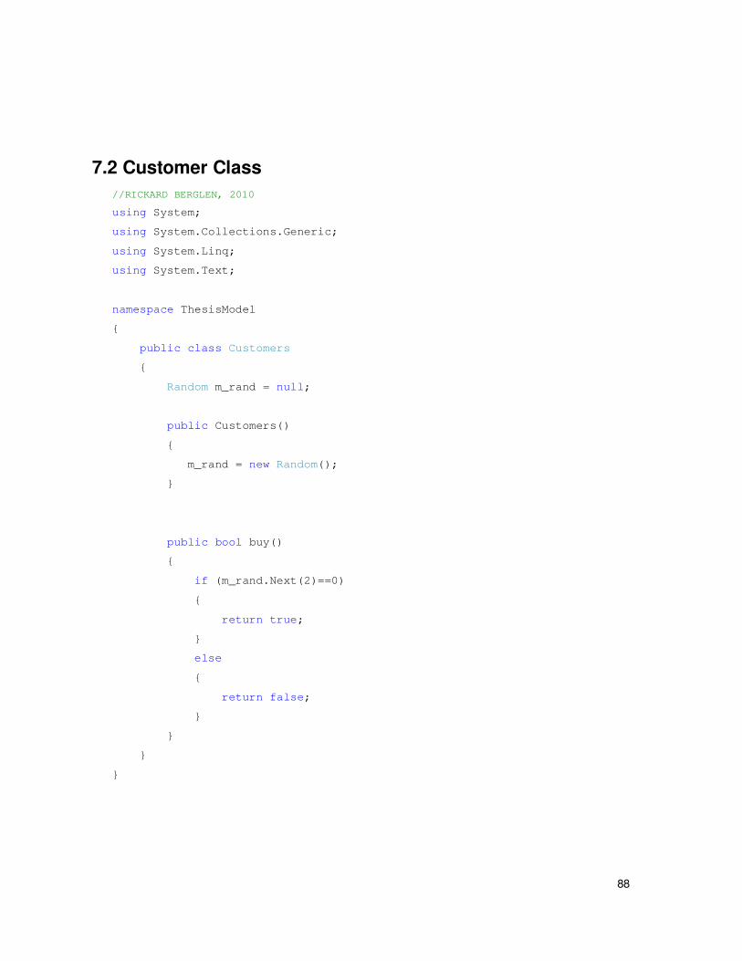
88
7.2 Customer Class
//RICKARD BERGLEN, 2010
using System;
using System.Collections.Generic;
using System.Linq;
using System.Text;
namespace ThesisModel
{
public class Customers
{
Random m_rand = null;
public Customers()
{
m_rand = new Random();
}
public bool buy()
{
if (m_rand.Next(2)==0)
{
return true;
}
else
{
return false;
}
}
}
}

89
7.3 Main program
//RICKARD BERGLEN, October 2010
using System;
using System.Collections.Generic;
using System.ComponentModel;
using System.Data;
using System.Drawing;
using System.Linq;
using System.Text;
using System.Windows.Forms;
using System.Threading;
using System.Collections;
namespace ThesisModel
{
public partial class MainApplication : Form
{
public MainApplication()
{
InitializeComponent();
}
public delegate void PrintDelegate(string msg);
public void Print(string msg)
{
this.listBoxMain.Items.Insert(0, DateTime.Now.ToString() + " " + msg);
}
public void InvokePrint(string msg)
{
this.listBoxMain.BeginInvoke(new PrintDelegate(this.Print), new
object[] { msg });
}
private Customers m_customers;
private Price m_price;
private int m_delay = 0;
private int m_nr_customers = 0;
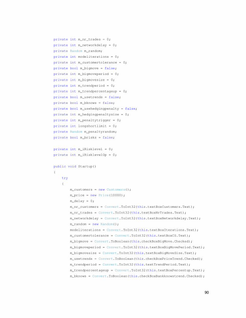
90
private int m_nr_trades = 0;
private int m_networkdelay = 0;
private Random m_random;
private int modeliterations = 0;
private int m_customertolerance = 0;
private bool m_bigmove = false;
private int m_bigmoveperiod = 0;
private int m_bigmovesize = 0;
private int m_trendperiod = 0;
private int m_trendpercentageup = 0;
private bool m_usetrends = false;
private bool m_bknows = false;
private bool m_usehedgingpenalty = false;
private int m_hedgingpenaltysize = 0;
private int m_penaltytrigger = 0;
private int longshortlimit = 0;
private Random m_penaltyrandom;
private bool m_brisks = false;
private int m_iRisklevel = 0;
private int m_iRisklevelOp = 0;
public void Startup()
{
try
{
m_customers = new Customers();
m_price = new Price(10000);
m_delay = 0;
m_nr_customers = Convert.ToInt32(this.textBoxCustomers.Text);
m_nr_trades = Convert.ToInt32(this.textBoxNrTrades.Text);
m_networkdelay = Convert.ToInt32(this.textBoxNetworkdelay.Text);
m_random = new Random();
modeliterations = Convert.ToInt32(this.textBoxIterations.Text);
m_customertolerance = Convert.ToInt32(this.textBoxCS.Text);
m_bigmove = Convert.ToBoolean(this.checkBoxBigMove.Checked);
m_bigmoveperiod = Convert.ToInt32(this.textBoxBigMovePeriod.Text);
m_bigmovesize = Convert.ToInt32(this.textBoxBigMoveSize.Text);
m_usetrends = Convert.ToBoolean(this.checkBoxPriceTrend.Checked);
m_trendperiod = Convert.ToInt32(this.textTrendPeriod.Text);
m_trendpercentageup = Convert.ToInt32(this.textBoxPercentup.Text);
m_bknows = Convert.ToBoolean(this.checkBoxBankknowstrend.Checked);

91
m_usehedgingpenalty =
Convert.ToBoolean(this.checkBoxEnableExpensiveHedging.Checked);
m_hedgingpenaltysize =
Convert.ToInt32(this.textBoxHedgePenalty.Text);
m_penaltytrigger =
Convert.ToInt32(this.textBoxPenaltytrigger.Text);
longshortlimit = Convert.ToInt32(this.textBoxLongShortLimit.Text);
m_brisks = Convert.ToBoolean(this.checkBoxRisks.Checked);
m_iRisklevel = Convert.ToInt32(this.textBoxrisklevel.Text);
m_iRisklevelOp = Convert.ToInt32(this.textBoxOprisk.Text);
m_penaltyrandom = new Random();
backgroundWorkerRun.RunWorkerAsync();
}
catch (Exception ex)
{
MessageBox.Show(ex.Message);
}
}
private void buttonStart_Click(object sender, EventArgs e)
{
try
{
Startup();
}
catch (Exception ex)
{
MessageBox.Show(ex.Message);
}
}
private void backgroundWorkerRun_DoWork(object sender, DoWorkEventArgs e)
{
RunModell(sender as BackgroundWorker, e);
}
private void RunModell(BackgroundWorker worker, DoWorkEventArgs e)
{
try
{

92
int profit = 0;
int clientprice = 0;
int bankprice = 0;
int marketprice = 0;
int nrbuy = 0;
int nrsell = 0;
double propbuy = 0.0;
int totalticks = m_nr_customers * m_nr_trades * 2;
int orgcustomers = m_nr_customers;
int iterationsrun = 0;
int longcounter = 0;
int shortcounter = 0;
int i = 0;
int customer_tolerenace = m_customertolerance;
int customer_hits = 0;
int totaltrades = 0;
int tradesthisrun = 0;
double averageprofit = 0;
double profitpertrade = 0;
double averageiterations = 0;
double averagecustomers = 0;
double averagemarketprice = 0;
int currenthedgepenalty = 0;
//more realistic, sortable array....
Queue<int> m_buyprices = new Queue<int>();
Queue<int> m_sellprices = new Queue<int>();
for (int iterations = 0; iterations < modeliterations;
iterations++)
{
profit = 0;
nrbuy = 0;
nrsell = 0;
m_nr_customers = orgcustomers;

93
iterationsrun = 0;
tradesthisrun = 0;
for (i = 0; i < totalticks; i++)
{
//Operational risk
if (m_brisks == true)
{
//one chance in 100
if (m_random.Next(100) < m_iRisklevelOp)
{
continue;
}
}
iterationsrun++;
if (worker.CancellationPending == true)
{
break;
}
//clock
//0 == price change, 1 = trade
int priceChangeOrTrade = m_random.Next(2);
if (priceChangeOrTrade == 0)
{
//PRICE MOVE
m_price.GetNextPrice(m_networkdelay,m_bigmove,m_bigmoveperiod,m_bigmovesize,m_usetr
ends,m_trendperiod,m_trendpercentageup);
}
else
{
//TRADE
tradesthisrun++;
marketprice = m_price.GetCurrentPrice();
//BUY
if (m_customers.buy() == true)
{
//CLIENT WANT TO BUY => We SELL
clientprice = marketprice + 1; // point 5

94
nrbuy++;
//if we are too short, hedge away all short
positions
if (shortcounter == longshortlimit)
{
for (int j = 0; j < longshortlimit; j++)
{
//market price will move, depending on latency
marketprice =
m_price.GetNextPrice(m_networkdelay, m_bigmove, m_bigmoveperiod, m_bigmovesize,
m_usetrends, m_trendperiod, m_trendpercentageup);
//Our price will be the price we sold earlier
at
bankprice = m_sellprices.Dequeue();
//we buy, to market price
//profit if we sold more expensive before
//1. BUY at market price
//2. If price we sold to clients to before is
bigger then what we pay now, profit
int incprofit = bankprice - marketprice;
profit = profit + incprofit;
//market risk - 1%
if (m_brisks == true)
{
if (incprofit > 0)
{
if (m_random.Next(100) < m_iRisklevel)
{
profit = profit - incprofit -
incprofit;
}
}
}

95
}
//Sell to the client, after the hedging
m_sellprices.Enqueue(clientprice);
shortcounter = 1;
customer_hits++;
if (customer_hits >= customer_tolerenace)
{
//loose one customer
m_nr_customers--;
i = i + m_nr_trades;
customer_hits = 0;
}
}
else
{
//Try to Sell and hedge away directly
//Get bank BUY price on hedge exchange
bankprice =
m_price.GetNextPrice(m_networkdelay, m_bigmove, m_bigmoveperiod, m_bigmovesize,
m_usetrends, m_trendperiod, m_trendpercentageup);
//Bank knows trend....if bank is selling, and
needs to buy back later...always buy directly if price trend is upwards, never buy
directly if price
//trend is down - cheaper later - but trend
might change
if (m_usetrends == true)
{
if (m_bknows == true)
{
if (m_price.IsPriceTrendUp() == true)
{
//more expensive later, hedge now
int incprofit = clientprice -
bankprice;

96
profit = profit + incprofit;
//market risk - 1%
if (m_brisks == true)
{
if (incprofit > 0)
{
if (m_random.Next(100) <
m_iRisklevel)
{
profit = profit -
incprofit - incprofit;
}
}
}
}
else
{
//trade directly, hedge
later,cheaper later
m_sellprices.Enqueue(clientprice);
shortcounter++;
}
}
else
{
//If bankprice <= client price, trade
directly, cash profit
if (bankprice <= clientprice)
{
int incprofit = clientprice -
bankprice;
profit = profit + incprofit;
//market risk - 1%
if (m_brisks == true)
{
if (incprofit > 0)
{

97
if (m_random.Next(100) <
m_iRisklevel)
{
profit = profit -
incprofit - incprofit;
}
}
}
}
else
{
//Else, hedge later
m_sellprices.Enqueue(clientprice);
shortcounter++;
}
}
}
else
{
//If bankprice <= client price, trade
directly, cash profit
if (bankprice <= clientprice)
{
int incprofit = clientprice -
bankprice;
profit = profit + incprofit;
//market risk - 1%
if (m_brisks == true)
{
if (incprofit > 0)
{
if (m_random.Next(100) <
m_iRisklevel)
{
profit = profit - incprofit
- incprofit;
}
}
}

98
}
else
{
//Else, hedge later
m_sellprices.Enqueue(clientprice);
shortcounter++;
}
}
}
}
else
{
//CLIENT WANT TO SELL, WE BUY
nrsell++;
clientprice = marketprice - 1;
if (longcounter == longshortlimit)
{
//we reached the max long limit
//hedge out to current marketprice
for (int j = 0; j < longshortlimit; j++)
{
//Take a price from our long positions,
sell to market price
bankprice = m_buyprices.Dequeue();
//market price will move, depending on
latency
marketprice =
m_price.GetNextPrice(m_networkdelay, m_bigmove, m_bigmoveperiod, m_bigmovesize,
m_usetrends, m_trendperiod, m_trendpercentageup);
//we sell, to market price
int incprofit = marketprice - bankprice;
profit = profit + incprofit;
//market risk - 1%

99
if (m_brisks == true)
{
if (incprofit > 0)
{
if (m_random.Next(100) <
m_iRisklevel)
{
profit = profit - incprofit -
incprofit;
}
}
}
}
longcounter = 0;
//BUY FROM CLIENT, KEEP POSITION
m_buyprices.Enqueue(clientprice);
longcounter = 1;
customer_hits++;
//loose one customer
if (customer_hits >= customer_tolerenace)
{
m_nr_customers--;
i = i + m_nr_trades*2;
customer_hits = 0;
}
}
else
{
bankprice =
m_price.GetNextPrice(m_networkdelay, m_bigmove, m_bigmoveperiod, m_bigmovesize,
m_usetrends, m_trendperiod, m_trendpercentageup);
//Bank knows trend....if bank is buying, and
need to sell later....sell directly if price trend is down, get less money later,
sell later, if price trend is up
if (m_usetrends == true)
{
if (m_bknows == true)

100
{
if (m_price.IsPriceTrendUp() == true)
{
//BUY from client, keep position -
will get more later
m_buyprices.Enqueue(clientprice);
longcounter++;
}
else
{
//sell directly, get less later.
int incprofit = bankprice -
clientprice;
profit = profit + incprofit;
//market risk - 1%
if (m_brisks == true)
{
if (incprofit > 0)
{
if (m_random.Next(100) <
m_iRisklevel)
{
profit = profit -
incprofit - incprofit;
}
}
}
}
}
else
{
//we hedge directly if we get can SELL
more expensive then client BUY from us at
if (bankprice >= clientprice)
{
//BUY from client, hedge directly.
int incprofit = bankprice -
clientprice;
profit = profit + incprofit;

101
//market risk - 1%
if (m_brisks == true)
{
if (incprofit > 0)
{
if (m_random.Next(100) <
m_iRisklevel)
{
profit = profit -
incprofit - incprofit;
}
}
}
}
else
{
//BUY from client, keep position
m_buyprices.Enqueue(clientprice);
longcounter++;
}
}
}
else
{
//we hedge directly if we get can SELL more
expensive then client BUY from us at
if (bankprice >= clientprice)
{
//BUY from client, hedge directly.
int incprofit = bankprice -
clientprice;
profit = profit + incprofit;
//market risk - 1%
if (m_brisks == true)
{
if (incprofit > 0)
{

102
if (m_random.Next(100) <
m_iRisklevel)
{
profit = profit - incprofit
- incprofit;
}
}
}
}
else
{
//BUY from client, keep position
m_buyprices.Enqueue(clientprice);
longcounter++;
}
}
}
}
//when we trade and and have hedging penalty enabled...
if (m_usehedgingpenalty == true)
{
int penaltyhit =
m_penaltyrandom.Next(m_networkdelay);
//if 0 - we don't get penaly => chances of penalty
increases with network latency
if (penaltyhit != 0)
{
currenthedgepenalty++;
if (currenthedgepenalty >= m_penaltytrigger)
{
profit = profit - m_hedgingpenaltysize;
currenthedgepenalty = 0;
}
}
}
}

103
if (nrbuy > 0 && nrsell > 0)
{
propbuy = Convert.ToDouble(nrbuy) /
Convert.ToDouble((nrbuy + nrsell));
propbuy = Math.Round(propbuy, 2);
}
double progress = Convert.ToDouble(i) /
Convert.ToDouble(totalticks) * 100;
progress = Math.Round(progress, 0);
int iprogress = Convert.ToInt32(progress);
//worker.ReportProgress(iprogress);
if (m_nr_customers <= 0)
{
break;
}
Thread.Sleep(m_delay);
}
//InvokePrint("Buy(%):" + propbuy.ToString());
//InvokePrint("Profit: " + profit.ToString());
InvokePrint("Iterations run: " + iterationsrun.ToString() + "
out of " + totalticks);
averageprofit = averageprofit + Convert.ToDouble(profit);
averagecustomers = averagecustomers +
Convert.ToDouble(m_nr_customers);
averageiterations = averageiterations + iterationsrun;
averagemarketprice = averagemarketprice +
Convert.ToDouble(m_price.GetCurrentPrice());
totaltrades += tradesthisrun;
}
averageprofit = averageprofit / modeliterations;
double averagenrtrades = totaltrades / modeliterations;
profitpertrade = averageprofit / averagenrtrades;
averagecustomers = averagecustomers / modeliterations;
averageiterations = averageiterations / modeliterations;

104
averagemarketprice = averagemarketprice / modeliterations;
InvokePrint(propbuy.ToString());
//InvokePrint("Model Iterations:" + iterations.ToString());
InvokePrint("Average Price: " + averagemarketprice.ToString());
InvokePrint("Average Profit: " + averageprofit.ToString());
InvokePrint("Average trade per simulation run: " +
averagenrtrades.ToString());
InvokePrint("Profit per trade: " + profitpertrade.ToString());
InvokePrint("Average Customers left: " +
averagecustomers.ToString());
InvokePrint("Average iterations: " + averageiterations.ToString());
}
catch (Exception ex)
{
InvokePrint("Model failed: " + ex.Message);
}
}
private void backgroundWorkerRun_RunWorkerCompleted(object sender,
RunWorkerCompletedEventArgs e)
{
Print("Simulation finished");
}
private void buttonStop_Click(object sender, EventArgs e)
{
this.backgroundWorkerRun.CancelAsync();
}
}
}