Embed Size (px)
Citation preview
Automatic Detection of Cancer in Lymph
Nodes
Liam Mulvey
Computer Science2008/09
The candidate confirms that the work submitted is their own and the appropriate credit has been given
where reference has been made to the work of others.
I understand that failure to attribute material which is obtained from another source may be considered
as plagiarism.
(Signature of student)
Summary
The discipline of computer vision provides many advantages for a wide selection of industries,
including the medical profession. Currently, pathologists take tissue samples and biopsies which are
used to create slides to be viewed under a microscope. These slides are then analysed and the results
interpreted to check for various diseases and conditions. Using modern imaging technology, these slides
can be used to create digital images of very high resolutions. Virtual pathology is the study of these
images, with the aim of providing automatic medical diagnoses which can aid doctors in discerning
whether a patient has a specific ailment.
At present, this discipline is very much in its infancy. The aim of this project is to examine previous
research in this area and build upon it to create a system that can analyse images of these slides and
attempt a diagnosis.
i
Acknowledgements
I’d like to thank the following people:
• My supervisor, Andy Bulpitt, for his aid and support over this year.
• Derek Magee for his endless help in all matters concerned with this project.
• Darren Treanor for all his patient explanations of the science of pathology.
• Ken Brodlie for his useful feedback on my mid-project report and his fantastic input in the project
demonstration.
I’d also like to thank:
• Chris Clarke for proof-reading this report and catching some of my more idiotic mistakes!
• Everyone who lived in the lab over the past few weeks. You know who you are.
• Ed for providing me with hours of entertainment as he rants about voting.
And finally, I’d like to thank Roisin and everyone else who put up with my complaining about this
project.
ii
Contents
1 Project Introduction 1
1.1 Introduction . . . . . . . . . . . . . . . . . . . . . . . . . . . . . . . . . . . . . . . . 1
1.2 Aim . . . . . . . . . . . . . . . . . . . . . . . . . . . . . . . . . . . . . . . . . . . . 1
1.3 Objectives . . . . . . . . . . . . . . . . . . . . . . . . . . . . . . . . . . . . . . . . . 2
1.4 Minimum Requirements . . . . . . . . . . . . . . . . . . . . . . . . . . . . . . . . . 2
1.5 Medical Terminology . . . . . . . . . . . . . . . . . . . . . . . . . . . . . . . . . . . 2
2 Project Management 4
2.1 Overview . . . . . . . . . . . . . . . . . . . . . . . . . . . . . . . . . . . . . . . . . 4
3 Background Research 7
3.1 Histopathology . . . . . . . . . . . . . . . . . . . . . . . . . . . . . . . . . . . . . . 7
3.2 Cancer . . . . . . . . . . . . . . . . . . . . . . . . . . . . . . . . . . . . . . . . . . . 8
3.2.1 Colorectal Cancer . . . . . . . . . . . . . . . . . . . . . . . . . . . . . . . . . 8
3.3 Cell Biology and Structure . . . . . . . . . . . . . . . . . . . . . . . . . . . . . . . . 9
3.4 Cancer Detection . . . . . . . . . . . . . . . . . . . . . . . . . . . . . . . . . . . . . 11
3.5 Colour Deconvolution . . . . . . . . . . . . . . . . . . . . . . . . . . . . . . . . . . . 15
3.6 Nuclear Detection . . . . . . . . . . . . . . . . . . . . . . . . . . . . . . . . . . . . . 16
3.7 Delaunay Triangulation . . . . . . . . . . . . . . . . . . . . . . . . . . . . . . . . . . 17
3.8 Current Solutions . . . . . . . . . . . . . . . . . . . . . . . . . . . . . . . . . . . . . 18
4 Design and Implementation 19
4.1 Research . . . . . . . . . . . . . . . . . . . . . . . . . . . . . . . . . . . . . . . . . . 19
4.1.1 Usable Technologies . . . . . . . . . . . . . . . . . . . . . . . . . . . . . . . 20
iii
4.1.1.1 Matlab . . . . . . . . . . . . . . . . . . . . . . . . . . . . . . . . . 20
4.1.1.2 C/C++ . . . . . . . . . . . . . . . . . . . . . . . . . . . . . . . . . 21
4.1.1.3 Java and Python . . . . . . . . . . . . . . . . . . . . . . . . . . . . 21
4.1.1.4 OpenCV . . . . . . . . . . . . . . . . . . . . . . . . . . . . . . . . 21
4.1.1.5 Aperio Image Server . . . . . . . . . . . . . . . . . . . . . . . . . . 22
4.2 Performance Issues . . . . . . . . . . . . . . . . . . . . . . . . . . . . . . . . . . . . 23
4.2.1 Image Size . . . . . . . . . . . . . . . . . . . . . . . . . . . . . . . . . . . . 23
4.3 Proposed Resources . . . . . . . . . . . . . . . . . . . . . . . . . . . . . . . . . . . . 24
4.4 Image Retrieval . . . . . . . . . . . . . . . . . . . . . . . . . . . . . . . . . . . . . . 25
4.5 Node Extraction . . . . . . . . . . . . . . . . . . . . . . . . . . . . . . . . . . . . . . 25
4.6 Feature Extraction . . . . . . . . . . . . . . . . . . . . . . . . . . . . . . . . . . . . . 27
4.6.1 Nuclear Detection . . . . . . . . . . . . . . . . . . . . . . . . . . . . . . . . 27
4.6.2 Delaunay Triangulation . . . . . . . . . . . . . . . . . . . . . . . . . . . . . . 28
4.7 Colour Analysis . . . . . . . . . . . . . . . . . . . . . . . . . . . . . . . . . . . . . . 30
4.8 Diagnosis . . . . . . . . . . . . . . . . . . . . . . . . . . . . . . . . . . . . . . . . . 31
4.9 Problems Encountered . . . . . . . . . . . . . . . . . . . . . . . . . . . . . . . . . . 32
5 Results Analysis 33
5.1 Programme Results . . . . . . . . . . . . . . . . . . . . . . . . . . . . . . . . . . . . 33
6 Evaluation 36
6.1 Image Retrieval . . . . . . . . . . . . . . . . . . . . . . . . . . . . . . . . . . . . . . 36
6.2 Nuclear Detection . . . . . . . . . . . . . . . . . . . . . . . . . . . . . . . . . . . . . 38
6.3 Delaunay Triangulation . . . . . . . . . . . . . . . . . . . . . . . . . . . . . . . . . . 40
6.4 Colour Analysis . . . . . . . . . . . . . . . . . . . . . . . . . . . . . . . . . . . . . . 40
6.5 System Evaluation . . . . . . . . . . . . . . . . . . . . . . . . . . . . . . . . . . . . 41
6.6 Future Improvements . . . . . . . . . . . . . . . . . . . . . . . . . . . . . . . . . . . 41
6.6.1 Machine Learning . . . . . . . . . . . . . . . . . . . . . . . . . . . . . . . . 42
6.6.2 Extra Features . . . . . . . . . . . . . . . . . . . . . . . . . . . . . . . . . . 42
6.7 Conclusion . . . . . . . . . . . . . . . . . . . . . . . . . . . . . . . . . . . . . . . . 43
Bibliography 44
iv

A Personal Reflection 46
v
Chapter 1
Project Introduction
1.1 Introduction
Detection is a crucial stage for the treatment of cancer patients. Usually, the earlier the cancer can be
detected, the better chance the patient has of going into remission and surviving the disease. Pathol-
ogists view thousands of slide a year, however the time taken to set up the slides and analyse them
by hand means that this is not overly efficient. The next advancement would be automatic detection
software. This would reduce the input necessary from the pathologists and would then contribute to a
higher turnover of slides. Whilst no automated system could be trusted explicitly at this stage, the results
coming from the system could alert the pathologist to any areas where the cancer is likely to be found.
This would again increase the rate at which the pathologist could check the slides and make diagnoses.
1.2 Aim
The aim of this project is to analyse digital slides of lymph node samples for cancer development.
Current methods mean that pathologists have to check each slide manually. This project is looking at
methods for automatically analysing and detecting any cancerous cells present in the samples.
1
1.3 Objectives
The objectives of the project are to:
• Research the current technology and techniques used;
• Research the behaviour of cancerous growths in lymph nodes. This would allow key insight into
how the pathologist analyses the tissue samples for cancerous growths. In turn, this would provide
a basis for the necessary software capabilities.
• Investigate the relevant techniques in computer vision for use in a cancer detection scheme;
• Develop a system to classify slides as normal or cancerous;
• Compare the achieved results with those of a human pathologist;
• Evaluate the successfulness of the solution.
1.4 Minimum Requirements
The minimum requirements are:
• A program which can locate the lymph nodes present on a digital image of a tissue sample.
• A program to locate areas of cancer and notify the user of the presence of cancer in the relevant
slides.
The possible extensions are:
• A program which can highlight the affected areas of the sample.
1.5 Medical Terminology
This is a list of the medical terms used in the document:
• Haematoxylin and Eosin - This is the particular stain used in pathology for the diagnosis of cancer.
It is often referred to as H&E or H+E.
2
• Nucleus - The nucleus is the section of the cell which contains the majority of the DNA and RNA
necessary for cell replication and operation. These sections appear purple when the slides are
stained using H&E.
• DNA - Deoxyribonucleic acid. This is the nucleic acid present in the nucleus which contains the
genetic information that codes for all the necessary components of a cell e.g. proteins.
• RNA - Ribonucleic acid. This is coded from the DNA molecules present in the nucleus and is
crucial to the creation of the proteins necessary for the cells function.
• Eukaryotic cell - A cell with a nucleus.
• Cytoplasm - This makes up the remainder of the cell. It is a jelly-like substance of approximately
eighty percent water which containes the organelles necessary for the operation of the cell. The
cytoplasm appears pink when stained.
• Histopathology - The process of diagnosing patients by studying samples of tissue from the pa-
tient.
• Biopsy - A medical test using the removal of cells or tissue for study.
• Polyp - An abnormal tissue growth originating from a mucus membrane.
• Adenoma - A collection of glandular growths.
• Epithelial cells - Secretion cells. Multiple epithelial cells make up the glands present in the body.
• Metastasis - The name given to a cancer that has spread to another section of the body. Also
known as a secondary cancer.
3
Chapter 2
Project Management
2.1 Overview
This section outlines the process behind managing this project. The first semester was concerned mainly
with understanding the problem, background research and familiarisation with the possible technolo-
gies. The main fields of the background research were the biological aspects of the project, current
techniques used in this field and previous studies into visual pathology. The biological basics were the
crucial starting point and so these were the first aspects to be concentrated on. After three weeks, the
main focus moved on to the previous studies and gradually moved onto the current useful methods.
During this semester weekly meetings were held to review the research findings and any practical work
that had been carried out. At the end of the first semester a mid-project report was submitted outlining
the problem, the research carried out and the desired direction of the project. The second semester had
more rigid deadlines as certain aspects of the programme needed to be developed and tested to produce
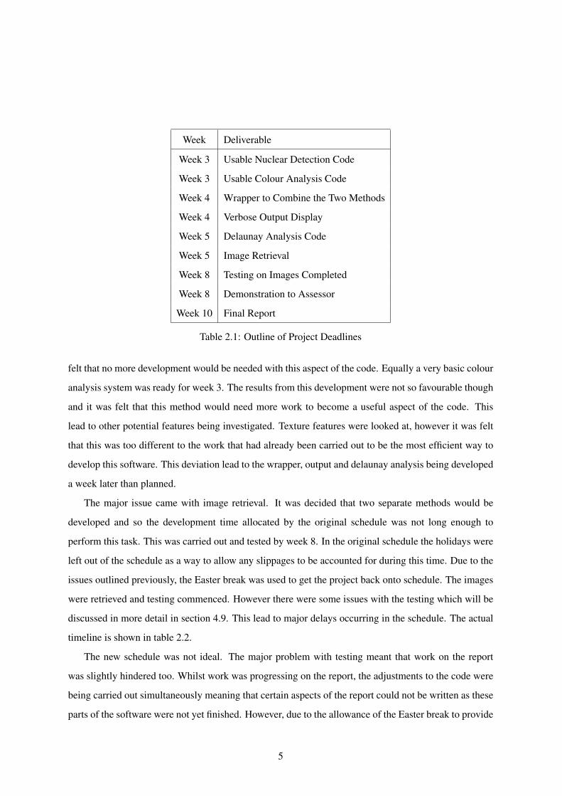
the final version of the system. Table 2.1 outlines the desired schedule for the semester.
Unfortunately, as with any software development project, whilst the greatest effort was made to
stick to this schedule, unforeseen problems caused aspects to slip off schedule. The first deliverable
was met and the nuclear detection code was tested on multiple images to ascertain whether any extra
development was to be needed on the code. The results from these tests were favourable and so it was
4
Week Deliverable
Week 3 Usable Nuclear Detection Code
Week 3 Usable Colour Analysis Code
Week 4 Wrapper to Combine the Two Methods
Week 4 Verbose Output Display
Week 5 Delaunay Analysis Code
Week 5 Image Retrieval
Week 8 Testing on Images Completed
Week 8 Demonstration to Assessor
Week 10 Final Report
Table 2.1: Outline of Project Deadlines
felt that no more development would be needed with this aspect of the code. Equally a very basic colour
analysis system was ready for week 3. The results from this development were not so favourable though
and it was felt that this method would need more work to become a useful aspect of the code. This
lead to other potential features being investigated. Texture features were looked at, however it was felt
that this was too different to the work that had already been carried out to be the most efficient way to
develop this software. This deviation lead to the wrapper, output and delaunay analysis being developed
a week later than planned.
The major issue came with image retrieval. It was decided that two separate methods would be
developed and so the development time allocated by the original schedule was not long enough to
perform this task. This was carried out and tested by week 8. In the original schedule the holidays were
left out of the schedule as a way to allow any slippages to be accounted for during this time. Due to the
issues outlined previously, the Easter break was used to get the project back onto schedule. The images
were retrieved and testing commenced. However there were some issues with the testing which will be
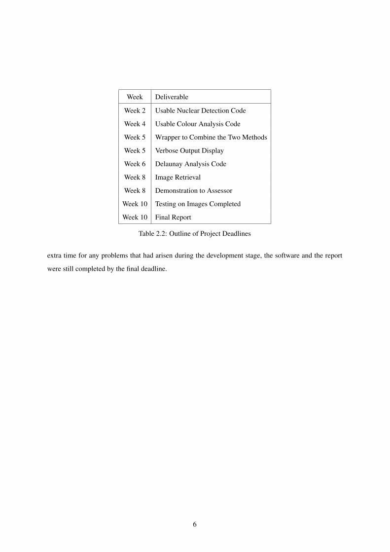
discussed in more detail in section 4.9. This lead to major delays occurring in the schedule. The actual
timeline is shown in table 2.2.
The new schedule was not ideal. The major problem with testing meant that work on the report
was slightly hindered too. Whilst work was progressing on the report, the adjustments to the code were
being carried out simultaneously meaning that certain aspects of the report could not be written as these
parts of the software were not yet finished. However, due to the allowance of the Easter break to provide
5
Week Deliverable
Week 2 Usable Nuclear Detection Code
Week 4 Usable Colour Analysis Code
Week 5 Wrapper to Combine the Two Methods
Week 5 Verbose Output Display
Week 6 Delaunay Analysis Code
Week 8 Image Retrieval
Week 8 Demonstration to Assessor
Week 10 Testing on Images Completed
Week 10 Final Report
Table 2.2: Outline of Project Deadlines
extra time for any problems that had arisen during the development stage, the software and the report
were still completed by the final deadline.
6
Chapter 3
Background Research
3.1 Histopathology
Histopathology is concerned with the study of human tissue samples. Traditionally, pathologists would
study these samples using a light microscope. However, with the latest technological advances, pathol-
ogists can now digitise these slides into high resolution images which has led to automated solutions
being sought to aid pathologists in their work. Pathologists make their diagnosis through studying the
cell structures present in the samples. This is covered in more detail in section 3.3. However there are
some issues with the discipline of pathology. One major issue is that there are no set rules for diagnosis,
thus the art of pathology is a subjective discipline. Whilst there can be definite cases, both negative and
positive, the less clear cases can be diagnosed differently by different pathologists. On average, two
equally experienced pathologists will only agree roughly eighty five percent of the time. This has led
to efforts being made to look into creating some quantitative guidelines and subsequently this area is
where the majority of automated pathology projects are looking.
7
3.2 Cancer
Cancer is one of the major causes of premature death in the world. In 2004, cancer alone accounted for
7.4 million deaths; roughly 13% of all deaths worldwide [18]. Cancer refers to any malignant growth
caused by abnormal and uncontrollable cell division. There are a great many causes of cancer including:
• Chemical carcinogens
• Age
• Diet and alcohol consumption
• Radiation
• Infection
• Auto-immune deficiencies
• Hereditary
Chemical carcinogens include cigarette smoke, asbestos, benzene and formaldehyde. Unprotected
exposure to these increase the chance of cancer developing. Cigarette smoke is estimated to be the main
cause of around 25% of all cancers with 1 in 10 of these being lung cancer.
3.2.1 Colorectal Cancer
This project is concerned with the detection of colorectal cancer in lymph nodes. This is the third high-
est cause of cancerous deaths in the UK [18] with 639,000 deaths from this particular type. Colorectal
cancer is thought to be caused by adenoma polyps which grow from the epithelial cells present in the
colon. These polyps are normally benign however they can develop into malignant tumours. These are
the growths referred to as colorectal cancer.
8
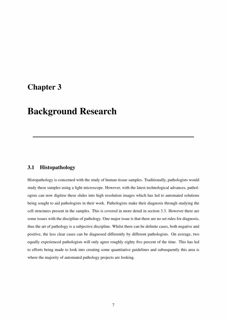
3.3 Cell Biology and Structure
A standard animal cell consists of three main components. These are:
• Nucleus
• Cell membrane
• Cytoplasm
Figure 3.1: Representation of an Animal Cell [15]
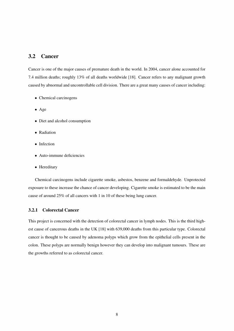
The nucleus is the most prominent structure in the cell and contains the DNA and RNA necessary
for cell replication. In a normal eukaryotic cell, the nucleic acids are tightly packed in a regular layered
structure. In a healthy lymph node, these nuclei are between five and six micrometers and are surrounded
by minimal cytoplasm and the cell membrane. On a slide these appear to be a large circle with a border.
The cell structure is illustrated in figure 3.2.
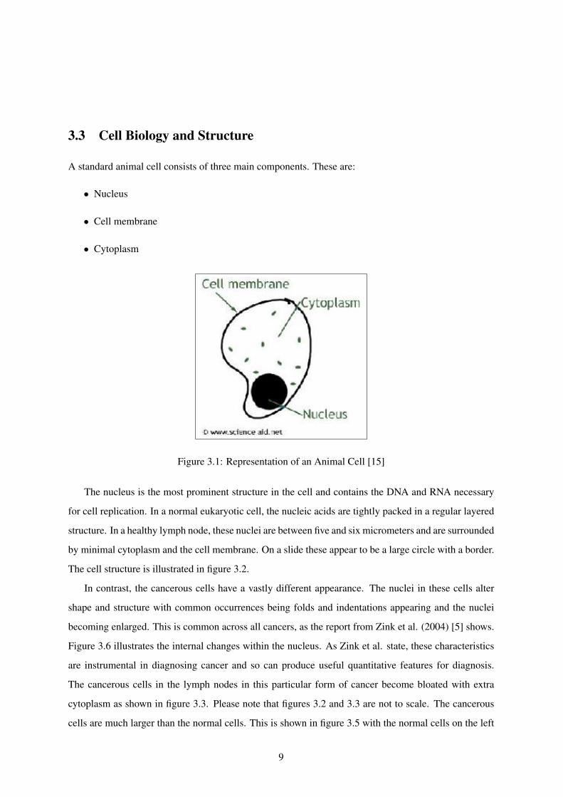
In contrast, the cancerous cells have a vastly different appearance. The nuclei in these cells alter
shape and structure with common occurrences being folds and indentations appearing and the nuclei
becoming enlarged. This is common across all cancers, as the report from Zink et al. (2004) [5] shows.
Figure 3.6 illustrates the internal changes within the nucleus. As Zink et al. state, these characteristics
are instrumental in diagnosing cancer and so can produce useful quantitative features for diagnosis.
The cancerous cells in the lymph nodes in this particular form of cancer become bloated with extra
cytoplasm as shown in figure 3.3. Please note that figures 3.2 and 3.3 are not to scale. The cancerous
cells are much larger than the normal cells. This is shown in figure 3.5 with the normal cells on the left
9
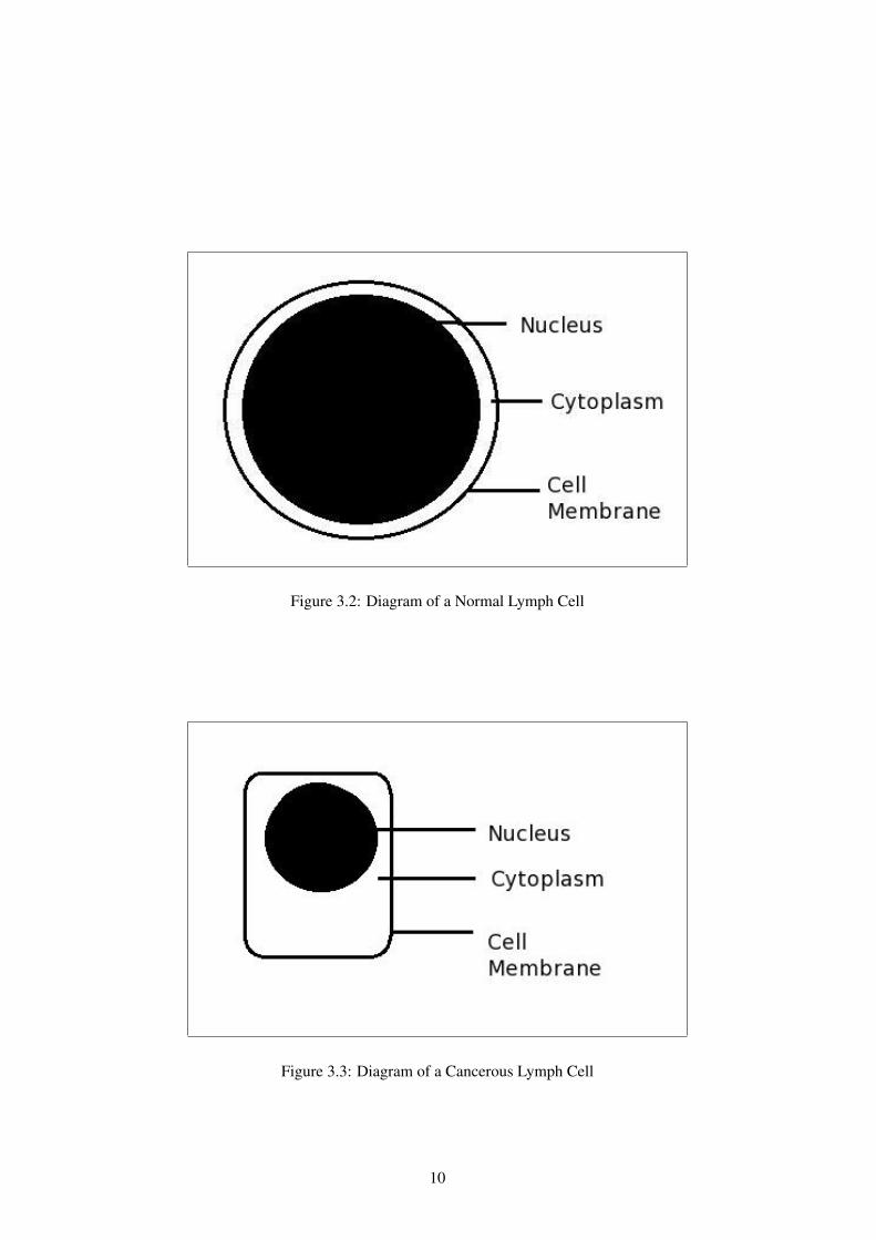
Figure 3.2: Diagram of a Normal Lymph Cell
Figure 3.3: Diagram of a Cancerous Lymph Cell
10
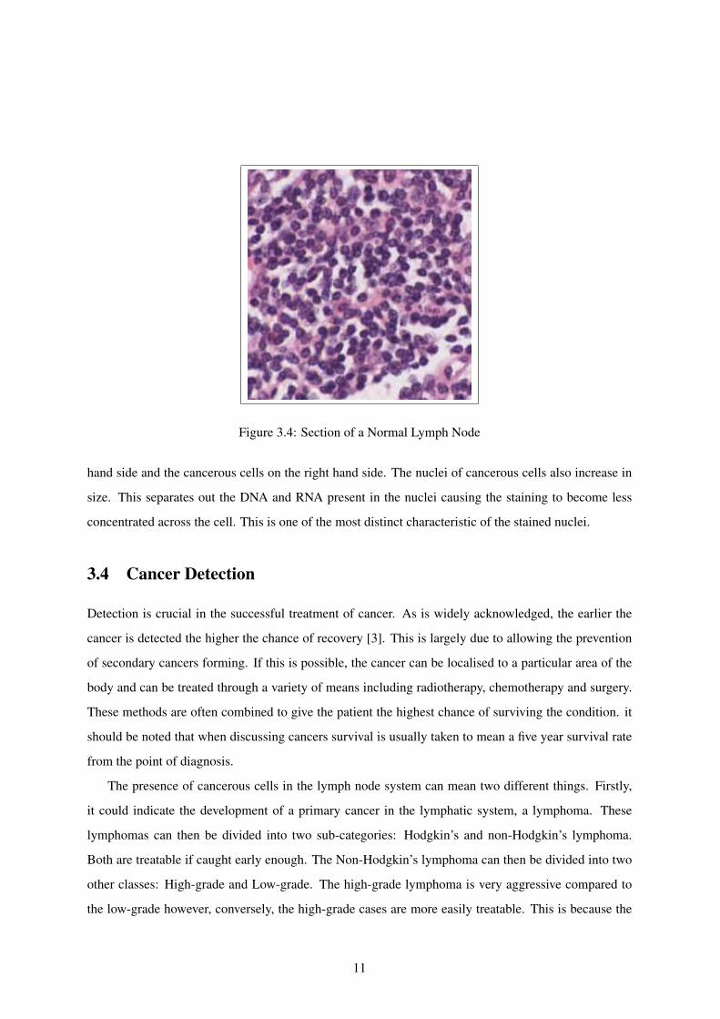
Figure 3.4: Section of a Normal Lymph Node
hand side and the cancerous cells on the right hand side. The nuclei of cancerous cells also increase in
size. This separates out the DNA and RNA present in the nuclei causing the staining to become less
concentrated across the cell. This is one of the most distinct characteristic of the stained nuclei.
3.4 Cancer Detection
Detection is crucial in the successful treatment of cancer. As is widely acknowledged, the earlier the
cancer is detected the higher the chance of recovery [3]. This is largely due to allowing the prevention
of secondary cancers forming. If this is possible, the cancer can be localised to a particular area of the
body and can be treated through a variety of means including radiotherapy, chemotherapy and surgery.
These methods are often combined to give the patient the highest chance of surviving the condition. it
should be noted that when discussing cancers survival is usually taken to mean a five year survival rate
from the point of diagnosis.
The presence of cancerous cells in the lymph node system can mean two different things. Firstly,
it could indicate the development of a primary cancer in the lymphatic system, a lymphoma. These
lymphomas can then be divided into two sub-categories: Hodgkin’s and non-Hodgkin’s lymphoma.
Both are treatable if caught early enough. The Non-Hodgkin’s lymphoma can then be divided into two
other classes: High-grade and Low-grade. The high-grade lymphoma is very aggressive compared to
the low-grade however, conversely, the high-grade cases are more easily treatable. This is because the
11
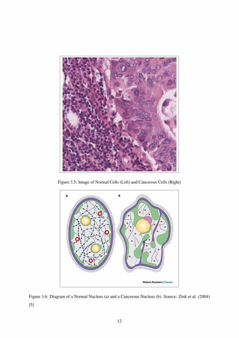
Figure 3.5: Image of Normal Cells (Left) and Cancerous Cells (Right)
Figure 3.6: Diagram of a Normal Nucleus (a) and a Cancerous Nucleus (b). Source: Zink et al. (2004)
[5]
12
symptoms of the high-grade are more apparent at an earlier stage leading to a more effective treatment.
Equally Hodgkin’s lymphoma, whilst being very aggressive, is very treatable. The NHS website [12]
states that:
’Almost 100% of young people with Hodgkin’s lymphoma will achieve a full cure. For older people
over the age of 50, the cure rate is around 75-80%.’
The second situation indicated by cancer in the lymphatic system is a primary cancer growth elsewhere
in the body. In this case the presence of cancerous cells in the lymph node indicates that the cancer has
started to spread throughout the body. This period is crucial in the treatment of the patient. The earlier
the cancer is detected, the more likely it is that the treatment will be successful. The general treatment
for these cancers is chemotherapy.
As stated in section 3.3, the structure of the nucleus is crucial for cancer detection. The difference in
the cellular structure between the cancerous cells and the normal cells is a major distinguishing feature.
This difference is highlighted by the stain applied to the slide. When H&E is applied to the slide the
nuclei are stained purple and the cytoplasm and other tissue is stained pink. Due to the structure of the
cells, a normal region of a lymph node appears almost completely purple. There will also be a small
amount of pink residue present. This is a combination of minimal cytoplasm in the cells and some
excess tissue residue on the slide. This residue can be seen in figure 3.4. In contrast the cancerous cells
are stained a much lighter purple due to the altered structure structure highlighted in section 3.3. As
is visible in figure 3.5 the normal nuclei are a dark purple colour when stained where as the cancerous
cells are a much lighter purple. The other crucial difference to notice is the increased area present
between the nuclei. This is caused by the increased volume of cytoplasm present in the cells. When
the slide is stained, these characteristics lead to the pink concentration of a cancerous region being far
higher than that of a normal section. This is visible in figure 3.5. The normal left hand side has a far
greater concentration of purple colouring than the cancerous right hand side. Equally the number of
nuclei present in an image is another good indicator. Due to the smaller size of the normal cells, the
concentration present is usually far higher. Conversely, the cancerous cells are far larger due to the
mutations and so the concentration of cancerous cells in a given area is far lower than that of normal
cells. Colour was the basis for Patel(2008)[14]. In that project the images were converted to the HSV
image format and the colours present were extracted. These were then matched to the test data to give
results due to the closest match to the data.
Another major characteristic of cancerous growth is the presence of necrosis in a sample. This is
13
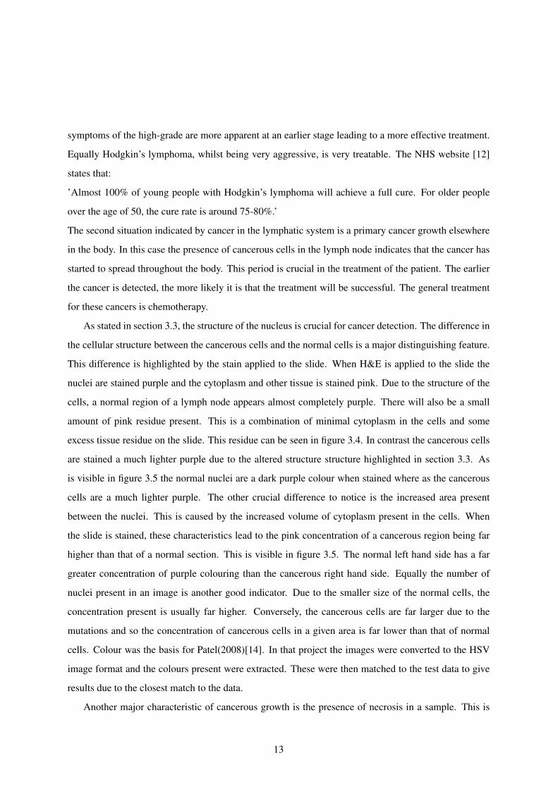
Figure 3.7: Image of a Cancerous Region where Necrosis has developed
the premature death of cells and tissue. Whilst there can be multiple reasons for the development of
necrosis in the node, the major reason is a cancerous growth. In this case, the tumor has outgrown the
blood supply to the area and so cannot obtain enough nutrients to sustain the cellular life present. As
this continues the cells gradually die and begin to break down. However, cells which die in this manner
do not emit the usual signals of a dying cell. This prevents the phagocytes, which engulf and break
down the dead tissue, from locating these cells. This in turn leads to nearby cells becoming poisoned
from the toxins released and increases the cell death in this location. As this continues whole sections of
nodes will die and break down to form these areas of dead tissue. These areas are very apparent on the
slides, as they are stained with a very vibrant pink/red colour and contain no nuclei which eliminates any
purple areas. This is shown in figure 3.7. Unfortunately scar tissue can resemble necrosis quite closely.
The big difference in appearance is that there are nuclei present in the tissue area. These nuclei appear
stretched but usually stain in the same way as the normal non-cancerous circular nuclei. This leads to
dark purple cigar-shaped artifacts appearing in the image. This particular tissue type causes some real
problems with automatic analysis as the quantitative methods normally used to diagnose cancer would
14
generally classify these sections as cancerous tissue.
3.5 Colour Deconvolution
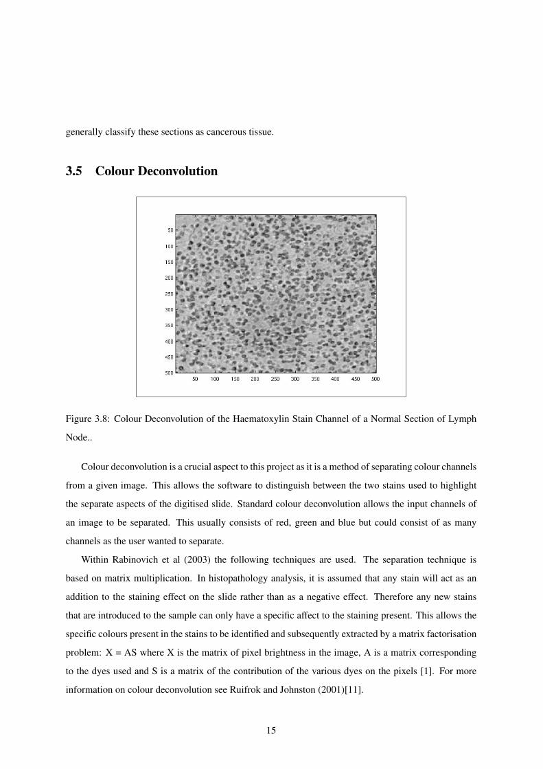
Figure 3.8: Colour Deconvolution of the Haematoxylin Stain Channel of a Normal Section of Lymph
Node..
Colour deconvolution is a crucial aspect to this project as it is a method of separating colour channels
from a given image. This allows the software to distinguish between the two stains used to highlight
the separate aspects of the digitised slide. Standard colour deconvolution allows the input channels of
an image to be separated. This usually consists of red, green and blue but could consist of as many
channels as the user wanted to separate.
Within Rabinovich et al (2003) the following techniques are used. The separation technique is
based on matrix multiplication. In histopathology analysis, it is assumed that any stain will act as an
addition to the staining effect on the slide rather than as a negative effect. Therefore any new stains
that are introduced to the sample can only have a specific affect to the staining present. This allows the
specific colours present in the stains to be identified and subsequently extracted by a matrix factorisation
problem: X = AS where X is the matrix of pixel brightness in the image, A is a matrix corresponding
to the dyes used and S is a matrix of the contribution of the various dyes on the pixels [1]. For more
information on colour deconvolution see Ruifrok and Johnston (2001)[11].
15
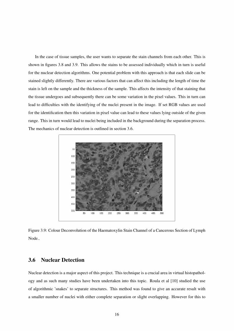
In the case of tissue samples, the user wants to separate the stain channels from each other. This is
shown in figures 3.8 and 3.9. This allows the stains to be assessed individually which in turn is useful
for the nuclear detection algorithms. One potential problem with this approach is that each slide can be
stained slightly differently. There are various factors that can affect this including the length of time the
stain is left on the sample and the thickness of the sample. This affects the intensity of that staining that
the tissue undergoes and subsequently there can be some variation in the pixel values. This in turn can
lead to difficulties with the identifying of the nuclei present in the image. If set RGB values are used
for the identification then this variation in pixel value can lead to these values lying outside of the given
range. This in turn would lead to nuclei being included in the background during the separation process.
The mechanics of nuclear detection is outlined in section 3.6.
Figure 3.9: Colour Deconvolution of the Haematoxylin Stain Channel of a Cancerous Section of Lymph
Node..
3.6 Nuclear Detection
Nuclear detection is a major aspect of this project. This technique is a crucial area in virtual histopathol-
ogy and as such many studies have been undertaken into this topic. Roula et al [10] studied the use
of algorithmic ’snakes’ to separate structures. This method was found to give an accurate result with
a smaller number of nuclei with either complete separation or slight overlapping. However for this to
16
work the algorithm must know the centre points of the nuclei. This can either be done manually with
the user selecting the centres and providing this data to the algorithm or an automatic algorithm can be
used. According to the report, however, ”...the method tends to degrade with large numbers of nuclei”
[10]. This would be a serious limiting factor in this project as the number of nuclei per 500 by 500
pixels section of the slide would reach many hundreds, if not low thousands. The images being used
typically consist of twenty thousand or more pixels per side and so the sheer number of nuclei makes a
manual method totally impractical.
Another approach is edge detection. This is described in detail in Magee (2007) [4]. Edge detection
is generally carried out by checking the gradients between pixels. If a great change exists then it is likely
that an edge exists at this point. This can be carried out throughout the entire image to provide an outline
of all the components present in the image. A higher sensitivity will generally increase the accuracy of
the algorithm, however, if the sensitivity becomes too high then components can be split into more than
one artifact by the algorithm.
Alex Wright’s project in 2006-07 [2] used nuclear detection for cancer detection. The idea behind
his method was using colour deconvolution to produce images with greater gradient changes between
components coupled with an average nuclear size. This approach seems to be the most appropriate
for this project. One limitation of the method is that cancerous nuclei generally have a much greater
diameter than normal nuclei. This can lead to multiple detections of the same nucleus in an image.
However, from the results obtained so far using this method, when the number of double positives are
compared to the number of undetected nuclei, it appears that these are similar enough figures to be
negligible. Equally the percentage of double positives and undetected nuclei is generally below five
percent and so do not seriously affect the results.
3.7 Delaunay Triangulation
Delaunay triangulation uses a series of points and creates the smallest possible triangular mesh from
these points such that no point is within another triangle. The benefit of this method is that it allows the
distances between points to be calculated properly and gives a quantitative value to the distribution. This
technique has been used with some success in other studies including Mulchrone (2002) [9], Keenan et al
(2000) [16] and Swainston (2008) [8]. Mulchrone was actually concerned with strain analysis in geology
rather than cancer detection, however the principal is the same. In Mulchrone the triangulation method
17
was used to good effect in locating the nearest neighbour from strain points. This applies equally to
Keenan et al where it was used to calculate the inter-nuclear distances. Keenan et al were concerned with
cervical dysplasia and the varying differences in the different stages of the dysplasia. The triangulation
was used to calculate how the inter-nuclear distances altered as the dysplasia progressed. It was found
that across the five classes there were significant differences in the average lengths and areas.
3.8 Current Solutions
In the current market, there are no fully automated solutions for the detection of cancer. There have been
multiple studies in this area with most significance being placed on breast cancer due to the screening
program in place. The study of Qi and Head (2004) [7] was concerned with this exact problem; however,
they were using infrared to study the samples. Other studies have been carried out in this field including
Mesker et al. (2003) [17]. This particular study was concerned with analysing lymph tissue for colorec-
tal cancer, as this project is. However, the direction taken by the researchers was very different to the
one outlined in this project. Mesker et al. (2003) used a technique called reverse transcript polymerase
chain reaction (RT-PCR) which uses an enzyme to replicate the RNA present. The object of this study
was to detect an artifact called the carcinoembryonic antigen (CEA) as it had previously been found to
be a reasonable indicator of recurrence in previously cured patients in a study carried out by Liefers et
al. (1998) [6].
Whilst these solutions have been useful in diagnosing cancer in patients, there still exists no com-
plete system. The majority of automatic detection solutions are based on the RNA replication method
outlined in the study of Mesker et al. (2003) [17]. This is very time intensive and requires more human
input than the staining and preparation of slides. A more desirable solution would be one which re-
quired the minimum amount of human interaction possible. This project looks at a less labour intensive
solution.
18
Chapter 4
Design and Implementation
4.1 Research
Due to the different competencies necessary for this project, the research section of the project was cru-
cial in the understanding of the problem. A major component is the biological behaviour of the cells and
the metamorphosis of the nodes when a cancer is developing. The basic understanding of the problem
came from meeting with the pathologist, Darren Treanor. Once the basic principles were understood,
attention then moved to finding papers and journals concerning the development of cancerous growths
in the human body. For this task, the Cancer Research UK (http://www.cancerresearchuk.org/) and the
World Health Organisation (www.WHO.int) were fantastic sources for an overview of cancer behaviour
with particular significance being placed on the WHO’s factsheet [18]. This then lead onto the research
cited in section 3.3 with Zink et al (2004) [5] being a major aid in the understanding of the cell nucleus’
metamorphosis.
The initial task was to split the problem into smaller, more manageable sections. This lead to the
following tasks:
• Image retrieval
19
• Nuclear detection
• Colour analysis
• Diagnosis
4.1.1 Usable Technologies
For this project there were a number of useful methods available. These are discussed below. As this
is area is very experimental, the need for rapid-prototyping was crucial when deciding on the software
and languages to be used.
4.1.1.1 Matlab
This is a very useful piece of software for mathematical calculations. It is a interactive development
environment with its own in-built high-level language. It specialises in the manipulation of matrices,
the plotting of functions and the creation of algorithms. It is commonly used for scientific research and
modelling technical data such as air resistance or fluid mechanics. The major advantage of Matlab is the
ease of which basic algorithms can be developed and therefore, as this project requires rapid prototyping,
Matlab is an ideal solution. The other major strength to Matlab is its connection with scientific research.
This has lead to a vast community developing scripts for the program which in turn can be incorporated
into the software development stage. Another factor is that Matlab has a number of included tools for
working with images. This project relies on the pathological images for its main source of data and as
such, these tools are very useful. Another useful aspect of Matlab is its capability for visualising data, i.e.
creating histograms. As this project is concerned with the quantitative values present in the images, this
particular feature is very useful for comparing data and creating and supporting hypotheses. The final
advantage of Matlab is its ability to incorporate other languages into its own scripts and function files.
For C or FORTRAN this is accomplished by using MEX files. MEX stands for Matlab EXecutable
and is created from the original C or FORTRAN routines and incorporates all the necessary library
sections to allow the functions to be run directly from the Matlab interface. This is useful where a
function already exists in one of these languages and prevents the programmer from having to rewrite
the function in Matlab. One issue with Matlab is that as it is a high-level language the code is not as
efficient for processors as when coded in a lower-level language such as C. This can lead to processor
20
intensive tasks taking longer to run to completion. However it was felt that this factor was outweighed
by the benefits outlined above.
4.1.1.2 C/C++
Other languages commonly used for development of computer vision systems are C and C++. This is
due to the nature of the languages. They are both low-level languages which allow the programmer
to directly control the memory allocation for a particular process. This has lead to C and C++ being
far more efficient in processor intensive routines. However conversely this extra control means that the
implementation of routines take longer as there is more coding necessary. The disadvantage of this is
that this project requires the ability to rapid prototype which is not a strength of either of these languages.
Equally whilst certain useful routines in the computer vision discipline are coded in C or C++ Matlab,
as highlighted previously, has the ability to incorporate these files into its own running.
4.1.1.3 Java and Python
These languages were briefly considered as they are both high-level languages which would allow rapid
prototyping. However, both languages lack the in-built tools that Matlab boasts which allow for fast
analysis of results. This would be a serious hindrance as the benefit of the rapid prototyping would
be massively outweighed by the extra coding necessary to produce the useful figures. In addition the
problems with using any high-level language (code efficiency and memory allocation for example) are
still relevant making these two languages totally inappropriate for this project.
4.1.1.4 OpenCV
This is the Open Source Computer Vision library which consists of methods useful to any development
of a computer vision software package. The majority of the methods included are concerned with real-
time vision. It was originally started by Intel but has since become open source allowing anyone to
use and develop for it. This has led to a large community of users which, like the Matlab community,
support each other in the development of software. It has been mainly coded in C++ and so is very
efficient. It is an attractive solution to be used in tandem with C/C++ and Matlab as the efficiency of the
code together with the functionality of the library can lead to a very powerful solution.
21
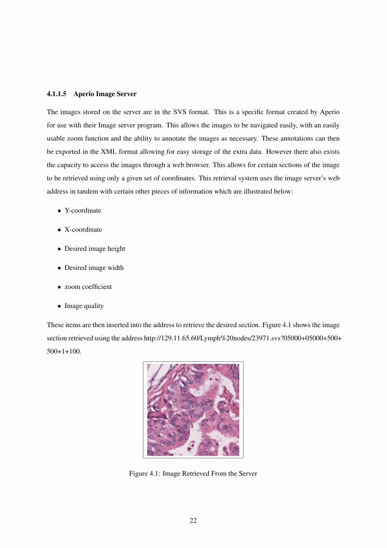
4.1.1.5 Aperio Image Server
The images stored on the server are in the SVS format. This is a specific format created by Aperio
for use with their Image server program. This allows the images to be navigated easily, with an easily
usable zoom function and the ability to annotate the images as necessary. These annotations can then
be exported in the XML format allowing for easy storage of the extra data. However there also exists
the capacity to access the images through a web browser. This allows for certain sections of the image
to be retrieved using only a given set of coordinates. This retrieval system uses the image server’s web
address in tandem with certain other pieces of information which are illustrated below:
• Y-coordinate
• X-coordinate
• Desired image height
• Desired image width
• zoom coefficient
• Image quality
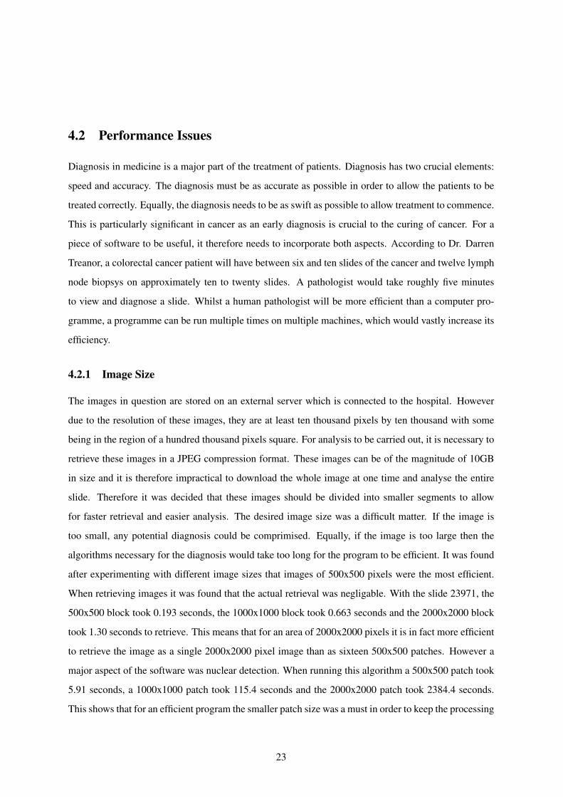
These items are then inserted into the address to retrieve the desired section. Figure 4.1 shows the image
section retrieved using the address http://129.11.65.60/Lymph%20nodes/23971.svs?05000+05000+500+
500+1+100.
Figure 4.1: Image Retrieved From the Server
22
4.2 Performance Issues
Diagnosis in medicine is a major part of the treatment of patients. Diagnosis has two crucial elements:
speed and accuracy. The diagnosis must be as accurate as possible in order to allow the patients to be
treated correctly. Equally, the diagnosis needs to be as swift as possible to allow treatment to commence.
This is particularly significant in cancer as an early diagnosis is crucial to the curing of cancer. For a
piece of software to be useful, it therefore needs to incorporate both aspects. According to Dr. Darren
Treanor, a colorectal cancer patient will have between six and ten slides of the cancer and twelve lymph
node biopsys on approximately ten to twenty slides. A pathologist would take roughly five minutes
to view and diagnose a slide. Whilst a human pathologist will be more efficient than a computer pro-
gramme, a programme can be run multiple times on multiple machines, which would vastly increase its
efficiency.
4.2.1 Image Size
The images in question are stored on an external server which is connected to the hospital. However
due to the resolution of these images, they are at least ten thousand pixels by ten thousand with some
being in the region of a hundred thousand pixels square. For analysis to be carried out, it is necessary to
retrieve these images in a JPEG compression format. These images can be of the magnitude of 10GB
in size and it is therefore impractical to download the whole image at one time and analyse the entire
slide. Therefore it was decided that these images should be divided into smaller segments to allow
for faster retrieval and easier analysis. The desired image size was a difficult matter. If the image is
too small, any potential diagnosis could be comprimised. Equally, if the image is too large then the
algorithms necessary for the diagnosis would take too long for the program to be efficient. It was found
after experimenting with different image sizes that images of 500x500 pixels were the most efficient.
When retrieving images it was found that the actual retrieval was negligable. With the slide 23971, the
500x500 block took 0.193 seconds, the 1000x1000 block took 0.663 seconds and the 2000x2000 block
took 1.30 seconds to retrieve. This means that for an area of 2000x2000 pixels it is in fact more efficient
to retrieve the image as a single 2000x2000 pixel image than as sixteen 500x500 patches. However a
major aspect of the software was nuclear detection. When running this algorithm a 500x500 patch took
5.91 seconds, a 1000x1000 patch took 115.4 seconds and the 2000x2000 patch took 2384.4 seconds.
This shows that for an efficient program the smaller patch size was a must in order to keep the processing
23
time down. Due to this the 500x500 pixel patch was deemed to be the best comprimise.
One issue of the image retrieval is the network latency. On occasions there can be issues with
the network which slow down the retrieval. One idea to combat this would be to retrieve the patches
prior to the analysis and store them locally. However as outlined previously these images can be over
20,000x20,000 pixels leading to a large amount of storage being required to store these patches. Using
the patch size outlined above, an average node consists of roughly 600 patches. Using the JPEG format
these will usually take up 30MB per node. As some slides can consist of six nodes this would soon
increase to a large amount of space necessary to store such files. The other issue to this is that these
images contain sensitive patient information. Duplicating the data increases the chance of the patients’
confidentiality being compromised.
4.3 Proposed Resources
After much deliberation it was decided that the best solution for the development of this project would
be to use Matlab in conjunction with some smaller C++ files and the OpenCV library. For the retrieval
of the images a combination of the Aperio image server and the web retrieval method would be used.
The Aperio image server would allow for the images to be annotated and viewed at multiple zooms to
give a better overview of the slide diagnosis whilst the web retrieval method would allow smaller, more
efficient images to be retrieved and analysed. It was felt that the advantages of Matlab outweighed its
disadvantages. Whilst C/C++ and OpenCV is generally more efficient the extra time taken to code the
software would be a serious disadvantage for the multiple prototypes necessary for this project. There
were multiple hardware configurations to be used for this project. There were two platforms on which
this program was developed, Windows and Linux. The machines in the University’s labs are Linux
based with 4GB of RAM and an Intel Core2Quad processor with each core running at 2.50GHz. The
main Windows machine has an Intel Core2 Duo process running at 2.0GHz and 3GB of RAM whilst the
Citrix based server runs an Intel Xeon processor running at 2.8GHz with 4GB of RAM. It was hoped
that the project would be fully compatible on both platforms. As the code has mainly been written in
Matlab this would hopefully accomplish this.
24
4.4 Image Retrieval
Whilst Aperio Image Server is a very useful program for viewing the slide images, unfortunately the
quality of the JPEG files that can be produced using the built-in snapshot function is not high enough
for some of the algorithms to run properly. Therefore the image patches needed to be retrieved using the
http retrieval method outlined previously as the quality of the image patches retrieved can then be stated,
allowing for better quality images and the best chance of the algorithm detecting any cancer present in
the patches.
There were two options for this method. One was to retrieve the patches prior to testing and store the
images on the hard drive as JPEG files. This method was to be used for testing outside of the University’s
systems where the internet connection might be the limiting factor. The other was to retrieve each patch
individually, store it in the computer’s RAM, test it and then replace it with the next patch. This was seen
as a more efficient way to conduct the testing from within the University. This method saved storage
space and was seen as a more resource friendly method than the former. However, it was decided
that both methods would be useful for different scenarios and so both were developed. Both methods
retrieved the patches in images of 500x500 pixels.
4.5 Node Extraction
A serious issue with this project is that slides may contain more than one node. Therefore the amount
of background present on these slides will increase as the number of nodes increase. To reduce the
computation time necessary to process a slide, it was decided that identifying and extracting only the
image patches pertinent to the node would be preferential to retrieving the entire image. There were
two parts to this task: firstly, identify the nodes in an image and secondly, calculate the relevant image
coordinates in order to retrieve the desired sections.
The first task was solved using connected components analysis. The method was to convert a slide
image retrieved at a 40th of its actual size to allow the entire slide to be captured in a single image.
This image was then processed to invert the colours and create a negative image. A method called
brightnessthreshold was then applied to the inverted image. This method produces a binary mask of the
image where the pixel brightness is above a given level. This was found to be very effective at removing
the background as this section was mainly white or off-white and so, in a negative image, lay beneath
the threshold. This mask then had a gaussian filter applied to it to smooth out the image. Figure 4.2
25
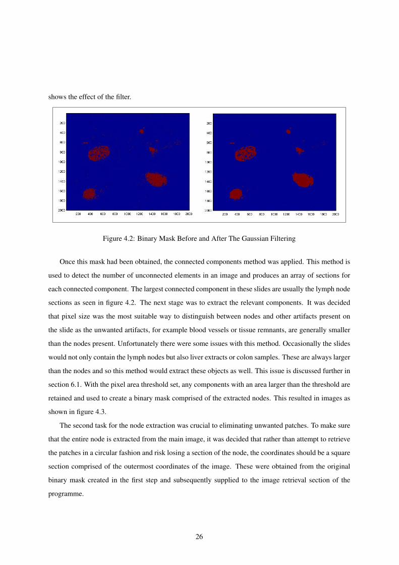
shows the effect of the filter.
Figure 4.2: Binary Mask Before and After The Gaussian Filtering
Once this mask had been obtained, the connected components method was applied. This method is
used to detect the number of unconnected elements in an image and produces an array of sections for
each connected component. The largest connected component in these slides are usually the lymph node
sections as seen in figure 4.2. The next stage was to extract the relevant components. It was decided
that pixel size was the most suitable way to distinguish between nodes and other artifacts present on
the slide as the unwanted artifacts, for example blood vessels or tissue remnants, are generally smaller
than the nodes present. Unfortunately there were some issues with this method. Occasionally the slides
would not only contain the lymph nodes but also liver extracts or colon samples. These are always larger
than the nodes and so this method would extract these objects as well. This issue is discussed further in
section 6.1. With the pixel area threshold set, any components with an area larger than the threshold are
retained and used to create a binary mask comprised of the extracted nodes. This resulted in images as
shown in figure 4.3.
The second task for the node extraction was crucial to eliminating unwanted patches. To make sure
that the entire node is extracted from the main image, it was decided that rather than attempt to retrieve
the patches in a circular fashion and risk losing a section of the node, the coordinates should be a square
section comprised of the outermost coordinates of the image. These were obtained from the original
binary mask created in the first step and subsequently supplied to the image retrieval section of the
programme.
26
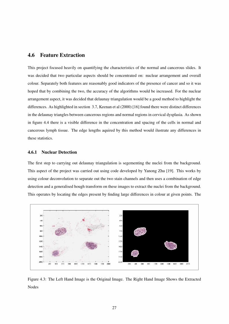
4.6 Feature Extraction
This project focused heavily on quantifying the characteristics of the normal and cancerous slides. It
was decided that two particular aspects should be concentrated on: nuclear arrangement and overall
colour. Separately both features are reasonably good indicators of the presence of cancer and so it was
hoped that by combining the two, the accuracy of the algorithms would be increased. For the nuclear
arrangement aspect, it was decided that delaunay triangulation would be a good method to highlight the
differences. As highlighted in section 3.7, Keenan et al (2000) [16] found there were distinct differences
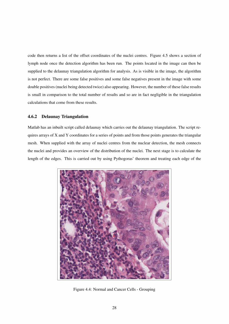
in the delaunay triangles between cancerous regions and normal regions in cervical dysplasia. As shown
in figure 4.4 there is a visible difference in the concentration and spacing of the cells in normal and
cancerous lymph tissue. The edge lengths aquired by this method would ilustrate any differences in
these statistics.
4.6.1 Nuclear Detection
The first step to carrying out delaunay triangulation is segementing the nuclei from the background.
This aspect of the project was carried out using code developed by Yanong Zhu [19]. This works by
using colour deconvolution to separate out the two stain channels and then uses a combination of edge
detection and a generalised hough transform on these images to extract the nuclei from the background.
This operates by locating the edges present by finding large differences in colour at given points. The
Figure 4.3: The Left Hand Image is the Original Image. The Right Hand Image Shows the Extracted
Nodes
27
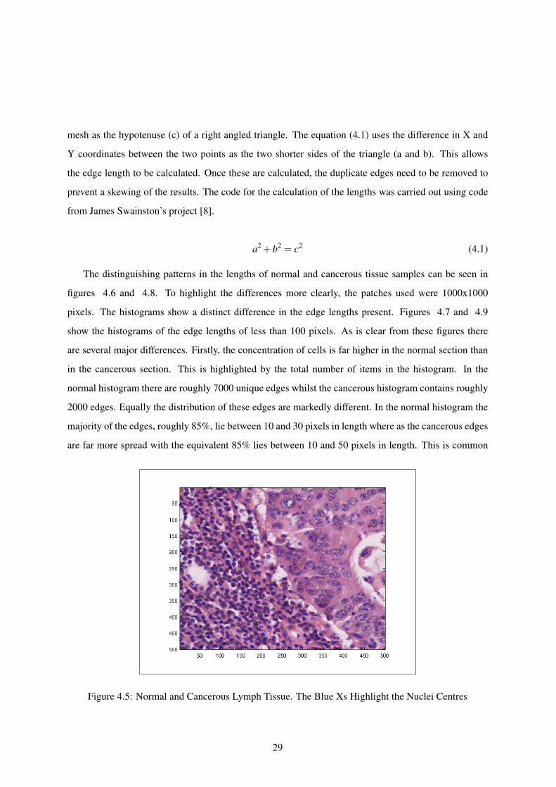
code then returns a list of the offset coordinates of the nuclei centres. Figure 4.5 shows a section of
lymph node once the detection algorithm has been run. The points located in the image can then be
supplied to the delaunay triangulation algorithm for analysis. As is visible in the image, the algorithm
is not perfect. There are some false positives and some false negatives present in the image with some
double positives (nuclei being detected twice) also appearing. However, the number of these false results
is small in comparison to the total number of results and so are in fact negligible in the triangulation
calculations that come from these results.
4.6.2 Delaunay Triangulation
Matlab has an inbuilt script called delaunay which carries out the delaunay triangulation. The script re-
quires arrays of X and Y coordinates for a series of points and from those points generates the triangular
mesh. When supplied with the array of nuclei centres from the nuclear detection, the mesh connects
the nuclei and provides an overview of the distribution of the nuclei. The next stage is to calculate the
length of the edges. This is carried out by using Pythogoras’ theorem and treating each edge of the
Figure 4.4: Normal and Cancer Cells - Grouping
28
mesh as the hypotenuse (c) of a right angled triangle. The equation (4.1) uses the difference in X and
Y coordinates between the two points as the two shorter sides of the triangle (a and b). This allows
the edge length to be calculated. Once these are calculated, the duplicate edges need to be removed to
prevent a skewing of the results. The code for the calculation of the lengths was carried out using code
from James Swainston’s project [8].
a2 +b2 = c2 (4.1)
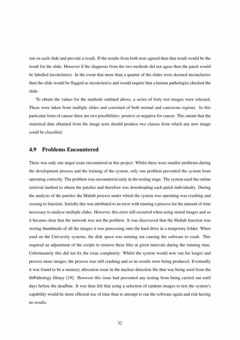
The distinguishing patterns in the lengths of normal and cancerous tissue samples can be seen in
figures 4.6 and 4.8. To highlight the differences more clearly, the patches used were 1000x1000
pixels. The histograms show a distinct difference in the edge lengths present. Figures 4.7 and 4.9
show the histograms of the edge lengths of less than 100 pixels. As is clear from these figures there
are several major differences. Firstly, the concentration of cells is far higher in the normal section than
in the cancerous section. This is highlighted by the total number of items in the histogram. In the
normal histogram there are roughly 7000 unique edges whilst the cancerous histogram contains roughly
2000 edges. Equally the distribution of these edges are markedly different. In the normal histogram the
majority of the edges, roughly 85%, lie between 10 and 30 pixels in length where as the cancerous edges
are far more spread with the equivalent 85% lies between 10 and 50 pixels in length. This is common
Figure 4.5: Normal and Cancerous Lymph Tissue. The Blue Xs Highlight the Nuclei Centres
29
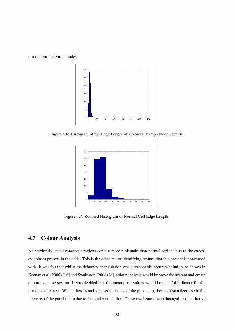
throughout the lymph nodes.
Figure 4.6: Histogram of the Edge Length of a Normal Lymph Node Section.
Figure 4.7: Zoomed Histogram of Normal Cell Edge Length.
4.7 Colour Analysis
As previously stated cancerous regions contain more pink stain than normal regions due to the excess
cytoplasm present in the cells. This is the other major identifying feature that this project is concerned
with. It was felt that whilst the delaunay triangulation was a reasonably accurate solution, as shown in
Keenan et al (2000) [16] and Swainston (2008) [8], colour analysis would improve the system and create
a more accurate system. It was decided that the mean pixel values would be a useful indicator for the
presence of cancer. Whilst there is an increased presence of the pink stain, there is also a decrease in the
intensity of the purple stain due to the nuclear mutation. These two issues mean that again a quantitative
30
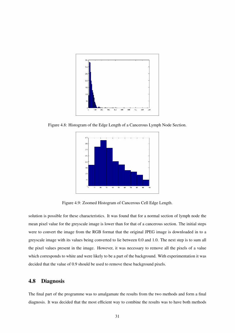
Figure 4.8: Histogram of the Edge Length of a Cancerous Lymph Node Section.
Figure 4.9: Zoomed Histogram of Cancerous Cell Edge Length.
solution is possible for these characteristics. It was found that for a normal section of lymph node the
mean pixel value for the greyscale image is lower than for that of a cancerous section. The initial steps
were to convert the image from the RGB format that the original JPEG image is downloaded in to a
greyscale image with its values being converted to lie between 0.0 and 1.0. The next step is to sum all
the pixel values present in the image. However, it was necessary to remove all the pixels of a value
which corresponds to white and were likely to be a part of the background. With experimentation it was
decided that the value of 0.9 should be used to remove these background pixels.
4.8 Diagnosis
The final part of the programme was to amalgamate the results from the two methods and form a final
diagnosis. It was decided that the most efficient way to combine the results was to have both methods
31
run on each slide and provide a result. If the results from both tests agreed then that result would be the
result for the slide. However if the diagnosis from the two methods did not agree then the patch would
be labelled inconclusive. In the event that more than a quarter of the slides were deemed inconclusive
then the slide would be flagged as inconclusive and would require that a human pathologist checked the
slide.
To obtain the values for the methods outlined above, a series of forty test images were selected.
These were taken from multiple slides and consisted of both normal and cancerous regions. In this
particular form of cancer there are two possibilities: positive or negative for cancer. This meant that the
statistical data obtained from the image tests should produce two classes from which any new image
could be classified.
4.9 Problems Encountered
There was only one major issue encountered in this project. Whilst there were smaller problems during
the development process and the training of the system, only one problem prevented the system from
operating correctly. The problem was encountered early in the testing stage. The system used the online
retrieval method to obtain the patches and therefore was downloading each patch individually. During
the analysis of the patches the Matlab process under which the system was operating was crashing and
ceasing to function. Initially this was attributed to an error with running a process for the amount of time
necessary to analyse multiple slides. However, this error still occurred when using stored images and so
it became clear that the network was not the problem. It was discovered that the Matlab function was
storing thumbnails of all the images it was processing onto the hard drive in a temporary folder. When
used on the University systems, the disk space was running out causing the software to crash. This
required an adjustment of the scripts to remove these files at given intervals during the running time.
Unfortunately this did not fix the issue completely. Whilst the system would now run for longer and
process more images, the process was still crashing and so no results were being produced. Eventually
it was found to be a memory allocation issue in the nuclear detection file that was being used from the
libPathology library [19]. However this issue had prevented any testing from being carried out until
days before the deadline. It was then felt that using a selection of random images to test the system’s
capability would be more efficient use of time than to attempt to run the software again and risk having
no results.
32
Chapter 5
Results Analysis
5.1 Programme Results
The programme was tested using eighty images extracted from the server from multiple slides. These
were divided into normal and cancerous images with forty of each. These images included sections of
cancerous cells, necrosis, scar tissue and images of residual tissue instead of lymph node. This was in
order to fully test the capability of the system. The system was then tested on these images to give an
overall accuracy of the software. The potential classifications given were:
• Normal - no cancer detected in the image.
• Cancer - cancerous cells detected in the image.
• Cancer with the potential for the presence of necrosis - cancerous cells and/or necrosis detected
in the image.
• Inconclusive - the two methods have not agreed in their diagnosis.
It was felt that a conservative solution would be more appropriate for a system of this kind as an incor-
rect diagnosis is potentially far more harmful to the patient than an inconclusive diagnosis. This would
prompt the pathologist to check the slide and manually diagnose the patient. Table 5.1 show the results
33
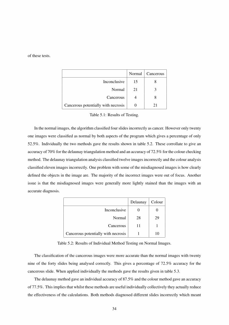
of these tests.
Normal Cancerous
Inconclusive 15 8
Normal 21 3
Cancerous 4 8
Cancerous potentially with necrosis 0 21
Table 5.1: Results of Testing.
In the normal images, the algorithm classified four slides incorrectly as cancer. However only twenty
one images were classified as normal by both aspects of the program which gives a percentage of only
52.5%. Individually the two methods gave the results shown in table 5.2. These corrollate to give an
accuracy of 70% for the delaunay triangulation method and an accuracy of 72.5% for the colour checking
method. The delaunay triangulation analysis classified twelve images incorrectly and the colour analysis
classified eleven images incorrectly. One problem with some of the misdiagnosed images is how clearly
defined the objects in the image are. The majority of the incorrect images were out of focus. Another
issue is that the misdiagnosed images were generally more lightly stained than the images with an
accurate diagnosis.
Delaunay Colour
Inconclusive 0 0
Normal 28 29
Cancerous 11 1
Cancerous potentially with necrosis 1 10
Table 5.2: Results of Individual Method Testing on Normal Images.
The classification of the cancerous images were more accurate than the normal images with twenty
nine of the forty slides being analysed correctly. This gives a percentage of 72.5% accuracy for the
cancerous slide. When applied individually the methods gave the results given in table 5.3.
The delaunay method gave an individual accuracy of 87.5% and the colour method gave an accuracy
of 77.5%. This implies that whilst these methods are useful individually collectively they actually reduce
the effectiveness of the calculations. Both methods diagnosed different slides incorrectly which meant
34
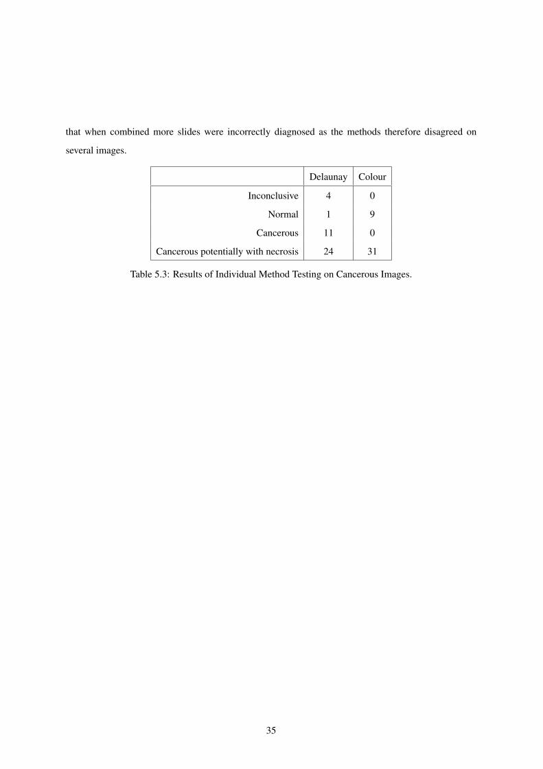
that when combined more slides were incorrectly diagnosed as the methods therefore disagreed on
several images.
Delaunay Colour
Inconclusive 4 0
Normal 1 9
Cancerous 11 0
Cancerous potentially with necrosis 24 31
Table 5.3: Results of Individual Method Testing on Cancerous Images.
35
Chapter 6
Evaluation
6.1 Image Retrieval
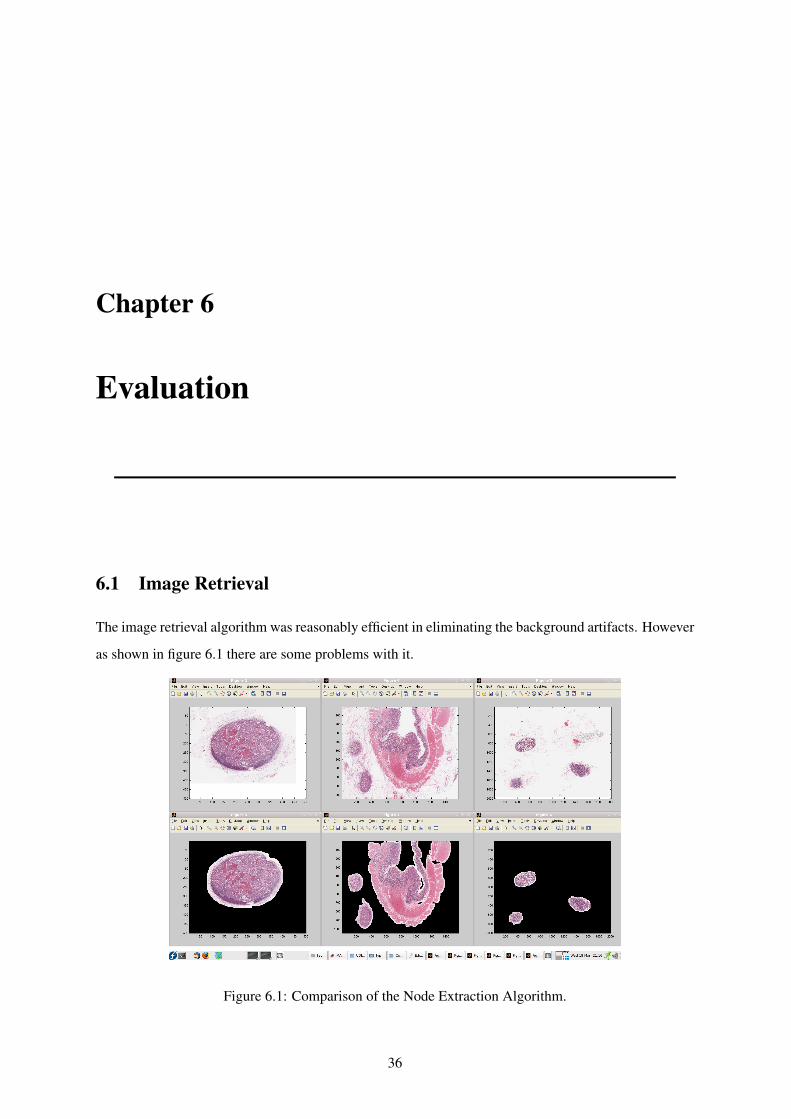
The image retrieval algorithm was reasonably efficient in eliminating the background artifacts. However
as shown in figure 6.1 there are some problems with it.
Figure 6.1: Comparison of the Node Extraction Algorithm.
36
As the algorithm relies on pixel area for identifying the nodes, certain other artifacts present on the
slide can be extracted as well. For instance in the second slide, the nodes are in the bottom left corner
but a section of colon is also present on the slide. As the pixel area of the colon section is far larger than
the area size threshold it is also extracted. When run on this image the algorithm finds four nodes rather
than two as the top right hand side of the sample is not actually connected to the rest of the sample and
so is treated as a separate component. One idea to remove the incorrect objects from the image was to
analyse the shape of the objects. As is visible in figure 6.1 the nodes are generally circular in shape.
The idea was to find the centroid of the component and then check the distances to the edges. If these
distances were found to be roughly the same or tending towards two different lengths the artifact was
likely to be a node. This technique should eliminate the excess tissue present.
There are three issues with this. Firstly, some of the unwanted artifacts present are circular. This is
visible in figure 6.1 in the middle images. The top right hand side of the slide has a circular structure
which is roughly the same size as a lymph node and is also circular. the previously stated method would
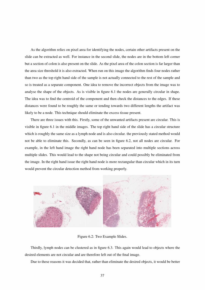
not be able to eliminate this. Secondly, as can be seen in figure 6.2, not all nodes are circular. For
example, in the left hand image the right hand node has been separated into multiple sections across
multiple slides. This would lead to the shape not being circular and could possibly be eliminated from
the image. In the right hand issue the right hand node is more rectangular than circular which in its turn
would prevent the circular detection method from working properly.
Figure 6.2: Two Example Slides.
Thirdly, lymph nodes can be clustered as in figure 6.3. This again would lead to objects where the
desired elements are not circular and are therefore left out of the final image.
Due to these reasons it was decided that, rather than eliminate the desired objects, it would be better
37
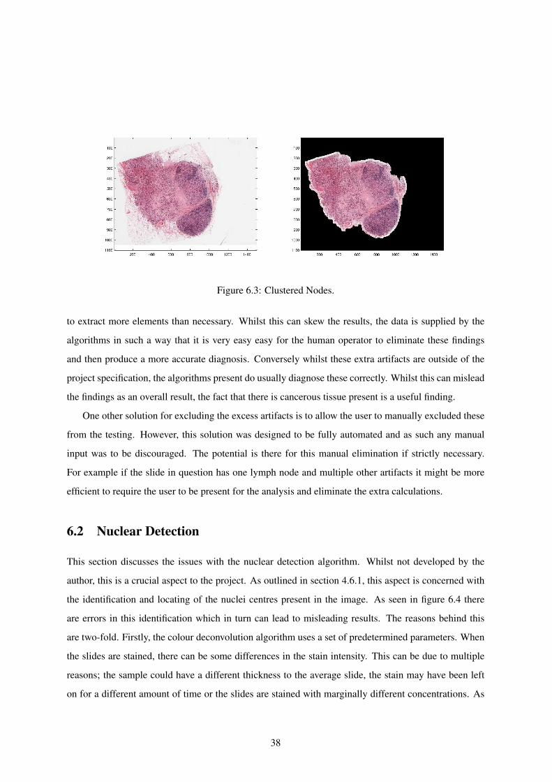
Figure 6.3: Clustered Nodes.
to extract more elements than necessary. Whilst this can skew the results, the data is supplied by the
algorithms in such a way that it is very easy easy for the human operator to eliminate these findings
and then produce a more accurate diagnosis. Conversely whilst these extra artifacts are outside of the
project specification, the algorithms present do usually diagnose these correctly. Whilst this can mislead
the findings as an overall result, the fact that there is cancerous tissue present is a useful finding.
One other solution for excluding the excess artifacts is to allow the user to manually excluded these
from the testing. However, this solution was designed to be fully automated and as such any manual
input was to be discouraged. The potential is there for this manual elimination if strictly necessary.
For example if the slide in question has one lymph node and multiple other artifacts it might be more
efficient to require the user to be present for the analysis and eliminate the extra calculations.
6.2 Nuclear Detection
This section discusses the issues with the nuclear detection algorithm. Whilst not developed by the
author, this is a crucial aspect to the project. As outlined in section 4.6.1, this aspect is concerned with
the identification and locating of the nuclei centres present in the image. As seen in figure 6.4 there
are errors in this identification which in turn can lead to misleading results. The reasons behind this
are two-fold. Firstly, the colour deconvolution algorithm uses a set of predetermined parameters. When
the slides are stained, there can be some differences in the stain intensity. This can be due to multiple
reasons; the sample could have a different thickness to the average slide, the stain may have been left
on for a different amount of time or the slides are stained with marginally different concentrations. As
38
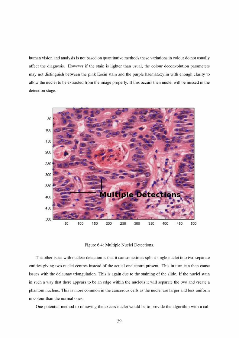
human vision and analysis is not based on quantitative methods these variations in colour do not usually
affect the diagnosis. However if the stain is lighter than usual, the colour deconvolution parameters
may not distinguish between the pink Eosin stain and the purple haematoxylin with enough clarity to
allow the nuclei to be extracted from the image properly. If this occurs then nuclei will be missed in the
detection stage.
Figure 6.4: Multiple Nuclei Detections.
The other issue with nuclear detection is that it can sometimes split a single nuclei into two separate
entities giving two nuclei centres instead of the actual one centre present. This in turn can then cause
issues with the delaunay triangulation. This is again due to the staining of the slide. If the nuclei stain
in such a way that there appears to be an edge within the nucleus it will separate the two and create a
phantom nucleus. This is more common in the cancerous cells as the nuclei are larger and less uniform
in colour than the normal ones.
One potential method to removing the excess nuclei would be to provide the algorithm with a cal-
39
culation of the possible amount of nuclei in a given area. However this may not solve the issue. The
majority of the duplication errors occur in the cancerous region and the cancerous nuclei are generally
at least twice the diameter of the normal nuclei. With this in mind, the number of potential dual nuclei
detections would likely not exceed the number of normal nuclei in the same area. However, despite
these issues the algorithm is reasonably accurate in detecting the nuclei. On an average slide roughly
3-5% of the total number of nuclei detected will be false positive. Equally the number missed is usually
in this region as well. Overall this should not affect the results of the cancer detection.
6.3 Delaunay Triangulation
The delaunay triangulation was a very useful diagnostic tool. The arrangement of the nuclei is a reason-
able diagnostic process and triangulation is a perfect way to exploit this characteristic. As highlighted
in section 4.6.1, this process is very reliant on the nuclear detection aspect of the system. When there
are errors in the detection, errors begin to appear in the triangulation analysis. This can be seen in figure
4.9. When compared to figure 4.7, the first column (0-10 pixels) is roughly identical in both normal and
cancerous sections. However what is clear from the sample images of these sections is that the closest
nuclei are present in the normal sections and not in the cancerous sections. This can be attributed to the
phantom points created by the nuclei detection. This is an issue as it can skew the statistical analysis
which is applied to the results generated by this method. One method to reduce these errors would be to
exclude any edges under ten pixels. However, this could cause an issue in normal sections as some very
crowded sections can have internuclear distances of less than ten pixels. If these were removed then the
results would not give an accurate portrayal of the image.
6.4 Colour Analysis
The colour analysis method is equally useful. Colour is a major aspect of the diagnostic process and
can be quantified easily. This provides a useful diagnostic tool for an automated system. As seen in
the results this method is 75% accurate in diagnosing images. There were some errors in the analysis
provided for the method. As highlighted previously, the intensity of the staining of the slide is crucial to
this method’s accuracy. If the staining is too light, the mean colour value across the slide will be higher
than the mean value of a more heavily stained slide. This is an issue when analysing slides stained
on different days as the staining process will change subtly from day to day. These difficulties were
40
discussed in section 6.2.
Two possible ways to accommodate this fluctuation are firstly, to convert the image to the HSV
colour format as opposed to the RGB format and secondly, to adjust the colour vectors per batch of
slides. In a usual batch all of the slides will have been sliced and stained in an identical manner and
so should all consist of the same colour intensity. The advantage of the HSV format is that the three
channels do not correspond to different colours. The three channels are hue, saturation and value.
To eliminate the variation the value channel could be ignored. This should remove the most drastic
fluctuations from the analysis and could improve the nuclear detection algorithm as well as the colour
analysis. This method was discussed in Swainston (2008) [8] where graphs were provided to give
examples of the advantages of using this method. Altering the colour vectors per batch should eliminate
the fluctuations completely. However this would make the algorithm less automatic as it would require
configuring before a set of images could be analysed. One option would be to allow the user the choice
of running the fully automated system or providing extra details when deemed necessary.
6.5 System Evaluation
Overall, the system behaved favourably. As shown in the results section the system had an overall
accuracy of 62.5%. With regard to the cancerous cells, this accuracy increased to 72.5% which is
much more appealing. There is also an argument that false positives are more desirable than false
negatives. There are less dire consequences from a false positive that, on further inspection, is found
to be negative than with a false negative that is later found to be positive. One aspect of the system
is that whilst pathologists only agree around about 85% of the time, this system is being compared
to one pathologists results. There could be some inaccuracies present in the perceived results and so
the program could obtain a different result to one pathologist but agree with another. In this research
area an accuracy of over 80% is the desired benchmark. With a few improvements, this project could
conceivably reach this desired benchmark. These further improvements are outlined below.
6.6 Future Improvements
This section discusses some potential enhancements which could be carried out to improve the system’s
accuracy and overall usability. Two major areas were identified; machine learning and extra features.
41
6.6.1 Machine Learning
In the current solution the diagnostic benchmarks are hard coded into the programme files. However,
there may be a case for using a more sophisticated machine learning system to locate further patterns in
the data. Currently the system uses static benchmarks for associating images with the diagnostic classes.
A support vector machine could be used to find new patterns in the results and improve the accuracy of
the system. The SVMs work by treating the input data as a set of vectors and then creating a hyperplane,
for example a line in 2-D space or a plane in 3-D space, which separates the data into two distinct sets.
The hyperplane is then adjusted until the distances to its nearest data points are at a maximum. This
would allow better classification to be provided using the current distinguishing features.
6.6.2 Extra Features
Whilst the internuclear distances and colour are major distinguishing features for detecting cancer in the
lymph nodes, there are many other features that could be used to diagnose cancer. These include:
• Nuclear size and shape - As highlighted in section 3.3 the cancerous nuclei swell and deform.
This is another good diagnostic tool. These cancerous nuclei generally grow to around twice the
size of a normal cell nuclei and so the ability to analyse the images for these enlarged nuclei
would help to diagnose cancerous sections. Equally analysing the shape of these nuclei would
also help in this diagnosis. As the nucleus distorts it loses its circular structure and becomes more
oval shaped. Furthermore this method would be perfect to diagnose scar tissue as the overall area
of the nucleus remains roughly the same as normal nuclei but the shape distorts to a distinct cigar
shape. If this was detectable it could drastically improve the accuracy of the system.
• Colour along the delaunay triangulation lines - This would allow the system to allow for tears
in the tissue, fat deposits or blood vessels in between nuclei. The majority of the colour along a
line between two normal nuclei centres would be purple where as the line between two cancerous
nuclei would generally consist of a lighter purple and pink. This could also be used to analyse
the colour of the immediate area around the centre of the nucleus. In a normal nucleus this will
be a very dark purple where as in a cancerous nucleus this would be a lighter purple with some
hints of pink. This would provide another feature to be analysed when attempting to diagnose the
images.
42
• Tissue texture - No research was carried out into the development of a texture based software
analysis tool. This aspect was briefly looked at in this project research but it was felt that the
nuclear detection and colour analysis was the preferred direction. This area is another major area
for future research in this topic. A combination of the current analysis tools combined with texture
based observations should again increase the accuracy of the system. One such study was carried
out by Hamilton et al. (1997) [13].
With these extra features implemented, the system could then use a voting system to diagnose the
images. If the methods did not provide the same result for an image they could provide a vote and
then the answer with the most votes could then be used. This could then remove the majority of the
inconclusive results from the testing.
6.7 Conclusion
The system developed was reasonably accurate although the overall accuracy was not as high as had
been hoped. However these aspects have been addresses in this report and can hopefully provide the
basis for a more effective system in the future. This research area is a fascinating field; the capacity
for development is vast and could one day completely change the discipline of pathology. This project
has shown that there is enormous potential for a fully automated diagnostic system for cancer to be
developed. In order for this system to be realised, new techniques for identifying the characteristics of
cancer using computer vision must be developed. These methods would then allow the system to better
classify the various types of tissue samples present in the images.
43
Bibliography
[1] A. Rabinovich, S. Agarwal, C.A. Laris, J.H. Price, and S. Belongie. Unsupervised color decom-
position of histologically stained tissue samples. Archives of Pathology and Laboratory Medicine,
2003.
[2] A Wright. The Automated Counting of Cancer Cells Using Computer Vision. Technical report,
University of Leeds, 2007.
[3] C Demir and B Yener. Automated cancer diagnosis based on histopathological images:a systematic
survey. Technical report, 2005.
[4] D Magee. AI31: Computer Vision Notes. University of Leeds, 2007.
[5] D Zink, AH Fischer and JA Nickerson. Nuclear structure in cancer cells. Nature Reviews Cancer,
4(9):677–687, 2004.
[6] G-J Liefers, A-M Cleton-Jansen, CJH van de Velde, J Hermans, JHJM van Krieken, CJ Cornelisse,
and RAEM Tollenaar. Micrometastases and Survival in Stage II Colorectal Cancer. The New
England Journal of Medicine, 339(4):223–228, July 1998.
[7] H Qi and JF Head. Assymetric Analysis Using Automatic Segmentation and Classification for
Breast Cancer Detection in Thermograms. 2004.
[8] J Swainston. A Computer Vision System for the Detection of Cancer in Barretts Oesophagus.
Technical report, University of Leeds, 2008.
[9] KF Mulchrone. Application of Delaunay triangulation to the nearest neighbour method of strain
analysis. Technical report, 2002.
44
[10] MA Roula, A Bouridune and F Kurugollu. An Evolutionary Snake Algorithm for the Segmen-
tation of Nuclei in Histopathological Images. Proceedings of International Conference on Image
Processing 2004, 1:127–130, 2004.
[11] MA Ruifrok, DA Johnston. Quantification of histochemical staining by color deconvolution. Anal
Quant Cytol Histol, 23:291–299, 2001.
[12] NHS Choices. Lymphoma - Introduction.
Accessible at http://www.nhs.uk/Conditions/Lymphoma/pages/Introduction.aspx.
Accessed on 20/04/2009.
[13] PW Hamilton, PH Bartels, D Thompson, NH Anderson, R Montrioni and JM Sloan. Automated
Location of Dysplastic Fields in Colorectal Histology Using Image Texture Analysis. The Journal
of Pathology, 182:68–75, 1997.
[14] R Patel. A Computer Vision Based Approach for Detecting Cancer Cells in Lymph Nodes. Tech-
nical report, University of Leeds, 2008.
[15] S Claydon. Animal Cells, 2006.
Image available at http://scienceaid.co.uk/biology/humans/cells.html, accessed on 01/12/2008.
[16] SJ Keenan, J Diamond, WG McCluggage, H Bharucha, D Thompson, PH Bartels and PW Hamil-
ton. An automated machine vision system for the histological grading of cervical intraepithelial
neoplasia. The Journal of Pathology, 192:351 –362, 2000.
[17] WE Mesker, FS Doekhie, H Vrolijk, R Keyzer, WCR Sloos, H Morreau, PS O’Kelly, GH de
Bock, RAEM Tollenaar and HJ Tanke. Automated Analysis of Multiple Sections for the Detection
of Occult Cells in Lymph Nodes. Clinical Cancer Research, 9:4826 4834, October 2003.
[18] World Health Organisation. Cancer, 2009.
Accessible at http://www.who.int/mediacentre/factsheets/fs297/en/index.html.
Accessed on 20/04/2009.
[19] Y Zhu and D Magee. libpathology library. Code utilised in the project.
45

Appendix A
Personal Reflection
I have enjoyed this project immensely.The topic had some fascinating aspects to it, not least of all, the
biological research that was required. Furthermore this particular research area is very cutting edge and
as such can be very complicated in areas. This suited me perfectly as I have always worked best with
the more complicated and challenging aspects of learning. It was clear form the beginning that this
project was going to be a difficult task to solve and the meetings with Dr. Darren Treanor did nothing to
discourage this view!
The field of pathology was a relatively unknown one to myself. Whilst my family do have a back-
ground in medicine and I, myself nearly chose to study medicine, the majority of the techniques and
terms used when studying this type of discipline were new to me. The research into the biological im-
pact of these cancerous growths was enthralling and kept me interested from the start to the finish of the
project.
The most important thing that this project has taught me is the importance of time management.
This academic year has been very busy with courseworks, this project and my acting being very time
consuming. Due to this it was imperative that a rigorous schedule was adhered to. However, in hindsight
my original schedule was probably not a realistic one. I would have been better served to have began
the design and implementation stage whilst the background research was being carried out. This would
have meant that the research would have had to have been more tightly structured as well. During the
46
research section, I was reading papers on multiple different aspects almost simultaneously. I might
have been been better served to have concentrated on a particular topic in order to have been able to
begin designing the relevant parts of the system whilst still relatively early in the first semester. I would
recommend that future students attempt to structure their workload in this way to fully take advantage
of the first semester.
One minor problem with this project was that the module concerned with computer vision was
taught in the second semester. This meant that certain useful techniques were missed when attempting to
design the system as I was unaware of either their existence or their relevance to this project. For future
students I would recommend reading, in a reasonable amount of detail, the computer vision course notes
and familiarising themselves with the basic methods of image processing and analysis. Furthermore,
whilst I felt reasonably comfortable using Matlab, there was a vast amount of useful techniques included
in the software that I had never experienced before. More general experimentations with Matlab may
have benefited me more than the specific experimentation that I carried out.
My final piece of advice to any student looking to undertake a project is to pick a topic that you
are interested in. That is the most important aspect of the project as the innate interest is what will give
you the motivation to continue when all you feel like doing is going and lying in the sun. The lack of
motivation is the hardest part of the project and the interest in the subject is one of the major things to
keep you focussed.
Overall, this was a brilliant project to undertake. It was suitably challenging and, despite the setbacks
experienced, always kept me interested. The programming skills learnt whilst undertaking this have
proved invaluable in many other aspects of the computing discipline. Finally, the whole experience is
one that I would recommend to all students as the lessons learnt during such a project are useful for all
walks of life.
47