Embed Size (px)
Citation preview
Automatic Derivative Evaluation in the Optimization of Nonlinear ModelsAuthor(s): Robert Kalaba and Asher TishlerSource: The Review of Economics and Statistics, Vol. 66, No. 4 (Nov., 1984), pp. 653-660Published by: The MIT PressStable URL: http://www.jstor.org/stable/1935989 .
Accessed: 25/06/2014 05:40
Your use of the JSTOR archive indicates your acceptance of the Terms & Conditions of Use, available at .http://www.jstor.org/page/info/about/policies/terms.jsp
.JSTOR is a not-for-profit service that helps scholars, researchers, and students discover, use, and build upon a wide range ofcontent in a trusted digital archive. We use information technology and tools to increase productivity and facilitate new formsof scholarship. For more information about JSTOR, please contact [email protected].
.
The MIT Press is collaborating with JSTOR to digitize, preserve and extend access to The Review ofEconomics and Statistics.
http://www.jstor.org
This content downloaded from 195.34.79.79 on Wed, 25 Jun 2014 05:40:49 AMAll use subject to JSTOR Terms and Conditions
AUTOMATIC DERIVATIVE EVALUATION IN THE OPTIMIZATION OF NONLINEAR MODELS
Robert Kalaba and Asher Tishler*
Abstract-This paper describes the "table method" for exact evaluation of higher-order partial derivatives of functions of many variables without explicitly using the analytical expres- sions for those derivatives. We present and test the table method together with optimization methods which employ first, second and third order derivatives. The actual use of these methods proved to be easy and accurate.
I. Introduction
I N a recent paper, Belsley (1980) examines the choice of optimization algorithm and other
important elements in the calculation of the non- linear full-information maximum likelihood esti- mator (NLFIML). In particular, he compares three types of algorithms: the Davidon-Fletcher-Powell (DFP), the MINOPT which was developed by Dennis and Mei (1979) and the well-known New- ton-Raphson. The first two use first order deriva- tives only, while the Newton-Raphson algorithm uses first and second order derivatives. Belsley concludes that the Newton-Raphson algorithm employing an analytically computed Hessian is computationally much more efficient in optimizing the NLFIML. Furthermore, the analytic Hessian is probably the best initial choice of the Hessian in algorithms which use only first order derivatives. Belsley recommends highly the use of the Newton-Raphson method for NLFIML estimation in economic problems, stating that, "Unfor- tunately the efficient coding of the analytic Hes- sian that is required for this result is involved and expensive in terms of programmer resources." Hendry and Srba (1980) and Parke (1982) also noted that the Newton-Raphson algorithm (possi- bly with modifications) is an efficient one. They seem to suggest, however, that its use may not be feasible for large econometric models because of the difficulty in obtaining the expressions for the
second order derivatives. Clearly, the lack of an easy and convenient method to evaluate second (or higher) order derivatives is one of the im- portant reasons why estimation and hypotheses testing in nonlinear models is not widely used in applied econometrics. Notable examples of the numerous applications which require the ev4lua- tion of at least second order derivatives are (a) the evaluation of the Hessian in maximum likelihood estimation to obtain a consistent estimator for the variance-covariance matrix of the estimated parameters; (b) estimation of misspecified models and evaluation of specification tests in nonlinear models (White (1982)); (c) evaluation of the solu- tions of differential equations.
Two observations provide the basic rationale and motivation for the ensuing analysis. First, all of the above applications require the knowledge of the values of the second (or higher) order deriva- tives, and not their analytical expressions. Second, if a continuous function f(x1, x2, . . ., x,) can be expressed in analytical form, it is obvious that its evaluation at the specific point xo, x?, ... ., x? can be done by a sequential evaluation of some basic simple operations such as addition, multiplication and evaluation of a logarithm. Consequently, in this paper we develop and apply a method to evaluate the exact first order derivatives and Hes- sian, as well as higher order derivatives, of func- tions of many variables without explicitly using the analytical expressions for those derivatives. The only requirement of the researcher is to write the function to be optimized in a simple sequential order. This method, denoted the "table method," was first presented in Kalaba et al. (1983) and was further developed and applied to various examples in Kalaba and Tishler (1983, 1984a, 1984b). This method can be used in any problem where values of partial derivatives are required, and it is ex- tremely easy and convenient to use, regardless of the highest order derivative to be evaluated. In this paper we shall concentrate on its use in optimiza- tion in nonlinear models, and integrate it with an optimization algorithm using first, second or higher order derivatives (Kalaba and Tishler (1983)).
Received for publication August 22, 1983. Revision accepted for publication May 8, 1984.
*University of Southern California, Los Angeles, and Tel Aviv University, respectively.
We wish to thank R. Quandt, R. Rider, J. L. Wang and I. Zang for comments made on an earlier draft of this paper, which led to substantial changes in this version. Comments and suggestions from two anonymous referees are also gratefully acknowledged.
[ 653 1
This content downloaded from 195.34.79.79 on Wed, 25 Jun 2014 05:40:49 AMAll use subject to JSTOR Terms and Conditions
654 THE REVIEW OF ECONOMICS AND STATISTICS
Formal algebraic packages which can differenti- ate and compute partial derivatives are also in use in some computer centers. However, they become very expensive (and, possibly, inaccurate) when used to evaluate higher order derivatives of com- plex functional forms. Moreover, in many com- puter centers these packages are either unavailable, or are restricted for relatively simple cases only (few variables and/or lower order derivatives). Thus, we view our method which does not obtain, or use, the analytical expressions, as do formal algebraic packages, as an appropriate way of evaluating higher order derivatives, and conjecture that it is more efficient than formal algebraic packages. Additional work is required, however, to compare the accuracy and efficiency of these two different alternatives.
Many issues concerning the practical use of optimizing a nonlinear function in economics have been discussed in the literature. A general summary is found in Goldfeld and Quandt (1972) and Belsley (1980). This paper does not intend to solve the question of the choice of optimization al- gorithm. Rather, we suggest a simple method to compute higher order derivatives which requires almost no human effort in programming, and apply it to optimization algorithms using first up to rth
order derivatives. Thus, one will no longer eschew the Newton-Raphson (or, for that matter, any higher order) algorithm on the grounds of its programming difficulty.
The basic structure of the table method is de- scribed in section II, aided by a simple example. Formal definition of the table method is given in section III. Section IV presents the Generalized Newton Algorithm (denoted GN(r) when the highest order derivatives to be used in the optimi- zation process are of order r + 1), and applies it to the generalized CES production function. The ta- ble method is applied for the evaluation of the derivatives of the CES function in section V. Estimation results using second and third order methods, and a further discussion appear in sec- tion VI.
II. The "Table Method"-An Example
To demonstrate the use of the table method for functions of several variables we use the following example. Let
f(x, y) = xy + logx (1)
and denote the first and second order derivatives of f with respect to x and y by f, fy fxx fx and fyy Suppose we want to obtain the values of f, fx, fyxx fxy and fyy at x = 1 and y = 2. One obvious way to execute these evaluations is to obtain the analytical expressions of f and its de- rivatives and substitute x = 1 and y = 2 whenever x and/or y appear. Explicitly
f(x, y) = xy + logx f(1, 2) = 2
fX(x,y) =y + 1 fx(1,2) = 3 x
fy(x,y) = x fy (1,2) = 1
fXX(X Y) = - = fxx(1, 2) = -1 x2
fxy(X' = 1 = fxy(1,2) = 1
fyy(xy )=O =* fyy (1, 2) = 0. (2)
It is possible, however, to evaluate the deriva- tives of f at x = 1 and y = 2 in another way, which does not require obtaining the analytical expressions of those derivatives. First, we observe that it is possible to evaluate f at x = 1 and y = 2 sequentially using the following five steps:
1. Let A = 1 [initial condition for x] 2. Let B = 2 [initial condition for y] 3. Evaluate C = A * B C = 2 4. Evaluate D = log A D = O 5. Evaluate E = C + D E = 2
(3)
where, clearly, E = 2 = f (1, 2) (see 2)). Actually, this type of sequential evaluation (as
in (3)) is performed by the computer in evaluating f (1, 2) directly. Note that each one of the steps 1-5 above is a very simple operation on one or two variables (numbers) only.
Now suppose that we have computer programs which, for every one of the five simple steps above, compute the value of the variable on the left hand side of the equality sign, and the values of the first and second order derivatives of that variable with respect to x and y. The programs needed to obtain the values of the necessary expressions in steps 1-5 above are as follows.
For step 1 we need an "initialization" routine which gets as input the value of x (x = 1 in the example above) and returns six numbers-the value of x (which we denote A), the value of the first order derivative of x with respect to x (which
This content downloaded from 195.34.79.79 on Wed, 25 Jun 2014 05:40:49 AMAll use subject to JSTOR Terms and Conditions
OPTIMIZATION OF NONLINEAR MODELS 655
equals 1 identically), the value of the first order derivative of x with respect to y (which equals 0 identically), and the values of the second order derivatives of x with respect to x and y; that is, a2x/dx2, d2x/dx dy and dxl/dy2, in that order (all of which equal 0 identically). Denote this routine by VECT. The execution of step 1 is given by
Input: x = 1 (x-scalar) Output (evaluated by VECT):
A =0
A =01 Ay= O
A =0
Ayy 0.
(4)
For step 2 we use VECT again to initialize the value of y (which we denote B). As in step 1, the routine VECT gets the value of y as input, and returns six numbers-the value of y, the value of the first order derivative of y with respect to x (which equals 0 identically), the value of the first order derivative of y with respect to y (which equals 1 identically), and the values of the second order derivatives of y with respect to x and y, that is, d2y/8x2, d2y/dx dy and d2y/dy2, in that order (all of which equal 0 identically). The execution of step 2 is given by:
Input: y = 2 (y-scalar) Output (evaluated by VECT):
B =2
Bx= 0
By= 1
Bxx =0
Bxy 0
Byy 0.
(5)
Step 3 requires a routine, which given two func- tions of x and y; that is, A = A(x, y) and B =
B(x, y) computes the value of their product C = A - B, and the values of that product's first and second order derivatives with respect to x and y; that is, the values of C, Cx, Cy, Cxx, Cxy and Cyy in that order. Clearly, all the evaluations are at x = 1, y = 2. Thus, this routine (denoted MULT)
forms
C=A B Cx=AXB + ABx Cy= AYB + ABY
CXQ AXXB + 2AxBx + ABxx Cxy =AXyB + AxBy + AyBx + ABxv %y AYYB + 2AYBY + AByv. (6)
We now observe that in order to calculate the values of C, Cx, Cy, Cxx, Cxy and Cy,, in (6) we do not have to know the functional forms of the functions A(x, y), B(x, y) and their first and second order derivatives with respect to x and y. Only the numerical values of A, Ax, Ay, AxxS Axy, A W B, Bx, By BXX Bxy and Byy are needed for the computations in (6). Those values, however, were already obtained in steps 1 and 2, and are available for the execution of step 3. Hence, step 3 is executed as follows:
Input: A =1, Ax 1, Ay 0,
Axx =?, A = 0, Ayy =0
B =2, Bx = 0, By= 1,
Bxx =0 Bxy =0, Byy= 0
Output (evaluated by MULT according to (6)):
C= 2, Cx= 2, Cy= 1,
cxx =?, Cxy 1, Cyy= 0.
(7)
Step 4 requires a routine that, given a function of x and y, that is, A = A(x, y), computes the value of the natural logarithm of A, the value of the first order derivative of log A with respect to x, the value of the first order derivative of log A with respect to y and the values of the second order derivatives of log A with respect to x and y, all at x = 1 and y = 2. Thus, this routine (denoted LOGG) forms
D = logA
DX = AX/A Dy = AYIA
A A-A2 Dx
xx x
= A2
AXYA-AXAY DXY A2
A A-A 2
A2(8
This content downloaded from 195.34.79.79 on Wed, 25 Jun 2014 05:40:49 AMAll use subject to JSTOR Terms and Conditions
656 THE REVIEW OF ECONOMICS AND STATISTICS
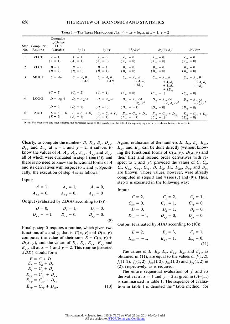
TABLE 1.-THE TABLE METHOD FOR f (X, y) = xV + log x, at x = 1, y = 2
Operation to Define
Step Computer LHS No. Routine Variable adlx adav d2 dx2 d2ldx dY d Id
1 VECT A=1 = Ax = A V = 0 AYX = 0 Ay, = 0 A,, = 0 (A = 1) (Ax = 1) (AY = 0) (Axy = 0) (AX, = 0) (A1Y =0)
2 VECT B = 2 BX = 0 B, = 1 B\x = 0 Bx = 0 B1,, = 0 (B = 2) (Bx = 0) (B, = 1) (BX = 0) (BX = 0) (B,, = 0)
3 MULT C=AB C5 =AxB C, =A,.B C x=A AXB C5B, =As,B C,.=A,.,.B +ABy +AB, +2AX , B, . +A B 2A B1
+AB xt +A Bx + A B, +AB~~~ +A1B5, + ABX
(C= 2) (C 2 =2) (C, = 1) (Cxy = 0) ( =1)(C, ) 4 LOGG D = logA D= A/A Dv = AY/A Dl = A5XXA D2 -AxvA DV =A1,, A
-A2 IA - A5 A2,I (D = 0) (DX = 1) (DV = 0) (DXx = (D5,= 0) (D,5 = 0)
5 ADD E= C+ D E= Cx -4 D = E, = C + DY E= ?Dx X EV = C., + DXV E,, = C5, + D, (E = 2) (EX = 3) (E,5 = - 1) (Ex (, =1) (F, 0)
Note: For each step and each column, the numerical value of the variable on the left of the equality sign is in parentheses below this variable.
Clearly, to compute the numbers D, Dx, Dy, DXX Dxy and DV at x = 1 and y = 2, it suffices to know the values of A, AX? Ay AXX' Axy and AVI all of which were evaluated in step 1 (see (4)), and there is no need to know the functional forms of A and its derivatives with respect to x and y. Specifi- cally, the execution of step 4 is as follows:
Input:
A = 1, Ax= 1, Ay=O0
Axx = 0 Axy 0, AYY =
Output (evaluated by LOGG according to (8)):
D = 0, Dx= 1, Dy= 0,
Dx = - 1, Dxy = O Dyy = 0
(9)
Finally, step 5 requires a routine, which given two functions of x and y; that is, C(x, y) and D(x, y), computes the value of their sum E = C(x, y) + D(x, y), and the values of E., Ey, Exx, Exv and EY, all at x = 1 and y = 2. This routine (denoted ADD) should form
E =C + D EX= Cx + Dx Ey =Cy + Dy
EXX= Cxx + Dxx E =C +D E,y =Cyy+ Dyy(
Again, evaluation of the numbers E, Ex, E`, EXX" Exy and Eyy can be done directly (without know- ing the functional forms of C(x, y), D(x, y) and their first and second order derivatives with re- spect to x and y), provided the values of C, Cx,
Cy cxxQ c, C,y D, DX, D, DXX Dxy and D y are known. Those values, however, were already computed in steps 3 and 4 (see (7) and (9)). Thus, step 5 is executed in the following way:
Input:
C=2, Cx 2, Cy-=1
cxx= ?, cv =1, C,Vy= 0
D =0, DX-1, Dy= O,
Dx= -1, Dxy-O, Dyy =0
Output (evaluated by ADD according to (10)):
E= 2, Ex= 3, Ey 1
E =-, Exy- =1, Ey.1, =0. (11)
The values of E, Ex, Ey EXXF Ex. and EYY, as obtained in (11), are equal to the values of f (1, 2),
fj(I, 2), f(l, 2), fjx(1, 2), fxy(I, 2) and fyy(l 2) in (2), respectively, as is required.
The entire sequential evaluation of f and its derivatives at x = 1 and y = 2 as given in (3)-(11) is summarized in table 1. The sequence of evalua- tion in table 1 is denoted the "table method" for
This content downloaded from 195.34.79.79 on Wed, 25 Jun 2014 05:40:49 AMAll use subject to JSTOR Terms and Conditions
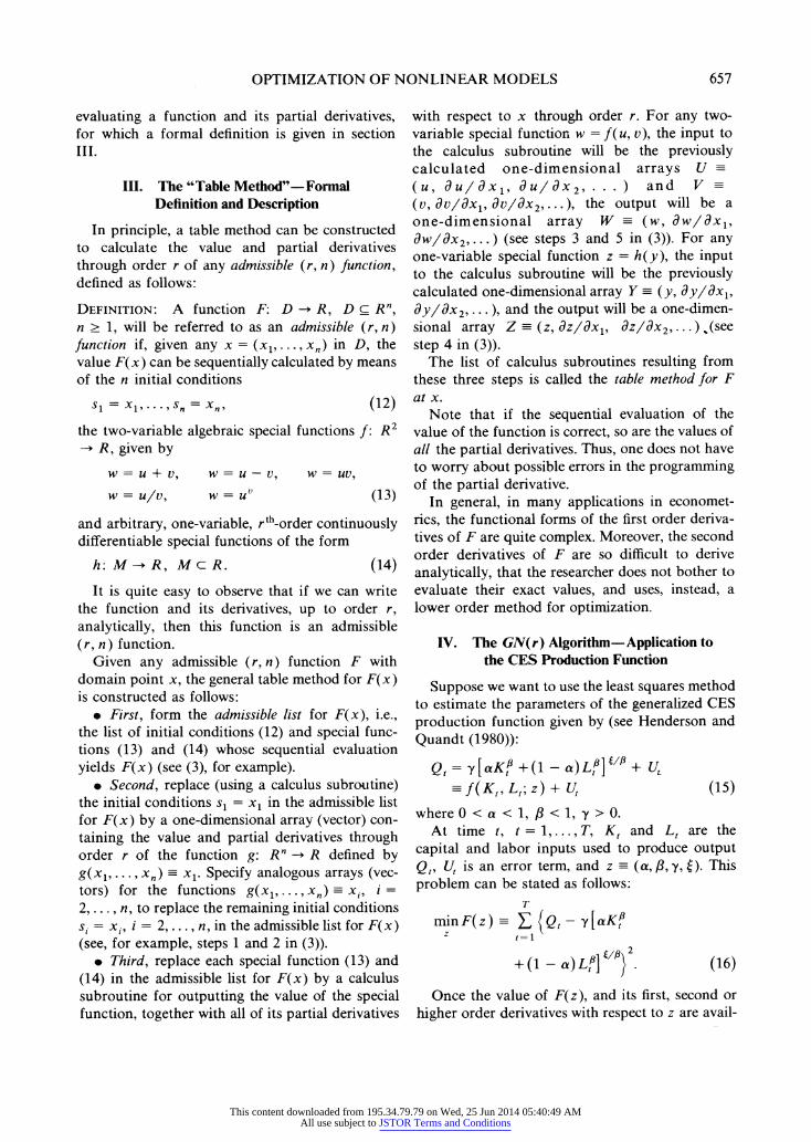
OPTIMIZATION OF NONLINEAR MODELS 657
evaluating a function and its partial derivatives, for which a formal definition is given in section III.
III. The "Table Method"-Formal Definition and Description
In principle, a table method can be constructed to calculate the value and partial derivatives through order r of any admissible (r, n) function, defined as follows:
DEFINITION: A function F: D -- R, D c R , n > 1, will be referred to as an admissible (r, n) function if, given any x = (xl, .. ., xn) in D, the value F(x) can be sequentially calculated by means of the n initial conditions
-l = Xl-...,Sn = xn , (12)
the two-variable algebraic special functions f: R2 R, given by
w = u + v, w = u-v, w = uv,
w=u/v, w=uV (13)
and arbitrary, one-variable, rth_order continuously differentiable special functions of the form
h: M-R, McR. (14)
It is quite easy to observe that if we can write the function and its derivatives, up to order r, analytically, then this function is an admissible (r, n) function.
Given any admissible (r, n) function F with domain point x, the general table method for F(x) is constructed as follows:
* First, form the admissible list for F(x), i.e., the list of initial conditions (12) and special func- tions (13) and (14) whose sequential evaluation yields F(x) (see (3), for example).
* Second, replace (using a calculus subroutine) the initial conditions s, = xl in the admissible list for F(x) by a one-dimensional array (vector) con- taining the value and partial derivatives through order r of the function g: Rn -- R defined by g(xI, ..., xn) xl. Specify analogous arrays (vec- tors) for the functions g(xl, ...,x) x1, i =
2, .. ., n, to replace the remaining initial conditions Si= x, i =2, .. ., n, in the admissible list for F(x) (see, for example, steps 1 and 2 in (3)).
* Third, replace each special function (13) and (14) in the admissible list for F(x) by a calculus subroutine for outputting the value of the special function, together with all of its partial derivatives
with respect to x through order r. For any two- variable special function w = f(u, v), the input to the calculus subroutine will be the previously calculated one-dimensional arrays U (u, du/dxl, du/dx2, . . . ) and V (v, dv/dx1, dv/8x2,...), the output will be a one-dimensional array W (w, dw/dxl, dWIdX2, . . . ) (see steps 3 and 5 in (3)). For any one-variable special function z = h(y), the input to the calculus subroutine will be the previously calculated one-dimensional array Y (y, dy/dxl, dy/dx2,...), and the output will be a one-dimen- sional array Z (z, dz/dxl, dz/dx2, ...) (see step 4 in (3)).
The list of calculus subroutines resulting from these three steps is called the table method for F at x.
Note that if the sequential evaluation of the value of the function is correct, so are the values of all the partial derivatives. Thus, one does not have to worry about possible errors in the programming of the partial derivative.
In general, in many applications in economet- rics, the functional forms of the first order deriva- tives of F are quite complex. Moreover, the second order derivatives of F are so difficult to derive analytically, that the researcher does not bother to evaluate their exact values, and uses, instead, a lower order method for optimization.
IV. The GN(r) Algorithm-Application to the CES Production Function
Suppose we want to use the least squares method to estimate the parameters of the generalized CES production function given by (see Henderson and Quandt (1980)):
t= y[aK + (1 - a)L#]I"/ + Ut
-f(Kt,Lt;z) + Ut (15)
where 0 < a < 1, f < 1, y > 0. At time t, t = 1,. .., T, K, and L, are the
capital and labor inputs used to produce output
Qt, Ut is an error term, and z (a,,8,y, ). This problem can be stated as follows:
T
min F(z)_ Qt{Q,-y [caK, z t=l
+(- a)L,81 } (16)
Once the value of F(z), and its first, second or higher order derivatives with respect to z are avail-
This content downloaded from 195.34.79.79 on Wed, 25 Jun 2014 05:40:49 AMAll use subject to JSTOR Terms and Conditions
658 THE REVIEW OF ECONOMICS AND STATISTICS
able, we can use an iterative algorithm to find the optimal parameters z.
The complete derivation and properties of the general GN(r) algorithm are given in Kalaba and Tishler (1983), and Kalaba, Tishler and Wang (1984). In particular, it is shown that the GN(r) algorithm is a fixed point algorithm with r + 1 (for r = 1, 2, 3) order of convergence, where r + 1 is the highest order derivative to be used. It is easy to show that the Newton-Raphson algorithm is identical to the GN(1) algorithm.
The use of the GN(r) algorithm amounts to solving the system of equations F, = 0 (F, denotes the first order derivative of F with respect to z) using the first, second up to rth order derivatives of F, with respect to z, while neglecting derivatives of order higher than r. In general, when the number of parameters to be estimated is M, one needs to solve iteratively the following equations (i is the iteration index):
zi+1 = zi + S5i (17)
where 3' includes the second up to the M + 1 elements in the first row of the matrix A-1 (if it exists) evaluated at z = z', where
A = [(I); (F1),* , (FM); (F (F1F2), ...
2 M); ... *;( F1r)( F1r- 1F2 M)
(18)
and the expressions in the parentheses are the following column vectors:
( [ dy dy d2y d2y Y dz d1'' dZM' dZ1 dz1dz2
d2y_ d ry dry dy ]
dZ2 dZr' dzr1dZ2 dZzr]
(19)
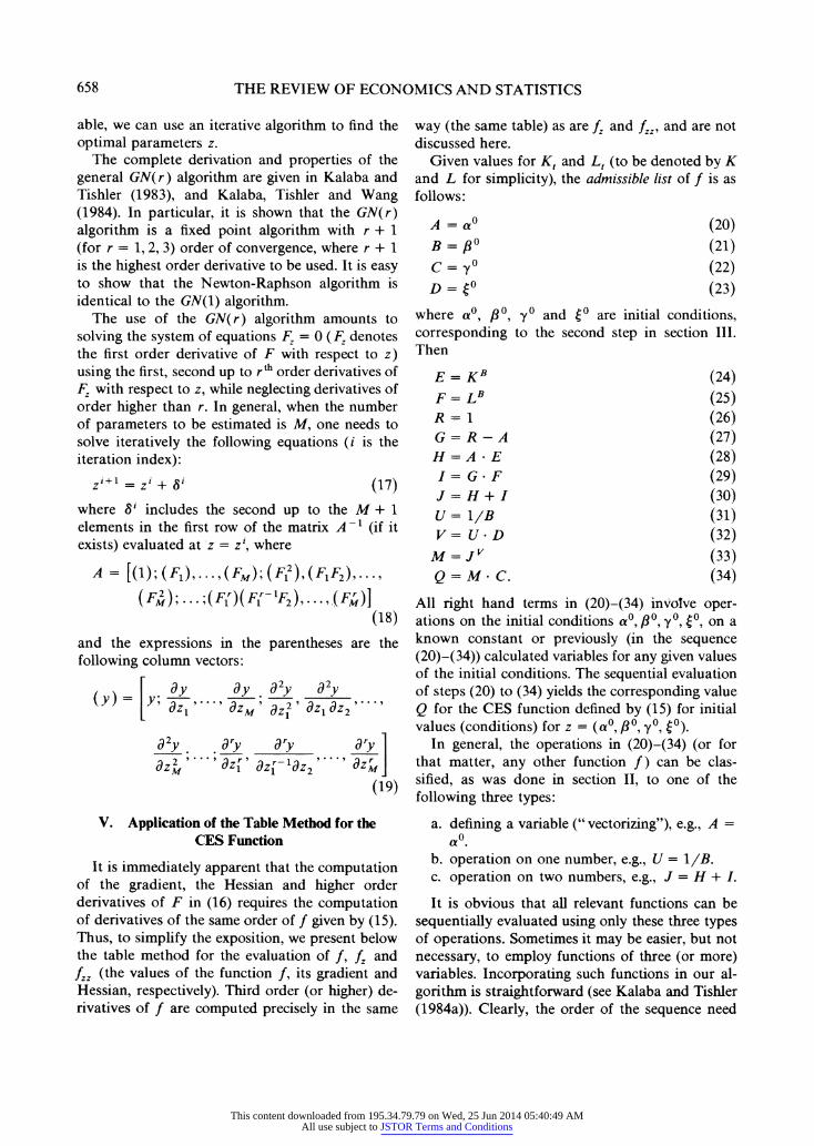
V. Application of the Table Method for the CES Function
It is immediately apparent that the computation of the gradient, the Hessian and higher order derivatives of F in (16) requires the computation of derivatives of the same order of f given by (15). Thus, to simplify the exposition, we present below the table method for the evaluation of f, f, and fzz (the values of the function f, its gradient and Hessian, respectively). Third order (or higher) de- rivatives of f are computed precisely in the same
way (the same table) as are fz and fz' and are not discussed here.
Given values for Kt and Lt (to be denoted by K and L for simplicity), the admissible list of f is as follows:
A = ao (20) ,B = Po(21)
C= y (22) D = V? (23)
where ao, /3,0 yo and (? are initial conditions, corresponding to the second step in section III. Then
E= KB (24) F = LB (25) R= 1 (26) G = R-A (27) H = A * E (28) I= G F (29) J = H+ I (30) U= 1/B (31) V= U- D (32)
M = fv (33) Q = M C. (34)
All right hand terms in (20)-(34) inVolve oper- ations on the initial conditions a0, ,0B y0? , on a known constant or previously (in the sequence (20)-(34)) calculated variables for any given values of the initial conditions. The sequential evaluation of steps (20) to (34) yields the corresponding value Q for the CES function defined by (15) for initial values (conditions) for z = (ao, 380, y?, (0).
In general, the operations in (20)-(34) (or for that matter, any other function f) can be clas- sified, as was done in section II, to one of the following three types:
a. defining a variable (" vectorizing"), e.g., A = 0
b. operation on one number, e.g., U = 1/B. c. operation on two numbers, e.g., J = H + I.
It is obvious that all relevant functions can be sequentially evaluated using only these three types of operations. Sometimes it may be easier, but not necessary, to employ functions of three (or more) variables. Incorporating such functions in our al- gorithm is straightforward (see Kalaba and Tishler (1984a)). Clearly, the order of the sequence need
This content downloaded from 195.34.79.79 on Wed, 25 Jun 2014 05:40:49 AMAll use subject to JSTOR Terms and Conditions
OPTIMIZATION OF NONLINEAR MODELS 659
not be unique. For example, (25) and (26) can be interchanged without affecting the outcome of Q in (34).
The required routines for each type of operation in (20)-(34) are as follows:
(a) A " vectorizing" routine is needed for each variable. In our case the vectorizing routine for a, /B, y and ( in steps (20)-(23) should produce the vectors
(a0, 1, 0, 0, 0, 0, 0 ., 0)
( 0 09 1 0 0 0 0
... , O)
(y?, 0O 0, I O 0, . .0. 0
0)
and
(W9 O, OO, 1,O, ... , O).
The generalization to many variables is ob- vious.
(b) Each operation of one number requires a special routine. That is, in steps (24) and (25) we need a routine which raises a con- stant to a power of a variable. This routine calculates the first and second order deriva- tives of K B (K is constant and B is a function of z) and LB, respectively. In step (26) we need a routine to produce the vector R = (1,0,.. .,0). In step (31) we need a routine to calculate the function and first and second derivatives of a reciprocal of a variable.
(c) Only five two number operations are re- quired for the table method: addition, sub- traction, multiplication, division and raising a variable to the power of another variable. In (20)-(34) we use multiplication in steps (28), (29), (32) and (34). Subtraction is needed in step (27) and addition in step (30). Step (33) requires the use of a routine which raises a variable (J) to the power of another variable (V).
The current software that we use includes all the necessary routines to evaluate the function and its first, up to the fourth order derivatives for any number of variables.
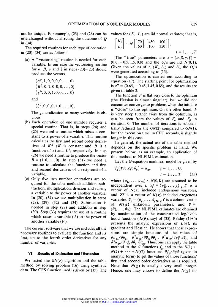
VI. Results of Estimation and Discussion
We tested the GN(r) algorithm and the table method by solving problem (16) using synthetic data. The CES function used is given by (15). The
values for (Kt, Lt) are iid normal variates; that is,
[Kt1r701 450 10011 [ L, JL[L[ 60 ]'L 100 350 ]J]
t = 19,. . .,T. The "true" parameters are z (a, /3, y,) =
(0.6, -0.5, 1.5, 0.8) and the Ut 's are iid N(0, 1). Given the values of z, (Kt, Lt) and Ut, the Qt's were generated according to (15).
The optimization is carried out according to equation (17). The starting point for optimization is zo = (0.65, -0.45, 1.45, 0.85), and the results are given in table 2.
The function F is flat very close to the optimum (the Hessian is almost singular), but we did not encounter convergence problems when the initial z is "close" to this optimum. On the other hand, F is very steep further away from the optimum, as can be seen from the values of FJt and F, in iteration 0. The number of iterations is substan- tially reduced for the GN(2) compared to GN(1), but the execution time, in CPU seconds, is slightly longer in this case.
In general, the actual use of the table method depends on the specific problem at hand. We present below, as an example, an application of this method to NLFIML estimation.
Let the G-equation nonlinear model be given by
fg(Ytg Ztg; Og) = Ugt g = 1,...,G, t = 1, . . ., T (35)
where (ul ,..*, UGt) - N(0, Q) are assumed to be
independent over t. Ytg7 Y=(g)t)' is a vector of N(g) included endogenous variables, and Zg is a vector of K(g) included exogenous variables. 0g = (0gi' ..., 0gM(g))' is a column vector of M( g) unknown parameters, and 0 (O, .. ., Os)'. The NLFIML estimates are obtained by maximization of the concentrated log-likeli- hood function (L(O), say) of (35). Belsley (1980) presents the analytic expressions of L(0), its gradient and Hessian. He shows that these expres- sions are simple functions of the values of dUgt/Idgi, d2Ugt/d0gi d0gj, d2Ugt/dyg dOg and d3ugt/dyg dOgi dOgj. Thus, one can apply the table method to the G functions fg and to the N(1) + N(2) + - - + N(G) functions dfg/dy,gt (given in analytic form) to get the values of those functions' first and second order derivatives as is required. Note that N(g) is usually a very small integer. Hence, one may choose to define the N(g) in-
This content downloaded from 195.34.79.79 on Wed, 25 Jun 2014 05:40:49 AMAll use subject to JSTOR Terms and Conditions
660 THE REVIEW OF ECONOMICS AND STATISTICS
TABLE 2.-RESULTS OF ESTIMATION, T = 25, GN(r) ALGORITHM, r = 1, 2
r Iteration a Estimated Parameters
r No. a ,8y t F F.f F'o F, F,3#
0 0.65 -0.45 1.45 0.85 87.40 349.71 29.20 14.90 -2.03
1 0.6393 -0.5039 1.4496 0.8162 5.51 73.86 5.52 10.12 - 7 0.5590 - 0.0275 1.2286 0.8528 2.58 35.00 3.15 10.48 -
1 15 0.5794 -0.3918 1.6486 0.7788 1.02 -1.49 - 0.14 8.22 - 18 0.5791 -0.3889 1.6461 0.7795 1.01 -0.5 x 10⁻⁹ -0.5 x 10-'1 8.27 -
1 0.6204 - 0.5015 1.4492 0.8106 1.75 27.37 1.87 9.14 4.01 2 0.5511 -0.1174 1.3740 0.8218 1.17 -1.61 - 0.12 9.19 3.44
2 4 0.5769 -0.3670 1.6222 0.7829 1.01 -0.12 -0.01 8.35 4.34 6 0.5791 -0.3889 1.6461 0.7795 1.01 -0.12 x 10⁻⁷ -0.11 x 10⁻⁸ 8.27 4.39
Note: Iteration 0 gives the initial conditions.
cluded endogenous variables in fg(Y g, Z9; 9g) as parameters in addition to 0g, and apply the table method only to the G functions fg. The currently available software of the table method treats all the parameters in a symmetric way. Thus, the savings in programming efforts in this last exten- sion may be offset by the redundant calculations of d2fg/dYg dygi, d3fg/dOgi dOgj d gk and d3fg/dy,g dyft 80gk- It seems possible to further develop the table method to avoid these types of unnecessary computations, but this extension is beyond the scope of this paper.
Extensions and additional examples for the use of the table method and the GN(r) algorithm, as well as suggestions for further research in these areas, are described in Kalaba and Tishler (1983, 1984a, 1984b).
REFERENCES
Belsley, David A., "On the Efficient Computation of the Non- linear Full-Information Maximum-Likelihood Estima- tor," Journal of Econometrics 14 (Oct. 1980), 203-235.
Dennis, J. E., and H. H. W. Mei, "Two New Unconstrained Optimization Algorithms Which Use Function and Gradient Values," Journal of Optimization Theory and Applications 28 (Aug. 1979), 453-482.
Goldfeld, Stephen M., and Richard E. Quandt, Nonlinear
Methods in Econometrics (Amsterdam: North-Holland, 1972).
Henderson, James M., and Richard E. Quandt, Microeconomic Theory, 3rd ed. (New York: McGraw-Hill, 1980).
Hendry, David F., and Frank Srba, "AUTOREG: A Computer Program Library for Dynamic Econometric Models with Autoregressive Errors," in W. T. Dent (ed.), Annals of Applied Econometrics, a supplement to the Journal of Econometrics 12 (Jan. 1980), 85-102.
Kalaba, Robert, Leigh Tesfatsion, and Jone-Lin Wang, "A Finite Algorithm for the Exact Evaluation of Higher- Order Partial Derivatives of Functions of Many Vari- ables," Journal of Mathematical Analysis and Applica- tions 92 (Apr. 1983), 552-563.
Kalaba, Robert, and Asher Tishler, "A Generalized Newton Algorithm Using Higher Order Derivatives," Journal of Optimization Theory and Applications 39 (Jan. 1983), 1-17. , "A Generalized Newton Algorithm to Minimize a Function with Many Variables Using Computer Evaluated Exact Higher Order Derivatives," Journal of Optimization Theory and Applications 42 (Mar. 1984a), 383-395. , "On the Use of the Table Method in Constrained Optimization," Journal of Optimization Theory and Ap- plications 43 (1984b), 157-165.
Kalaba, Robert, Asher Tishler, and Jia Song Wang, "The Rate of Convergence of the GN(r) Algorithm Using the Fixed Point Approach," Journal of Optimization Theory and Applications 43 (Aug. 1984b), 543-555.
Parke, William R., "An Algorithm for FIML and 3SLS Estima- tion of Large Nonlinear Models," Econometrica 50 (Jan. 1982), 81-95.
White, Halbert, "Maximum Likelihood Estimation of Mis- specified Models," Econometrica 50 (Jan. 1980), 1-25.
This content downloaded from 195.34.79.79 on Wed, 25 Jun 2014 05:40:49 AMAll use subject to JSTOR Terms and Conditions


![Derivative-free methods for nonlinear programming with ... · 20 NONLINEAR PROGRAMMING WITH GENERAL LOWER-LEVEL CONSTRAINTS recently published by Conn, Scheinberg and Vicente [9]](https://img.pdfslide.us/doc/110x75/5fb8d6ecfb58283873527d66/derivative-free-methods-for-nonlinear-programming-with-20-nonlinear-programming.jpg)