1

Automatic Construction of Building Footprints fromAirborne LIDAR Data

Keqi Zhang, Jianhua Yan, and Shu-Ching Chen, Senior Member, IEEE,

Abstract— This paper presents a framework that applies aseries of algorithms to automatically extract building footprintsfrom airborne LIDAR measurements. In the proposed frame-work, the ground and non-ground LIDAR measurements arefirst separated using a progressive morphological filter. Then,building measurements are identified from non-ground measure-ments using a region growing algorithm based on the plane-fitting technique. Finally, raw footprints for segmented buildingmeasurements are derived by connecting boundary points, andthe raw footprints are further simplified and adjusted to removenoise caused by irregularly spaced LIDAR measurements. Datasets from urbanized areas including large institutional, commer-cial, and small residential buildings were employed to test theproposed framework. Quantitative analysis showed that the totalof omission and commission errors for extracted footprints forboth institutional and residential areas was about 12%. Theresults demonstrated that the proposed framework identifiedbuilding footprints well.

Index Terms— Airborne LIDAR, building footprint.

I. INTRODUCTION

BUILDING footprints are one of the fundamental GISdata components that can be used to estimate energy

demand, quality of life, urban population, and property taxes[1]. Accurate building footprint data are essential for construc-tion of urban landscape models, assessment of urban heatisland effect, and estimation of building base elevation forflood insurance [2]. In addition, footprint data in combinationwith height values can be used to generate three-dimensional(3D) building models for visualization in GIS. Traditionally,aerial photographs and high-resolution satellite images werethe most effective data sources for extraction of buildingfootprints. Manual derivation of building geometric data froma remote sensing image for a large area is cost prohibitiveand time consuming. Therefore, numerous studies have beendone to develop automated methods to extract footprints [3]-[6]. However, the success of the automated methods is limiteddue to the influence of sun shadow and relief displacement ofhigh buildings in remote sensing images.

Recent emerging airborne light detection and ranging (LI-DAR) technology provides a promising alternative for mea-

Manuscript received June 27, 2005; revised February 23, 2006. This workwas supported by the Florida Hurricane Alliance Research Program sponsoredby National Oceanic and Atmospheric Administration and by the NationalScience Foundation under contract EAR-0518962.

K. Zhang is with the Department of Environmental Studies and Interna-tional Hurricane Research Center, Florida International University, Miami, FL33199 USA (e-mail: zhangk@ fiu.edu).

J. Yan and S.-C. Chen are with the Distributed Multimedia InformationSystem Laboratory, School of Computing and Information Sciences, FloridaInternational University, Miami, FL 33199 USA (e-mail: jyan001@ cs.fiu.edu;chens@cs.fiu.edu;).

suring buildings. Airborne LIDAR systems derive irregularlyspaced 3D point measurements of objects, including ground,buildings, trees, and cars scanned by the laser beneath theaircraft. Compared to aerial photographs and satellite images,LIDAR measurements are not influenced by sun shadow andrelief displacement. However, voluminous point data pose anew challenge for automated extraction of building informa-tion from LIDAR measurements because many raster imageprocessing techniques cannot be directly applied to irregularlyspaced points.

This paper presents algorithms for the extraction of buildingfootprints from LIDAR measurements. The presented workis focused more on 2D footprint extraction than 3D buildingmodels. The paper is arranged as follows. Section II reviewsthe previous work. Section III describes the algorithms thatderive building footprints. Section IV describes the sampleLIDAR data set used by this study and parameters for dataprocessing. Section V examines the results by applying foot-print extraction algorithms to the sample data set and discussesseveral factors influencing footprint extraction algorithms.Section VI includes conclusions.

II. LITERATURE REVIEW

Two steps are involved in extracting a building footprint:identifying building measurements from LIDAR data andderiving the footprint polygon. Two ways are often utilizedto identify building measurements from LIDAR data. One isto separate ground, buildings, trees, and other measurementsfrom LIDAR data simultaneously [7][8]. The more popularway is to separate the ground from non-ground LIDAR mea-surements first and then identify the building points from non-ground measurements [9]-[11]. Numerous algorithms havebeen developed to identify ground measurements from LIDARdata [12]. The non-ground measurements can be derived byremoving identified ground data from a raw data set. Thecritical step is to classify the building and vegetation pointswhich dominate non-ground measurements.

Morgan and Tempfli [9] applied Laplacian and Sobel op-erators to height surfaces to separate building and tree mea-surements. Filin [8] and Morgan and Habib [13] separatedbuilding and tree measurements using the parameters for aplane which fits a LIDAR point and its neighbors within a localwindow. Elberink and Mass [14] segmented LIDAR data usinganisotropic height texture measures. Alharthy and Bethel [15]employed the height difference between the first and last returnmeasurements to distinguish building and tree measurements.The Hough Transform has also been used to identify building

2

points from non-ground measurements [11] or directly fromraw LIDAR data [16][17].

However, these methods suffer from various problems. Forexample, the height differences from first and last returnsdo not work for areas covered by dense trees where laserpulses cannot penetrate. It is difficult to define an optimumvoting size in the parameter space for the Hough Transformbecause local height changes of building roof surfaces arevaried. The region growing algorithm is often employed toidentify building points in a method that uses estimated planeparameters for a point and its neighbors. The processes ofregion growing are variable, depending on the selection of seedpoints. The effect of selecting seed points on segmentationresults has not been examined.

After measurements for a building are identified, a raw foot-print polygon for the building can be derived by connectingall boundary points. However, the raw footprint is often noisybecause of the irregularly spaced LIDAR measurements. It isa challenging task to derive an accurate footprint from a noisyand complex polygon. Alharthy and Bethel [15] employeda histogram of boundary points to generalize the footprintedges by assuming that the buildings have only two dominantdirections that are perpendicular with each other. Based onthe same assumption, Sampath and Shan [18] used the leastsquares model to regularize the footprint edges. However, thisassumption is too strict and cannot be applied to buildingswhose edges are not perpendicular to the dominant directions.It is not uncommon that both commercial and residentialbuildings have some segments that are not parallel to thedominant directions.

The main objective of this paper is to present a frameworkinvolving a series of algorithms for building footprint extrac-tion from LIDAR measurements and an accuracy analysis forthe proposed methods. The framework consists of three majorsteps. First, the non-ground and ground measurements areseparated. Second, building measurements are identified byregion growing using a local plane-fitting technique. Finally,footprints are derived and adjusted based on estimated domi-nant directions.

III. DERIVATION OF BUILDING FOOTPRINTS

A. Separating Ground and Non-Ground Measurements

Morgan and Tempfli [9] showed that classifying ground andnon-ground measurements is a critical step for constructingbuilding footprints. The ground and non-ground measurementsare separated as a first step in the proposed frameworkusing a progressive morphological filter [19]. We selected theprogressive morphological filter because this filter identifiesthe ground and non-ground measurements well for the studyareas which are located in a coastal urban setting with gentleslopes. Alternative filters can also be used in this step if thosefilters can produce a better classification.

Before filtering and building identification, a two-dimensional array was employed to represent points fallingin cells of a mesh overlaying the data set to facilitate thecomputation. The cell size (cs) of the mesh is usually setto be less than the average spacing of LIDAR points to

reduce information loss. Each point measurement from theLIDAR data set is assigned to a cell in terms of its x and ycoordinates. If more than one point falls in the same cell, thepoint with the lowest elevation is selected as the array element.If no point exists in a cell, the array element for the cell isassigned by its nearest neighbor. Since our main concern is toidentify buildings, non-ground measurements whose heightsare less than 2 m were removed to minimize the effect oftrimmed bushes. The heights were derived by subtractingelevations interpolated using identified ground measurementsfrom elevations of non-ground measurements.

B. Identifying Building Measurements

The second step of our method is to identify buildingmeasurements from non-building (mainly vegetation) datausing the region growing algorithm based on a plane-fittingtechnique. Areas of connected non-ground measurements arefound and labeled first by connecting the eight neighbors ofa cell, recursively. For each non-ground measurement area,inside and boundary points are identified. If at least one ofthe eight neighbors of a point is a ground measurement, thepoint is defined as a boundary point. Otherwise, the point isan inside point.

Then, non-ground LIDAR measurements for each areaare segmented by region growing based on a plane-fittingtechnique. Given an inside point p0(x0, y0, z0), a Cartesiancoordinate system (x, y, and z) is established using p0 as theorigin. In this coordinate system, a best fitting plane for p0

and its eight neighbors is derived by using the least squaresmethod. Assume that the plane is defined by:

z = ax+ by + c (1)

The parameters (a, b, c) can be derived by minimizing thesum of squares due to deviations (SSD)

min(SSD) = min∑

(pk)∈M

(zk − hk)2 (2)

where M is a set for p0 and its neighbors, and hk and zk

are observed and plane fitted surface elevations, respectively.Region growing segmentation starts with the selection of

the seed point from the inside points for an area of connectednon-ground measurements. The inside points for the area aresorted based on their SSDs in ascending order. The point withthe minimum SSD is labeled and selected as the first seed pointfor region growing. The neighbors of a seed point are judgedby whether they belong to the same category through a plane-fitting technique. A plane is constructed based on the pointsin the category using a least squares fit. The elevation fromthe candidate point to this plane is compared to a predefinedthreshold ΔhT to select the point. ΔhT is determined by theelevation error of the LIDAR survey and is usually 15-30 cm.If a neighbor is found to be in the same category, it is labeledand added to the category. The neighbors of the growing areaare examined further, and the process is continued until noadditional points can be added into the category. Next, theunlabeled inside points are sorted in terms of their SSDs, andregion growing starts again from a labeled seed point with a

3

minimum SSD. The region-growing processes are repeated foreach non-ground measurement area until all measurements aresegmented.

After non-ground measurements are segmented, patches fornon-building objects are removed by four steps. First, areasof patches are compared with a predefined area thresholdMin Surface (e.g. 5 m2) to eliminate small and fragmentedpatches of vegetation. Second, eliminated small patches in thefirst step representing chimneys, water tanks, and pipe lines ofbuildings are recovered. The condition to include these smallpatches is they are completely surrounded by large patches.Third, isolated boundary points, none of whose eight neighborsis an inside point, are removed. Fourth, the remaining patchesare merged in terms of their connectivity. Through this process,adjacent roof surfaces from the same building, having differentslopes, are merged into a large building patch. Relativelylarge vegetation patches that are not removed in the first stepremain in merged patches, however vegetation patch sizes areusually smaller compared to those of merged building roofs.Therefore, these vegetation patches are removed by comparingtheir area values to a threshold Min Building that approximatesthe minimum area of a building, e.g. 60 m2. The remainingpatches after four operations are classified as building patches.

C. Deriving the Outline of a Building

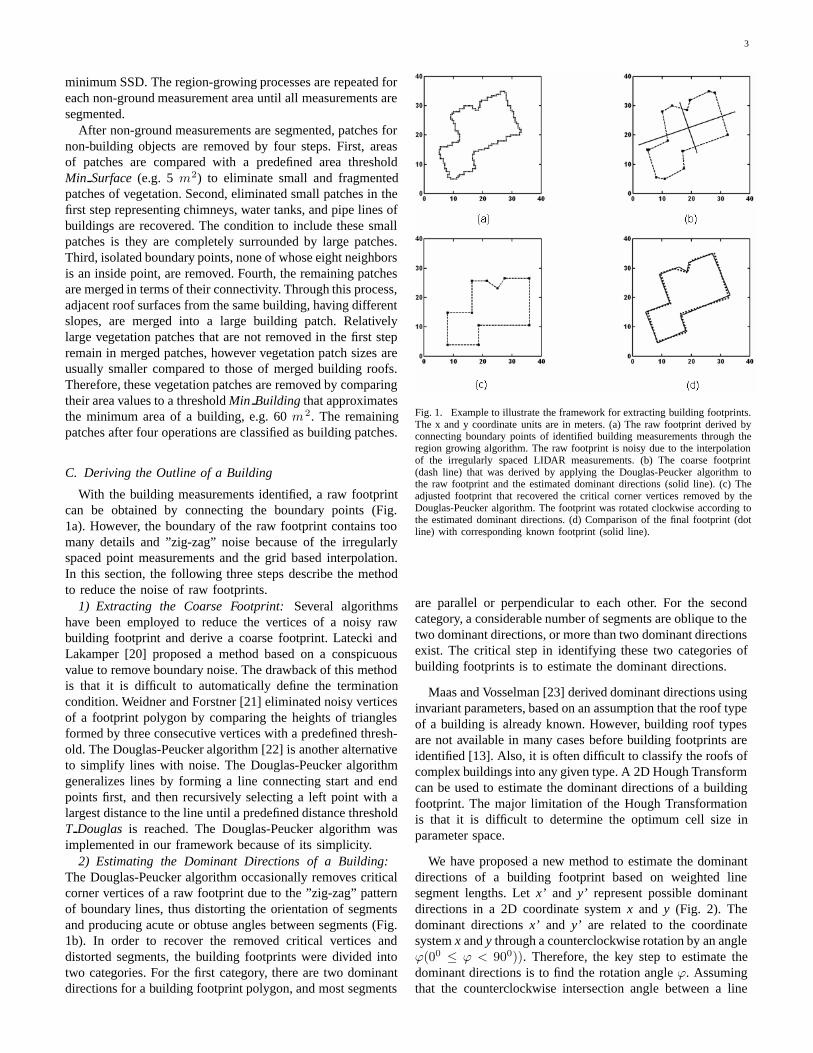
With the building measurements identified, a raw footprintcan be obtained by connecting the boundary points (Fig.1a). However, the boundary of the raw footprint contains toomany details and ”zig-zag” noise because of the irregularlyspaced point measurements and the grid based interpolation.In this section, the following three steps describe the methodto reduce the noise of raw footprints.

1) Extracting the Coarse Footprint: Several algorithmshave been employed to reduce the vertices of a noisy rawbuilding footprint and derive a coarse footprint. Latecki andLakamper [20] proposed a method based on a conspicuousvalue to remove boundary noise. The drawback of this methodis that it is difficult to automatically define the terminationcondition. Weidner and Forstner [21] eliminated noisy verticesof a footprint polygon by comparing the heights of trianglesformed by three consecutive vertices with a predefined thresh-old. The Douglas-Peucker algorithm [22] is another alternativeto simplify lines with noise. The Douglas-Peucker algorithmgeneralizes lines by forming a line connecting start and endpoints first, and then recursively selecting a left point with alargest distance to the line until a predefined distance thresholdT Douglas is reached. The Douglas-Peucker algorithm wasimplemented in our framework because of its simplicity.

2) Estimating the Dominant Directions of a Building:The Douglas-Peucker algorithm occasionally removes criticalcorner vertices of a raw footprint due to the ”zig-zag” patternof boundary lines, thus distorting the orientation of segmentsand producing acute or obtuse angles between segments (Fig.1b). In order to recover the removed critical vertices anddistorted segments, the building footprints were divided intotwo categories. For the first category, there are two dominantdirections for a building footprint polygon, and most segments

Fig. 1. Example to illustrate the framework for extracting building footprints.The x and y coordinate units are in meters. (a) The raw footprint derived byconnecting boundary points of identified building measurements through theregion growing algorithm. The raw footprint is noisy due to the interpolationof the irregularly spaced LIDAR measurements. (b) The coarse footprint(dash line) that was derived by applying the Douglas-Peucker algorithm tothe raw footprint and the estimated dominant directions (solid line). (c) Theadjusted footprint that recovered the critical corner vertices removed by theDouglas-Peucker algorithm. The footprint was rotated clockwise according tothe estimated dominant directions. (d) Comparison of the final footprint (dotline) with corresponding known footprint (solid line).

are parallel or perpendicular to each other. For the secondcategory, a considerable number of segments are oblique to thetwo dominant directions, or more than two dominant directionsexist. The critical step in identifying these two categories ofbuilding footprints is to estimate the dominant directions.

Maas and Vosselman [23] derived dominant directions usinginvariant parameters, based on an assumption that the roof typeof a building is already known. However, building roof typesare not available in many cases before building footprints areidentified [13]. Also, it is often difficult to classify the roofs ofcomplex buildings into any given type. A 2D Hough Transformcan be used to estimate the dominant directions of a buildingfootprint. The major limitation of the Hough Transformationis that it is difficult to determine the optimum cell size inparameter space.

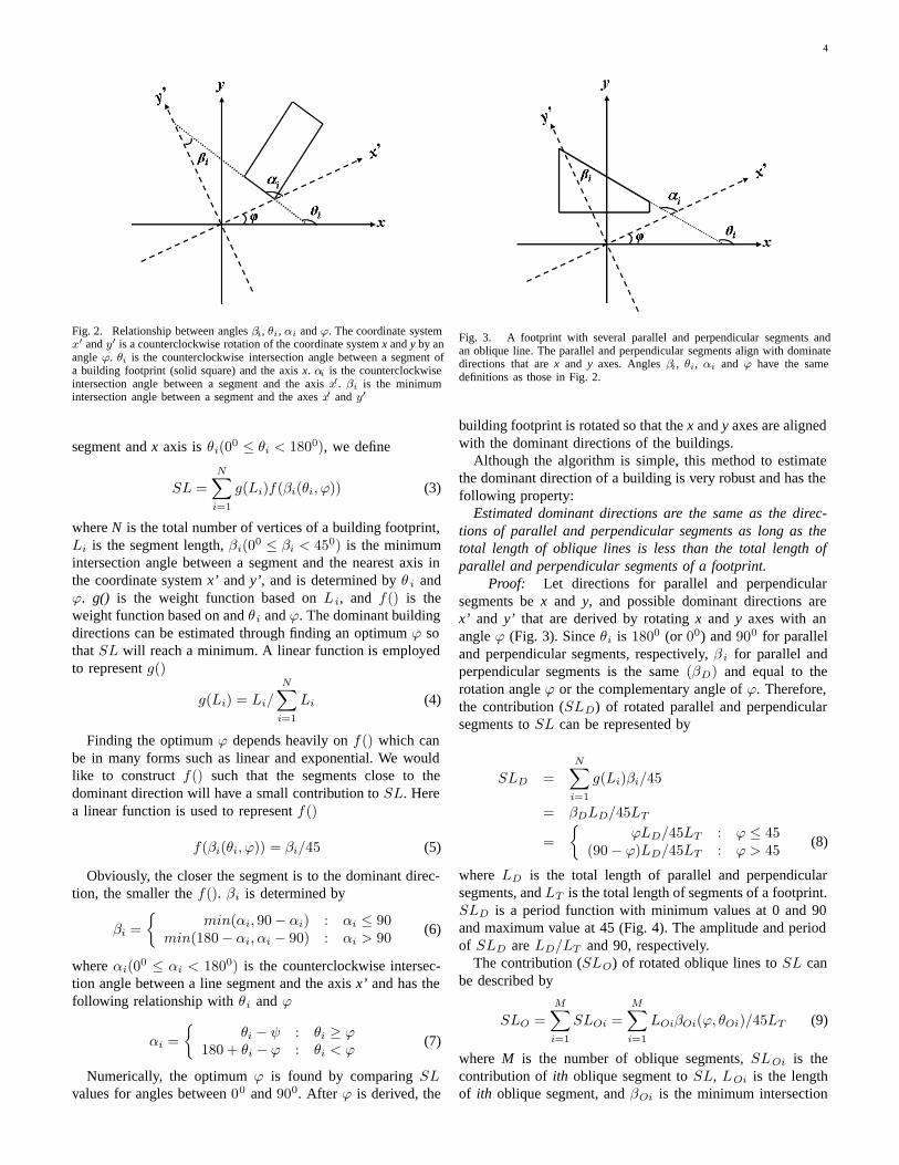
We have proposed a new method to estimate the dominantdirections of a building footprint based on weighted linesegment lengths. Let x’ and y’ represent possible dominantdirections in a 2D coordinate system x and y (Fig. 2). Thedominant directions x’ and y’ are related to the coordinatesystem x and y through a counterclockwise rotation by an angleϕ(00 ≤ ϕ < 900)). Therefore, the key step to estimate thedominant directions is to find the rotation angle ϕ. Assumingthat the counterclockwise intersection angle between a line

4

Fig. 2. Relationship between angles βi, θi, αi and ϕ. The coordinate systemx′ and y′ is a counterclockwise rotation of the coordinate system x and y by anangle ϕ. θi is the counterclockwise intersection angle between a segment ofa building footprint (solid square) and the axis x. αi is the counterclockwiseintersection angle between a segment and the axis x′. βi is the minimumintersection angle between a segment and the axes x′ and y′

segment and x axis is θi(00 ≤ θi < 1800), we define

SL =N∑

i=1

g(Li)f(βi(θi, ϕ)) (3)

where N is the total number of vertices of a building footprint,Li is the segment length, βi(00 ≤ βi < 450) is the minimumintersection angle between a segment and the nearest axis inthe coordinate system x’ and y’, and is determined by θ i andϕ. g() is the weight function based on L i, and f() is theweight function based on and θi and ϕ. The dominant buildingdirections can be estimated through finding an optimum ϕ sothat SL will reach a minimum. A linear function is employedto represent g()

g(Li) = Li/

N∑i=1

Li (4)

Finding the optimum ϕ depends heavily on f() which canbe in many forms such as linear and exponential. We wouldlike to construct f() such that the segments close to thedominant direction will have a small contribution to SL. Herea linear function is used to represent f()

f(βi(θi, ϕ)) = βi/45 (5)

Obviously, the closer the segment is to the dominant direc-tion, the smaller the f(). βi is determined by

βi ={

min(αi, 90 − αi) : αi ≤ 90min(180− αi, αi − 90) : αi > 90 (6)

where αi(00 ≤ αi < 1800) is the counterclockwise intersec-tion angle between a line segment and the axis x’ and has thefollowing relationship with θi and ϕ

αi ={

θi − ψ : θi ≥ ϕ180 + θi − ϕ : θi < ϕ

(7)

Numerically, the optimum ϕ is found by comparing SLvalues for angles between 00 and 900. After ϕ is derived, the

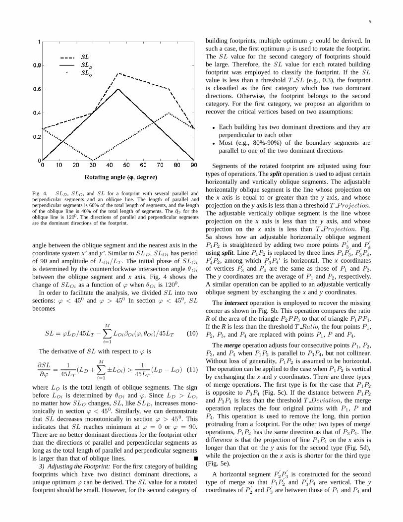
Fig. 3. A footprint with several parallel and perpendicular segments andan oblique line. The parallel and perpendicular segments align with dominatedirections that are x and y axes. Angles βi, θi, αi and ϕ have the samedefinitions as those in Fig. 2.

building footprint is rotated so that the x and y axes are alignedwith the dominant directions of the buildings.

Although the algorithm is simple, this method to estimatethe dominant direction of a building is very robust and has thefollowing property:

Estimated dominant directions are the same as the direc-tions of parallel and perpendicular segments as long as thetotal length of oblique lines is less than the total length ofparallel and perpendicular segments of a footprint.

Proof: Let directions for parallel and perpendicularsegments be x and y, and possible dominant directions arex’ and y’ that are derived by rotating x and y axes with anangle ϕ (Fig. 3). Since θi is 1800 (or 00) and 900 for paralleland perpendicular segments, respectively, β i for parallel andperpendicular segments is the same (βD) and equal to therotation angle ϕ or the complementary angle of ϕ. Therefore,the contribution (SLD) of rotated parallel and perpendicularsegments to SL can be represented by

SLD =N∑

i=1

g(Li)βi/45

= βDLD/45LT

={

ϕLD/45LT : ϕ ≤ 45(90 − ϕ)LD/45LT : ϕ > 45 (8)

where LD is the total length of parallel and perpendicularsegments, and LT is the total length of segments of a footprint.SLD is a period function with minimum values at 0 and 90and maximum value at 45 (Fig. 4). The amplitude and periodof SLD are LD/LT and 90, respectively.

The contribution (SLO) of rotated oblique lines to SL canbe described by

SLO =M∑i=1

SLOi =M∑i=1

LOiβOi(ϕ, θOi)/45LT (9)

where M is the number of oblique segments, SLOi is thecontribution of ith oblique segment to SL, LOi is the lengthof ith oblique segment, and βOi is the minimum intersection

5

Fig. 4. SLD , SLO, and SL for a footprint with several parallel andperpendicular segments and an oblique line. The length of parallel andperpendicular segments is 60% of the total length of segments, and the lengthof the oblique line is 40% of the total length of segments. The θO for theoblique line is 1200. The directions of parallel and perpendicular segmentsare the dominant directions of the footprint.

angle between the oblique segment and the nearest axis in thecoordinate system x’ and y’. Similar to SLD, SLOi has periodof 90 and amplitude of LOi/LT . The initial phase of SLOi

is determined by the counterclockwise intersection angle θOi

between the oblique segment and x axis. Fig. 4 shows thechange of SLOi as a function of ϕ when θOi is 1200.

In order to facilitate the analysis, we divided SL into twosections: ϕ < 450 and ϕ > 450 In section ϕ < 450, SLbecomes

SL = ϕLD/45LT −M∑i=1

LOiβOi(ϕ, θOi)/45LT (10)

The derivative of SL with respect to ϕ is

∂SL

∂ϕ=

145LT

(LD +M∑i=1

±LOi) >1

45LT(LD − LO) (11)

where LO is the total length of oblique segments. The signbefore LOi is determined by θOi and ϕ. Since LD > LO,no matter how SLO changes, SL, like SLD, increases mono-tonically in section ϕ < 450. Similarly, we can demonstratethat SL decreases monotonically in section ϕ > 450. Thisindicates that SL reaches minimum at ϕ = 0 or ϕ = 90.There are no better dominant directions for the footprint otherthan the directions of parallel and perpendicular segments aslong as the total length of parallel and perpendicular segmentsis larger than that of oblique lines.

3) Adjusting the Footprint: For the first category of buildingfootprints which have two distinct dominant directions, aunique optimum ϕ can be derived. The SL value for a rotatedfootprint should be small. However, for the second category of

building footprints, multiple optimum ϕ could be derived. Insuch a case, the first optimum ϕ is used to rotate the footprint.The SL value for the second category of footprints shouldbe large. Therefore, the SL value for each rotated buildingfootprint was employed to classify the footprint. If the SLvalue is less than a threshold T SL (e.g., 0.3), the footprintis classified as the first category which has two dominantdirections. Otherwise, the footprint belongs to the secondcategory. For the first category, we propose an algorithm torecover the critical vertices based on two assumptions:

• Each building has two dominant directions and they areperpendicular to each other

• Most (e.g., 80%-90%) of the boundary segments areparallel to one of the two dominant directions

Segments of the rotated footprint are adjusted using fourtypes of operations. The split operation is used to adjust certainhorizontally and vertically oblique segments. The adjustablehorizontally oblique segment is the line whose projection onthe x axis is equal to or greater than the y axis, and whoseprojection on the y axis is less than a threshold T Projection.The adjustable vertically oblique segment is the line whoseprojection on the x axis is less than the y axis, and whoseprojection on the x axis is less than T Projection. Fig.5a shows how an adjustable horizontally oblique segmentP1P2 is straightened by adding two more points P

′3 and P

′4

using split. Line P1P2 is replaced by three lines P1P′3, P

′3P

′4,

P′4P2, among which P

′3P4

′ is horizontal. The x coordinatesof vertices P

′3 and P

′4 are the same as those of P1 and P2.

The y coordinates are the average of P1 and P2, respectively.A similar operation can be applied to an adjustable verticallyoblique segment by exchanging the x and y coordinates.

The intersect operation is employed to recover the missingcorner as shown in Fig. 5b. This operation compares the ratioR of the area of the triangle P2PP3 to that of triangle P1PP4.If the R is less than the threshold T Ratio, the four points P1,P2, P3, and P4 are replaced with points P1, P and P4.

The merge operation adjusts four consecutive points P1, P2,P3, and P4 when P1P2 is parallel to P3P4, but not collinear.Without loss of generality, P1P2 is assumed to be horizontal.The operation can be applied to the case when P1P2 is verticalby exchanging the x and y coordinates. There are three typesof merge operations. The first type is for the case that P1P2

is opposite to P3P4 (Fig. 5c). If the distance between P1P2

and P3P4 is less than the threshold T Deviation, the mergeoperation replaces the four original points with P1, P andP4. This operation is used to remove the long, thin portionprotruding from a footprint. For the other two types of mergeoperations, P1P2 has the same direction as that of P3P4. Thedifference is that the projection of line P1P4 on the x axis islonger than that on the y axis for the second type (Fig. 5d),while the projection on the x axis is shorter for the third type(Fig. 5e).

A horizontal segment P′2P

′3 is constructed for the second

type of merge so that P1P′2 and P

′3P4 are vertical. The y

coordinates of P′2 and P

′3 are between those of P1 and P4 and

6

Fig. 5. Operations proposed to adjust segments of a footprint (a) split, (b)intersect, (c) first type of merge, (d) second type of merge, and (e) third typeof merge.

are inversely proportional to lengths LP1P2andLP3P4

y = y3 + (y2 − y3)LP1P2

LP1P2 + LP3P4

(12)

where y2 and y3 are coordinates of P2 and P3 on the y axis. Ifthe difference |y2−y3| is less than the threshold T Deviation,the original four consecutive points P1, P2, P3, and P4 areconverted into P1, P

′2, P

′3 and P4 by the merge operation. The

third type of merge operation is illustrated in Fig. 5e. A verticalP

′2P

′3 is constructed by using the average of x coordinates

of P2 and P3 and y coordinate of P2 or P3. If the absolutedifference between y coordinates of P2 and P3 is less thanthreshold T Deviation, the points P1, P2, P3, and P4 arereplaced by P1, P

′2, P

′3 and P4.

The remove operation is designed to remove the redundantvertices of a line. Extra vertices may exist on a segment ofthe footprint after operations split, intersect, and merge areperformed. These extra collinear vertices are eliminated usingthe remove operation immediately after performing one ofthree other operations.

The segments of the first category of building footprints areadjusted iteratively using the four operations starting from asmall value of T Projection. T Projection is incrementedgradually until the percentage of the lengths of horizontal andvertical segments of a footprint is over the predefined threshold

T Footprint. T Footprint is usually set to be between 80%and 90% of the perimeter of the adjusted footprint. Fig. 1cdisplays a building footprint refined from the coarse footprint(Fig. 1b). Corner vertices lost due to the line simplification bythe Douglas-Peucker algorithm were recovered successfully byour footprint adjustment algorithm.

The same operations and procedure are employed to ad-just the second category of building footprints. However,it is not appropriate to use the threshold T Footprint asa termination condition because a considerable number ofsegments are not parallel to the estimated dominant direc-tions. A footprint could be distorted severely if a largeT Footprint is used. Therefore, an alternative terminationcondition for footprint adjustment is employed. The iterationis stopped when T Projection is greater than a thresholdT Projection F inal to avoid adjusting long oblique seg-ments.

IV. DATA PROCESSING

The study area is located at and around the campus ofFlorida International University (FIU), covering 6 km2 oflow relief topography. Surveyed features include residentialhouses, complex buildings, individual trees, forest stands,parking lots, open ground, ponds, roads, and canals. The datawere collected in April 2000 and August 2003 with OptechALTM 1210 and 1233 systems operated by FIU, respectively.The Optech system recorded the coordinates (x, y, z) andintensity of the point measurements corresponding to firstand last laser returns. The 2000 data set consists of threeoverlapping, 400 m wide swaths of 15 cm diameter footprintsspaced approximately 2 m apart. The 2003 data set consistsof five overlapping, 340 m wide swaths of 13 cm diameterfootprints spaced approximately 1 m apart.

Building footprints were extracted from two test LIDARdata sets for the FIU campus and adjacent areas to examinetheir effectiveness. The thresholds used in our experiments forthe FIU campus dataset are listed in Table I. These thresholdswere derived empirically by visually comparing the resultswith gridded raw LIDAR measurements. This is feasiblebecause it took 9, 2, and 0.7 minutes for a PC with 2.8 GHzprocessor and 2 GB RAM to perform morphological filtering,building measurement identification, and footprint derivationfor the FIU campus dataset. A two dimensional array withabout 7.2 million elements was employed to represent raw andinterpolated points covering an area of 1.8 km2. Sensitivityanalysis showed that small changes in these thresholds havelittle impact on the final results.

Aerial photographs, a building footprint map from the FIUPlanning and Facility Management Department, and fieldinvestigation were used to qualitatively and quantitativelyevaluate the derived footprints. The aerial photographs werecollected in 1999 at a resolution of 0.3 m. The Planningand Management Department footprint map was made mainlythrough ground surveying when buildings were constructedand included 62 buildings. All surveyed buildings can be foundon the aerial photographs and they did not change over thetime. Therefore, these buildings can be used to quantify errorsintroduced by our framework.

7

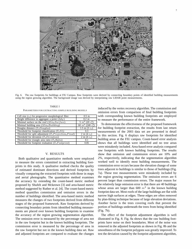
Fig. 6. The raw footprints for buildings at FIU Campus. Raw footprints were derived by connecting boundary points of identified building measurementsusing the region growing algorithm. The background image was derived by interpolating raw LIDAR point measurements.

TABLE I

PARAMETERS FOR EXTRACTING SIMPLE BUILDING MODELS

Cell size (cs) for progressive morphological filter 0.5 mHeight difference to aggregate a point (ΔhT ) 0.2 mMinimal surface on the roof (Min Surface) 5 m2 (20 c2s)Minimal building area (Min Building) 60 m2 (240 c2s)Douglas distance (T Douglas) 1.5 m (3 cs)Threshold for footprint classification (T SL) 0.3Threshold for split adjustment (T Projection F inal) 2 m (4 cs)Threshold for deviation (T Deviation) 2 m (4 cs)Threshold for triangle area ratio (T Ratio) 0.1Threshold for footprint evaluation (T Footprint) 0.85

V. RESULTS

Both qualitative and quantitative methods were employedto measure the errors committed in extracting building foot-prints in this study. A qualitative method checks the qualityof estimated dominant directions and derived footprints byvisually comparing the extracted footprints with those in mapsand aerial photographs. The quantitative method examinesthe accuracy by extending the count-based metric methodproposed by Shufelt and Mckeown [3] and area-based metricmethod suggested by Ruther et al. [4]. The count-based metricmethod quantifies commission and omission errors in thenumber of buildings identified. The area-based metric methodmeasures the changes of two footprints derived from differentstages of the proposed framework. Raw footprints derived byconnecting boundary points from identified building measure-ments are placed over known building footprints to examinethe accuracy of the region growing segmentation algorithm.The omission error is measured by the percentage of area notin the raw footprint but in the known building footprints. Thecommission error is measured by the percentage of area inthe raw footprint but not in the known building data set. Rawand adjusted footprints are compared to evaluate the changes

induced by the vertex recovery algorithm. The commission andomission errors from comparison of final building footprintswith corresponding known building footprints are employedto measure the performance of the entire framework.

To demonstrate the effectiveness of the proposed frameworkfor building footprint extraction, the results from last returnmeasurements of the 2003 data set are presented in detailin this section. Fig. 6 displays raw footprints for identifiedbuilding areas at the FIU campus. Count-based error analysisshows that all buildings were identified and no tree areaswere mistakenly included. Area-based error analysis comparedraw footprints with known building footprints. The resultsshow that omission and commission errors are 10% and2%, respectively, indicating that the segmentation algorithmworked well to identify most building measurements. Thecommission error occurs because the elevation change of sometrees adjacent to buildings is similar to those of buildings (Fig.7a). These tree measurements were mistakenly included bythe region growing segmentation. The omission errors are 6percent larger than commission errors. The major reason forthe relatively large omission error is that there are 40 buildingswhose areas are larger than 600 m2 in the known buildingfootprint data set. Most roofs of the large buildings are flat withnarrow high surfaces at edges. These edges are often removedby plan-fitting technique because of large elevation deviations.Another factor is the trees covering roofs that prevent theportion of buildings underneath the trees from being identified(Fig. 7b).

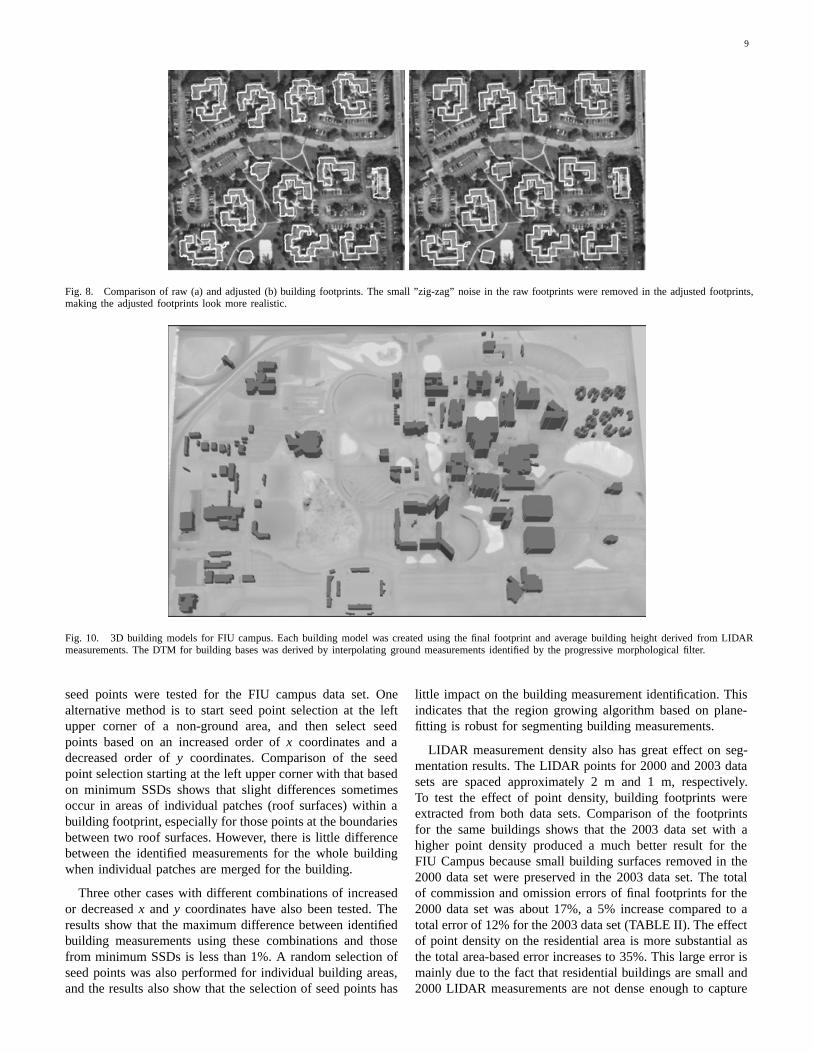
The effect of the footprint adjustment algorithm is wellillustrated in Fig. 8. Fig. 8a shows that the raw building foot-prints have noise on their boundaries. Most of the noise wasremoved in the adjusted footprints as shown in Fig. 8b and thesmoothness of the footprint polygons was greatly improved. Totest the deviation caused by the footprint adjustment algorithm,

8

Fig. 7. Examples of errors caused by the region growing building segmenta-tion algorithm. (a) Commission error (C): the flat tree top next to the buildingis misidentified as a part of the building. (b) Omission error (O): the cornerportions of buildings were missed because the roofs are partially covered bytrees.

raw footprints were compared with adjusted footprints. Theresults show that the deviation is small. About 3% of theraw footprints are not contained in adjusted footprints, and3% of the footprints are mistakenly added to the adjustedfootprints. By visually comparing the adjusted footprints withraw footprints, we found that in most cases the adjustedfootprints preserve the original geometric shape.

The effectiveness of the algorithm to estimate dominantdirections was evaluated by visually examining all final foot-prints. The algorithm worked well for all buildings at theFIU campus. For example, Fig. 9a shows a complex buildingwhich consists of five major parts. The dominant directionswere estimated to be nearly horizontal in terms of three majorrectangles. A circle portion (C in Fig. 9a) was approximatedby several line segments (Fig. 9b). A small oblique rectangle(R in Fig. 9a) whose direction is different from the dominantdirections was also adjusted appropriately.

Fig. 9. The raw (a) and final (b) footprint for a complex building. The xand y coordinate units are meters. Two dominant directions of the footprintare nearly horizontal and vertical. Note that the arc of a circle (C in a) of thefootprint is approximated by a polyline. A small rectangle (R in a) that is notaligned with the dominant directions is well preserved.

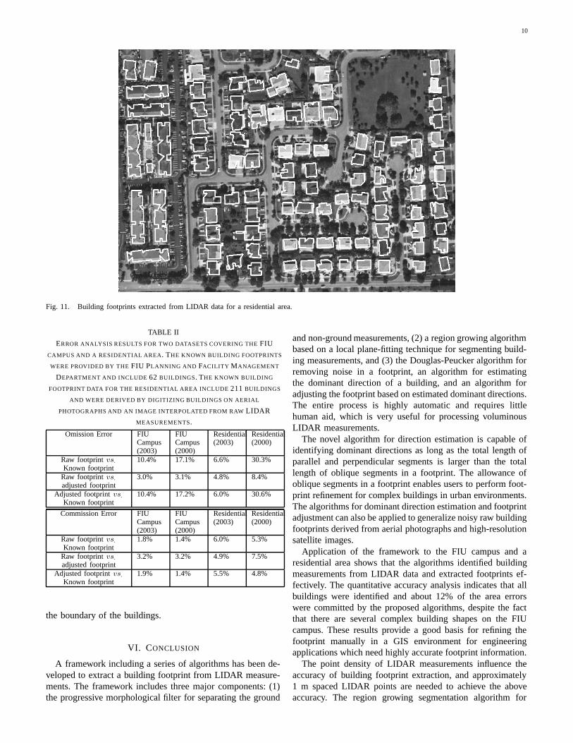
Fig. 10 shows a 3D building map for FIU campus basedon final building footprints and heights. The heights of thebuildings were derived by averaging the elevation differ-ences between building measurements and the digital terrainmodel (DTM) interpolated from ground measurements. Thesebuilding models have been used to construct a 3D syntheticvisual environment to animate hurricane-induced fresh waterflooding at FIU campus. Comparison of 62 final footprintswith footprints from the map provided by the FIU Planningand Facility Management Department shows that 10% of thebuilding footprints were mistakenly removed, and 2% of the

footprints were incorrectly included into the final output byour framework. Both the omission and commission errorsfor the final footprints are almost the same as those causedby the region growing segmentation algorithm. This furtherproves that the deviations caused by the footprint adjustmentalgorithm have little effect on the final result. Therefore, theerrors in final footprints mainly come from the errors beforethe footprint adjustment is performed.

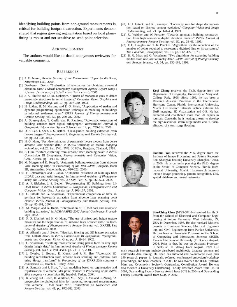
Building extraction results for a residential area are dis-played in Fig. 11. The known building footprint data forthe residential area were derived by digitizing buildings fromaerial photographs. The relief displacement of the residentialhouses in the orthorectified photograph was small due to theirlow heights. The digitized footprints were overlaid over agrid interpolated from raw LIDAR measurements to ensurequality. The data set included 211 building footprints, andthe parameters used by the framework are the same as thoselisted in TABLE I. All buildings were identified from LIDARdata and there were no commission and omission errors fromthe count-based accuracy analysis. Both area-based omissionand commission errors for final footprints were about 6%,indicating that the framework worked well in residential areas.

Several factors influence the accuracy of building measure-ment identification. One of them is the point measurementused in computation. Most airborne LIDAR systems are ca-pable of deriving first and last return measurements for anemitted laser pulse. Both first and last return measurementscan be used to identify the building footprints. However, thereare different advantages and disadvantages in using them. Thefirst return measurements suffer fewer errors from multipathreflections which can be caused by many factors. For example,when a laser pulse hits glass walls or windows, it can enterthe room and bounce several times before it finally reachesthe sensor. The multipath reflection of a laser pulse can leadto incorrect low elevation measurements for the roof of abuilding. These low elevation points are often removed asground measurements by the progressive morphological filter,resulting in small holes in the building footprint. There aremany more multipath errors in the last return measurementsthan in the first return measurements in our data set. However,the last return measurements have more of a chance topenetrate into the vegetation and reach the ground. This helpsthe filter to separate the ground and non-ground measurements.Also, the last return measurements display more spatial changethan the first return in tree areas, which helps separate thebuilding measurements from tree measurements. The currentbuilding identification methods have been applied to both firstand last return data in the study area. It was found that thelast return measurements have a better overall performance.Improvement of the current algorithms by combining the firstand last return measurements need to be further investigated.

The performance of the region growing algorithm to seg-ment building measurements in the proposed framework iscritical to the footprint extraction. The processes of regiongrowing segmentation rely on the selection of seed points.In our algorithm, the seed points are selected in terms ofminimum SSDs based on a plane-fitting technique. To examinethe robustness of the algorithm, other methods for selecting

9

Fig. 8. Comparison of raw (a) and adjusted (b) building footprints. The small ”zig-zag” noise in the raw footprints were removed in the adjusted footprints,making the adjusted footprints look more realistic.

Fig. 10. 3D building models for FIU campus. Each building model was created using the final footprint and average building height derived from LIDARmeasurements. The DTM for building bases was derived by interpolating ground measurements identified by the progressive morphological filter.

seed points were tested for the FIU campus data set. Onealternative method is to start seed point selection at the leftupper corner of a non-ground area, and then select seedpoints based on an increased order of x coordinates and adecreased order of y coordinates. Comparison of the seedpoint selection starting at the left upper corner with that basedon minimum SSDs shows that slight differences sometimesoccur in areas of individual patches (roof surfaces) within abuilding footprint, especially for those points at the boundariesbetween two roof surfaces. However, there is little differencebetween the identified measurements for the whole buildingwhen individual patches are merged for the building.

Three other cases with different combinations of increasedor decreased x and y coordinates have also been tested. Theresults show that the maximum difference between identifiedbuilding measurements using these combinations and thosefrom minimum SSDs is less than 1%. A random selection ofseed points was also performed for individual building areas,and the results also show that the selection of seed points has

little impact on the building measurement identification. Thisindicates that the region growing algorithm based on plane-fitting is robust for segmenting building measurements.

LIDAR measurement density also has great effect on seg-mentation results. The LIDAR points for 2000 and 2003 datasets are spaced approximately 2 m and 1 m, respectively.To test the effect of point density, building footprints wereextracted from both data sets. Comparison of the footprintsfor the same buildings shows that the 2003 data set with ahigher point density produced a much better result for theFIU Campus because small building surfaces removed in the2000 data set were preserved in the 2003 data set. The totalof commission and omission errors of final footprints for the2000 data set was about 17%, a 5% increase compared to atotal error of 12% for the 2003 data set (TABLE II). The effectof point density on the residential area is more substantial asthe total area-based error increases to 35%. This large error ismainly due to the fact that residential buildings are small and2000 LIDAR measurements are not dense enough to capture

10

Fig. 11. Building footprints extracted from LIDAR data for a residential area.

TABLE II

ERROR ANALYSIS RESULTS FOR TWO DATASETS COVERING THE FIU

CAMPUS AND A RESIDENTIAL AREA. THE KNOWN BUILDING FOOTPRINTS

WERE PROVIDED BY THE FIU PLANNING AND FACILITY MANAGEMENT

DEPARTMENT AND INCLUDE 62 BUILDINGS. THE KNOWN BUILDING

FOOTPRINT DATA FOR THE RESIDENTIAL AREA INCLUDE 211 BUILDINGS

AND WERE DERIVED BY DIGITIZING BUILDINGS ON AERIAL

PHOTOGRAPHS AND AN IMAGE INTERPOLATED FROM RAW LIDAR

MEASUREMENTS.

Omission Error FIUCampus(2003)

FIUCampus(2000)

Residential(2003)

Residential(2000)

Raw footprint vs.

Known footprint10.4% 17.1% 6.6% 30.3%

Raw footprint vs.

adjusted footprint3.0% 3.1% 4.8% 8.4%

Adjusted footprint vs.

Known footprint10.4% 17.2% 6.0% 30.6%

Commission Error FIUCampus(2003)

FIUCampus(2000)

Residential(2003)

Residential(2000)

Raw footprint vs.

Known footprint1.8% 1.4% 6.0% 5.3%

Raw footprint vs.

adjusted footprint3.2% 3.2% 4.9% 7.5%

Adjusted footprint vs.

Known footprint1.9% 1.4% 5.5% 4.8%

the boundary of the buildings.

VI. CONCLUSION

A framework including a series of algorithms has been de-veloped to extract a building footprint from LIDAR measure-ments. The framework includes three major components: (1)the progressive morphological filter for separating the ground

and non-ground measurements, (2) a region growing algorithmbased on a local plane-fitting technique for segmenting build-ing measurements, and (3) the Douglas-Peucker algorithm forremoving noise in a footprint, an algorithm for estimatingthe dominant direction of a building, and an algorithm foradjusting the footprint based on estimated dominant directions.The entire process is highly automatic and requires littlehuman aid, which is very useful for processing voluminousLIDAR measurements.

The novel algorithm for direction estimation is capable ofidentifying dominant directions as long as the total length ofparallel and perpendicular segments is larger than the totallength of oblique segments in a footprint. The allowance ofoblique segments in a footprint enables users to perform foot-print refinement for complex buildings in urban environments.The algorithms for dominant direction estimation and footprintadjustment can also be applied to generalize noisy raw buildingfootprints derived from aerial photographs and high-resolutionsatellite images.

Application of the framework to the FIU campus and aresidential area shows that the algorithms identified buildingmeasurements from LIDAR data and extracted footprints ef-fectively. The quantitative accuracy analysis indicates that allbuildings were identified and about 12% of the area errorswere committed by the proposed algorithms, despite the factthat there are several complex building shapes on the FIUcampus. These results provide a good basis for refining thefootprint manually in a GIS environment for engineeringapplications which need highly accurate footprint information.

The point density of LIDAR measurements influence theaccuracy of building footprint extraction, and approximately1 m spaced LIDAR points are needed to achieve the aboveaccuracy. The region growing segmentation algorithm for

11

identifying building points from non-ground measurements iscritical for building footprint extraction. Experiments demon-strated that region growing segmentation based on local plane-fitting is robust and not sensitive to seed point selection.

ACKNOWLEGMENT

The authors would like to thank anonymous reviewers forvaluable comments.

REFERENCES

[1] J. R. Jensen, Remote Sensing of the Environment. Upper Saddle River,NJ:Prentice Hall, 2000.

[2] Dewberry Davis, ”Evaluation of alternatives in obtaining structuralelevation data,” Federal Emergency Management Agency Report (http ://www.fema.gov/nfip/alt elevations.shtm), 2005

[3] J. A. Shufelt and D. M. Mckeown, ”Fusion of monocular cues to detectman-made structures in aerial imagery,” Computer Vision Graphics andImage Understanding, vol. 57, pp. 307-330, 1993.

[4] H. Ruther, H. M. Martine, and E. G. Mtalo, ”Application of snakes anddynamic programming optimization technique in modeling of buildingsin informal settlement areas,” ISPRS Journal of Photogrammetry andRemote Sensing, vol. 56, pp. 269-282, 2002.

[5] A. Strassopolou, T. Caelli, and R. Ramirez, ”Automatic extraction ofbuilding statistics from digital orthographs,” International Journal ofGeographic Information System Science, vol. 14, pp. 759-814, 2000.

[6] D. S. Lee, J. Shan, J. S. Bethel, ”Class-guided building extraction fromIkonos imagery,” Photogrammetric Engineering and Remote Sensing, vol.69, pp.143-150, 2003.

[7] H. G. Maas, ”Fast determination of parametric house models from denseairborne laser scanner data,” in ISPRS workshop on mobile mappingtechnology, vol.32, Part 2W1, 5W1, IC5/3W, Bangkok, Thailand, 1999.

[8] S. Filin, ”Surface clustering from airborne laser scanning data,” in ISPRSCommission III Symposium, Photogrammetric and Computer Vision,Graz, Austria, pp. 119-124, 2002.

[9] M. Morgan and K. Tempfli, ”Automatic building extraction from airbornelaser scanning data,” in Proceeding of the 19th ISPRS Congress, Book3B, Amsterdam, Netherlands, pp. 616-623, 2000.

[10] F. Rottensteiner and J. Jansa, ”Automatic extraction of buildings fromLIDAR data and aerial images,” in International Archives of Photogram-metry and Remote Sensing, vol. XXXIV, Part IX, pp. 569-574, 2002.

[11] A. F. Elaksher, J. S. Bethel, ”Reconstructing 3D Buildings from LI-DAR Data,” in ISPRS Commission III Symposium, Photogrammetric andComputer Vision, Graz, Austria, pp. A 102-107, 2002.

[12] G. Sithole and G. Vosselman, ”Experimental comparison of filter al-gorithms for bare-earth extraction from airborne laser scanning pointclouds.” ISPRS Journal of Photogrammetry and Remote Sensing, Vol.59, pp. 85-101, 2004.

[13] M. Morgan and A. Habib, ”Interpolation of LIDAR data and automaticbuilding extraction,” in ACSM-ASPRS 2002 Annual Conference Proceed-ings, 2002.

[14] S. O. Elberink and H. G. Maas, ”The use of anisotropic height texturemeasures for the segmentation of airborne laser scanner data,” in Inter-national Archive of Photogrammetry Remote Sensing, vol. XXXIII, PartB3/2, pp. 678-684, 2000.

[15] A. Alharthy and J. Bethel, ”Heuristic filtering and 3D feature extractionfrom LIDAR data”, in ISPRS Commission III Symposium, Photogram-metric and Computer Vision, Graz, pp. A 29-34, 2002.

[16] G. Vosselman, ”Building reconstruction using planar faces in very highdensity height data,” in International Archive of Photogrammetry RemoteSensing, vol. XXXIV, Part 3/W4, pp. 211-218, 2001.

[17] J. Overby, L. Bodum, E. Kjems, and P. M. Ilse, ”Automatic 3Dbuilding reconstruction from airborne laser scanning and cadastral datausing Hough transform,” in Proceeding of the ISPRS 20th congress -commission III, Istanbul, Turkey, 2004.

[18] A. Sampath and J. Shan, ”Urban modeling based on segmentation andregularization of airborne lidar point clouds,” in Proceeding of the ISPRS20th congress - commission III, Istanbul, Turkey, 2004.

[19] K. Zhang, S-C. Chen, D. Whitman, M-L. Shyu, J. Yan and C. Zhang, ”Aprogressive morphological filter for removing non-ground measurementsfrom airborne LIDAR data,” IEEE Transactions on Geoscience andRemote Sensing, vol. 41, pp. 872-882, 2003.

[20] L. J. Latecki and R. Lakamper, ”Convexity rule for shape decomposi-tion based on discrete contour evolution,” Computer Vision and ImageUnderstanding, vol. 73, pp. 441-454, 1999.

[21] U. Weidner and W. Forstner, ”Towards automatic building reconstruc-tion from high resolution digital elevation models,” ISPRS Journal ofPhotogrammetry Remote Sensing, vol. 50, pp. 38-49, 1995.

[22] D.H. Douglas and T. K. Peucker, ”Algorithms for the reduction of thenumber of points required to represent a digitized line or its caricature,”The Canadian Cartographer, vol. 10, pp. 112 -122, 1973.

[23] H. G. Maas and G. Vosselman, ”Two algorithms for extracting buildingmodels from raw laser altimetry data,” ISPRS Journal of Photogrammetryand Remote Sensing, vol. 54, pp. 153-163, 1999.

Keqi Zhang received the Ph.D. degree from theDepartment of Geography, University of Maryland,College Park, 1998. Since 1999, he has been aResearch Assistant Professor in the InternationalHurricane Center, Florida International University,Miami. His research interests include airborne LI-DAR mapping, 3D Visualization and GIS. He hasauthored and coauthored more than 20 papers injournals. Currently, he is leading a team to developthe high-resolution storm surge model and 3D visu-alization of storm surge flooding.

Jianhua Yan received the M.S. degree from theInstitute of Image Processing and Pattern Recogni-tion, Shanghai Jiaotong University, Shanghai, China,in 2000. He is currently pursuing the Ph.D. degreeat the School of Computer Science, Florida Inter-national University, Miami. His research interestsinclude image processing, pattern recognition, GIS,spatial database and neural networks.

Shu-Ching Chen (M’95-SM’04) received his Ph.D.from the School of Electrical and Computer Engi-neering at Purdue University, West Lafayette, IN,USA in December, 1998. He also received Master.sdegrees in Computer Science, Electrical Engineer-ing, and Civil Engineering from Purdue University.He has been an Associate Professor in the Schoolof Computing and Information Sciences (SCIS),Florida International University (FIU) since August,2004. Prior to that, he was an Assistant Professorin SCIS at FIU dating from August, 1999. His

main research interests include distributed multimedia database systems andmultimedia data mining. Dr. Chen has authored and co-authored more than140 research papers in journals, refereed conference/symposium/workshopproceedings, and book chapters. In 2005, he was awarded the IEEE Systems,Man, and Cybernetics Society’s Outstanding Contribution Award. He wasalso awarded a University Outstanding Faculty Research Award from FIU in2004, Outstanding Faculty Service Award from SCIS in 2004 and OutstandingFaculty Research Award from SCIS in 2002.