Embed Size (px)
Citation preview
AUTOMATIC CLASSIFICATION OF DIGITAL
COMMUNICATION SIGNAL MODULATIONS
A thesis submitted for the degree of Doctor of Philosophy
by
ZHECHEN ZHU
Department of Electronic and Computer Engineering Brunel
University London October 2014
Abstract
Automatic modulation classification detects the modulation type of received communication
signals. It has important applications in military scenarios to facilitate jamming, intelligence,
surveillance, and threat analysis. The renewed interest from civilian scenes has been fuelled
by the development of intelligent communications systems such as cognitive radio and soft-
ware defined radio. More specifically, it is complementary to adaptive modulation and coding
where a modulation can be deployed from a set of candidates according to the channel con-
dition and system specification for improved spectrum efficiency and link reliability. In this
research, we started by improving some existing methods for higher classification accuracy
but lower complexity. Machine learning techniques such as k-nearest neighbour and sup-
port vector machine have been adopted for simplified decision making using known features.
Logistic regression, genetic algorithm and genetic programming have been incorporated for
improved classification performance through feature selection and combination. We have also
developed a new distribution test based classifier which is tailored for modulation classifica-
tion with the inspiration from Kolmogorov-Smirnov test. The proposed classifier is shown to
have improved accuracy and robustness over the standard distribution test. For blind classi-
fication in imperfect channels, we developed the combination of minimum distance centroid
estimator and non-parametric likelihood function for blind modulation classification without
the prior knowledge on channel noise. The centroid estimator provides joint estimation of
channel gain and carrier phase offset where both can be compensated in the following non-
parametric likelihood function. The non-parametric likelihood function, in the meantime,
provide likelihood evaluation without a specifically assumed noise model. The combination
has shown to have higher robustness when different noise types are considered. To push mod-
ulation classification techniques into a more timely setting, we also developed the principle
for blind classification in MIMO systems. The classification is achieved through expecta-
tion maximization channel estimation and likelihood based classification. Early results have
shown bright prospect for the method while more work is needed to further optimize the
method and to provide a more thorough validation.
i
Contents
1 Introduction 1
1.1 Motivation . . . . . . . . . . . . . . . . . . . . . . . . . . . . . . . . . . . . . 1
1.1.1 Military applications . . . . . . . . . . . . . . . . . . . . . . . . . . . . 1
1.1.2 Civilian applications . . . . . . . . . . . . . . . . . . . . . . . . . . . . 3
1.2 Problem statement . . . . . . . . . . . . . . . . . . . . . . . . . . . . . . . . . 5
1.3 Summary of contributions . . . . . . . . . . . . . . . . . . . . . . . . . . . . . 6
1.4 Thesis organization . . . . . . . . . . . . . . . . . . . . . . . . . . . . . . . . . 7
1.5 List of publications . . . . . . . . . . . . . . . . . . . . . . . . . . . . . . . . . 9
2 Signal Model and Existing Methods 11
2.1 Introduction . . . . . . . . . . . . . . . . . . . . . . . . . . . . . . . . . . . . . 11
2.2 Signal model in AWGN channels . . . . . . . . . . . . . . . . . . . . . . . . . 12
2.3 Signal model in fading channels . . . . . . . . . . . . . . . . . . . . . . . . . . 13
2.4 Signal model in non-Gaussian channels . . . . . . . . . . . . . . . . . . . . . . 15
2.5 Likelihood based classifiers . . . . . . . . . . . . . . . . . . . . . . . . . . . . 17
2.5.1 Maximum likelihood classifier . . . . . . . . . . . . . . . . . . . . . . . 17
2.5.2 Likelihood ratio test classifier . . . . . . . . . . . . . . . . . . . . . . . 19
2.6 Distribution test based classifiers . . . . . . . . . . . . . . . . . . . . . . . . . 22
2.6.1 One-sample KS test . . . . . . . . . . . . . . . . . . . . . . . . . . . . 22
2.6.2 Two-sample KS test . . . . . . . . . . . . . . . . . . . . . . . . . . . . 25
2.7 Feature based classifiers . . . . . . . . . . . . . . . . . . . . . . . . . . . . . . 26
ii
2.7.1 Signal spectral based features . . . . . . . . . . . . . . . . . . . . . . . 26
2.7.2 High-order statistics based features . . . . . . . . . . . . . . . . . . . . 29
2.8 Summary . . . . . . . . . . . . . . . . . . . . . . . . . . . . . . . . . . . . . . 33
3 Machine Learning for Modulation Classification 34
3.1 Introduction . . . . . . . . . . . . . . . . . . . . . . . . . . . . . . . . . . . . . 34
3.2 Machine learning based classifiers . . . . . . . . . . . . . . . . . . . . . . . . . 35
3.2.1 K-nearest neighbour classifier . . . . . . . . . . . . . . . . . . . . . . . 35
3.2.2 Support vector machine classifier . . . . . . . . . . . . . . . . . . . . . 38
3.3 Feature selection and combination . . . . . . . . . . . . . . . . . . . . . . . . 41
3.3.1 Logistic regression . . . . . . . . . . . . . . . . . . . . . . . . . . . . . 41
3.3.2 Genetic algorithm . . . . . . . . . . . . . . . . . . . . . . . . . . . . . 42
3.3.3 Genetic programming . . . . . . . . . . . . . . . . . . . . . . . . . . . 44
3.4 Summary . . . . . . . . . . . . . . . . . . . . . . . . . . . . . . . . . . . . . . 58
4 Distribution Test Based Classifiers 59
4.1 Introduction . . . . . . . . . . . . . . . . . . . . . . . . . . . . . . . . . . . . . 59
4.2 Optimized distribution sampling test . . . . . . . . . . . . . . . . . . . . . . . 60
4.2.1 Phase offset compensation . . . . . . . . . . . . . . . . . . . . . . . . . 60
4.2.2 Sampling location optimization . . . . . . . . . . . . . . . . . . . . . . 62
4.2.3 Test statistics and decision making . . . . . . . . . . . . . . . . . . . . 65
4.2.4 Simulations and numerical results . . . . . . . . . . . . . . . . . . . . 67
4.3 Distribution based features . . . . . . . . . . . . . . . . . . . . . . . . . . . . 80
4.3.1 Optimization of sampling locations . . . . . . . . . . . . . . . . . . . . 82
4.3.2 Feature extraction . . . . . . . . . . . . . . . . . . . . . . . . . . . . . 84
4.3.3 Feature combination . . . . . . . . . . . . . . . . . . . . . . . . . . . . 84
4.3.4 Classification decision making . . . . . . . . . . . . . . . . . . . . . . . 86
4.3.5 Simulations and numerical results . . . . . . . . . . . . . . . . . . . . 89
4.4 Summary . . . . . . . . . . . . . . . . . . . . . . . . . . . . . . . . . . . . . . 92
iii

5 Modulation Classification with Unknown Noise 94
5.1 Introduction . . . . . . . . . . . . . . . . . . . . . . . . . . . . . . . . . . . . . 94
5.2 Classification strategy . . . . . . . . . . . . . . . . . . . . . . . . . . . . . . . 97
5.3 Centroid estimation . . . . . . . . . . . . . . . . . . . . . . . . . . . . . . . . 98
5.3.1 Constellation segmentation estimator . . . . . . . . . . . . . . . . . . . 98
5.3.2 Minimum distance estimator . . . . . . . . . . . . . . . . . . . . . . . 104
5.4 Non-parametric likelihood function . . . . . . . . . . . . . . . . . . . . . . . . 107
5.5 Simulations and numerical results . . . . . . . . . . . . . . . . . . . . . . . . . 111
5.5.1 AWGN channel . . . . . . . . . . . . . . . . . . . . . . . . . . . . . . . 113
5.5.2 Fading channel . . . . . . . . . . . . . . . . . . . . . . . . . . . . . . . 117
5.5.3 Non-Gaussian channel . . . . . . . . . . . . . . . . . . . . . . . . . . . 121
5.5.4 Complexity . . . . . . . . . . . . . . . . . . . . . . . . . . . . . . . . . 122
5.6 Summary . . . . . . . . . . . . . . . . . . . . . . . . . . . . . . . . . . . . . . 122
6 Blind Modulation Classification for MIMO systems 124
6.1 Introduction . . . . . . . . . . . . . . . . . . . . . . . . . . . . . . . . . . . . . 124
6.2 Signal model in MIMO systems . . . . . . . . . . . . . . . . . . . . . . . . . . 125
6.3 EM channel estimation . . . . . . . . . . . . . . . . . . . . . . . . . . . . . . . 126
6.3.1 Evaluation step . . . . . . . . . . . . . . . . . . . . . . . . . . . . . . . 127
6.3.2 Maximization step . . . . . . . . . . . . . . . . . . . . . . . . . . . . . 128
6.3.3 Termination . . . . . . . . . . . . . . . . . . . . . . . . . . . . . . . . . 129
6.4 Maximum likelihood classifier . . . . . . . . . . . . . . . . . . . . . . . . . . . 129
6.5 Simulation and numerical results . . . . . . . . . . . . . . . . . . . . . . . . . 130
6.6 Summary . . . . . . . . . . . . . . . . . . . . . . . . . . . . . . . . . . . . . . 136
7 Conclusions 137
Appendix A: Minimum Distance Centroid Estimation 149
Appendix B: Iterative Minimum Distance Estimator 152
iv

Appendix C: Non-parametric Likelihood Function 154
v
List of Figures
1.1 Application of AMC in military electronic warfare systems. . . . . . . . . . . 2
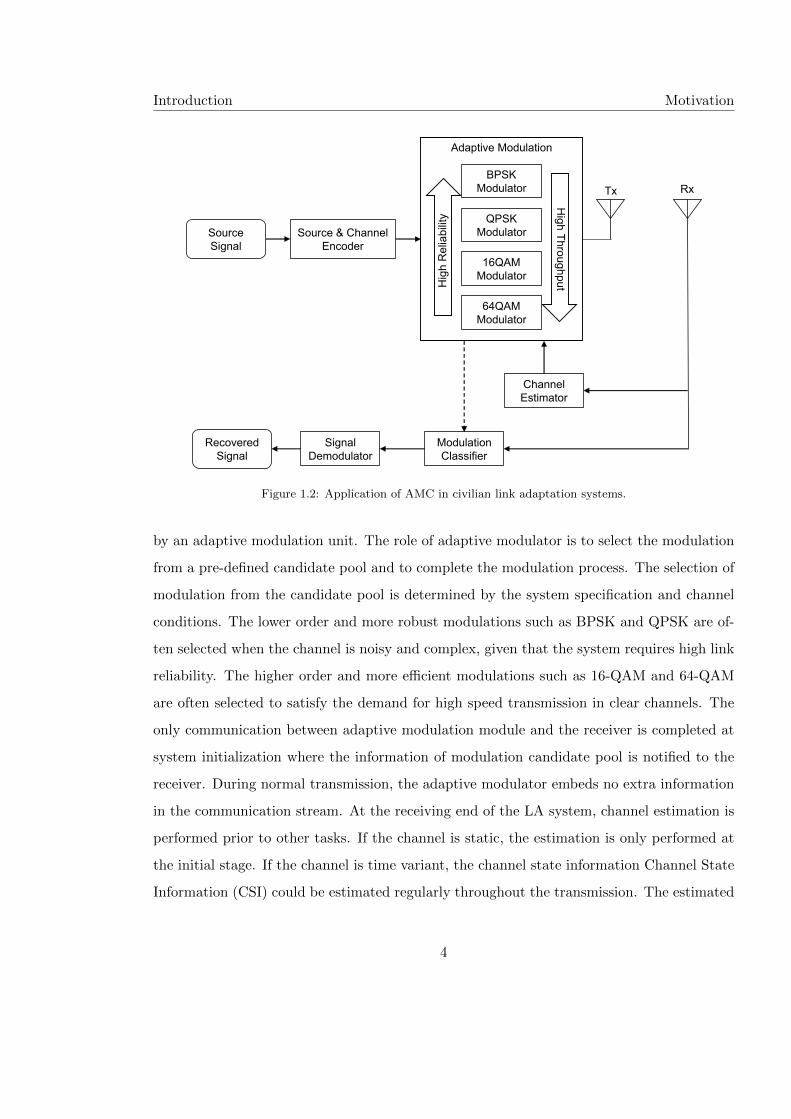
1.2 Application of AMC in civilian link adaptation systems. . . . . . . . . . . . . 4
2.1 Decision tree for signal spectral based features. . . . . . . . . . . . . . . . . . 30
3.1 Feature space and SVM with linear kernel and X1 and X2 representing two
separate feature dimensions. . . . . . . . . . . . . . . . . . . . . . . . . . . . . 39
3.2 Crossover operation in genetic algorithm. . . . . . . . . . . . . . . . . . . . . 43
3.3 Mutation operation in genetic algorithm. . . . . . . . . . . . . . . . . . . . . . 43
3.4 Genetic programming individuals in the form of a tree structure. . . . . . . . 45
3.5 Parents selected for crossover operation in genetic programming. . . . . . . . 46
3.6 Children produced by the crossover operation in genetic programming. . . . . 46
3.7 Parent selected for mutation operation and a randomly generated branch. . . 47
3.8 Two stage classification of BPSK, QPSK, 16-QAM and 64-QAM signals. . . . 50
3.9 New GP feature space for stage 1 of the GP-KNN classifier. . . . . . . . . . . 50
3.10 New GP feature space for stage 2 of the GP-KNN classifier. . . . . . . . . . . 51
3.11 Parent selected for mutation operation and a randomly generated branch. . . 54
3.12 Classification accuracy of 16-QAM and 64-QAM using GP-KNN in AWGN
channels. . . . . . . . . . . . . . . . . . . . . . . . . . . . . . . . . . . . . . . 55
3.13 Standard deviations of classification accuracy for 16-QAM and 64-QAM using
GP-KNN in AWGN channels. . . . . . . . . . . . . . . . . . . . . . . . . . . . 56
3.14 Performance comparison of GP-KNN and other methods in AWGN channels. 56
vi
4.1 Two stage classification strategy in the ODST classifier. . . . . . . . . . . . . 61
4.2 (A) 500 signal samples from 16-QAM at 15 dB, (B) 500 signal samples from
64-QAM at 15 dB, (C) The CDFs from 16-QAM and 64-QAM, and (D) The
difference between the two CDFs. The dashed lines indicate the shared opti-
mized sampling locations. . . . . . . . . . . . . . . . . . . . . . . . . . . . . . 63
4.3 Two stage classification strategy in the ODST classifier. . . . . . . . . . . . . 66
4.4 Classification accuracy of 4-QAM, 16-QAM and 64-QAM using ODST in
AWGN channel. . . . . . . . . . . . . . . . . . . . . . . . . . . . . . . . . . . 69
4.5 Classification accuracy of 4-QAM, 16-QAM and 64-QAM using ODST in
AWGN channel with different signal length. . . . . . . . . . . . . . . . . . . . 70
4.6 Classification accuracy of 4-QAM, 16-QAM and 64-QAM using GA and ODST
in AWGN channel. . . . . . . . . . . . . . . . . . . . . . . . . . . . . . . . . . 74
4.7 Classification accuracy of 4-QAM, 16-QAM and 64-QAM using ODST in fad-
ing channels with phase offsets. . . . . . . . . . . . . . . . . . . . . . . . . . . 75
4.8 Classification accuracy of 4-QAM, 16-QAM and 64-QAM using ODST in fad-
ing channels with frequency offsets. . . . . . . . . . . . . . . . . . . . . . . . . 77
4.9 Using distribution based features for AMC in two stages. . . . . . . . . . . . 81
4.10 Cumulative Distributions of different signal segments from 4-QAM and 16-
QAM at SNR of 15 dB. . . . . . . . . . . . . . . . . . . . . . . . . . . . . . . 83
4.11 Enhanced distribution based features and their distribution projection on each
separate dimension. . . . . . . . . . . . . . . . . . . . . . . . . . . . . . . . . . 87
4.12 Reference samples in new distribution based feature space. . . . . . . . . . . . 88
4.13 Classification accuracy using distribution based features in AWGN channel. . 90
4.14 Averaged classification accuracy using different classifiers in AWGN channel. 91
4.15 Averaged classification accuracy using different classifier in fading channel
carrier phase offset . . . . . . . . . . . . . . . . . . . . . . . . . . . . . . . . . 92
5.1 Implementation of blind modulation classification with minimum distance cen-
troid estimator and non-parametric likelihood function. . . . . . . . . . . . . 96
vii
5.2 Theoretical values of centroid factors A for 16-QAM and 64-QAM with differ-
ent noise levels and their analytical estimation using proposed blind centroid
estimator. . . . . . . . . . . . . . . . . . . . . . . . . . . . . . . . . . . . . . . 100
5.3 Automatic Segmentation for carrier phase offset compensation. . . . . . . . . 101
5.4 Automatic Constellation Grid Segmentation for centroid estimation. . . . . . 102
5.5 Carrier phase offset estimation and compensation for constellation grid seg-
mentation. . . . . . . . . . . . . . . . . . . . . . . . . . . . . . . . . . . . . . . 105
5.6 Error of channel gain estimation for different modulations using minimum
distance centroid estimation. . . . . . . . . . . . . . . . . . . . . . . . . . . . 108
5.7 Error of carrier phase estimation for different modulations using minimum
distance centroid estimation. . . . . . . . . . . . . . . . . . . . . . . . . . . . 109
5.8 Classification accuracy using differen classifiers in AWGN channel. . . . . . . 115
5.9 Classification accuracy using different classifiers in AWGN channel with dif-
ferent signal length. . . . . . . . . . . . . . . . . . . . . . . . . . . . . . . . . 116
5.10 Classification accuracy of using different classifiers in fading channel with slow
phase offset. . . . . . . . . . . . . . . . . . . . . . . . . . . . . . . . . . . . . . 118
5.11 Classification accuracy using different classifiers fading channel with fast phase
offset. . . . . . . . . . . . . . . . . . . . . . . . . . . . . . . . . . . . . . . . . 119
5.12 Classification accuracy using different classifiers in fading channel with fre-
quency offset. . . . . . . . . . . . . . . . . . . . . . . . . . . . . . . . . . . . . 120
5.13 Classification accuracy using different classifiers in non-Gaussian channels. . . 121
6.1 Classification accuracy of BPSK signals using the proposed blind MIMO clas-
sifier in Rayleigh fading channels. . . . . . . . . . . . . . . . . . . . . . . . . . 132
6.2 Classification accuracy of QPSK signals using the proposed blind MIMO clas-
sifier in Rayleigh fading channels. . . . . . . . . . . . . . . . . . . . . . . . . . 132
6.3 Classification accuracy of 16QAM signals using the proposed blind MIMO
classifier in Rayleigh fading channels. . . . . . . . . . . . . . . . . . . . . . . . 133
viii

6.4 Classification accuracy of BPSK signals using the proposed blind MIMO clas-
sifier in Rayleigh fading channels with varying signal length. . . . . . . . . . . 134
6.5 Classification accuracy of QPSK signals using the proposed blind MIMO clas-
sifier in Rayleigh fading channels with varying signal length. . . . . . . . . . . 135
6.6 Classification accuracy of 16QAM signals using the proposed blind MIMO
classifier in Rayleigh fading channels with varying signal length. . . . . . . . . 135
ix

List of Tables
2.1 Decision tree for modulations classification using spectral based features . . . 32
3.1 Modulation classification performance of a KNN classifier in AWGN channels 38
3.2 Parameters used in genetic programming and KNN classifier. . . . . . . . . . 51
3.3 Classification performance of a GP-KNN classifier in AWGN channels . . . . 52
3.4 Classification confusion matrix of a GP-KNN classifier in AWGN channels . . 53
3.5 Range of new GP generated feature values for different modulations between
2 dB and 5 dB. . . . . . . . . . . . . . . . . . . . . . . . . . . . . . . . . . . . 53
4.1 Parameters for the Genetic Algorithm . . . . . . . . . . . . . . . . . . . . . . 67
4.2 Classification accuracy with standard deviation of 4-QAM, 16-QAM, and 64-
QAM using ODST in AWGN channel. . . . . . . . . . . . . . . . . . . . . . . 71
4.3 Performance comparison between ODST and existing methods. . . . . . . . . 73
4.4 Complexity comparison between ODST and existing methods. . . . . . . . . . 79
4.5 Parameters used in the distribution based features classifier. . . . . . . . . . . 84
5.1 Experiment settings used to validate MDCE and NPLF classifier. . . . . . . . 112
5.2 Classification confusion matrix using the NPLF classifier in AWGN channel
with SNR=10 dB. . . . . . . . . . . . . . . . . . . . . . . . . . . . . . . . . . 114
5.3 Classification accuracy over 100 runs at every combination of SNR and Signal
Length using the NPLF classifiers. . . . . . . . . . . . . . . . . . . . . . . . . 117
5.4 Number of operators needed for different classifiers. . . . . . . . . . . . . . . . 122
x

6.1 Experiment settings for validating the blind MIMO classifier. . . . . . . . . . 131
7.1 Parameters used in the minimum distance estimator . . . . . . . . . . . . . . 153
xi
List of Symbols
α channel gain
ω additive noise
r received signal
s transmitted signal
I indicator function
F fitness functions
H Modulation Hypothesis
M modulation
M modulation pool
Σ covariance matrix
θo phase offset
A modulation alphabet
H channel coefficient
I number of modulation candidates
M modulation order/alphabet size/number of symbol states
xii

N number of sample/signal length
Pcc Classification accuracy
xiii
Acronyms
AMC Automatic Modulation Classification
ANN Artificial Neural Network
ALRT Average Likelihood Ratio Test
CDF Cumulative Distribution Function
CSI Channel State Information
EA Electronic Attack
ECDF Empirical Cumulative Distribution Function
ECM Expectation Conditional Maximization
EM Expectation Maximization
EP Electronic Protect
ES Electronic Support
EW Electronic Warfare
GA Genetic Algorithm
GLRT General Likelihood Ratio Test
GMM Gaussian Mixture Model
GoF Goodness of Fit
GP Genetic Programming
HLRT Hybrid Likelihood Ratio Test
HOS High Order Statistics
ICA Independent Component Analysis
xiv

KS test Kolmogorov-Smirnov test
KNN K-nearest Neighbour
LA Link Adaptation
LB Likelihood Based
LR Logistic Regression
MDCE Minimum Distance Centroid Estimator
MIMO Multiple-input Multiple-output
ML Machine Learning
NPLF Non-parametric Likelihood Function
ODST Optimized Distribution Sampling Test
PDF Probability Density Function
SISO Single-input Single-output
SM Spatial Multiplexing
STC Space-time Coding
SVM Support Vector Machine
xv

Acknowledgments
First and foremost, I would like to thank my parents for their endless and unconditional
support. Equally, if not more, I am grateful for the guidance provided by my primary
supervisor Prof. Asoke K. Nandi. Without his patient supervision, none of my research
outcomes would be possible. Same acknowledgement should be given to Dr. Hongying Meng
and Dr. Waleed Al-Nauimy as my secondary supervisors.
In the meantime, I owe much to my colleagues who have provided me companionship,
motivation, and inspiration. Especially to Dr. Muhammad Waqar Aslam, whom I have
extended and fruitful collaboration with. My gratitude also goes to Dr. Elsayed E. Azzouz
and Dr. M. L. Dennis Wong whose work has greatly inspired my research.
I would also like to acknowledge the financial support from th School of Engineering and
Design Brunel University London, th Faculty of Engineering University of Liverpool, and
the University of Liverpool Graduate Association (Hong Kong). The funding has helped me
focus on my research and made it possible for me to attend conferences which has much
benefited my work.
Last but not least, I would like to thank the researchers who have reviewed and provided
valuable feedback on my work. It is with your help that I am able to gauge the quality of
my work and make progress to improve.
xvi

Copyright
The author reserves other publication rights, and neither the thesis nor extensive extracts
from it may be printed or otherwise reproduced without the authors written permission. The
author attests that permission has been obtained for the use of any copyrighted material
appearing in this thesis and that all such use is clearly acknowledged.
xvii

This thesis is dedicated to my parents Qiaonan Zhu and Xiaoyan Zhu.
xviii

Chapter 1
Introduction
1.1 Motivation
1.1.1 Military applications
Automatic Modulation Classification (AMC) was first motivated by its application in military
scenarios where electronic warfare, surveillance and threat analysis requires the recognition
of signal modulations in order to identify adversary transmitting units, to prepare jamming
signals and to recover the intercepted signal. The term automatic is used as opposed to
the initial implementation of manual modulation classification where signals are processed
by engineers with the aid of signal observation and processing equipment. Most modulation
classifiers developed in the past 20 years are implemented through electronic processors.
There are three components in Electronic Warfare (EW) namely Electronic Support (ES),
Electronic Attack (EA), and Electronic Protect (EP) (Poisel, 2008). For ES, the goal is to
gather information from radio frequency emissions. This is often where AMC is employed
after the signal detection is successfully achieved. The resulting modulation information
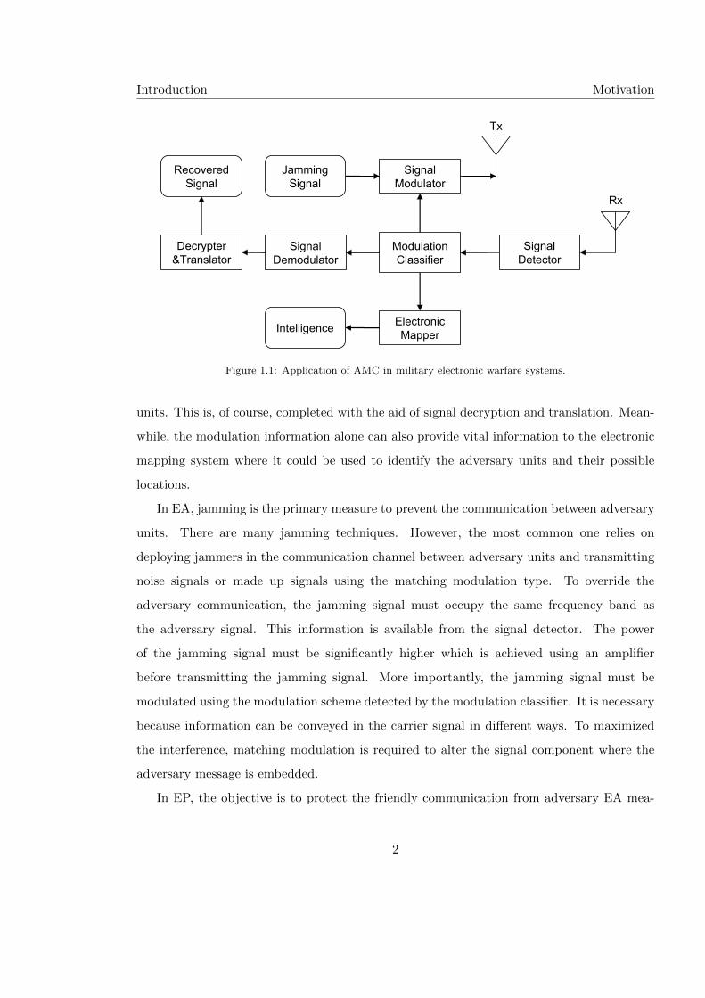
could have several uses extending into all the components in EW. An illustration of how a
modulation classifier is incorporated in the military EW systems is given in Figure 1.1.
To further the process of ES, the modulation information can be used for demodulat-
ing the intercepted signal in order to recover the transmitted message among adversary
1
Introduction Motivation
SignalModulator
Signal Detector
JammingSignal
Tx
Rx
Modulation Classifier
Signal Demodulator
Decrypter&Translator
RecoveredSignal
ElectronicMapper
Intelligence
Figure 1.1: Application of AMC in military electronic warfare systems.
units. This is, of course, completed with the aid of signal decryption and translation. Mean-
while, the modulation information alone can also provide vital information to the electronic
mapping system where it could be used to identify the adversary units and their possible
locations.
In EA, jamming is the primary measure to prevent the communication between adversary
units. There are many jamming techniques. However, the most common one relies on
deploying jammers in the communication channel between adversary units and transmitting
noise signals or made up signals using the matching modulation type. To override the
adversary communication, the jamming signal must occupy the same frequency band as
the adversary signal. This information is available from the signal detector. The power
of the jamming signal must be significantly higher which is achieved using an amplifier
before transmitting the jamming signal. More importantly, the jamming signal must be
modulated using the modulation scheme detected by the modulation classifier. It is necessary
because information can be conveyed in the carrier signal in different ways. To maximized
the interference, matching modulation is required to alter the signal component where the
adversary message is embedded.
In EP, the objective is to protect the friendly communication from adversary EA mea-
2

Introduction Motivation
sures. As mentioned above, jammers transmit higher power signals to override adversary
communication in the same frequency band. The key is to have the same signal modulation.
An effective strategy to prevent friend communication being jammed is to have awareness
of the EA effort from adversary jammers and to dodge the jamming effort. More specifi-
cally, the friendly transmitter could monitor the jamming signals modulation and switch the
friendly unit to a different modulation scheme to avoid jamming.
During the 1980s and 1990s, there were considerable numbers of researchers in the field of
signal processing and communications who dedicated their works to the problem of automatic
modulation classification. It leads to the publication of the first well received book on the
subject by Azzouz and Nandi in 1996 (Azzouz and Nandi, 1996a). The interest in AMC for
military purposes is sustained till this very day.
1.1.2 Civilian applications
The beginning of 21st century sees a large number of innovations in communications technol-
ogy. Among them are a few that have made essential contributions to the staggering increase
of transmission throughput in various communication systems. Link Adaptation (LA), also
known as adaptive modulation and coding, creates an adaptive modulation scheme where a
pool of multiple modulations are employed by the same system (Goldsmith and Chua, 1998).
It enables the optimizing of the transmission reliability and data rate through the adaptive
selection of modulation schemes according to channel conditions. While the transmitter has
the freedom to choose how the signals are modulated, the receiver must have the knowledge
of the modulation type to demodulate the signal so that the transmission could be successful.
An easy way to achieve this is to include the modulation information in each signal frame
so that the receivers would be notified about the change in modulation scheme and react
accordingly. However, this strategy affects the spectrum efficiency due to the extra modu-
lation information in each signal frame. In the current situation where wireless spectrum is
extremely limited and valuable, the aforementioned strategy is simply not efficient enough.
For this reason, AMC becomes an attractive solution to the problem.
As demonstrated in Figure 1.2, the signal modulator in the LA transmitter is replaced
3
Introduction Motivation
SourceSignal
Tx Rx
Source fpChannelpEncoder
BPSKModulator
QPSKModulator
16QAMModulator
64QAMModulator
HighpT
hroughputH
ighp
Rel
iabi
lity
AdaptivepModulation
ChannelpEstimator
ModulationClassifier
SignalDemodulator
RecoveredSignal
Figure 1.2: Application of AMC in civilian link adaptation systems.
by an adaptive modulation unit. The role of adaptive modulator is to select the modulation
from a pre-defined candidate pool and to complete the modulation process. The selection of
modulation from the candidate pool is determined by the system specification and channel
conditions. The lower order and more robust modulations such as BPSK and QPSK are of-
ten selected when the channel is noisy and complex, given that the system requires high link
reliability. The higher order and more efficient modulations such as 16-QAM and 64-QAM
are often selected to satisfy the demand for high speed transmission in clear channels. The
only communication between adaptive modulation module and the receiver is completed at
system initialization where the information of modulation candidate pool is notified to the
receiver. During normal transmission, the adaptive modulator embeds no extra information
in the communication stream. At the receiving end of the LA system, channel estimation is
performed prior to other tasks. If the channel is static, the estimation is only performed at
the initial stage. If the channel is time variant, the channel state information Channel State
Information (CSI) could be estimated regularly throughout the transmission. The estimated
4
Introduction Problem statement
CSI and other information would then be feedback to the transmitter where the CSI will be
used for the selection of modulation schemes. More importantly, the CSI is required to assist
the modulation classifier. Depending on the AMC algorithm, different channel parameters
are needed to complete modulation classification. Normally the accuracy of channel estima-
tion has a significant impact on the performance of the modulation classifier. The resulting
modulation classification decision is then fed to the reconfigurable signal demodulator for
appropriate demodulation. If the modulation classification is accurate, the correct demodu-
lation method would capture the message and complete the successful transmission. If the
modulation classification is incorrect, the entire transmission fails as the message cannot be
recovered from the demodulator. It is not difficult to see the importance of AMC in LA
systems.
Thanks to the development in microprocessors, receivers nowadays are much more able in
terms of their computational power. Thus, the signal processing required by AMC algorithms
becomes feasible. By automatically identifying the modulation type of the received signal,
the receiver does not need to be notified about the modulation type and the demodulation
can still be successfully achieved. In the end, the spectrum efficiency is improved as no
modulation information is needed in the transmitted signal frame. AMC has become an
integral part of the intelligent radio systems including cognitive radio and software defined
radio.
1.2 Problem statement
Assuming there is a finite set of modulation candidates, the modulation pool M consists of
I number of candidate modulations with M(i) being the ith modulation candidate. The
transmitted signal s consisting of N samples is modulated usingM which is unknown to the
receiver. For each digital modulation scheme, the transmitted signal samples are mapped
from a unique set of symbol alphabet dictated by the modulation scheme. The received
signal r = Hs + ω is the main or sometime sole subject for analysis where H is associated
with different channel effects and ω is the additive noise. The task of AMC is to find
5
Introduction Summary of contributions
the modulation candidate from the modulation pool which matches the actual modulation
scheme used for the signal transmission. The criteria for a good modulation classifier are
based on four aspects.
First, a modulation classifier should be able to classify as many modulation types as
possible. Such a trait makes a modulation classifier easily applicable to different applications
without needing any modification to accommodate extra modulations. Second, a modulation
classifier should provide high classification accuracy. The high classification accuracy is
relative to different noise levels. Third, the modulation classifier should be robust for many
different channel conditions. The robustness can be provided by either the built in channel
estimation and compensation mechanism or the natural resilience of the modulation classifier
against channel conditions. Fourth, the modulation classifier should be computationally
efficient. In many applications, there is a strict limitation on computation power which may
be unsuitable for over complicated algorithms. Meanwhile, some applications may require
fast decision making which demands the classification to be completed in real time. Only a
modulation classifier with high computational efficiency could meet this requirement. After
all, a simple and fast modulation classifier algorithm is always appreciated.
In practice, there is no one classifier that is perfect in all aspects. Therefore, the goal of
this research is to develop different AMC strategies that excel in certain aspects with reason-
able compromise in other departments. The significance of these different AMC strategies
is accentuated by the wide variety of applications which demand a unique set of attributes
from the classifier.
1.3 Summary of contributions
As of this stage, I believe that the following contributions to the field has been achieved
through this project:
• Machine Learning (ML) algorithms are introduced to feature based modulation classi-
fication strategy. The machine learning based classifiers incorporate logistic regression,
genetic algorithm, or genetic programming as feature selection/combination methods
6
Introduction Thesis organization
and k-nearest neighbour or support vector machine as classifiers. The machine learn-
ing based classifiers are proven to be more intuitive in their implementation and more
accurate than the traditional feature based classifiers. (Chapter 3)
• Empirical cumulative distribution of modulation signals are studied to suggest distri-
bution test based modulation classifiers as well as distribution statistics that can be
used as features. The distribution based modulation classification approaches have
very low computational complexity while preserving high classification accuracy when
limited number of signal samples are available for analysis.(Chapter 4)
• Thus far, noise models are always assumed when constructing a modulation classifier.
In this research, the blind modulation classifier which operates without an assumed
noise model is developed using a centroid estimator and a Non-parametric Likelihood
Function (NPLF). The combination provides improved robustness in fading channels
as well as superior classification performance with impulsive noises. (Chapter 5)
• The combination of expectation maximization (EM) estimator and maximum likeli-
hood classifier is extended to the Multiple-input Multiple-output (MIMO) systems.
Oppose to Independent Component Analysis (ICA) enabled MIMO modulation clas-
sifier, the EM and ML combination doesn’t require the knowledge of noise power or
extra calculation for phase offset correction. (Chapter 6)
1.4 Thesis organization
This thesis begins with a brief introduction to the subject, some basic theories, and a lit-
erature review. The following contents include different modulation classifiers developed in
this research presented in chronological order. The thesis is concluded with a review of the
developed classifiers and suggestions for further research direction. The summary of each
chapter is given below.
Chapter 1 provides the historical background of AMC as well as its important appli-
cations in military and modern civilian communication systems. The contribution of this
7

Introduction Thesis organization
research is highlighted with complimentary list of publications.
Chapter 2 provides the modelling of communication systems and different communica-
tion channels that are used for the development of modulation classifiers. The scope of the
research and assumptions made are described. A literature review is included to provide an
understanding of the development progress of AMC at the current stage. Three of the state-
of-the-art algorithms are described in details as they are used in performance benchmarking
versus the newly developed algorithms in this research.
Chapter 3 lists several machine learning techniques that have been introduced to AMC
(Zhu et al., 2011, 2013c, 2014; Aslam et al., 2012). K-nearest neighbour and support vector
machine are suggested as classifiers based on high order statistics features. Feature selection
and combination are practised using logistic regression, genetic algorithm, and genetic pro-
gramming. The combination of these classifiers and feature enhancement methods are also
discussed to provide a complete solution to AMC. For each algorithm, its implementation
is described in details. The advantages and disadvantages of each algorithm are listed with
numerical results to support the observation.
Chapter 4 explores the AMC algorithms based on signal distributions (Zhu et al., 2013c,
2014). The optimized distribution sampling test is suggested as an improved version of
the Kolmogorov-Smirnov test. The strategies of optimizing the sampling locations and the
distribution test as classifier are described in detail. The additional use of sample distribution
statistics as features is explored for AMC accompanied with ML classifiers. The numerical
results from computer aided simulations are provided to validate the proposed methods.
Chapter 5 describes the new AMC solution which does not require known noise model
(Zhu et al., 2013b; Zhu and Nandi, 2014a). The preliminary step of centroid estimation can
be achieved through two iterative algorithms. The likelihood based modulation classification
is realized by a non-parametric likelihood function. The theoretical analysis is given for the
validation of the centroid estimator and the optimization of the NPLF classifier. Numerical
results are given to illustrate the superior performance of this classifier in complex channels.
Chapter 6 gives the blind modulation classification solution for MIMO systems (Zhu and
Nandi, 2014b). The joint estimation of channel matrix and noise variance is achieved with
8
Introduction List of publications
expectation maximization in the context of MIMO channels. The expectation/conditional
maximization update functions for the channel parameters are derived. The classification
is completed with a ML classifier and updated likelihood functions for MIMO signals. The
simulated classification performance is given for several selected modulations.
Chapter 7 reviews the new classifiers developed in this research and concludes their
advantages and disadvantages. The remaining challenges and new directions for the subject
is also listed in this chapter.
1.5 List of publications
Journal Papers
• Zhu, Z., and Nandi, A. K. (2014). Blind Digital Modulation Classification using Min-
imum Distance Centroid Estimator and Non-parametric Likelihood Function. IEEE
Transactions on Wireless Communications, 13(8) 4483-4494.
• Zhu, Z., Aslam, M. W., and Nandi, A. K. (2014). Genetic Algorithm Optimized
Distribution Sampling Test for M-QAM Modulation Classification. Signal Processing,
94, 264-277.
• Aslam, M. W., Zhu, Z., and Nandi, A. K. (2013). Feature generation using genetic
programming with comparative partner selection for diabetes classification. Expert
Systems with Applications, 40(13), 5402-5412.
• Aslam, M. W., Zhu, Z., and Nandi, A. K. (2012). Automatic Modulation Classification
Using Combination of Genetic Programming and KNN. IEEE Transactions on Wireless
Communications, 11(8), 2742-2750.
Conference papers
• Zhu, Z., and Nandi, A. K. (2014). Blind Modulation Classification for MIMO Systems
using Expectation Maximization. In Military Communications Conference (pp. 1-6).
9

Introduction List of publications
• Zhu, Z., Nandi, A. K., and Aslam, M. W. (2013). Approximate Centroid Estimation
with Constellation Grid Segmentation for Blind M-QAM Classification. In Military
Communications Conference (pp. 46-51).
• Zhu, Z., Aslam, M. W., and Nandi, A. K. (2013). Adapted Geometric Semantic Genetic
Programming for Diabetes and Breast Cancer Classification. In IEEE International
Workshop on Machine Learning for Signal Processing (pp. 1-5).
• Aslam, M. W., Zhu, Z., and Nandi, A. K. (2013). Improved Comparative Partner
Selection with Brood Recombination for Genetic Programming. In IEEE International
Workshop on Machine Learning for Signal Processing (pp. 1-5).
• Zhu, Z., Nandi, A. K., and Aslam, M. W. (2013). Robustness Enhancement of Distri-
bution Based Binary Discriminative Features for Modulation Classification. In IEEE
International Workshop on Machine Learning for Signal Processing (pp. 1-6).
• Zhu, Z., Aslam, M. W., and Nandi, A. K. (2011). Support Vector Machine Assisted Ge-
netic Programming for MQAM Classification. In International Symposium on Signals,
Circuits and Systems (pp. 1-6).
• Aslam, M. W., Zhu, Z., and Nandi, A. K. (2011). Robust QAM Classification Using
Genetic Programming and Fisher Criterion. In European Signal Processing Conference
(pp. 995-999).
• Zhu, Z., Aslam, M. W., and Nandi, A. K. (2010). Augmented Genetic Programming
for Automatic Digital Modulation Classification. In IEEE International Workshop on
Machine Learning for Signal Processing (pp. 391-396).
• Aslam, M. W., Zhu, Z., and Nandi, A. K. (2010). Automatic Digital Modulation Clas-
sification Using Genetic Programming with K-Nearest Neighbor. In Military Commu-
nications Conference (pp. 1731-1736).
10
Chapter 2
Signal Model and Existing Methods
2.1 Introduction
Signal models are the starting point of every meaningful modulation classification strategy.
Algorithms such as likelihood based, distribution test based and feature based classifiers all
require an established signal model to derive the corresponding rules for classification decision
making. While some unsupervised machine learning algorithms could function without a
reference signal model, the optimization of such algorithms still relies on the knowledge of a
known signal model. Meanwhile, as the validation of modulation classifiers is often realized
by computer-aided simulation, accurate signal modelling provides meaningful scenarios for
evaluating the performance of various modulation classifiers. The objective of this chapter is
to establish some unified signal models for different modulation classifiers listed in Chapter
3 to Chapter 6. Through the process, the accuracy of the models will be the first priority.
That, however, is with a fine balance of simplicity in the models to enable theoretical analysis
and to provide computational efficient implementations. Signal models are presented in three
different channels namely AWGN channel, fading channel, and non-Gaussian channel.
To establish an understanding of the current AMC development status, a literature review
of some the key existing methods is also included in this chapter. Three major categories
of classifiers are visited including likelihood based classifiers, distribution test based clas-
sifiers and feature based classifiers. For some classifiers that are used in the performance
11
Signal Model and Existing Methods Signal Model in AWGN channels
benchmarking, their implementation is describe in details.
2.2 Signal model in AWGN channels
Additive white Gaussian noise is one of the most widely used noise models in many signal
processing problems. It is of much relevance to the transmission of signals in both wired
and wireless communication media where wideband Gaussian noise is produced by thermal
vibration in conductors and radiation from various sources. The popularity of additive
white Gaussian noise is evidential in most published literature on modulation classification
where the noise (model) is considered the fundamental limitation to accurate modulation
classification.
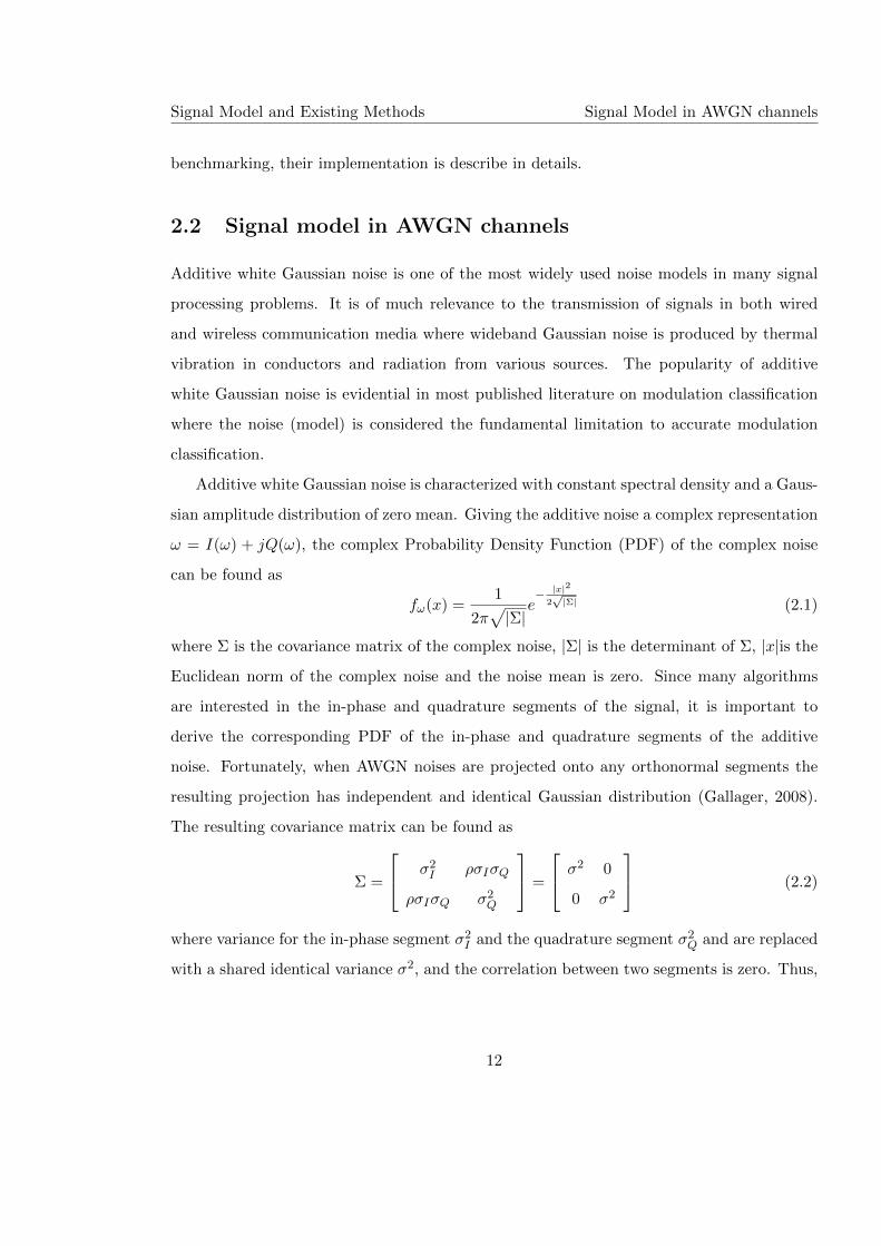
Additive white Gaussian noise is characterized with constant spectral density and a Gaus-
sian amplitude distribution of zero mean. Giving the additive noise a complex representation
ω = I(ω) + jQ(ω), the complex Probability Density Function (PDF) of the complex noise
can be found as
fω(x) =1
2π√|Σ|
e− |x|2
2√|Σ| (2.1)
where Σ is the covariance matrix of the complex noise, |Σ| is the determinant of Σ, |x|is the
Euclidean norm of the complex noise and the noise mean is zero. Since many algorithms
are interested in the in-phase and quadrature segments of the signal, it is important to
derive the corresponding PDF of the in-phase and quadrature segments of the additive
noise. Fortunately, when AWGN noises are projected onto any orthonormal segments the
resulting projection has independent and identical Gaussian distribution (Gallager, 2008).
The resulting covariance matrix can be found as
Σ =
σ2I ρσIσQ
ρσIσQ σ2Q
=
σ2 0
0 σ2
(2.2)
where variance for the in-phase segment σ2I and the quadrature segment σ2
Q and are replaced
with a shared identical variance σ2, and the correlation between two segments is zero. Thus,
12
Signal Model and Existing Methods Signal model in fading channels
the desired PDFs of each segment can be easily derived as
fI(ω)(x) = fQ(ω)(x) =1
σ√
2πe−|x|2
2σ2 (2.3)
As suggested by the term “additive”, the AWGN noise is added to the transmitted signal
giving the signal model in AWGN channel.
r(t) = s(t) + ω(t). (2.4)
Assuming the signal modulation M has an alphabet A of M symbols and the symbol Am
having the equal probability to be transmitted, with overall distribution being considered
as M number of AWGN noise distributions shifted to different modulation symbols, the
complex PDF of the received signal is given by
fr(x) =M∑m=1
1
Mfω(x|Am,Σ) =
M∑m=1
1
M
1
2π√|Σ|
e− |x−Am|
2
2√|Σ| (2.5)
where 1/M is the probability of Am being transmitted.
Following the same logic of the derivation of the complex PDF, the distribution of received
signals on their in-phase and quadrature segments can be found by replacing the variance by
half of the noise variance and the mean of the noise distribution with in-phase and quadrature
segments of the modulation symbols.
fI(r)(x) =
M∑m=1
1
MfI(ω)(x|Am, σ) =
M∑m=1
1
M
1
σ√
2πe−|x−I(Am)|2
2σ2 (2.6)
2.3 Signal model in fading channels
The fading channel is largely concerned with wireless communication, where signals are
received as delayed and attenuated copies after being absorbed, reflected and diffracted
by different objects. Fading, especially deep fading, drastically changes the property of the
transmitted signal and imposes a tough challenge on the robustness of a modulation classifier.
Though early literature on modulation classifier focuses on the validation of algorithms
in AWGN channel, the current standard requires the robustness in fading channel as an
important attribute In this chapter, a unified model of a fading channel is presented with
13

Signal Model and Existing Methods Signal model in fading channels
flexible representation of different fading scenarios. It is worth noting that AWGN noise will
also be considered in the fading channel as to approach a more realistic real world channel
condition.
Instead of modelling each fading type, we characterize the joint effect of them into three
categories: attenuation, phase offset, and frequency offset. Depending on the nature of the
fading channel, two types of fading scenarios are generally considered for signal phase offset:
slow fading and fast fading. Slow fading are normally caused by shadowing (or shadow
fading) when the signal is obscured by large object from a line of sight communication
(Goldsmith, 2005). As the coherent time of the shadow fading channel is significantly longer
than the signal period, the effect of attenuation and phase offset remains constant. Therefore,
a constant channel gain α and phase offset θo can be used to model the received signal after
slow fading.
r(t) = αejθos(t) + ω(t) (2.7)
Fast fading, caused by multipath fading where signals are reflected by objects in the radio
channel of different properties, imposes a much different effect on the transmitted signal.
As the coherent channel time in a fast fading channel is considered small. The effects
of attenuation and phase offset vary with time. In this research, we assume that both
the attenuation and phase offset are random processes with Gaussian distributions. The
attenuation is given by
α(t) ∼ N (α, σα) (2.8)
where α(t) is the channel gain at time t, α is the mean attenuation, and σα is the variance
of the channel gain. The phase offset is given by
θo(t) ∼ N (θo, σθo) (2.9)
where θo(t) is the channel gain at time t, θo is the mean attenuation, and σθo is the variance
of the channel gain. Both expressions give a combined effect of slow and fast fading. When α
and θo are both zero, the fading consist of only fast attenuation and fast phase offset. When
σα and σθo are both zero, the model reverts back to the case of slow fading. The resulting
14
Signal Model and Existing Methods Signal model in non-Gaussian channels
channel model becomes
r(t) = α(t)ejθo(t)s(t) + ω(t). (2.10)
Apart from the channel attenuation and phase offset, frequency offset is another impor-
tant effect in a fading channel that is worth investigating. The shift in frequency of received
signal is mostly cause by moving antennas in mobile communication devices. Given the car-
rier frequency of a modulated signal as fc, when the antenna is moving at a speed of v the
resulting frequency offset caused by Doppler shift can be found as fcv/c where c is the speed
of travelling light in the channel medium (Gallager, 2008). As we are only interested in the
amount of frequency offset, the expression is simplified by denoting the frequency offset set
as fo and the resulting signal model with frequency offset set given by
r(t) = ej2πtfos(t) + ω(t) (2.11)
Combining the attenuation, phase offset, and frequency offset, we can derive a signal
model of fading channel of all mentions effects.
r(t) = α(t)ej(2πtfo+θo(t))s(t) + ω(t) (2.12)
2.4 Signal model in non-Gaussian channels
Non-Gaussian noises are often used to model impulsive noises which are a step further to
model the noises in a real radio communication channel. Impulsive noise, unlike Gaussian
noise, has heavy-tailed probability density function meaning higher probability for high power
noise components. Such noises are often the result of incidental electromagnetic radiation
from man-made sources. While not featured in most modulation classification literature,
impulsive noises have received increasing amount of attention in recent years. Despite the
complexity in the modelling of impulsive noise, it is worth the effort to try and accommodate
the signal model for a more practical approximation of the real world radio channels. In this
chapter, two non-Gaussian noise models will be presented for modelling the impulsive noise.
However, such noises will be considered solely without extra AWGN noise or fading effects.
15

Signal Model and Existing Methods Signal model in non-Gaussian channels
In this section, we start with Middleton’s class A non-Gaussian noise model as a complex
but accurate modelling of impulsive noises. In addition, the Gaussian mixture model is
established for the analytical convenience in some of the complex modulation classification
algorithms. The subject of non-Gaussian noise in AMC has been studied by Chavali and
Silva extensively (Chavali and da Silva, 2011, 2013).
Middleton proposed a series of noise models (Middleton, 1999) to approximate the impul-
sive noise generated by different natural and man-made electromagnetic activities in physical
environments. These models have become popular in many fields, including wireless commu-
nication, thanks to the canonical nature of the model which is invariant of the noise sauce,
noise waveform, and propagation environments. The versatility of the model is enhanced by
the model parameters which provide possibility to specify the source distribution, propaga-
tion properties, and bean patterns. The class A model is defined for the non-Gaussian noises
with bandwidth narrower than the receiver bandwidth, while the class B model is defined
for the non-Gaussian noises with wider spectrum than the receiver. In the meantime, the
class C model provides a combination of the class A and class B model. The PDF of the
class A noise is derived as
fω(x) = e−AA∞∑k=0
AkA
k!√
4πσ2kA
e− x2
4πσ2kA (2.13)
where AA is the overlap index which defines the number of noise emissions per second times
the mean duration of the typical emission (Middleton, 1999). The variance of the kth emission
element is given by
2σ2kA =
kAA
+ ΓA
1 + ΓA(2.14)
where ΓA is the Gaussian factor defined by the ratio of the average power of the Gaussian
component to the average power of the non-Gaussian components. To approximate the de-
sired impulsive nature in this section, small overlap index and Gaussian factor are suggested
to provide a heavy-tailed distribution for the noise simulation.
In the meantime, Vastola proposed to approximate the Middletons class A model through
a mixture of Gaussian noises (Vastola, 1984). The conclusion was drawn that the Gaussian
16
Signal Model and Existing Methods Likelihood based classifiers
Mixture Model (GMM) provides a close approximation to the Millertons class A model while
being computationally much more efficient. The PDF of the GMM mode is given by
fω(x) =K∑k=1
λk2πσ2
k
e− |x|
2
2σ2k (2.15)
where K is the total number of Gaussian components, λk is the probability of the noise
being chosen from the kth component, and σ2k is the variance of the kth component. As the
GMM will be used as the primary model for impulsive noise, there we derive the PDFs of
received signals in the non-Gaussian channel with a GMM noise model. Assume the GMM
uses components where the probability and variance for each component are either known
or estimated. The PDF of complex signal in the non-Gaussian channel can be derived as
fr(x) =M∑m=1
1
M
K∑k=1
fr(x|Am, λk, σk) =
M∑m=1
1
M
K∑k=1
λk2πσ2
k
e−|x−Am|2
2σ2 (2.16)
with the corresponding variation for signal I-Q segments given by
fI(r)(x) =M∑m=1
1
M
K∑k=1
fI(r)(x|Am, λk, σk) =M∑m=1
1
M
K∑k=1
λk
σk√
2πe−|x−I(Am)|2
2σ2 (2.17)
2.5 Likelihood based classifiers
Likelihood Based (LB) modulation classifiers are by far the most popular modulation clas-
sification approaches. The interest in LB classifiers is motivated by the optimality of its
classification accuracy when perfect channel model and channel parameters are known to
the classifiers. The common approach of a LB modulation classifier consists of two steps.
In the first step, the likelihood is evaluated for each modulation hypothesis with observed
signal samples. The likelihood functions are derived from the selected signal model and can
be modified to fulfil the need of reduced computational complexity or to be applicable in
non-cooperative environments. In the second step, the likelihood of different modulation
hypothesizes are compared to conclude the classification decision.
17
Signal Model and Existing Methods Likelihood based classifiers
2.5.1 Maximum likelihood classifier
Likelihood evaluation is equivalent to the calculation of probabilities of observed signal sam-
ples belonging to the models with given parameters. In a maximum likelihood classifier (Wei
and Mendel, 2000), with perfect channel knowledge, all parameters are known except the
signal modulation. Therefore, the classification process can also be perceived as a maximum
likelihood estimation of the modulation type where the modulation type is found in a finite
set of candidates. Given that the likelihood of the observed signal sample r[n] belongs to
the modulationM is equal to the probability of the signal sample r[n] being observed in the
AWGN channel modulated with M,
L(r[n]|M, σ) = p(r[n]|M, σ) (2.18)
as we recall the complex form PDF of received signal in AWGN channel, the likelihood
function can be found as
L(r[n]|M, σ) =M∑m=1
1
M
1
2πσ2e−|r[n]−Am|2
2σ2 (2.19)
Without knowing which modulation symbol the signal sample r[n] belong to, the likelihood
is calculated using the average of the likelihood value between the observed signal sample
and each modulation symbol Am. The joint likelihood given multiple observed samples is
calculated with the multiplication of all likelihood of individual samples.
L(r|M, σ) =
N∏n=1
M∑m=1
1
M
1
2πσ2e−|r[n]−Am|2
2σ2 (2.20)
For analytical convenience in many cases, the natural logarithm of the likelihood is used as
likelihood value to be compared in a maximum likelihood classifier.
logL(r|M, σ) = log
(N∏n=1
M∑m=1
1
M
1
2πσ2e−|r[n]−Am|2
2σ2
)
=N∑n=1
log
(M∑m=1
1
M
1
2πσ2e−|r[n]−Am|2
2σ2
)(2.21)
The likelihood, in the meantime, can be derived from probabilities of different aspects of
sampled signals. As we have derived the PDF for In-phase segments of received signal in
18
Signal Model and Existing Methods Likelihood based classifiers
AWGN channel, the corresponding likelihood function of the in-phase segments of a signal
can be found as
LI(r)(r|M, σ) =N∏n=1
M∑m=1
1
M
1
σ√πe−|I(r[n])−I(Am)|2
σ2 . (2.22)
Having established the likelihood functions in AWGN channel, the decision making in
a ML classifier becomes rather straightforward. Assuming a pool M with finite number
of I modulation candidates, among which hypothesis HM(i) of each modulation M(i) is
evaluated using estimated channel parameters ΘM(i) and suitable likelihood function to
obtain its likelihood evaluation L(r|HM(i)). With all the likelihood collected the decision
made simply by finding the hypothesis with the highest likelihood.
M = arg maxM(i)∈M
L(r|HM(i)) (2.23)
2.5.2 Likelihood ratio test classifier
The issue of unknown parameter in a ML classifier is pivotal as the likelihood function is
unable to handle any missing parameter. Average Likelihood Ratio Test (ALRT) is one way
to overcome such limitation of a ML classifier. Polydoros and Kim first applied ALRT on
modulation classification (Polydoros and Kim, 1990) which was later adopted by Huang and
Polydoros (Huang and Polydoros, 1995), Beidas and Weber, Sills (Sills, 1999), Hong and
Ho (Hong and Ho, 2000). Different from the ML likelihood function, the ALRT likelihood
function replaces unknown parameters with the integral of all its possible values and their
corresponding probabilities. Assuming that the channel parameters set Θ consisting channel
gain α, noise variance σ2, and phase offset θo is unknown to the classifier, the ALRT likelihood
function is given by
LALRT (r) =
∫ΘL(r|Θ)f(Θ|H)dΘ
=
∫Θ
N∏n=1
M∑m=1
1
M
1
2πσ2e−|r[n]−αe−jθoAm|2
2σ2 f(α, σ, θo|H)dΘ (2.24)
where L(r|Θ) is the likelihood given the channel parameter set Θ, f(Θ|H) is the probability
of the parameters Θ under modulation hypothesis H. The probability depends on deification
19

Signal Model and Existing Methods Likelihood based classifiers
of prior probability of the unknown parameters. The common assumption of prior PDFs of
different channel parameters are given below
f(α|H) ∼ N (α|µα, σα) (2.25)
f(σ2|H) ∼ Gamma(σ2|aσ, bσ) (2.26)
f(θo|H) ∼ N (θo|µθo , σθo) (2.27)
where channel gain α is given a normal distribution with mean µα, variance σ2α, noise variance
is given a Gamma distribution with shape parameter aσ and scale parameter bσ, and phase
offset is given a normal distribution with mean µθo and variance σ2θo
. All the additional
parameters associated with PDF of channels parameters are often called hyperparameters.
The estimation of hyperparameters is not discussed in this research. Suitable schemes have
been proposed by Roberts and Penny using variational Bayes estimator (Roberts and Penny,
2002).
The likelihood ratio test required for the classification decision making is conducted with
the assistance of a threshold γA. The actual likelihood ratio is calculated as follows
ΛA(i, j) =
∫Θ L(r|θ)f(θ|HM(i))dθ∫Θ L(r|θ)f(θ|HM(j))dθ
(2.28)
where the classification result is given using the conditional equation
M =
M(i) if ΛA(i, j) ≥ γAM(j) if ΛA(i, j) < γA
(2.29)
An easy assignment of the ratio test threshold is to define all thresholds to be one. The deci-
sion making becomes simple process of comparing the average likelihood of two hypotheses.
M =
M(i) if LALRT (r|HM(i)) ≥ LALRT (r|HM(j))
M(j) if LALRT (r|HM(i)) < LALRT (r|HM(j))(2.30)
Using the same assignment, the maximum likelihood decision making can also be applied
using (2.23) with the likelihood function with average likelihood.
It is not difficult to see that the ALRT likelihood function has a much more complex
form when unknown parameters are introduced. The requirement of underlining models
20
Signal Model and Existing Methods Likelihood based classifiers
for unknown parameters rules that successful classification depends on the accuracy of the
models. Consequently, if an accurate channel model is not known, the method becomes
suboptimal and only an approximation to the optimal ALRT classifier. The additional
requirement of the estimation hyperparameters adds yet another level of complexity and
inaccuracy to the overall performance of the ALRT classifier. This is without mentioning
that the likelihood function is more complex through an added integration operation.
For the above reason, Panagiotou, Anastasopoulos, and Polydoros proposed the General
Likelihood Ratio Test (GLRT) as an alternative (Panagiotou et al., 2000). The GLRT in
essence is a combination of a maximum likelihood estimator and a maximum likelihood
classifier. The likelihood function, unlike the ALRT, replaces the integration of unknown
parameters with a maximization of the likelihood over a possible interval for the unknown
parameters. The likelihood function of the GLRT method is given by
LGLRT (r) = maxΘL(r|α, σ, θo) = max
Θ
N∏n=1
maxAm∈A
1
M
1
2πσ2e−|r[n]−αe−jθoAm|2
2σ2 (2.31)
The complexity is notably further reduced. However, the classifier based on the modified
GLRT likelihood function now becomes biased in both low SNR and high SNR scenarios.
Assuming the modified GLRT likelihood function is used to classify among 4-QAM and
16-QAM signals. At low SNR, when signals are well spread, a 4-QAM modulated signal
is always more likelihood to produce higher likelihood to a 16-QAM symbol, because the
16-QAM has more symbols and they are more densely populated under the assumption of
unit power. At high SNR, when the signal is tight around the transmitted symbol, the max-
imization of the likelihood through channel gain is likely to be scaled the 16-QAM alphabets
so that four symbols in the alphabet will be overlapping with the alphabet of the 4-QAM
modulation. Such phenomenon observed in nested modulations produces equal likelihood
between low order modulations and high order modulations when low order modulations are
being classified. Therefore, the method is clearly biased for high order modulations in most
scenarios.
While GLRT likelihood function provides alternative to ALRT, the fact that it is a biased
classifier, as discussed in the previous section, makes it unsuitable for modulation with nested
21
Signal Model and Existing Methods Likelihood based classifiers
modulations (e.g. QPSK, 8-PSK; 16-QAM, 64-QAM). For this reason, Panagiotou et al.
proposed another likelihood ratio test named Hybrid Likelihood Ratio Test (HLRT). In the
original publication, the HLRT is suggested as a LB classifier for unknown carrier phase
offset. The likelihood in HLRT is calculated by averaging over the transmitted symbols and
then maximizing the resulting likelihood function with respect to the carrier phase. The
likelihood function is thus derived as
LHLRT (r) = maxθo∈[0,2π]
L(r|θo) = maxθo∈[0,2π]
N∏n=1
M∑m=1
1
M
1
2πσ2e−|r[n]−αe−jθoAm|2
2σ2 . (2.32)
It is clear that the HLRT likelihood function calculates the likelihood of each signal
sample belong to each alphabet symbol. Therefore, the case where a nested constellation
creates a biased classification is of no existence. In addition, the maximization process
replaces the integral of the unknown parameters and there PDFs for much lower analytical
and computational complexity.
2.6 Distribution test based classifiers
When the observed signal is of sufficient length, the empirical distribution of the modulated
signal becomes an interesting subject to study for modulation classification. In the beginning
of this chapter, the signal distributions in various channels are given. It is clear that the signal
distributions are mostly determined by two factors namely modulation symbol mapping and
channel parameters. Assuming that the channel parameters are pre-estimated and available,
the only variable in the signal distribution becomes the symbol mapping which is directly
associated with the modulation scheme.
By reconstructing the signal distribution using the empirical distribution, the observed
signals can be analysed through their signal distributions. If the theoretical distribution
of different modulation candidates is available, there will exist one which best matches the
underlying distribution of the signal to be classified. The evaluation of equality between
difference distributions is also known as Goodness of Fit (GoF) which indicates how the
sampled data fit the reference distribution. Ultimately, the classification is completed by
finding the hypothesised signal distribution that has the best goodness of fit.
22
Signal Model and Existing Methods Likelihood based classifiers
2.6.1 One-sample KS test
Kolmogorov-Smirnov test is a goodness of fit test which evaluates the equality of two proba-
bility distributions (Conover, 1980). The reference probability distributions can be sampled
or theoretical Cumulative Distribution Function (CDF). There are two types of of KS test:
one-sample KS test and two-sample test. In this section, we start with one-sample KS test
which samples only the observed signal. In the next section, the two-sample KS test which
samples both the observed signal and the reference signal is presented.
Massey first introduced the KS test (Massey 1951) building on theories developed by
Kolmogorov (Kolmogorov, 1933) and Smirnov (Smirnov, 1939). The KS test has since been
applied in many signal processing problems. F. Wang and X. Wang (Wang and Wang, 2010)
first adopted the KS test for modulation classification highlighting its low complexity against
likelihood based classifiers and high robustness versus cumulant based classifiers. Urriza, et
al modified F. Wang and X. Wang’s method for improved computational efficiency (Urriza
et al., 2011).
In the context of modulation classification, we assume there are N number of received
signal samples r[1], r[2], ..., r[N ] in the AWGN channel. The signal samples are first normal-
ized to zero mean and unit power. The normalization is implemented on both the in-phase
and quadrature segments of the signal samples separately.
rI [n] =<(r[n])−<(r)
σ(<(r))(2.33)
rQ[n] ==(r[n])−=(r)
σ(=(r))(2.34)
Where <(r) and =(r) are the mean of the real and imaginary part of the complex signal
with σ(<(r)) and σ(=(r)) being the standard deviation of the real and imaginary part of
the complex signal. In the case of non-blind modulation classification, the effective channel
gain and noise variance after normalization is assumed to be known. The assumption is
demanding whilst an alternative is found where these parameters are estimated as part of a
blind modulation classification.
For the hypothesis modulation M(i) (with alphabet set Am ∈ A,m = 1, ..,M) in the
23
Signal Model and Existing Methods Likelihood based classifiers
AWGN channel with effective gain α and noise variance σ2, the hypothesis cumulative dis-
tribution function can be derived from the PDF of signal I-Q segments in (2.6).
F Ii (x) =
x∫−∞
M∑m=1
1
M
1
σ√
2πe−|x−<(αAm)|2
2σ2 dx (2.35)
FQi (x) =
x∫−∞
M∑m=1
1
M
1
σ√
2πe−|x−=(αAm)|2
2σ2 dx (2.36)
As only the cumulative distribution at the signal samples is needed, the cumulative distri-
bution values are calculated for F Ii (<(r[1])), F Ii (<(r[2])),..., F Ii (<(r[N ])) and FQi (=(r[1])),
FQi (=(r[2])),..., FQi (=(r[N ])). These values are calculated during the classification process
and therefore the computation complexity should be included as part of the classifier. The
empirical cumulative distribution function is calculated as
F I(x) =1
N
N∑n=1
I(<(r[n]) ≤ x) (2.37)
and
FQ(x) =1
N
N∑n=1
I(=(r[n]) ≤ x) (2.38)
where I(·) is an indicator function which outputs of 1 if the input is true and 0 if the input is
false. It is worth noting that the empirical cumulative distribution is independent of the test
hypothesis. Therefore the collected values can be reused for all modulation hypotheses. With
both the hypothesised cumulative distribution function and empirical cumulative distribution
function ready, the test statistics of the one-sample Kolmogorov-Smirnov test can be found
for each signal I-Q segments
DIi = max
1≤n≤N
∣∣∣F I(<(r[n]))− F Ii (<(r[n]))∣∣∣ (2.39)
DQi = max
1≤n≤N
∣∣∣FQ(=(r[n]))− FQi (=(r[n]))∣∣∣ (2.40)
To accommodation the multiple test statistics calculated from multiple signal segments, they
are simply averaged to create a single test statistics for the modulation decision making.
Di =1
2
(max
1≤n≤N
∣∣∣F I(<(r[n]))− F Ii (<(r[n]))∣∣∣+ max
1≤n≤N
∣∣∣FQ(=(r[n]))− FQi (=(r[n]))∣∣∣)(2.41)
24
Signal Model and Existing Methods Likelihood based classifiers
In some cases when the modulation candidates have identical distribution (e.g. M-PSK,
M-QAM) on their in-phase and quadrature segments their empirical cumulative distribution
can be combine to form an empirical cumulative distribution function with larger statistics.
F (x) =1
2N
N∑n=1
I(<(r[n]) ≤ x) + I(=(r[n]) ≤ x) (2.42)
Since the signal samples are complex, the multi-dimensional version of the KS test has been
discussed in (Peacock, 1983; Fasano and Franceschini, 1987). We suggest to that correspond-
ing test statistics can be modified to
Di = max1≤n≤2N
∣∣∣F (z[n])− F Ii (z[n])∣∣∣ (2.43)
where the test sampling locations are a collection of the in-phase and quadrature segments
of the signal samples
z2n−1 = <(r[n]), z2n = =(r[n]) (2.44)
Regardless the format of test statistics the classification decision is based on the comparison
of the test statistics of all modulation hypotheses. The modulation decision is assigned to
the hypothesis with a smallest test statistics.
M = arg minMi∈M
Di (2.45)
2.6.2 Two-sample KS test
When the channel is relatively complex and the hypothesis cumulative distribution function
is difficult to be modelled accurately, the two sample Kolmogorov-Smirnov test maybe much
easier to implement. However, training/pilot samples are needed to construct the reference
empirical cumulative distribution functions. Without any prior assumption on the channel
state, K number of training samples x[1], x[2], ..., x[K] are transmitted using modulation
M(i). The empirical cumulative distribution function can be found following (2.37) and
(2.38)
F Ii (x) =1
N
N∑n=1
I(<(x[n]) ≤ x) (2.46)
25
Signal Model and Existing Methods Feature based classifiers
FQi (x) =1
N
N∑n=1
I(=(x[n]) ≤ x) (2.47)
The empirical cumulative distribution function of the N number of testing signal samples
r[1], r[2], ..., r[N ] are formulated in the same way as (2.37) and (2.38). Using the two-sample
test statistic, the two-sample test statistics for modulation classification can be found as
Di =1
2
(max
−∞<x<∞
∣∣∣F I(x)− F Ii (x)∣∣∣+ max
−∞<x<∞
∣∣∣FQ(x)− FQi (x)∣∣∣) (2.48)
In a practical implementation, it is easier to quantize the testing range of into a set of
evenly distributed sampling locations. The classification rule is the same as the one-sample
Kolmogorov-Smirnov test where the modulation hypothesis with the smallest test statistics
is assigned as the classification decision.
2.7 Feature based classifiers
In this section, we list some of the well-recognised features designed for modulation classifi-
cation. We first investigate the spectral based feature which exploits the spectral properties
of different signal components. The high order static features are examined as opposed to
classifier digital modulations of different type and orders.
2.7.1 Signal spectral based features
Nandi and Azzouz proposed some key signal spectral based features in the 1990s for the
classification of basic analogue and digital modulations (Azzouz and Nandi, 1995, 1996b;
Nandi and Azzouz, 1995). These key features generalized and advanced the works of Fabrizi
et al. (Fabrizi et al., 1986); Chan and Gadbois (Chan and Gadbois, 1989); Jovanovic et al.
(Jovanovic et al., 1990); which suggested different feature extraction method. The features
exploit the unique spectral characters of different signal modulations in three key signal
aspects namely the amplitude, phase, and frequency. Since different signal modulations
exhibit different properties in their amplitude, phase, and frequency, a complete pool of
modulation candidates are broken down to sets and subsets which can be discriminated
with the most effective features. A decision tree, consisting of nodes of sequential tests
26
Signal Model and Existing Methods Feature based classifiers
dedicated by different features, is often employed to give a clear guideline for the classification
procedure.
The first feature, γmax, is the maximum value of the spectral power density of the nor-
malized and centred instantaneous amplitude of the received signal (Azzouz and Nandi,
1996b).
γmax = max |DFT(Acn)|2/N (2.49)
where DFT(·) is the discrete Fourier transform (DFT), Acn is the normalized and centred
instantaneous amplitude of the received signal r, and N is the total number signal samples.
The normalization is achieved by
Acn[n] = An[n]− 1, where An[n] =A[n]
µA, (2.50)
where µA is the mean of the instantaneous amplitude one signal segment.
µA =1
N
N∑n=1
a[n] (2.51)
The normalization of the signal amplitude is designed to compensate the unknown channel
attenuation.
The second feature, σap, is the standard deviation of the absolute value of the non-linear
component of the instantaneous phase.
σap =
√√√√√ 1
Nc
∑An[n]>At
φ2NL[n]
− 1
Nc
∑An[n]>At
|φNL[n]|
2
(2.52)
where Nc is the number of sample that meets the condition: An[n] > At. The variable At
is a threshold value which filters out the low amplitude signal sample because of their high
sensitivity to noise. φNL[n] denotes the non-linear component of the instantaneous phase of
the nth signal sample.
The third feature, σdp, is the standard deviation of the non-linear component of the direct
instantaneous phase.
σdp =
√√√√√ 1
Nc
∑An[n]>At
φ2NL[n]
− 1
Nc
∑An[n]>At
φNL[n]
2
(2.53)
27
Signal Model and Existing Methods Feature based classifiers
where all parameter remains same as in the expression for σap. However, it is noticeable that
the absolute operation on the non-linear component of the instantaneous phase is removed.
The fourth feature, P , is an evaluation of the spectrum symmetry around the carrier
frequency.
P =PL − PUPL + PU
(2.54)
where
PL =
fcn∑n=1
|Xc[n]|2 (2.55)
PU =
fcn∑n=1
|Xc[n+ fcn + 1]|2 (2.56)
Xc[n] is the Fourier transform of the signal xc[n]. (fcn+1) is the sample number correspond-
ing to the carrier frequency fc. fs is the sampling rate.
fcn =fcN
fs− 1 (2.57)
The fifth feature, σaa, is the standard deviation of the absolute value of the normalized
and centred instantaneous amplitude of the signal samples.
σaa =
√√√√ 1
N
(N∑n=1
A2cn[n]
)−(
1
N
N∑n=1
|Acn[n]|)2
(2.58)
The sixth feature, σaf , is the standard deviation of the absolute value of the normalized
and centred instantaneous frequency.
σaf =
√√√√√ 1
Nc
∑An[n]>At
f2N [n]
− 1
Nc
∑An[n]>At
|fN [n]|
2
(2.59)
where the centred instantaneous frequency fm is normalized by the sampling frequency fs.
fN [n] = fm[n]/fs (2.60)
The instantaneous frequency is centred using the frequency mean µf
fm[n] = f [n]− µf (2.61)
28

Signal Model and Existing Methods Feature based classifiers
µf =1
N
N∑n=1
f [n] (2.62)
The seventh feature, σa, is the standard deviation of the normalised and centred instan-
taneous amplitude.
σa =
√√√√√ 1
Nc
∑An[n]>At
a2cn[n]
− 1
Nc
∑An[n]>At
acn[n]
2
(2.63)
The eighth feature, µa42, is the kurtosis of the normalised and centred instantaneous
amplitude.
µa42 =E{A4
cn[n]}{E{A2
cn[n]}}2(2.64)
The ninth feature, µf42, is the kurtosis of the normalised and centred instantaneous am-
plitude.
µf42 =E{f4
N [n]}{E{f2
N [n]}}2(2.65)
Azzouz and Nandi designed decision trees for the classification analogue and digital mod-
ulations. The trees consist of an input node where all the features extracted and imported.
The input node is followed by a sequence of conditional or decision steps facilitated with
selected individual features. In this section, we have reorganized these decision trees and
created a decision tree in Figure 2.1 for the classification of the aforementioned modulations.
The diamond block in Figure 2.1 represents a conditional sub-stage classification, with t(·)being the suitable threshold for different features.
2.7.2 High-order statistics based features
Hipp was the first to adopt the third-order moment of the demodulated signal amplitude as
a modulation classification feature (Hipp, 1986). Since we consider the demodulated signal
as a luxury for any modulation classifier, this moment based feature is not investigated in
this section. The usage of moment of moments in modulation classification is later extended
by Soliman and Hsue who investigated the high-order moments of the signal phase for the
classification of M-PSK modulations (Soliman and Hsue, 1992). They derived the theoretical
kth moment of signal phase in Gaussian channel which leads to the conclusion that the
29

Signal Model and Existing Methods Feature based classifiers
Figure 2.1: Decision tree for signal spectral based features.
30
Signal Model and Existing Methods Feature based classifiers
moments are monotonically increasing function with respect to the order of the M-PSK
modulation. Thus, high order M-PSK modulations have higher moment values which provide
the condition for the classification of M-PSK modulations of different orders. Meanwhile,
Soliman and Hsue also made the observation that the difference in moment values between
higher order modulations is not distinct for lower-order moments. Therefore, they conclude
that the effective classification of M-PSK modulation with higher order requires the moments
of higher-order. The calculation of the kth order moment of the signal phase is defined as
µk(r) =1
N
N∑n=1
φk(n) (2.66)
where φ(n) is the phase of the nth signal sample. Azzouz and Nandi, proposed the kurtosis
of the normalized-centred instantaneous amplitude µa42 and the kurtosis of the normalized-
centred instantaneous frequency µf42 for the classification of M-ASK and M-FSK modulations.
The expressions for these two features are given in (5.16) and (5.17). Hero and Hadinejad-
Mahram generalized the moment based features to include the high order moment of signal
phase and frequency magnitude (Hero and Hadinejad-Mahram, 1998). Spooner employs
high-order cyclic moments as features (along with cyclic moments) for the classification of
modulation with identical cyclic autocorrelation functions (Spooner, 1996). In later chapter,
we use the following formula to calculate different kth moment of the complex-valued signal
µxy(r) =1
N
N∑n=1
rx[n] · r∗y[n] (2.67)
where x+ y = k and r∗[n] is the complex conjugate of r[n].
Swami and Sadler suggested the fourth-order cumulant of the complex-valued signal as
features for the classification of M-PAM, M-PSK, and M-QAM modulations (Swami and
Sadler, 2000). For signal the second-order moments can be defined in two different ways.
The two-digit subscript describes the order of the cumulant and the number of complex
conjugate involved.
C20 = E{r2[n]} (2.68)
C21 = E{|r[n]|2} (2.69)
31
Signal Model and Existing Methods Feature based classifiers
Likewise, the fourth-order moments and cumulants can be expressed in three different ways
using different placement of conjugation,
C40 = cum(r[n], r[n], r[n], r[n]) (2.70)
C41 = cum(r[n], r[n], r[n], r ∗ [n]) (2.71)
C42 = cum(r[n], r[n], r ∗ [n], r ∗ [n]) (2.72)
where cum(·) is joint cumulant function defined by
cum(w, x, y, z) = E(wxyz)− E(wx)E(yz)− E(wy)E(xz)− E(wz)E(xy) (2.73)
Meanwhile, the estimation of the second and fourth cumulants is achieved using the following
processes,
C20 =1
N
N∑n=1
r2[n] (2.74)
C21 =1
N
N∑n=1
|r[n]|2 (2.75)
C40 =1
N
N∑n=1
r4[n]− 3C20 (2.76)
C41 =1
N
N∑n=1
r3[n]r ∗ [n]− 3C20C21 (2.77)
C42 =1
N
N∑n=1
|r[n]|4 −∣∣∣C20
∣∣∣2 − 2C221 (2.78)
Cumulant values for some noise free modulation signals are listed in Table 2.1. It is clear from
Table 2.1 that different modulations have different cumulant values between each other. Thus
the classification of these modulations can be realized. The classification decision making
could be achieve with a decision where modulations are divided in to subgroups for each
cumulant.
32
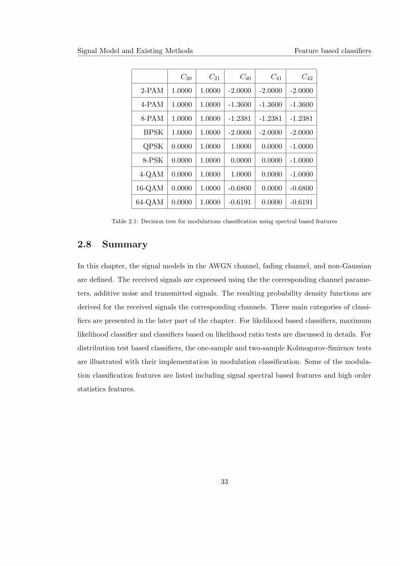
Signal Model and Existing Methods Feature based classifiers
C20 C21 C40 C41 C42
2-PAM 1.0000 1.0000 -2.0000 -2.0000 -2.0000
4-PAM 1.0000 1.0000 -1.3600 -1.3600 -1.3600
8-PAM 1.0000 1.0000 -1.2381 -1.2381 -1.2381
BPSK 1.0000 1.0000 -2.0000 -2.0000 -2.0000
QPSK 0.0000 1.0000 1.0000 0.0000 -1.0000
8-PSK 0.0000 1.0000 0.0000 0.0000 -1.0000
4-QAM 0.0000 1.0000 1.0000 0.0000 -1.0000
16-QAM 0.0000 1.0000 -0.6800 0.0000 -0.6800
64-QAM 0.0000 1.0000 -0.6191 0.0000 -0.6191
Table 2.1: Decision tree for modulations classification using spectral based features
2.8 Summary
In this chapter, the signal models in the AWGN channel, fading channel, and non-Gaussian
are defined. The received signals are expressed using the the corresponding channel parame-
ters, additive noise and transmitted signals. The resulting probability density functions are
derived for the received signals the corresponding channels. Three main categories of classi-
fiers are presented in the later part of the chapter. For likelihood based classifiers, maximum
likelihood classifier and classifiers based on likelihood ratio tests are discussed in details. For
distribution test based classifiers, the one-sample and two-sample Kolmogorov-Smirnov tests
are illustrated with their implementation in modulation classification. Some of the modula-
tion classification features are listed including signal spectral based features and high order
statistics features.
33

Chapter 3
Machine Learning for Modulation
Classification
3.1 Introduction
In Chapter 2, we list a collection of signal features for modulation classification. Some of the
classification decision making is based on multi-stage decision trees where each stage utilizes
a different feature. However, the need for designing the decision tree and optimization of
multiple decision thresholds is not very convenient. To overcome these problems, various
machine learning techniques have been employed to accomplish two major tasks in feature
based modulation classification. First, the machine learning techniques can provide a clas-
sification decision making process that is much easier to implement. Second, the machine
learning techniques can reduce the dimension of the feature set. It is achieved by feature
selection and feature generation, which enables the consideration of a more versatile feature
set while maintaining the computational efficiency of the classifier.
In this chapter, we first give two machine learning based classifiers namely k-nearest
neighbour classifier and support vector machine classifier for modulation classification in
combination with the features listed in Chapter 2. Next, the issue of feature space dimen-
sion reduction is explored through different algorithms including linear regression, genetic
34
Machine Learning for Modulation Classification Machine learning based classifiers
algorithm, and genetic programming.
3.2 Machine learning based classifiers
3.2.1 K-nearest neighbour classifier
The K-nearest Neighbour (KNN) classifier is a non-parametric algorithm which assigns the
class to a testing signal by analysing the number of nearest reference signals in the feature
space. It has been used to solve many different classification problems (Espejo et al., 2010;
Guo and Nandi, 2006).There are three mains steps in a KNN classifier.
To enable KNN classification, a reference feature space must be established first. The
features space should include M reference values of each feature from each modulation class.
The selection of M depends on the problem and is normally optimized heuristically. The
motivation for a larger number of M is that the reference feature space provides a more
accurate representation of the likely distribution of the testing signal features. On the other
hand, a larger M value is likely to impose a higher computational complexity in the later
steps of the KNN classifier.
For modulation classification, Zhu et al. suggested the use of training data from the same
signal source for the generation of reference feature values (Zhu et al., 2010). The advantage
of this approach is that the training signal shares the same source as the testing signal. Thus
the reference feature space is an accurate representation of the feature distribution of the
testing signal. Meanwhile, the construction of the reference feature space is really easy as
the only step required is to calculate the feature values for the training signals. However,
because of the random nature of the training signal, one cannot guarantee the accuracy of
the feature space to be high enough. Synthesised reference values are more controlled over
the construction of the reference feature space. Nevertheless, there need to be a hypothesised
feature distribution which is often not reliable.
Since the classifier requires the evaluation of distances between the test signal and refer-
ence signals, a distance metric must be defined before the search of neighbouring reference
signals can be achieved. There are many different metric systems that can be used for
35
Machine Learning for Modulation Classification Machine learning based classifiers
distance measurement in a KNN classifier. Euclidean distance is one of the most common
distance metrics for KNN classifier. Given a feature set F = {f1, f2...fL} with L number of
features, the Euclidean distance between feature set of signal A and B is calculated as
D(F(A),F(B)) =
√√√√ L∑l=1
[fl(A)− fl(B)]2 (3.1)
Having established the distance measurement, the classification decision is achieved by find-
ing the nearest number of reference samples and analysing the demography with these k
number of samples.
When the distances between test signal and all reference signals are evaluated, k number
of the reference signals are recorded as the k nearest neighbour. The selection of the value
of k should follow these rules:
• The value should ideally be a prime number, to avoid the case where the k neighbour
consisting of an equal number of reference signals from different classes.
• The value should be less than the total number of reference signals from a signal class.
• The value of k should be big enough to avoid false classification caused by outliers.
The actual optimization of the value k can be heuristic because it has been shown that the
classification does not vary much if the k value is in a reasonable range. The end classification
result is achieved by finding the majority of the k-nearest neighbour that share the same class.
This class will be assigned to the testing signal as the classification result. A pseudo code
for the KNN classifier implementation is given below.
The KNN is non-parametric and capable of multi-class classification. However it suffers
with increasing number of features which raises the dimension of the feature space and the
complexity of the distance calculation. Therefore, some sort of dimension reduction is needed
to make this method viable. Another disadvantage of the KNN classifier is that the features
contribution to the classification decision making is not weighted. There maybe cases where
the final distance is mostly affected by only one feature, if the distribution of this feature is
sparse and the distance between the testing sample and the reference sample on this feature
36
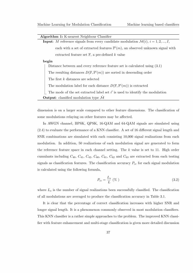
Machine Learning for Modulation Classification Machine learning based classifiers
Algorithm 1: K-nearest Neighbour Classifier
Input: M reference signals from every candidate modulation M(i), i = 1, 2, ..., I,
each with a set of extracted features Fi(m), an observed unknown signal with
extracted feature set F, a pre-defined k value
begin
Distance between and every reference feature set is calculated using (3.1)
The resulting distances D(F,Fi(m)) are sorted in descending order
The first k distances are selected
The modulation label for each distance D(F,Fi(m)) is extracted
The mode of the set extracted label set i′ is used to identify the modulation
Output: classified modulation type M
dimension is on a larger scale compared to other feature dimensions. The classification of
some modulations relaying on other features may be affected.
In AWGN channel, BPSK, QPSK, 16-QAM and 64-QAM signals are simulated using
(2.4) to evaluate the performance of a KNN classifier. A set of 16 different signal length and
SNR combinations are simulated with each consisting 10,000 signal realizations from each
modulation. In addition, 50 realizations of each modulation signal are generated to form
the reference feature space in each channel setting. The k value is set to 11. High order
cumulants including C40, C41, C42, C60, C61, C62 and C63 are extracted from each testing
signals as classification features. The classification accuracy Pcc for each signal modulation
is calculated using the following formula,
Pcc =LsL
(% ) (3.2)
where Ls is the number of signal realizations been successfully classified. The classification
of all modulations are averaged to produce the classification accuracy in Table 3.1.
It is clear that the percentage of correct classification increases with higher SNR and
longer signal length. It is a phenomenon commonly observed in most modulation classifiers.
This KNN classifier is a rather simple approaches to the problem. The improved KNN classi-
fier with feature enhancement and multi-stage classification is given more detailed discussion
37

Machine Learning for Modulation Classification Machine learning based classifiers
Number of Samples
SNR 512 1024 2048 4096
5 dB 79% 81% 91% 96%
10 dB 88% 93% 99% 100%
15 dB 90% 97% 100% 100%
20 dB 93% 98% 100% 100%
Table 3.1: Modulation classification performance of a KNN classifier in AWGN channels
in Section 3.3.3.
3.2.2 Support vector machine classifier
Support Vector Machine (SVM) provides another way to achieve classification in the existing
multi-dimensional feature space. It has been adopted for the classification of many differ-
ent data sets (Mustafa and Doroslovacki, 2004; Polat and Gune, 2007; Akay, 2009). SVM
achieve classification by finding the hyperplane that separates data from different classes.
The hyperplane, meanwhile, is optimized by maximizing its distance to the signal samples
on each side of the hyper-plane. Depending on the nature of the signal being classified, the
SVM classifiers can be divided into linear and non-linear versions.
The linear SVM classifiers have linear kernels. The kernel is defined by
K(x,w) = xTw (3.3)
where x = [x1...xK ] is the input feature vector and is the weight vector to be optimized.
The kernel defines a linear separation hyperplane (Theodoridis, 2008)
g(x) = xTw + w0 (3.4)
where w0 is a constant. The classification of a two-class (between modulation candidate
M(a) and M(b)) problem is achieved by simply using the sign of g(x)
M =
M(a), g(x) = xTw + w0 ≥ 0
M(b), g(x) = xTw + w0 < 0(3.5)
38
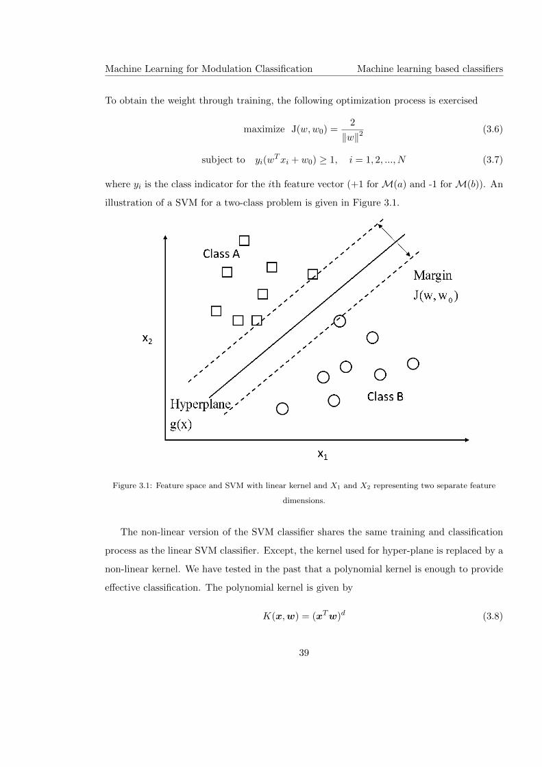
Machine Learning for Modulation Classification Machine learning based classifiers
To obtain the weight through training, the following optimization process is exercised
maximize J(w,w0) =2
‖w‖2(3.6)
subject to yi(wTxi + w0) ≥ 1, i = 1, 2, ..., N (3.7)
where yi is the class indicator for the ith feature vector (+1 forM(a) and -1 forM(b)). An
illustration of a SVM for a two-class problem is given in Figure 3.1.
Figure 3.1: Feature space and SVM with linear kernel and X1 and X2 representing two separate feature
dimensions.
The non-linear version of the SVM classifier shares the same training and classification
process as the linear SVM classifier. Except, the kernel used for hyper-plane is replaced by a
non-linear kernel. We have tested in the past that a polynomial kernel is enough to provide
effective classification. The polynomial kernel is given by
K(x,w) = (xTw)d (3.8)
39
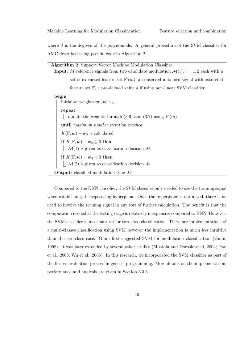
Machine Learning for Modulation Classification Feature selection and combination
where d is the degrees of the polynomials. A general procedure of the SVM classifier for
AMC described using pseudo code in Algorithm 2.
Algorithm 2: Support Vector Machine Modulation Classifier
Input: M reference signals from two candidate modulationM(i), i = 1, 2 each with a
set of extracted feature set Fi(m), an observed unknown signal with extracted
feature set F, a pre-defined value d if using non-linear SVM classifier
begin
initialize weights w and w0
repeat
update the weights through (3.6) and (3.7) using Fi(m)
until maximum number iteration reached
K(F,w) + w0 is calculated
if K(F,w) + w0 ≥ 0 then
M(1) is given as classification decision Mif K(F,w) + w0 < 0 then
M(2) is given as classification decision M
Output: classified modulation type M
Compared to the KNN classifier, the SVM classifier only needed to use the training signal
when establishing the separating hyperplane. Once the hyperplane is optimized, there is no
need to involve the training signal in any sort of further calculation. The benefit is that the
computation needed at the testing stage is relatively inexpensive compared to KNN. However,
the SVM classifier is most natural for two-class classification. There are implementations of
a multi-classes classification using SVM however the implementation is much less intuitive
than the two-class case. Gunn first suggested SVM for modulation classification (Gunn,
1998). It was later extended by several other studies (Mustafa and Doroslovacki, 2004; Dan
et al., 2005; Wu et al., 2005). In this research, we incorporated the SVM classifier as part of
the fitness evaluation process in genetic programming. More details on the implementation,
performance and analysis are given in Section 3.3.3.
40

Machine Learning for Modulation Classification Feature selection and combination
3.3 Feature selection and combination
For both KNN and SVM classifier, it is always preferable to have as many features as possible
for improving the classification accuracy. However, both classifiers suffer when the number
of features increase. That is why reducing the feature space dimension is necessary. Using
machine learning algorithms, there are two ways to do so. First, feature space dimension
can be reduced by eliminating some of the features which make less or no contribution to
the classification task. Second, feature space dimension can be reduced by combining the
existing feature into fewer new features.
3.3.1 Logistic regression
While feature selection is an effective way to reduce the complexity for a feature based mod-
ulation classifier, the elimination of a feature can sometimes be destructive. That is without
mentioning that sometime the features are all useful to some degree and the elimination
of any feature can be destructive for the classification performance. In this case, a more
conservative approach is needed for dimension reduction. That is why feature combination
has been considered for not just the reduction of feature dimension but also for enhancing
the performance of these features.
To begin with, linear combination of the features is the simplest but often effect way of
the combining the features. Assuming we are combining number of existing features into a
single new feature, the linear combination is given by
fnew = w0 +K∑k=1
wkfk (3.9)
where wk is the weight of the kth feature , w0 is a constant, and K is the total number of
features available for combination. The process to optimize these weights is called logistic
regression which aims to maximize the difference of the new feature value between different
classes. It has been adopted by Zhu et al. in the dimension reduction for distribution based
features (Zhu et al., 2013c).
There are two common logistic regression tools in the family of generalized linear regres-
sion algorithms namely binomial logistic regression and multinomial logistic regression. The
41
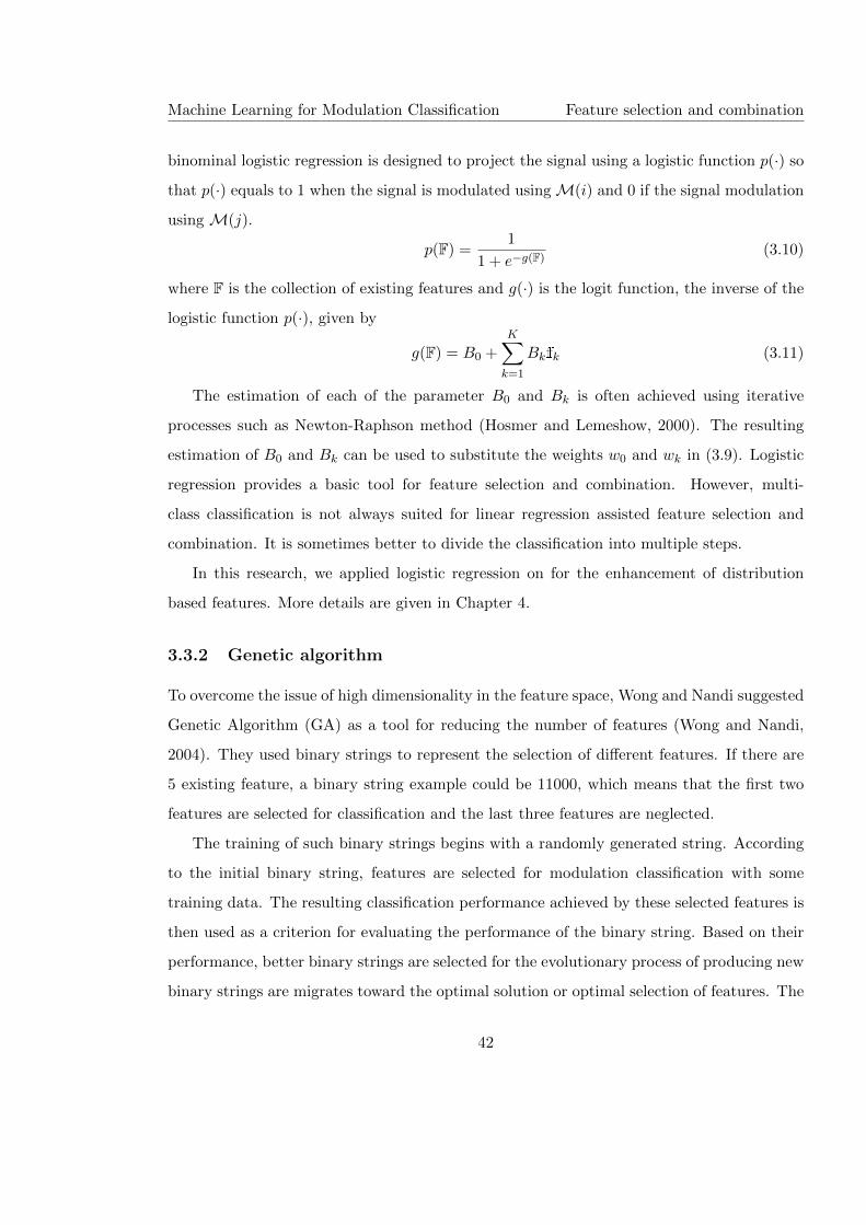
Machine Learning for Modulation Classification Feature selection and combination
binominal logistic regression is designed to project the signal using a logistic function p(·) so
that p(·) equals to 1 when the signal is modulated usingM(i) and 0 if the signal modulation
using M(j).
p(F) =1
1 + e−g(F)(3.10)
where F is the collection of existing features and g(·) is the logit function, the inverse of the
logistic function p(·), given by
g(F) = B0 +K∑k=1
Bkfk (3.11)
The estimation of each of the parameter B0 and Bk is often achieved using iterative
processes such as Newton-Raphson method (Hosmer and Lemeshow, 2000). The resulting
estimation of B0 and Bk can be used to substitute the weights w0 and wk in (3.9). Logistic
regression provides a basic tool for feature selection and combination. However, multi-
class classification is not always suited for linear regression assisted feature selection and
combination. It is sometimes better to divide the classification into multiple steps.
In this research, we applied logistic regression on for the enhancement of distribution
based features. More details are given in Chapter 4.
3.3.2 Genetic algorithm
To overcome the issue of high dimensionality in the feature space, Wong and Nandi suggested
Genetic Algorithm (GA) as a tool for reducing the number of features (Wong and Nandi,
2004). They used binary strings to represent the selection of different features. If there are
5 existing feature, a binary string example could be 11000, which means that the first two
features are selected for classification and the last three features are neglected.
The training of such binary strings begins with a randomly generated string. According
to the initial binary string, features are selected for modulation classification with some
training data. The resulting classification performance achieved by these selected features is
then used as a criterion for evaluating the performance of the binary string. Based on their
performance, better binary strings are selected for the evolutionary process of producing new
binary strings are migrates toward the optimal solution or optimal selection of features. The
42
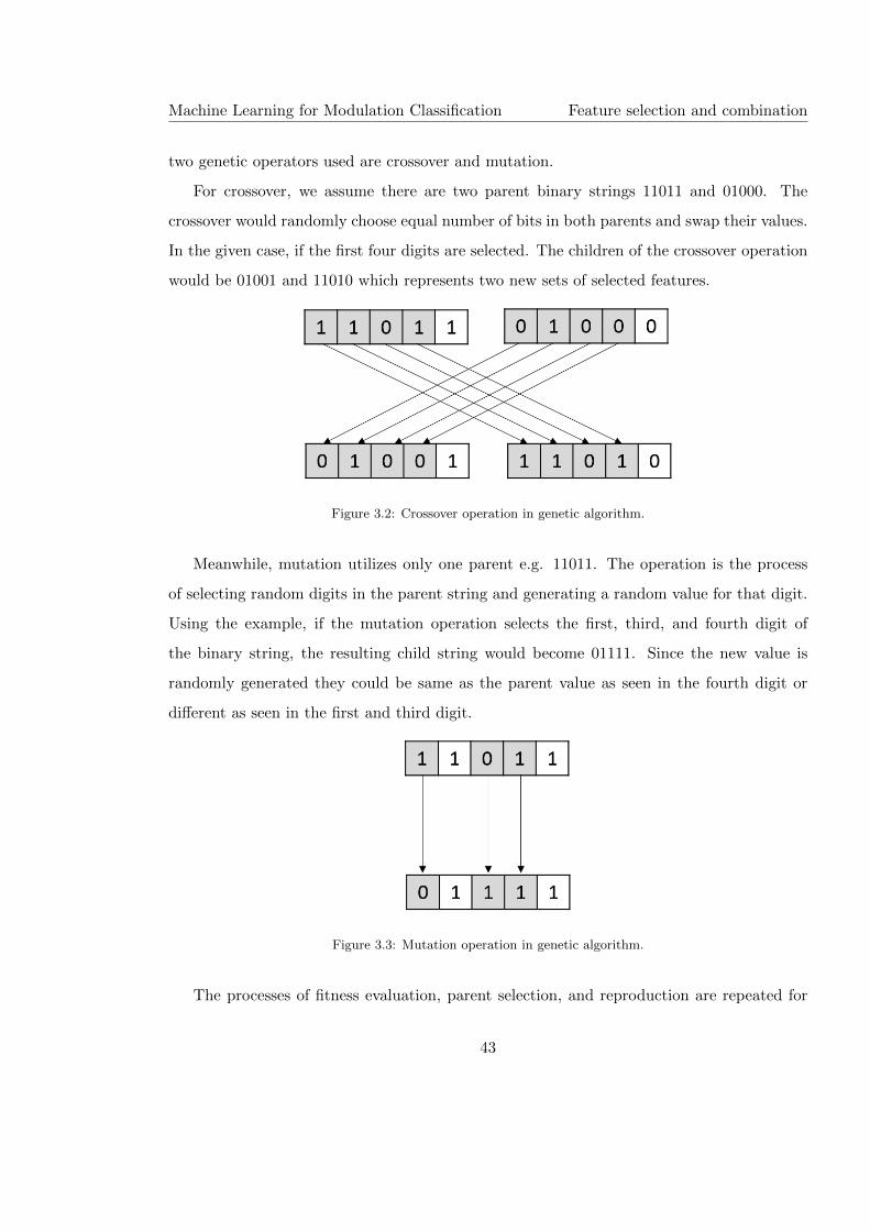
Machine Learning for Modulation Classification Feature selection and combination
two genetic operators used are crossover and mutation.
For crossover, we assume there are two parent binary strings 11011 and 01000. The
crossover would randomly choose equal number of bits in both parents and swap their values.
In the given case, if the first four digits are selected. The children of the crossover operation
would be 01001 and 11010 which represents two new sets of selected features.
Figure 3.2: Crossover operation in genetic algorithm.
Meanwhile, mutation utilizes only one parent e.g. 11011. The operation is the process
of selecting random digits in the parent string and generating a random value for that digit.
Using the example, if the mutation operation selects the first, third, and fourth digit of
the binary string, the resulting child string would become 01111. Since the new value is
randomly generated they could be same as the parent value as seen in the fourth digit or
different as seen in the first and third digit.
Figure 3.3: Mutation operation in genetic algorithm.
The processes of fitness evaluation, parent selection, and reproduction are repeated for
43
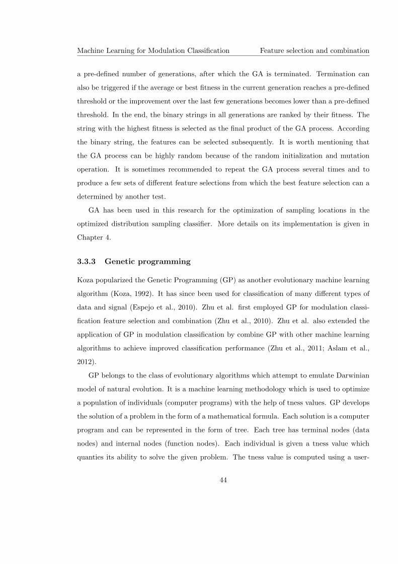
Machine Learning for Modulation Classification Feature selection and combination
a pre-defined number of generations, after which the GA is terminated. Termination can
also be triggered if the average or best fitness in the current generation reaches a pre-defined
threshold or the improvement over the last few generations becomes lower than a pre-defined
threshold. In the end, the binary strings in all generations are ranked by their fitness. The
string with the highest fitness is selected as the final product of the GA process. According
the binary string, the features can be selected subsequently. It is worth mentioning that
the GA process can be highly random because of the random initialization and mutation
operation. It is sometimes recommended to repeat the GA process several times and to
produce a few sets of different feature selections from which the best feature selection can a
determined by another test.
GA has been used in this research for the optimization of sampling locations in the
optimized distribution sampling classifier. More details on its implementation is given in
Chapter 4.
3.3.3 Genetic programming
Koza popularized the Genetic Programming (GP) as another evolutionary machine learning
algorithm (Koza, 1992). It has since been used for classification of many different types of
data and signal (Espejo et al., 2010). Zhu et al. first employed GP for modulation classi-
fication feature selection and combination (Zhu et al., 2010). Zhu et al. also extended the
application of GP in modulation classification by combine GP with other machine learning
algorithms to achieve improved classification performance (Zhu et al., 2011; Aslam et al.,
2012).
GP belongs to the class of evolutionary algorithms which attempt to emulate Darwinian
model of natural evolution. It is a machine learning methodology which is used to optimize
a population of individuals (computer programs) with the help of tness values. GP develops
the solution of a problem in the form of a mathematical formula. Each solution is a computer
program and can be represented in the form of tree. Each tree has terminal nodes (data
nodes) and internal nodes (function nodes). Each individual is given a tness value which
quanties its ability to solve the given problem. The tness value is computed using a user-
44
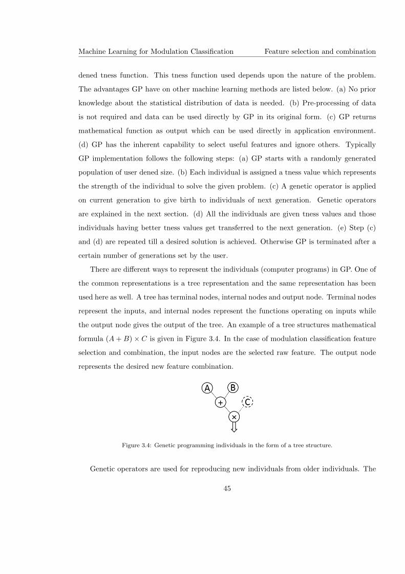
Machine Learning for Modulation Classification Feature selection and combination
dened tness function. This tness function used depends upon the nature of the problem.
The advantages GP have on other machine learning methods are listed below. (a) No prior
knowledge about the statistical distribution of data is needed. (b) Pre-processing of data
is not required and data can be used directly by GP in its original form. (c) GP returns
mathematical function as output which can be used directly in application environment.
(d) GP has the inherent capability to select useful features and ignore others. Typically
GP implementation follows the following steps: (a) GP starts with a randomly generated
population of user dened size. (b) Each individual is assigned a tness value which represents
the strength of the individual to solve the given problem. (c) A genetic operator is applied
on current generation to give birth to individuals of next generation. Genetic operators
are explained in the next section. (d) All the individuals are given tness values and those
individuals having better tness values get transferred to the next generation. (e) Step (c)
and (d) are repeated till a desired solution is achieved. Otherwise GP is terminated after a
certain number of generations set by the user.
There are different ways to represent the individuals (computer programs) in GP. One of
the common representations is a tree representation and the same representation has been
used here as well. A tree has terminal nodes, internal nodes and output node. Terminal nodes
represent the inputs, and internal nodes represent the functions operating on inputs while
the output node gives the output of the tree. An example of a tree structures mathematical
formula (A+B)× C is given in Figure 3.4. In the case of modulation classification feature
selection and combination, the input nodes are the selected raw feature. The output node
represents the desired new feature combination.
Figure 3.4: Genetic programming individuals in the form of a tree structure.
Genetic operators are used for reproducing new individuals from older individuals. The
45
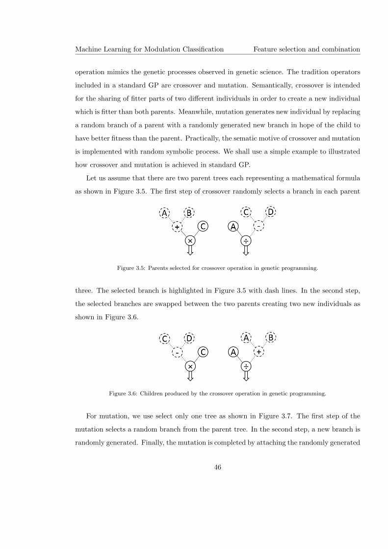
Machine Learning for Modulation Classification Feature selection and combination
operation mimics the genetic processes observed in genetic science. The tradition operators
included in a standard GP are crossover and mutation. Semantically, crossover is intended
for the sharing of fitter parts of two different individuals in order to create a new individual
which is fitter than both parents. Meanwhile, mutation generates new individual by replacing
a random branch of a parent with a randomly generated new branch in hope of the child to
have better fitness than the parent. Practically, the sematic motive of crossover and mutation
is implemented with random symbolic process. We shall use a simple example to illustrated
how crossover and mutation is achieved in standard GP.
Let us assume that there are two parent trees each representing a mathematical formula
as shown in Figure 3.5. The first step of crossover randomly selects a branch in each parent
Figure 3.5: Parents selected for crossover operation in genetic programming.
three. The selected branch is highlighted in Figure 3.5 with dash lines. In the second step,
the selected branches are swapped between the two parents creating two new individuals as
shown in Figure 3.6.
Figure 3.6: Children produced by the crossover operation in genetic programming.
For mutation, we use select only one tree as shown in Figure 3.7. The first step of the
mutation selects a random branch from the parent tree. In the second step, a new branch is
randomly generated. Finally, the mutation is completed by attaching the randomly generated
46
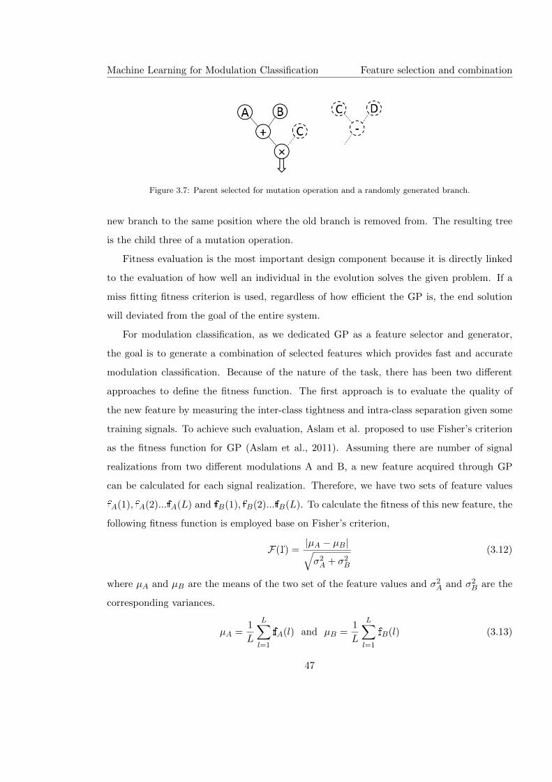
Machine Learning for Modulation Classification Feature selection and combination
Figure 3.7: Parent selected for mutation operation and a randomly generated branch.
new branch to the same position where the old branch is removed from. The resulting tree
is the child three of a mutation operation.
Fitness evaluation is the most important design component because it is directly linked
to the evaluation of how well an individual in the evolution solves the given problem. If a
miss fitting fitness criterion is used, regardless of how efficient the GP is, the end solution
will deviated from the goal of the entire system.
For modulation classification, as we dedicated GP as a feature selector and generator,
the goal is to generate a combination of selected features which provides fast and accurate
modulation classification. Because of the nature of the task, there has been two different
approaches to define the fitness function. The first approach is to evaluate the quality of
the new feature by measuring the inter-class tightness and intra-class separation given some
training signals. To achieve such evaluation, Aslam et al. proposed to use Fisher’s criterion
as the fitness function for GP (Aslam et al., 2011). Assuming there are number of signal
realizations from two different modulations A and B, a new feature acquired through GP
can be calculated for each signal realization. Therefore, we have two sets of feature values
fA(1), fA(2)...fA(L) and fB(1), fB(2)...fB(L). To calculate the fitness of this new feature, the
following fitness function is employed base on Fisher’s criterion,
F(f) =|µA − µB|√σ2A + σ2
B
(3.12)
where µA and µB are the means of the two set of the feature values and σ2A and σ2
B are the
corresponding variances.
µA =1
L
L∑l=1
fA(l) and µB =1
L
L∑l=1
fB(l) (3.13)
47

Machine Learning for Modulation Classification Feature selection and combination
σ2A =
1
L
L∑l=1
[fA(l)− µA]2 and σ2B =
1
L
L∑l=1
[fB(l)− µB]2 (3.14)
It is obvious that the nominator measures the separation of the features from different mod-
ulation signal and the denominator measure the tightness of the features from the same
modulation signals. Therefore, the fitness function matches the desired property of an effec-
tive feature for modulation classification. However, there are two drawbacks of the Fisher’s
criterion for fitness evaluation. First, the criterion is developed with the assumption of the
statistic being normally distributed. In the case of GP generated features, it is very difficult
to establish the distribution of a new feature because the features can be a very complicated
combination of many existing features. That is without mentioning the normality need to
be met for each new feature which various dramatically because of the random nature of
GP. The genetic operators constantly maintain the diversity in the populations resulting in
new features of diverse distributions. Secondly, in practice, there are cases where the trained
new feature may converge to have minimum amount of difference in their mean difference
while having very small variance. In other cases, the new feature can have very big mean
difference while the variance also being infinitely big.
Meanwhile, there is another approach which does not share the flaws of the Fisher’s
criterion based fitness evaluation. As the ultimate goal for the new feature is to enhance
the classification performance, we used a small set of training signals in the GP evaluation
and incorporated a computational efficient classifier in the fitness evaluation (Zhu et al.,
2010). The fitness, in this case, is evaluated by directly classifying the training signals with
a classifier from which the average classification accuracy is used as the fitness value.
In the first case, we employed the KNN classifier for the fitness evaluation. Different from
conventional fitness evaluation, the tree output from each individual is not directly utilized
for fitness calculation having employed the target value from the training input. Instead,
the output is used as a new feature for the KNN classifier with some of the training data
used as reference samples and the remaining training data used for evaluating trees. The
classification results from KNN classifier are obtained as described in earlier in this section.
Once the classification is finished, the result is returned to the fitness calculation function
48
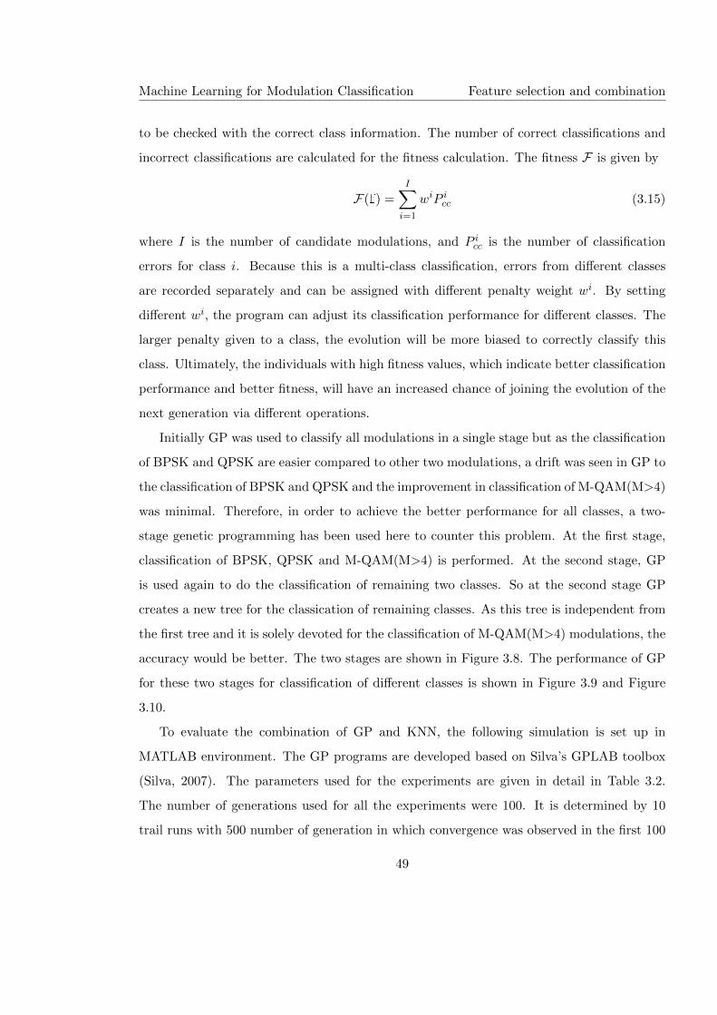
Machine Learning for Modulation Classification Feature selection and combination
to be checked with the correct class information. The number of correct classifications and
incorrect classifications are calculated for the fitness calculation. The fitness F is given by
F(f) =I∑i=1
wiP icc (3.15)
where I is the number of candidate modulations, and P icc is the number of classification
errors for class i. Because this is a multi-class classification, errors from different classes
are recorded separately and can be assigned with different penalty weight wi. By setting
different wi, the program can adjust its classification performance for different classes. The
larger penalty given to a class, the evolution will be more biased to correctly classify this
class. Ultimately, the individuals with high fitness values, which indicate better classification
performance and better fitness, will have an increased chance of joining the evolution of the
next generation via different operations.
Initially GP was used to classify all modulations in a single stage but as the classification
of BPSK and QPSK are easier compared to other two modulations, a drift was seen in GP to
the classification of BPSK and QPSK and the improvement in classification of M-QAM(M>4)
was minimal. Therefore, in order to achieve the better performance for all classes, a two-
stage genetic programming has been used here to counter this problem. At the first stage,
classification of BPSK, QPSK and M-QAM(M>4) is performed. At the second stage, GP
is used again to do the classification of remaining two classes. So at the second stage GP
creates a new tree for the classication of remaining classes. As this tree is independent from
the first tree and it is solely devoted for the classification of M-QAM(M>4) modulations, the
accuracy would be better. The two stages are shown in Figure 3.8. The performance of GP
for these two stages for classification of different classes is shown in Figure 3.9 and Figure
3.10.
To evaluate the combination of GP and KNN, the following simulation is set up in
MATLAB environment. The GP programs are developed based on Silva’s GPLAB toolbox
(Silva, 2007). The parameters used for the experiments are given in detail in Table 3.2.
The number of generations used for all the experiments were 100. It is determined by 10
trail runs with 500 number of generation in which convergence was observed in the first 100
49
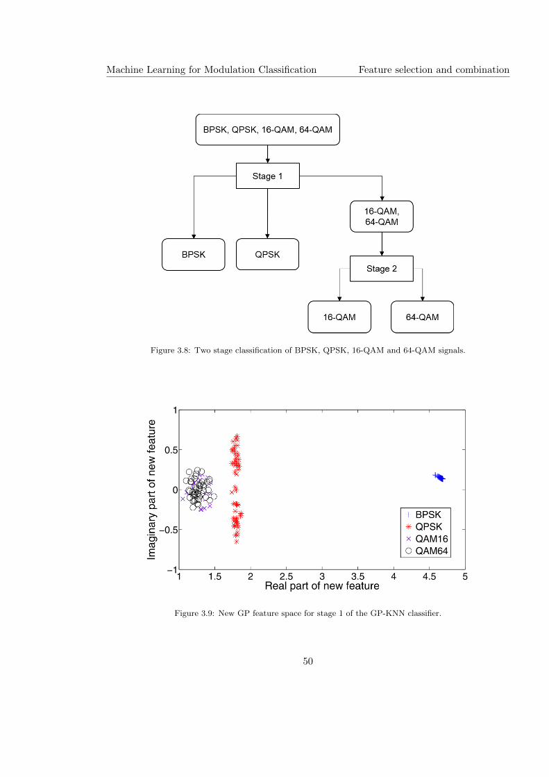
Machine Learning for Modulation Classification Feature selection and combination
Figure 3.8: Two stage classification of BPSK, QPSK, 16-QAM and 64-QAM signals.
Figure 3.9: New GP feature space for stage 1 of the GP-KNN classifier.
50

Machine Learning for Modulation Classification Feature selection and combination
Figure 3.10: New GP feature space for stage 2 of the GP-KNN classifier.
Parameters Values
Number of generations 100
Population size 25
Function pool plus, minus, times, reciprocal, negator, abs,
sqrt, sin, cos, tan, asin, acos, tanh, mylog
Terminal pool HOS features
Genetic operators crossover and mutation
Operator probabilities 90% and 10%
Tree generation ramped half-and-half
Initial maximum depth 28
Selection operator lexictour
Elitism replace
Table 3.2: Parameters used in genetic programming and KNN classifier.
51
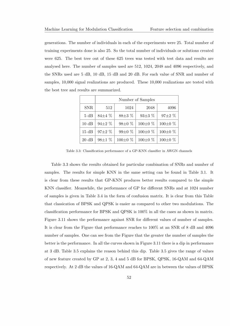
Machine Learning for Modulation Classification Feature selection and combination
generations. The number of individuals in each of the experiments were 25. Total number of
training experiments done is also 25. So the total number of individuals or solutions created
were 625. The best tree out of these 625 trees was tested with test data and results are
analysed here. The number of samples used are 512, 1024, 2048 and 4096 respectively, and
the SNRs used are 5 dB, 10 dB, 15 dB and 20 dB. For each value of SNR and number of
samples, 10,000 signal realizations are produced. These 10,000 realizations are tested with
the best tree and results are summarized.
Number of Samples
SNR 512 1024 2048 4096
5 dB 84±4 % 88±3 % 93±3 % 97±2 %
10 dB 94±2 % 98±0 % 100±0 % 100±0 %
15 dB 97±2 % 99±0 % 100±0 % 100±0 %
20 dB 98±1 % 100±0 % 100±0 % 100±0 %
Table 3.3: Classification performance of a GP-KNN classifier in AWGN channels
Table 3.3 shows the results obtained for particular combination of SNRs and number of
samples. The results for simple KNN in the same setting can be found in Table 3.1. It
is clear from these results that GP-KNN produces better results compared to the simple
KNN classifier. Meanwhile, the performance of GP for different SNRs and at 1024 number
of samples is given in Table 3.4 in the form of confusion matrix. It is clear from this Table
that classication of BPSK and QPSK is easier as compared to other two modulations. The
classification performance for BPSK and QPSK is 100% in all the cases as shown in matrix.
Figure 3.11 shows the performance against SNR for different values of number of samples.
It is clear from the Figure that performance reaches to 100% at an SNR of 8 dB and 4096
number of samples. One can see from the Figure that the greater the number of samples the
better is the performance. In all the curves shown in Figure 3.11 there is a dip in performance
at 3 dB. Table 3.5 explains the reason behind this dip. Table 3.5 gives the range of values
of new feature created by GP at 2, 3, 4 and 5 dB for BPSK, QPSK, 16-QAM and 64-QAM
respectively. At 2 dB the values of 16-QAM and 64-QAM are in between the values of BPSK
52
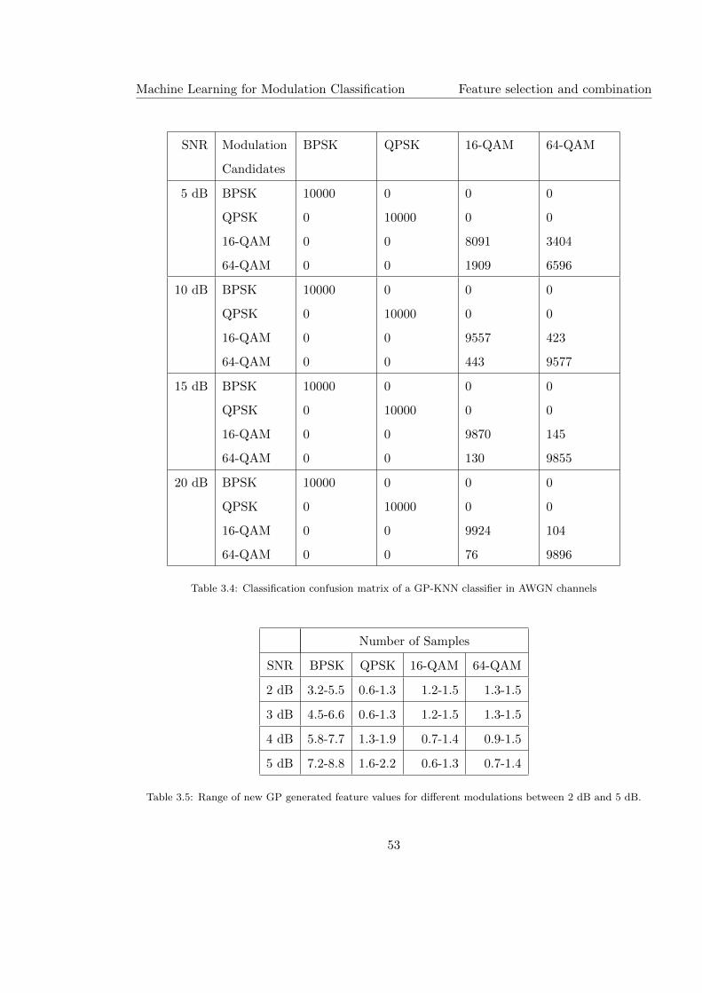
Machine Learning for Modulation Classification Feature selection and combination
SNR Modulation
Candidates
BPSK QPSK 16-QAM 64-QAM
5 dB BPSK
QPSK
16-QAM
64-QAM
10000
0
0
0
0
10000
0
0
0
0
8091
1909
0
0
3404
6596
10 dB BPSK
QPSK
16-QAM
64-QAM
10000
0
0
0
0
10000
0
0
0
0
9557
443
0
0
423
9577
15 dB BPSK
QPSK
16-QAM
64-QAM
10000
0
0
0
0
10000
0
0
0
0
9870
130
0
0
145
9855
20 dB BPSK
QPSK
16-QAM
64-QAM
10000
0
0
0
0
10000
0
0
0
0
9924
76
0
0
104
9896
Table 3.4: Classification confusion matrix of a GP-KNN classifier in AWGN channels
Number of Samples
SNR BPSK QPSK 16-QAM 64-QAM
2 dB 3.2-5.5 0.6-1.3 1.2-1.5 1.3-1.5
3 dB 4.5-6.6 0.6-1.3 1.2-1.5 1.3-1.5
4 dB 5.8-7.7 1.3-1.9 0.7-1.4 0.9-1.5
5 dB 7.2-8.8 1.6-2.2 0.6-1.3 0.7-1.4
Table 3.5: Range of new GP generated feature values for different modulations between 2 dB and 5 dB.
53
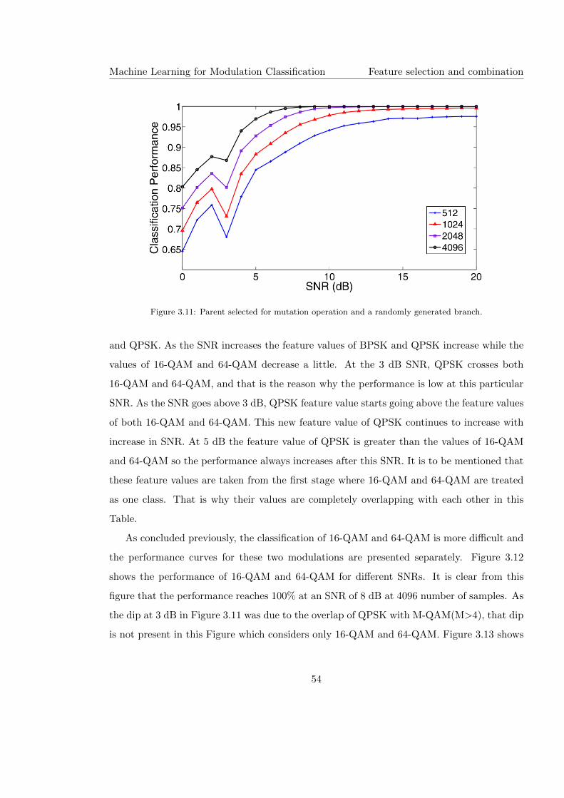
Machine Learning for Modulation Classification Feature selection and combination
Figure 3.11: Parent selected for mutation operation and a randomly generated branch.
and QPSK. As the SNR increases the feature values of BPSK and QPSK increase while the
values of 16-QAM and 64-QAM decrease a little. At the 3 dB SNR, QPSK crosses both
16-QAM and 64-QAM, and that is the reason why the performance is low at this particular
SNR. As the SNR goes above 3 dB, QPSK feature value starts going above the feature values
of both 16-QAM and 64-QAM. This new feature value of QPSK continues to increase with
increase in SNR. At 5 dB the feature value of QPSK is greater than the values of 16-QAM
and 64-QAM so the performance always increases after this SNR. It is to be mentioned that
these feature values are taken from the first stage where 16-QAM and 64-QAM are treated
as one class. That is why their values are completely overlapping with each other in this
Table.
As concluded previously, the classification of 16-QAM and 64-QAM is more difficult and
the performance curves for these two modulations are presented separately. Figure 3.12
shows the performance of 16-QAM and 64-QAM for different SNRs. It is clear from this
figure that the performance reaches 100% at an SNR of 8 dB at 4096 number of samples. As
the dip at 3 dB in Figure 3.11 was due to the overlap of QPSK with M-QAM(M>4), that dip
is not present in this Figure which considers only 16-QAM and 64-QAM. Figure 3.13 shows
54
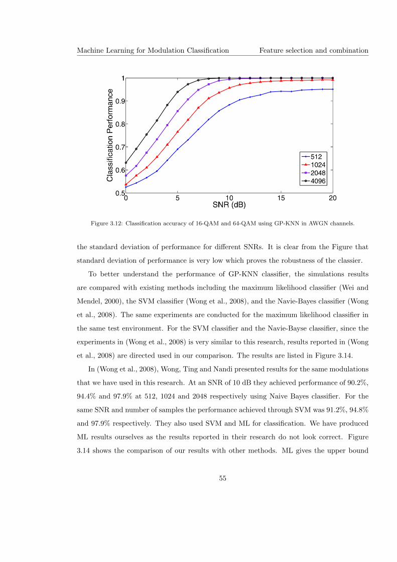
Machine Learning for Modulation Classification Feature selection and combination
Figure 3.12: Classification accuracy of 16-QAM and 64-QAM using GP-KNN in AWGN channels.
the standard deviation of performance for different SNRs. It is clear from the Figure that
standard deviation of performance is very low which proves the robustness of the classier.
To better understand the performance of GP-KNN classifier, the simulations results
are compared with existing methods including the maximum likelihood classifier (Wei and
Mendel, 2000), the SVM classifier (Wong et al., 2008), and the Navie-Bayes classifier (Wong
et al., 2008). The same experiments are conducted for the maximum likelihood classifier in
the same test environment. For the SVM classifier and the Navie-Bayse classifier, since the
experiments in (Wong et al., 2008) is very similar to this research, results reported in (Wong
et al., 2008) are directed used in our comparison. The results are listed in Figure 3.14.
In (Wong et al., 2008), Wong, Ting and Nandi presented results for the same modulations
that we have used in this research. At an SNR of 10 dB they achieved performance of 90.2%,
94.4% and 97.9% at 512, 1024 and 2048 respectively using Naive Bayes classifier. For the
same SNR and number of samples the performance achieved through SVM was 91.2%, 94.8%
and 97.9% respectively. They also used SVM and ML for classification. We have produced
ML results ourselves as the results reported in their research do not look correct. Figure
3.14 shows the comparison of our results with other methods. ML gives the upper bound
55

Machine Learning for Modulation Classification Feature selection and combination
Figure 3.13: Standard deviations of classification accuracy for 16-QAM and 64-QAM using GP-KNN in
AWGN channels.
Figure 3.14: Performance comparison of GP-KNN and other methods in AWGN channels.
56
Machine Learning for Modulation Classification Feature selection and combination
performance but have more computational complexity. It is clear from the figure that our
method gives better results compared to SVM and Naive Bayes method. Up to 4 dB SNR, the
performance of our method is same as the other two methods but after 4 dB, the performance
of our method improves compared to the other two. The maximum likelihood classifier (Wei
and Mendel, 2000), known to be optimum with perfect channel knowledge, is superior to all
other methods. However, its computational complexity also known to be high compared to
feature based classifiers.
Although many think that GP classifier will take a long time for classification as the
time for evolution could be very long. However, the computational complexity of the final
classifier is not to be confused with the training time of the classifier. Once we get the final
solution from training a GP, that final solution is used for classification and the computational
complexity of training a GP does not come into account while using the final solution.
The final solution produced by GP has inputs as cumulants and some functions from the
function pool. So the complexity of this particular solution really depends on the particular
cumulants and functions used by final GP solution. We have used sixth order cumulants and
the complexity of calculating these cumulants is lower than higher-order cumulants. The
function pool used has been presented in Table 3.2. Also the output used by this solution
is tested through KNN classifier which has complexity of O(nd) where n is the number of
reference samples and d represents dimensions of reference data. Here we have used two
dimensional data in the form of complex numbers but the function pool contains an abs
function which returns the magnitude of complex number as the output when the input is
a complex number. If the final solution is using the abs function in the last stage the final
output could be a real value. In a nutshell the complexity of our final classifier is O(nd)+
complexity of final solution.
3.4 Summary
In this chapter, we suggested different machine learning techniques for modulation classifi-
cation. The KNN classifier and SVM classifier are developed for feature based modulation
57
Machine Learning for Modulation Classification Feature selection and combination
classifier with supervised threshold optimization and decision making. Both classifiers can be
further enhanced using logistic regression, genetic algorithm, and genetic programming for
feature selection and combination. The simulation results show that the combination of GP
and KNN classifier is able to improve the classification accuracy of digital modulations over
existing classifier using the same features. While, the training stage is relatively complex,
the actual testing is much simpler and faster.
58
Chapter 4
Distribution Test Based Classifiers
4.1 Introduction
For the purpose of reducing the computational complexity, algorithms based on distribution
tests have been developed and presented in some recent publications. F. Wang and X.
Wang (Wang and Wang, 2010) used Kolmogorov-Smirnov test (Massey, 1951) to formulate a
solution by comparing the testing signal cumulative distribution functions with the reference
modulation’s CDFs. This method successfully achieved an improved performance especially
when limited signal length was available. It was pointed out in (Urriza et al., 2011) that
the K-S test approach requires the complete construction of signal CDFs which is relatively
complex and has the potential to be simplified. In the same paper, an optimized approach
was presented which reduced the complexity of KS classifier by analysing the CDFs between
two modulations at a single given location. When more than two modulations are considered,
multiple sets of sampling locations, each responsible for the classification of two modulations,
have been used. The classification accuracy is comparable to the KS classifier and the
complexity of the algorithm is reduced significantly. However, it is clear that the embedded
information in CDFs is underutilized and the robustness of this approach can be improved.
To overcome these limitations, we have developed the Optimized Distribution Sampling
Test (ODST) classifier which conducts simplified distribution tests at multiple optimized
sampling locations to achieve the balance between simplicity and performance. In addition,
59

Distribution Test Based Classifiers Optimized distribution sampling test
the signal distributions are extended to signal phase and magnitude where sampled statistics
are treated as features.
4.2 Optimized distribution sampling test
The classification procedure starts with the selection of the optimum sampling locations.
Once the optimum sampling locations are established, distribution parameters can be col-
lected at different locations and used for decision making. The exact procedure in each step
will be discussed in the following subsections. It is worth mentioning that we only considered
four modulation types namely: BPSK, QPSK, 16-QAM and 64-QAM. The multi-class clas-
sification problem is handled by dividing it into two 2-class classification steps. The actual
decision procedure is demonstrated in Figure 4.1. As the proposed method exploits the dif-
ferent CDFs between different M-QAM signal modulations and it is the nature of M-QAM
signals to exhibit different distribution on their real and imaginary components, the extension
of the proposed method for other M-QAM modulations can be easily implemented follow-
ing the sampling location optimization principle explained in Section 4.2.2 and the decision
value calculation explained in Section 4.2.3. However, with different modulation candidates,
the performance may vary depending on the specific M-QAM modulation being considered.
Lower level M-QAM modulations are normally easier to classify. Modulations with similar
constellation shape and similar number of symbols are more difficult to distinguish.
4.2.1 Phase offset compensation
In a fading channel, phase and frequency offsets are added along with some attenuation and
additive noise. The received signal after matched filtering and sampling is given by
r(n) = αej(2πfon+θo)s(n) + ω(n) (4.1)
where the residual intersymbol interference is omitted and treated as noise. We first consider
the phase offset. It is assumed here that fading is slow, thus the phase offset is consistent
for all signal samples. Instead of constructing a signal model with phase offset in mind,
60

Distribution Test Based Classifiers Optimized distribution sampling test
4-QAM, 16-QAM OR 64-QAM
D416D464
4-QAM 16-QAM OR 64-QAM
D1664
16-QAM 64-QAM
Figure 4.1: Two stage classification strategy in the ODST classifier.
it is easier to recover the received data from the transmitted form. As the rotation of the
constellation mapping would cause a significant amount of mismatching with the established
reference signal model, the Extended Maximum Likelihood (EML) estimator in (Zarzoso
and Nandi, 1999) is used for pre-processing the signal to recover the phase offset. The phase
estimation starts with the calculation of fourth-order complex statistics.
ξ =1
N
N∑n=1
ρ4nej4φn =
1
N
N∑n=1
(R{r(n)}+ jI{r(n)})4 (4.2)
ρn and φn come from the polar expression of the nth signal sample r(n) = ρnejφn among the
total number of N signal samples. The source kurtosis sum γ is also needed in the phase
estimation.
γ =1
N
N∑n=1
ρ4n − 8 =
1
N
N∑n=1
(R{r2(n)}+ I{r2(n)})2 − 8 (4.3)
61

Distribution Test Based Classifiers Optimized distribution sampling test
The phase offset θEML is then estimated using the fourth-order complex statistics and source
kurtosis sum calculated previously.
θEML =1
4angle(ξ · sign(γ)) (4.4)
Once the phase offset is estimated, it can be easily recovered by conducting the following
procedure
r(n) = r(n)/ejθEML (4.5)
and the PDF could be treated in the same way as in AWGN channel
fi(x) =1
σ√
2πe−
(x−Ai)2
2σ2 (4.6)
Frequency offset is added to the signal separately from the phase offset. Any frequency offset
is treated as noise in the investigation.
4.2.2 Sampling location optimization
In Kolmogorov-Smirnov Test, the similarity of two distributions is tested by finding the
maximum distance between the two distributions. However, it is limited by the fact that
outliers and other irregularities in the test signal distribution can cause the maximum dis-
tance to occur at a location which does not exhibit the best characteristic difference between
them. The effect becomes more significant when the signal length is reduced or the amount
of noise added is increased. Ultimately, the classification accuracy from different tests could
vary dramatically. To overcome this limitation, the ODST uses multiple sampling locations
estimated with theoretical analysis to achieve a more robust performance.
As the later distribution test will be based on CDFs from different signal modulations,
the main purpose of the sampling location optimization is to find locations where the two
CDFs from different modulations exhibit the biggest difference. In this research, we propose
to use the local optima on the CDFs’ differences as sampling locations.
There are two parameters to consider when searching for sampling locations: the number
of sampling points and their locations. Though more information from the distribution could
always help to improve the understanding of the signal, some contribute significantly more
62
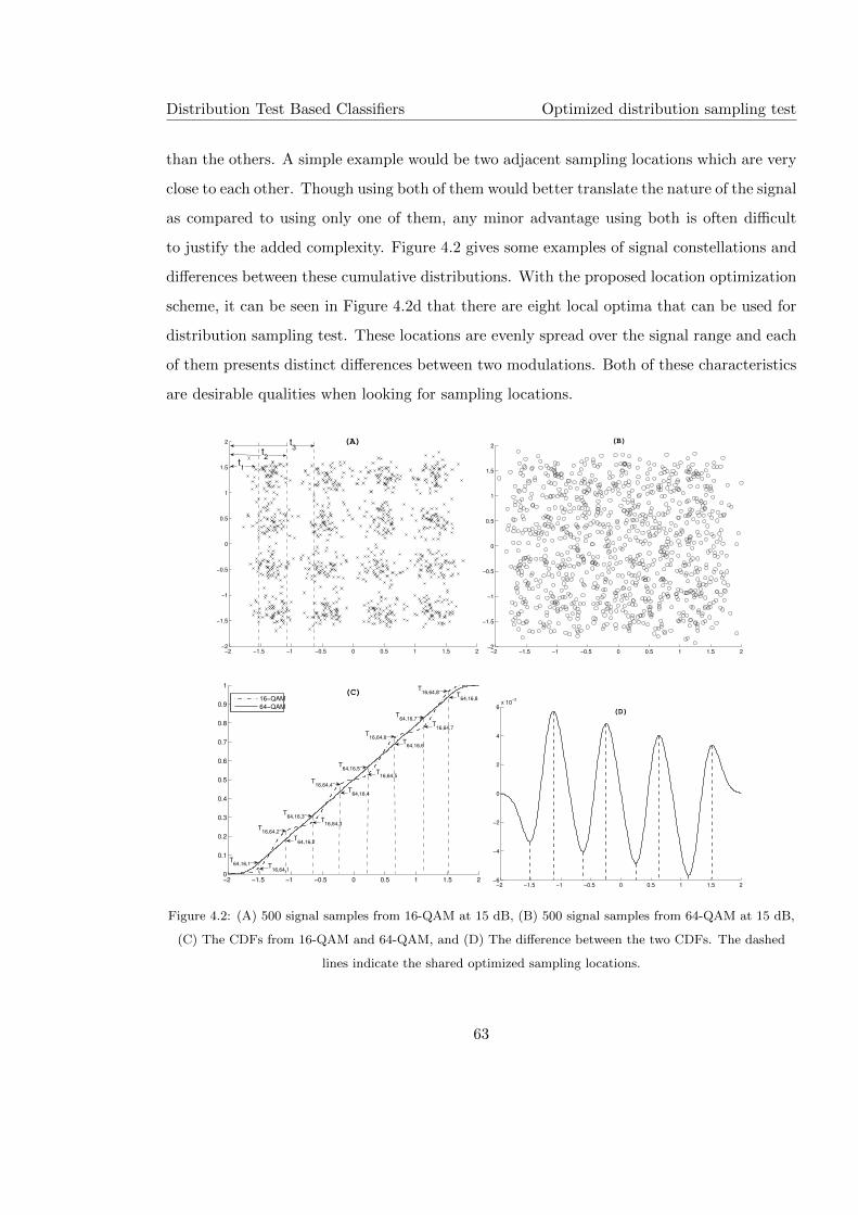
Distribution Test Based Classifiers Optimized distribution sampling test
than the others. A simple example would be two adjacent sampling locations which are very
close to each other. Though using both of them would better translate the nature of the signal
as compared to using only one of them, any minor advantage using both is often difficult
to justify the added complexity. Figure 4.2 gives some examples of signal constellations and
differences between these cumulative distributions. With the proposed location optimization
scheme, it can be seen in Figure 4.2d that there are eight local optima that can be used for
distribution sampling test. These locations are evenly spread over the signal range and each
of them presents distinct differences between two modulations. Both of these characteristics
are desirable qualities when looking for sampling locations.
−2 −1.5 −1 −0.5 0 0.5 1 1.5 2−2
−1.5
−1
−0.5
0
0.5
1
1.5
2 (A)
t2
t3
t1
−2 −1.5 −1 −0.5 0 0.5 1 1.5 2−2
−1.5
−1
−0.5
0
0.5
1
1.5
2(B)
−2 −1.5 −1 −0.5 0 0.5 1 1.5 20
0.1
0.2
0.3
0.4
0.5
0.6
0.7
0.8
0.9
1(C)
16−QAM
64−QAM
T64,16,1
T64,16,3
T16,64,5
T64,16,6
T16,64,8
T64,16,8
T16,64,2
T64,16,2
T16,64,1
T64,16,4
T16,64,3
T16,64,4
T64,16,5
T16,64,6
T16,64,7
T64,16,7
−2 −1.5 −1 −0.5 0 0.5 1 1.5 2−6
−4
−2
0
2
4
6x 10
−3
(D)
Figure 4.2: (A) 500 signal samples from 16-QAM at 15 dB, (B) 500 signal samples from 64-QAM at 15 dB,
(C) The CDFs from 16-QAM and 64-QAM, and (D) The difference between the two CDFs. The dashed
lines indicate the shared optimized sampling locations.
63
Distribution Test Based Classifiers Optimized distribution sampling test
We define l as a collection of sampling locations with lk being the individual points.
l = {lk, for k = 1, ..,K} (4.7)
Through extended observations of various type of signals and their distributions, we define
the optimum sampling locations to occur when the difference between CDFs from two classes
is locally optimum, for modulation A-QAM and B-QAM, this can be easily transformed into
the calculation of first derivative of their CDFs’ (FA and FB) difference
d
dx(FA(l)− FB(l)) = 0 (4.8)
The derivative of CDFs’ difference can also be replaced by probability distribution for both
modulations (fA and fB)
fA(l)− fB(l) =
IA∑i=1
(fAi(l))−IB∑i=1
(fBi(l)) = 0 (4.9)
where the PDF for each signal centroids (fAi and fBi) are defined previously in (2.6). IA and
IB correspond to the total number of centroids for each modulation on one signal dimension.
After the optimization of the sampling locations, the theoretical CDF values at sampling
locations for different modulations are collected for classification task as the reference data.
The reference data for A-QAM while considering the classification between A-QAM and
B-QAM is given as
TA,B = [TA,B,1, ..., TA,B,k] (4.10)
where
TA,B,k = FA(lk) (4.11)
FA is the CDF of modulation A-QAM. These values will be stored for later distribution tests.
Once the sampling locations are established, the distribution sampling could be converted
to simple counting tasks. The counted distribution parameter tk can be written as
tk =1
2N[N∑n=1
I(rX(n) < lk) +N∑n=1
I(rY (n) < lk)] (4.12)
where I(·) is an conditional function which returns 1 if the input is true and 0 if input is
false. The counting tasks at different locations are also illustrated in Figure 4.2a.
64

Distribution Test Based Classifiers Optimized distribution sampling test
4.2.3 Test statistics and decision making
The counting results are put into the classification context by finding the difference ∆t
between the counted value and the theoretical value from candidate modulations.
∆tA,B,k = |tk − TA,B,k| (4.13)
where ∆tA,B,k give the difference between testing signal distribution parameter and reference
value TA,B,k from candidate A. Likewise the difference between testing signal and candidate
B can be found as
∆tB,A,k = |tk − TB,A,k| (4.14)
In the standard uniformly weighted distance metric, the decision is made using all sampled
results with the same weight. The decision values for different 2-class classification situations
are defined as
DA,B =
K∑k=1
∆tA,B,k −K∑k=1
∆tB,A,k (4.15)
where DA,B compares the distance between testing signal and candidate A and the distance
between testing signal and candidate B. If DA,B ≥ 0, it means the tested signal is close to
candidate A and thus have a higher probability of being classified as candidate A. However
as there are more than two candidate modulations involved. The final decision can be made
according to a set of decision values.
M =
4QAM, D4,16 ≤ 0 & D4,64 < 0
16QAM, D4,16 > 0 & D16,64 ≤ 0
64QAM, D4,64 ≥ 0 & D16,64 > 0
(4.16)
The resulting M gives the estimated M value for the tested M-QAM signals. D4,16, D4,64
and D16,64 are decision values gathered from the previous stage.
Given the distance definition in (4.15), it is worth questioning the actual contribution of
each sampling locations. Though the optimization process attempts to find the best locations
with maximum amount of separation while conveying the full characteristic of the CDFs,
it is still possible for the local optima to be inefficient. For example, two local optimums
65
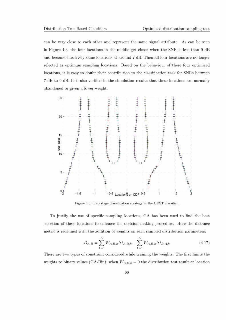
Distribution Test Based Classifiers Optimized distribution sampling test
can be very close to each other and represent the same signal attribute. As can be seen
in Figure 4.3, the four locations in the middle get closer when the SNR is less than 9 dB
and become effectively same locations at around 7 dB. Then all four locations are no longer
selected as optimum sampling locations. Based on the behaviour of these four optimized
locations, it is easy to doubt their contribution to the classification task for SNRs between
7 dB to 9 dB. It is also verified in the simulation results that these locations are normally
abandoned or given a lower weight.
−2 −1.5 −1 −0.5 0 0.5 1 1.5 20
5
10
15
20
25
Locations on CDF
SN
R (
dB
)
Figure 4.3: Two stage classification strategy in the ODST classifier.
To justify the use of specific sampling locations, GA has been used to find the best
selection of these locations to enhance the decision making procedure. Here the distance
metric is redefined with the addition of weights on each sampled distribution parameters.
DA,B =K∑k=1
WA,B,k∆tA,B,k −K∑k=1
WA,B,k∆tB,A,k (4.17)
There are two types of constraint considered while training the weights. The first limits the
weights to binary values (GA-Bin), when WA,B,k = 0 the distribution test result at location
66
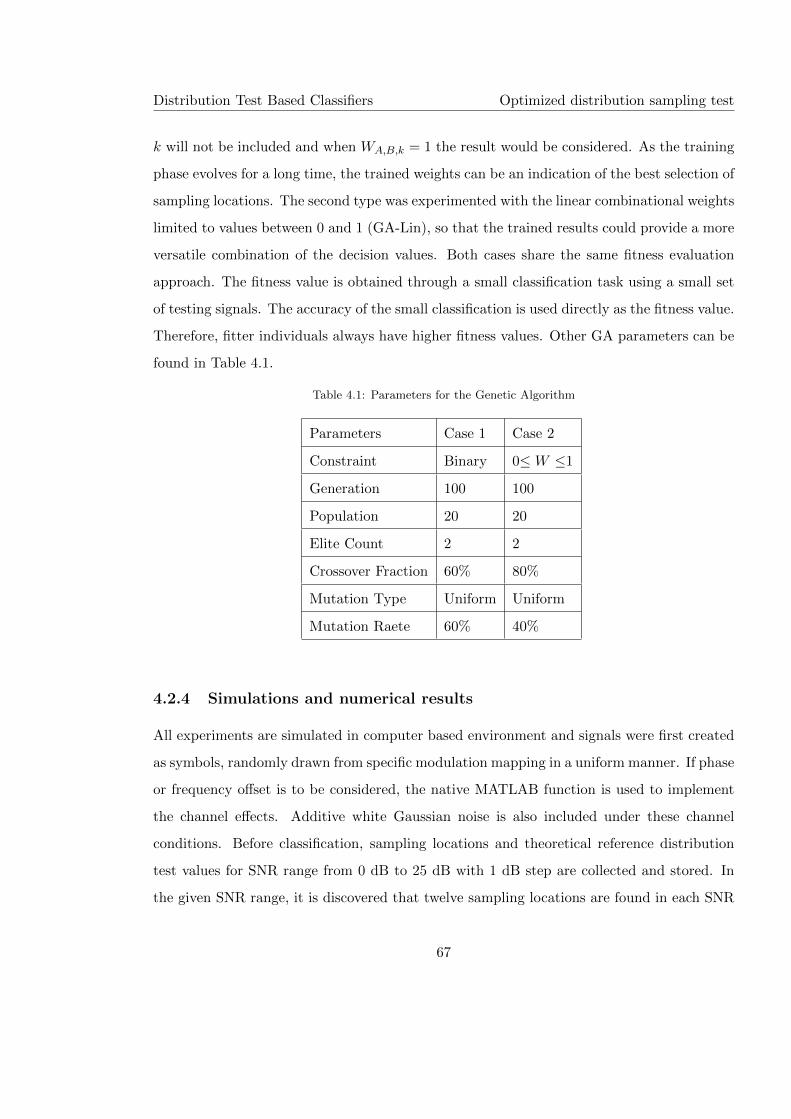
Distribution Test Based Classifiers Optimized distribution sampling test
k will not be included and when WA,B,k = 1 the result would be considered. As the training
phase evolves for a long time, the trained weights can be an indication of the best selection of
sampling locations. The second type was experimented with the linear combinational weights
limited to values between 0 and 1 (GA-Lin), so that the trained results could provide a more
versatile combination of the decision values. Both cases share the same fitness evaluation
approach. The fitness value is obtained through a small classification task using a small set
of testing signals. The accuracy of the small classification is used directly as the fitness value.
Therefore, fitter individuals always have higher fitness values. Other GA parameters can be
found in Table 4.1.
Table 4.1: Parameters for the Genetic Algorithm
Parameters Case 1 Case 2
Constraint Binary 0≤W ≤1
Generation 100 100
Population 20 20
Elite Count 2 2
Crossover Fraction 60% 80%
Mutation Type Uniform Uniform
Mutation Raete 60% 40%
4.2.4 Simulations and numerical results
All experiments are simulated in computer based environment and signals were first created
as symbols, randomly drawn from specific modulation mapping in a uniform manner. If phase
or frequency offset is to be considered, the native MATLAB function is used to implement
the channel effects. Additive white Gaussian noise is also included under these channel
conditions. Before classification, sampling locations and theoretical reference distribution
test values for SNR range from 0 dB to 25 dB with 1 dB step are collected and stored. In
the given SNR range, it is discovered that twelve sampling locations are found in each SNR
67
Distribution Test Based Classifiers Optimized distribution sampling test
scenario between 0 dB and 7 dB, and sixteen sampling locations are found when SNR is
between 8 dB and 25 dB. As two reference CDF values are needed at each sampling location
to complete the decision value calculation, there are a total number of 768 reference values
prepared for each given signal length.
During GA optimization, the fitness function is defined in the same way as in classifi-
cation problems where the classification accuracy is used as the fitness value. To reduce
the complexity of the training stage, only 1000 realizations from each modulation with a
signal length of N = 512 samples are used in the fitness evaluation process. The training
is repeated five times for each SNR value ranging from 0 dB to 10 dB. All signal data is
generated randomly at every fitness evaluation, which avoids weights being over-trained for a
specific set of signal data. In addition, with the two elites always being passed on to the next
generation, the possibly best solutions are always protected to some degree. The training
was repeated for five runs under each signal condition. The collections of weights which give
the best performance were selected for performance assessment with larger statistics at a
later stage.
When testing the performance of the proposed solution, maximum likelihood classifier,
the KS test, culumant based Genetic programming and k-nearest neighbour classifiers were
used for benchmarking purpose.
For the performance test in AWGN channel, two sets of experiments were conducted.
The first set of experiments focused on the classification accuracy under different noise levels.
Here, the signal length is fixed at 512 samples with the SNR ranging from 0 dB to 25 dB. Then
classifications of 100,000 signal realizations from each modulation were tested using ML, KS
test, GP-KNN and the proposed ODST classifier. The successful classification percentage
was calculated based on the number of successful classifications and the total number of
signal realizations. The results are presented in Figure 4.4. In the second set of experiments,
we tried to understand how the signal length influences the classification performance. In
this case, similar settings were used, except for SNR being fixed at 10 dB and sample size to
vary from 100 to 1000. The results are presented in Figure 4.5.
The classification performance under different amount of additive noise has always been
68

Distribution Test Based Classifiers Optimized distribution sampling test
0 2 4 6 8 10 12 14 16 18 2050
60
70
80
90
100
SNR (dB)
Cla
ssifi
cati
onA
ccura
cy(%
)
ODSTKS-Test
Cumulant-GPKNNML
Figure 4.4: Classification accuracy of 4-QAM, 16-QAM and 64-QAM using ODST in AWGN channel.
69

Distribution Test Based Classifiers Optimized distribution sampling test
200 400 600 800 1,00070
75
80
85
90
95
100
Signal Length
Cla
ssifi
cati
onA
ccura
cy(%
)
ODSTKS-Test
Cumulants-GPKNNML
Figure 4.5: Classification accuracy of 4-QAM, 16-QAM and 64-QAM using ODST in AWGN channel with
different signal length.
70
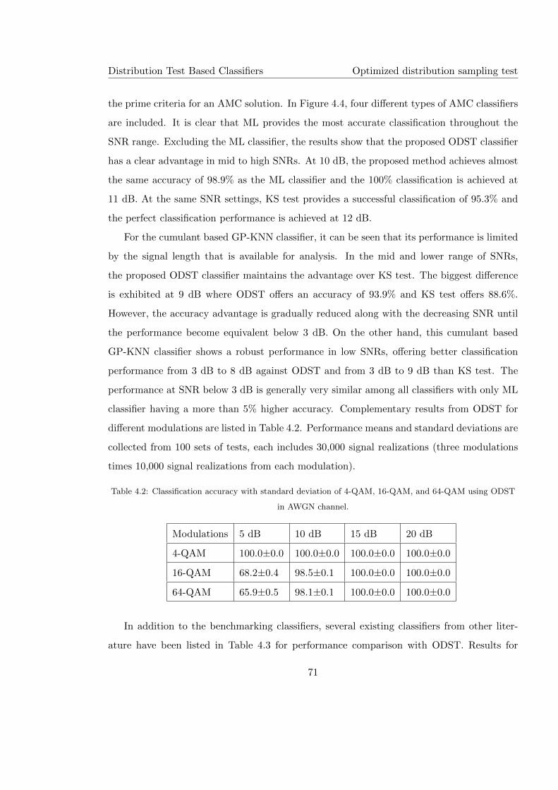
Distribution Test Based Classifiers Optimized distribution sampling test
the prime criteria for an AMC solution. In Figure 4.4, four different types of AMC classifiers
are included. It is clear that ML provides the most accurate classification throughout the
SNR range. Excluding the ML classifier, the results show that the proposed ODST classifier
has a clear advantage in mid to high SNRs. At 10 dB, the proposed method achieves almost
the same accuracy of 98.9% as the ML classifier and the 100% classification is achieved at
11 dB. At the same SNR settings, KS test provides a successful classification of 95.3% and
the perfect classification performance is achieved at 12 dB.
For the cumulant based GP-KNN classifier, it can be seen that its performance is limited
by the signal length that is available for analysis. In the mid and lower range of SNRs,
the proposed ODST classifier maintains the advantage over KS test. The biggest difference
is exhibited at 9 dB where ODST offers an accuracy of 93.9% and KS test offers 88.6%.
However, the accuracy advantage is gradually reduced along with the decreasing SNR until
the performance become equivalent below 3 dB. On the other hand, this cumulant based
GP-KNN classifier shows a robust performance in low SNRs, offering better classification
performance from 3 dB to 8 dB against ODST and from 3 dB to 9 dB than KS test. The
performance at SNR below 3 dB is generally very similar among all classifiers with only ML
classifier having a more than 5% higher accuracy. Complementary results from ODST for
different modulations are listed in Table 4.2. Performance means and standard deviations are
collected from 100 sets of tests, each includes 30,000 signal realizations (three modulations
times 10,000 signal realizations from each modulation).
Table 4.2: Classification accuracy with standard deviation of 4-QAM, 16-QAM, and 64-QAM using ODST
in AWGN channel.
Modulations 5 dB 10 dB 15 dB 20 dB
4-QAM 100.0±0.0 100.0±0.0 100.0±0.0 100.0±0.0
16-QAM 68.2±0.4 98.5±0.1 100.0±0.0 100.0±0.0
64-QAM 65.9±0.5 98.1±0.1 100.0±0.0 100.0±0.0
In addition to the benchmarking classifiers, several existing classifiers from other liter-
ature have been listed in Table 4.3 for performance comparison with ODST. Results for
71
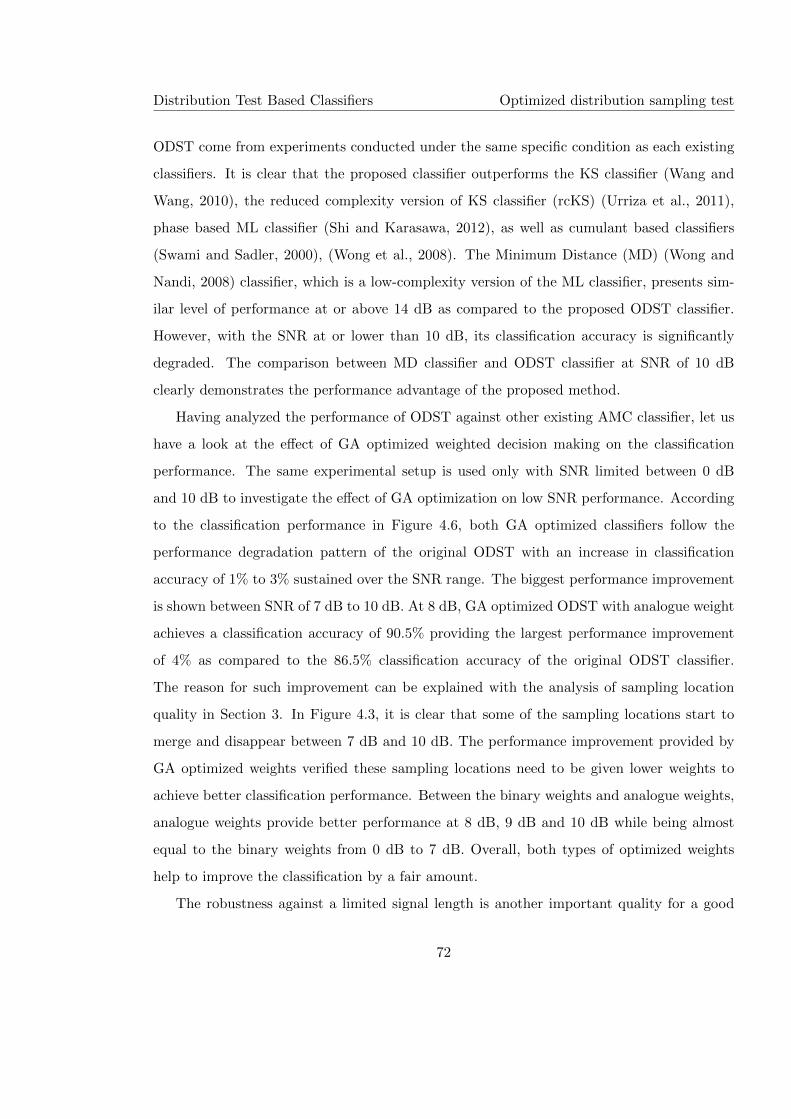
Distribution Test Based Classifiers Optimized distribution sampling test
ODST come from experiments conducted under the same specific condition as each existing
classifiers. It is clear that the proposed classifier outperforms the KS classifier (Wang and
Wang, 2010), the reduced complexity version of KS classifier (rcKS) (Urriza et al., 2011),
phase based ML classifier (Shi and Karasawa, 2012), as well as cumulant based classifiers
(Swami and Sadler, 2000), (Wong et al., 2008). The Minimum Distance (MD) (Wong and
Nandi, 2008) classifier, which is a low-complexity version of the ML classifier, presents sim-
ilar level of performance at or above 14 dB as compared to the proposed ODST classifier.
However, with the SNR at or lower than 10 dB, its classification accuracy is significantly
degraded. The comparison between MD classifier and ODST classifier at SNR of 10 dB
clearly demonstrates the performance advantage of the proposed method.
Having analyzed the performance of ODST against other existing AMC classifier, let us
have a look at the effect of GA optimized weighted decision making on the classification
performance. The same experimental setup is used only with SNR limited between 0 dB
and 10 dB to investigate the effect of GA optimization on low SNR performance. According
to the classification performance in Figure 4.6, both GA optimized classifiers follow the
performance degradation pattern of the original ODST with an increase in classification
accuracy of 1% to 3% sustained over the SNR range. The biggest performance improvement
is shown between SNR of 7 dB to 10 dB. At 8 dB, GA optimized ODST with analogue weight
achieves a classification accuracy of 90.5% providing the largest performance improvement
of 4% as compared to the 86.5% classification accuracy of the original ODST classifier.
The reason for such improvement can be explained with the analysis of sampling location
quality in Section 3. In Figure 4.3, it is clear that some of the sampling locations start to
merge and disappear between 7 dB and 10 dB. The performance improvement provided by
GA optimized weights verified these sampling locations need to be given lower weights to
achieve better classification performance. Between the binary weights and analogue weights,
analogue weights provide better performance at 8 dB, 9 dB and 10 dB while being almost
equal to the binary weights from 0 dB to 7 dB. Overall, both types of optimized weights
help to improve the classification by a fair amount.
The robustness against a limited signal length is another important quality for a good
72
Distribution Test Based Classifiers Optimized distribution sampling test
Table 4.3: Performance comparison between ODST and existing methods.
Classifier Modulation Channel Setting Accuracy ODST
KS 2-D 4-QAM
16-QAM
64-QAM
AWGN N = 100
10 dB
78.0% 85.2%
KS magnitude 4-QAM
16-QAM
64-QAM
AWGN N = 100
14 dB
87.0% 99.6%
rcKS 4-QAM
16-QAM
64-QAM
AWGN N = 50
10 dB
72.5% 77.3%
Phase Based ML 4-QAM, AWGN N = 1000
0 dB
73.5% 82.3%
16-QAM
MD 4-QAM, AWGN N = 100
10 dB
50.0% 86.5%
16-QAM
MD 4-QAM, AWGN N = 100
14 dB
91.5% 97.3%
16-QAM
Cumulants 16-QAM, Noise Free N = 10, 512 90.0% 100.0%
64-QAM
Cumulants Naive
Bayes
4-QAM
16-QAM
64-QAM
AWGN N = 512
10 dB
87.3% 98.5%
73

Distribution Test Based Classifiers Optimized distribution sampling test
0 2 4 6 8 10
60
70
80
90
100
SNR (dB)
Cla
ssifi
cati
onA
ccu
racy
(%)
ODSTGA-BinGA-Lin
Figure 4.6: Classification accuracy of 4-QAM, 16-QAM and 64-QAM using GA and ODST in AWGN
channel.
AMC classification. In the experiments, same four classifiers are tested and compared in
Figure 4.5. Again, ML excels in all signal length from N = 100 to N = 1000. Excluding
ML classifier, ODST is the best among the remaining classifiers. The largest performance
difference of ODST against ML is about 5% at N = 100. As the signal length increases
the difference starts to reduce and at N = 600 ODST achieves performance similar to ML
classifier. When compared with KS test, OSDT shows a superior robustness especially when
the signal length is in the range from N = 150 to N = 500. The biggest advantage of
ODST is observed at N = 250, where KS test returns a classification accuracy of 93.0%,
which is 1.7% below ODST’s 94.7%. Unfortunately, culumant based GP-KNN classifier
suffers severely with the reduced signal length. However, as its performance is improving
consistently with the increasing signal length, it is clear that, with large enough signal length,
GP-KNN classifier is still able to achieve equal level of performance.
In fading channel, the signal length was fixed at N = 512 samples and the SNR at 10 dB.
Again 100,000 signal realizations from each modulation were tested under separate conditions
74

Distribution Test Based Classifiers Optimized distribution sampling test
of phase and frequency offset. In the experiment for phase offset, the range of offset is limited
within 10 degrees. This is purely for testing the performance of classifiers when handling
conditions with inaccurately estimated phase offset. Also, the combination of the proposed
method, EML phase estimation and recovery is tested to evaluate its performance. Results
are presented in Figure 4.7. When considering frequency offset, the amount of frequency
offset ratio is limited in the range of 1× 10⁻⁴ and 2× 10⁻⁴.
0 2 4 6 8 1070
75
80
85
90
95
100
Phase Offset (degree)
Cla
ssifi
cati
onA
ccura
cy(%
)
ODSTODST-EML
KS-Test
Figure 4.7: Classification accuracy of 4-QAM, 16-QAM and 64-QAM using ODST in fading channels with
phase offsets.
In a fading channel with unknown phase offset, we have included the original ODST
classifier, the original KS test and ODST classifier with EML phase estimation and recovery.
75
Distribution Test Based Classifiers Optimized distribution sampling test
The results are presented in Figure 4.7. All signals are simulated with a signal length of
N = 512 and SNR of 10 dB. With no phase error, the classification accuracy difference
between the original ODST and KS test coincide the results in pure AWGN channel. The
original ODST starts with an advantage of 3.4%. As more phase offset is introduced, both
classifiers’ performance starts to degrade. Nevertheless, ODST sees less degradation before
the phase offset reaches θo = 6◦. Once again, this illustrates the robustness of ODST when
compared with KS test. The degradation of ODST performance accelerates after 6 dB. At
θo = 8.3◦, KS test surpass ODST to have a better performance with more phase offset. It is
an understandable phenomenon, as the ODST relies on an accurate signal model more than
the KS test, when the signal model mismatching exceeds a certain level, the distribution tests
at different locations become barely capable of providing positive contribution towards an
accurate classification. Nevertheless, when ODST is teamed up with an accurate phase offset
estimation and recovery scheme, this should not be a concern since the mismatching could
be limited within a reasonable amount. It is demonstrated with the results from ODST-
EML. Regardless of the amount of phase offset experimented with, the classifier delivers a
consistent classification accuracy of 98.8%. Under similar conditions, ML classifier and GP-
KNN classifier have both exhibited a strong robustness seeing less than 10% degradation in
classification accuracy.
As can be seen in Figure 4.8, both ODST and KS test perform poorly when frequency
offset is considered. With a frequency offset of 1× 10⁻⁴ to 2× 10⁻⁴, classification accuracy
from both classifier drops significantly. For ODST, its classification accuracy is reduced to
95.5% with a frequency offset of 1 × 10⁻⁴. As the amount of frequency offset increases to
2× 10⁻⁴, the classification performance decreases almost linearly to 77%. The KS test sees
similar performance degradation. However, it starts with lower classification accuracy of 92%
with frequency offset at 1× 10⁻⁴ and reduces to 77% with frequency offset of 2× 10⁻⁴. The
ODST classifier provides about 3.5% better classification accuracy between 1×10⁻⁴ to 1.3×10⁻⁴. The performance advantage is gradually reduced beyond 1.3×10⁻⁴. One of the causes
of this reduced performance comes from the modulations being used, especially 16-QAM and
64-QAM. With their dense signal constellations, there is little room for any frequency offset.
76
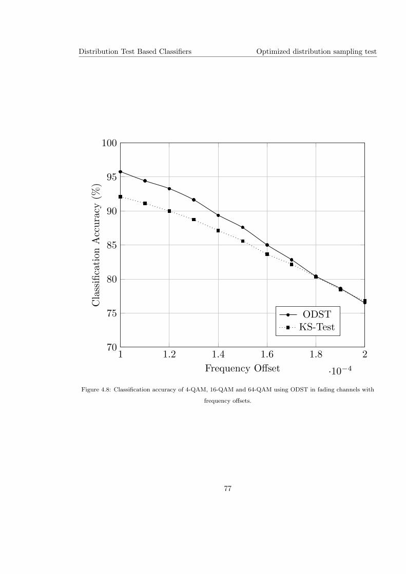
Distribution Test Based Classifiers Optimized distribution sampling test
1 1.2 1.4 1.6 1.8 2
·10−4
70
75
80
85
90
95
100
Frequency Offset
Cla
ssifi
cati
onA
ccura
cy(%
)
ODSTKS-Test
Figure 4.8: Classification accuracy of 4-QAM, 16-QAM and 64-QAM using ODST in fading channels with
frequency offsets.
77
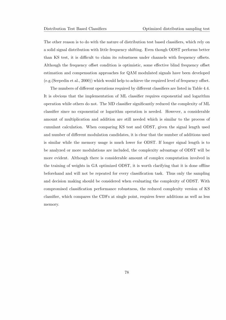
Distribution Test Based Classifiers Optimized distribution sampling test
The other reason is to do with the nature of distribution test based classifiers, which rely on
a solid signal distribution with little frequency shifting. Even though ODST performs better
than KS test, it is difficult to claim its robustness under channels with frequency offsets.
Although the frequency offset condition is optimistic, some effective blind frequency offset
estimation and compensation approaches for QAM modulated signals have been developed
(e.g.(Serpedin et al., 2000)) which would help to achieve the required level of frequency offset.
The numbers of different operations required by different classifiers are listed in Table 4.4.
It is obvious that the implementation of ML classifier requires exponential and logarithm
operation while others do not. The MD classifier significantly reduced the complexity of ML
classifier since no exponential or logarithm operation is needed. However, a considerable
amount of multiplication and addition are still needed which is similar to the process of
cumulant calculation. When comparing KS test and ODST, given the signal length used
and number of different modulation candidates, it is clear that the number of additions used
is similar while the memory usage is much lower for ODST. If longer signal length is to
be analyzed or more modulations are included, the complexity advantage of ODST will be
more evident. Although there is considerable amount of complex computation involved in
the training of weights in GA optimized ODST, it is worth clarifying that it is done offline
beforehand and will not be repeated for every classification task. Thus only the sampling
and decision making should be considered when evaluating the complexity of ODST. With
compromised classification performance robustness, the reduced complexity version of KS
classifier, which compares the CDFs at single point, requires fewer additions as well as less
memory.
78
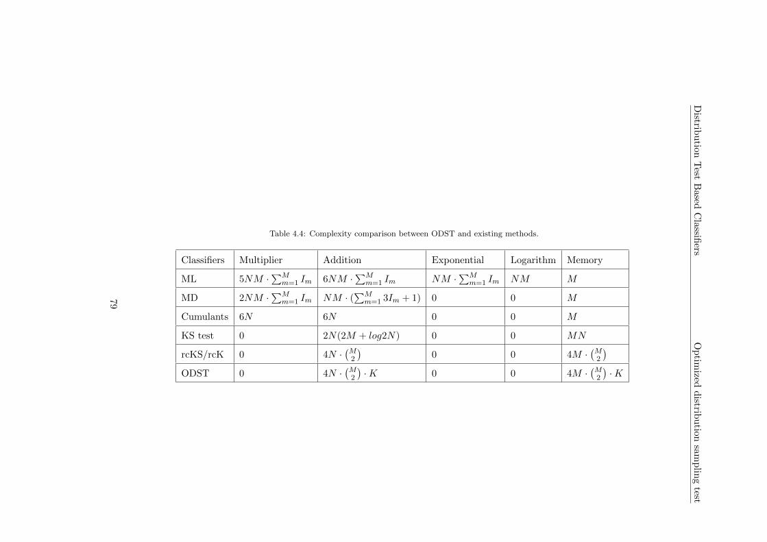
Distrib
ution
Test
Based
Classifi
ersO
ptim
izedd
istribu
tionsam
plin
gtest
Table 4.4: Complexity comparison between ODST and existing methods.
Classifiers Multiplier Addition Exponential Logarithm Memory
ML 5NM ·∑Mm=1 Im 6NM ·∑M
m=1 Im NM ·∑Mm=1 Im NM M
MD 2NM ·∑Mm=1 Im NM · (∑M
m=1 3Im + 1) 0 0 M
Cumulants 6N 6N 0 0 M
KS test 0 2N(2M + log2N) 0 0 MN
rcKS/rcK 0 4N ·(M2
)0 0 4M ·
(M2
)ODST 0 4N ·
(M2
)·K 0 0 4M ·
(M2
)·K
79
Distribution Test Based Classifiers Distribution based features
4.3 Distribution based features
The distribution based features are inspired by the ODST classifier. By treating the test
statistics sampled from different signal distributions as features, many advanced machine
learning techniques could be implemented to improve the feature enhancement and decision
making. An illustration of the overall process involved in the proposed AMC solution is
given in Figure 4.9. Different from cumulants, the proposed features are expected to be
simple to collect (low complexity), to require fewer signal samples, and to provide robustness
in different channel conditions. The proposed features are optimized for the binary classi-
fication of two modulations. To establish a low complexity classifier with reduced feature
dimension, we proposed to combine original features into new features each representing a
unique binary modulation combination for maximum separation between two modulations
using linear binomial logistic regression. The resulting class oriented features are then used
to construct a multi-dimensional feature space enabling fast classification using K-nearest
neighbour classifier. The extraction of the proposed distribution based binary discrimina-
tive features consist of two steps: optimizing sampling locations on signal distributions and
extracting the features. The extracted features are subject a further round of enhancement
using logistic regression.
In this research, we used the cumulative distribution of signals on I-Q segments (FXYM ),
amplitude (FAM ) and phase (FPM ) for analysis. Given a set of M-QAM signal r(·) of N
samples, its distributions on different signal segments can be collected using the following
equations.
FXYM (x) =1
2N
N∑n=1
{I(r′X(n) < x) + I(r′Y (n) < x)} (4.18)
FAM (x) =1
N
N∑n=1
I(| r′(n) |< x) (4.19)
FPM (x) =1
N
N∑n=1
I(arg(r′(n)) < x) (4.20)
where I(·) is a logic function which returns 1 if the input is ture and 0 if the input is false,
and arg(·) gives the phase of the complex input. An illustration of these CDFs of different
80
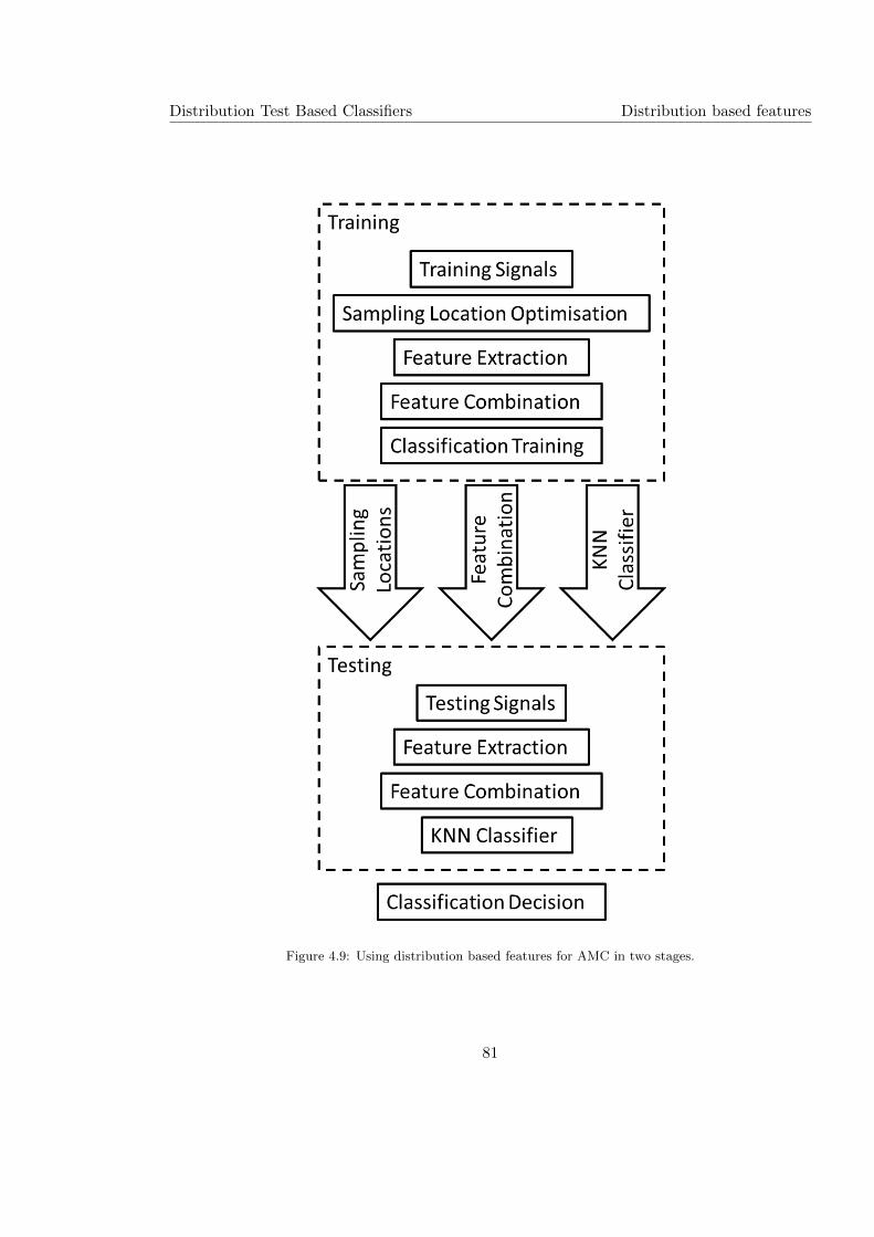
Distribution Test Based Classifiers Distribution based features
Figure 4.9: Using distribution based features for AMC in two stages.
81

Distribution Test Based Classifiers Distribution based features
signal segments are given in Figure 4.10.
4.3.1 Optimization of sampling locations
The optimization of sampling location follows the same procedure as described in Section
4.2.2. However, we extend the distribution considered to signal phase and magnitude. The
sampling location on signal distributions for feature extraction is a crucial part of the pro-
posed AMC solution. The optimization of locations should follow these criteria.
Criterion 1: The sampling locations should provide clear discrimination between two
modulations.
Criterion 2: The sampling locations should utilize a wider distribution range to provide
more comprehensive information of the modulation distribution.
Criterion 3: The locations should be at sufficient distance to avoid collecting repetitive
and redundant information.
To satisfy the above criteria, we propose to use the local maximums of the distance
between two modulations’ cumulative distributions as sampling locations. We denote D∗M1M2
to be the distance between distributions from modulations M1 and M2. “∗” is used as a
uniform representation of different signal segments including I-Q segments, amplitude and
phase.
D∗M1M2=| F ∗M1
− F ∗M2| (4.21)
The optimized sampling locations should meet the condition that the distance at location
l∗M1M2should be the maximum
D∗M1M2(l∗M1M2
) = max(D∗M1M2(x)) (4.22)
within the range of
l∗M1M2−R∗ ≤ x ≤ l∗M1M2
+R∗ (4.23)
where R∗ is a range parameter. The manually optimized values of R∗ in our simulation can
be found in Table 4.5.
82

Distribution Test Based Classifiers Distribution based features
−2.5 −2 −1.5 −1 −0.5 0 0.5 1 1.5 2 2.50
0.1
0.2
0.3
0.4
0.5
0.6
0.7
0.8
0.9
1
X ( or Y)
Cu
mu
lati
ve
Pro
ba
bil
ity
4−QAM
16−QAM
Difference (absolute)
−3 −2 −1 0 1 2 30
0.1
0.2
0.3
0.4
0.5
0.6
0.7
0.8
0.9
1
Phase
Cu
mu
lati
ve
Pro
ba
bil
ity
4−QAM
16−QAM
Difference (absolute)
0 0.5 1 1.5 2 2.5 30
0.1
0.2
0.3
0.4
0.5
0.6
0.7
0.8
0.9
1
Amplitude
Cu
mu
lati
ve
Pro
ba
bil
ity
4−QAM
16−QAM
Difference (absolute)
Figure 4.10: Cumulative Distributions of different signal segments from 4-QAM and 16-QAM at SNR of 15
dB.
83
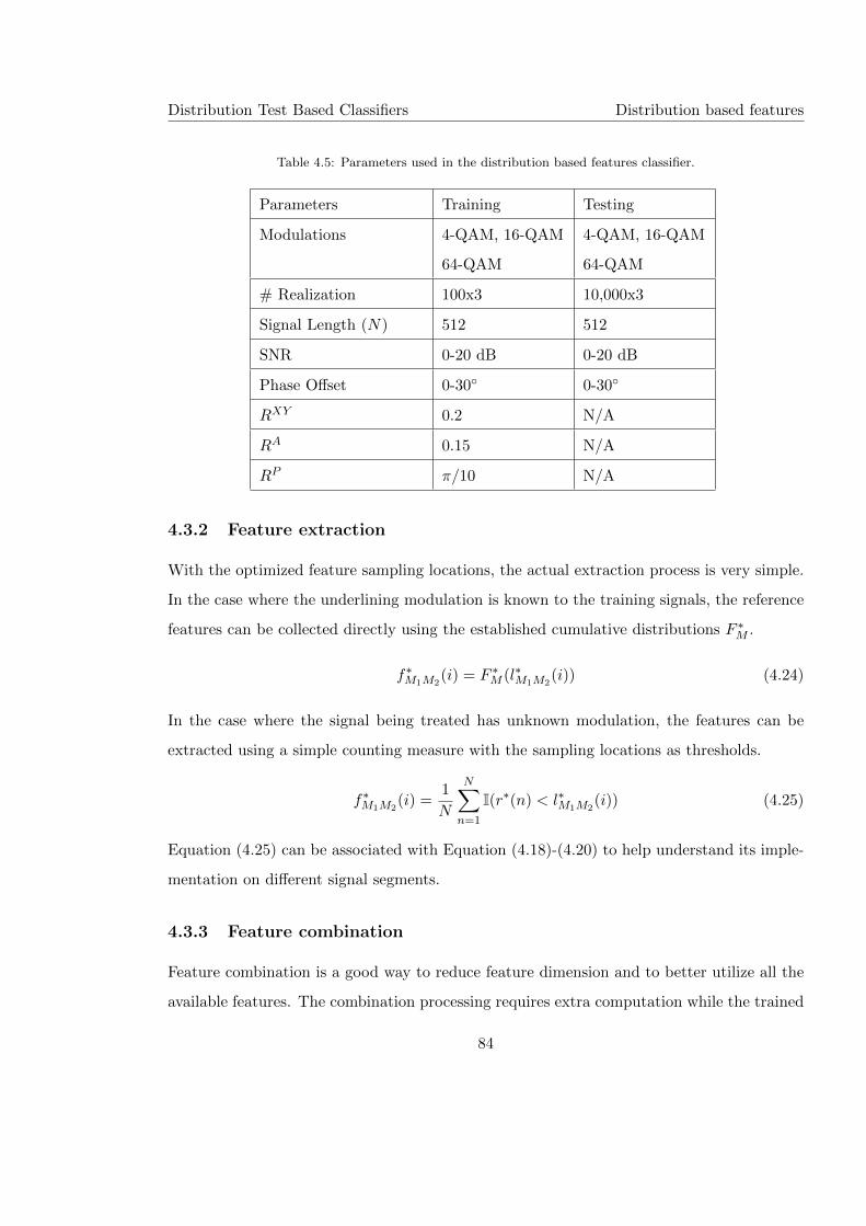
Distribution Test Based Classifiers Distribution based features
Table 4.5: Parameters used in the distribution based features classifier.
Parameters Training Testing
Modulations 4-QAM, 16-QAM
64-QAM
4-QAM, 16-QAM
64-QAM
# Realization 100x3 10,000x3
Signal Length (N) 512 512
SNR 0-20 dB 0-20 dB
Phase Offset 0-30◦ 0-30◦
RXY 0.2 N/A
RA 0.15 N/A
RP π/10 N/A
4.3.2 Feature extraction
With the optimized feature sampling locations, the actual extraction process is very simple.
In the case where the underlining modulation is known to the training signals, the reference
features can be collected directly using the established cumulative distributions F ∗M .
f∗M1M2(i) = F ∗M (l∗M1M2
(i)) (4.24)
In the case where the signal being treated has unknown modulation, the features can be
extracted using a simple counting measure with the sampling locations as thresholds.
f∗M1M2(i) =
1
N
N∑n=1
I(r∗(n) < l∗M1M2(i)) (4.25)
Equation (4.25) can be associated with Equation (4.18)-(4.20) to help understand its imple-
mentation on different signal segments.
4.3.3 Feature combination
Feature combination is a good way to reduce feature dimension and to better utilize all the
available features. The combination processing requires extra computation while the trained
84
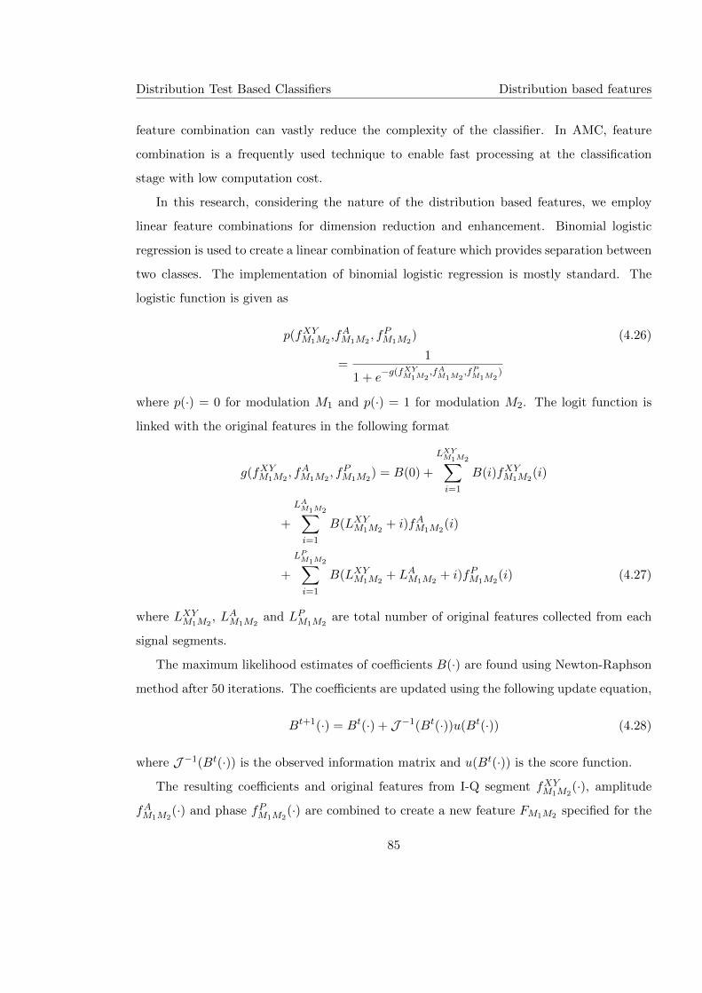
Distribution Test Based Classifiers Distribution based features
feature combination can vastly reduce the complexity of the classifier. In AMC, feature
combination is a frequently used technique to enable fast processing at the classification
stage with low computation cost.
In this research, considering the nature of the distribution based features, we employ
linear feature combinations for dimension reduction and enhancement. Binomial logistic
regression is used to create a linear combination of feature which provides separation between
two classes. The implementation of binomial logistic regression is mostly standard. The
logistic function is given as
p(fXYM1M2,fAM1M2
, fPM1M2) (4.26)
=1
1 + e−g(fXYM1M2
,fAM1M2,fPM1M2
)
where p(·) = 0 for modulation M1 and p(·) = 1 for modulation M2. The logit function is
linked with the original features in the following format
g(fXYM1M2, fAM1M2
, fPM1M2) = B(0) +
LXYM1M2∑i=1
B(i)fXYM1M2(i)
+
LAM1M2∑i=1
B(LXYM1M2+ i)fAM1M2
(i)
+
LPM1M2∑i=1
B(LXYM1M2+ LAM1M2
+ i)fPM1M2(i) (4.27)
where LXYM1M2, LAM1M2
and LPM1M2are total number of original features collected from each
signal segments.
The maximum likelihood estimates of coefficients B(·) are found using Newton-Raphson
method after 50 iterations. The coefficients are updated using the following update equation,
Bt+1(·) = Bt(·) + J −1(Bt(·))u(Bt(·)) (4.28)
where J −1(Bt(·)) is the observed information matrix and u(Bt(·)) is the score function.
The resulting coefficients and original features from I-Q segment fXYM1M2(·), amplitude
fAM1M2(·) and phase fPM1M2
(·) are combined to create a new feature FM1M2 specified for the
85
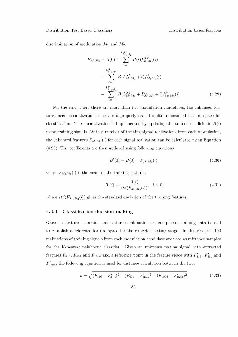
Distribution Test Based Classifiers Distribution based features
discrimination of modulation M1 and M2.
FM1M2 = B(0) +
LXYM1M2∑i=1
B(i)fXYM1M2(i)
+
LAM1M2∑i=1
B(LXYM1M2+ i)fAM1M2
(i)
+
LPM1M2∑i=1
B(LXYM1M2+ LAM1M2
+ i)fPM1M2(i) (4.29)
For the case where there are more than two modulation candidates, the enhanced fea-
tures need normalization to create a properly scaled multi-dimensional feature space for
classification. The normalization is implemented by updating the trained coefficients B(·)using training signals. With a number of training signal realizations from each modulation,
the enhanced features FM1M2(·) for each signal realization can be calculated using Equation
(4.29). The coefficients are then updated using following equations.
B′(0) = B(0)− FM1M2(·) (4.30)
where FM1M2(·) is the mean of the training features,
B′(i) =B(i)
std(FM1M2(·)) , i > 0 (4.31)
where std(FM1M2(·)) gives the standard deviation of the training features.
4.3.4 Classification decision making
Once the feature extraction and feature combination are completed, training data is used
to establish a reference feature space for the expected testing stage. In this research 100
realizations of training signals from each modulation candidate are used as reference samples
for the K-nearest neighbour classifier. Given an unknown testing signal with extracted
features F416, F464 and F1664 and a reference point in the feature space with F ′416, F ′464 and
F ′1664, the following equation is used for distance calculation between the two,
d =√
(F416 − F ′416)2 + (F464 − F ′464)2 + (F1664 − F ′1664)2 (4.32)
86

Distribution Test Based Classifiers Distribution based features
−2 −1.5 −1 −0.5 0 0.5 1 1.50
0.02
0.04
0.06
0.08
0.1
F416
Probability
4−QAM
16−QAM
64−QAM
(a) F416 for 4-QAM and 16-QAM discrimination
−2 −1.5 −1 −0.5 0 0.5 1 1.50
0.01
0.02
0.03
0.04
0.05
0.06
0.07
0.08
F464
Pro
bability
4−QAM
16−QAM
64−QAM
(b) F464 for 4-QAM and 64-QAM discrimination
−4 −3 −2 −1 0 1 2 3 40
0.01
0.02
0.03
0.04
0.05
0.06
0.07
F1664
Pro
bability
4−QAM
16−QAM
64−QAM
(c) F1664 for 16-QAM and 64-QAM discrimination
Figure 4.11: Enhanced distribution based features and their distribution projection on each separate
dimension.
87
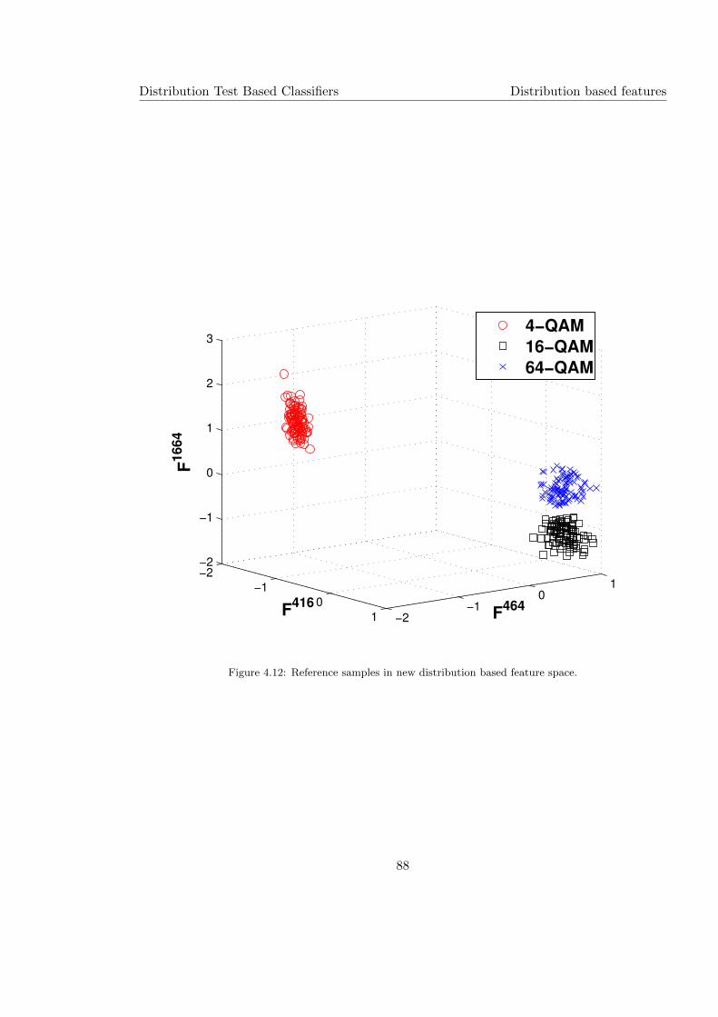
Distribution Test Based Classifiers Distribution based features
−2
−1
0
1 −2
−1
0
1
−2
−1
0
1
2
3
F464F
416
F1664
4−QAM
16−QAM
64−QAM
Figure 4.12: Reference samples in new distribution based feature space.
88
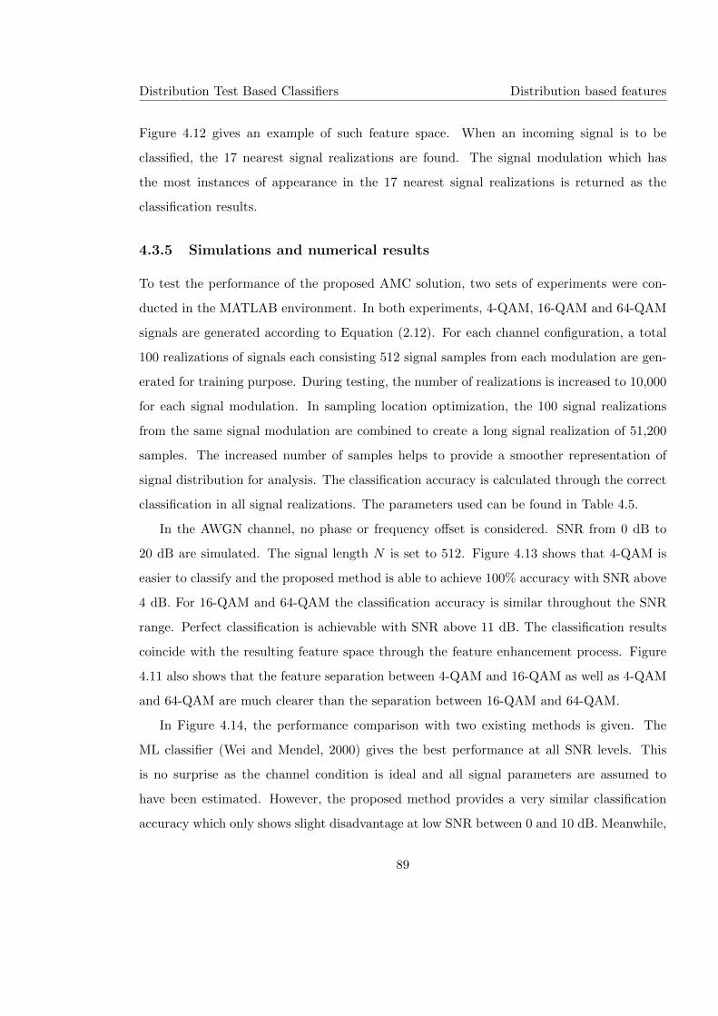
Distribution Test Based Classifiers Distribution based features
Figure 4.12 gives an example of such feature space. When an incoming signal is to be
classified, the 17 nearest signal realizations are found. The signal modulation which has
the most instances of appearance in the 17 nearest signal realizations is returned as the
classification results.
4.3.5 Simulations and numerical results
To test the performance of the proposed AMC solution, two sets of experiments were con-
ducted in the MATLAB environment. In both experiments, 4-QAM, 16-QAM and 64-QAM
signals are generated according to Equation (2.12). For each channel configuration, a total
100 realizations of signals each consisting 512 signal samples from each modulation are gen-
erated for training purpose. During testing, the number of realizations is increased to 10,000
for each signal modulation. In sampling location optimization, the 100 signal realizations
from the same signal modulation are combined to create a long signal realization of 51,200
samples. The increased number of samples helps to provide a smoother representation of
signal distribution for analysis. The classification accuracy is calculated through the correct
classification in all signal realizations. The parameters used can be found in Table 4.5.
In the AWGN channel, no phase or frequency offset is considered. SNR from 0 dB to
20 dB are simulated. The signal length N is set to 512. Figure 4.13 shows that 4-QAM is
easier to classify and the proposed method is able to achieve 100% accuracy with SNR above
4 dB. For 16-QAM and 64-QAM the classification accuracy is similar throughout the SNR
range. Perfect classification is achievable with SNR above 11 dB. The classification results
coincide with the resulting feature space through the feature enhancement process. Figure
4.11 also shows that the feature separation between 4-QAM and 16-QAM as well as 4-QAM
and 64-QAM are much clearer than the separation between 16-QAM and 64-QAM.
In Figure 4.14, the performance comparison with two existing methods is given. The
ML classifier (Wei and Mendel, 2000) gives the best performance at all SNR levels. This
is no surprise as the channel condition is ideal and all signal parameters are assumed to
have been estimated. However, the proposed method provides a very similar classification
accuracy which only shows slight disadvantage at low SNR between 0 and 10 dB. Meanwhile,
89
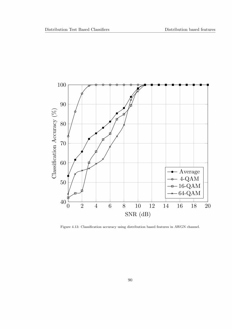
Distribution Test Based Classifiers Distribution based features
0 2 4 6 8 10 12 14 16 18 2040
50
60
70
80
90
100
SNR (dB)
Cla
ssifi
cati
onA
ccura
cy(%
)
Average4-QAM16-QAM64-QAM
Figure 4.13: Classification accuracy using distribution based features in AWGN channel.
90
Distribution Test Based Classifiers Distribution based features
the cumulant based Genetic Programming classifier (Aslam et al., 2012) suffers from the low
signal length (N = 512) used and gives much low accuracy even with high SNR levels.
0 2 4 6 8 10 12 14 16 18 2050
60
70
80
90
100
SNR (dB)
Cla
ssifi
cati
onA
ccura
cy(%
)
This researchML
GP-cumulants
Figure 4.14: Averaged classification accuracy using different classifiers in AWGN channel.
Another common channel condition is carrier phase offset. In this experiment, we simu-
lated the carrier phase offset of 0◦ to 30◦. Other channel conditions are set to the same as
the previous experiments with SNR of 10 dB and signal length of 512. Figure 4.15 shows the
resulting classification accuracy for three classifiers with different degrees of carrier phase
offset. ML classifier achieves the best accuracy with no or little phase offset. Meanwhile,
the Kolmogorov Smirnov test classifier (Wang and Wang, 2010) is severely affected by the
increasing amount of phase offset. Having similar classification accuracy with little carrier
91
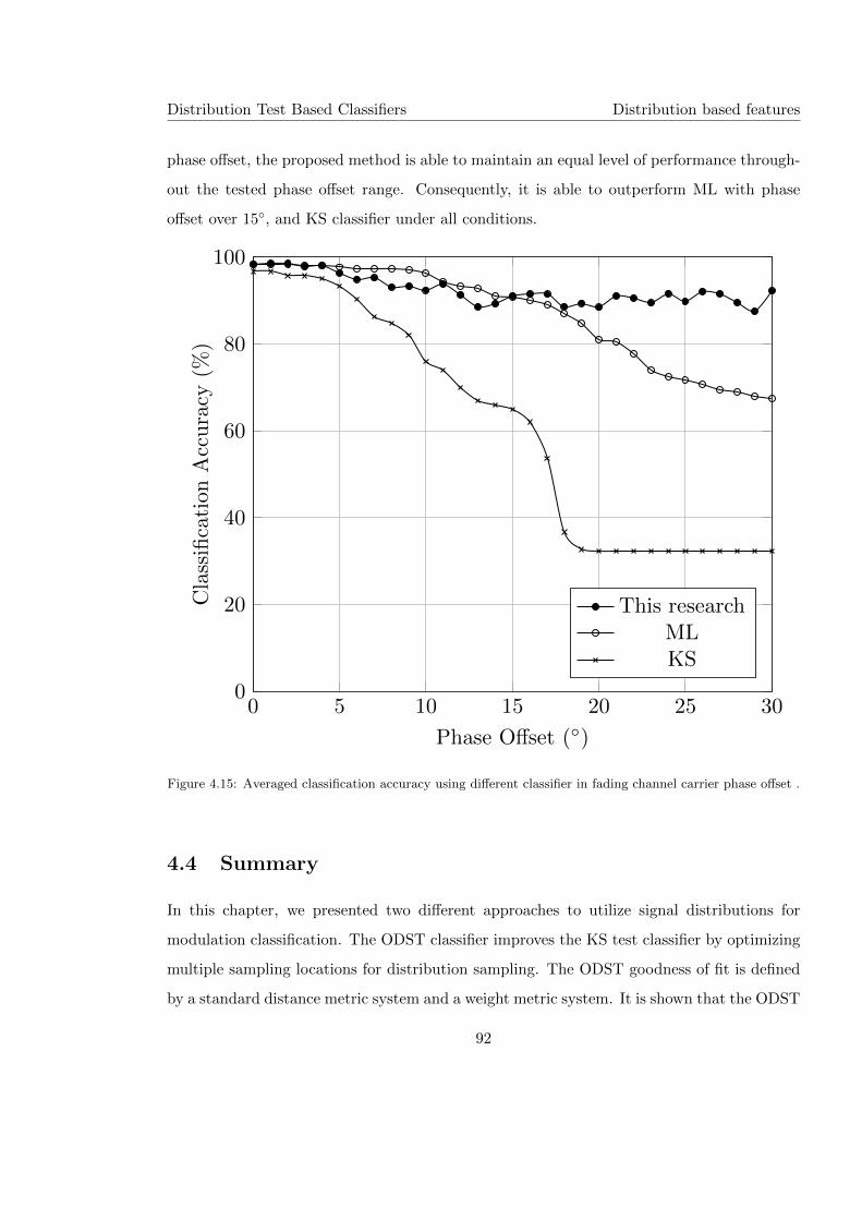
Distribution Test Based Classifiers Distribution based features
phase offset, the proposed method is able to maintain an equal level of performance through-
out the tested phase offset range. Consequently, it is able to outperform ML with phase
offset over 15◦, and KS classifier under all conditions.
0 5 10 15 20 25 300
20
40
60
80
100
Phase Offset (◦)
Cla
ssifi
cati
onA
ccura
cy(%
)
This researchMLKS
Figure 4.15: Averaged classification accuracy using different classifier in fading channel carrier phase offset .
4.4 Summary
In this chapter, we presented two different approaches to utilize signal distributions for
modulation classification. The ODST classifier improves the KS test classifier by optimizing
multiple sampling locations for distribution sampling. The ODST goodness of fit is defined
by a standard distance metric system and a weight metric system. It is shown that the ODST
92
Distribution Test Based Classifiers Distribution based features
classifier is superior to cumulant based classifier who is subject to sever degradation with
limited signal length. In addition, the optimization of weights using GA is able to further
improve the classification accuracy by a small margin. In another approach, the sampled
signal distribution values are treated as features. By extending the signal distributions into
phase and magnitude, more features are available for analysis. The dimension reduction
problem is solved by a logistic regression process where features combined into smaller new
feature sets. The resulting classifier show superior performance in complex channel with
phase offset.
93
Chapter 5
Modulation Classification with
Unknown Noise
5.1 Introduction
As discussed in Chapter 2, most of the existing modulation classifiers require the knowledge
of noise model and noise power to achieve modulation classifications. Likelihood based
classifiers promise optimal classification accuracy (Wei and Mendel, 2000; Gao et al., 2008;
Hameed et al., 2009; Xu et al., 2011; Shi and Karasawa, 2011, 2012). Unfortunately, such
method requires a matching channel model as well as perfect knowledge of channel parameters
to achieve optimality. Efforts have been made to relax some of the rules serving an optimal
LB classifier. Wong and Nandi (Wong and Nandi, 2008) suggested a semi-blind LB classifier
with carrier phase and noise power estimation in a non-coherent environment. Panagiotou
et al. (Panagiotou et al., 2000) employ GLRT and Hybrid likelihood ratio test HLRT to
achieve classification with carrier phase as unknown parameters. Huang and Polydoros
(Huang and Polydoros, 1995) presented the quasi-Log-Likelihood Ratio Test (qLLRT) with
carrier phase as unknown parameter. All these likelihood based semi-blind classifiers mitigate
the dependence on one or two channel parameters. None offers the ability of classification in
a completely blind environment. Another new branch of decision theoretic methods employs
94

Modulation Classification with Unknown Noise Introduction
distribution test for low complexity modulation classification (Wang and Wang, 2010; Urriza
et al., 2011; Zhu et al., 2013a). Yet, all channel parameters are assumed to be available.
Feature based methods often provide near-optimal performance with lower complexity.
The extraction of most features do not require channel parameters such a channel gain, car-
rier phase offset, or noise variance. However, they are often acquired for the optimization
of decision thresholds and reference values. Nandi and Azzouz (Nandi and Azzouz, 1998)
used spectral-based feature sets for effective classification of digital modulations. Cumu-
lant features suggested by Swami and Saddler (Swami and Sadler, 2000) became popular
for the classification of digital modulations with different orders (Wu et al., 2008). Cyclic
features are another set of features for modulation classification which exploits the cyclo-
stationarity of the signals (Gardner and Spooner, 1992; Punchihewa et al., 2010). Lately,
machine learning techniques have become a new trend for feature based methods. Wong and
Nandi suggested artificial neural network and genetic algorithm for feature combination and
dimension reduction (Wong and Nandi, 2004). Genetic Programming is another advanced
machine learning algorithm to provide improved performance (Aslam et al., 2012). Despite
their robust performance, all feature based methods require channel parameters to achieve
high classification accuracy.
For the purpose of complete blind classification, we propose two centroid estimator for
the joint estimation of channel gain and carrier phase. A new non-parametric likelihood
function is proposed as a low complexity alternative which aims to serve a wider variety of
channel conditions. Figure 5.1 provides an overview of the implementation of the proposed
blind modulation classier for M-ary PSK and QAM.
95
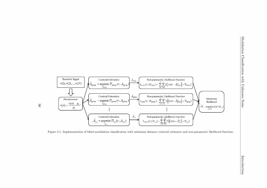
Mod
ula
tionC
lassifica
tionw
ithU
nkn
own
Noise
Intro
du
ction
Figure 5.1: Implementation of blind modulation classification with minimum distance centroid estimator and non-parametric likelihood function.
96

Modulation Classification with Unknown Noise Centroid estimation
5.2 Classification strategy
Given a set of candidate modulations M, the classification decision M is drawn from the
hypothesis models HM of modulation M∈M with a maximum likelihood L(r|HM)
M = argmaxM∈M
L(r|HM) (5.1)
Most classifiers require the prior knowledge of the channel gain α, carrier phase θ, mod-
ulation symbols sM, and noise σ variance before the test could be conducted. In addition,
in many cases, the parameters are considered identical among different hypothesis models
with the exception of modulation symbols.
L(r|HM) = L(r|α, θ, sM, σ) (5.2)
In the case of blind modulation classification, parameters have to be estimated. The
estimation is likely to differ among different hypothesis models, as it is natural to estimate
the parameters with the assumption of modulation type to achieve more accurate likelihood
evaluation.
L(r|HM) = L(r|αM, θM, sM, σM) (5.3)
To reduced complexity of estimating multiple interlinked parameters, we suggest treating
noise variance as unknown parameters and employ alternative likelihood functions to mitigate
its necessity.
L(r|HM) = L(r|αM, θM, sM) (5.4)
The estimations of channel gain and carrier phase are combined as the estimation of received
signal centroids AMAM = αMe
jθMsM (5.5)
reducing the estimation task to a single parameter and the likelihood function to be related
to only the signal centroids.
L(r|HM) = L(r|AM) (5.6)
We will start the discussion with the estimation of signal centroids AM and then progress
to the likelihood functions in later sections.
97
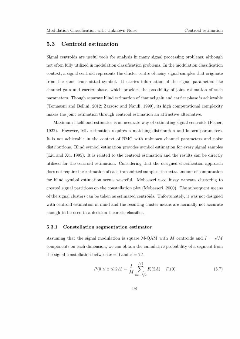
Modulation Classification with Unknown Noise Centroid estimation
5.3 Centroid estimation
Signal centroids are useful tools for analysis in many signal processing problems, although
not often fully utilized in modulation classification problems. In the modulation classification
context, a signal centroid represents the cluster centre of noisy signal samples that originate
from the same transmitted symbol. It carries information of the signal parameters like
channel gain and carrier phase, which provides the possibility of joint estimation of such
parameters. Though separate blind estimation of channel gain and carrier phase is achievable
(Tomasoni and Bellini, 2012; Zarzoso and Nandi, 1999), its high computational complexity
makes the joint estimation through centroid estimation an attractive alternative.
Maximum likelihood estimator is an accurate way of estimating signal centroids (Fisher,
1922). However, ML estimation requires a matching distribution and known parameters.
It is not achievable in the context of BMC with unknown channel parameters and noise
distributions. Blind symbol estimation provides symbol estimation for every signal samples
(Liu and Xu, 1995). It is related to the centroid estimation and the results can be directly
utilized for the centroid estimation. Considering that the designed classification approach
does not require the estimation of each transmitted samples, the extra amount of computation
for blind symbol estimation seems wasteful. Mobasseri used fuzzy c-means clustering to
created signal partitions on the constellation plot (Mobasseri, 2000). The subsequent means
of the signal clusters can be taken as estimated centroids. Unfortunately, it was not designed
with centroid estimation in mind and the resulting cluster means are normally not accurate
enough to be used in a decision theoretic classifier.
5.3.1 Constellation segmentation estimator
Assuming that the signal modulation is square M-QAM with M centroids and I =√M
components on each dimension, we can obtain the cumulative probability of a segment from
the signal constellation between x = 0 and x = 2A
P (0 ≤ x ≤ 2A) =I
M
I/2∑i=−I/2
Fi(2A)− Fi(0) (5.7)
98
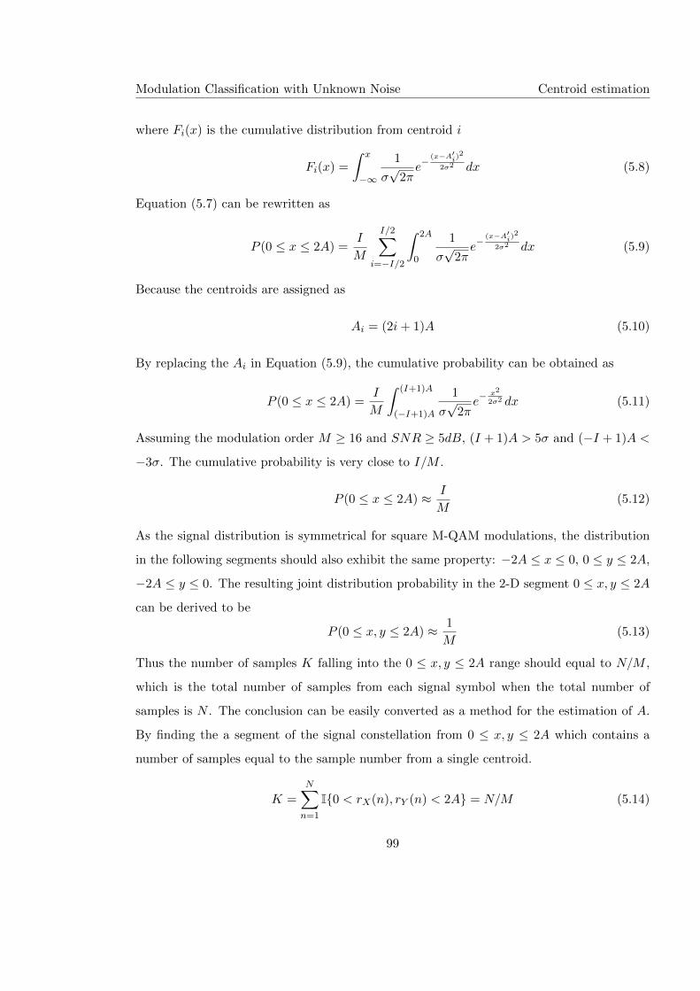
Modulation Classification with Unknown Noise Centroid estimation
where Fi(x) is the cumulative distribution from centroid i
Fi(x) =
∫ x
−∞
1
σ√
2πe−
(x−A′i)2
2σ2 dx (5.8)
Equation (5.7) can be rewritten as
P (0 ≤ x ≤ 2A) =I
M
I/2∑i=−I/2
∫ 2A
0
1
σ√
2πe−
(x−A′i)2
2σ2 dx (5.9)
Because the centroids are assigned as
Ai = (2i+ 1)A (5.10)
By replacing the Ai in Equation (5.9), the cumulative probability can be obtained as
P (0 ≤ x ≤ 2A) =I
M
∫ (I+1)A
(−I+1)A
1
σ√
2πe−
x2
2σ2 dx (5.11)
Assuming the modulation order M ≥ 16 and SNR ≥ 5dB, (I + 1)A > 5σ and (−I + 1)A <
−3σ. The cumulative probability is very close to I/M .
P (0 ≤ x ≤ 2A) ≈ I
M(5.12)
As the signal distribution is symmetrical for square M-QAM modulations, the distribution
in the following segments should also exhibit the same property: −2A ≤ x ≤ 0, 0 ≤ y ≤ 2A,
−2A ≤ y ≤ 0. The resulting joint distribution probability in the 2-D segment 0 ≤ x, y ≤ 2A
can be derived to be
P (0 ≤ x, y ≤ 2A) ≈ 1
M(5.13)
Thus the number of samples K falling into the 0 ≤ x, y ≤ 2A range should equal to N/M ,
which is the total number of samples from each signal symbol when the total number of
samples is N . The conclusion can be easily converted as a method for the estimation of A.
By finding the a segment of the signal constellation from 0 ≤ x, y ≤ 2A which contains a
number of samples equal to the sample number from a single centroid.
K =N∑n=1
I{0 < rX(n), rY (n) < 2A} = N/M (5.14)
99
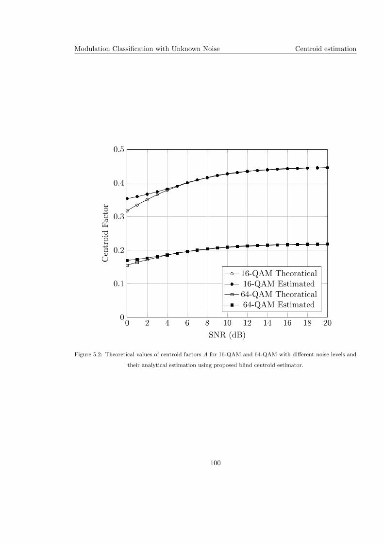
Modulation Classification with Unknown Noise Centroid estimation
0 2 4 6 8 10 12 14 16 18 200
0.1
0.2
0.3
0.4
0.5
SNR (dB)
CentroidFactor
16-QAM Theoratical16-QAM Estimated64-QAM Theoratical64-QAM Estimated
Figure 5.2: Theoretical values of centroid factors A for 16-QAM and 64-QAM with different noise levels and
their analytical estimation using proposed blind centroid estimator.
100
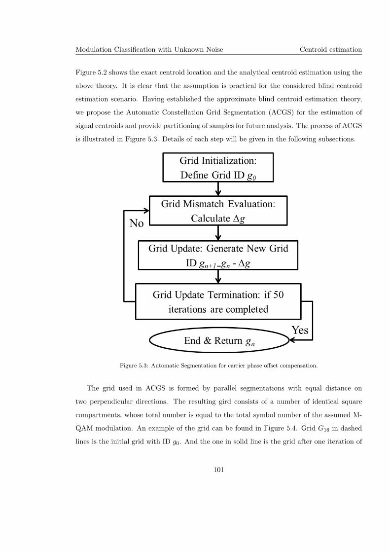
Modulation Classification with Unknown Noise Centroid estimation
Figure 5.2 shows the exact centroid location and the analytical centroid estimation using the
above theory. It is clear that the assumption is practical for the considered blind centroid
estimation scenario. Having established the approximate blind centroid estimation theory,
we propose the Automatic Constellation Grid Segmentation (ACGS) for the estimation of
signal centroids and provide partitioning of samples for future analysis. The process of ACGS
is illustrated in Figure 5.3. Details of each step will be given in the following subsections.
Figure 5.3: Automatic Segmentation for carrier phase offset compensation.
The grid used in ACGS is formed by parallel segmentations with equal distance on
two perpendicular directions. The resulting gird consists of a number of identical square
compartments, whose total number is equal to the total symbol number of the assumed M-
QAM modulation. An example of the grid can be found in Figure 5.4. Grid G16 in dashed
lines is the initial grid with ID g0. And the one in solid line is the grid after one iteration of
101
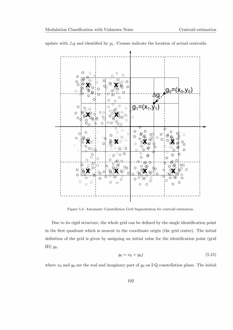
Modulation Classification with Unknown Noise Centroid estimation
update with 4g and identified by g1. Crosses indicate the location of actual centroids.
g0=(x0,y0)
g1=(x1,y1)
∆g
x x
x x
x x
x x
x
x
x
x
Figure 5.4: Automatic Constellation Grid Segmentation for centroid estimation.
Due to its rigid structure, the whole grid can be defined by the single identification point
in the first quadrant which is nearest to the coordinate origin (the grid centre). The initial
definition of the grid is given by assigning an initial value for the identification point (grid
ID) g0.
g0 = x0 + y0j (5.15)
where x0 and y0 are the real and imaginary part of g0 on I-Q constellation plane. The initial
102
Modulation Classification with Unknown Noise Centroid estimation
values of x0 and y0 are set to the same. A mathematical expression of grid junctions GM
can be found in Equation (5.16).
GM =
− I2y + I
2xj · · · −y + I2xj x+ I
2yj · · · I2x+ I
2yj...
......
...
− I2y + xj · · · −y + x0j x+ yj · · · I
2x+ yj
− I2x− yj · · · −x− yj y − xj · · · I
2y − xj...
......
...
− I2x− I
2yj · · · −x− I2yj y − I
2xj · · · I2y − I
2xj
(5.16)
By updating the grid, the end results of ACGS should produce a grid which fits the
pattern of the centroid distribution. The centre of each partition (square compartment)
on the grid should be aligned to the corresponding centroid from the modulated signal. A
definition of the grid partition centres SM for M-QAM modulation is given in Equation
(5.17).
SM =
(1+I/2)(−y+xj)2 · · · −y
2 + (1+I/2)x2 j x
2 + (1+I/2)y2 j · · · (1+I/2)(x+yj)
2...
......
...
− (1+I/2)y2 + x
2 j · · · −y2 + x
2 jx2 + y
2j · · · (1+I/2)x2 + y
2j
− (1+I/2)x2 − y
2j · · · −x2 −
y2j
y2 − x
2 j · · · (1+I/2)y2 − x
2 j...
......
...
(1+I/2)(−x−yj)2 · · · −x
2 −(1+I/2)y
2 j y2 −
(1+I/2)x2 j · · · (1+I/2)(y−xj)
2
(5.17)
Having calculated the error, the grid is updated using the following equation.
gn+1 = (xn −4g) + (yn −4g)j (5.18)
The grid update process is repeated for 50 iterations. After the last iteration, the final
grid and signal partitioning are returned for use in the actual modulation classification. The
returned grid ID point g′ = x′+ y′j will be used to form the complete grid matrix as well as
centroid matrix.
In the case where there is carrier phase offset θ0, the grid is first trained to compensate
the phase error. It is accomplished with a phase error function and a grid update function.
4θ = θg − θl (5.19)
103
Modulation Classification with Unknown Noise Centroid estimation
where θg is the phase of the grid defined by the grid ID gn
θg = arg(gn) (5.20)
and θl is the average phase of all samples in partition 1 in the 1st quadrant.
θl = arg{r′(ln = 1)} (5.21)
The grid will then be updated using the following equation
gn+1 =| gn | ej(θg−4θ) (5.22)
The training will be repeated for 50 iterations and the the final θg will be returned as the
estimated carrier phase offset θ′. To compensate the phase offset, Equation (5.15) and (5.18)
used in ACGS should be modified to the following two equations
g0 =| x0 + y0j | ejθ′
(5.23)
gn+1 = {xn − cos(θ′)4 g}+ {yn − sin(θ′)4 g}j (5.24)
5.3.2 Minimum distance estimator
Through ACGS, signal centroids can be estimated for square M-QAM modulation signals.
However, it is not able to perform centroid estimation for other digital modulations and to
assist the classification of these modulations. For this reason, we have developed a different
estimation approach named Minimum Distance Centroid Estimator (MDCE). The notion is
to define a set of signal centroids that are intended to indicate the modulation symbol after
communication channel without the additive noises.
We assume that the estimated centroids AM to possess the original rigid structure after
transmission and pre-processing. The mean of centroids µ(AM) should remain at 0, the
magnitude of two different centroid elements ApM and AqM should follow the original pro-
portion∥∥ApM∥∥ /∥∥AqM∥∥ =
∥∥spM∥∥ / ∥∥sqM∥∥, and the phase difference between centroids should
remain the same φ(ApM) − φ(AqM) = φ(spM) − φ(sqM). The resulting expression for sets of
104
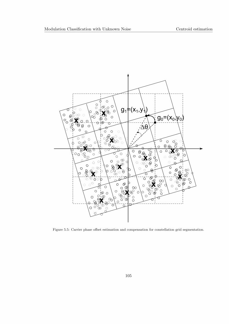
Modulation Classification with Unknown Noise Centroid estimation
g0=(x0,y0)g1=(x1,y1)
∆θx
x
x
x
xx
xx
x
x
x
x
Figure 5.5: Carrier phase offset estimation and compensation for constellation grid segmentation.
105

Modulation Classification with Unknown Noise Centroid estimation
centroids for BPSK, QPSK/4-QAM and 8-PSK can be expressed in a simplified form with
a single centroid parameter A = aeiφs0M.
ABPSK =[−A A
](5.25)
AQPSK = A4−QAM =
jA A
−A −jA
(5.26)
A8−PSK =
−jA jA∗
−A∗ A
A A∗
−jA∗ jA
(5.27)
Therefore the estimation of AM can be reduced to the estimation of the centroid param-
eter A. The reference symbol s0M is defined as the one which is nearest to the signal mean.
The expressions of signal centroid for 16-QAM and 64-QAM modulations are not given here
due to their large size and relative ease to derive with the given rules.
To measure the mismatch between the observed signal and the potential centroids esti-
mation, a signal-to-centroid distance is designed to accomplish the task. With no assumption
of the noise variance and distribution, we propose the overall distance DM(r,AM) to be the
sum of the Euclidean distance between each signal sample and its nearest centroid
DM(r ,AM) =N∑n=1
minm∈[1,..,M ]
(‖r(n)−AmM‖) (5.28)
where M is the total number of centroids in the centroid collection AM.
Such distance metric was first proposed by Wong and Nandi in (Wong and Nandi, 2008),
where it is used as a model mismatch evaluation for a minimum distance classifier. As a
classifier, the distance metric always produce shorter distance for higher order modulations
which leads to a bias in classification for higher order modulations. However, such problem
does not existence in centroid estimation, as it is conducted within a modulation hypothesis
and the mismatch is only caused by the estimated centroids of the same order.
106

Modulation Classification with Unknown Noise Non-parametric likelihood function
The signal centroids AM are estimated by finding the minimum of the distance metrics
DM(r ,AM).
AM = arg minAM
DM(r ,AM) (5.29)
For the estimator to be valid, the expectation of the estimated centroids E[AM] should
equal to αejθsM with the channel gain α, the carrier phase θ, and the transmitted symbols
sM. The estimation of the centroids is a solutions of the derivative of the signal-to-centroid
distance expectation ∂∂AME[DM(r,AM)] = 0. Replace the centroids with the single centroid
parameter A = aeiφs0M. The analysis can be divided into a = α when ∂
∂aE[DM(r, a)] = 0,
and φ = θ when ∂∂φE[DM(r, φ)] = 0. The detailed proof is given in Appendix A.
The implementation of MDCE is realized by an iterative sub-gradient optimization pro-
cess. The details are given in Appendix B.
The estimator is tested in the simulated AWGN channel at different SNR levels from 0
dB to 20 dB. At each noise level, 1,000 signal realizations are tested with each consisting
N=1,024 samples. In Figure 5.6, it is clear that the centroid estimator provides a very
accurate estimation of the channel gain with a very small amount of deviation at SNR over
10 dB. The accuracy degrades with increased level of noise and a quick acceleration is seen
at SNR below 5 dB. Since the estimator of centroid magnitude relies on the approximation
of the Rice distribution to a normal distribution as described in Appendix A, the estimation
of the 8-PSK centroid magnitude receives a more significant impact than 16-QAM despite
having a lower order. I believe the multiple layers of centroids with different magnitudes in
16-QAM help to compensate the biased estimation error caused by the approximation. It is
worth noting that the The phase error in Figure 5.7 tells a similar story. The influence of
the estimation error in the classification performance will be discussed in Section 5.5.
5.4 Non-parametric likelihood function
To enable likelihood evaluation without known noise model and power, we propose a new
low complexity non-parametric likelihood function. Firstly, we relax the assumption of noise
distribution to be any symmetrical distribution with higher density at signal mean. Secondly,
107
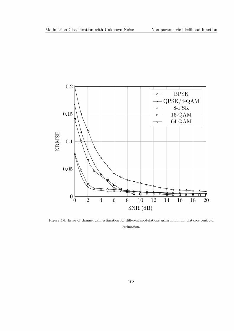
Modulation Classification with Unknown Noise Non-parametric likelihood function
0 2 4 6 8 10 12 14 16 18 200
0.05
0.1
0.15
0.2
SNR (dB)
NRMSE
BPSK
QPSK/4-QAM8-PSK16-QAM64-QAM
Figure 5.6: Error of channel gain estimation for different modulations using minimum distance centroid
estimation.
108
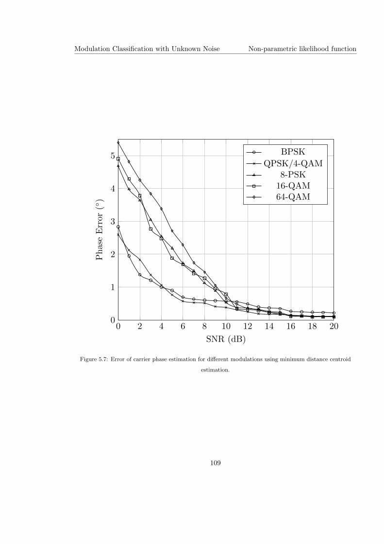
Modulation Classification with Unknown Noise Non-parametric likelihood function
0 2 4 6 8 10 12 14 16 18 200
1
2
3
4
5
SNR (dB)
PhaseError
(◦)
BPSK
QPSK/4-QAM8-PSK16-QAM64-QAM
Figure 5.7: Error of carrier phase estimation for different modulations using minimum distance centroid
estimation.
109
Modulation Classification with Unknown Noise Non-parametric likelihood function
we replace the noise variance by an expression of the estimated channel gain and estimated
centroids numbers. Thirdly, we reduce logarithm operation of likelihood calculation to simple
counting operation. The resulting likelihood function can be found as
LNP (r|HM) =
N∑n=1
M∑m=1
I{∥∥∥r(n)− A(m)
M
∥∥∥ < RM} (5.30)
where I(.) is a conditional function which returns 1 if the input is true and 0 if input is false,
and the radius parameter RM is given by
RM = R0/√M. (5.31)
The selection of the reference radius R0 will be discussed in later part of this section.
The non-parametric likelihood function is effectively an estimation of the cumulative
probability of the given signal in a set of defined local regions. The expectation of the
likelihood can be expressed in the following manner.
E[LNPLF (r|HM)] =
∫SM
f(x, y)dS (5.32)
where SM is a limit associated with estimated centroids AM and the test radius RM, and
f(x, y) is the PDF of the testing signal.
f(x, y) =1
M
M∑m=1
1
σ√
2πe−
(x−<(αejθsmM))2+(y−=(αejθsmM))
2
2σ2 (5.33)
It is easy to see that, with the given testing radius, the area of SM = M ·πR20/M = πR2
0
is designed to given each hypothesis equal area for the cumulative probability calculation.
The decision is based on the assumption that matching model should provide maximum
cumulative probability in defined regions of the same total area.
M = argmaxM∈M
∫SM
f(x, y)dS (5.34)
Without examining the centroid estimation for false hypothesis modulations, we evaluate
the maximum non-parametric likelihood of different hypothesis in the scenario where each set
of estimated centroids have the maximum number of overlaps with the true signal centroids.
Such a scenario has been previously examined for the GLRT classifier with unknown channel
110

Modulation Classification with Unknown Noise Simulations and numerical results
gain and carrier phase which results in equal likelihood for nested modulations at high SNR
(Panagiotou et al., 2000). Approximating the signal distribution at each transmitted signal
symbol to a Rayleigh distribution,
f(R) =Rσ2e−R
2/2σ2(5.35)
the likelihood function estimation become a function of the testing radius.
E[LNPLF (r|HM)] = NM
RM∫0
x
σ2e−x
2/2σ2dx (5.36)
where NM is the maximum number of matching centroids for the hypothesisM. For example,
given a piece of QPSK signal, the value of NM for different hypothesises would be: NBPSK =
2, NQPSK = 4 and N8−PSK = 4. To simplify the analysis, we generalize the analysis to
three general scenarios: hypothesis of lower order M−, hypothesis of matching model and
order M0, and hypothesis of higher order M+. In order to satisfy E[LNPLF (r|HM0)] >
E[LNPLF (r|HM−)], and E[LNPLF (r|HM0)] > E[LNPLF (r|HM+)]. The radius factor αR
should satisfy the restriction of
R0 = αRmax(αM),M∈M (5.37)
where αR > 2.07 is the radius factor and αM is the channel gain estimated under hypothesis
M. The derivation of the above condition is given in Appendix C. The final value of the
radius factor αR is optimized empirically and the value used in simulation is given in Table
5.1.
5.5 Simulations and numerical results
To validate the proposed method further, experiments are set up in the MATLAB environ-
ment to simulate classification problems under various channel conditions. The modulations
considered in this research include popular PSK modulations MPSK = {BPSK,QPSK, 8−PSK} and QAM modulations MQAM = {4 − QAM, 16 − QAM, 64 − QAM}. Under each
channel condition, 1,000 signal realizations are generated for each signal modulation. Clas-
sification decision is drawn for each signal realization from the modulation candidate pool of
111

Modulation Classification with Unknown Noise Simulations and numerical results
Table 5.1: Experiment settings used to validate MDCE and NPLF classifier.
Parameters Notation Values
Modulation Pool M∈M {BPSK, QPSK, 8-PSK},{4-QAM, 16-QAM, 64-QAM}
Centroid Number M {2, 4, 8}, {4, 16, 64}Signal length N 1024 & 50, 100...1000
SNR SNR 0dB, 1dB...20dB
Phase offset (slow) θo 0◦, 1◦...20◦
Phase offset (fast) σθ 0◦, 1◦...20◦
Frequency offset (ratio) foT 1E−5, 2E−5...2E−4
NPLF radius αR 2.5
Non-Gaussian noise ε 0.9
mixture proportion
Non-Gaussian noise κ 100
variance ratio
112
Modulation Classification with Unknown Noise Simulations and numerical results
the same type. The resulting classification accuracy is averaged over all 6,000 realizations.
Other parameters used in the experiments are given in Talbe 5.1.
The proposed combination of MDCE and NPLF is benchmarked against some of the
state-of-the-art non-blind MC classifiers. Without the limitation of blind classification, the
Maximum Likelihood classifier is assumed to have perfect knowledge of the channel gain and
noise variance (Wei and Mendel, 2000). The cumulant features are combined with K-nearest
neighbour classifier which utilizes reference signal samples generated in the same channel
condition which known to the classifier (Aslam et al., 2012). A semi-blind alternative of the
cumulants based classifier is also used which has noise variance as unknown parameters and
the classification is based on theoretical values of the cumulant in noise free channels. Phase
offset and frequency offset, however, are not compensated for the aforementioned classifiers.
Also utilizing the MDCE, a classifier with the GRLT likelihood function as described in
section 5.4 is tested as another blind classifier.
5.5.1 AWGN channel
In channel with additive white Gaussian noise (AWGN) where the noise distribution ω(.) ∼N (0, σ2
ω), two sets of experiments are conducted.
In the first set of experiments, different noise levels are tested to understand how the
classifier performs with AWGN noise. Signals are tested at SNR level between 0 dB and
20 dB. For each modulation and each noise level, 1,000 signal realizations are generated each
consists ofN = 1, 024 samples. As demonstrated in Figure 5.8, classifiers with perfect channel
knowledge outperform semi-blind and blind classifiers with the ML classifier achieving the
highest accuracy at all SNR levels. Despite the lack of knowledge of channel gain and carrier
phase, both MDCE assisted blind classifiers have good classification accuracy especially at
SNR > 12 dB. The semi-blind cumulant based classifier has the worst performance among
all the classifiers.
It is worth noting that the GLRT classifier has a much lower accuracy than an ideal ML
classifier at SNR below 10 dB. The GLRT classifier is considered as a ML classifier with
only the noise variance being an unknown parameter. The likelihood function in GLRT
113
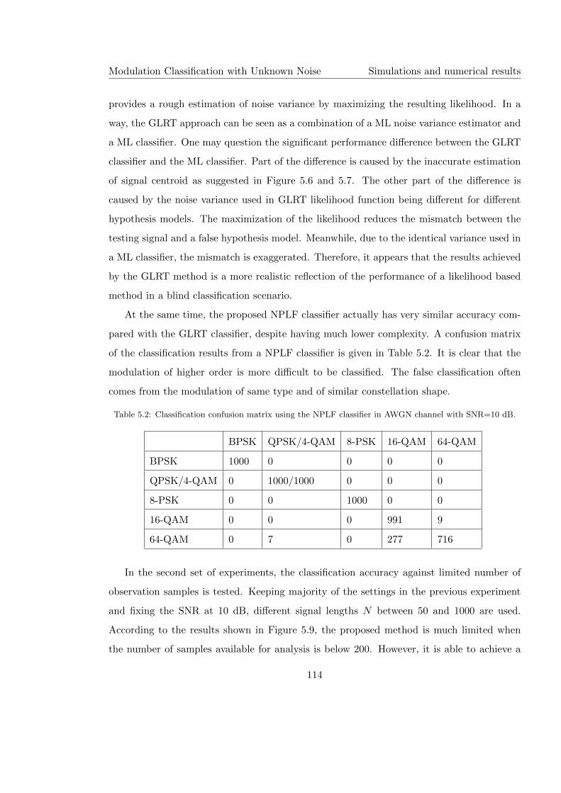
Modulation Classification with Unknown Noise Simulations and numerical results
provides a rough estimation of noise variance by maximizing the resulting likelihood. In a
way, the GLRT approach can be seen as a combination of a ML noise variance estimator and
a ML classifier. One may question the significant performance difference between the GLRT
classifier and the ML classifier. Part of the difference is caused by the inaccurate estimation
of signal centroid as suggested in Figure 5.6 and 5.7. The other part of the difference is
caused by the noise variance used in GLRT likelihood function being different for different
hypothesis models. The maximization of the likelihood reduces the mismatch between the
testing signal and a false hypothesis model. Meanwhile, due to the identical variance used in
a ML classifier, the mismatch is exaggerated. Therefore, it appears that the results achieved
by the GLRT method is a more realistic reflection of the performance of a likelihood based
method in a blind classification scenario.
At the same time, the proposed NPLF classifier actually has very similar accuracy com-
pared with the GLRT classifier, despite having much lower complexity. A confusion matrix
of the classification results from a NPLF classifier is given in Table 5.2. It is clear that the
modulation of higher order is more difficult to be classified. The false classification often
comes from the modulation of same type and of similar constellation shape.
Table 5.2: Classification confusion matrix using the NPLF classifier in AWGN channel with SNR=10 dB.
BPSK QPSK/4-QAM 8-PSK 16-QAM 64-QAM
BPSK 1000 0 0 0 0
QPSK/4-QAM 0 1000/1000 0 0 0
8-PSK 0 0 1000 0 0
16-QAM 0 0 0 991 9
64-QAM 0 7 0 277 716
In the second set of experiments, the classification accuracy against limited number of
observation samples is tested. Keeping majority of the settings in the previous experiment
and fixing the SNR at 10 dB, different signal lengths N between 50 and 1000 are used.
According to the results shown in Figure 5.9, the proposed method is much limited when
the number of samples available for analysis is below 200. However, it is able to achieve a
114
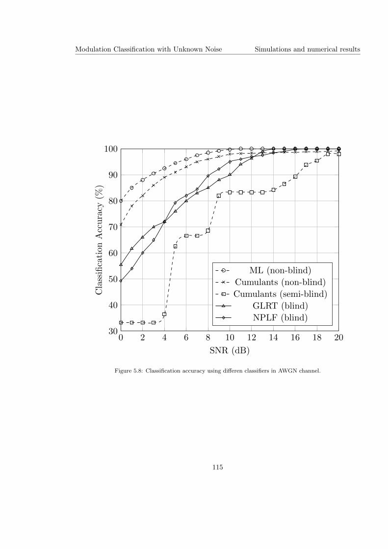
Modulation Classification with Unknown Noise Simulations and numerical results
0 2 4 6 8 10 12 14 16 18 2030
40
50
60
70
80
90
100
SNR (dB)
Cla
ssifi
cati
onA
ccu
racy
(%)
ML (non-blind)
Cumulants (non-blind)
Cumulants (semi-blind)
GLRT (blind)
NPLF (blind)
Figure 5.8: Classification accuracy using differen classifiers in AWGN channel.
115
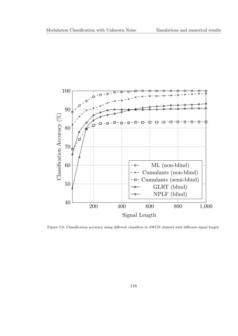
Modulation Classification with Unknown Noise Simulations and numerical results
200 400 600 800 1,00040
50
60
70
80
90
100
Signal Length
Cla
ssifi
cati
onA
ccu
racy
(%)
ML (non-blind)
Cumulants (non-blind)
Cumulants (semi-blind)
GLRT (blind)
NPLF (blind)
Figure 5.9: Classification accuracy using different classifiers in AWGN channel with different signal length.
116
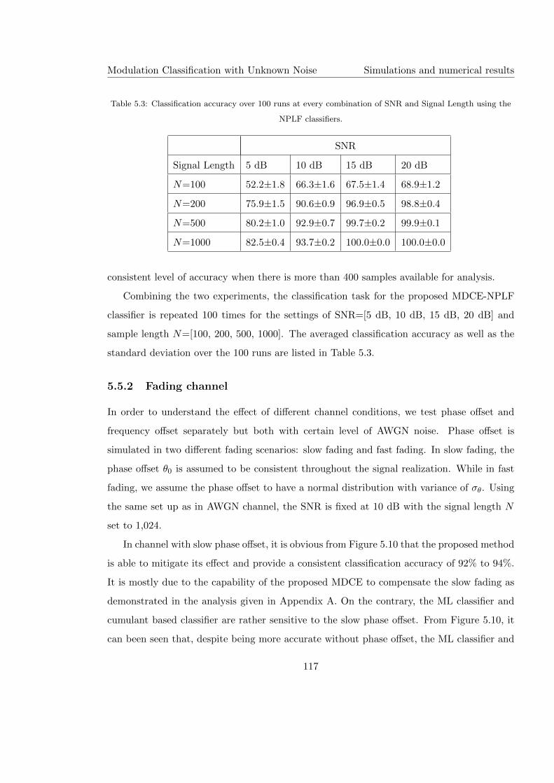
Modulation Classification with Unknown Noise Simulations and numerical results
Table 5.3: Classification accuracy over 100 runs at every combination of SNR and Signal Length using the
NPLF classifiers.
SNR
Signal Length 5 dB 10 dB 15 dB 20 dB
N=100 52.2±1.8 66.3±1.6 67.5±1.4 68.9±1.2
N=200 75.9±1.5 90.6±0.9 96.9±0.5 98.8±0.4
N=500 80.2±1.0 92.9±0.7 99.7±0.2 99.9±0.1
N=1000 82.5±0.4 93.7±0.2 100.0±0.0 100.0±0.0
consistent level of accuracy when there is more than 400 samples available for analysis.
Combining the two experiments, the classification task for the proposed MDCE-NPLF
classifier is repeated 100 times for the settings of SNR=[5 dB, 10 dB, 15 dB, 20 dB] and
sample length N=[100, 200, 500, 1000]. The averaged classification accuracy as well as the
standard deviation over the 100 runs are listed in Table 5.3.
5.5.2 Fading channel
In order to understand the effect of different channel conditions, we test phase offset and
frequency offset separately but both with certain level of AWGN noise. Phase offset is
simulated in two different fading scenarios: slow fading and fast fading. In slow fading, the
phase offset θ0 is assumed to be consistent throughout the signal realization. While in fast
fading, we assume the phase offset to have a normal distribution with variance of σθ. Using
the same set up as in AWGN channel, the SNR is fixed at 10 dB with the signal length N
set to 1,024.
In channel with slow phase offset, it is obvious from Figure 5.10 that the proposed method
is able to mitigate its effect and provide a consistent classification accuracy of 92% to 94%.
It is mostly due to the capability of the proposed MDCE to compensate the slow fading as
demonstrated in the analysis given in Appendix A. On the contrary, the ML classifier and
cumulant based classifier are rather sensitive to the slow phase offset. From Figure 5.10, it
can been seen that, despite being more accurate without phase offset, the ML classifier and
117
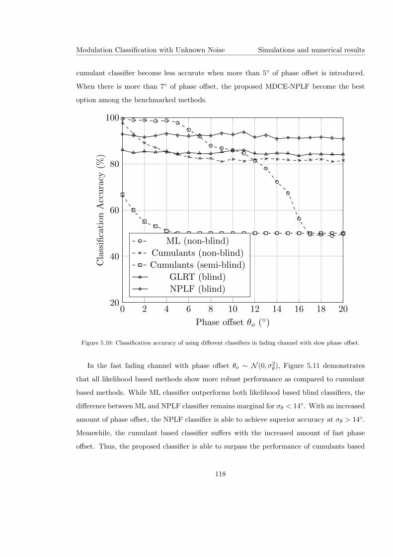
Modulation Classification with Unknown Noise Simulations and numerical results
cumulant classifier become less accurate when more than 5◦ of phase offset is introduced.
When there is more than 7◦ of phase offset, the proposed MDCE-NPLF become the best
option among the benchmarked methods.
0 2 4 6 8 10 12 14 16 18 2020
40
60
80
100
Phase offset θo (◦)
Cla
ssifi
cati
onA
ccu
racy
(%)
ML (non-blind)
Cumulants (non-blind)
Cumulants (semi-blind)
GLRT (blind)
NPLF (blind)
Figure 5.10: Classification accuracy of using different classifiers in fading channel with slow phase offset.
In the fast fading channel with phase offset θo ∼ N (0, σ2θ), Figure 5.11 demonstrates
that all likelihood based methods show more robust performance as compared to cumulant
based methods. While ML classifier outperforms both likelihood based blind classifiers, the
difference between ML and NPLF classifier remains marginal for σθ < 14◦. With an increased
amount of phase offset, the NPLF classifier is able to achieve superior accuracy at σθ > 14◦.
Meanwhile, the cumulant based classifier suffers with the increased amount of fast phase
offset. Thus, the proposed classifier is able to surpass the performance of cumulants based
118
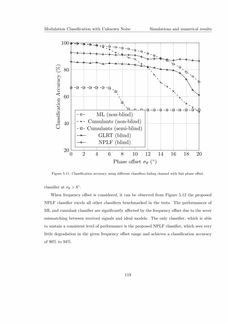
Modulation Classification with Unknown Noise Simulations and numerical results
0 2 4 6 8 10 12 14 16 18 2020
40
60
80
100
Phase offset σθ (◦)
Cla
ssifi
cati
onA
ccu
racy
(%)
ML (non-blind)
Cumulants (non-blind)
Cumulants (semi-blind)
GLRT (blind)
NPLF (blind)
Figure 5.11: Classification accuracy using different classifiers fading channel with fast phase offset.
classifier at σθ > 8◦.
When frequency offset is considered, it can be observed from Figure 5.12 the proposed
NPLF classifier excels all other classifiers benchmarked in the tests. The performances of
ML and cumulant classifier are significantly affected by the frequency offset due to the sever
mismatching between received signals and ideal models. The only classifier, which is able
to sustain a consistent level of performance is the proposed NPLF classifier, which sees very
little degradation in the given frequency offset range and achieves a classification accuracy
of 90% to 94%.
119

Modulation Classification with Unknown Noise Simulations and numerical results
0.2 0.4 0.6 0.8 1 1.2 1.4 1.6 1.8 2
·10−4
0
20
40
60
80
100
Frequency offset
Cla
ssifi
cati
onA
ccu
racy
(%)
ML (non-blind)
Cumulants (non-blind)
Cumulants (semi-blind)
GLRT (blind)
NPLF (blind)
Figure 5.12: Classification accuracy using different classifiers in fading channel with frequency offset.
120
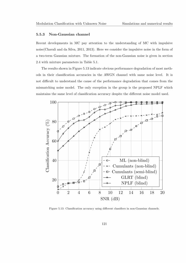
Modulation Classification with Unknown Noise Simulations and numerical results
5.5.3 Non-Gaussian channel
Recent developments in MC pay attention to the understanding of MC with impulsive
noise(Chavali and da Silva, 2011, 2013). Here we consider the impulsive noise in the form of
a two-term Gaussian mixture. The formation of the non-Gaussian noise is given in section
2.4 with mixture parameters in Table 5.1.
The results shown in Figure 5.13 indicate obvious performance degradation of most meth-
ods in their classification accuracies in the AWGN channel with same noise level. It is
not difficult to understand the cause of the performance degradation that comes from the
mismatching noise model. The only exception in the group is the proposed NPLF which
maintains the same level of classification accuracy despite the different noise model used.
0 2 4 6 8 10 12 14 16 18 20
20
40
60
80
100
SNR (dB)
Cla
ssifi
cati
onA
ccu
racy
(%)
ML (non-blind)
Cumulants (non-blind)
Cumulants (semi-blind)
GLRT (blind)
NPLF (blind)
Figure 5.13: Classification accuracy using different classifiers in non-Gaussian channels.
121

Modulation Classification with Unknown Noise Simulations and numerical results
Table 5.4: Number of operators needed for different classifiers.
Classifier Exponential Logarithm Multiplication Addition Memory
ML NII∑i=1
Mi NI 5NII∑i=1
Mi 6NII∑i=1
Mi I
Cumulant 0 0 6KN 6KN KI
GLRT V NII∑i=1
Mi V NI 5V NII∑i=1
Mi 6V NII∑i=1
Mi 2I
NPLF
(This research)
0 0 0 4NII∑i=1
Mi I
5.5.4 Complexity
To evaluate the complexity of different classifiers, numbers of operations needed are calcu-
lated for each classifier and listed in Table 5.4. The calculation is based on a signal with N
number of samples being classified among I potential modulations. Mi denotes the alphabet
size of the ith modulation candidate. The number of testing point for noise variance used
in GLRT is defined by V . And number of training sample in the cumulant based method is
defined by K.
Among all the tested methods, the ML classifier is known to have a very high computa-
tional complexity due to the large number of exponential and logarithmic operations needed.
For a GLRT classifier, the complexity is dramatically increased because the log-likelihood
evaluation is effectively repeated V times. Cumulants based classifiers have lower complexity
compared ML and GLRT classifier. However, the reference values needed for KNN classifier
impose a high demand for memory. The classifier with lowest complexity is the proposed
NPLF classifier which uses only additions and does not require extra memory allocation for
reference values.
5.6 Summary
In this chapter, the combination of centroid estimation and non-parametric likelihood func-
tion for modulation classification is studied. Two different approach to the centroid estima-
122
Modulation Classification with Unknown Noise Simulations and numerical results
tion are discussed. The constellation segmentation estimator is developed for fast centroid
estimation for square M-QAM modulations with the assumption of symbol assignment at
the transmitter end being equal probable. The minimum distance centroid estimator, on
the other hand, is much more versatile, which is able to both M-PSK and M-QAM mod-
ulations. The non-parametric likelihood function is proposed to realize likelihood function
without knowing either the noise model or the noise power. The numerical results show that
the combination of MDCE and NPLF is able to achieve good classification accuracy in the
AWGN channel. Moreover, the classifier shows stronger robustness in fading channel and
non-Gaussian channels. Last but not least, the computational complexity of the NPLF is
much lower compared with some of the existing methods.
123
Chapter 6
Blind Modulation Classification for
MIMO systems
6.1 Introduction
While majority of modulation classification algorithms have been dedicated to Single-input
Single-output (SISO) systems (Azzouz and Nandi, 1996b; Nandi and Azzouz, 1998; Azzouz
and Nandi, 1996a; Swami and Sadler, 2000; Dobre et al., 2007; Punchihewa et al., 2010;
Amuru and da Silva, 2012; Zhu et al., 2013b), blind modulation classification for multiple-
input multiple-output systems has become an attractive novelty. MIMO systems with asso-
ciated techniques such as Spatial Multiplexing (SM) and Space-time Coding (STC) provides
benefits including array gain and spatial gain for improved spectrum efficiency and link relia-
bility. Some recent publications address the issue of BMC for MIMO systems. Choqueuse et
al. developed the average likelihood ratio test classifier for MC with perfect channel knowl-
edge (Choqueuse et al., 2009). In the same paper, they proposed to use ICA with phase
correction for channel matrix estimation in order to achieve BMC. The ICA estimator is
endorsed by the following publications but accompanied with different classifiers (Muhlhaus
et al., 2013; Kanterakis and Su, 2013). Mhlhaus et al. proposed high order cumulants based
likelihood ratio test classifier for low complexity BMC (Muhlhaus et al., 2013). Kanterakis
124
Blind Modulation Classification for MIMO systems Signal model in MIMO systems
and Su suggest complexity reduction to the ALRT classifier by treating ICA recovered sig-
nal components at different transmitting antennas as individual processes (Kanterakis and
Su, 2013). Most ICA estimation aided classifier achieves very high classification accuracy.
However, the aforementioned methods require the perfect knowledge of noise variance. In
addition, the ICA estimation imposes the requirement that the number of receiving antennas
must exceed the number of transmitting antennas. Hassan et al. proposed a combination of
high order statistic and Artificial Neural Network (ANN) for MC. The method is successful in
addressing the issue of spatial correlation in MIMO systems (Hassan et al., 2012). However,
supervised training required by ANN makes it rather demanding as a blind classifier.
In this research, we propose a more practical BMC solution with both unknown channel
matrix and unknown noise variance. There is no existing BMC algorithms for such scenario
to our knowledge. Most state-of-the art channel estimation for MIMO systems depend on pi-
lot symbols for data aided estimation which is not suitable for BMC. Therefore, expectation
maximization is adopted for non-data aided blind channel estimation. The EM algorithm
approaches the channel estimate through an iterative process of maximizing the expected
likelihood. Compared to the ICA estimator, the EM estimator provides the additional esti-
mation of noise variance while not needing the phase correction for the channel matrix. The
resulting estimate is used for the maximum likelihood classifier for decision making.
6.2 Signal model in MIMO systems
Have defined signal models in different channels, we extend the definition to MIMO sys-
tems where multiple transmitters and receivers are considered to formulate multiple prop-
agation paths. The MIMO system is composed of Nt transmitting antennas and Nr re-
ceiving antennas. A Rayleigh fading channel with time invariant path gains is considered.
The resulting channel matrix H is given by a Nr × Nt complex matrix with the element
hj,i representing the path gain between ith transmitting antenna and jth receiving an-
tenna. Assuming perfect synchronization, the nth received MIMO-SM signal sample vector
125
Blind Modulation Classification for MIMO systems EM channel estimation
rn = [rn(1), rn(2), ..., rn(Nr)]T in a total observation of N samples is expressed as
rn = Hsn + ωn (6.1)
where sn = [sn(1), sn(2), ..., sn(Nt)]T is the nth transmitted signal symbol vector and ωn =
[ωn(1), ωn(2), ..., ωn(Nr)]T is the additive noise observed at the nth signal sample. The
transmitted symbol vector is assumed to be independent and identically distributed with each
symbol assigned from the modulation alphabet with equal probability. The additive noise is
assumed to be white Gaussian with zero mean and variance σ2 which gives ωn ∈ N (0, σ2INr),
where INr is the identity matrix of size Nr ×Nr.
6.3 EM channel estimation
To evaluate likelihood for the ML classifier, the complex channel matrix H and noise vari-
ance σ2 must be estimated beforehand. Since the modulation is unknown to the receiver,
many data-aided approaches using pilot symbols are not suitable. Expectation maximiza-
tion has been employed for joint channel estimation through an iterative implementation of
maximum likelihood estimation(Wautelet et al., 2007; Das and Rao, 2012). In MIMO sys-
tems, we consider the received signal R = [r1, r2...rN ] as the observed data. Meanwhile, the
membership Z of the observed samples is considered as the latent variables. Z is a M ×Nmatrix with the (m,n)th element being the membership of the nth signal sample rn, given
the transmitted symbol vector Sm. The possible transmitted symbol set S = [S1, S2...SM ]
gathers all the combinations of transmitted symbols from Nt number of antennas. Given a
modulation with L number of states, there exist M = LNt number of transmitted symbol
vectors and a transmitted symbol set of size Nt × LNt . With Θ = {H,σ2} representing the
channel parameters, the complete likelihood is given by
q(R,S|Θ) =
∫S
p(S|R,Θ) log(p(R|S,Θ)p(S|Θ))dS (6.2)
where p(R|S,Θ) is the probability of the received signal been observed given transmitted
symbols vector S and channel parameter Θ. Since the additive noise is assume to have a
126

Blind Modulation Classification for MIMO systems EM channel estimation
complex Gaussian distribution. p(R|S,Θ) can be calculated as
p(R|S,Θ) =
N∏n=1
1
(πσ2)Nrexp(−‖rn −Hsn‖
2F
2σ2). (6.3)
Meanwhile, p(S|R,Θ) represents the probability of S being transmitted given the ob-
served signal R and the channel parameter Θ, also know as the posteriori probability of S.
In (Wautelet et al., 2007), this probability is acquired by a posteriori probability calculator
which is not presented. In this research, we replace the a posteriori probability with a soft
membership znm representing the likelihood of nth transmitted symbol vector being Sm with∑Mm=1 zmn = 1. Since the assignment of transmitted symbol is independent of the channel
parameter, p(S|Θ) is a constant 1/M when equal probability is assumed. The estimation of
Θ is achieved by iterative steps of expectation evaluation and maximization.
6.3.1 Evaluation step
The evaluation step (E-step) provides the expected log-likelihood under the current estimate
of Θt at tth iteration. The expectation is then subsequently maximized for the updated
estimation of Θ. From Equation (6.2) the expected value of the complete log-likelihood is
derived as
Q(R,S|Θt) = log
N∏n=1
M∏m=1
p(rn, Sm|Ht, σ2t )zmn
= −N∑n=1
M∑m=1
zmn
[Nr log(πσ2
t ) +‖rn −HtSm‖2F
σ2
](6.4)
where p(rn, Sm|Ht, σt) is the probability of the nth received signal vector being observed
given the current estimation of channel matrixHt and noise variance σ2t . ‖·‖2F is the Frobenius
norm. The soft membership zmn is evaluated using the following equation
zmn =p(rn|Sm,Θt)M∑m=1
p(rn|Sm,Θt)
=exp(−‖rn−HSm‖
2F
σ2 )
M∑m=1
exp(−‖rn−HSm‖2F
σ2 )
. (6.5)
127
Blind Modulation Classification for MIMO systems EM channel estimation
6.3.2 Maximization step
The update of the parameter estimation is achieved through the maximization of the current
expected log-likelihood (M-step). To derive the close form update function for the channel
matrix and noise variance, we first find the derivatives of Q(R,S|Θt) with respect to H and
σ2 separately. Given that
‖rn −HSm‖2F =
Nr∑j=1
∣∣∣∣∣rn(j)−Nt∑i=1
hj,iSm(i)
∣∣∣∣∣2
(6.6)
the derivative of Q(R,S|Θt) with respect to the individual element h(j, i) of the channel
matrix is given by
∂Q(R,S|Θt)
∂hj,i
= −N∑n=1
M∑m=1
zmn
Nt∑i=1
hj,i∗|Sm(i)|2 − rn(j)∗Sm(i)
σ2(6.7)
In the same way, the derivative of Q(R,S|Θt) with respect to the noise variance σ2 is found
as
∂Q(R,S|Θt)
∂σ2= −
N∑n=1
M∑m=1
zmn
(−Nr
σ2+‖rn −HSm‖2F
σ4
)(6.8)
When the derivatives are set to zero, the update functions of hj,i and σ2 can be derived
from Equation (6.7) and (6.8). However, it is obvious that different channel parameters
are coupled. To simplify the maximization process, the coupled channel parameters are
estimated in turns. The path gain hj,i is estimated with the rest of the channel matrix
known and represented with the lasted estimate for each path gain. The path gains are
updated in ascending order with respect to j and i. The resulting update function for hj,i is
given by
ht+1j,i
=
N∑n=1
M∑m=1
zmn
[rn(j)Sm(i)∗ − Sm(i)∗
Nt∑k=1,k 6=i
h′k,iSm(k)
]N∑n=1
M∑m=1
zmn|Sm(i)|2(6.9)
128
Blind Modulation Classification for MIMO systems Maximum likelihood classifier
where h′k,i is the lasted estimate of path gain hk,i. At tth iteration, h′k,i = htk,i if it has not
been updated or h′k,i = ht+1k,i if it has been updated. After the channel matrix is completely
updated, Ht+1 is used to acquire the noise variance estimation.
σ2t+1 =
N∑n=1
M∑m=1
zmnNr∑j=1
∣∣∣∣rn(j)−Nt∑i=1
ht+1j,i Sm(i)
∣∣∣∣2Nr
N∑n=1
M∑m=1
zmn
(6.10)
The EM algorithm with such maximization process is known as expectation conditional
maximization. ECM shares the convergence property of EM (Meng and Rubin, 1993) and
can be constructed to converge at similar rate as the EM algorithm (Sexton, 2000). The
ECM joint estimation of channel parameters has previously been successfully applied in BMC
for SISO systems (Chavali and da Silva, 2011; Soltanmohammadi and Naraghi-Pour, 2013;
Chavali and da Silva, 2013).
6.3.3 Termination
The final estimation of channel matrix H and noise variance σ2 is achieve when the iterative
process is terminated by one of two conditions. The first condition terminates the process
when the estimation reaches convergence. The condition is represented numerically with the
different between the expected likelihoods of the current iteration and the previous iteration
along with a predefined threshold. In the second condition, termination is triggered when
the predefined number of iterations has been reached.
6.4 Maximum likelihood classifier
For classification likelihood evaluation, the average likelihood ratio test approach is adopted
(Choqueuse et al., 2009). The average likelihood function is given by
L(R|Θ) =N∏n=1
1
M
M∑m=1
1
(πσ2)Nrexp(−‖rn −HSm‖
2F
2σ2) (6.11)
129
Blind Modulation Classification for MIMO systems Simulation and numerical results
with the corresponding log-likelihood function derived as
logL(R|Θ) =−NNt log(M)−NNrlog(πσ2)+
N∑n=1
log
(M∑m=1
1
(πσ2)Nrexp(−‖rn −HSm‖
2F
2σ2)
)(6.12)
In the case of BMC, the channel matrix and noise variance estimated by EM is used to sub-
stitute the known values in the ALRT likelihood evaluation for each modulation hypothesis.
The likelihood evaluation of modulation candidate M is given by
logL(R|SMΘM) = −NNt log(M)−NNrlog(πσ2M)
+
N∑n=1
log
M∑m=1
1(πσ2M)Nr exp(−
∥∥∥rn − HMSMm ∥∥∥2
F
2σ2M
)
(6.13)
where SM is the transmitted symbol set defined by modulation M and ΘM is the channel
estimation for the same modulation candidate.
The resulting classification decision M is found by comparing the likelihood evaluated
from different modulation candidates. The modulation candidateM in the candidate pool M
which provides the highest likelihood with the observed data is assigned as the classification
decision.
M = argmaxM∈M
(logL(R|SM,ΘM)) (6.14)
6.5 Simulation and numerical results
To validate the proposed BMC algorithm, MIMO systems in Rayleigh fading channel with
AWGN noise is simulated for BMC. Three popular digital modulations are included in the
modulation candidate pool M={BPSK,QPSK,16-QAM}. Other digital modulations can be
classified in the same procedure with very little modification. In the simulation, two sets of
experiments are set up to investigate the classifier performance under different noise levels
and with different observation length. The specifications of the simulations are summarized
in Table 6.1.
130
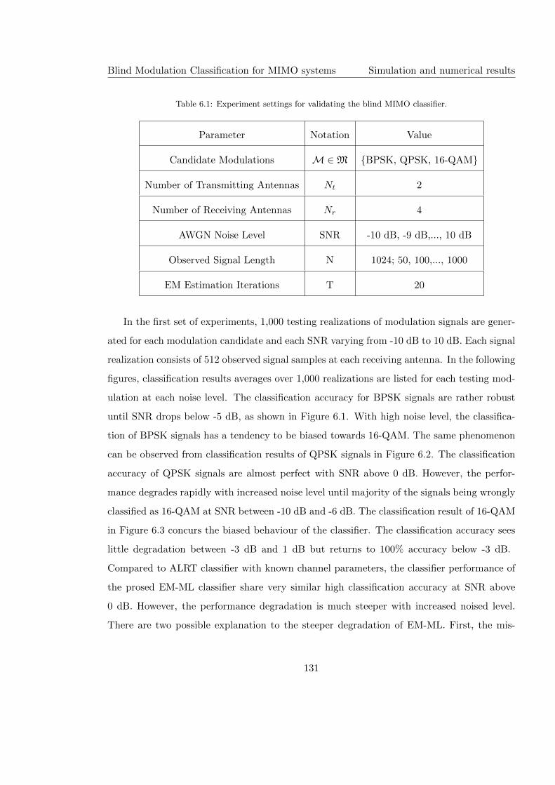
Blind Modulation Classification for MIMO systems Simulation and numerical results
Table 6.1: Experiment settings for validating the blind MIMO classifier.
Parameter Notation Value
Candidate Modulations M∈M {BPSK, QPSK, 16-QAM}
Number of Transmitting Antennas Nt 2
Number of Receiving Antennas Nr 4
AWGN Noise Level SNR -10 dB, -9 dB,..., 10 dB
Observed Signal Length N 1024; 50, 100,..., 1000
EM Estimation Iterations T 20
In the first set of experiments, 1,000 testing realizations of modulation signals are gener-
ated for each modulation candidate and each SNR varying from -10 dB to 10 dB. Each signal
realization consists of 512 observed signal samples at each receiving antenna. In the following
figures, classification results averages over 1,000 realizations are listed for each testing mod-
ulation at each noise level. The classification accuracy for BPSK signals are rather robust
until SNR drops below -5 dB, as shown in Figure 6.1. With high noise level, the classifica-
tion of BPSK signals has a tendency to be biased towards 16-QAM. The same phenomenon
can be observed from classification results of QPSK signals in Figure 6.2. The classification
accuracy of QPSK signals are almost perfect with SNR above 0 dB. However, the perfor-
mance degrades rapidly with increased noise level until majority of the signals being wrongly
classified as 16-QAM at SNR between -10 dB and -6 dB. The classification result of 16-QAM
in Figure 6.3 concurs the biased behaviour of the classifier. The classification accuracy sees
little degradation between -3 dB and 1 dB but returns to 100% accuracy below -3 dB.
Compared to ALRT classifier with known channel parameters, the classifier performance of
the prosed EM-ML classifier share very similar high classification accuracy at SNR above
0 dB. However, the performance degradation is much steeper with increased noised level.
There are two possible explanation to the steeper degradation of EM-ML. First, the mis-
131
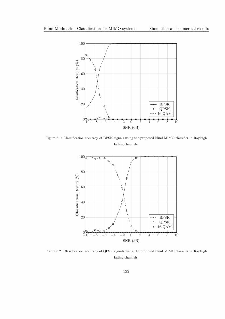
Blind Modulation Classification for MIMO systems Simulation and numerical results
−10 −8 −6 −4 −2 0 2 4 6 8 100
20
40
60
80
100
SNR (dB)
Cla
ssifi
cati
onR
esu
lts
(%)
BPSKQPSK
16-QAM
Figure 6.1: Classification accuracy of BPSK signals using the proposed blind MIMO classifier in Rayleigh
fading channels.
−10 −8 −6 −4 −2 0 2 4 6 8 100
20
40
60
80
100
SNR (dB)
Cla
ssifi
cati
onR
esu
lts
(%)
BPSKQPSK
16-QAM
Figure 6.2: Classification accuracy of QPSK signals using the proposed blind MIMO classifier in Rayleigh
fading channels.
132
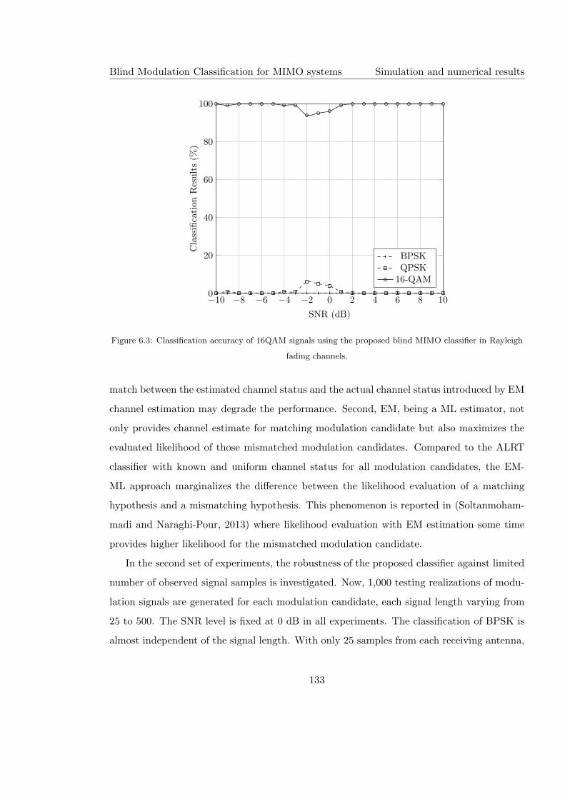
Blind Modulation Classification for MIMO systems Simulation and numerical results
−10 −8 −6 −4 −2 0 2 4 6 8 100
20
40
60
80
100
SNR (dB)
Cla
ssifi
cati
onR
esu
lts
(%)
BPSKQPSK
16-QAM
Figure 6.3: Classification accuracy of 16QAM signals using the proposed blind MIMO classifier in Rayleigh
fading channels.
match between the estimated channel status and the actual channel status introduced by EM
channel estimation may degrade the performance. Second, EM, being a ML estimator, not
only provides channel estimate for matching modulation candidate but also maximizes the
evaluated likelihood of those mismatched modulation candidates. Compared to the ALRT
classifier with known and uniform channel status for all modulation candidates, the EM-
ML approach marginalizes the difference between the likelihood evaluation of a matching
hypothesis and a mismatching hypothesis. This phenomenon is reported in (Soltanmoham-
madi and Naraghi-Pour, 2013) where likelihood evaluation with EM estimation some time
provides higher likelihood for the mismatched modulation candidate.
In the second set of experiments, the robustness of the proposed classifier against limited
number of observed signal samples is investigated. Now, 1,000 testing realizations of modu-
lation signals are generated for each modulation candidate, each signal length varying from
25 to 500. The SNR level is fixed at 0 dB in all experiments. The classification of BPSK is
almost independent of the signal length. With only 25 samples from each receiving antenna,
133
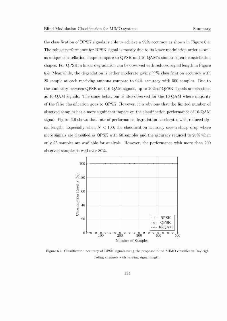
Blind Modulation Classification for MIMO systems Summary
the classification of BPSK signals is able to achieve a 99% accuracy as shown in Figure 6.4.
The robust performance for BPSK signal is mostly due to its lower modulation order as well
as unique constellation shape compare to QPSK and 16-QAM’s similar square constellation
shapes. For QPSK, a linear degradation can be observed with reduced signal length in Figure
6.5. Meanwhile, the degradation is rather moderate giving 77% classification accuracy with
25 sample at each receiving antenna compare to 94% accuracy with 500 samples. Due to
the similarity between QPSK and 16-QAM signals, up to 20% of QPSK signals are classified
as 16-QAM signals. The same behaviour is also observed for the 16-QAM where majority
of the false classification goes to QPSK. However, it is obvious that the limited number of
observed samples has a more significant impact on the classification performance of 16-QAM
signal. Figure 6.6 shows that rate of performance degradation accelerates with reduced sig-
nal length. Especially when N < 100, the classification accuracy sees a sharp drop where
more signals are classified as QPSK with 50 samples and the accuracy reduced to 20% when
only 25 samples are available for analysis. However, the performance with more than 200
observed samples is well over 80%.
100 200 300 400 5000
20
40
60
80
100
Number of Samples
Cla
ssifi
cati
onR
esu
lts
(%)
BPSKQPSK
16-QAM
Figure 6.4: Classification accuracy of BPSK signals using the proposed blind MIMO classifier in Rayleigh
fading channels with varying signal length.
134
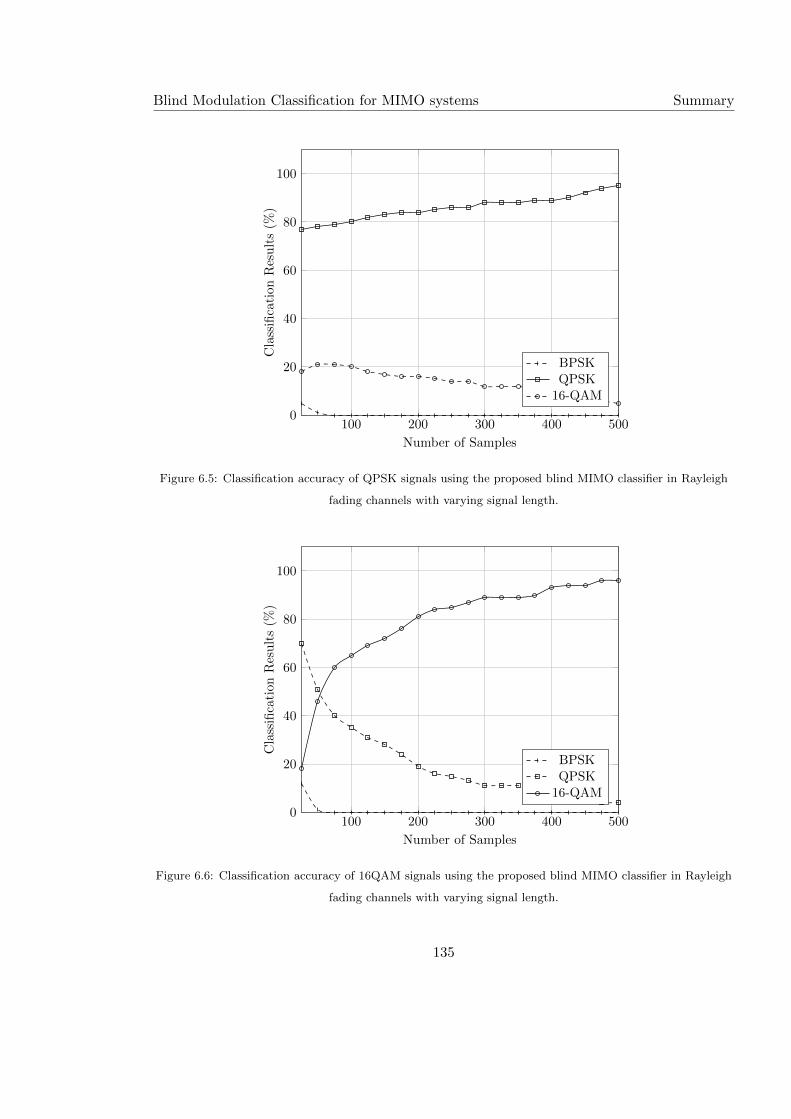
Blind Modulation Classification for MIMO systems Summary
100 200 300 400 5000
20
40
60
80
100
Number of Samples
Cla
ssifi
cati
onR
esu
lts
(%)
BPSKQPSK
16-QAM
Figure 6.5: Classification accuracy of QPSK signals using the proposed blind MIMO classifier in Rayleigh
fading channels with varying signal length.
100 200 300 400 5000
20
40
60
80
100
Number of Samples
Cla
ssifi
cati
onR
esu
lts
(%)
BPSKQPSK
16-QAM
Figure 6.6: Classification accuracy of 16QAM signals using the proposed blind MIMO classifier in Rayleigh
fading channels with varying signal length.
135
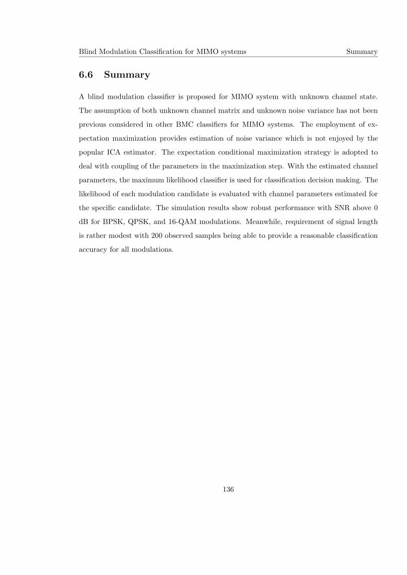
Blind Modulation Classification for MIMO systems Summary
6.6 Summary
A blind modulation classifier is proposed for MIMO system with unknown channel state.
The assumption of both unknown channel matrix and unknown noise variance has not been
previous considered in other BMC classifiers for MIMO systems. The employment of ex-
pectation maximization provides estimation of noise variance which is not enjoyed by the
popular ICA estimator. The expectation conditional maximization strategy is adopted to
deal with coupling of the parameters in the maximization step. With the estimated channel
parameters, the maximum likelihood classifier is used for classification decision making. The
likelihood of each modulation candidate is evaluated with channel parameters estimated for
the specific candidate. The simulation results show robust performance with SNR above 0
dB for BPSK, QPSK, and 16-QAM modulations. Meanwhile, requirement of signal length
is rather modest with 200 observed samples being able to provide a reasonable classification
accuracy for all modulations.
136
Chapter 7
Conclusions
In this chapter, we restate the purpose of the research and conclude what has been achieved
to further the field. In Chapter 1, it has been demonstrated that automatic modulation clas-
sification has an important role to play in both military and civilian applications. Although
a good modulation classification is expected to have high accuracy and robustness with low
computational complexity, the understanding we have developed through this research is
that there is no classifier that excels on all fronts. For example, maximum likelihood classifi-
cation provide optimal classification accuracy with the limitation of very high computational
complexity and high demand for channel knowledge. Moment and cumulant based classifiers
provide sub-optimal classification performance with lower complexity but suffers with signals
described by fewer samples. Distribution test based classifiers have improved robustness with
shorter signal but are more vulnerable against complex channels. With such an understand-
ing we set out to develop AMC algorithms that provide unique performance metrics that
excels in certain aspects or replaces certain existing methods with overall improvement.
The introduction of machine learning techniques in feature based AMC methods brings
four major benefits. First, the hierarchical decision making process is simplified with a sin-
gle step approach. Yet multi-stage classification strategy could still be accommodated for
performance optimization. Secondly, the determination of decision thresholds is automated
through training using a SVM classifier or become unnecessary in a KNN classifier. Thirdly,
the classification accuracy is improved over the traditional decision tree approach as demon-
137
Conclusions Summary
strated in the simulated experiments. Fourthly, the algorithm is simplified because of the
dimension reduction realized by feature selection and combination. However, the need for
training data is not often feasible. It is a major limitation of these supervised machine
learning techniques.
The optimized distribution sampling test classifier is an improvement over the KS test
classifier. While KS test is well established for measuring goodness of fit, in the case of
modulation classification, much information is underutilized to optimize the classification
performance. By establishing a set of optimized sampling location according to hypothesised
PDFs from modulation candidates, the ODST classifier is less vulnerable against outliers and
more efficient in using more information from the multiple locations on the spectrum. The
resulting benefit is higher classification accuracy as well as lower computational complex-
ity. The distribution based features inherent the same attributes from the ODST classifier
and extend to a wider set of signal distribution. The corresponding machine learning tech-
niques enables the consolidation of this big array of distribution based features to provide
more robust performance with the same level of efficiency. As non-blind classifiers, all of
the distribution test based classifiers are based on the assumption of perfection knowledge
of the transmission channel as well as the noise type and power. Predictably, these classi-
fiers are prone to performance degradation in the presence of channel estimation error and
mismatching channel mode.
The combination of centroid estimation and non-parametric likelihood function is an
unique approach to the modulation classification problem. It resembles the mechanism of
a likelihood based classifier. However it is not strictly likelihood that the NPLF is measur-
ing. In essence, it is estimating the cumulative probability of the received signal in a region
that is defined by the signal centroid and a normalized radius. Both factors jointly create a
total region of equal area for different candidate modulations. The resulting classifier does
not require a known noise model neither does it need the knowledge of noise power. The
performance is inferior compared to some of the non-blind classifiers with perfect channel
knowledge. However, when a GMM modelled impulsive noise is considered non-blind clas-
sifiers suffers greatly because of mismatching noise model. In the meantime, the NPLF
138
Conclusions Summary
classifier is able to sustain a consistent level of classification accuracy regardless of the type
of noise. That is without mentioning the significantly lower computational complexity. In
addition, the centroid estimation process is able to estimate the carrier phase offset and
achieves compensation in combination with the NPLF.
The extension of modulation classification to MIMO systems is very timely, considering
its wide application in 3G, 4G, and, predictably 5G cellular standards. In this research we
build on the likelihood based classifier for MIMO systems and reduce the amount of the
channel state information that is needed for the classifier. The EM process is developed for
the joint estimations of channel matrix and noise power. The resulting estimation enables the
likelihood evaluation based on a likelihood function that is adapted for the MIMO systems.
As the assumption of unknown noise power has yet been considered by other research, the
conclusion drawn from the simulated experiments is that the EM and ML combination
achieve good classification accuracy for BPSK, QPSK and 16-QAM modulations. Perfect
classification is observed when the SNR is above 0 dB in most cases. The demanded signal
length to achieve this performance is no more than for SISO systems. Due to the complexity
of MIMO systems, the likelihood evaluation is computationally much more expensive. In
fact, the complexity grows exponentially with the increasing modulation order as well as
number of transmitters.
In summary, our work has filled the void in the spectrum of existing methods with
low complexity classifiers of little compromise on classification accuracy. Novel classification
strategies have also been developed to solve modulation classification problems in more prac-
tical scenarios. As of now, much attention of modulation classifier development has shifted
towards MIMO systems. As stated above, computational complexity reduction is still a chal-
lenging task for MIMO systems, especially for higher order modulations and systems with
higher number of transmitter. It would be very interesting to adapt some of the SISO modu-
lation classifiers for the MIMO systems as only likelihood based classier has been considered
at the moment. While briefly touched upon in our experiments and discussions, the issues
of frequency offset is still not effectively solved by most of the current classifiers. To create
a classifier, especially a blind classifier, which is indeed practical in a real world situation,
139

Conclusions Summary
the ability to compensate frequency offset is extremely valuable and much desired.
140
Bibliography
Akay, M. F. Support Vector Machines Combined with Feature Selection for Breast Cancer
Diagnosis. Expert Systems with Applications, 36(2):3240–3247, 2009.
Amuru, S. and da Silva, C. R. C. M. Cumulant-based channel estimation algorithm for mod-
ulation classification in frequency-selective fading channels. In Military Communications
Conference, pages 1 – 6, 2012.
Aslam, M. W., Zhu, Z., and Nandi, A. K. Robust QAM Classification Using Genetic Pro-
gramming and Fisher Criterion. In European Signal Processing Conference, pages 995–999,
2011.
Aslam, M. W., Zhu, Z., and Nandi, A. K. Automatic Modulation Classification Using
Combination of Genetic Programming and KNN. IEEE Transactions on Wireless Com-
munications, 11(8):2742–2750, 2012.
Azzouz, E. E. and Nandi, A. K. Automatic Identification of Digital Modulation Types.
Signal Processing, 47(1):55–69, 1995.
Azzouz, E. E. and Nandi, A. K. Automatic Modulation Recognition of Communication
Signals. Kluwer, Boston, MA, 1996a.
Azzouz, E. E. and Nandi, A. K. Procedure for Automatic Recognition of Analogue and
Digital Modulations. IEE Proceedings - Communications, 143(5):259–266, 1996b.
Bennett, W. R. Methods of solving noise problems. Proceedings of the IRE, 44:609–638,
1956.
141

Conclusions Summary
Chan, Y. T. and Gadbois, L. G. Identification of the Modulation Type of a Signal. Signal
Processing, 1(4):838–841, 1989.
Chavali, V. G. and da Silva, C. R. C. M. Maximum-Likelihood Classification of Digital
Amplitude-Phase Modulated Signals in Flat Fading Non-Gaussian Channels. IEEE Trans-
actions on Communications, 59(8):2051 – 2056, 2011.
Chavali, V. G. and da Silva, C. R. C. M. Classification of Digital Amplitude-Phase Modulated
Signals in Time-Correlated Non-Gaussian Channels. IEEE Transactions on Communica-
tions, 61(6):2408–2419, 2013.
Choqueuse, V., Azou, S., Yao, K., Collin, L., and Burel, G. Blind Modulation Recognition
for MIMO Systems. Military Technical Academy Review, XIX(2):183–196, 2009.
Conover, W. Practical Nonparametric Statistics. Wiley, 1980.
Dan, W., Gu, X., and Qing, G. A New Scheme of Automatic Modulation Classification Using
Wavelet and WSVM. In Asia Pacific Conference on Mobile Technology, Applications and
Systems, pages 1–5. IEEE, 2005.
Das, A. and Rao, B. D. SNR and Noise Variance Estimation for MIMO Systems. IEEE
Transactions on Signal Processing, 60(8):3929–3941, 2012.
Dobre, O. A., Abdi, A., and Bar-Ness, Y. Survey of automatic modulation classification
techniques: classical approaches and new trends. IET Communications, 1(2):137–156,
2007.
Espejo, P. G., Ventura, S., and Herrera, F. A Survey on the Application of Genetic Pro-
gramming to Classification. IEEE Transactions on Systems, Man, and Cybernetics, Part
C (Applications and Reviews), 40(2):121–144, 2010.
Fabrizi, P. M., Lopes, L. B., and Lockhart, G. B. Receiver Recognition of Analogue Mod-
ulation Types. In IERE Conference on Radio Receiver and Associated Systems, pages
135–140, 1986.
142
Conclusions Summary
Fasano, G. and Franceschini, A. A Multidimensional Version of the Kolmogorov-Smirnov
Test. Monthly Notices of the Royal Astronomical Scoeity, 225:155–170, 1987.
Fisher, R. A. On the Mathematical Foundations of Theoretical Statistics. Philosophical
Transactions of the Royal Society A: Mathematical, Physical and Engineering Sciences,
222:309–368, 1922.
Gallager, R. G. Principles of Digital Communication. Cambridge University Press, 2008.
Gao, F., Cui, T., Nallanathan, A., and Tellambura, C. Maximum Likelihood Detection
for Differential Unitary Space-Time Modulation with Carrier Frequency Offset. IEEE
Transactions on Communications, 56(11):1881–1891, 2008.
Gardner, W. A. and Spooner, C. M. Signal interception: performance advantages of cyclic-
feature detectors. IEEE Transactions on Communications, 40(1):149–159, 1992.
Goldsmith, A. Wireless communications. Cambridge University Press, 2005.
Goldsmith, A. J. and Chua, S.-G. Adaptive Coded Modulation for Fading Channels. IEEE
Transactions on Communications, 46(5):595–602, 1998.
Gunn, S. R. Support Vector Machines for Classification and Regression. Technical Report 2,
1998.
Guo, H. and Nandi, A. K. Breast cancer diagnosis using genetic programming generated
feature. In Machine Learning for Signal Processing, IEEE Workshop on (MLSP), pages
215–220, 2006.
Hameed, F., Dobre, O. A., and Popescu, D. On the Likelihood-based Approach to Modu-
lation Classification. IEEE Transactions on Wireless Communications, 8(12):5884–5892,
2009.
Hassan, K., Dayoub, I., Hamouda, W., Nzeza, C. N., and Berbineau, M. Blind Digital
Modulation Identification for Spatially-Correlated MIMO Systems. IEEE Transactions
on Wireless Communications, 11(2):683–693, 2012.
143
Conclusions Summary
Hero, A. O. and Hadinejad-Mahram, H. Digital Modulation Classification Using Power Mo-
ment Matrices. In International Conference on Acoustics, Speech, and Signal Processing,
pages 3285–3288, 1998.
Hipp, J. E. Modulation Classification Based on Statistical Moments. In Military Communi-
cations Conference, pages 20.2.1 – 20.2.6, 1986.
Hong, L. and Ho, K. C. BPSK and QPSK Modulation Classification with Unknown Signal
Level. In Military Communications Conference, pages 976–980, 2000.
Hosmer, D. W. and Lemeshow, S. Applied Logistic Regression. Wiley, 2000.
Huang, C. Y. and Polydoros, A. Likelihood Methods for MPSK Modulation Classification.
IEEE Transactions on Communications, 43(2):1493–1504, 1995.
Jovanovic, S. D., Doroslovacki, M. I., and Dragosevic, M. V. Recognition of Low Modula-
tion Index AM Signals in Additive Gaussian Noise. In European Association for Signal
Processing V Conference, pages 1923–1926, 1990.
Kanterakis, E. and Su, W. Modulation Classification in MIMO Systems. In Military Com-
munications Conference, pages 35–39, 2013.
Kolmogorov, A. N. Sulla Determinazione Empirica di una Legge di Distribuzione. Giornale
dell’ Istituto Italiano degli Attuari, (4):83–91, 1933.
Koza, J. R. Genetic Programming: On the Programming of Computers by Means of Natural
Selection. The MIT Press, Cambridge, Massachusetts, 1992.
Leib, H. and Pasupathy, S. The phase of a vector perturbed by Gaussian noise and differ-
entially coherent receivers. IEEE Transactions on Information Theory, 34(6):1491–1501,
1988.
Liu, H. and Xu, G. Closed-form blind symbol estimation in digital communications. IEEE
Transactions on Signal Processing, 43(11), 1995.
144
Conclusions Summary
Massey, F. The Kolmogorov-Smirnov Test for Goodness of Fit. Journal of the American
Statistical Association, 46(253):68–78, 1951.
Meng, X.-L. and Rubin, D. B. Maximum Likelihood Estimation via the ECM Algorithm: a
General Framework. Biometrika, 80(2):267–278, 1993.
Middleton, D. Non-Gaussian Noise Models in Signal Processing for Telecommunications :
New Methods and Results for Class A and Class B Noise Models. IEEE Transactions on
Information Theory, 45(4):1129–1149, 1999.
Mobasseri, B. G. Digital modulation classification using constellation shape. Signal Process-
ing, 80(2):251–277, 2000.
Muhlhaus, M. S., Oner, M., Dobre, O. A., and Jondral, F. K. A Low Complexity Modulation
Classification Algorithm for MIMO Systems. IEEE Communications Letters, 17(10):1881–
1884, 2013.
Mustafa, H. and Doroslovacki, M. Digital Modulation Recognition Using Support Vector
Machine Classifier. Asilomar Conference on Signals, Systems and Computers, pages 2238–
2242, 2004.
Nandi, A. K. and Azzouz, E. E. Automatic Analogue Modulation Recognition. Signal
processing, 46:211–222, 1995.
Nandi, A. K. and Azzouz, E. E. Algorithms for automatic modulation recognition of com-
munication signals. IEEE Transactions on Communications, 46(4):431–436, 1998.
Panagiotou, P., Anastasopoulos, A., and Polydoros, A. Likelihood Ratio Tests for Modulation
Classification. In Military Communications Conference, pages 670–674, 2000.
Peacock, J. A. Two-dimensional Goodness-of-fit Testing Astronomy. Monthly Notices of the
Royal Astronomical Scoeity, 202:615–627, 1983.
Poisel, A. R. Introduction to Communication Electronic Warfare Systems. Artech House,
2008.
145
Conclusions Summary
Polat, K. and Gune, S. Breast Cancer Diagnosis Using Least Square Support Vector Machine.
Digital Signal Processing, 17(4):694–701, 2007.
Polydoros, A. and Kim, K. On the Detection and Classification of Quadrature Digital
Modulations in Broad-band Noise. IEEE Transactions on Communications, 38(8):1199–
1211, 1990.
Punchihewa, A., Zhang, Q., Dobre, O. A., Spooner, C. M., Rajan, S., and Inkol, R. On
the cyclostationarity of OFDM and single carrier linearly digitally modulated signals in
time dispersive channels: theoretical developments and application. IEEE Transactions
on Wireless Communications, 9(8):2588–2599, 2010.
Roberts, S. J. and Penny, W. D. Variational Bayes for Generalized Autoregressive Models.
IEEE Transactions on Signal Processing, 50(9):2245–2257, 2002.
Serpedin, E., Chevreuil, A., Giannakis, G., and Loubaton, P. Blind Channel and Carrier
Frequency Offset Estimation Using Periodic Modulation Precoders. IEEE Transactions
on Signal Processing, 48(8):2389–2405, 2000.
Sexton, J. ECM Algorithms That Converge at the Rate of EM. Biometrika, 87(3):651–662,
2000.
Shi, Q. and Karasawa, Y. Noncoherent Maximum Likelihood Classification of Quadrature
Amplitude Modulation Constellations: Simplification, Analysis, and Extension. IEEE
Transactions on Wireless Communications, 10(4):1312–1322, 2011.
Shi, Q. and Karasawa, Y. Automatic Modulation Identification Based on the Probability
Density Function of Signal Phase. IEEE Transactions on Communications, 60(4):1–5,
2012.
Sills, J. A. Maximum-likelihood Modulation Classification for PSK/QAM. In Military Com-
munications Conference, pages 217–220, 1999.
Silva, S. GPLAB - A Genetic Programming Toolbox for MATLAB. (http://goo.gl/zk1g2O),
2007.
146

Conclusions Summary
Smirnov, H. Sur les Ecarts de la Courbe de Distribution Empirique. Recueil Mathematique
(Matematiceskii Sbornik), (6):3–26, 1939.
Soliman, S. S. and Hsue, S.-Z. Signal Classification Using Statistical Moments. IEEE Trans-
actions on Communications, 40(5):908–916, 1992.
Soltanmohammadi, E. and Naraghi-Pour, M. Blind Modulation Classification over Fading
Channels Using Expectation-Maximization. IEEE Communications Letters, 17(9):1692–
1695, 2013.
Spooner, C. M. Classification of Co-channel Communication Signals Using Cyclic Cumulants.
In Conference Record of the Twenty-Ninth Asilomar Conference on Signals, Systems and
Computers, pages 531–536, 1996.
Swami, A. and Sadler, B. M. Hierarchical Digital Modulation Classification Using Cumulants.
IEEE Transactions on Communications, 48(3):416–429, 2000.
Theodoridis, S. Pattern Recognition. Academic Press, 4th edition, 2008.
Tomasoni, A. and Bellini, S. Efficient OFDM channel estimation via an information criterion.
IEEE Transactions on Wireless Communications, 12(3):1352–1362, 2012.
Urriza, P., Rebeiz, E., Pawelczak, P., and Cabric, D. Computationally Efficient Modu-
lation Level Classification Based on Probability Distribution Distance Functions. IEEE
Communications Letters, 15(5):476–478, 2011.
Vastola, K. S. Threshold detection in narrow-band non-Gaussian noise. IEEE Transactions
on Communications, 32(2):134–139, 1984.
Wang, F. and Wang, X. Fast and Robust Modulation Classification via Kolmogorov-Smirnov
Test. IEEE Transactions on Communications, 58(8):2324–2332, 2010.
Wautelet, X., Herzet, C., Dejonghe, A., Louveaux, J., and Vandendorpe, L. Comparison of
EM-Based Algorithms for MIMO Channel Estimation. IEEE Transactions on Communi-
cations, 55(1):216–226, 2007.
147
Conclusions Summary
Wei, W. and Mendel, J. M. Maximum-Likelihood Classification for Digital Amplitude-Phase
Modulations. IEEE Transactions on Communications, 48(2):189–193, 2000.
Wong, M. L. D. and Nandi, A. K. Automatic Digital Modulation Recognition Using Artificial
Neural Network and Genetic Algorithm. Signal Processing, 84(2):351–365, 2004.
Wong, M. L. D. and Nandi, A. K. Semi-blind Algorithms for Automatic Classification of
Digital Modulation Schemes. Digital Signal Processing, 18(2):209–227, 2008.
Wong, M. L. D., Ting, S. K., and Nandi, A. K. Naive Bayes classification of adaptive broad-
band wireless modulation schemes with higher order cumulants. International Conference
on Signal Processing and Communication Systems, (Ml):1–5, 2008.
Wu, H., Saquib, M., and Yun, Z. Cumulant Features for Communications via Multipath
Channels. IEEE Transactions on Wireless Communications, 7(8):3098–3105, 2008.
Wu, Z., Wang, X., Gao, Z., and Ren, G. Automatic Digital Modulation Recognition Based
on Support Vector Machines. In International Conference on Neural Networks and Brain,
volume 2, pages 1025–1028. IEEE, 2005.
Xu, J. L., Su, W., and Zhou, M. Likelihood-Ratio Approaches to Automatic Modulation
Classification. IEEE Transactions on Systems, Man, and Cybernetics, Part C (Applica-
tions and Reviews), 41(4):455–469, 2011.
Zarzoso, V. and Nandi, A. K. Blind separation of independent sources for virtually any source
probability density function. IEEE Transactions on Signal Processing, 47(9):2419–2432,
1999.
Zhu, Z. and Nandi, A. K. Blind Digital Modulation Classification using Minimum Dis-
tance Centroid Estimator and Non-parametric Likelihood Function. IEEE Transactions
on Wireless Communications, pages 1–12 (early access), 2014a.
Zhu, Z. and Nandi, A. K. Blind Modulation Classification for MIMO Systems using Expec-
tation Maximization. In Military Communications Conference, pages 1–6 (under review).
IEEE, 2014b.
148
Conclusions Summary
Zhu, Z., Aslam, M. W., and Nandi, A. K. Augmented Genetic Programming for Automatic
Digital Modulation Classification. In IEEE International Workshop on Machine Learning
for Signal Processing, pages 391–396, 2010.
Zhu, Z., Aslam, M. W., and Nandi, A. K. Support Vector Machine Assisted Genetic Pro-
gramming for MQAM Classification. In International Symposium on Signals, Circuits and
Systems, pages 1–6, 2011.
Zhu, Z., Aslam, M. W., and Nandi, A. K. Adapted Geometric Semantic Genetic Program-
ming for Diabetes and Breast Cancer Classification. In IEEE International Workshop on
Machine Learning for Signal Processing, pages 1–5, 2013a.
Zhu, Z., Nandi, A. K., and Aslam, M. W. Approximate Centroid Estimation with Constel-
lation Grid Segmentation for Blind M-QAM Classification. In Military Communications
Conference, number 1, pages 46–51, 2013b.
Zhu, Z., Nandi, A. K., and Aslam, M. W. Robustness Enhancement of Distribution Based Bi-
nary Discriminative Features for Modulation Classification. In IEEE International Work-
shop on Machine Learning for Signal Processing, pages 1–6, 2013c.
Zhu, Z., Aslam, M. W., and Nandi, A. K. Genetic Algorithm Optimized Distribution Sam-
pling Test for M-QAM Modulation Classification. Signal Processing, 94:264–277, 2014.
149

Appendix A: Minimum Distance
Centroid Estimation
The distance between a signal sample r(n) = αejθs(n) and an estimated centroid AmM =
aejφsmM can be written as
D(r(n),AmM) = ‖r(n)−AmM‖
=
√α2 ‖r(n)‖2 + a2
∥∥smM∥∥2 − 2α ‖s(n)‖ a∥∥smM∥∥ cos(θ − φ) (7.1)
Assuming a signal sample is assigned to its nearest centroid s(n) = smM, we replace the
expression for r(n) and AM with r(n) = αejθ and AmM = aejφ, where α = αs(n) and
a = asmM, for a more concise presentation.
Given that all signal symbol assignments are equiprobable, the expectation of signal-to-
centroid distance is given in equation (29).
E[DM(r, a, φ)] = (7.2)
N
M
∞∫0
φ+π/M∫φ−π/M
√x2 + a2 − 2ax cos(y − φ)fmag(x|α, σ)
M∑m=1
fphase(y|θ +mπ/M, σ)dydx
∂
∂φE[DM(r, φ)] = (7.3)
N
M
∞∫0
π/M∫−π/M
√x2 + a2 − 2ax cos(y)fmag(x|α, σ)
M∑m=1
∂
∂(y + φ)fphase(y + φ|θ +mπ/M, σ)dydx
150

Appendix A. Minimum Distance Centroid Estimation Summary
∂
∂aE[DM(r, a)] =
N
M
∞∫0
π/M∫−π/M
2a− 2x cos(y)
2√x2 + a2 − 2xa cos(y)
fmag(x|α, σ)M∑m=1
fphase(y + π/M |θ +mπ/M, σ)dydx
(7.4)
We take the derivative of E[DM(r, a, φ)] with respect of the centroid parameter phase φ
as in equation (30).
Given the signal phase distribution from a single symbol in AWGN channel (Bennett,
1956)
fphase(φ)
=e−α
2/2σ2
2π+α cos(φ)
2σ√
2π· [1 + erf(
α cos(φ)√2σ
)]e−α2
2σ2 sin2(θ), (7.5)
we simplify the distribution to its von Mises distribution approximation which converges to
equation (32) at high SNR (Leib and Pasupathy, 1988).
fphase(φ) =e(α2/σ2)cos(φ−µ)
2πI0(α2/σ2). (7.6)
The derivative of the distribution with respect to φ can be found as
∂
∂φfphase(φ) = − α2 sin(φ− µ)
σ22πI0(α2/σ2)e(α2/σ2) cos(φ−µ) (7.7)
which has the property that fphase′(α + φ|α, σ) = −f ′(α − φ|α, σ) and fphase
′(α|α, σ) = 0.
The two possible solutions for ∂∂φE[DM(r, a, φ)] can be found as φ = θ + mπ/M and
φ = θ+ (2m− 1)π/2M . It is not difficult to see that φ = θ+mπ/M provides the maximum
for E[DM(r, a, φ)] while φ = θ + (2m − 1)π/2M delivers the minimum. The term mπ/M
equals the phase difference between received signal centroids which introduces a relative shift
of carrier phase to the estimated carrier phase estimation. However, in modulation classifica-
tion, as long as the resulting centroids have a matching pattern with the true signal means,
the relative phase is of no concern. Therefore, the estimated centroid phase is accurate.
151

Appendix A. Minimum Distance Centroid Estimation Summary
Moreover, in a channel with phase offset, it is not difficult to see that the slow fading,
which adds a constant phase offset θo, results in a compensated of the shifted carrier phase
φ = θ + mπ/M + θo. In fast fading channel with θo ∼ N (0, σ2θ), the single signal phase
distribution is modified to
fphase(φ) =
µ+π∫µ−π
e(α2/σ2)cos(x−µ)
2πI0(α2/σ2)· 1
σθ√
2πe− (x−φ)2
2σ2θ dx (7.8)
with the derivative of the distribution with respect to φ
∂
∂φfphase(φ)
=
µ+π∫µ−π
(x− φ)
2√
2σ3θπ
3/2I0(α2/σ2)· e− (x−φ)
2σ2θ
+(α2/σ2)cos(x−µ)dx (7.9)
which leads to the same conclusion of φ = θ +mπ/M .
Now, let us consider the estimation of channel gain. The derivative of the distance
expectation with respect to centroid parameter magnitude is given in equation (31). The
magnitude PDF of a PSK modulated signal in AWGN channe is a Rice distribution
fmag(x) =x
σ2e(−(x2+α2)
2σ2 )I0(xα
σ2) (7.10)
where I0(·) is the modified Bessel function of the first kind of order zero. This distribution
is often approximated as a normal distribution when α/σ is big enough.
fmag(x) =1
σ√
2πe−
(x−α)2
2σ2 (7.11)
If the condition for the approximation can be met, a = α would be a solution of
∂∂aE[DM(r, a)] = 0. A more accurate approximation would be
fmag(x) =1
σ√
2πe−
(x−µ)2
2σ2 (7.12)
where µ = σ√
2/πL1/2(−α2/2σ2) is the mean of the Rice distribution. The resulting error
of channel gain estimation can be found as σ√
2/πL1/2(−α2/2σ2) − α, which converges to
zero when SNR→∞.
The analysis for QAM modulation is not given in this research. However, it can be easily
derived by considering it as a combination of components with the same magnitude which
can be treated similarly as PSK signals.
152
Appendix B: Iterative Minimum
Distance Estimator
With A represented in a complex form x+ jy, the sub-gradient at A = x+ jy is obtained as
∇D(x, y) =D(x+ ∆x, y)
∆x+ j
D(x, y + ∆y)
∆y. (7.13)
The update function for An = xn + jyn is expressed as
xn+1 + jyn+1 = xn + jyn − αM∇D(xn, yn) (7.14)
The iterative process starts with A0 = x0 + jy0 and should update the estimation for 20
iterations unless the termination condition is met that the sub-gradient is lower than the
defined threshold.
∇D(x, y) < ηD (7.15)
The values of parameter used in the centroid estimation is given in Table 7.1.
153

Appendix B. Iterative Minimum Distance Estimator Summary
Table 7.1: Parameters used in the minimum distance estimator
Parameters Notation Simulation Values
Staring point A0 = x0 + jy0 0.1 + 0.1j,
Update step αM {2E − 4, 2E − 4, 5E − 5}{2E − 4, 5E − 5, 1E − 5}
Sub-gradient step ∆x, ∆y 0.01
Update iterations 20
Termination threshold ηD 10
154
Appendix C: Non-parametric
Likelihood Function
For both PSK and QAM modulation, it is not difficult to derive that NM− = MM− and
NM0 = NM+ = MM0 . In order to satisfy E[LNPLF (r|HM0)] > E[LNPLF (r|HM−)], the
following inequality needs to be satisfied.
MM0
RM0∫0
x
σ2e−x
2/2σ2dx > MM−
RM−∫0
x
σ2e−x
2/2σ2dx (7.16)
Simplify the above inequality with cumulative probability function of a Rayleigh distribution
F (x) = 1− e−x2/2σ2.
MM0(1− e−R2M0/2σ
2
) > MM−(1− e−R2M−
/2σ2
) (7.17)
Replacing both test radius with equation (21) and considering all modulation cases, the
restriction for the reference radius can be written as
R0 > 2
√2 log(
1
2−√
2)σ ≈ 2.07σ. (7.18)
Limiting the SNR in the range between 0 dB to 20 dB, taking the maximum of σ equals to
α when SNR is 0 dB. The limit for reference radius can be given by R0 > 2.07α.
In the case when false hypothesis is a modulation of higher order, the likelihood function
needs to satisfy E[LNPLF (r|HM0)] > E[LNPLF (r|HM+)] and
MM0(1− e−R2M0/2σ
2
) > MM0(1− e−R2M+/2σ
2
). (7.19)
155

Appendix C. Non-parametric Likelihood Function Summary
It is not difficult to see that with RM0 > RM+ , according to equation (21), the condition is
always met and imposes no restriction on the test radius.
156