Int J Comput VisDOI 10.1007/s11263-013-0672-6

Automatic and Efficient Human Pose Estimation for SignLanguage Videos

James Charles · Tomas Pfister · Mark Everingham ·Andrew Zisserman

Received: 4 February 2013 / Accepted: 29 October 2013© Springer Science+Business Media New York 2013

Abstract We present a fully automatic arm and handtracker that detects joint positions over continuous sign lan-guage video sequences of more than an hour in length. Toachieve this, we make contributions in four areas: (i) we showthat the overlaid signer can be separated from the backgroundTV broadcast using co-segmentation over all frames witha layered model; (ii) we show that joint positions (shoul-ders, elbows, wrists) can be predicted per-frame using arandom forest regressor given only this segmentation anda colour model; (iii) we show that the random forest canbe trained from an existing semi-automatic, but computa-tionally expensive, tracker; and, (iv) introduce an evaluatorto assess whether the predicted joint positions are correctfor each frame. The method is applied to 20 signing footagevideos with changing background, challenging imaging con-ditions, and for different signers. Our framework outper-forms the state-of-the-art long term tracker by Buehler et al.

Electronic supplementary material The online version of thisarticle (doi:10.1007/s11263-013-0672-6) contains supplementarymaterial, which is available to authorized users.

Mark Everingham, who died in 2012, made a significant contributionto this work. For this reason he is included as a posthumous author.An appreciation of his life and work can be found in Zisserman et al.(2012).

J. Charles · M. EveringhamSchool of Computing, University of Leeds, Leeds, UKe-mail: j.charles@leeds.ac.uk

M. Everinghame-mail: m.everingham@leeds.ac.uk

T. Pfister (B) · A. ZissermanDepartment of Engineering Science, University of Oxford, Oxford, UKe-mail: tp@robots.ox.ac.uk

A. Zissermane-mail: az@robots.ox.ac.uk

(International Journal of Computer Vision 95:180–197,2011), does not require the manual annotation of that work,and, after automatic initialisation, performs tracking in real-time. We also achieve superior joint localisation results tothose obtained using the pose estimation method of Yang andRamanan (Proceedings of the IEEE conference on computervision and pattern recognition, 2011).

Keywords Sign language · Human pose estimation ·Co-segmentation · Random forest

1 Introduction

A number of recent papers have demonstrated that signscan be recognised automatically from signed TV broadcasts(where an overlaid signer describes the broadcast) using onlyweak and noisy supervision (Buehler et al. 2009; Cooperand Bowden 2009; Farhadi and Forsyth 2006). For example,by using the correlations between subtitles and signs bothBuehler et al. (2009) and Cooper and Bowden (2009) wereable to automatically extract sign-video pairs from TV broad-casts; these automatically extracted sign-video pairs couldthen be used as supervisory material to train a sign languageclassifier Buehler et al. (2010) to recognise signs in new mate-rial. However, current research in this area has been held backby the difficulty of obtaining a sufficient amount of trainingvideo with the arms and hands of the signer annotated. Thisis a great pity because there is a practically limitless supplyof such signed TV broadcasts.

The standard approach of Buehler et al. (2011) for track-ing arms and hands in sign language TV broadcasts requiresmanual labelling of 64 frames per video, which is aroundthree hours of manual user input per one hour of TV footage.In addition, the tracker (by detection) is based on expensive

123

Int J Comput Vis

Segmentation Colour Model Random Forest RegressorInput

Fig. 1 Arm and hand joint positions are predicted by first segmenting the signer using a layered foreground/background model, and then feedingthe segmentation together with a colour model into a random forest regressor

(a) (b)

(c) (d)

Fig. 2 Challenges for joint tracking. a Similar foreground and back-ground colours render the colour cue less informative; b motion blurremoves much of the edges of the arm; c a face in the backgroundrenders the face detector-based colour model initialisation difficult; dproximity of the two hands makes the assignment to left and right handambiguous

computational models and requires hundreds of secondscomputation time per frame. Furthermore, signed TV broad-casts are very challenging material to segment and determinehuman joint positions on for a number of reasons that include:self-occlusion of the signer, self-shadowing, motion blur dueto the speed of the signing, and, in particular, the changingbackground (since the signer is superimposed over a mov-ing video that frequently even contains other people, e.g. seeFigs. 1 and 2). These three factors have hindered the largescale application of this method.

In this paper we describe a method for tracking joint posi-tions (of arms and hands) without any manual annotation

and, once initialised, the system runs in real-time. The threekey ideas are (i) for signed video the signer can be segmentedautomatically using co-segmentation (Sect. 2), (ii) given thesegmentation, the joint positions can be predicted using a ran-dom forest, and (iii) the random forest can be trained usingBuehler et al.’s tracking output, with no manual annotation(Sect. 3). We show that the random forest trained in this man-ner generalises to new signers (Sect. 5). Figure 1 illustratesthe processing steps.

Each of the ideas has more general applicability: (i) theco-segmentation method can be easily generalised to othersimilarly laid out TV broadcasts, e.g. the majority of EUcountries broadcast their signed TV broadcasts in a formatsuitable for this method; (ii) joint positions can be predictedby a random forest regressor in general, once the person issegmented from the background [as in the Kinect line ofresearch Shotton et al. (2008)]; and (iii) the random foresttracker can be trained from existing tracked data with quitesome generalisation over clothing and body mass (Charles etal. 2013).

This paper is an extended version of our BMVC 2012paper Pfister et al. (2012). In addition to a more detailedexposition, we include here an extensive set of new experi-ments with a much larger dataset (20 TV broadcast videosinstead of 5), a pose evaluator (Sect. 4) that provides an indi-cation of whether the joint predictions are correct or not, anda comparison with the joint prediction method of (Yang andRamanan 2011).

1.1 Related work

1.1.1 Random forests

The innate versatility of random forests (RFs) (Amit andGeman 1997; Breiman 2001) makes them suitable for a vari-ety of machine learning tasks (Criminisi et al. 2012), such asclassification, regression and clustering. They are naturallymulti-class and contain a structure which lends itself to par-allelisation and multi-core implementations (Sharp 2008).Along with these properties, the ever increasing computing

123

Int J Comput Vis

power and training data over recent years has spurred theinterest in RFs and fern-based Ozuysal et al. (2010) meth-ods in computer vision literature. They have been applied to avariety of problems, including image classification (Bosch etal. 2007; Marée et al. 2005), object detection (Gall and Lem-pitsky 2009; Criminisi et al. 2011; Kontschieder et al. 2012),image/video segmentation tasks (Shotton et al. 2008; Yin etal. 2007; Geremia et al. 2011; Nowozin et al. 2011) and fea-ture extraction (Liu et al. 2012). RFs are also fast to resolveat inference time, therefore lending themselves to real-timeapplications of tracking (Lepetit and Torr 2006; Santner etal. 2010; Apostoloff and Zisserman 2007).

In particular, we are interested in the work on humanpose estimation where RFs have been used for head poseestimation (Fanelli et al. 2011) and detecting facial featurepoints (Fanelli et al. 2012; Dantone et al. 2012; Cootes et al.2012). Of special regard are the methods for inferring fullbody pose, where notable success has been achieved usingdepth imagery. By applying a classification forest, Shottonet al. (2011) were able to segment a 3D depth map of a personinto body parts and use the segmentation as a stepping stonefor computing body joint locations. A performance boostwas found by Girshick et al. (2011) using regression forestsand Hough voting. Further improvements in accuracy on thesame dataset were obtained by Taylor et al. (2012) usingan RF to form dense correspondences between depth imagepixels and a 3D body model surface, enabling the use of aone-shot optimisation procedure to infer pose. Recently Sunet al. (2012) have conditioned the RF on a global variable,such as torso orientation, to enhance performance.

The success of these full body pose estimation methodsdepends upon the use of depth imagery. Depth images arecolour and texture-invariant and make background subtrac-tion much easier. This substantially reduces the variabilityin human appearance. The remaining variability due to bodyshape, pose and camera angle is accounted for by trainingwith large quantities of data. In the same spirit, we proposean upper body pose estimation method that exploits the largequantities of training data available and the efficiency andaccuracy of RFs. However, our method does not depend upondepth imagery for success, but instead uses raw RGB imageswith only a partially known background.

1.1.2 Pose Estimation

There is a vast array of literature regarding human pose esti-mation due to a huge array of different applications reliant onanalysing people in images and video (Moeslund 2011). It iscommon to use pictorial structures (Felzenszwalb and Hut-tenlocher 2005; Ramanan 2006; Ramanan et al. 2007; Sivicet al. 2006) to model human pose due to low computationalcomplexity during inference. In more recent work, the focushas been on improving the appearance models used in pictor-

ial structures for modelling the individual body parts (Eichnerand Ferrari 2009; Eichner et al. 2012; Andriluka et al. 2012;Johnson and Everingham 2009; Sapp et al. 2010). Buildingupon the pictorial structure framework, Felzenszwalb et al.(2008, 2010) proposed deformable part based models. It hasbeen shown by Yang and Ramanan (2011) that a mixture ofdeformable parts can be used in a tree structured model toefficiently model human pose. This results in a very generaland powerful pose estimation framework which we compareto our method in Sect. 5.3.4. Sapp et al. (2011) model bodyjoints rather than limbs, and also track joints across frames,using a set of tree-structured sub-models. We have not yetexplored in our work the benefit of tracking the predictedjoints over time.

Previous work on pose estimation for sign language recog-nition (Cooper and Bowden 2007; Starner et al. 1998a;Farhadi et al. 2007; Buehler et al. 2011; Pfister et al. 2012) invideos has relied on accurate hand tracking where it is popularto use skin colour for hand detection, although other detectorsbased on sliding window classifiers using Haar-like imagefeatures (Kadir et al. 2004; Ong and Bowden 2004; Dreuwet al. 2012) have been used. Of particular relevance here isthe method of Buehler et al. (2011) which used a genera-tive model for both the foreground (signer) and background(the image area surrounding the signer). The foreground wasgenerated by rendering colour models of the limbs and torsoin back-to-front depth order (the “painter’s algorithm”) sothat occlusions were handled correctly. The computationalexpenses of evaluating all such renderings was reduced bysampling from a pictorial structure proposal distribution.

1.1.3 Co-segmentation

Co-segmentation methods (Rother et al. 2006; Hochbaumand Singh 2009; Joulin et al. 2010; Chai et al. 2011) con-sider sets of images where the appearance of foregroundand/or background share some similarities, and exploit thesesimilarities to obtain accurate foreground-background seg-mentations. Rother et al. (2006) originally introduced theproblem of co-segmenting image pairs. Their approach wasto minimise an energy function with an additional histogrammatching term that forces foreground histograms of imagesto be similar. Hochbaum and Singh (2009) modified the his-togram matching term to enable the use of max flow-basedalgorithms. More recently, Chai et al. (2011, 2012) proposedco-segmentation algorithms that work on each image cate-gory separately, and embed class-discriminative informationinto the co-segmentation process.

In our case our co-segmentation algorithm automaticallyseparates signers from any signed TV broadcast by buildinga layered model (Jojic and Frey 2001; Szeliski et al. 2000;Kumar et al. 2008). We use this layered model of the signer to

123

Int J Comput Vis

FG DBG SBG

Fig. 3 Generative layered model of each frame. The co-segmentationalgorithm separates the signer from any signed TV broadcast by buildinga layered model consisting of a foreground (FG), dynamic background(DBG) and static background (SBG)

provide a suitable input representation for the random forestregressor that is superior to using the raw input image itself.

1.1.4 Sign Language Recognition

Previous studies in sign language recognition rely on datagenerated by performers signing words under controlledconditions. Learning to recognise signs usually dependsupon obtaining ground truth data and the ability to trackthe signers’ head and hand positions (Vogler and Metaxas1998; Dreuw et al. 2006; Starner et al. 1998b). Heavy con-straints are typically imposed, such as wearing motion sen-sors (Chunli et al. 2002) or using a uniform backgroundand/or wearing coloured gloves. Generating a small amountof such data with ground truth is both labour-intensive andexpensive. It is possible to learn signs with small quantitiesof labelled data (Kadir et al. 2004; Bowden et al. 2004), butto increase the vocabulary of recognisable signs from 100sof words to 1,000s of words, more data is required. Methodsexist which remove the need to annotate signs, and insteaduse weak and noisy supervision (Cooper and Bowden 2009;Buehler et al. 2009) from signed TV broadcasts. However,to release the full potential of these systems and harness thepower of a larger dataset, one requires a fast and inexpensivemethod of tracking the signer. Here we show how to generatetracked signer data cheaply and in real-time.

2 Co-segmentation Algorithm

The goal of the co-segmentation algorithm is to segment theoverlaid signer from each frame of the broadcast. We exploitthe fact that sign language broadcasts consist of an explicitlayered model as illustrated in Fig. 3. In the spirit of a genera-tive model, i.e. one that generates the image by composition,we exploit these inherent layers to provide an accurate seg-mentation of the signer. We describe the three layers in thefollowing paragraphs.

The static background layer (SBG) essentially consists ofthe framing (around the actual/original broadcast) that hasbeen added by the studio. As can be seen in Fig. 4, the sta-

tic background is partially revealed and partially occludedin each frame depending on the position of the signer. In asimilar manner to how a “clean plate” is constructed in filmpost-production, by looking through the whole video andcombining the partially revealed static backgrounds one canautomatically, and almost fully, reconstruct the actual staticbackground. This layer can then be exploited when segment-ing the signer.

The dynamic background layer (DBG) consists of a fixedrectangle, where the original video is displayed, but is alwayspartially covered by the signer and changes from one frameto another. Its colour information, for the region where it doesnot overlap a bounding box on the signer, is modelled sepa-rately and forms a background distribution for a subsequentsegmentation of the signer.

Finally, the foreground layer (FG) consists of the movingsigner. By assuming that the colour distribution of the signerremains constant we can build an accurate foreground colourmodel for the whole video.

2.1 Algorithm Overview

The input to the co-segmentation algorithm is a signed TVbroadcast video, and the output is a foreground segmentation,a quality score for the segmentation, the head position and acolour model for the skin and torso. These will be used in therandom forest regressor. The algorithm consists of two mainsteps:

2.1.1 Automatic Initialisation (Per Image Sequence)

To exploit the inherent layered model we initialise the algo-rithm by first determining the “clean plate”, the dynamicrectangle and the foreground colour model. The details ofhow this “initialisation set” is obtained are given in Sect. 2.2.

2.1.2 Segmentation with a Layered Model and AreaConstraints (Per Frame)

The initialisation set is then used to derive an accurate hardsegmentation of the signer in each frame. The clean plate andan area constraint are used to refine an initial rough segmen-tation. The details of this method are given in Sect. 2.3.

2.2 Co-segmentation Initialisation

Our goal here is to obtain the layers and their layout thatare common to the video sequence (in order to enable thesubsequent per-frame segmentation). In detail, we wish toobtain the regions shown in Fig. 4, as well as the foregroundcolour distribution. Our approach is to treat each frame asbeing generated from a number of layers, as depicted in Fig. 3,and to thereby solve for the layers and layout. This problem

123

Int J Comput Vis

C

D

AB

A

(c)(b)(a)

(d) (f)

(no change)

(e)

Fig. 4 Co-segmentation. a Original frames; b dynamic layer (rectan-gle spanned by the green dots) and the permanently fixed background (inred)—the remaining green area behind the signer is the backdrop whichis not part of the fixed background; c rough segmentation with clampingregions for running graph cut. A is the permanently fixed background;B is the clamping region for the dynamic background; C is part of the

foreground colour model and D is a hard foreground clamp (based on theposition of the detected face). d Initial GrabCut segmentation that usescolour distributions of A, B for background and C, D for foreground;e detail of the red rectangular region of (d) showing the segmentationrefinement stage (see text); f segmentation after clean plate and areasize refinements (Color figure online)

differs from typical applications of generative layered modelsfor video, e.g. (Jojic and Frey 2001; Kumar et al. 2008), sincepart of the background in the video is always moving so wehave a dynamic rather than fixed layer. The creation of thelayered model can be broken down into a step per layer:

2.2.1 Dynamic Background

The aim in this step is to find the rectangle that contains thedynamic background, and furthermore divide it into a regionwhere the signer may overlap, and another where the signernever reaches (see Fig. 4c). The latter region will be used todefine a per-frame background colour. To this end we find

pixels that change intensity values for the majority of framesand compute their rectangular bounding box, as shown inFig. 4b. This also yields an area that is permanently staticthroughout the video (region A in the same figure) that weuse as a permanent BG clamping region. Regions A and B inthe same figure, which the signer never reaches, are definedrelative to the position of the signer’s face (the face detectionmethod is described below).

2.2.2 Static Background

The aim here is to find the static background, which canbe viewed as consisting of a “clean plate” (term explained

123

Int J Comput Vis

above). Once we have this “clean plate”, we can then saywith near-certainty whether a pixel belongs to the FG or BG.The clean plate is obtained by roughly segmenting a randomset of frames into FG (signer) and BG using a graph cut algo-rithm. The regions used to obtain the FG and BG distributionsare illustrated in Fig. 4c. In particular, areas selected relativeto the position of the signer’s face (face detection methoddescribed below) are used to initialise the FG colour distrib-ution. Given these segmentations, the clean plate is obtainedas a median over the BG.

2.2.3 Foreground Colour Model

Here the aim is to obtain the signer colour distribution(which is assumed approximately constant throughout thesequence). This removes the need for finding accurate FGcolour models for individual frames. The colour distribu-tion (which is represented by a histogram) is obtained fromthe rough FG segmentations (Fig. 4c, computation describedabove) using frames where the colour histograms of the FGand dynamic background differ the most. The high colourdifference increases the likelihood that there is a high con-trast between the FG and BG and thus that the segmentationis correct.

2.2.4 Face Detection

Face detection is used for initialisation and frame-by-framesegmentation. Detection of both frontal and profile view facesis done by choosing between the face detector by Zhu andRamanan (2012) (high recall for frontal faces) and a facedetector based on upper body detection (Ferrari et al. 2008)(lower recall but detects profile views) according to theirconfidence values.

2.3 Per-frame Segmentation with a Layered Model andArea Constraints

Having finished the initialisation step we now have a layeredmodel that can be used to derive a segmentation of the signer.This layered model (the “initialisation set”) is used to (i)improve the segmentation by comparing each pixel againstthe clean plate (to yield a near-certain segmentation labelas the background is known); and (ii) shrink the foregroundsegmentation size if it is too big (to avoid catching e.g. skinregions in the background).

The segmentation uses Rother et al. (2004), with the FGcolour model provided by the initialisation set and, as inFerrari et al. (2008), with the FG clamped in areas basedon the face location (Fig. 4c). The BG colour distribution isknown from the dynamic background. The segmentation isrefined twice: first by comparing pixels to the clean plate ofthe static background, and then by shrinking the foreground

size if it is much bigger than the average size. The latter isdone by adding a constant to the graph cut unary potentialsof the dynamic background (this increases the likelihood thata larger part of the dynamic background is labelled as BG,hence reducing the size of the FG). This addresses a commonfailure case where the dynamic background contains a coloursimilar to the signer, which leads to the foreground region‘catching’ part of the dynamic background and becoming toolarge. In contrast, the foreground is seldom too small thanksto good FG colour model estimates. Examples of fully refinedsegmentations are shown in Fig. 4e.

The segmentation still fails in certain difficult cases, e.g.when the colours of the FG and BG are very similar or whenthe face detector fails. To this end we compute a segmentationquality score as described in Sect. 4.

2.4 Colour Model and Posterior

At this stage we have a foreground segmentation that is ratedby a segmentation quality score. However, additional layoutinformation is also available from the the spatial position ofthe the skin and torso (i.e. non-skin) pixels. The posteriorprobability of the skin and torso pixels is obtained from acolour model. Computing the colour posteriors for skin andtorso abstracts away from the original colour, of the clothesfor example, which varies between signers and is not directlyinformative (Benfold and Reid 2008).

In a similar manner to the construction of the initialisationset for the layers, the skin colour distribution is obtained froma patch of the face over several frames, and the torso colourdistribution is obtained from a set of FG segmentations fromwhich the colours of the face/skin are automatically removed.These colour distributions are then used to obtain a pixel-wiseposterior for the skin and torso in each frame.

2.5 Technical Details

Here we provide the additional details for the segmenta-tion method. The dynamic background is determined usinga subset of 300 uniformly sampled frames for each video.Earth mover’s distance (EMD) is used to compare colourhistograms for extracting the foreground colour model andfor generating colour posteriors (to remove skin regions fromthe FG segmentations). Faces are detected in the right half ofthe image for computational efficiency. The maximum fore-ground segmentation size is set to a standard deviation abovethe median segmentation size over all frames in a video.

The input to the random forest regressor (described inthe following section) for each frame consists of: the fore-ground segmentation, the segmentation quality score, thehead position, and the skin and torso posterior (from thecolour model). The performance of the co-segmentationalgorithm is assessed in Sect. 5.

123

Int J Comput Vis

(a) (b) (c) (d)

Fig. 5 Estimating joint positions. a Input colour model image; b ran-dom forest classifies each pixel using a sliding window and learnt testfunctions; c probability density function of each joint location, shown

in different colours per joint (more intense colour implies higher prob-ability); d joint estimates, shown as small circles linked by a skeleton

3 Random Forest Regression

We cast the task of localising upper body arm joints and headposition as a multi-class classification problem, classifyingeach image pixel into one of 8 categories l ∈ {head centre,left/right wrist, left/right elbow, left/right shoulder, other}using a random forest classifier in a sliding-window fashion.From here on we also refer to “head centre” as a joint (seeFig. 5d). As shown in Fig. 5a, the input to the random forestcomes from the colour model image after co-segmentation.The joints are localised on a per-frame basis to avoid trackingerrors, e.g. drifting.

The random forest classifier uses simple features to makeclassification extremely computationally efficient. Classifi-cation to a discrete class label l ∈ {li }, for each pixel qacross the image, is performed in a sliding-window fashion.We classify the pixels by computing the conditional distrib-ution p(l|Wq , I ) for each label, where I is the colour modelimage and Wq is the set of pixels in the window surroundingq. The window size is chosen so as to maximise joint estima-tion accuracy in validation videos. The random forest is anensemble of T decision trees, as illustrated in Fig. 5b. Eachtree t consists of split nodes which perform a true or falsetest on incoming pixels. Pixels are recursively pushed downeither the left or right branch depending upon the outcomeof the test. When a pixel reaches a leaf at the bottom of thetree, a learnt probability distribution pt (l|Wq , I ) assigns thepixel a probability for class label l. The final conditional dis-tribution p(l|Wq , I ) is obtained by taking an average acrossall trees in the forest as follows:

p(l|Wq , I ) = 1

T

T∑

t=1

pt (l|Wq , I ) (1)

We use very efficient test functions f (.) at the nodes of thetrees which only compare pairs of pixel values (Shotton et al.2008). A pixel q is represented by xq = (x1

q , x2q , x3

q ) wherex1

q , x2q , x3

q are the skin, torso and background colour posterior

values at pixel q respectively (Benfold and Reid 2008). Thefunction f operates on a pair of pixels (a, b) from within thewindow Wq and produces a scalar value which is comparedagainst a threshold value υ—see Fig. 5a. These tests cantake one of four forms: f (a) = xc

a , or f (a, b) = xca − xc

b ,or f (a, b) = xc

a + xcb , or f (a, b) = |xc

a − xcb|, where c ∈

{1, 2, 3} indexes the type of colour posterior value to choose.

3.1 Training of the Forest

In each frame of the video, circular patches of radius 13 pixelscentred on joint locations are labelled as that joint, with allother pixels labelled as ‘other’. Each tree in the forest istrained by randomly sampling a diverse set of points Sn fromthe training frames. Each decision tree is trained recursively,with the split function and threshold at each node chosen tosplit the data reaching that node as “purely” as possible suchthat points belonging to the same class are sent to the samechild node. The impurity of a split is measured using the Ginimeasure:

i(Sn) = 1 −∑

l

p(l|Sn)2, (2)

where p(l|Sn) is represented by a histogram of the dataset Sn

over possible labels l at node n. The Gini impurity is chosenfor its efficient implementation compared to e.g. informa-tion gain. We experimentally confirmed training time to be1.5 times slower using information gain, with no significantdifference in classification performance. Because there aremany more ‘other’ pixels than ‘joint’ pixels, we balance thedataset by normalising the number of elements in the binlabelled l by the total number of elements in the training setlabelled l. The parameters of split nodes are learnt by tryingall possible test functions f (.) and colour posterior types cfor a randomly sampled offset pixel (a, b). The offset pixelis uniformly sampled within Wq , where q ∈ Sn . The dataentering the node is split into a left subset SL

n if f (.) < υ orotherwise to a right subset SR

n .

123

Int J Comput Vis

The drop in impurity is measured as �i(Sn) = i(Sn) −PLi(SL

n ) − (1 − PL)i(SRn ), where PL is the fraction of data

points that go to the left set. In each case the threshold value υ

is chosen to maximise �i(Sn). The whole process is repeatedk times (we use k = 200) and the set of parameters whichmaximise �i(Sn) overall is chosen as the winning decisionfunction. This process is recursively repeated for all nodes. Anode is declared a leaf node, and not split further, when (i) themaximum depth limit D of the tree has been reached or (ii) thenode is pure i.e. all points reaching the node have the sameclass label. A per-leaf probability distribution pt (l|Wq) isstored at the leaf node, represented as a normalised histogramover the labels of all data points reaching the node.

3.2 Assigning Joint Locations

A location for the joint l is found by using the output of therandom forest p(l|Wq) and estimating the density of jointproposals using a parzen-window kernel density estimatorwith a Gaussian kernel. The position of maximum density isused as the joint estimate.

See Fig. 20 for an illustration of this method and compar-ison against ground truth.

4 Pose Evaluator

At this point our joint predictor outputs joint estimates foreach frame of the video. However, the predictions are pro-vided “as is”, without an indication of whether they are cor-rect or not. Therefore, in the spirit of Jammalamadaka et al.(2012) we train an evaluator that indicates whether a pose iscorrect or not. We accomplish this by analysing the failurecases and developing scores for predicting when the failuresoccur.

As pointed out in the introduction, we are blessed with anear-infinite amount of sign language interpreted TV broad-casts. Therefore, if necessary, frames for which pose esti-mates fail could be discarded with little loss. Detecting fail-ures is hence particularly useful in our application, as with afully functioning evaluator we could obtain near-perfect poseestimates for large parts of our videos. These joint estimatescan then, in turn, be used to obtain accurate sign-video pairsfor training a supervised sign language classifier (Buehleret al. 2010). From the perspective of the next stage in ourpipeline [automatically extracting signs (Pfister et al. 2013)]where the pose estimation results will be used, the fact thatthe pose estimates for certain signs will be consistently incor-rect, and therefore discarded by the evaluator, is very helpful,as we do not want to attempt to extract signs with incorrectpose estimates.

Figure 6 shows the main causes of failure: frames wherethe segmentation is faulty (≈ 80 % of errors), and where

(b)(a)

Fig. 6 Typical pose estimation errors. a Frames with segmentationfailures, with the failed segmentation (left) and failed pose estimate(middle). b Frames where the left and right hands are confused. Posesestimates are illustrated with a colour coded skeleton

the left and right hand are confused (≈ 5 % of errors). Theapproach here will be to develop separate methods for detect-ing each of these failures. An SVM is trained to predict failedframes using the output of these methods as a feature vector.The classifier yields a simple lightweight evaluator that pre-dicts whether the pose is correct or incorrect. The features forthe classifier are discussed in Sects. 4.1 and 4.2, and detailson the SVM that combines the features are given in Sect. 4.3.

4.1 Feature 1: Segmentation Score

The segmentations are generally fairly robust. However,occasionally they either oversegment or undersegment theforeground due to a similar foreground and background ordue to face detection failures. This in turn results in wrongjoint assignments.

One obvious way to detect failures is to compare the seg-mentations to ground truth segmentation masks. However,

123

Int J Comput Vis

this would require significant manual labelling work whichour automated joint detector was designed to avoid in thefirst place. Instead, we exploit our joint estimates by render-ing a partial silhouette (Fig. 7a). This is done by rendering arectangular binary mask for each limb given joint locations.Rectangles covering the head and arms are added accord-ing to the joint positions, and a rectangle covering the torsois added based on the shoulder positions. The partial sil-houette can then be compared to the segmentation from theco-segmentation algorithm as shown in Fig. 7b, resulting inscores such as those in Fig. 8.

(a) (b)

Fig. 7 Segmentation score for evaluator. a The silhouette (red boxes)rendered based on estimated joint positions. b The segmentation (black),rendered silhouette (yellow) and their overlap (red) which is used as asegmentation score (Color figure online)

Several segmentation scores are computed based on theoutput of this rendering. First, we compute a standard overlap

score o = T⋂

AT

⋃A for comparing the two silhouettes, where T

is rendered partial silhouette and A is the mask generated bythe co-segmentation algorithm (Fig. 9). Second, a Chamferdistance between the silhouettes is also computed, yieldinga measure of the similarity of the shapes of the silhouettes.Third, statistics based on the size of the segmentation arecomputed. These include absolute mask size ‖A‖, differencebetween mask size and median mask size over all frames‖M‖: � = ‖A‖−‖M‖

‖M‖ , � re-computed with temporally localmedians, and differences between different �’s. These scoresform the first part of the feature vector for the evaluator clas-sifier.

4.2 Feature 2: Mixed Hands

Another common error case is when the left and right hand areconfused with each other, i.e. the left hand is connected to theright elbow and/or vice versa. In order to catch these failureswe train a classifier with local histogram of oriented gradients(HOG) Dalal and Triggs (2005) features to detect correctand incorrect assignments. The tracking output from Buehleret al. (2011) is used as manual ground truth. The examples areclustered with K-means according to the hand-elbow angleand hand position into 15 clusters. One SVM is trained for

Fig. 8 Examples of frames with different segmentation overlap scores. The masks show the segmentation (black), rendered silhouette (yellow)and their intersection (red) (Color figure online)

123

Int J Comput Vis

HOG

success

fail

Clusterbased on arm angle & position

SVMfor each cluster

...

Segmented input frames

Fig. 9 Training the hand mixup detector. The evaluator is trained on HOG feature vectors placed in the middle of the correct and incorrect positionsof the lower arm. Feature vectors are clustered into separate SVMs based on the hand-elbow angle and hand position

HOG

Select clusterbased on arm angle & position

SVMfor that cluster

Segmented input frames

OutputSuccess / fail

+ score

Fig. 10 Testing the hand mixup detector. The SVM trained on a clusterwhose centroid best represents the predicted joints is chosen to evalu-ate the HOG feature vector placed in the middle of the hand and elbow

positions. This SVM outputs a failure score which the evaluator exploitsas a feature for predicting whether the pose estimate is successful orfailed

each cluster as shown in Fig. 9. The HOG is computed in themiddle of the lower arm. At test time, as shown in Fig. 10,predicted joints are assigned to the nearest cluster centroidbased on hand-elbow angle and hand position. The SVM forthis cluster is evaluated and the output score forms the secondpart of the feature vector for the evaluator classifier.

4.3 Evaluator: Uses the Above Features

The above features are then used to train an evaluator, whichclassifies the body pose estimate of each frame as either suc-cess or failure. Once the evaluator has been trained, at testingtime frames classified as failures are discarded. Section 5.3provides results without discarding frames, and Sect. 5.4 pro-vides results with failed frames discarded.

To this end we train an SVM with a Chi-squared ker-nel based on the the above two feature sets (9 scores forsegmentation—1 overlap score, 1 Chamfer score and 7 sizestatistics; and 1 score from the mixed hand classifier). Anincrease in accuracy was observed after adding each feature.The joint tracking output from Buehler et al. (2011) is usedto automatically label the training set. This yields a simplelightweight evaluator (with a feature vector of dimension 10)that predicts whether the pose is correct or incorrect.

5 Experimental Results

First an overview of the dataset and evaluation criteriais presented (Sect. 5.1); then the performance of the co-segmentation algorithm, joint position estimator and poseevaluator are assessed (Sects. 5.2–5.4), and finally the com-putation time of the methods is discussed (Sect. 5.5). Samplevideos demonstrating the methods, and a subset of the train-ing data and annotations, are available online.1

5.1 Dataset and Evaluation Measure

Our dataset consists of 20 TV broadcast videos, each of whichis between half an hour to one and a half hours in length. Eachvideo typically contains over 40K frames of sign-interpretedvideo content from a variety of TV programmes. All framesof the videos have been automatically assigned joint labelsusing a slow but reliable tracker by Buehler et al. An exampleframe from each of the videos is shown in Fig. 11.

1 http://www.robots.ox.ac.uk/~vgg/research/sign_language

123

Int J Comput Vis

Testing setValidation setTraining set

0 20 40 60 80 100 120 (px)

Fig. 11 Visualisation of complete dataset showing one example frameper video. Videos are split into training, validation and testing sets.Variation in terms of signer identity, clothing and background videocontent is ensured in the training set by using different videos and onlyduplicating signers if they are wearing different clothing. The testing

set contains completely different signers than those present in the train-ing or validation sets. Frames with black dashed border indicate thosevideos used for the Random Forest experiments in Sect. 5.3.1. A scalebar is provided in the top left hand corner image to compare pixeldistance with signer size

5.1.1 Split into Training/Validation/Testing Sets

The full set of 20 videos from our dataset are used. Theyare split into three disjoint sets: 10 videos for training,5 for validation and 5 for testing as shown in Fig. 11. Para-meters are optimised on the validation set, and the testingset is reserved solely for examining the performance of oursystem at test time. All videos are recorded using one of 9different signers. The training and validation set contain five

different signers and the testing set another four differentsigners. Splitting the data this way maintains enough diver-sity for training but also ensures fairness as the testing setcontains completely different signers than the training andvalidation sets. We maximise the variation in appearance ofsigners in the training set by only duplicating signers if theyare wearing different clothing. Moreover, signers in the val-idation set all wear different clothing than those in trainingand testing.

123

Int J Comput Vis

Fig. 12 Scatter plots of stickmen inspired by Tran and Forsyth (2010)show plots of upper and lower arm placements for every frame in thetraining, validation and testing sets. Poses are normalised to the mid-point between shoulders. Head centre points are rendered as red dots,right and left upper arms are shown as green and blue lines respec-tively. Right and left lower arms are shown as yellow and black lines

respectively. Poses are not scale-normalised, meaning scale and loca-tion variation is directly observable between sets. Top row illustratespose outputs from Buehler et al.’s tracker and bottom row is from man-ual ground truth (GT). Manual GT for the training set is not plotted aswe do not have labels for all videos (Color figure online)

5.1.2 Pose Sampling and Visualisation

Sampling The random forest and evaluator are trained andtested on frames sampled from each video. Frames are sam-pled for training by first clustering the training data accordingto the signers pose (provided by Buehler et al.’s tracker), anduniformly sampling frames across clusters. K-means cluster-ing with 100 clusters is used. Sampling in this way increasesthe diversity of poses in the training set. This in turn helpsthe forest generalise to testing data and improves accuracy onunusual poses. For testing and validation videos, 200 framescontaining a diverse range of poses are sampled in the sameway from each of the 5+5 videos (2,000 frames in total).Sampling the testing data using the same strategy ensuresthe accuracy of joint estimates are not biased towards poseswhich occur more frequently, e.g. “resting” poses betweensigns.

Visualisation A scatter plot of stickmen Tran and Forsyth(2010) is shown in Fig. 12, illustrating upper and lower armplacements for every frame in the training, validation andtesting sets. Poses are normalised to the mid-point betweenshoulders. A wide coverage of different poses obtained fromBuehler et al.’s tracker are observed in the training set. Alsoillustrated are scatter plots for validation and testing sets

comparing Buehler et al.’s tracker with manual ground truth.According to Buehler et al.’s tracker, poses in testing framescover a similar space of poses as in training frames. Thisdemonstrates the effectiveness of our frame sampling methodat sampling a diverse range of poses. Comparing scatter plotsfrom manual ground truth with Buehler et al.’s tracker, onecan also observe that errors in Buehler et al.’s tracker do makethe span of poses look slightly larger.

5.1.3 Ground Truth Labelling

The 200 sampled frames with diverse poses from each ofthe videos in the validation (5 videos) and testing (another 5videos) set are manually annotated with joint locations (2,000frames in total). The validation frames are used for parameteroptimisation, and the testing frames are used for evaluatingthe joint estimates.

5.1.4 Evaluation Measure

In all joint estimation experiments we evaluate the perfor-mance of the system by comparing estimated joints againstframes with manual ground truth. An estimated joint isdeemed correctly located if it is within a set distance of dpixels from a marked joint centre. Accuracy is measured as

123

Int J Comput Vis

(a) (b) (c)

Fig. 13 Co-segmentation evaluation using overlap score. a Overlapscores for each test signer; b example of the ground truth trimap (white isbackground, grey is foreground and black is unknown); c segmentation(green) evaluated against the ground truth (magenta and black) (Colorfigure online)

the percentage of correctly estimated joints. The experimentsuse a distance of d = 5 pixels from ground truth. A scalesuperimposed on the top left frame in Fig. 11 shows howpixel distance relates to signer size.

5.2 Co-segmentation

The co-segmentation algorithm is evaluated in two experi-ments. The first experiment uses ground truth segmentationmasks to evaluate the quality of segmentations. The secondexperiment uses silhouettes rendered based on ground truthjoint locations as described in Fig. 7.

5.2.1 Experiment 1: Overlap of Foreground Segmentationwith Ground Truth

In this experiment the segmentation masks are comparedagainst manual foreground segmentation ground truth. Thisground truth consists of manually labelled foreground seg-mentation trimaps for 20 frames for each of the five test sign-ers (100 frames in total). The frames are sampled uniformlyfrom different pose clusters (as described in Sect. 5.1). Theoverlap score from Sect. 4.1 is evaluated separately for eachtest signer. The mean overlap scores and standard deviationsare given in Fig. 13.

5.2.2 Experiment 2: Overlap of Foreground Segmentationwith Silhouettes Rendered Based on Joints

In this experiment an overlap score is computed by render-ing rectangles at the manual ground truth joint positions asshown in Fig. 7. This is done using the frames in the test andvalidation sets that have manual ground truth joint locations(Sect. 5.1 above), and is used for evaluating the quality of seg-mentations for the evaluator. Table 1 shows the attained seg-mentation overlap scores. A perfect overlap is not expectedsince the rendered rectangles are only approximations to thetrue ground truth segmentation. However, as demonstratedin Fig. 8, the overlap score still gives a useful indication of

Table 1 Co-segmentation evaluation using overlap of segmentationand rendered silhouette

Data subset Avg overlap score Standard deviation

Test set 0.8628 0.0503

Validation set 0.8542 0.0637

0.4 0.5 0.6 0.7 0.8 0.9 10

0.2

0.4

0.6

0.8

1

Overlap score

CD

F o

f ove

rlap

scor

e

Validation setTest set

Fig. 14 Cumulative distribution function of segmentation overlapscores

whether the segmentation is good or not. Figure 14 shows thecumulative distribution function of the overlap scores overthe test and validation sets. It can be observed that the major-ity of scores are in the range 0.85–0.95, with no scores below0.4 or above 0.95, and a small proportion of scores between0.6 and 0.8. This demonstrates that the segmentation qualityscore used for the evaluator is fairly accurate.

5.3 Random Forest Regression

The joint estimation method is evaluated in four experiments:(i) Frame representation, which explores alternative inputsfor the forest and demonstrates the effectiveness of usinga segmented colour posterior image (obtained through co-segmentation) over using other simple representations. (ii)Parameter optimisation, which observes the effect of vary-ing the most influential parameters of the random forest.(iii) Increasing training data, where the performance of therandom forest is analysed as the amount of training data isincreased. (iv) Random forest versus state-of-the-art, whereour joint estimation method is pitched against Buehler et al.’stracker, and pose estimation method of Yang and Ramanan(2011) which uses a mixture of parts.

5.3.1 Experiment 1: Frame Representation

Frames of the videos are represented in one of four differentways: (i) a raw colour pixel representation in LAB (LAB),(ii) colour posterior on the whole image (CP), (iii) signer sil-

123

Int J Comput Vis

Fig. 15 a Example framesshowing different methods forrepresenting a frame. b Averageaccuracy of single-signer and cmulti-signer forests as alloweddistance from ground truth isincreased. Results for foreststrained and tested on differenttypes of frame representation areshown. Using SEG+CP provesbest for both single-signer andmulti-signer forests

(a) Frame representations

LAB CP

SEG SEG+CP 0 4 8 12 16 200

20

40

60

80

100

Distance fromground truth (px)

Ave

rage

acc

urac

y (%

)

(b) Single−signer results

CPSSeg+CPLAB

0 4 8 12 16 200

20

40

60

80

100

Distance fromground truth (px)

(c) Multi−signer results

Table 2 Average accuracy of per-joint estimates for single-signer forests measured as 5 pixels from manual ground truth. Using Seg+CP outperformsall other input types

Method Head R Wrist L Wrist R Elbow L Elbow R Shldr L Shlder Average

LAB 98.0 63.9 85.8 67.6 79.2 87.4 86.1 81.1

CP 97.7 70.3 82.9 67.9 70.0 84.3 72.6 78.0

S 91.9 22.2 30.8 67.8 78.8 82.2 89.0 66.1

Seg + CP 97.6 64.9 84.1 72.5 80.2 86.8 92.0 82.6

Buehler et al. (2011) 96.4 58.8 66.0 67.6 71.5 83.1 83.7 75.3

Bold values indicate frame representation with highest accuracy

houette (S), and (iv) segmented colour posterior (Seg+CP),produced through co-segmentation (examples showing eachtype are shown in Fig. 15a). In this experiment we ascer-tain the optimal frame representation for producing the mostaccurate joint estimates. The experiment is conducted in twosettings: (1) training and testing on the same signers, asreported by Buehler et al. (2011), and (2) training on mul-tiple signers and testing on an unseen signer. This secondexperiment quantifies the generalisation performance of theforest as the frame representation is altered.

Protocol A sample of five videos from our set of 20 are usedin this experiment. Example frames (indicated by a dashedblack border) from each of these videos are shown in Fig. 11.We split these videos into two sections: the first 60 % ofthe video is used for training and the remaining 40 % isused for testing. Five different single-signer forest are trainedand tested on each video separately. The data used to traineach tree is formed by sampling labelled pixels from thetraining videos. First 500 diverse frames are sampled and then500 pixels per frame are chosen (all 91 joint pixels and 409randomly sampled background pixels). Multi-signer forestsare evaluated using fivefold cross validation on videos of 5different signers, where the RFs are trained on 4 videos andevaluated on a 5th “held-out” video. The data used to traineach tree is formed by sampling 1,000 frames across all 4videos (250 diverse frames per video) and then 500 pixelsfrom each frame.

Results Figure 15 shows average joint estimation accu-racy for both single-signer and multi-signer forests as thethreshold on allowed distance from manual ground truth isincreased. For single-signer forests SEG+CP is on a par withan LAB frame representation, and both perform well. How-ever, for multi-signer forests it can be noticed that using LABdoes not generalise well, and performs the worst. On the otherhand, SEG+CP maintains best performance in both cases.

CP loses accuracy when going from the single-signer caseto a multi-signer case. The failures are due to changes inbackground video content neighbouring the right joints ofthe signer. Tables 2 and 3 show the average accuracy perjoint for single-signer and multi-signer forests respectively,using an allowed distance from ground truth of d = 5 pix-els. In the case of CP there is only a small drop in left-wristaccuracy between the multi-signer and single-signer forests.This is due to the left wrist being shielded from the dynamicbackground by the signers largely unchanging body appear-ance.

Removing the background content and using SEG+CPallows the forest to learn a more refined appearance of bodyjoints and boost detection accuracy by reducing the influ-ence of noise. However, the method is left at the mercy ofthe background removal procedure. One such failure casefor SEG+CP occurs when the segmentation cuts off a handconfusing it for background content, causing CP to out-perform SEG+CP for the right-wrist in the single-signercase.

123

Int J Comput Vis

Table 3 Average accuracy of per-joint estimates for multi-signer forests trained and tested on a subset of the dataset as described in Sect. 5.3.2.Estimates are deemed correct if they are within 5 pixels of manual ground truth

Method Head R Wrist L Wrist R Elbow L Elbow R Shldr L Shlder Average

LAB 56.8 7.6 14.8 22.8 37.4 36.8 47.8 32.0

CP 93.8 52.9 80.4 30.8 62.1 75.7 79.4 67.9

S 88.4 15.6 18.4 59.8 78.6 85.0 91.4 62.5

Seg + CP 95.0 60.3 80.0 57.3 63.4 88.0 94.5 76.9

Buehler et al. (2011) 96.4 58.8 66.0 67.6 71.5 83.1 83.7 75.3

Bold values indicate frame representation with highest accuracy

The next experiment explores parameter tuning for theSEG+CP frame representation. We discover the effect for-est parameters have on accuracy when using a large train-ing set with more variation in both appearance and signersposes.

5.3.2 Experiment 2: Parameter Tuning

This experiment fully analyses the effect tree depth, numberof trees in the forest and size of the sliding window have onjoint estimation accuracy, and the sorts of parameter settingsone should expect to use for optimal performance. Only oneparameter is analysed at a time with the remaining fixed.Fixed values used are a tree depth of 32, sliding windowwidth of 71 pixels and a forest of 8 trees.

Protocol Multi-signer forests are trained using all 10 train-ing videos. Training data for each tree is formed by sam-pling as described in Sect. 5.1 from each video and sampling700 pixels per frame (91 joint pixels + 609 background pix-els) amounting to 3.5 million data points per tree. Forestsare retrained for each parameter setting and tested on 1,000ground truth frames in the validation set.

Results: Tree Depth Figure 17a–c shows the effect treedepth, number of trees in forest and sliding window widthhave on the joint estimation accuracy respectively. Accuracyper joint, averaged over left and right body parts, is plotted.In Fig. 17a a steady increase in accuracy is observed as treedepth increases from 4 to 32. Beyond depth 32 the accuracystarts dropping. This drop in accuracy is due to overfittingand occurs for all but the wrist joints as depth is increasedfurther. For wrists an optimal depth at 64 is found, imply-ing the wrists’ appearance and context are much more variedthan other body joints, with classification requiring manymore tests. This result also suggests that a single class forestper joint, optimised with different parameter settings, mayproduce better overall accuracy.

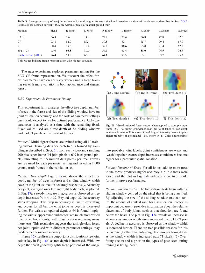
Figure 16 visualises the output joint distributions (see jointcolour key in Fig. 16a) as tree depth is increased. With lowdepth the forest generally splits large portions of the image

(a) (b) (c)

(d) (e) (f)

Fig. 16 Visualisation of forest output when applied to example inputframe (b). The output confidence map per joint label as tree depthincreases from 4 to 32 is shown in c–f. Higher intensity colour implieshigher probably of a joint label—key shown in (a) (Color figure online)

into probable joint labels. Joint confidences are weak and‘wash’ together. As tree depth increases, confidences becomehigher for a particular spatial location.

Results: Number of Trees For all joints, adding more treesto the forest produces higher accuracy. Up to 8 trees weretested and the plot in Fig. 17b indicates more trees couldfurther improve performance.

Results: Window Width The forest draws tests from within asliding window centred on the pixel that is being classified.By adjusting the size of the sliding window one can con-trol the amount of context used for classification. Context isimportant because it provides information about the relativeplacement of body joints, such as that shoulders are foundbelow the head. The plot in Fig. 17c reveals an increase inaccuracy as window width size is increased from 31 to 71 pix-els. A decline in accuracy is observed as the window widthis increased further. There are two possible reasons for thisbehaviour: (1) There are not enough test samples being drawnas the window width is increased past 71 pixels. (2) Over-fitting occurs and a prior on the types of pose seen duringtraining is being learnt.

123

Int J Comput Vis

Fig. 17 Accuracy of randomforest as a tree depth, b numberof trees in forest and c slidingwindow width are adjusted

4 32 64 128

40

60

80

100

Acc

urac

y (%

)(a) Tree depth

HeadWristsElbowsShouldersAverage

2 4 6 8

40

60

80

100

Acc

urac

y (%

)

(b) Number of trees

31 51 71 91 111

40

60

80

100

Acc

urac

y (%

)

(c) Window width (px)

2 4 6 8 10

40

60

80

100

Acc

urac

y (%

)

Number of training videos

Validation set

HeadWristsElbowsShouldersAverage

2 4 6 8 10 15

40

60

80

100

Number of training videos

Testing set

Fig. 18 Forest performance as amount of training data is increased.Results on validation set and testing set are shown

5.3.3 Experiment 3: Increasing Training Data

This experiment tests the intuition that more training datawill improve generalisation of the forest and hence increasethe accuracy of joint estimates.

Protocol Multiple forests are trained, each using a sampleof 2 videos from the set of 10 training videos. The SEG+CPframe representation and multi-signer forests are used. Forestparameters are optimised by maximising the average forestaccuracy when applied to the 1,000 ground truth frames inthe validation set. This process is repeated for a sample of4, 6, 8 and 10 training videos. The number of forests trainedfor each sample size is proportional to the total number ofpossible sample combinations (where the proportion con-stant is 1

21 ). E.g. for a sample size of 4 videos, we average

over⌈(

10C4)/21

⌉ = 10 videos. For a sample size of 2, 4,6, 8 and 10 videos, we averaged over 3, 10, 10, 3 and 1forest(s) respectively. Finally we also train a forest with 15videos using the testing and validation sets combined. Forthis forest, we are not able to tune parameters due to a lim-ited number of available videos. We therefore fix them atthe optimal parameters found when training with 10 videos.Seven hundred pixels per frame are sampled from 500 diverse

frames extracted from each of the sampled videos. All forestsare tested on 1,000 ground truth frames from videos in thetesting set.

Results Figure 18a shows the average accuracy achieved byforests on the validation set. For all joint types we observe ageneral increase in accuracy as more training data is added.The same trend is observed when applying these forests tounseen signers in the testing set as shown in Fig. 18b. Ofparticular interest is the drop in accuracy of the shoulderjoints when going from 8 to 10 videos. We believe this isdue to a particular video having noisy segmentations on thesigner’s left shoulder. It can also be noticed that elbows havehigher accuracy than wrists in the validation set, but viceversa on the testing set. This is due to more segmentationerrors at elbow locations in the testing videos.

5.3.4 Random Forest Versus State-of-the-Art

In this experiment the random forest is compared to Buehler etal.’s tracker and the deformable part based model by Yangand Ramanan (2011).

Protocol The forest is trained on the full 15 video trainingset. The optimal parameters from Sect. 5.3.2 are used, i.e. atree depth of 32, window size of 71 and 8 trees. The modelby Yang and Ramanan (2011) is trained for two differenttypes of video input: (1) The original RGB input, and (2) anRGB input with the background content removed by settingit to black. For both types of input the full 15 video datasetis used for training. From each video 100 diverse trainingframes were sampled, totaling 1,500 frames. Model parame-ters were set the same as those used for upper body poseestimation in Yang and Ramanan (2011). Negative trainingimages not containing people were taken from the INRIAdataset. Testing for all three upper body pose estimators isconducted on the full 5 video testing set.

Results Figure 19 shows accuracy as the allowed distancefrom ground truth is increased. The head accuracy and aver-

123

Int J Comput Vis

0 4 8 12 16 200

20

40

60

80

100

Acc

urac

y (%

)

Distance fromground truth (px)

Head

Buehler et al.Y&R input 1Y&R input 2Forest

0 4 8 12 16 200

20

40

60

80

100

Acc

urac

y (%

)Distance from

ground truth (px)

Wrists

0 4 8 12 16 200

20

40

60

80

100

Acc

urac

y (%

)

Distance fromground truth (px)

Elbows

0 4 8 12 16 200

20

40

60

80

100

Acc

urac

y (%

)

Distance fromground truth (px)

Shoulders

0 4 8 12 16 200

20

40

60

80

100

Acc

urac

y (%

)

Distance fromground truth (px)

Average

Fig. 19 Comparison of joint tracking accuracy of random forest trained on 15 videos against Buehler et al.’s tracker and Yang and Ramanan’spose estimation algorithm. Plots show accuracy per joint type (averaged over left and right body parts) as allowed distance from manual groundtruth is increased

Table 4 Average accuracy of per joint estimates on the full 5 video testing set. Estimates are deemed correct if they are within 5 pixels of manualground truth

Method Head R Wrist L Wrist R Elbow L Elbow R shldr L Shlder Average

Yang and Ramanan(2011) input 1

73.1 39.4 46.4 38.8 44.5 57.8 76.2 53.7

Yang and Ramanan(2011) input 2

59.3 28.3 39.6 15.2 19.1 46.4 18.7 32.4

Buehler et al. (2011) 97.0 53.9 70.6 41.6 60.2 73.8 75.1 67.5

Random forest 93.9 59.5 71.6 58.8 67.5 80.1 93.0 74.9

Bold values indicate method with highest accuracy

age accuracy over left and right joints are plotted. For alljoints but the head, the forest consistently performs betterthan Buehler et al.’s tracker. For the wrists and shoulders,erroneous joint predictions by the forest are further from theground truth than erroneous predictions from Buehler et al.’stracker once joint predictions are at least ≈ 10 pixels fromground truth. This fact means that it is likely to be easier fora pose evaluator to detect errors made by the forest. Inter-estingly, the model by Yang and Ramanan (2011) achievedbest performance when using the original RGB video input(input 1) over using a background removed version (input 2).We suggest that this is due to a poor representation of negativeimage patches in input 2 when using negative training imagesfrom the INRIA dataset. Overall, Yang and Ramanan’s modelis the least accurate over all joint types.

Table 4 shows per joint accuracy for Buehler et al.’s trackerand the forest using an allowed distance from ground truthof d = 5 pixels. The forest performs best with an averageaccuracy of 74.9 %. This suggests noisy data from Buehler etal.’s tracker is smoothed over by more consistent data at theleaf nodes of the trees. Results for the forest on an exam-ple 5 frames from the testing set is shown qualitatively inFig. 20.

5.4 Pose Evaluator

The pose evaluator is assessed here on the ability to label jointpredictions per frame as either success or fail. The quality of

joint predictions on success frames is also used as a measureof the evaluator’s performance.

Protocol The evaluator is trained on the validation set andtested on the test set shown in Fig. 11. For training, the jointtracking output from Buehler et al. (2011) is used to auto-matically label poses for a set of training frames as success orfail. For testing, the 1,000 frames with manual ground truth(described in Sect. 5.3.2) are used.

Results: Choice of Operating Point Figure 21a shows theROC curve of the evaluator when varying the operating point(effectively changing the threshold of the SVM classifier’sdecision function). This operating point determines the sen-sitivity at which the evaluator discards frames. The optimaloperating point occurs at a point on the curve which besttrades off false positives against true positives. This is a pointclosest to the top left hand corner of the plot. To gain furtherinsight into the effect of the operating point choice on jointestimates, we plot this value against joint prediction accuracyin Fig. 21b. This illustrates the correlation between the SVMscore and percentage of frames that the evaluator marks assuccesses (i.e. not failures). One can observe that when keep-ing the top 10 % frames, a 90 % average accuracy could beattained. More frames can be kept at the cost of loss in aver-age accuracy. The bump at 0.8 suggests that at a particularSVM score, the pose evaluator begins to remove some frameswhich may not contain a higher degree of error compared toframes removed with a higher SVM score threshold. How-

123

Int J Comput Vis

Fig. 20 Joint estimation results. Left shows colour model images, fromwhich we obtain probability densities of joint locations shown on topof the colour model edge image in centre. Different colours are usedper joint (higher intensity colour implies higher probability). Maximum

probability per joint is shown as grey crosses. Right shows a comparisonof estimated joints (filled in circles linked by a skeleton are) overlaid onfaded original frame, with ground truth joint locations (open circles)

123

Int J Comput Vis

0 0.2 0.4 0.6 0.8 10

0.1

0.2

0.3

0.4

0.5

0.6

0.7

0.8

0.9

1

false positive rate

true

pos

itive

rat

e (r

ecal

l)

ROC (AUC: 74.81%, EER: 31.06%)

ROCROC rand.

−1.6 −0.8 0 0.8 1.60

20

40

60

80

100

Acc

urac

y (%

)SVM score

HeadWristsElbowsShouldersAverage% of frames left

(b)(a)

Fig. 21 Pose evaluator classification performance. a ROC curve ofthe evaluator. b Change in accuracy as a function of the percentage offrames left after discarding frames that the evaluator detects as failures.For b the accuracy threshold is set as 5 pixels from manual ground truth

0 5 10 15 200

20

40

60

80

100

Acc

urac

y (%

)

Distance from ground truth (px)

Pre evaluator

HeadWristsElbowsShouldersAverage

0 5 10 15 200

20

40

60

80

100

Distance from ground truth (px)

Post evaluator

Fig. 22 Average accuracy of per-joint estimates without (left) and with(right) evaluator when the operating point of the pose evaluator is setto the optimum in Fig. 21a

ever, in general there is a positive correlation between theSVM score and pose estimation accuracy.

Results: Joint Localisation Figure 22 demonstrates theimprovement in joint localisation obtained by discardingframes that the evaluator classifies as failed. This yields an8.5 % increase in average accuracy (from 74.9 to 83.4 %) ata maximum distance of 5 pixels from ground truth, with 40.4% of the test frames remaining. One can observe a particu-larly significant improvement in wrist and elbow localisationaccuracy. This is due to a majority of hand mixup framesbeing correctly identified and filtered away. The improve-ments in other joints are due to the evaluator filtering awaymany frames where joints are assigned incorrectly due tosegmentation errors.

Results: Pose Visualisation A scatter plot of stickmen forthe forest joint predictions are plotted on all test frames inFig. 23a. Sticks are marked as orange if the elbow or wrist

(a) (b)

Fig. 23 a Shows scatter plots of stickmen for pose estimates fromforest on all training data. b Shows scatter plot of pose estimates fromforest on training data marked as containing good poses by the evaluator.Elbow and wrist joints greater than 5px from ground truth are indicatedby orange sticks (Color figure online)

joints are more than 5 pixels from ground truth. One observeserroneous joint predictions tend to exaggerate the length ofupper arms. Typically wrist joint errors occur when the wristsare further away from the torso centre. Figure 23b shows thesame plot as in Fig. 23a but only on testing frames markedas successful by the evaluator. Notice the evaluator has suc-cessfully removed errors on the elbows and wrists while stillretaining the majority of the correct poses.

5.5 Computation Time

The following computation times are on a 2.4 GHz Intel QuadCore I7 CPU with a 320 × 202 pixel image. The computa-tion time for one frame is 0.14 s for the co-segmentationalgorithm, 0.1 s for the random forest regressor and 0.1 s forthe evaluator, totalling 0.21 s (≈ 5fps). Face detection Zhuand Ramanan (2012) takes about 0.3 s/frame for a quad-core processor. The per-frame initialisation timings of theco-segmentation algorithm are 6 ms for finding the dynamicbackground layer and static background, 3 ms for obtaininga clean plate and 5 ms for finding the image sequence-wideforeground colour model, totalling 14 ms (approx. 24 minfor a 100 K frames). In comparison, Buehler et al.’s methodruns at 100 s per frame on a 1.83 GHz CPU, which is twoorders of magnitude slower. Each tree for our multi-signerRFs trained with 15 videos takes 20 h to train.

6 Conclusion

We have presented a fully automatic arm and hand tracker thatdetects joint positions over continuous sign language videosequences of more than an hour in length. Our frameworkattains superior performance to a state-of-the-art long termtracker Buehler et al. (2011), but does not require the man-ual annotation and, after automatic initialisation, performstracking in real-time on people that have not been seen dur-ing training. Moreover, our framework augments the jointestimates with a failure prediction score, enabling incorrect

123

Int J Comput Vis

poses to be filtered away. Future work includes improvingthe evaluator by adding new features, and using its outputnot only as an indication of failure but also as an evaluationmeasure to help correct failed poses.

Acknowledgments We are grateful to Lubor Ladicky for discussions,and to Patrick Buehler for his very generous help. Funding is providedby the Engineering and Physical Sciences Research Council (EPSRC)grant Learning to Recognise Dynamic Visual Content from BroadcastFootage.

References

Amit, Y., & Geman, D. (1997). Shape quantization and recognition withrandomized trees. Neural Computation, 9(7), 1545–1588.

Andriluka, M., Roth, S., & Schiele, B. (2012). Discriminative appear-ance models for pictorial structures. International Journal of Com-puter Vision, 99(3), 259–280.

Apostoloff, N. E., & Zisserman, A. (2007). Who are you?—real-timeperson identification. In Proceedings of the British machine visionconference.

Benfold, B., & Reid, I. (2008). Colour invariant head pose classificationin low resolution video. In Proceedings of the British machine visionconference.

Bosch, A., Zisserman, A., & Munoz, X. (2007). Image classificationusing random forests and ferns. In Proceedings of the internationalconference on computer vision.

Bowden, R., Windridge, D., Kadir, T., Zisserman, A., & Brady, J. M.(2004). A linguistic feature vector for the visual interpretation of signlanguage. In Proceedings of the European conference on computervision. Berlin: Springer.

Breiman, L. (2001). Random forests. Machine Learning, 45(1), 5–32.Buehler, P., Everingham, M., Huttenlocher, D. P., & Zisserman, A.

(2011). Upper body detection and tracking in extended signingsequences. International Journal of Computer Vision, 95(2), 180–197.

Buehler, P., Everingham, M., & Zisserman, A. (2009). Learning signlanguage by watching TV (using weakly aligned subtitles). In Pro-ceedings of the IEEE conference on computer vision and patternrecognition.

Buehler, P., Everingham, M., & Zisserman, A. (2010). Employingsigned TV broadcasts for automated learning of British sign lan-guage. In Workshop on representation and processing of sign lan-guages.

Chai, Y., Lempitsky, V., & Zisserman, A. (2011). BiCoS: A bi-levelco-segmentation method for image classification. In Proceedings ofthe international conference on computer vision.

Chai, Y., Rahtu, E., Lempitsky, V., Van Gool, L., & Zisserman,A. (2012). Tricos: A tri-level class-discriminative co-segmentationmethod for image classification. In European conference on com-puter vision.

Charles, J., Pfister, T., Magee, D., Hogg, D., & Zisserman, A. (2013).Domain adaptation for upper body pose tracking in signed TV broad-casts. In Proceedings of the British machine vision conference.

Chunli, W., Wen, G., & Jiyong, M. (2002). A real-time large vocabularyrecognition system for Chinese Sign Language. Gesture and signlanguage in HCI.

Cooper, H., & Bowden, R. (2007). Large lexicon detection of sign lan-guage. Workshop on human computer interaction.

Cooper, H., & Bowden, R. (2009). Learning signs from subtitles: Aweakly supervised approach to sign language recognition. In Pro-ceedings of the IEEE conference on computer vision and patternrecognition.

Cootes, T., Ionita, M., Lindner, C., & Sauer, P. (2012). Robust andaccurate shape model fitting using random forest regression voting.In Proceedings of the European conference on computer vision.

Criminisi, A., Shotton, J., & Konukoglu, E. (2012). Decision forests: Aunified framework for classification, regression, density estimation,manifold learning and semi-supervised learning. Foundations andTrends in Computer Graphics and Vision, 7(2), 81–227.

Criminisi, A., Shotton, J., & Robertson, & D., Konukoglu, E., (2011).Regression forests for efficient anatomy detection and localization inCT studies. In International conference on medical image comput-ing and computer assisted intervention workshop on probabilisticmodels for medical image analysis.

Dalal, N., & Triggs, B. (2005). Histogram of Oriented Gradients forHuman Detection. In Proceedings of the IEEE conference on com-puter vision and pattern recognition.

Dantone, M., Gall, J., Fanelli, G., & Van Gool, L. (2012). Real-timefacial feature detection using conditional regression forests. In Pro-ceedings of the IEEE conference on computer vision and patternrecognition.

Dreuw, P., Deselaers, T., Rybach, D., Keysers, D., & Ney, H. (2006).Tracking using dynamic programming for appearance-based signlanguage recognition. In Proceedings of the IEEE conference onautomatic face and gesture recognition.

Dreuw, P., Forster, J., & Ney, H. (2012). Tracking benchmark databasesfor video-based sign language recognition. In Trends and topics incomputer vision (pp. 286–297). Berlin: Springer.

Eichner, M., & Ferrari, V. (2009). Better appearance models forpictorial structures. In Proceedings of the British machine visionconference.

Eichner, M., Marin-Jimenez, M., Zisserman, A., & Ferrari, V. (2012).2D articulated human pose estimation and retrieval in (almost)unconstrained still images. International Journal of ComputerVision, 1–25.

Fanelli, G., Dantone, M., Gall, J., Fossati, A., & Van Gool, L. (2012).Random forests for real time 3D face analysis. International Journalof Computer Vision, 101(3), 1–22.

Fanelli, G., Gall, J., & Van Gool, L. (2011). Real time head pose esti-mation with random regression forests. In Proceedings of the IEEEconference on computer vision and pattern recognition.

Farhadi, A., & Forsyth, D. (2006). Aligning asl for statistical transla-tion using a discriminative word model. In Proceedings of the IEEEconference on computer vision and pattern recognition.

Farhadi, A., Forsyth, D., & White, R. (2007). Transfer learning in signlanguage. In Proceedings of the IEEE conference on computer visionand pattern recognition.

Felzenszwalb, P., Girshick, R., & McAllester, D. (2010). Cascade objectdetection with deformable part models. In Proceedings of the IEEEconference on computer vision and pattern recognition.

Felzenszwalb, P., & Huttenlocher, D. (2005). Pictorial structures forobject recognition. International Journal of Computer Vision, 61(1),55–79.

Felzenszwalb, P., McAllester, D., & Ramanan, D. (2008). A discrimi-natively trained, multiscale, deformable part model. In Proceedingsof the IEEE conference on computer vision and pattern recognition.

Ferrari, V., Marin-Jimenez, M., & Zisserman, A. (2008). Progressivesearch space reduction for human pose estimation. In Proceedingsof the IEEE conference on computer vision and pattern recognition.

Gall, J., & Lempitsky, V. (2009). Class-specific hough forests for objectdetection. In Proceedings of the IEEE conference on computer visionand pattern recognition.

Geremia, E., Clatz, O., Menze, B., Konukoglu, E., Criminisi, A., &Ayache, N. (2011). Spatial decision forests for MS lesion segmen-tation in multi-channel magnetic resonance images. NeuroImage,57(2), 378–390.

Girshick, R., Shotton, J., Kohli, P., Criminisi, A., & Fitzgibbon, A.(2011). Efficient regression of general-activity human poses from

123

Int J Comput Vis

depth images. In Proceedings of the international conference oncomputer vision.

Hochbaum, D., & Singh, V. (2009). An efficient algorithm for co-segmentation. In Proceedings of the international conference oncomputer vision.

Jammalamadaka, N., Zisserman, A., Eichner, M., Ferrari, V., & Jawa-har, C. V. (2012). Has my algorithm succeeded? An evaluator forhuman pose estimators. In Proceedings of the European conferenceon computer vision.

Johnson, S., & Everingham, M. (2009). Combining discriminativeappearance and segmentation cues for articulated human pose esti-mation. In IEEE international workshop on machine learning forvision-based motion analysis.

Jojic, N., & Frey, B. (2001). Learning flexible sprites in video layers. InProceedings of the IEEE conference on computer vision and patternrecognition.

Joulin, A., Bach, F., & Ponce, J. (2010). Discriminative clustering forimage co-segmentation. In Proceedings of the IEEE conference oncomputer vision and pattern recognition.

Kadir, T., Bowden, R., Ong, E., & Zisserman, A. (2004). Minimal train-ing, large lexicon, unconstrained sign language recognition. In Pro-ceedings of the British machine vision conference.

Kadir, T., Zisserman, A., & Brady, J. M. (2004). An affine invariantsalient region detector. In Proceedings of the European conferenceon computer vision.

Kontschieder, P., Bulò, S., Criminisi, A., Kohli, P., Pelillo, M., &Bischof, H. (2012). Context-sensitive decision forests for objectdetection. In Advances in neural information processing systems.

Kumar, M. P., Torr, P. H. S., & Zisserman, A. (2008). Learning layeredmotion segmentations of video. International Journal of ComputerVision, 76, 301–319.

Lepetit, V., & Fua, P. (2006). Keypoint recognition using randomizedtrees. IEEE Transactions on Pattern Analysis and Machine Intelli-gence, 28(9), 1465–1479.

Liu, C., Gong, S., Loy, C., & Lin, X. (2012). Person re-identification:What features are important?. In Proceedings of the European con-ference on computer vision.

Marée, R., Geurts, P., Piater, J., & Wehenkel, L. (2005). Random sub-windows for robust image classification. In Proceedings of the IEEEconference on computer vision and pattern recognition.

Moeslund, T. (2011). Visual analysis of humans: Looking at people.Berlin: Springer.

Nowozin, S., Rother, C., Bagon, S., Sharp, T., Yao, B., & Kohli, P.(2011). Decision tree fields. In Proceedings of the international con-ference on computer vision.

Ong, E., & Bowden, R. (2004). A boosted classifier tree for hand shapedetection. In Proceedings of the international conference on auto-matic face and gesture recognition.

Ozuysal, M., Calonder, M., Lepetit, V., & Fua, P. (2010). Fast key-point recognition using random ferns. IEEE Transactions on PatternAnalysis and Machine Intelligence, 32(3), 448–461.

Pfister, T., Charles, J., Everingham, M., & Zisserman, A. (2012). Auto-matic and efficient long term arm and hand tracking for continuoussign language TV broadcasts. In Proceedings of the British machinevision conference.

Pfister, T., Charles, J., & Zisserman, A. (2013). Large-scale learning ofsign language by watching TV (using co-occurrences). In Proceed-ings of the British machine vision conference.

Ramanan, D. (2006). Learning to parse images of articulated bodies. InAdvances in neural information processing systems.

Ramanan, D., Forsyth, D. A., & Zisserman, A. (2007). Tracking peopleby learning their appearance. IEEE Transactions on Pattern Analysisand Machine Intelligence, 29(1), 65–81.

Rother, C., Kolmogorov, V., & Blake, A. (2004). Grabcut: interactiveforeground extraction using iterated graph cuts. In Proceedings ofthe ACM SIGGRAPH conference on computer graphics.

Rother, C., Minka, T., Blake, A., & Kolmogorov, V. (2006). Cosegmen-tation of image pairs by histogram matching-incorporating a globalconstraint into MRFs. In Proceedings of the IEEE conference oncomputer vision and pattern recognition.

Santner, J., Leistner, C., Saffari, A., Pock, T., & Bischof, H. (2010).Prost: Parallel robust online simple tracking. In Proceedings of theIEEE conference on computer vision and pattern recognition.

Sapp, B., Jordan, C., & Taskar, B. (2010). Adaptive pose priors for pic-torial structures. In Proceedings of the IEEE conference on computervision and pattern recognition.

Sapp, B., Weiss, D., & Taskar, B. (2011). Parsing human motion withstretchable models. In Proceedings of the IEEE conference on com-puter vision and pattern recognition.

Sharp, T. (2008). Implementing decision trees and forests on a GPU. InProceedings of the European conference on computer vision.

Shotton, J., Fitzgibbon, A., Cook, M., Sharp, T., Finocchio, M., Moore,R., et al. (2011). Real-time human pose recognition in parts fromsingle depth images. In Proceedings of the IEEE conference on com-puter vision and pattern recognition.

Shotton, J., Johnson, M., & Cipolla, R. (2008). Semantic texton forestsfor image categorization and segmentation. In Proceedings of theIEEE conference on computer vision and pattern recognition.

Sivic, J., Zitnick, C. L., & Szeliski, R. (2006). Finding people in repeatedshots of the same scene. In Proceedings of the British machine visionconference, Edinburgh.

Starner, T., Weaver, J., & Pentland, A. (1998a). Real-time americansign language recognition using desk- and wearable computer-basedvideo. IEEE Transactions on Pattern Analysis and Machine Intelli-gence, 20(12), 1371–1375.

Starner, T., Weaver, J., & Pentland, A. (1998b). Real-time AmericanSign Language recognition using desk and wearable computer basedvideo. IEEE Transactions on Pattern Analysis and Machine Intelli-gence, 20(12), 1371–1375.

Sun, M., Kohli, P., & Shotton, J. (2012). Conditional regression forestsfor human pose estimation. In Proceedings of the IEEE conferenceon computer vision and pattern recognition.

Szeliski, R., Avidan, S., & Anandan, P. (2000). Layer extraction frommultiple images containing reflections and transparency. In Proceed-ings of the IEEE conference on computer vision and pattern recog-nition.

Taylor, J., Shotton, J., Sharp, T., & Fitzgibbon, A. (2012). The vitru-vian manifold: Inferring dense correspondences for one-shot humanpose estimation. In Proceedings of the IEEE conference on computervision and pattern recognition.

Tran, D., & Forsyth, D. (2010). Improved human parsing with a fullrelational model. In Proceedings of the European conference on com-puter vision.

Vogler, C., & Metaxas, D. (1998). ASL recognition based on a cou-pling between HMMs and 3D motion analysis. In Proceedings ofthe international conference on computer vision.

Yang, Y., & Ramanan, D. (2011). Articulated pose estimation with flex-ible mixtures-of-parts. In Proceedings of the IEEE conference oncomputer vision and pattern recognition.

Yin, P., Criminisi, A., Winn, J., & Essa, I. (2007). Tree-based classi-fiers for bilayer video Segmentation. In Proceedings of the IEEEconference on computer vision and pattern recognition.

Zhu, X., & Ramanan, D. (2012). Face detection, pose estimation, andlandmark localization in the wild. In Proceedings of the IEEE con-ference on computer vision and pattern recognition.

Zisserman, A., Winn, J., Fitzgibbon, A., van Gool, L., Sivic, J.,Williams, C., & Hogg, D. (2012). In memoriam: Mark Everingham.IEEE Transactions on Pattern Analysis and Machine Intelligence,34(11), 2081–2082.

123