Automated Test Case Generation to Validate Non-functional Software Requirements

University of Nebraska - LincolnDigitalCommons@University of Nebraska - LincolnComputer Science and Engineering: Theses,Dissertations, and Student Research Computer Science and Engineering, Department of

Summer 8-16-2013

Automated Test Case Generation to Validate Non-functional Software RequirementsPingyu ZhangUniversity of Nebraska - Lincoln, [email protected]

Follow this and additional works at: http://digitalcommons.unl.edu/computerscidiss

Part of the Software Engineering Commons

This Article is brought to you for free and open access by the Computer Science and Engineering, Department of at DigitalCommons@University ofNebraska - Lincoln. It has been accepted for inclusion in Computer Science and Engineering: Theses, Dissertations, and Student Research by anauthorized administrator of DigitalCommons@University of Nebraska - Lincoln.

Zhang, Pingyu, "Automated Test Case Generation to Validate Non-functional Software Requirements" (2013). Computer Science andEngineering: Theses, Dissertations, and Student Research. 62.http://digitalcommons.unl.edu/computerscidiss/62

http://digitalcommons.unl.edu?utm_source=digitalcommons.unl.edu%2Fcomputerscidiss%2F62&utm_medium=PDF&utm_campaign=PDFCoverPages

http://digitalcommons.unl.edu/computerscidiss?utm_source=digitalcommons.unl.edu%2Fcomputerscidiss%2F62&utm_medium=PDF&utm_campaign=PDFCoverPages


http://digitalcommons.unl.edu/computerscienceandengineering?utm_source=digitalcommons.unl.edu%2Fcomputerscidiss%2F62&utm_medium=PDF&utm_campaign=PDFCoverPages


http://network.bepress.com/hgg/discipline/150?utm_source=digitalcommons.unl.edu%2Fcomputerscidiss%2F62&utm_medium=PDF&utm_campaign=PDFCoverPages

http://digitalcommons.unl.edu/computerscidiss/62?utm_source=digitalcommons.unl.edu%2Fcomputerscidiss%2F62&utm_medium=PDF&utm_campaign=PDFCoverPages

AUTOMATED TEST CASE GENERATION TO VALIDATE

NON-FUNCTIONAL SOFTWARE REQUIREMENTS

by

Pingyu Zhang

A DISSERTATION

Presented to the Faculty of

The Graduate College at the University of Nebraska

In Partial Fulfillment of Requirements

For the Degree of Doctor of Philosophy

Major: Computer Science

Under the Supervision of Professor Sebastian Elbaum

Lincoln, Nebraska

August, 2013

AUTOMATED TEST CASE GENERATION TO VALIDATE

NON-FUNCTIONAL SOFTWARE REQUIREMENTS

Pingyu Zhang, Ph.D.

University of Nebraska, 2013

Advisor: Sebastian Elbaum

A software system is bounded by a set of requirements. Functional requirements

describe what the system must do, in terms of inputs, behavior, and outputs. We

define non-functional requirements to be how well these functional requirements are

satisfied, in terms of qualities or constraints on the design or on the implementation of

a system. In practice, the validation of these kinds of requirements, does not receive

equal emphasis. Techniques for validating functional requirements target all levels

of software testing phases, and explore both black-box and white-box approaches.

Techniques for validating non-functional requirements, on the other hand, largely

operate in a black-box manner, and focus mostly on system testing level. As a result,

in practice more efforts are focused on validating functional requirements, and only

assess non-functional requirements after functional validation is complete.

In this dissertation, we propose a set of automated bounded exhaustive white-box

testing techniques that enable cost-effective validation of non-functional requirements

from two perspectives. For non-functional requirements defined as qualities of a sys-

tem, we target load testing for the purpose of performance validation. We present

Symbolic Load Generation (SLG), a load test suite generation approach that uses

symbolic execution to exhaustively traverse program execution paths, and produce

test cases for the ones that may expose worst-case or near worst-case resource con-

sumption scenarios. An assessment of SLG on a set of Java applications shows that it

generates test suites that induce program response times and memory consumption

several times worse than the compared alternatives, it scales to large and complex

inputs, and it exposes a diversity of resource consuming program behavior. We subse-

quently present CompSLG, a compositional load test generation technique that aims

to achieve better scalability than SLG. CompSLG is fully automated to handle soft-

ware that follows the pipeline architecture, and is evaluated on a group of Unix and

XML pipelines. The results show that it generates load tests in situations where SLG

fails to scale, and achieves comparable load with a fraction of the cost. We also ex-

tend CompSLG to enable the handling of more complex software structures in terms

of Java programs, and show the viability of the extended technique through a series

of examples.

For non-functional requirements defined as constraints on a system, we target val-

idation of contextual constraints that are imposed by external resources with which

the software interacts. We first assessed the magnitude of the problem by conducting

a study on fault repositories of several popular Android applications. We then present

an approach that amplifies existing tests in an exhaustive manner to validate excep-

tion handling constructs that are used to handle such constraints. Our assessment of

the approach on a set of Android mobile applications indicates that it can be fully

automated, is powerful enough to detect 67% of the faults reported in the bug reports

of this kind, and is precise enough that 78% of the detected anomalies correspond to

faults fixed by the developers.

Combined, the two proposed techniques advance the field of automated software

testing by providing white-box support for non-functional validation.

ACKNOWLEDGEMENTS

First and foremost I would like to express my sincere gratitude and appreciation to my

advisor, Dr. Sebastian Elbaum, for the guidance, inspiration, suggestions, criticism,

and financial support that he has provided throughout the course of my research

and studies. He not only shaped my problem solving capabilities in academics, but

also carried me through difficult times during this six-year journey. This dissertation

would not be a reality without the countless support from him.

Special thanks are also extended to Dr. Berthe Choueiry, Dr. Michael Dodd,

and Dr. Matthew Dwyer, for taking the time to review this dissertation and serving

on my doctoral advisory committee. In particular, I would like to acknowledge and

thank Matthew Dwyer, with whom I had the honor to co-author several papers that

eventually made their way to this dissertation. Working with him is an enjoyable

experience, and I benefited a lot from his impressive depth and breadth of knowledge.

I am also grateful to the research institutes, for which I had the honor to work

through several internships during the course of my studies. Among those are NASA

Ames Research Center in California, and ABB Corporate Research in Raleigh, North

Carolina.

To the people in the ESQuaRed Laboratory at the University of Nebraska-Lincoln,

you have provided a superb working atmosphere. Special thanks to my officemates

Wayne Motycka and Zhihong Xu, for making this six-year journey a little bit more

enjoyable.

My parents have been a continuous source of support for me through out the

years. To each of them, I am deeply grateful.

And finally, I would like to thank my wife, Wei Liu. Her love, support and

encouragement have made it possible for me to achieve this dream. Thank you for

believing in me.

This material is based in part upon work supported by NSF Award CCF-0915526,

and by AFOSR Award #FA9550-10-1-0406. Any opinions, findings, and conclusions

or recommendations expressed in this material are those of the author(s) and do not

necessarily reflect the views of AFOSR or NSF.

vi

Contents

1 Introduction 11.1 Motivation . . . . . . . . . . . . . . . . . . . . . . . . . . . . . . . . . 11.2 Non-functional Requirement Validation: Load Testing . . . . . . . . . 51.3 Non-functional Requirement Validation: Exception Handling . . . . . 81.4 Dissertation Statement . . . . . . . . . . . . . . . . . . . . . . . . . . 101.5 Contributions of this Research . . . . . . . . . . . . . . . . . . . . . . 111.6 Outline of Dissertation . . . . . . . . . . . . . . . . . . . . . . . . . . 13

2 Background & Related Work 142.1 Symbolic Execution . . . . . . . . . . . . . . . . . . . . . . . . . . . . 14

2.1.1 Generalized Symbolic Execution . . . . . . . . . . . . . . . . . 172.1.2 Dynamic Symbolic Execution . . . . . . . . . . . . . . . . . . 192.1.3 Using Symbolic Execution for Automatic Test Generation . . 202.1.4 Search Heuristics in Symbolic Execution . . . . . . . . . . . . 242.1.5 Memoization in Symbolic Execution . . . . . . . . . . . . . . . 25

2.2 Automated Techniques for Load Testing . . . . . . . . . . . . . . . . 272.2.1 Generating Load Tests . . . . . . . . . . . . . . . . . . . . . . 282.2.2 Identifying Performance Problems . . . . . . . . . . . . . . . . 30

2.3 Techniques for Detecting Faults in Exception Handling Code . . . . . 342.3.1 Mining Specifications of Exceptional Behavior . . . . . . . . . 342.3.2 Exceptional Control Flow Representation . . . . . . . . . . . . 352.3.3 Fault Injection . . . . . . . . . . . . . . . . . . . . . . . . . . 362.3.4 Mocking . . . . . . . . . . . . . . . . . . . . . . . . . . . . . . 37

3 Automatic Generation of Load Tests 393.1 Challenges . . . . . . . . . . . . . . . . . . . . . . . . . . . . . . . . . 393.2 Approach Overview . . . . . . . . . . . . . . . . . . . . . . . . . . . . 413.3 The SLG Algorithm . . . . . . . . . . . . . . . . . . . . . . . . . . . 44

3.3.1 Parameterizing SLG . . . . . . . . . . . . . . . . . . . . . . . 473.3.2 Clustering the Frontier and Diversity Checks . . . . . . . . . . 513.3.3 Dealing with Solver Limitations . . . . . . . . . . . . . . . . . 52

3.4 Implementation . . . . . . . . . . . . . . . . . . . . . . . . . . . . . . 543.5 Evaluation . . . . . . . . . . . . . . . . . . . . . . . . . . . . . . . . . 56

3.5.1 Revealing Response Time Issues . . . . . . . . . . . . . . . . . 573.5.2 Revealing Memory Consumption Issues . . . . . . . . . . . . . 613.5.3 Load inducing tests across resources and test diversity . . . . 62

3.6 Summary . . . . . . . . . . . . . . . . . . . . . . . . . . . . . . . . . 64

4 Compositional Load Test Generation 654.1 Motivation . . . . . . . . . . . . . . . . . . . . . . . . . . . . . . . . . 66

4.1.1 Software Pipelines . . . . . . . . . . . . . . . . . . . . . . . . 664.1.2 Challenges in Load Testing Pipelines . . . . . . . . . . . . . . 68

4.2 Overview of a Compositional Approach . . . . . . . . . . . . . . . . . 704.3 The CompSLG Algorithm . . . . . . . . . . . . . . . . . . . . . . . . 73

4.3.1 Selecting Compatible Path Conditions . . . . . . . . . . . . . 764.3.2 Generating Channeling Constraints . . . . . . . . . . . . . . . 784.3.3 Weighing and Relaxing Constraints . . . . . . . . . . . . . . . 794.3.4 Handling Split Pipelines . . . . . . . . . . . . . . . . . . . . . 82

4.4 Implementation . . . . . . . . . . . . . . . . . . . . . . . . . . . . . . 824.5 Evaluation . . . . . . . . . . . . . . . . . . . . . . . . . . . . . . . . . 83

4.5.1 Artifacts . . . . . . . . . . . . . . . . . . . . . . . . . . . . . . 844.5.2 Metrics and Treatments . . . . . . . . . . . . . . . . . . . . . 864.5.3 Experiment Setup . . . . . . . . . . . . . . . . . . . . . . . . . 874.5.4 Results and Analysis . . . . . . . . . . . . . . . . . . . . . . . 88

4.6 Exploring CompSLG Extensions to Richer Structures . . . . . . . . . 914.6.1 Richer Channeling Constraints . . . . . . . . . . . . . . . . . . 94

4.6.1.1 Approach to Capture CCr and CCw . . . . . . . . . 944.6.1.2 Putting It All Together . . . . . . . . . . . . . . . . 994.6.1.3 Proof-of-Concept Examples . . . . . . . . . . . . . . 101

4.6.2 Richer Performance Summaries . . . . . . . . . . . . . . . . . 1144.6.2.1 Revisiting the Approach to Generating Performance

Summaries . . . . . . . . . . . . . . . . . . . . . . . 1174.6.3 A New Strategy for Summary Composition . . . . . . . . . . . 121

4.6.3.1 Revisiting the Approach to Composition . . . . . . . 1214.7 Summary . . . . . . . . . . . . . . . . . . . . . . . . . . . . . . . . . 124

5 Amplifying Tests to Validate Exception Handling Code 1265.1 Magnitude of the Problem . . . . . . . . . . . . . . . . . . . . . . . . 1275.2 Difficulties in Exposing Faulty Exceptional Behavior . . . . . . . . . . 1315.3 Test Amplification . . . . . . . . . . . . . . . . . . . . . . . . . . . . 135

5.3.1 Overview with Example . . . . . . . . . . . . . . . . . . . . . 1355.3.2 Problem Definition . . . . . . . . . . . . . . . . . . . . . . . . 1385.3.3 Approach Architecture . . . . . . . . . . . . . . . . . . . . . . 1405.3.4 Implementation . . . . . . . . . . . . . . . . . . . . . . . . . . 143

5.4 Evaluation . . . . . . . . . . . . . . . . . . . . . . . . . . . . . . . . . 1455.4.1 Study Design and Implementation . . . . . . . . . . . . . . . . 146

vii

viii

5.4.2 RQ1: Cost Effectiveness in Detecting Anomalies . . . . . . . . 1485.4.2.1 Results with Mocking Length=10 . . . . . . . . . . . 1485.4.2.2 Controlling the Mocking Length Parameter for Cost

Effectiveness . . . . . . . . . . . . . . . . . . . . . . 1505.4.2.3 A Closer Look at the Mocking Patterns . . . . . . . 153

5.4.3 RQ2: Anomalies & Failures . . . . . . . . . . . . . . . . . . . 1555.4.3.1 Precision and Recall . . . . . . . . . . . . . . . . . . 1555.4.3.2 Feedback From Application Developers . . . . . . . . 159

5.4.4 Threats to Validity . . . . . . . . . . . . . . . . . . . . . . . . 1615.4.5 Extended Domain and Alternative Approach . . . . . . . . . . 1615.4.6 Preliminary Case Study . . . . . . . . . . . . . . . . . . . . . 163

5.5 Summary . . . . . . . . . . . . . . . . . . . . . . . . . . . . . . . . . 164

6 Conclusions and Future Work 1666.1 Summary and Impact . . . . . . . . . . . . . . . . . . . . . . . . . . . 1666.2 Limitations . . . . . . . . . . . . . . . . . . . . . . . . . . . . . . . . 1706.3 Future Work . . . . . . . . . . . . . . . . . . . . . . . . . . . . . . . . 174

Bibliography 177

ix

List of Figures

2.1 Code fragment for foo() and its corresponding symbolic execution tree. . . 15

3.1 SQL query template. . . . . . . . . . . . . . . . . . . . . . . . . . . . . 403.2 Histogram of response time for TinySQL. . . . . . . . . . . . . . . . . . 413.3 Iterative-deepening beam symbolic execution. . . . . . . . . . . . . . . . 433.4 Quality of load tests as a function of lookAhead. . . . . . . . . . . . . . 493.5 Illustration of the SLG implementation. . . . . . . . . . . . . . . . . . . 543.6 Revealing performance issues: response time differences of JZlib vs Zlib

when using testing suites generated by CLLG vs Random. . . . . . . . . 583.7 Scaling: response times of JZlib with test suites generated by CLLG and

Random. . . . . . . . . . . . . . . . . . . . . . . . . . . . . . . . . . . 60

4.1 Pipeline structures. . . . . . . . . . . . . . . . . . . . . . . . . . . . . . 664.2 Illustration of a compositional approach. . . . . . . . . . . . . . . . . . . 704.3 Path constraints computed for grep [pattern] file | sort, with the

pattern being a 10-digit phone number. Three sets of constraints are shown,

one for grep, one for sort, one for the channeling constraints connecting

them. Crossed out constraints have been removed in order to find a solution. 724.4 Symbolic file modeling. . . . . . . . . . . . . . . . . . . . . . . . . . . . 754.5 Cost-effectiveness of treatments applied to Unix pipelines. Triangles repre-

sent CompSLG (blank for No-reuse, shaded for Incremental-reuse, solid for

Full-reuse), diamonds represent SLG, and the circles represent Random. . 894.6 Cost-effectiveness of treatments applied to XML pipeline. Triangles repre-

sent CompSLG (blank for No-reuse, solid for Full-reuse), diamonds represent

SLG, and the circles represent Random. . . . . . . . . . . . . . . . . . . 904.7 Custom-SE Applied to Example Code. . . . . . . . . . . . . . . . . . . 984.8 Illustration of a compositional approach for Java programs. . . . . . . . . 994.9 Code example 1: single function call, no side effects. . . . . . . . . . . . 1034.10 Code example 2: single function call, with side effects. . . . . . . . . . . 1054.11 Code example 3: multiple function calls, with side effects. . . . . . . . . 1064.12 Code example 4: multiple function calls, with side effects and a predicate. 1084.13 Code example 5: multiple nested function calls, with side effects. . . . . . 1114.14 Code snippet for the AVL tree: five inserts. . . . . . . . . . . . . . . . . 1154.15 Code snippet for the AVL tree: eight calls. . . . . . . . . . . . . . . . . . 119

x

5.1 Code excerpt (with comments added for readability) from XBMC Remote

Revision 220 with a faulty exception handling mechanism. . . . . . . . . 1325.2 Submitted fix to the previous code in Revision 317. . . . . . . . . . . . . 1345.3 Illustration of test amplification up to length 5. Each path from the root

to a leaf corresponds to a mocking pattern. 32 patterns are explored and 4

failing patterns (marked as FP1-FP4) are found. . . . . . . . . . . . . . 1365.4 Failure report corresponding to FP1. . . . . . . . . . . . . . . . . . . . . 1375.5 Amplification architecture. . . . . . . . . . . . . . . . . . . . . . . . . . 1415.6 Excerpts of aspect for online mocking and error injection. . . . . . . . . . 1445.7 Anomalies detected by Tamp under various mocking lengths for application-

resource combinations. Each observation corresponds to a mocking length

(from left to right: 1, 3, 5, 7, and 10). X-axis represents cost in terms

of execution time in hours, and Y-axis represents the number of anomalies

detected. . . . . . . . . . . . . . . . . . . . . . . . . . . . . . . . . . 1525.8 Categorization of mocking patterns. . . . . . . . . . . . . . . . . . . . . 1545.9 Mapping detected anomalies to bug reports. . . . . . . . . . . . . . . . 1575.10 Mapping bug reports to anomalies. . . . . . . . . . . . . . . . . . . . . 158

xi

List of Tables

3.1 Load test generation for memory consumption. . . . . . . . . . . . . . . 623.2 Response time and memory consumption for test suites designed to increase

those performance measures in isolation (TS-RT and TS-MEM) and jointly

(TS-RT-MEM). . . . . . . . . . . . . . . . . . . . . . . . . . . . . . . . 623.3 Queries illustrating test suite diversity. . . . . . . . . . . . . . . . . . . . 64

4.1 SLG on the pipeline grep [pattern] file | sort with increasing input

sizes. . . . . . . . . . . . . . . . . . . . . . . . . . . . . . . . . . . . . 694.2 SLG on pipelines of increasing complexity. . . . . . . . . . . . . . . . . . 694.3 Compositional approach on the pipeline grep [pattern] file | sort with

increasing input size. % in Gen. and Load shows comparison to Table 4.1. 734.4 Compositional approach on pipelines with increasing complexity Previously

computed summaries are reused. % in Gen. and Load shows comparison to

Table 4.2. . . . . . . . . . . . . . . . . . . . . . . . . . . . . . . . . . . 734.5 Illustration of weighing and relaxing constraints. White areas correspond

to the original weight, shaded areas correspond to the adjusted weights. . 814.6 Unix and XML programs. . . . . . . . . . . . . . . . . . . . . . . . . . 844.7 Summary of pipeline artifacts. . . . . . . . . . . . . . . . . . . . . . . . 854.8 Handling pipelines vs. Java programs. . . . . . . . . . . . . . . . . . . . 924.9 Summary of the proof–of-concept examples. . . . . . . . . . . . . . . . . 1024.10 Constraint composition for code example 1. . . . . . . . . . . . . . . . . 1044.11 Constraint composition for code example 2. . . . . . . . . . . . . . . . . 1064.12 Constraint composition for code example 3. . . . . . . . . . . . . . . . . 1074.13 Constraint composition for code example 4 (Path 1). . . . . . . . . . . . 1094.14 Constraint composition for code example 4 (Path 2). . . . . . . . . . . . 1104.15 Constraint composition for code example 5 (Path 1). . . . . . . . . . . . 1124.16 Constraint composition for code example 5 (Path 2). . . . . . . . . . . . 1134.17 Handling AVL tree with five inserts (size match). . . . . . . . . . . . . . 1164.18 Handling AVL tree with five inserts (shape match). . . . . . . . . . . . . 1174.19 Evaluation: AVL tree with five inserts. . . . . . . . . . . . . . . . . . . . 1174.20 Handling AVL tree with eight calls. . . . . . . . . . . . . . . . . . . . . 1204.21 Evaluation of the AVL tree example continued. . . . . . . . . . . . . . . 120

5.1 Summary of artifacts. . . . . . . . . . . . . . . . . . . . . . . . . . . . 128

xii

5.2 Classification of confirmed and fixed bug reports. . . . . . . . . . . . . . 1295.3 Characterization of the original test suites. . . . . . . . . . . . . . . . . 1495.4 Characterization of the amplified test suites. . . . . . . . . . . . . . . . 1505.5 Anomalies detected. . . . . . . . . . . . . . . . . . . . . . . . . . . . . 1515.6 Summary of feedbacks from developers. . . . . . . . . . . . . . . . . . . 160

6.1 Summary of limitations. . . . . . . . . . . . . . . . . . . . . . . . . . . 171

1

Chapter 1

Introduction

In this chapter, we first present the motivation for the research efforts that lead to

this dissertation, then summaries the contributions of this research.

1.1 Motivation

A software system, from its inception, is bounded by a set of requirements. A require-

ment can be either functional or non-functional. Functional requirements describe

the behaviors (functions or services) of the system that support user goals, tasks or

activities. In other words, it captures what the system must do. Non-functional re-

quirements, on the other hand, describe how well these functional requirements are

satisfied – where “how well” is judged by some externally measurable property of the

system behavior.

Hence, non-functional requirements are often defined as qualities or constraints

of a system [13]. Qualities are properties or characteristics of the system that its

stakeholders care about and hence will affect their degree of satisfaction with the

system. For example, performance (e.g., throughput, response time, transit delay, or

latency) serves as an important measure of the quality of the system. Constraints, in

2

this context as defined by Bass et al. [13], are not subject to negotiation and, unlike

qualities, are off-limits during design trade-offs. One such example is a contextual

constraint, which accounts for elements of an environment into which the system must

fit, such as host OS platforms, hardware infrastructures, or other services provided

by external resources.

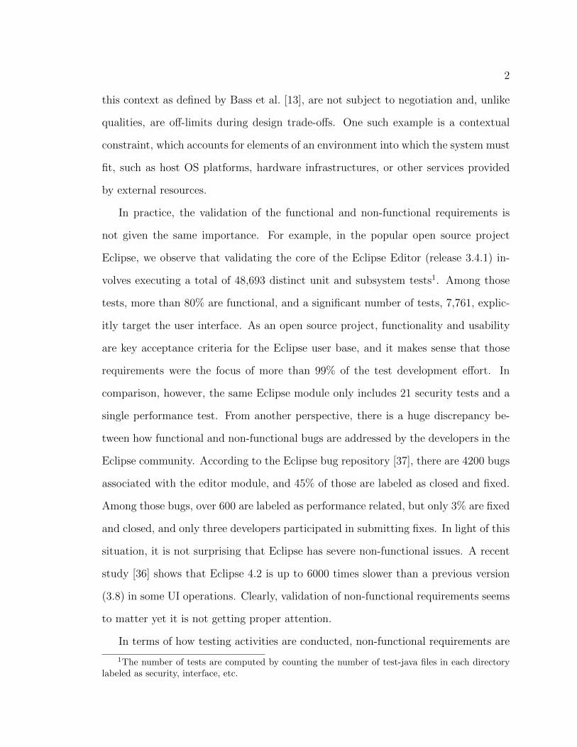
In practice, the validation of the functional and non-functional requirements is

not given the same importance. For example, in the popular open source project

Eclipse, we observe that validating the core of the Eclipse Editor (release 3.4.1) in-

volves executing a total of 48,693 distinct unit and subsystem tests1. Among those

tests, more than 80% are functional, and a significant number of tests, 7,761, explic-

itly target the user interface. As an open source project, functionality and usability

are key acceptance criteria for the Eclipse user base, and it makes sense that those

requirements were the focus of more than 99% of the test development effort. In

comparison, however, the same Eclipse module only includes 21 security tests and a

single performance test. From another perspective, there is a huge discrepancy be-

tween how functional and non-functional bugs are addressed by the developers in the

Eclipse community. According to the Eclipse bug repository [37], there are 4200 bugs

associated with the editor module, and 45% of those are labeled as closed and fixed.

Among those bugs, over 600 are labeled as performance related, but only 3% are fixed

and closed, and only three developers participated in submitting fixes. In light of this

situation, it is not surprising that Eclipse has severe non-functional issues. A recent

study [36] shows that Eclipse 4.2 is up to 6000 times slower than a previous version

(3.8) in some UI operations. Clearly, validation of non-functional requirements seems

to matter yet it is not getting proper attention.

In terms of how testing activities are conducted, non-functional requirements are

1The number of tests are computed by counting the number of test-java files in each directorylabeled as security, interface, etc.

3

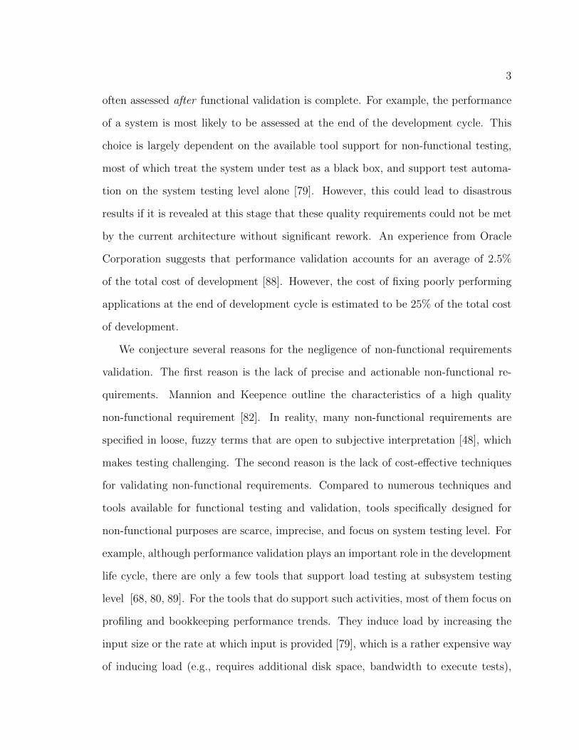
often assessed after functional validation is complete. For example, the performance

of a system is most likely to be assessed at the end of the development cycle. This

choice is largely dependent on the available tool support for non-functional testing,

most of which treat the system under test as a black box, and support test automa-

tion on the system testing level alone [79]. However, this could lead to disastrous

results if it is revealed at this stage that these quality requirements could not be met

by the current architecture without significant rework. An experience from Oracle

Corporation suggests that performance validation accounts for an average of 2.5%

of the total cost of development [88]. However, the cost of fixing poorly performing

applications at the end of development cycle is estimated to be 25% of the total cost

of development.

We conjecture several reasons for the negligence of non-functional requirements

validation. The first reason is the lack of precise and actionable non-functional re-

quirements. Mannion and Keepence outline the characteristics of a high quality

non-functional requirement [82]. In reality, many non-functional requirements are

specified in loose, fuzzy terms that are open to subjective interpretation [48], which

makes testing challenging. The second reason is the lack of cost-effective techniques

for validating non-functional requirements. Compared to numerous techniques and

tools available for functional testing and validation, tools specifically designed for

non-functional purposes are scarce, imprecise, and focus on system testing level. For

example, although performance validation plays an important role in the development

life cycle, there are only a few tools that support load testing at subsystem testing

level [68, 80, 89]. For the tools that do support such activities, most of them focus on

profiling and bookkeeping performance trends. They induce load by increasing the

input size or the rate at which input is provided [79], which is a rather expensive way

of inducing load (e.g., requires additional disk space, bandwidth to execute tests),

4

and may lead to negligence of real performance faults.

In this dissertation we focus on investigating strategies for improving the cost ef-

fectiveness of non-functional validation techniques. We reduce the cost of conducting

non-functional validation by developing techniques that automatically generate test

suites for specific non-functional requirements, and by transforming existing tests into

new tests that add non-functional capabilities to the validation process. We improve

the effectiveness of the techniques by using program analysis to exhaustively tra-

verse program execution paths, searching for instances of violations of non-functional

requirements and producing counter examples (test cases) that allow developers to

easily recreate the failing scenarios.

These techniques can be viewed as complementary to the efforts that aim at

improving the quality of non-functional requirements. If such requirements are avail-

able, our techniques facilitate their validation. If non-functional requirements are not

available, the proposed techniques can still be used to expose worst or near worst

case scenarios of non-functional properties, which could in turn help to develop more

accurate set of non-functional requirements [48, 133].

More specifically, we have targeted two aspects of non-functional testing. For

non-functional requirements defined as qualities of a system, we targeted validation

of performance properties. We improve cost-effectiveness of performance validation by

automatically generating load tests that focus on smart input value selection to expose

worst or near worst case performance scenarios. For non-functional requirements

defined as constraints on a system, we targeted contextual constraints on noisy and

unreliable external resources with which a software system must interact. One way to

improve the robustness of software that interacts with those external resources is to

use exception handling constructs. In practice, however, the code handling exceptions

is not only difficult to implement [95] but also challenging to validate [45, 109, 117].

5

We improve the cost effectiveness of such validation by amplifying existing tests to

exhaustively test every possible execution pattern in which exceptions can be raised,

and produce scenarios in which the exception handling code does not perform as

expected. In the following sections we will discuss each approach in detail.

1.2 Non-functional Requirement Validation: Load

Testing

Load tests aim to validate whether a system’s performance (e.g., response time, re-

source utilization) is acceptable under production, projected, or extreme loads. Con-

sider, for example, an SQL server that accepts queries specified in the standard query

language to create, delete, or update tables in a database. Functional tests would

validate whether a query results in appropriate database changes. Load tests, how-

ever, would be required to assess whether, for example, for a given set of queries the

server responds within an expected time.

Existing approaches to generate load tests induce load by increasing the input

size (e.g., a larger query or number of queries) or the rate at which input is provided

(e.g., more query requests per unit of time)[79]. Consider again the SQL server.

Given a set of tester supplied queries, a load testing tool might replicate the queries,

send them to the SQL server at certain intervals, and measure the response time.

When the measured response times differ from the user’s expectation, which might

be expressed as some upper bound determined by the size or complexity of the queries

or underlying database, a performance fault is said to be detected.

Current approaches to load testing suffer from four limitations. First, their cost

effectiveness is highly dependent on the particular values that are used yet there is

no support for choosing those values. For example, in the context of an SQL server

6

we studied, a simple selection query operating on a predefined database can have

response times that vary by an order of magnitude depending on the specific values

in the select statements. Clearly, a poor choice of values could lead to underestimating

system response time thereby missing an opportunity to detect a performance fault.

Second, increasing the input size may be a costly means to load a system. For

example, in the context of a compression application that we studied, we found that

to increase the response time of the application by 30 seconds one could use a 75MB

input file filled with random values or a 10MB input file if the inputs are chosen care-

fully. This is particularly problematic if increasing the input size requires additional

expensive resources in order execute the test (e.g., additional disk space, bandwidth).

Third, increasing the input size may just force the system to perform more of the

same computation. In the worst case, this would fail to reveal performance faults and,

if a fault is detected, then further scaling is likely to repeatedly reveal the same fault.

In functional testing, diversity in the test suite is desirable to achieve greater coverage

of the system behavior. Load suites that cover behaviors with different performance

characteristics are not a focus of current tools and techniques.

Finally, while most load testing focuses on response time or system throughput,

there are many other resource consumption measures that are of interest to develop-

ers. For example, mobile device platforms place a limit on the maximum amount of

memory or energy that an application can use.

We introduced an approach (Chapter 3) for the automated generation of load test

suites that starts addressing these limitations. It generates load test suites that (a)

induce load by using carefully selected input values instead of just increasing input

size, (b) expose diversity of resource consuming program behavior, and (c) target a

range of consumption measures.

Our white box approach leverages recent advances in symbolic execution to pro-

7

vide smart value selection and diversity in test input generation. However, due to its

exhaustive nature and inherent path explosion problem [73], plain exhaustive sym-

bolic execution cannot scale beyond very small programs. To improve scalability

we developed a search strategy that is directed towards program paths that con-

sume more resources. Our approach is directed and incremental in exploring possible

program paths. The approach is directed by a specified resource consumption mea-

sure to search for inputs of a given size or structure that maximize consumption of

that resource (e.g., memory, execution time). The approach is incremental in that

it considers program paths in phases. Within each phase it performs an exhaustive

exploration of program paths. At the end of each phase, the paths are grouped based

on similarity, and the most promising path from each group, relative to the consump-

tion measure, is selected to explore in the next phase. We implemented the approach

in the Symbolic Path Finder framework [65] and assessed its effectiveness on three

artifacts. The results indicate that the proposed approach can produce suites that

induce response times several times greater than random input selection and can

scale to millions of inputs, increase memory consumption between 20% and 400%

when compared with standard benchmarks, and expose different ways to induce high

consumption of resources.

If improving on symbolic execution alone would not lead to desirable scalabil-

ity suitable for load testing, we reconstruct the analysis compositionally, following a

‘divide-and-conquer’ strategy. We have proposed a compositional approach to gener-

ate load tests (Chapter 4). The approach builds on the aforementioned technique to

collect the program paths that would lead to an effective load test suite for each system

component. The collected paths constitute a performance summary for each compo-

nent. The approach is compositional in that it analyzes the components’ summaries

and their connections to identify compatible paths, as defined by their constraints,

8

which can be solved to generate load tests for the whole system. Key to this process

is how path constraints across components must be weighted and relaxed in order

to derive test inputs for the whole system while ensuring that the most significant

constraints, in terms of inducing load, are enforced. We have implemented the ap-

proach by using our previous load generation approach as a subroutine for collecting

performance summaries. An evaluation on a group of Unix pipeline artifacts and

one XML pipeline shows that the compositional approach achieves scalability beyond

that of the previous technique, and has an effectiveness gain of 288% over Random

when given the same time to generate tests. In its current form, the compositional

approach is fully automated to handle software that follows the pipeline architecture.

We have also presented an extension of the approach that enables handling of Java

programs, in which each component is a Java method. We have presented a set of new

algorithms to handle the added challenges, such as more complex program structures

and more sophisticated summary composition strategies. We showed the viability of

the extended approach through a series of examples.

1.3 Non-functional Requirement Validation: Ex-

ception Handling

Modern software does not execute in isolation. It interacts with external resources

that can be noisy and unreliable, and exhibit transient and unpredictable failures

[98]. One way to improve software robustness in such a context is to use exception

handling constructs. In practice, however, the code handling exceptions is not only

difficult to implement [95] but also challenging to validate (e.g., [45, 109, 117]).

We conjecture that the validation challenge is particularly relevant when deal-

ing with systems that must interact with external resources that can be noisy and

9

unreliable, and exhibit transient and unpredictable failures [98]. Consider, for ex-

ample, an exception handling construct to check for the end of a sequential input

stream. The reliability of the stream is rarely in doubt, the end of the file is a cer-

tainty, and standard testing frameworks provide mocking support for streams. In

contrast, an exception handling construct interacting with noisy and often unreliable

localization, communication, and sensor services, cannot make such simplifying as-

sumptions, requiring more complex and hence harder to validate implementations. A

standard testing framework, which only supports simple ways of mocking the API

calls that invoke those services, cannot accurately model the noisy nature of the ex-

ternal resources, and misses the faults that can only be triggered by specific patterns

of exceptions.

To assess the severity of the problem, we conducted a study on fault repositories

of eight popular Android applications. The study provides quantifiable evidence of

the commonality of faults associated with exception handling code constructs, and

more specifically with those related to handling external resources with unpredictable

performance that cannot be controlled through standard input manipulation. The re-

sults show that 22% of the confirmed and fixed bugs have to do with poor exceptional

handling code, and that 12% correspond to interactions with four external resources

we deem most relevant to the problem (Section 5.1).

We then presented an exhaustive white box approach to support the detection of

such faults (Section 5.3). Our approach is simple, scalable, and effective in practice

when combined with a test suite that invokes the resources of interest. The approach

is white box in that it first instruments the target program so that the results of calls

to external resources of interest can be mocked at will to return exceptions. Then,

existing test cases are systematically amplified by re-executing them on the instru-

mented program under various mocked patterns to explore the space of exceptional

10

behavior. The approach exhaustively tests all patterns, looking for the ones that are

effective in exposing faults. When a fault is revealed, the mocking pattern applied

with the test serves as an explanation of the failure induced by the external resource.

To control the number of amplified tests the approach prunes tests with duplicate

calls and call-outcomes to the external resources, and bounds the number of calls

that define the space of exceptional behavior explored.

The approach is built on two assumptions. First, it builds on the small scope

hypothesis [64], often used by techniques that systematically explore a state space,

which advocates for exhaustively exploring the program space up to a certain bound.

The underlying premise is that many faults can be exposed by performing a bounded

number of program operations, and that by doing so exhaustively no corner cases (test

cases that expose faults in extreme situations, such as extreme values for the input

parameters) are missed. Several studies and techniques have shown this approach to

be effective (e.g., [18, 29, 32]) and we build on those in this work. In our approach,

the bound corresponds to the length of the mocked patterns. Second, we assume that

the program under test has enough tests cases to provide coverage of the invocations

to the resources of interest. The increasing number and maturity of automated test

case generation techniques and tools support this assumption. If this assumption

holds, then the approach can automatically and effectively amplify the exposure of

code handling exceptional behavior.

1.4 Dissertation Statement

In the dissertation we explore the following research statement:

Bounded exhaustive white box testing techniques can cost effectively validate non-

11

functional requirements.

We have investigated this statement from two perspectives. For non-functional

requirements defined as qualities of a system, we targeted load testing for the purpose

of performance validation. We present a load test suite generation approach by using

symbolic execution to exhaustively traverse program execution paths and produce test

cases for the ones that expose worst case resource consumption scenarios. For non-

functional requirements defined as constraints on a system, we present an approach for

validating contextual constraints that are imposed by external resources with which

a software interacts. The approach amplifies existing tests in an exhaustive manner

to validate exception handling constructs that are used to handle such constraints.

Combined, the two proposed techniques complement the field of automated software

testing by providing exhaustive support for non-functional validation.

1.5 Contributions of this Research

In this dissertation, we have developed a set of exhaustive white box testing techniques

to support automatic validation of non-functional requirements. The contributions

of this work are three-fold:

1. Symbolic Load Generation. For performance validation we have developed

a technique for automated generation of load test suites with support for pre-

cise input value selection that is built on state-of-the-art symbolic execution

techniques, and equipped with a directed incremental search strategy to tai-

lor the special needs of load generation. An assessment of the approach shows

it generates test suites that induce program response times and memory con-

sumption several times worse than the compared alternatives, it scales to large

12

and complex inputs, and it exposes a diversity of resource consuming program

behavior [137] (see Chapter 3 for details).

2. Compositional Load Generation. To further improve on the scalability

of the symbolic load generation technique, we developed a compositional tech-

nique for automated generation of load tests for more complex software systems.

The technique is compositional in that it analyzes each software components’

performance in isolation, then generates load tests for the whole system by

accumulating and stitching each performance summary. An evaluation of the

technique on software pipelines shows that it achieves scalability beyond that of

the symbolic load generation technique, and has an effectiveness gain of 288%

over random when given the same time to generate tests [138]. We further

generalize the technique to load test generation for Java programs, provide a

conceptual implementation sketch, and illustrate its application through a series

of examples (see Chapter 4 for details).

3. Exception Handling Validation. For exception handling validation, we first

assessed the magnitude of the problem by conducting a study on fault reposito-

ries of eight popular Android applications. We then developed a technique that

systematically amplifies existing tests to validate exception handling code in an

exhaustive manner. Our assessment of the technique indicates that it can be

fully automated, is powerful enough to detect 67% of the faults reported in the

bug reports of this kind, and is precise enough that 78% of the detected anoma-

lies correspond to faults fixed by the developers. The technique outperforms a

state of the art approach [117] in precision and recall. In addition, the feed-

back from developers and the preliminary case study illustrate the techniques

potential to assist developers [136] (see Chapter 5 for details).

13

1.6 Outline of Dissertation

The remainder of this dissertation is organized as follows: Chapter 2 discusses related

work and describes the fundamental concepts that are relevant to the techniques pre-

sented in the thesis, such as symbolic execution, performance testing, and techniques

for testing of exception handling code. Chapter 3 presents the load test generation

technique for standalone programs. In Chapter 4, we introduce the technique for

compositional load generation for software pipelines as well as Java programs. In

Chapter 5, we present the technique for amplifying tests to validate exception han-

dling code. Finally, in Chapter 6, we provide the overall conclusions for this work,

summarize the merit and impact, and present ideas for improvements and future

research directions.

14

Chapter 2

Background & Related Work

In this chapter, we identify key pieces of work that are related to our approaches in

the two proposed areas. For our work on load testing, we begin with background

information on symbolic execution, a fundamental technique used by our technique.

We then discuss recent improvements to symbolic execution and how we benefited

from those improvements. We also identify other techniques that aim at load test gen-

eration or performance characterization in general, and discuss how they are related

to ours. For our work on validating exception handling code, we identify two areas of

related work: mining exception handling specifications and exception handling code

coverage representations, and discuss how they are related to our technique.

2.1 Symbolic Execution

Symbolic execution [73] simulates the execution of a program using symbolic values in-

stead of actual values as inputs. During symbolic execution, when a program variable

is read, its corresponding symbolic value is loaded. Memory locations are updated

with symbolic values when they are written during symbolic execution.

A symbolic execution tree characterizes the execution paths generated during sym-

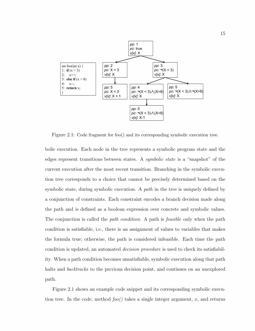
15

int foo(int x) { 1: if (x < 3) 2: x++; 3: else if (x > 8) 4: x--; 5: return x; }

pp: 1 pc: true v[x]: X

pp: 2 pc: X < 3 v[x]: X

pp: 3 pc: ¬(X < 3) v[x]: X

pp: 5 pc: X < 3 v[x]: X + 1

pp: 4 pc: ¬(X < 3)∧(X>8) v[x]: X

pp: 5 pc: ¬(X < 3)∧¬(X>8) v[x]: X

pp: 5 pc: ¬(X < 3)∧(X>8) v[x]: X-1

Figure 2.1: Code fragment for foo() and its corresponding symbolic execution tree.

bolic execution. Each node in the tree represents a symbolic program state and the

edges represent transitions between states. A symbolic state is a “snapshot” of the

current execution after the most recent transition. Branching in the symbolic execu-

tion tree corresponds to a choice that cannot be precisely determined based on the

symbolic state, during symbolic execution. A path in the tree is uniquely defined by

a conjunction of constraints. Each constraint encodes a branch decision made along

the path and is defined as a boolean expression over concrete and symbolic values.

The conjunction is called the path condition. A path is feasible only when the path

condition is satisfiable, i.e., there is an assignment of values to variables that makes

the formula true; otherwise, the path is considered infeasible. Each time the path

condition is updated, an automated decision procedure is used to check its satisfiabil-

ity. When a path condition becomes unsatisfiable, symbolic execution along that path

halts and backtracks to the previous decision point, and continues on an unexplored

path.

Figure 2.1 shows an example code snippet and its corresponding symbolic execu-

tion tree. In the code, method foo() takes a single integer argument, x, and returns

16

an integer value. It has two branching points (Line 1 and Line 3) and three feasible

paths (shown on the right).

Each symbolic state is defined as a triple, (pp, pc, v). The program position, pp,

denotes the next statement to be executed. The path condition, pc, is a conjunction

of the constraints on the symbolic variables along the current execution path. The

symbolic value map, v, is a map from memory locations of the program variables to

symbolic expressions representing their current values. For example, in Figure 2.1,

the last state of the middle path on the symbolic execution tree (the bottom box)

includes pp at Line 5, a pc: ¬(X < 3)∧ (X > 8), and one symbolic expression X − 1

for the variable x.

To illustrate how symbolic execution works, again consider the example in Fig-

ure 2.1. When foo() is invoked, the path condition is initialized to true, and the

symbolic value map for variable x contains the symbolic value X (we use capital let-

ters to indicate symbolic values). At Line 1, symbolic execution branches: (1) when

X < 3, the value of x is incremented at Line 2, and the value X + 1 is returned

at Line 5; (2) when ¬(X < 3), the execution moves to Line 3 and branches again:

(1) when X > 8, the value of x is decremented at Line 4, and the value X − 1 is

returned at Line 5; (2) when ¬(X > 8) the execution moves to Line 5 and returns the

original value X. Symbolic execution on this code generates a total of three paths,

as illustrated on the right in Figure 2.1.

The simplicity of this example belies the true complexity of performing symbolic

execution on real programs. In the next sections, we will describe some of the more

challenging aspects of performing symbolic execution in a realistic environment, such

as handling complex inputs, scaling up to complex programs, and its application to

automatic test generation.

The work in Chapters 3 and 4 are built on symbolic execution techniques, but

17

are unique in their application to load testing, which requires the development of

different search heuristics and exposes different tradeoffs and scalability issues.

2.1.1 Generalized Symbolic Execution

Symbolic execution was first introduced as a technique for generating test inputs on

scalar inputs. In 1976, King presented an interactive system that provides symbolic

execution for programs written in a PL/I style language for testing and debugging [73].

In recent years, thanks to the substantial advances in raw computation power and

constraint solving technology, symbolic execution has regained its popularity as a

promising technology for test generation research [91].

The rise of object-oriented programing languages in the 90s makes symbolic ex-

ecution of software written in such languages more challenging: 1) OO programs

frequently use dynamically allocated data, such as trees, linked lists, or arrays of un-

specified lengths, as inputs. Declaring these types of inputs as symbolic variables is

challenging because it would require modeling them in the symbolic heap and updat-

ing their structures as the analysis continues. 2) For symbolic execution techniques

that correctly model the symbolic heap, the number of possible outcomes for updat-

ing a symbolic data structure (such as an symbolic tree) in the heap is prohibitively

large, making the technique non-scalable even for tiny examples. 3) A program may

use complex library calls in it computation, resulting in non-linear constraints (e.g.,

strings and high-order mathematical constraints) that can not be solved by tradi-

tional decision procedures; or it may make references to native libraries, for which

code may not be available to analyze at source code level.

For programs whose inputs are heap-allocated data structures, Khurshid et al.

proposed lazy initialization [72]. It starts execution of the program on inputs with

uninitialized fields and assigns values to these fields lazily, i.e., when they are first

18

accessed during symbolic execution of the code. It nondeterministically initializes the

field to null, to a reference of a new object with uninitialized fields, or to a reference

of an object created during a prior field initialization. The technique branches on

these choices, which effectively systematically treats all aliasing possibilities. This

approach eliminates the need to specify an a priori bound on the number of input

objects, which is generally unknown.

To solve the problem of poor scalability caused by the introduction of sym-

bolic heap data, Visser et al. proposed state abstraction and subsumption tech-

niques [4, 122]. In this line of work, the authors first described abstraction mapping,

an approach that maps heap objects in the symbolic state to a simplified version

(e.g., representing a chain of nodes in a linked list with one summarizing node). The

authors then present subsumption, a method for examining whether a symbolic state

is subsumed by another symbolic state. Subsumption is used to determine when a

symbolic state is revisited, in which case the model checker backtracks, thus prun-

ing the state space. In this process, abstraction is used to increase chances of state

matching. This effectively explores an under-approximation of program behaviors,

but has proved to be effective in generating tests for programs that take container

objects as inputs, e.g., binary search trees, arrays.

For symbolic execution involving strings, several approaches have proposed using

string solvers [47, 104]. String constraints are collected in conjunction with con-

straints on scalar variables, and both scalar / string decision procedures are used

in satisfiability checks. For other types of complex constraints and native library

calls, Pasareanu et al. proposed to solve the problem with uninterpreted functions

and mixed concrete-symbolic solving [90]. This technique splits the generated path

conditions into two parts: 1) constraints that can be solved by a decision procedure,

and 2) complex non-linear constraints with uninterpreted functions to represent ex-

19

ternal library calls. Simpler constraints are solved first and the solutions (concrete

values) are used to simplify the complex constraints; the resulting path conditions

are checked again for satisfiability.

Our load test generation technique takes advantage of some of these advances. Our

technique support arrays of unspecific length through lazy initialization, and string

operations through the use of string decision procedures. Furthermore, we extended

the support of external library calls to file system operations through modeling of a

symbolic file system, details of which are discussed in Chapter 4.

2.1.2 Dynamic Symbolic Execution

Dynamic symbolic execution aims to improve performance of symbolic execution by

combining concrete and symbolic execution, essentially bounding the scope of what

is treated as symbolic. First introduced by Godefroid et al. in DART (Directed

Automated Random Testing) [51], the idea is to perform a concrete execution on

random inputs and at the same time to collect the path constraints along the executed

path. These path constraints are then used to compute new inputs that drive the

program along alternative paths. More specifically, one can negate one constraint at a

branch point to guide the test generation process towards executing the other branch.

A constraint solver is called to solve the path constraints and to obtain the test inputs.

The program is executed on these new inputs, constraints are collected along the new

program path and the process is repeated until all the execution paths are covered

or until the desired test coverage is achieved. For example, for the code fragment in

Figure 2.1, after exploring the path: ¬(X < 3)∧(X > 8), dynamic symbolic execution

can negate the branch at Line 3 to explore a new path: ¬(X < 3) ∧ ¬(X > 8).

Whenever symbolic execution gets stuck, dynamic symbolic execution uses con-

crete values to simplify the constraints, which leads to improved scalability, but loses

20

completeness. Note that both dynamic symbolic execution and generalized sym-

bolic execution aim to help traditional symbolic execution in certain situations, e.g.,

when there are no available decision procedures or in the presence of native calls,

however they use different approaches to achieve this goal. Dynamic symbolic exe-

cution uses values from concrete runs to handle situations that decision procedures

can not handle, while generalized symbolic execution uses concrete solutions of the

solvable constraints in the current path condition to simplify the overall complexity.

Implementation-wise, dynamic symbolic execution explores new paths by negating

constraints on the current path, which is mostly implemented by code instrumen-

tation, while generalized symbolic execution uses state-space search to explore new

paths, which is mostly implemented on top of a state-space exploration framework

(usually a model checker). Both techniques are implemented through several tools,

which explore different tradeoffs between scalability and completeness. We will dis-

cuss those tools in the next section.

2.1.3 Using Symbolic Execution for Automatic Test Gener-

ation

One direct application of symbolic execution is the automated generation of test cases

that reach certain statements, achieve high degree of coverage, or expose certain bugs.

Symbolic execution is well suited for the task, because the path condition to reach a

statement in the code when solved, gives exactly the input to reach the statement.

There is a large body of work in this research direction, we review some of the most

representative ones below.

Symbolic Path Finder. Pasareanu et al. proposed Symbolic Path Finder (SPF) [92],

a symbolic execution engine built on the model checking tool called Java Path Finder

21

(JPF) [65] to enable symbolic execution on Java programs. It is built on generalized

symbolic execution, the technique presented in Section 2.1.1. SPF implements a non-

standard interpreter of Java bytecode using a modified JPF Java Virtual Machine to

enable symbolic execution. SPF stores symbolic information in attributes associated

with the JPF program states. The underlying model checker core provides many

benefits to the symbolic execution engine, such as built-in state space exploration

capabilities, a variety of heuristic search strategies, as well as partial order and sym-

metry reductions. In addition, it handles complex input data structures and arrays

via lazy initialization, and implements state abstraction and subsumption checks. In

addition, SPF addresses the issue of scalability with mixed concrete/symbolic exe-

cution [92]. The idea is to use concrete system-level simulation runs to determine

constraints on the inputs to the units within the system. The constraints are then

used to specify pre-conditions for symbolic execution of the units. SPF is used to

analyze prototype NASA flight software components and helps to discover several

bugs [92, 90].

DART. Proposed by Godefroid et al., DART [51] is the first among the line of work

that use dynamic symbolic execution to generate tests (Section 2.1.2). This approach

is alternatively named “concolic testing” - aiming to blend concrete and symbolic

executions to improve the scalability of traditional symbolic execution approaches.

DART, which generates tests for C programs, starts to execute a program with ran-

dom concrete inputs, gathers symbolic constraints on inputs along the execution, and

then systematically or heuristically negates each constraint in order to steer the next

execution towards an alternative path. DART is used to generate tests for applica-

tions ranging from 300 to 30,000 lines of code, and detected several bugs. Note that

SPF also improves scalability by mixing concrete and symbolic executions, but with

22

a different methodology. DART performs concrete execution on whole paths and uses

the results to steer towards alternative paths, while SPF interleaves concrete and sym-

bolic executions and uses concrete execution to setup the environment for symbolic

execution [92]. In addition, as discussed in Section 2.1.2, both techniques use concrete

execution results to handle native library calls, but with different methodologies as

well.

CUTE. CUTE [102] is another concolic execution technique for C programs that

improves on DART by providing support for heap-allocated dynamic data structures

as inputs. The key idea is to represent all inputs with a logical input map, and then

collect two separate kinds of constraints, scalar constraints and pointer constraints,

as symbolic execution proceeds. The pointer constraints are collected approximately

— the only types of pointer constraints allowed are aliasing and null pointers. All

other properties of pointers, such as boundary checks and offsets, are ignored. With

this improvement, CUTE enables test generation for dynamic data structures such

as trees and linked lists.

EXE and KLEE. EXE [24] is a symbolic execution technique designed for systems

code in C language, such as device drivers OS kernels. The unique feature in EXE

is that it models memory with bit-level accuracy, which is necessary for handling

systems code, which often treats memory as raw bytes and casts them in a variety

of ways. EXE also uses a custom decision procedure, STP [46], to speedup the

solving process. KLEE [23] is a redesign of EXE built on top of the LLVM [74]

compiler infrastructure. This design, along with several improvements in storing and

retrieving program states, provides further scalability gains to the technique. Another

improvement of KLEE is the ability to handle file systems and network operations. It

provides symbolic models of these external libraries and supports symbolic execution

23

on these operations. However, neither EXE nor KLEE supports non-linear arithmetic

operations, in which case, concrete values are used instead. In terms of scalability,

EXE is used to generate tests for applications such as network protocols and Linux

kernel modules (e.g., mount), ranging from a few hundred to 2K lines of source code.

It is shown to successfully generate inputs that detect bugs in these applications.

On the other hand, KLEE pushes scalability to a higher level by detecting bugs on

applications of 2K-8K lines of code.

Pex. Pex [119], developed by Microsoft Research, is another concolic execution tool

to generate test inputs for the .NET platform. It has been released as a plugin for

Microsoft Visual Studio and used daily by several groups within Microsoft. Pex uses

the Z3 solver [33] as the underlying decision procedure, and uses approximations

to handle types of constraints for which Z3 has not supported, such as strings and

floating point arithmetic. There have been a number of extensions to Pex, such as

support for heap-allocated data [118], which allows test generation for data structures

such as trees and linked lists, and new search strategies [127], which use the fitness

function in genetic algorithms to guide search.

SAGE. Godefroid et al. proposed a technique called “SAGE: white-box fuzzing” [50],

which targets programs whose inputs are determined by some context free grammars,

such as compilers and interpreters. The technique abstracts the concrete input syntax

with symbolic grammars, where some original tokens are replaced with symbolic con-

stants. This operation reduces the set of input strings that must be enumerated. As

a result, the inputs generated by this technique can easily pass the front-end (lexers

and parsers) of the software under test, and reach deeper stages of execution, increas-

ing its chance of catching bugs. The technique has been used to validate applications

such as a JavaScript interpreter of Internet Explorer 7. In essence, this technique

24

can be viewed as another attempt to combine symbolic and concrete executions. It

is unique in that it uses symbolic grammars to reduce the set of input strings for

software systems. Since then, similar ideas have been adopted by other researchers

to enable validation of applications such as logical formula solvers [81], server-side

application architectures [63], web pages [10, 132], and database applications [39].

Our load generation technique, SLG (Chapter 3), is built on top of SPF, and takes

advantages of its built-in features, such as support for heap-allocated data, support

for string solvers, and mixed concrete / symbolic execution. Furthermore, we have

extended SPF to support symbolic file systems, a design that was inspired by the

KLEE tool [23].

2.1.4 Search Heuristics in Symbolic Execution

A typical symbolic execution framework often provides a rich set of search heuristics.

A search heuristic essentially determines the priority of target branches to explore

next. In the extreme, full program behaviors can be explored via an exhaustive

strategy. Within this category, there are many well-known search strategies such

as breadth-first (BFS) and depth-first search (DFS) strategies. However, each such

strategy is biased towards particular branches. While breadth-first search favors

initial branches in the program paths, the depth-first search favors final branches.

Most symbolic execution techniques support a mixture of the above heuristics.

DART and CUTE use DFS. EXE also uses DFS as its default strategy, but provides

an alternative strategy, which is a mixture of best-first (Best-FS) and DFS [23]. The

strategy works as follows: the search starts with DFS, after four branches, it uses

heuristics to evaluate all forked paths, picks the one with the best progress (in terms

of coverage) to continue first, then does another four steps of DFS. The goal of this

strategy is to provide some global perspective occasionally, in order to prevent DFS

25

from sinking in a local subtree. SPF also includes strategies like BFS, DFS, and

Random, along with other legacy heuristics (such as Best-FS and BEAM) passed

down from the model checker JPF [56].

One interesting work by Xie et al. introduces the concept of fitness function from

genetic algorithms to the area of concolic execution [127]. The proposed technique,

which is termed “fitness function guided search”, assigns fitness values to each ex-

plored path. A fitness function measures how close an explored path is in achieving

a test target coverage. A fitness gain is also measured for each explored branch: a

higher fitness gain is given to a branch if flipping it in the past helped achieve better

fitness values. Then during path exploration, the technique would prefer to flip a

branch with a higher fitness gain in a previously explored path with a better fitness

value. The goal of this technique is to identify high coverage paths quickly, without

getting stuck in a large space of less valuable paths.

For our load test generation technique SLG, we developed unique search strategies

specifically tailored to our needs. Rather than performing a complete symbolic exe-

cution, it performs an incremental symbolic execution to more quickly discard paths

that do not seem promising, and directs the search towards paths that are distinct

yet likely to induce high load as defined by a performance measure. We will explain

the details of this strategy in Chapter 3.

2.1.5 Memoization in Symbolic Execution

Memoization is a technique for giving functions a memory of previously computed

values [83]. Memoization allows a function to cache values that have already been

calculated, and when invoked under the same preconditions, to return the same value

from a cache rather than recomputing each time. Memoization explores the time-

space tradeoff, and can provide significant performance gains for programs that con-

26

tain many computation-intensive calls.

The concept of memoization has also been applied to program analysis techniques,

such as software model checking and symbolic execution. Analogous to classical

memoization, the results of previous analysis on functions are cached, and then reused

accordingly to save time. For example, Lauterburg et al. proposed ISSE (Incremental

State-Space Exploration) [75], a model checking technique that stores the state space

graph during a full model checking of a program, and then reduces the time necessary

for model checking of an evolved version of the program by avoiding the execution of

some transitions and related computations that are not necessary. We now discuss

the application of memoization in symbolic execution.

Memoization at the functional level. Recent work [3, 49] proposes composi-

tional reasoning as a means of scaling up symbolic execution. Godefroid et al. pro-

posed the SMART technique [49], which is intended to improve the scalability of

DART. The idea is to reuse summaries of individual functions computed from pre-

vious analysis. A summary consists of pre-conditions on the functions inputs and

post-conditions on the functions output; they are computed “top down”, to take into

account the proper calling context of the function under analysis. If f() calls g(),

one can summarize g() the first time it is explored, and reuse g()’s summary when

analyzing f() later on. Thus, each method is analyzed separately and the overall

number of analyzed paths is smaller than in the case where the system is analyzed

as a whole. Anand et al. extend the compositional analysis with a demand-driven

approach [3], which avoids computing summaries unnecessarily, i.e., summaries that

will never be used. Instead, summaries are computed as-needed on the fly.

Memoization on full paths. Application of symbolic execution often requires

several successive runs on largely similar programs, e.g., running it once to check a

27

program to find a bug, fixing the bug, and running it again to check the modified

program. Similar usage scenarios can also be observed in regression testing and

continuous testing [97]. Yang et al. proposed Memoise, a technique as a means of

scaling up symbolic execution in this type of usage scenarios [130]. It uses a trie-based

data structure to store the key elements of a run of symbolic execution, and it reuses

this data to speedup successive runs of symbolic execution on a new version of the

program. The savings are achieved in a regression analysis setting, in which multiple

program versions are available. However, the exact savings are hard to predict, as

they depend on the location of the change, and may vary quite a lot between different

changes.

Our technique of compositional load generation is inspired by previous work on

compositional symbolic execution, but with different goals and mechanisms. For

example, in resolving inconsistencies through constraint relaxation, our technique

resorts to the performance tags associated with the path constraints in order to max-

imize the load that the generated test will induce. To the best of our knowledge,

our work is the first one to utilize compositional symbolic execution to generate non-

functional tests.

2.2 Automated Techniques for Load Testing

In this section we first present an extensive review of related work on automated

techniques for load test generation. Techniques in this area can be roughly catego-

rized into two categories: black-box techniques, which treat the system under test

as a black box; and white-box techniques, which have access to the source code of

the system under test. We will review techniques in both categories, identify their

potential and drawbacks, and discuss how our techniques are related to those. In

28

addition, there is a large body of work on automatic / semi-automatic identification

of bottlenecks (or performance bugs) in the source code. Although our current work

focuses on generation of load tests, our future goal on load testing includes identifying

bottlenecks as well. Therefore, we will present a review on this line of work as well.

2.2.1 Generating Load Tests

Black-box Techniques. There is a large number of tools for supporting load test-

ing activities [79], some of which offer capabilities to define an input specification

(e.g., input ranges, recorded input session values) and to use those specifications to

generate load tests [108]. For example, a popular tool like Silk [108] provides a user

interface and wizards to define a typical user profile and scenario, manipulate the

number of virtual users to load a system, and monitor a vast set of resources to mea-

sure the impact of different configurations. Clearly, more accurate and richer user

and scenario specifications could yield more powerful load tests. Support for identi-

fying the input values corresponding to the most load-effective profiles and scenarios,

however, is very limited.

A common trait among these tools is that they provide limited support for select-

ing load inducing inputs as they all treat the program as a black box. The program

is not analyzed to determine what inputs would lead to higher loads, so the effective-

ness of the test suite depends exclusively on the ability of the tester to select values.

Similar trends appear in load testing techniques and processes in general as they use

other sources of information (e.g., user profiles [11], adaptive resource models [14]) to

decide how to induce a given load, but still operating from a black box perspective.

One recent advance in this area is the FORPOST technique proposed by Grechanik

et al. [55]. The technique is novel in that it uses an adaptive, feedback-directed

learning algorithm to learn rules from execution traces of applications, and then uses

29

these rules to select test input data to find performance bottlenecks. It has been

shown to help identifying bottlenecks in two applications: an insurance application,

for which the inputs are customer profiles; and an online pet store, for which the

inputs are URLs selecting different functions in online shopping. When FORPOST

is applied to these applications, it automatically learns rules on the bad inputs (high

loads) such as: a customer should have home/auto discount, or a customer has viewed

more than 16 items, etc. It then uses these rules to derive test inputs, such as customer

profiles that have home/auto discounts, that lead to high workloads. Bottlenecks are

identified by comparing good with bad test cases: a prominent resource consuming

method that occurs in good test cases (high load), but is not invoked or has little

significance in bad test cases (low load), is likely to be a bottleneck. This approach

works well if there exists a large pool of candidate inputs, the variety among candidate

inputs is high, and the properties of the inputs can be expressed by simple rules.

Unlike these black-box techniques, our load test generation technique uses a white-

box approach to generate tests. We view black-box approaches as complementary,

where a hybrid approach may combine the benefits of both approach in a gray-box

performance testing, in which a white-box approach is used to select precise input

values, and a black-box approach is used to learn input rules, which in turn would

help improving scalability of the white-box approach.

White-box Techniques. Until recently, techniques and tools for performance val-

idation or characterization have treated the target program as a black box. One

interesting exception is an approach proposed by Yang et al. [129]. Conceptually, the

approach aims to assign load sensitivity indexes to software modules based on their

potential to allocate memory, and use that information to drive load testing. Our

approach also considers program structure, but a key difference in that, instead of

30

having to come up with static indices, our approach explores the program system-

atically with the support of symbolic execution to identify promising paths that we

later instantiate as tests.

The WISE technique proposed by Burnim et al. proposes to uses symbolic ex-

ecution to identify a worst-case scenario [20]. The technique utilizes full symbolic

execution on small data sizes, and then attempts to generalize the worst case com-

plexity from those small scenarios. This works well when the user can provide a

branch policy indicating which branches or branch sequences should be taken or not

in order to generalize the worst-case from small examples, which requires an extremely

good understanding of the program behavior. The study shows that an ill-defined

branch policy fails to scale even for tiny programs like Mergesort.

Our approach is different in two significant respects. First, our work is designed

to targets scalability specifically. We characterize the components of a system by

performing an incremental symbolic execution favoring the deeper exploration of a

subset of the paths associated with code structures. This removes the requirement for

a user-provided branch policy. For the entire system, we use a compositional approach

to avoid exploring whole program paths and facing path explosion problem. Second,

our goal is to develop a suite of diverse tests, not just identifying the worst-case. This

requires the incorporation of additional mechanisms and criteria to capture distinct

paths that contribute to a diverse test suite, and of a family of performance estimators

that can be associated with program paths.

2.2.2 Identifying Performance Problems

Profiling-based Techniques. The most common way of identifying performance

problems is through profiling of the system under test. Over the years, profiling tools

such as gprof [54] has been used to find bottlenecks related to excessive CPU usage.

31

From the memory consumption perspective, Seward et al. propose Memcheck [103], a

tool that performs memory usage profiling of a subject program. The results of Mem-

check can be used to help identify memory bottlenecks and other types of memory

related errors. Memcheck is built on top of Valgrind [85], a binary instrumentation

framework. It maintains a shadow value for every register and memory location, and

uses these shadow values to store additional information, which enables tracking of

all types of memory operations, such as value initialization, allocation/deallocation,

copying, etc. Although programs instrumented with Memcheck typically run 20-30

times slower than normal, it is claimed to be fast enough to use with large programs

that reach 2 million lines of code.

However, profiling tools often rely on one specific run of the program under test.

Selecting the ‘right’ input that will expose the resource consumption problems be-

comes critical, and in practice often leads to missed performance bugs. In recent

years, several works have been done to alleviate this problem, either by aggregating

information from multiple runs (possibly with order of magnitude difference in input

data sizes), in the hope of providing “cost functions” for the key methods in the

system, or by mining from millions of traces collected on deployed software systems.

Goldsmidth et al. propose an approach that, given a set of loads, executes the

program under those loads, groups code blocks of similar performance, and applies

various fit functions to the resulting data to summarize the complexity [52]. This

approach is applied to various applications such as a data compression program,

a C language parser, and a string matching algorithm, and is able to confirm the

expected performance of the implementation of those classic algorithms. Although the

approach improves dramatically from single run profiling, the user provided workloads

still proves to be critical to the performance of this approach.

Gulwani et al. take a static approach [58]. Their approach instruments a program

32

with counters, uses an invariant generator to compute bounds on these counters, and

composes individual bounds together to estimate the upper bound of loop iterations.

This approach relies on the power of the invariant generator and the user input of

quantitative functions to bound any type of data structures. As a result, this approach

is demonstrated to scale only to small examples up to a hundred lines of code.

Coppa et al. propose a new profiling tool, aprof [28], that further alleviates the

problem of relying user provided workloads. aprof also generates performance curves

of individual methods in terms of their input sizes. However, instead of allowing

users to provide work loads that range orders of magnitude in size, aprof only needs

a few runs under a typical usage scenario. The key insight is that aprof automatically

identifies different sizes of inputs to a specific method by monitoring its read memory

size in each invocation. The approach is evaluated on a few components in the SPEC

CPU2006 benchmarks, and is shown to provide informative plots from single runs on

typical workloads. However, aprof does not consider alternative types of inputs that

are received during runtime, such as data received on-line (e.g., reads from external

devices such as the network, keyboard, or timer). The accuracy of the approach would

be undermined in those situations.

Zaparanuks et al. propose another profiling tool, AlgoProf [133], that attempts

to achieve a similar goal as aprof, but uses different types of metrics. Instead of

using cost metrics such as invocation counts, response times, or instruction counts,

AlgoProf uses a set of metrics that focus on repetitions, i.e., loop counts, recursions,

and data structure access counts. As a result, AlgoProf produces cost functions

that are more focused on the algorithmic complexity. AlgoProf is shown to provide

accurate performance plots for classical data structure algorithms such as trees and

graphs, and is proved useful in uncovering algorithmic inefficiencies. However, it is

not clear whether this type of metrics is as useful in broader types of applications.

33

Han et al. propose StackMine [60], a tool that takes a different approach to avoid

the workload dependent problem. Instead of focusing on a few isolated runs, Stack-

Mine works on millions of stack traces collected on the deployed software systems

(e.g., Microsoft Windows Error Reporting Tool). It uses machine learning algorithms

to mine suspicious traces out of those traces: a sequence of calls appearing a long

time across multiple stacks can be a CPU consumption bug; a sequence of calls wait-

ing long time across multiple stacks can be a wait bug. This technique provides an

alternative approach to performance debugging in the large, if the user can afford to

collect a large amount of stack trace data on deployed products, which is generally

expensive and fragmented.

Our work complements these techniques, because we focus on selecting input

values that lead to worst case performances. We conjecture that the generated input

values can in turn be used to enable a more accurate profiling of the program under

test.

Search-based Techniques. Another thread of related works aim to predict overall

performance of a system at a stage where only performance evaluation of the con-

stituent components are available [1, 12, 107]. This type of information is valuable,

because it can predict performance of systems that are yet to be built, therefore avoid-

ing system architectures that are doomed to lead to bad performance. For example,

Siegmund et al. proposed a technique that can predict program performance based

on selected features in a software product line environment [107]. The proposed tech-

nique models the problem as a search problem, and uses heuristic search to reduce

the number of measurements required to detect the feature interactions that actually

contribute to performance out of an exponential number of potential interactions.

In a sense, our compositional load generation technique also aggregates perfor-

34

mance information of individual components, in order to evaluate performance of

the whole system. However, the information we gather are input constraints corre-

sponding to the worst performing program paths, which can enable more accurate

compositional analysis, and produce more accurate results.

2.3 Techniques for Detecting Faults in Exception

Handling Code

Our work in this field is mainly related to two areas: mining specifications and cov-

erage representations. Additionally, we will review areas of related work on fault

injection and mocking, which are techniques used by our work.

2.3.1 Mining Specifications of Exceptional Behavior

Techniques to mine specifications of exceptional behavior (e.g., [2, 117, 124]) operate

by mining rules from a pool of source code and then checking a target program for vi-

olations of the mined rules. The existing techniques vary in the type of rule structure

they target, the scope of the analysis, how the pool is built, and the challenges intro-

duced by the target programming language. So, for example, while Thummalapenta

et al. [117] use conditional rules, intraprocedural analysis, a pool of code enriched

with code from a public repository, and Java code, Acharya et al. [2] use association

rules in C code, which does not support explicit try-catch structures.

The performance of these approaches depends on the quality of the pool of source

code, the precision and completeness of the analysis, and the training parameters

that define what constitutes an anomaly. It is not evident from the reported studies

whether or not exception handling constructs that can take so many different forms

and occur in such large scopes can be effectively mined as rules. Our approach is

35

different from these techniques in that it transforms the problem into a state space

exploration problem and systemically traverses the space to find faults.

2.3.2 Exceptional Control Flow Representation

Our work is also related to techniques that focus on the development of more precise

flow representations and analyses that include control flow edges to and from excep-

tion structures [27, 44, 45, 95, 109]. Sinha et al. [109] were among the first to build a

program representation with explicit exception constructs, i.e., throw statements and

try-catch-finally structures, and propose the use of this representation to calculate

links between exceptions and their corresponding handlers. Later, they propose to

use this information to build a toolset that helps with test case selection and main-

tenance [110]. Choi et al. [27] proposed one of the many refinements that followed,

either to improve efficiency (e.g., by grouping edges by types) or precision (e.g., by

combining the static analysis with some form of dynamic analysis for refinement [21]).

Robillard et al. introduced a model and a static analysis tool, Jex, that adopted a

similar approach but oriented towards providing development support [95]. Fu et

al. [44, 45] extended the control-flow analysis by considering re-throwing exceptions

which they argue is common among layered software, and by using the results of

exception-flow analysis to improve the coverage of exception handling code through

dynamic fault injection. This last piece of work is similar to ours in that we both

adopt mechanisms for mocking the APIs. The difference is that this approach is

guided to cover the exceptional edges while ours attempts an exhaustive coverage of

mocking patterns.

36

2.3.3 Fault Injection

Fault injection techniques have been used to test the degree of fault tolerance in

a system, to increase test coverage, or to simulate certain types of faults. From a

broader perspective, fault injection techniques include both hardware and software

fault injections. In this section, we only review software fault injection techniques

that inject faults at runtime (i.e., dynamically). Static software fault injection (also

known as mutation testing), or hardware fault injection, are less related to our work

and thus omitted from this review.

The Fault Injection-based Automated Testing (FIAT) platform [101] were among

the first to implement software fault injection techniques. The ‘fault’ defined in this

work corresponds to a bit change in memory. By appropriate application, these

memory changes are able to emulate faults occurring in other levels of the system, as

high as updating a wrong index variable in the source code, or as low as an incorrect

register selection within the CPU. FIAT provides mechanisms for user to specify

where, when, and how long faults will take effect. However, FIAT is not designed to

support precise fault injection, instead, it is mostly used to test the general degree of

fault tolerance of a program running on a representative workload. In this scenario,

the fault types are simple (such as setting a bit to zero), the fault locations are

simple (such as all operands of the ADD instructions), and the fault manifestations

are simple (such as machine crash) as well. The technique then systematically and

exhaustively injects all possible faults into the system, and statistical techniques are

used to characterize faulty behaviors.

Bieman et al. proposed an alternative technique for fault injection aimed at in-

creasing test coverage [16]. This technique automatically identifies assertions in the

program, and then steers fault injection towards failing these assertions. For example,

if an assertion has a condition (X > 0), then the technique deliberately injects values

37

for X what can lead to the violation of the condition. In this way, the corresponding

error recovery code can be triggered, and test coverage is eventually increased.

Our exception testing technique presented in Chapter 5 is related to both tech-

niques presented in this section. On one hand, we identify targets, calls to APIs of

external resources, as fault injection directions. On the other hand, we use an exhaus-

tive strategy to test the degree of fault tolerance in the applications. Our technique

is unique in that we define a space of exceptional behaviors that can be triggered

through fault injection by specified external resources, and then inject faults (excep-

tions) in patterns through mocking to explore each path in the exceptional space,

rather than at a single location at a time.

2.3.4 Mocking

Our work is also related to mocking techniques (e.g., [41][42]), and tools (e.g., [35][66]).

Mocking was originally developed to support test scaffolding. It allows tests to be

written and executed before the system under test is completed, thus directing the

programmer to think about the design of code from its intended use, rather than

from its implementation. Since then, other software testing approaches have taken

advantage of the flexibility provided by mocking techniques to other ends, such as fault

injection [42] and carving and replaying of unit tests [38]. Our work can be viewed

as a type of fault injection through mocking that focuses on external resources. In

our implementation, we use AspectJ to provide mocking capabilities. This decision

is based on the availability of a code transformation tool that translates aspect-

weaven code into dex binary format that runs on the Android platform [5]. However,

our approach does not prescribe a specific mocking tool. For example, the Java-

based mocking framework JMock [66] provides a set of APIs to let users create mock

classes, and define expected behaviors of a mocked method, such as preconditions for

38

input, and output under various conditions. It also allows a user to setup rules for

exceptional behavior, such as the conditions to throw certain types of exceptions, and

throwing exceptions in patterns. Therefore, JMock can be used instead of AspectJ

in the analysis we introduce in Chapter 5.

39

Chapter 3

Automatic Generation of Load

Tests

In this chapter, we present the design and implementation of SLG, a symbolic execu-

tion based load test generation technique. We first introduce the challenges for load

generation, then present the algorithm, the parameters it takes, and the implemen-

tation details. In the end we describe a thorough evaluation of the technique.1

3.1 Challenges

As mentioned in Section 1.2, most existing load testing techniques induce loads by

increasing size or rate of the input, without any analysis of the target system to

determine what inputs would lead to higher loads. Such techniques provide a rather

costly means to load a system, and may force the system to perform more of the

same computation. As alluded in Section 2.1, symbolic execution, being a white

box exhaustive technique, provides many benefits to load test generation. Instead

1Portions of the material presented in this chapter have previously appeared in a paper by Zhanget al. [137].

40

of focusing on increasing size or rate of input, the generated load tests target actual

values that can expose worst case behaviors. Because symbolic execution exhaustively

traverses all program paths, it can also lead to a test suite that loads the system in

diverse ways. However, plain symbolic execution, or its scalable extension termed

mixed symbolic execution, is not a cost effective means of generating load tests.

To illustrate this last point, we apply mixed symbolic execution to assess the re-

sponse time of TinySQL, an SQL server that we study in some depth in Section 3.5.

Assume that the goal is to validate whether the server can consistently provide re-

sponse times below 90 seconds for a common query structure like the one in Figure 3.1

operating on a benchmark database. Under this setting the query structure is fixed

and the database has concrete data, but the query’s parameters are marked as sym-

bolic. Even though this query is rather simple, after 24 hours a mixed symbolic

execution for test generation will still be running. It will have generated 274 tests by

solving the paths conditions associated with an equal number of paths.

SELECT <SYM FLD> <SYM FLD>FROM <SYM TAB>JOIN <SYM TAB> ON <SYM COND>WHERE <SYM COND> OR <SYM COND>

Figure 3.1: SQL query template.

Figure 3.2 shows a snapshot of the tests generated as a histogram where the x-axis

represents TinySQL response times in seconds, and the y-axis represents the number

of tests that caused that response time. We note that most tests cause a system

response time of less than 50 seconds, but there is significant variability across tests

ranging from 5 seconds to over 2 minutes. Of all these tests, we are interested in the

ones on the right of Figure 3.2 — the ones causing the largest response times and

most likely to reveal performance faults. The question we address is how to direct

path exploration to obtain only those tests.

41

Figure 3.2: Histogram of response time for TinySQL.

3.2 Approach Overview

We now present a white box approach for using symbolic execution to automatically

generate load test suites. Rather than performing a complete symbolic execution, it

performs an incremental symbolic execution to more quickly discard paths that do

not seem promising, and direct the search towards paths that are distinct yet likely

to induce high load as defined by a performance measure.

The approach requires for the tester to: (1) mark the variables to treat as sym-

bolic just like in standard mixed symbolic execution [92], (2) specify the number of

tests to be generated, denoted with testSuiteSize, and (3) select the performance

measure of interest, denoted with measure, from a predefined and extendable set of

measures. In addition, to control the way that the symbolic execution partitions the

space of program paths into phases an additional parameter, lookAhead, is needed.

lookAhead2 represents the number of branches that the symbolic execution looks

2In the area of constraint processing, the term lookAhead is used to refer to the procedurethat attempts to foresee the effects of choosing a value for a branching variable [34]. Specifically,in forward checking, given the current partial solution and a candidate assignment to the currentvariable, it removes values in the domains of the variables that are still unassigned, which leads toa simpler problem, or detects inconsistency early. In other words, it simplifies the future based thecurrent choice. In our work, lookAhead means simplifying the current situation based on a boundedexamination of the future.

42

ahead in assessing whether paths are diverse enough and of high load. (We discuss

the selection of values for lookAhead in the next section.)

Given the developer supplied parameters, the approach performs an iterative-

deepening mixed symbolic execution that checks, after a depth of lookAhead branches,

whether there are testSuiteSize diverse groups of program paths, and if so, it then

chooses the most promising path from each group based on measure.

Promoting diversity. After every lookAhead branches, diversity is assessed on

the paths reaching the next depth (shorter paths are deemed as having less load-

generating potential and are hence ignored). The approach evaluates diversity by

grouping the paths into testSuiteSize clusters based on their common prefixes.

A set of clusters is judged to have enough diversity when no pair of paths from

different clusters have a gap whose length, in terms of branches taken, is within

lookAhead/testSuiteSize of either path in the pair. The intuition is that forcing

clusters to diverge by more than lookAhead/testSuiteSite branches will drive test

generation to explore different behaviors that incur high load. This threshold is ini-

tiatively chosen based on that bigger test suite means less diversity can be expected

among tests. If the diversity among clusters is insufficient, then exploration continues

for another lookAhead branches. Otherwise, the approach selects the most promising

path from each cluster for further exploration in the subsequent symbolic execution

phase, and the rest of the paths are discarded.

Favoring paths according to a performance measure. The selection of paths

at the end of each phase is performed according to the chosen performance measure.

So, for example, if the user is interested in response time, then paths traversing the

most time consuming code are favored. If the user is interested in memory consump-

tion, then the paths containing memory allocation actions are favored. Independent

43

Figure 3.3: Iterative-deepening beam symbolic execution.

of the chosen measure, what is important is that each path has an associated cost

performance summary that acts as a proxy for the performance measure chosen by the

user. This summary is updated as a path is traversed and is used to select promising

paths for load testing.

Illustration. Figure 3.3 illustrates this approach with testSuiteSize = 2 and look-

Ahead = 6. These values mean that the common prefix of any pair of paths from

two clusters must differ in more than 3 branches for the clusters to be considered

diverse enough to enable path selection. The approach starts by performing an ex-

haustive symbolic execution up to depth 6. Then, it clusters the paths reaching that

depth into two clusters – the grayed boxes labelled C1 and C2 at depth 6 in the Fig-

ure. These clusters, however, are deemed insufficiently diverse because a gap—whose

starting point is marked with a triangle—is found that has a branch length of 2.

Hence, the symbolic execution continues until depth 12 where the clustering process

is repeated. In this case, the diversity check is successful because the gap—whose

44

starting point is marked with a square—differs in 4 branches, which is more than

lookAhead/testSuitesize.

The approach in practice. Continuing with TinySQL and its query template,

when the approach is configured to find values for the query template, to generate 5

tests, to use a lookAhead = 50, and to target the maximization of response time, our

approach takes 159 minutes to generate a set of tests (11% of the cost of the 24 hours

of symbolic execution).

As depicted by annotations t1 . . . t5 in Figure 3.2, the tests identified by the ap-

proach do reside on the right hand size of the figure. Two of the generated tests are

in the bin labelled 120 seconds (this bin includes all tests that cause response times

of 115 seconds or more), 2 are in the 110 seconds bin, and 1 is in the 100 seconds bin.

Each of the 5 generated tests takes at least twice the time of the original test from

which the template was derived (which took less than 40 seconds).

In addition, as discussed in Section 3.5, the generated tests are diverse. These

five tests use many different fields, tables, and filtering clauses. Furthermore, they

represent three types of database join operations, each of which impose heavy load

on the system in a different way.

3.3 The SLG Algorithm

In this section we provide a detailed description of the approach and its parameteri-

zation capabilities to address a broad range of load testing scenarios. We first define

key terms, then outline the core algorithm and its components.

Definition 3.3.1 Path Condition (pc): A conjunction of the necessary constraints

for a program path to be taken. A constraint is a symbolic expression over symbolic

45

input variables {Φ1P ,Φ

2P , · · · ,Φn

P} of program P , where the subscripts denote the pro-

gram and the superscripts denote the variable index. The size of a path condition is

defined in terms of the number of constraints it contains.

Definition 3.3.2 Symbolic State: A combination of: (a) symbolic input variables

and their associated constraints for a selected subset of program inputs in the form of

a path condition, and (b) concrete values for the remaining program inputs.

Algorithm 1, SymbolicLoadGeneration (SLG), details our load test genera-

tion approach. Conceptually, the algorithm repeatedly performs a bounded symbolic

execution that produces a set of frontier symbolic states based on the branch look

ahead, clusters those states based on the desired number of tests, and then, if the

clusters are sufficiently diverse, selects the most promising state from each cluster for

further exploration.3

Algorithm 1 takes 5 parameters: 1) init, the states from which the search com-

mences, 2) testSuiteSize, the number of tests a tester wants to generate, 3) lookAhead,

the increase in path condition size that an individual symbolic execution may explore,

4) maxSize, the size of the path condition that may be explored by the technique as

a whole, and 5) measure, the cost measure used to evaluate promising states.

Each of the individual symbolic executions is referred to as a level and each level is

bounded to explore states that add at most lookAhead constraints to the path condi-

tion of a previously generated state. This is achieved by incrementing currentSize by

lookAhead and using the result to bound the symbolic execution. If the currentSize

exceeds the maxSize, then the algorithm restricts the bound to produce states with

path conditions of at most maxSize.

3We describe our algorithm here in terms of symbolic states, but it is understood that each suchstate defines the end of the prefix of a path explored by symbolic execution.

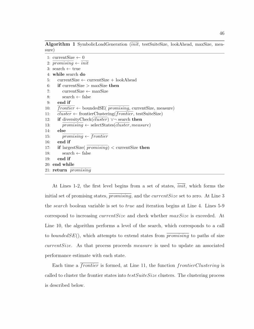
46

Algorithm 1 SymbolicLoadGeneration (init, testSuiteSize, lookAhead, maxSize, mea-sure)

1: currentSize ← 02: promising ← init3: search ← true4: while search do5: currentSize ← currentSize + lookAhead6: if currentSize > maxSize then7: currentSize ← maxSize8: search ← false9: end if

10: frontier ← boundedSE( promising, currentSize, measure)11: cluster ← frontierClustering(frontier, testSuiteSize)12: if diversityCheck(cluster) ∨¬ search then13: promising ← selectStates(cluster,measure)14: else15: promising ← frontier16: end if17: if largestSize( promising) < currentSize then18: search ← false19: end if20: end while21: return promising

At Lines 1-2, the first level begins from a set of states, init, which forms the

initial set of promising states, promising, and the currentSize set to zero. At Line 3

the search boolean variable is set to true and iteration begins at Line 4. Lines 5-9

correspond to increasing currentSize and check whether maxSize is exceeded. At

Line 10, the algorithm performs a level of the search, which corresponds to a call

to boundedSE(), which attempts to extend states from promising to paths of size

currentSize. As that process proceeds measure is used to update an associated

performance estimate with each state.

Each time a frontier is formed, at Line 11, the function frontierClustering is

called to cluster the frontier states into testSuiteSize clusters. The clustering process

is described below.

47

The goal of clustering is to identify sets of states that are behaviorally diverse—we

measure diversity by differences in the branch decisions required to reach a state. If

the clusters of states on the frontier are not sufficiently diverse, then we continue

with another level of symbolic execution that attempts to extend the entire frontier

another lookAhead branches. Should the current cluster pass the diversityCheck,

the function selectStates() selects the state from each cluster with the maximum

accumulated value for the performance measure (Line 13). Otherwise, the whole

frontier is copied over to the set of promising states and the search resumes (Line

15). We discuss several such measures in Section 3.4.

The iterative-deepening search terminates if no promising state has a path con-

dition whose size is lookAhead greater than the previous level’s states (Lines 17-18.

largestSize() returns the largest path condition found in promising).

When the search terminates, the path conditions associated with the promising

states can be solved with the support of a constraint solver to generate tests as is

done by existing automated generation approaches for functional tests.

3.3.1 Parameterizing SLG

In defining init a test engineer selects the portion of a program’s input that is treated

symbolically. Depending on the program one might, for example, fix the size or

structure of the input and let the values be symbolic. An example of the former case

is load testing of a program that processes inputs of uniform type but of varying size,

such as the JZlib compression program. An example of the latter case is load testing

of a program that processes structured input, such as the SQL query engine we study.

For such a program the structure may be fixed, e.g., the number of columns to select,

number of where clauses, etc., in the query, but the column names and where clause

expressions are symbolic. In general, treating more inputs symbolically will generate

48

more diverse and higher quality load test suites, but such a test generation may also

incur greater cost. We expect that in practice, test engineers will start with a small

set of symbolic inputs and then explore larger sized inputs to confirm the observations

made on smaller inputs.

The testSuiteSize parameter determines how many tests are to be generated.

Varying this parameter helps to produce a more comprehensive non-functional test

suite for the application under test. Regardless of the size of the test suite, SLG

always attempts to maximize diversity among tests. Exactly how many tests are

required to perform a thorough testing on the non-functional aspect of interest of the

application, however, is a harder question which cannot be assessed with traditional

test-adequacy measures, such as code coverage. In practice, selecting a test suite size

will likely be an iterative process where test suite size is increased until a point of

diminishing returns is reached [105]—where additional tests either lack diversity or a

high load.

Bounding the depth of symbolic execution is a common technique to control test

generation cost — the maxSize parameter achieves this in our approach. The param-

eter lookAhead, however, is particular to an iterative-deepening search as it regulates

how much distance the search advances in one iteration. The larger the lookAhead,

the more SLG resembles a full symbolic execution. Normally a smaller value for

lookAhead is desired, because a finer granularity would provide more opportunity for

state pruning, which is key to the efficiency of our approach. Ultimately state prun-

ing is decided by the diversity among the frontier of states, so a smaller lookAhead

alone cannot lead to ill-informed pruning. Setting lookAhead too small may cause

efficiency issues — a value of 1 will degrade the search to breadth first.

Figure 3.4 provides support for this intuition by plotting the quality of tests gen-

erated by our approach using lookAhead values of 1, 10, 50, 100, 500, 1000 and 30

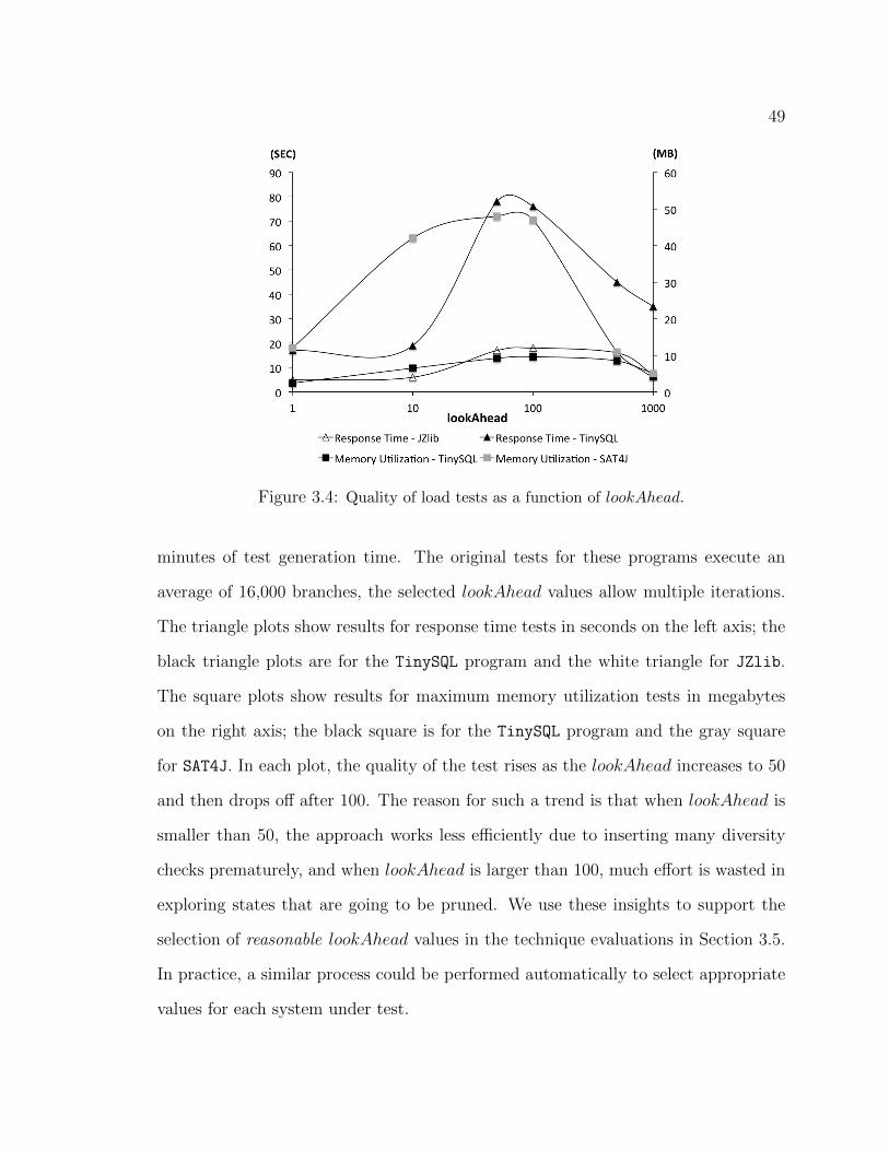
49

Figure 3.4: Quality of load tests as a function of lookAhead.

minutes of test generation time. The original tests for these programs execute an

average of 16,000 branches, the selected lookAhead values allow multiple iterations.

The triangle plots show results for response time tests in seconds on the left axis; the

black triangle plots are for the TinySQL program and the white triangle for JZlib.

The square plots show results for maximum memory utilization tests in megabytes

on the right axis; the black square is for the TinySQL program and the gray square

for SAT4J. In each plot, the quality of the test rises as the lookAhead increases to 50

and then drops off after 100. The reason for such a trend is that when lookAhead is

smaller than 50, the approach works less efficiently due to inserting many diversity

checks prematurely, and when lookAhead is larger than 100, much effort is wasted in

exploring states that are going to be pruned. We use these insights to support the

selection of reasonable lookAhead values in the technique evaluations in Section 3.5.

In practice, a similar process could be performed automatically to select appropriate

values for each system under test.

50

The last parameter, measure, defines how the approach should bias the search to

favor paths that are more costly in terms of the non-functional measure of interest.

The details of how the cost for a path is accumulated as the path is traversed and

associated with the end state of that path, which is implemented within boundedSE(),

and then used to select promising states, which is implemented in selectStates(), are

abstracted in Algorithm 1. In general, our approach can accommodate many measures

by simply associating different cost schemes with the code structures associated with

a path. In our studies we explore response time and maximum memory consumption

measures through the following cost computations:

a) Response Time Cost. This is a cumulative cost, so the maximal value occurs

at the end of the path. We estimate response time by accumulating the cost of each

bytecode. We use a very simple and configurable platform-independent cost model

that assigns different weights to bytecodes based on their associated cost.

b) Maximal Memory Usage Cost. It attempts to record the largest amount of

memory used at any point during a program execution by tracking operations that

allocate/deallocate memory and increment/decrement a memory usage value by a

quantity that reflects the object footprint of the allocated type. The maximal memory

value is only updated if the current usage value exceeds it. As with response time,

we find that this simple platform-independent approach strongly correlates to actual

memory consumption.

Independent of the chosen performance measure and cost, our approach assumes

that the measure constitutes part of a performance test oracle. We note that there is a

large number of measures explored in the literature, and that they are often specified

in the context of stochastic and queueing models [17], extended process algebras [62],

programmatic extensions [43], or concerted and early engineering efforts focused on

software performance [113]. Because such performance specifications are generally

51

still hard to find, we take a more pragmatic approach by leveraging the concept of a

differential test oracle. The idea behind differential oracles is to compare the system

performance across successive versions of an evolving system to detect performance

regressions, across competing systems performing the same functionality to detect

potential anomalies or disadvantageous settings, or across a series of inputs considered

equivalent to assess a systems’s sensitivity to variations in common situations.

3.3.2 Clustering the Frontier and Diversity Checks

A convenient choice of clustering would be to use the classic K-Means algorithm [61]

and define the number of unique clauses between two PCs as the clustering distance.

However, this would require comparing across all pairs of PCs of frontier states and

quickly run into scalability issues. For example, for the tinySQL program, clustering

a frontier into 10 clusters at depth 50 requires 2 seconds of execution time, but at

depth 100 would require 7 seconds. Doubling the depth caused 3.5 times increase in

processing time. In fact, the cost grows exponentially in terms of the explored depth.

To address this challenge, we devised an approximate algorithm that is linear in

the number of frontier states. It makes use of the intuition that for frontier states

resulting from a depth first search, a pair of neighboring states are more likely to

resemble each other than a pair of distant states. Algorithm 2 details the process. It

takes frontier and the size of resulting cluster K as input, where K is the number

of tests to be generated.

At Lines 3-5, it first computes the gap, in terms of the number of unique clauses,

between each pair of pc(si) and pc(si+1). At Line 6 it sorts the resulting gap vector

to find the largest K−1 gaps. At Lines 7-13, the algorithm uses the position of these

K − 1 largest gaps to partition the frontier into K clusters of various sizes.

The diversity check ensures that the gaps used to partition the frontier are of

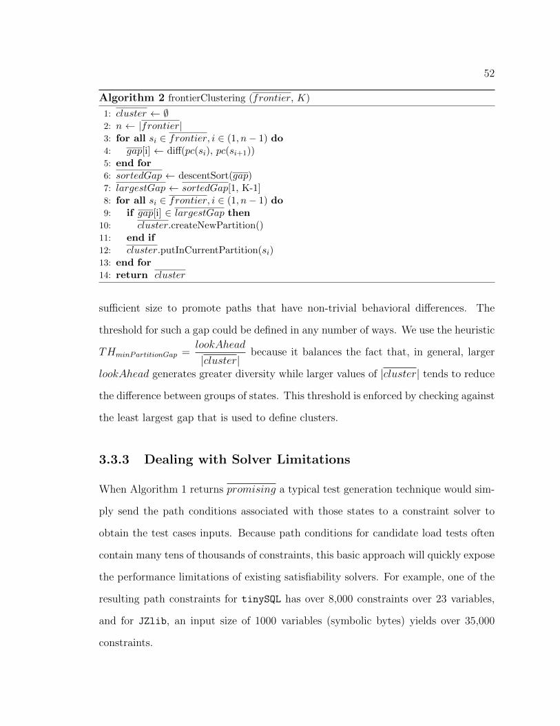
52

Algorithm 2 frontierClustering (frontier, K)

1: cluster ← ∅2: n ← |frontier|3: for all si ∈ frontier, i ∈ (1, n− 1) do4: gap[i] ← diff(pc(si), pc(si+1))5: end for6: sortedGap ← descentSort(gap)7: largestGap ← sortedGap[1, K-1]8: for all si ∈ frontier, i ∈ (1, n− 1) do9: if gap[i] ∈ largestGap then

10: cluster.createNewPartition()11: end if12: cluster.putInCurrentPartition(si)13: end for14: return cluster

sufficient size to promote paths that have non-trivial behavioral differences. The

threshold for such a gap could be defined in any number of ways. We use the heuristic

THminPartitionGap =lookAhead

|cluster|because it balances the fact that, in general, larger

lookAhead generates greater diversity while larger values of |cluster| tends to reduce

the difference between groups of states. This threshold is enforced by checking against

the least largest gap that is used to define clusters.

3.3.3 Dealing with Solver Limitations

When Algorithm 1 returns promising a typical test generation technique would sim-

ply send the path conditions associated with those states to a constraint solver to

obtain the test cases inputs. Because path conditions for candidate load tests often

contain many tens of thousands of constraints, this basic approach will quickly expose

the performance limitations of existing satisfiability solvers. For example, one of the

resulting path constraints for tinySQL has over 8,000 constraints over 23 variables,

and for JZlib, an input size of 1000 variables (symbolic bytes) yields over 35,000

constraints.

53

Algorithm 3 ConstraintLimitedLoadGeneration(init, testSuiteSize, lookAhead, maxSize,measure, maxSolverConstraints)

1: currentSize ← maxSolverConstraints2: while currentSize < maxSize do3: promising ← SymbolicLoadGen(init, testSuiteSize, lookAhead, maxSolverCon-

straints, measure)4: init← ∅5: for s ∈ promising do6: inputs← solve(pc(s))7: init← init ∪ stateAfterReplay(inputs, pc(s))8: end for9: currentSize ← currentSize + maxSolverConstraints

10: end while11: return promising

We address this issue by defining an outer search, Algorithm 3, that wraps calls

to Algorithm 1 in such a way that the maximum number of symbolic constraints

considered within any one invocation of Algorithm 1 is bounded. ConstraintLimit-

edLoadGeneration(CLLG) takes the same parameters as SLG plus an additional

parameter maxSolverConstraints. This parameter can be configured based on the

scalability of the constraint solver used to implement symbolic execution.

Algorithm 1 is invoked with maxSolverConstraints as the maxSize parameter

that governs the overall size of the iterative-deepening symbolic execution. At Line 3,

the iteration starts by invoking SLG to compute the current set of promising states.

When promising is returned, Algorithm 3 solves the path constraints of each state

in promising to obtain the input values necessary to reach those states (Line 6).

Then, it replays the program using those concrete inputs and, when the program

has traversed all the predicates in the path condition, the program state is captured

and added to init (Line 7). The algorithm terminates when the sum of sizes of the

path conditions explored in each of the invocations of SymbolicLoadGen() exceeds

the maxSize.

In essence, Algorithm 3 increases the scalability of our approach by chaining par-

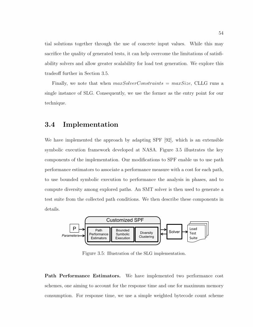
54

tial solutions together through the use of concrete input values. While this may

sacrifice the quality of generated tests, it can help overcome the limitations of satisfi-

ability solvers and allow greater scalability for load test generation. We explore this

tradeoff further in Section 3.5.

Finally, we note that when maxSolverConstraints = maxSize, CLLG runs a

single instance of SLG. Consequently, we use the former as the entry point for our

technique.

3.4 Implementation

We have implemented the approach by adapting SPF [92], which is an extensible

symbolic execution framework developed at NASA. Figure 3.5 illustrates the key

components of the implementation. Our modifications to SPF enable us to use path

performance estimators to associate a performance measure with a cost for each path,

to use bounded symbolic execution to performance the analysis in phases, and to

compute diversity among explored paths. An SMT solver is then used to generate a

test suite from the collected path conditions. We then describe these components in

details.

Load Test Suite

Solver Path Performance Estimators

Bounded Symbolic Execution

Diversity Clustering

Customized SPF

P Parameters

Figure 3.5: Illustration of the SLG implementation.

Path Performance Estimators. We have implemented two performance cost

schemes, one aiming to account for the response time and one for maximum memory

consumption. For response time, we use a simple weighted bytecode count scheme

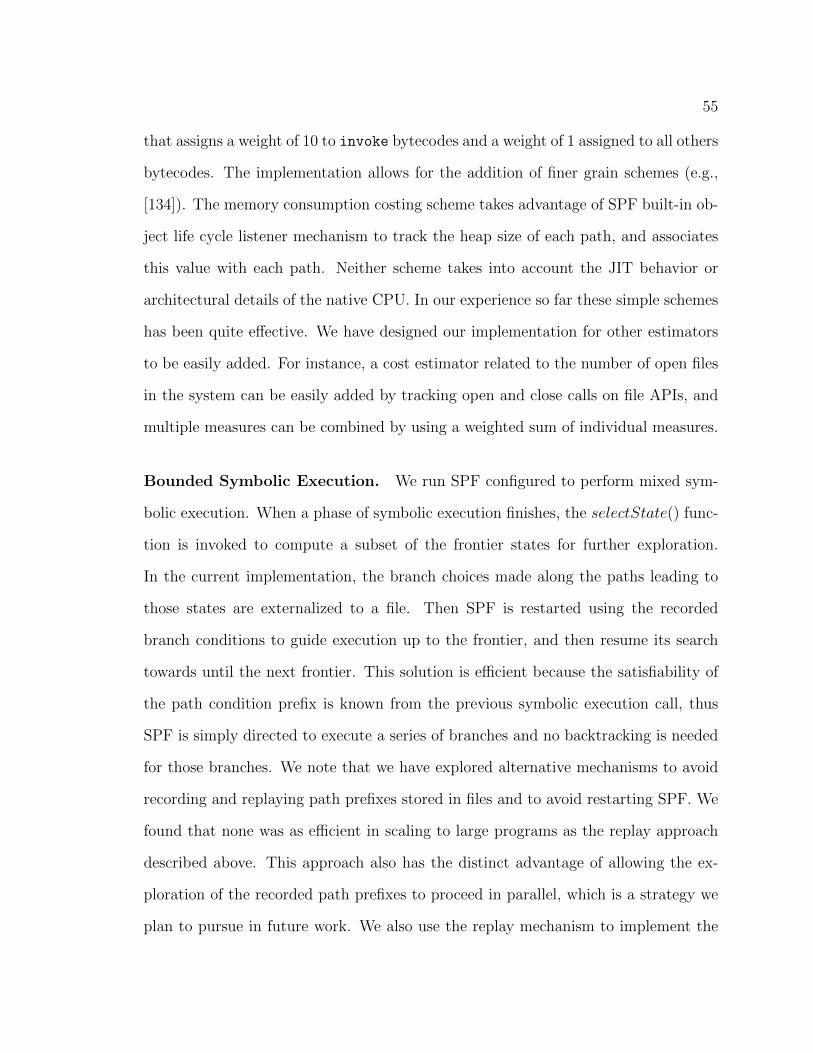
55

that assigns a weight of 10 to invoke bytecodes and a weight of 1 assigned to all others

bytecodes. The implementation allows for the addition of finer grain schemes (e.g.,

[134]). The memory consumption costing scheme takes advantage of SPF built-in ob-

ject life cycle listener mechanism to track the heap size of each path, and associates

this value with each path. Neither scheme takes into account the JIT behavior or

architectural details of the native CPU. In our experience so far these simple schemes

has been quite effective. We have designed our implementation for other estimators

to be easily added. For instance, a cost estimator related to the number of open files

in the system can be easily added by tracking open and close calls on file APIs, and

multiple measures can be combined by using a weighted sum of individual measures.

Bounded Symbolic Execution. We run SPF configured to perform mixed sym-

bolic execution. When a phase of symbolic execution finishes, the selectState() func-

tion is invoked to compute a subset of the frontier states for further exploration.

In the current implementation, the branch choices made along the paths leading to

those states are externalized to a file. Then SPF is restarted using the recorded

branch conditions to guide execution up to the frontier, and then resume its search

towards until the next frontier. This solution is efficient because the satisfiability of

the path condition prefix is known from the previous symbolic execution call, thus

SPF is simply directed to execute a series of branches and no backtracking is needed

for those branches. We note that we have explored alternative mechanisms to avoid

recording and replaying path prefixes stored in files and to avoid restarting SPF. We

found that none was as efficient in scaling to large programs as the replay approach

described above. This approach also has the distinct advantage of allowing the ex-

ploration of the recorded path prefixes to proceed in parallel, which is a strategy we

plan to pursue in future work. We also use the replay mechanism to implement the

56

stateAfterReplay() function used in Algorithm 3.3.3.

Diversity Clustering. Algorithm 2 takes advantage of the SPF backtracking sup-

port to efficiently compute the gap vector on the fly, because each gap between two

states si and si+1 equals the number of branches si needs to backtrack before it can

continue on a new path that leads to si+1.

Test Instantiation. Generating tests from a path condition requires the ability to

both solve and produce a model for a given formula. We have explored the use of

several constraint and SMT solvers, including Choco [26] (Version 2.04), CVC3 [30]

(Version 3.2), and Yices [131] (Version 1.0.12) in a period between Fall 2009 and

Summer 2010. Our integration of Yices into SPF has greatly improved the scalability

of SPF in general and of our technique in particular. The data reported in our study

uses this Yices-based implementation.

3.5 Evaluation

Our assessment takes on multiple dimensions, resources, and artifacts.

First, we assess the approach configured to induce large response times and com-

pared it against random test generation. Then, we explore the scalability of various

instantiations of the approach. We do this in the context of JZlib [69] (5633 LOC4), a

Java re-implementation of the popular Zlib package. This program is well suited for

the study because we can easily and incrementally increase the input size (from 1KB

to 100MB) to investigate the scalability of the approach and response time is one of

its two key performance evaluation criteria. Moreover, we can easily generate what

the Spec2000 benchmark documentation [114] defines as the worst load test inputs for

4LOC stands for ‘Lines Of Code’ of a program.

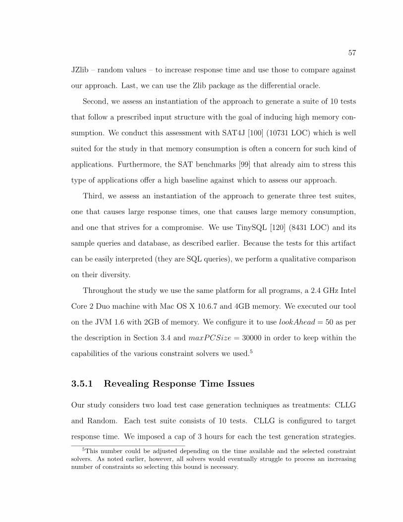
57

JZlib – random values – to increase response time and use those to compare against

our approach. Last, we can use the Zlib package as the differential oracle.

Second, we assess an instantiation of the approach to generate a suite of 10 tests

that follow a prescribed input structure with the goal of inducing high memory con-

sumption. We conduct this assessment with SAT4J [100] (10731 LOC) which is well

suited for the study in that memory consumption is often a concern for such kind of

applications. Furthermore, the SAT benchmarks [99] that already aim to stress this

type of applications offer a high baseline against which to assess our approach.

Third, we assess an instantiation of the approach to generate three test suites,

one that causes large response times, one that causes large memory consumption,

and one that strives for a compromise. We use TinySQL [120] (8431 LOC) and its

sample queries and database, as described earlier. Because the tests for this artifact

can be easily interpreted (they are SQL queries), we perform a qualitative comparison

on their diversity.

Throughout the study we use the same platform for all programs, a 2.4 GHz Intel

Core 2 Duo machine with Mac OS X 10.6.7 and 4GB memory. We executed our tool

on the JVM 1.6 with 2GB of memory. We configure it to use lookAhead = 50 as per

the description in Section 3.4 and maxPCSize = 30000 in order to keep within the

capabilities of the various constraint solvers we used.5

3.5.1 Revealing Response Time Issues

Our study considers two load test case generation techniques as treatments: CLLG

and Random. Each test suite consists of 10 tests. CLLG is configured to target

response time. We imposed a cap of 3 hours for each the test generation strategies.

5This number could be adjusted depending on the time available and the selected constraintsolvers. As noted earlier, however, all solvers would eventually struggle to process an increasingnumber of constraints so selecting this bound is necessary.

58

Figure 3.6: Revealing performance issues: response time differences of JZlib vs Zlib whenusing testing suites generated by CLLG vs Random.

Strategies requiring more time were terminated and not reported as part of the series.

For Random test generation we used the whole allocation of 3 hours to simplify the

study design, which is conservative in that it may overestimate the effectiveness of

the Random test suites in cases were the CLLG suites for the same input size took

less than 3 hours to generate. For the Random treatment, we use a random byte

generator to create the file streams to be expanded. Another consideration with

Random is that, unlike our approach with its built-in selection mechanism, it does

not include a process to distinguish the best 10 load tests. This is important as

Random can quickly generate millions of tests from which only a small percentage

may be worth retaining as part of a load test suite. To enable the identification of such

tests, we simply run each test generated by Random once and record its execution

time. This execution time, although generally brief, is included in the overall test

case generation time.

We first compare the response times of JZlib caused by tests generated with

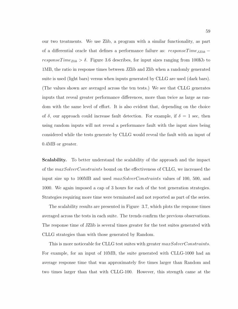
59

our two treatments. We use Zlib, a program with a similar functionality, as part

of a differential oracle that defines a performance failure as: responseT imeJZlib −

responseT imeZlib > δ. Figure 3.6 describes, for input sizes ranging from 100Kb to

1MB, the ratio in response times between JZlib and Zlib when a randomly generated

suite is used (light bars) versus when inputs generated by CLLG are used (dark bars).

(The values shown are averaged across the ten tests.) We see that CLLG generates

inputs that reveal greater performance differences, more than twice as large as ran-

dom with the same level of effort. It is also evident that, depending on the choice

of δ, our approach could increase fault detection. For example, if δ = 1 sec, then

using random inputs will not reveal a performance fault with the input sizes being

considered while the tests generate by CLLG would reveal the fault with an input of

0.4MB or greater.

Scalability. To better understand the scalability of the approach and the impact

of the maxSolverConstraints bound on the effectiveness of CLLG, we increased the

input size up to 100MB and used maxSolverConstraints values of 100, 500, and

1000. We again imposed a cap of 3 hours for each of the test generation strategies.

Strategies requiring more time were terminated and not reported as part of the series.

The scalability results are presented in Figure 3.7, which plots the response times

averaged across the tests in each suite. The trends confirm the previous observations.

The response time of JZlib is several times greater for the test suites generated with

CLLG strategies than with those generated by Random.

This is more noticeable for CLLG test suites with greater maxSolverConstraints.

For example, for an input of 10MB, the suite generated with CLLG-1000 had an

average response time that was approximately five times larger than Random and

two times larger than that with CLLG-100. However, this strength came at the

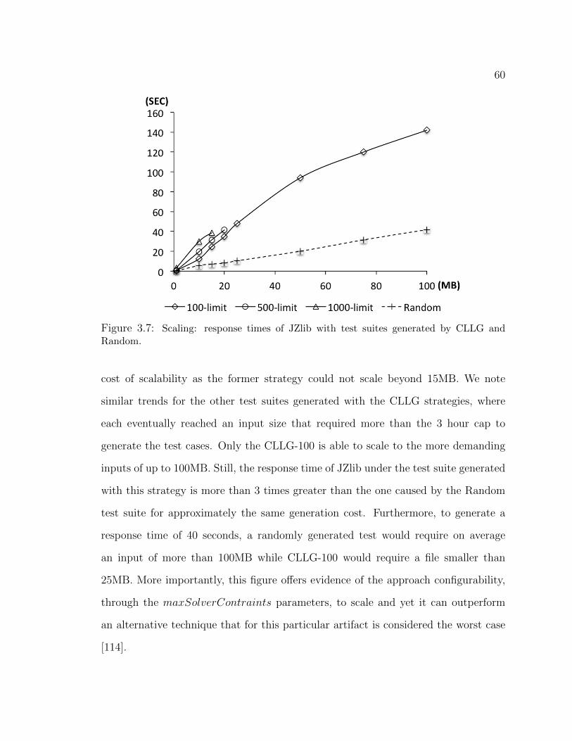
60

Figure 3.7: Scaling: response times of JZlib with test suites generated by CLLG andRandom.

cost of scalability as the former strategy could not scale beyond 15MB. We note

similar trends for the other test suites generated with the CLLG strategies, where

each eventually reached an input size that required more than the 3 hour cap to

generate the test cases. Only the CLLG-100 is able to scale to the more demanding

inputs of up to 100MB. Still, the response time of JZlib under the test suite generated

with this strategy is more than 3 times greater than the one caused by the Random

test suite for approximately the same generation cost. Furthermore, to generate a

response time of 40 seconds, a randomly generated test would require on average

an input of more than 100MB while CLLG-100 would require a file smaller than

25MB. More importantly, this figure offers evidence of the approach configurability,

through the maxSolverContraints parameters, to scale and yet it can outperform

an alternative technique that for this particular artifact is considered the worst case

[114].

61

3.5.2 Revealing Memory Consumption Issues

We now proceed to assess 5 test suites of 10 tests generated by our approach to induce

high memory consumption in SAT4J. We randomly chose 5 benchmarks from the SAT

competition 2009 suite to get a pool of potential values for the number of variables,

number of clauses and the number of variables within each clause, and we declare

the variables themselves as symbolic. Columns 2 to 4 of Table 3.1 show some of the

attributes of the selected benchmarks including the number of variables, number of

clauses, and hardness level (assigned based on the results of past competitions, with

instances solved within 30 seconds by all solvers labelled as “easy,” not solved by any

solver within the timeout of the event labelled as “hard,” and “medium” for the rest.)

Table 3.1 shows the memory consumption results in the last two columns. Column

“Original” shows memory consumption of SAT4J when these benchmark programs

are provided as inputs, column “Generated” shows the same measure for the average

of the ten tests generated with our approach, and Column “% Increase” shows the

increase generated tests have over original ones. Overall, the approach was effective

in increasing the memory load for SAT4J compared with the original benchmarks.

However, the gains are not uniform across instances. The most dramatic gain achieved

by our approach, 2.6 times increase in memory consumption, comes from selecting

values for aloul which is of “medium” hardness. Not surprisingly, the least significant

gain comes from rbcl-xits-06-UNSAT, which is classified as “hard.” But even for

this input with a very large and challenging space of over 47000 clauses the approach

leads to the generation of a test suite that on average consumes 20% more memory.

62

Table 3.1: Load test generation for memory consumption.

ProgramsDescription Memory (MB)

Variables Clauses HardnessOriginal Generated % Increasealoul-chnl11-13 286 1742 medium 6 22 260%cmu-bmc-longmult15 7807 24351 easy 35 92 163%eq-atree-braun-8-unsat 684 2300 medium 11 35 218%rbcl-xits-06-UNSAT 980 47620 hard 38 45 19%unif-k3-r4.25 480 2040 medium 6 17 183%

Table 3.2: Response time and memory consumption for test suites designed to increasethose performance measures in isolation (TS-RT and TS-MEM) and jointly (TS-RT-MEM).

Test Suite Response Time Memory ConsumptionSeconds % over Baseline MB % over Baseline

Baseline 45 100 6.6 100TS-RT 105 234 13 196TS-MEM 98 217 15 219TS-RT-MEM 96 213 13 201

3.5.3 Load inducing tests across resources and test diversity

We now assess the approach in the presence of different performances measures and

in terms of the diversity of the test suite it generates.

We generate three test suites with 5 tests each for TinySQL (in this study we

generate 5 tests instead of 10 because we intentionally want to increase the level of

diversity among tests). The first, TS-RT, favors response time. The second, TS-

MEM, favors memory consumption. The third, TS-RT-MEM, was generated with

an equally weighted sum of the cost for response time and memory consumption.

Table 3.2 shows the performance caused by each test suite averaged across the five

tests. We use as baseline the original test from which the test template was derived.

We report both response time and memory consumption, along with their respective

effectiveness over the baseline, for each suite.

The results show that all three test suites are effective at increasing their respective

measures. On average, TS-RT forces response times to rise 234% over the baseline,

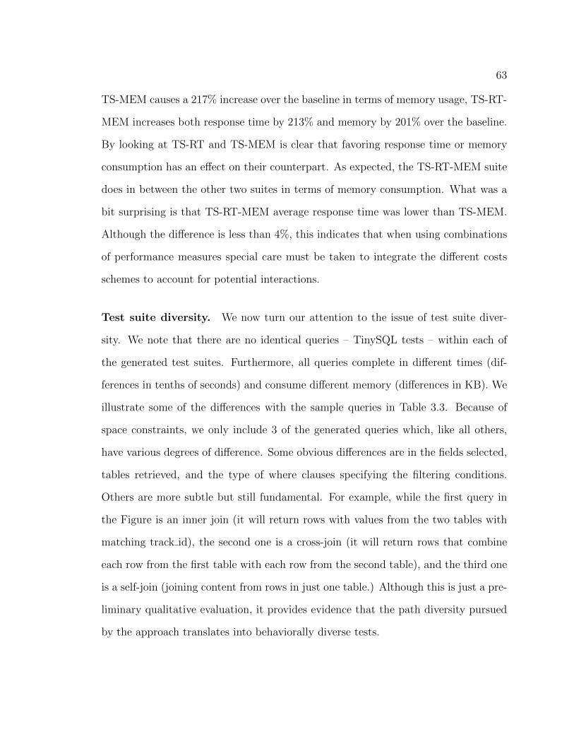
63

TS-MEM causes a 217% increase over the baseline in terms of memory usage, TS-RT-

MEM increases both response time by 213% and memory by 201% over the baseline.

By looking at TS-RT and TS-MEM is clear that favoring response time or memory

consumption has an effect on their counterpart. As expected, the TS-RT-MEM suite

does in between the other two suites in terms of memory consumption. What was a

bit surprising is that TS-RT-MEM average response time was lower than TS-MEM.

Although the difference is less than 4%, this indicates that when using combinations

of performance measures special care must be taken to integrate the different costs

schemes to account for potential interactions.

Test suite diversity. We now turn our attention to the issue of test suite diver-

sity. We note that there are no identical queries – TinySQL tests – within each of

the generated test suites. Furthermore, all queries complete in different times (dif-

ferences in tenths of seconds) and consume different memory (differences in KB). We

illustrate some of the differences with the sample queries in Table 3.3. Because of

space constraints, we only include 3 of the generated queries which, like all others,

have various degrees of difference. Some obvious differences are in the fields selected,

tables retrieved, and the type of where clauses specifying the filtering conditions.

Others are more subtle but still fundamental. For example, while the first query in

the Figure is an inner join (it will return rows with values from the two tables with

matching track id), the second one is a cross-join (it will return rows that combine

each row from the first table with each row from the second table), and the third one

is a self-join (joining content from rows in just one table.) Although this is just a pre-

liminary qualitative evaluation, it provides evidence that the path diversity pursued

by the approach translates into behaviorally diverse tests.

64

Table 3.3: Queries illustrating test suite diversity.

SELECT MUSIC TRACKS.track name, MUSIC TRACKS.track idFROM MUSIC TRACKSJOIN MUSIC COLLECTION ON

MUSIC TRACKS.track id = MUSIC COLLECTION.track idWHERE MUSIC TRACKS.track name <> null OR

MUSIC TRACKS.track id > 0SELECT MUSIC ARTISTS.artst id, MUSIC ARTISTS.artst nameFROM MUSIC ARTISTSJOIN MUSIC EVENTS ON

MUSIC ARTISTS.artstid <> nullWHERE MUSIC ARTISTS.artst name <> null OR

MUSIC ARTISTS.artst id > 0SELECT MUSIC ARTISTS.artst name, MUSIC ARTISTS.artst countryFROM MUSIC ARTISTSJOIN MUSIC ARTISTS ON

MUSIC ARTISTS.artst name <> MUSIC ARTISTS.artst nameWHERE MUSIC ARTISTS.artst id > 5 OR

MUSIC ARTISTS.artst country <> null

3.6 Summary

So far we have introduced SLG, a symbolic execution based technique capable of

generating load test suite automatically. Our assessment of SLG shows that it can

induce program loads across different types of resources that are significantly better

than alternative approaches (randomly generated tests in the first study, a standard

benchmark in the second study, and the default suite in the third study). However,

as we will show later in Section 4.1, the cost of generating tests still grows between

linearly or exponentially with SLG as program or input size increases. In the next

chapter we present a new approach that aims at scaling up the load test generation

technique, which uses SLG as a subroutine in its own analysis.

65

Chapter 4

Compositional Load Test

Generation

In this chapter we present our effort in scaling up the load test generation tech-

nique. In Section 4.1, we discuss the problems that our load test generation tool SLG

faces when applied to more complex software systems. In Section 4.2 - Section 4.4

we present a compositional load test generation technique, CompSLG, that enables

handling of complex systems in the form of software pipelines; the algorithms and pa-

rameters that controls the techniques; and its implementation details. In Section 4.5

we evaluate CompSLG on four Unix pipeline programs and one XML pipeline. The re-

sults show that when reuse of previous analysis results is allowed, CompSLG achieves

orders of magnitude savings in test generation time, while maintaining the same level

of induced load as SLG. Finally, in Section 4.6, we discuss the challenges on extending

CompSLG to enabled handling of more complex systems beyond software pipelines.

We present an approach and implementation sketch for handling Java programs, and

provide several proof-of-concept examples to show its viability.1

1Portions of the material presented in this chapter have appeared previously in a paper byZhang et al. [138]. The material presented in this chapter extends the technique to enable load test

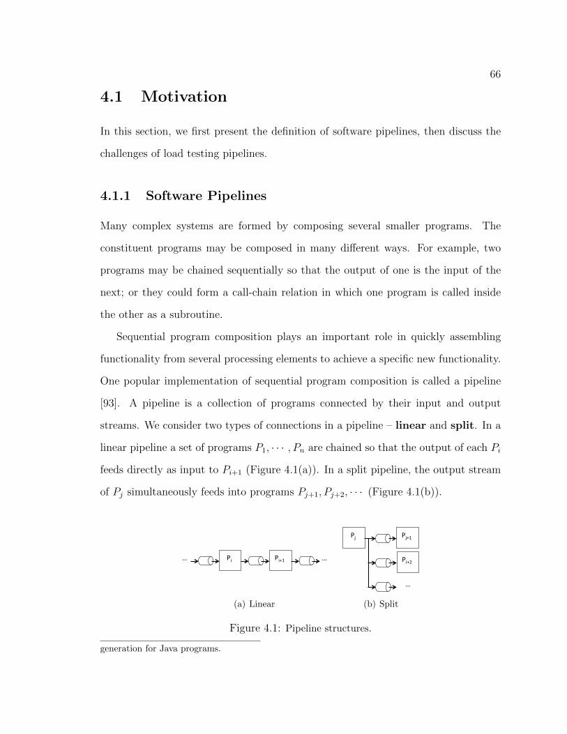
66

4.1 Motivation

In this section, we first present the definition of software pipelines, then discuss the

challenges of load testing pipelines.

4.1.1 Software Pipelines

Many complex systems are formed by composing several smaller programs. The

constituent programs may be composed in many different ways. For example, two

programs may be chained sequentially so that the output of one is the input of the

next; or they could form a call-chain relation in which one program is called inside

the other as a subroutine.

Sequential program composition plays an important role in quickly assembling

functionality from several processing elements to achieve a specific new functionality.

One popular implementation of sequential program composition is called a pipeline

[93]. A pipeline is a collection of programs connected by their input and output

streams. We consider two types of connections in a pipeline – linear and split. In a

linear pipeline a set of programs P1, · · · , Pn are chained so that the output of each Pi

feeds directly as input to Pi+1 (Figure 4.1(a)). In a split pipeline, the output stream

of Pj simultaneously feeds into programs Pj+1, Pj+2, · · · (Figure 4.1(b)).

…"Pi"…" Pi+1"

Pj" Pj+1"

Pi+2"

…"

(a) Linear

…"Pi"…" Pi+1"

Pj" Pj+1"

Pi+2"

…"

(b) Split

Figure 4.1: Pipeline structures.

generation for Java programs.

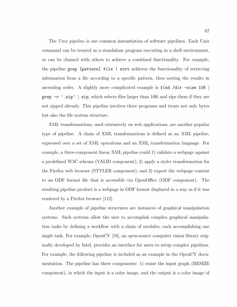
67

The Unix pipeline is one common instantiation of software pipelines. Each Unix

command can be treated as a standalone program executing in a shell environment,

or can be chained with others to achieve a combined functionality. For example,

the pipeline grep [pattern] file | sort achieves the functionality of retrieving

information from a file according to a specific pattern, then sorting the results in

ascending order. A slightly more complicated example is find /dir -size 10K |

grep -v ’.zip’ | zip, which selects files larger than 10K and zips them if they are

not zipped already. This pipeline involves three programs and treats not only bytes

but also the file system structure.

XML transformations, used extensively on web applications, are another popular

type of pipeline. A chain of XML transformations is defined as an XML pipeline,

expressed over a set of XML operations and an XML transformation language. For

example, a three-component linear XML pipeline could 1) validate a webpage against

a predefined W3C schema (VALID component); 2) apply a styler transformation for

the Firefox web browser (STYLER component); and 3) export the webpage content

to an ODF format file that is accessible via OpenOffice (ODF component). The

resulting pipeline product is a webpage in ODF format displayed in a way as if it was

rendered by a Firefox browser [112].

Another example of pipeline structures are instances of graphical manipulation

systems. Such systems allow the user to accomplish complex graphical manipula-

tion tasks by defining a workflow with a chain of modules, each accomplishing one

single task. For example, OpenCV [19], an open-source computer vision library orig-

inally developed by Intel, provides an interface for users to setup complex pipelines.

For example, the following pipeline is included as an example in the OpenCV docu-

mentation. The pipeline has three components: 1) resize the input graph (RESIZE

component), in which the input is a color image, and the output is a color image of

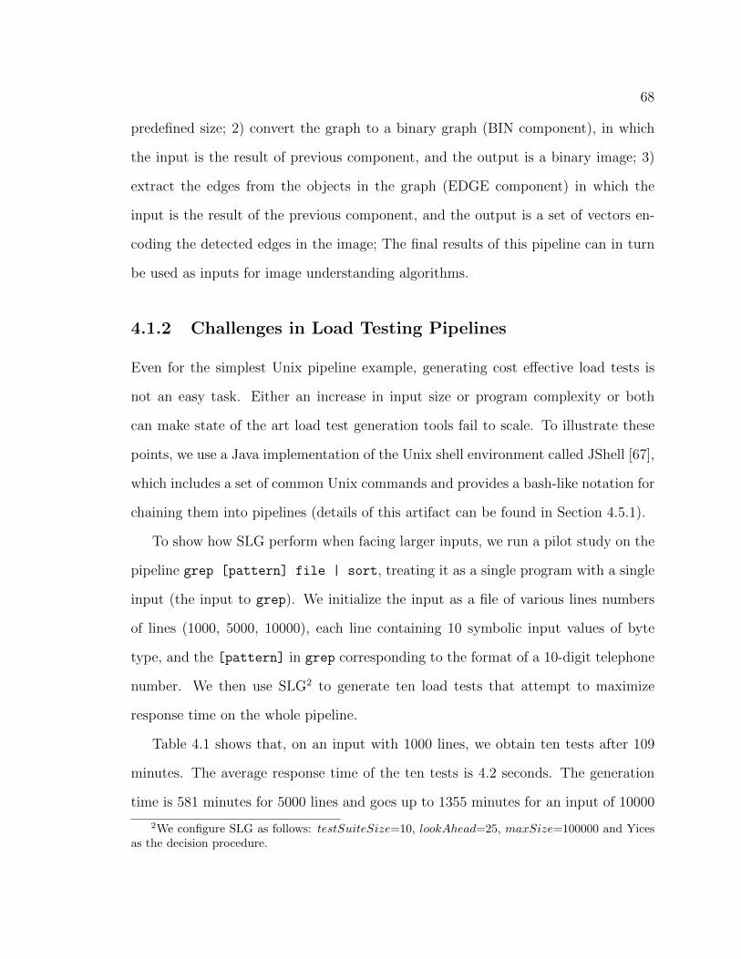
68

predefined size; 2) convert the graph to a binary graph (BIN component), in which

the input is the result of previous component, and the output is a binary image; 3)

extract the edges from the objects in the graph (EDGE component) in which the

input is the result of the previous component, and the output is a set of vectors en-

coding the detected edges in the image; The final results of this pipeline can in turn

be used as inputs for image understanding algorithms.

4.1.2 Challenges in Load Testing Pipelines

Even for the simplest Unix pipeline example, generating cost effective load tests is

not an easy task. Either an increase in input size or program complexity or both

can make state of the art load test generation tools fail to scale. To illustrate these

points, we use a Java implementation of the Unix shell environment called JShell [67],

which includes a set of common Unix commands and provides a bash-like notation for

chaining them into pipelines (details of this artifact can be found in Section 4.5.1).

To show how SLG perform when facing larger inputs, we run a pilot study on the

pipeline grep [pattern] file | sort, treating it as a single program with a single

input (the input to grep). We initialize the input as a file of various lines numbers

of lines (1000, 5000, 10000), each line containing 10 symbolic input values of byte

type, and the [pattern] in grep corresponding to the format of a 10-digit telephone

number. We then use SLG2 to generate ten load tests that attempt to maximize

response time on the whole pipeline.

Table 4.1 shows that, on an input with 1000 lines, we obtain ten tests after 109

minutes. The average response time of the ten tests is 4.2 seconds. The generation

time is 581 minutes for 5000 lines and goes up to 1355 minutes for an input of 10000

2We configure SLG as follows: testSuiteSize=10, lookAhead=25, maxSize=100000 and Yicesas the decision procedure.

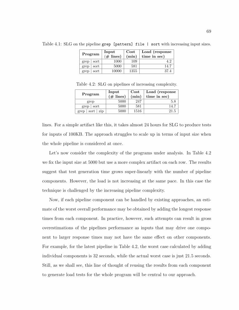
69

Table 4.1: SLG on the pipeline grep [pattern] file | sort with increasing input sizes.

ProgramInput Cost Load (response(# lines) (min) time in sec)

grep | sort 1000 109 4.2grep | sort 5000 581 14.7grep | sort 10000 1355 37.4

Table 4.2: SLG on pipelines of increasing complexity.


grep 5000 247 5.8grep | sort 5000 581 14.7

grep | sort | zip 5000 1516 21.5

lines. For a simple artifact like this, it takes almost 24 hours for SLG to produce tests

for inputs of 100KB. The approach struggles to scale up in terms of input size when

the whole pipeline is considered at once.

Let’s now consider the complexity of the programs under analysis. In Table 4.2

we fix the input size at 5000 but use a more complex artifact on each row. The results

suggest that test generation time grows super-linearly with the number of pipeline

components. However, the load is not increasing at the same pace. In this case the

technique is challenged by the increasing pipeline complexity.

Now, if each pipeline component can be handled by existing approaches, an esti-

mate of the worst overall performance may be obtained by adding the longest response

times from each component. In practice, however, such attempts can result in gross

overestimations of the pipelines performance as inputs that may drive one compo-

nent to larger response times may not have the same effect on other components.

For example, for the latest pipeline in Table 4.2, the worst case calculated by adding

individual components is 32 seconds, while the actual worst case is just 21.5 seconds.

Still, as we shall see, this line of thought of reusing the results from each component

to generate load tests for the whole program will be central to our approach.

70

4.2 Overview of a Compositional Approach

Although a large complex program imposes many challenges for a symbolic load test

generation approach, if the complex program is composed of several simpler programs,

such as the pipeline examples shown in the last section, and each constituent program

can be handled by existing approaches, we may devise a new approach that uses the

divide and conquer strategy to address the illustrated challenges.

Load#Test#Suite#

SLG##

Performance#Summaries#

P1# P2# …#

PS1#

PS2#

PSi#

Generate#Channeling#Constraints#

Find#Compa<ble#Summaries#

Constraints#Weighing#&#Relaxa<on#

Solver#

SLG##

SLG##

Sa,sfiability'test'a9er'each'relaxa,on''

Figure 4.2: Illustration of a compositional approach.

Figure 4.2 shows the key concepts of a compositional load test generation ap-

proach. The approach works in four steps. 1) The set of programs (e.g., P1, P2, · · · )

that form a software pipeline are analyzed by SLG to produce a library consisting

of performance summaries for each program. A performance summary characterizes

one program with a set of path constraints, each representing a program path that

induces load according to a performance measure. 2) The approach examines how the

constituent programs are composed together, and uses this information as a guide-

line for selecting compatible path constraints from the library. It also generates a

set of channeling constraints for each pair of programs. Channeling constraints are

equality constraints that bridge the variable sets of two performance summaries com-

puted independently. 3) The selected path constraints and the generated channeling

constraints are joined together by conjunction to form a constraint set for the whole

71

program. The resulting constraint set may not be solvable because each constituent

constraint encodes a load test of one component, which may not be compatible with

the load tests of the other components. Therefore, a constraint weighing and relax-

ation process is used to remove incompatible constraints, starting from the weakest

in terms of their contributions to the program load. The weighing and relaxation

process tests the satisfiability of the remaining constraint set after each removal. It

iterates until the end product becomes solvable. 4) A solver is used to find a solution

that satisfies the constraint set, leading to a load test for the whole program. Steps

2-4 are repeated until a load test suite of desired size is generated.

The approach in practice. Continuing with the grep [pattern] file | sort

example, we use the same settings as before, only this time we collect performance

summaries with SLG, then apply the compositional generation approach on them.

Figure 4.3 illustrates the approach3. For steps 1-2, we generate the performance

summaries for both grep and sort, choose one path constraint from each summary

(starting from the worst performing ones) and make sure they are compatible by

checking for matching output and input sizes (so that they can be executed in a

pipeline). The two selected path constraints are shown in Figure 4.3 on the leftmost

and rightmost columns. The center column shows the channeling constraints that

bridge the two path constraints (which are computed by tracking the output expres-

sions of grep in terms of its input variables). Section 4.3.2 describes in detail how to

compute the channeling constraints.

The third step involves the conjunction of the three constraint sets, and applying

a weighing and relaxation process to remove incompatible constraints. The process

starts by removing those constraints that make the least contribution to the load, so

3To simplify the presentation, Figure 4.3 depicts a case with the input size of 10 lines, where inthe pilot studies the input size varies between 1000 to 10,000 lines.

72

(g4$–$(9$–$g1))$<=$(g8$–$g1)$�$…$

g9$>$0$�$…$

((g8$–$g1)$+$(g3$–$(9$–$g1)))$<=$(g8$–$g1)$�$…$

(g4$–$(9$–$g1))$!=$0$�$(g3$–$(9$–$g1))$!=$0$�$(g2$–$(9$–$g1))$!=$0$�$

Path$Constraints$for$grep% Path$Constraints$for$sort%

s1$<$s2$�$s1$<$s3$�$s2$<$s6$�$

…$s4$<$s5$�$s4$<$s7$�$

…$s5$<$s6$�$

…$s5$<$s8$�$

Channeling$Constraints%s1$=$g1$�$s2$=$g4$�$s3$=$g5$�$s4$=$g6$�$s5$=$g7$�$s6$=$g8$�$s7$=$g9$�$s8$=$g3$

Figure 4.3: Path constraints computed for grep [pattern] file | sort, with the pat-tern being a 10-digit phone number. Three sets of constraints are shown, one for grep, onefor sort, one for the channeling constraints connecting them. Crossed out constraints havebeen removed in order to find a solution.

that the loss in load is minimized, and testing the satisfiability of the remaining ones

after each removal. Figure 4.3 depicts a situation where the incompatible constraints

have been removed (crossed out), and the remaining constraint set is satisfiable.

Table 4.3 shows the results of redoing the first pilot study (Table 4.1) with the

compositional approach. On 1000 lines of input, the approach generated tests of

similar quality (4.2 sec vs 4.1 sec) while the generation time is 32% lower. The

savings are more impressive as the input size goes up. On an input of 10000 lines,

the previous run used almost 24 hours, while the compositional approach finishes in

11 hours and generates tests that induce similar load.

Redoing the second pilot study yields more impressive results. Because the pro-

grams under study use the same input size on the three pipelines, the approach is

able to reuse the performance summaries collected from a previous artifact to achieve

more savings. For example, on analyzing grep | sort, we can reuse the summaries

computed for grep and only need to compute summaries for sort. Table 4.4 shows

that, in case of grep | sort | zip, the compositional approach takes only 12% of

the effort of a full SLG, but yields comparable tests.

In practice, the gains in efficiency can in turn improve effectiveness if the testing

effort is bounded. For example, assume that a tester is given three hours of test

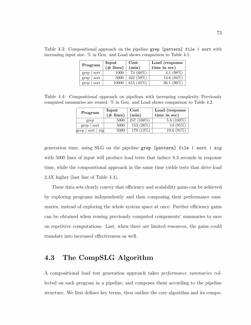
73

Table 4.3: Compositional approach on the pipeline grep [pattern] file | sort withincreasing input size. % in Gen. and Load shows comparison to Table 4.1.


grep | sort 1000 74 (68%) 4.1 (98%)grep | sort 5000 342 (59%) 13.6 (94%)grep | sort 10000 615 (45%) 36.1 (96%)

Table 4.4: Compositional approach on pipelines with increasing complexity Previouslycomputed summaries are reused. % in Gen. and Load shows comparison to Table 4.2.


grep 5000 247 (100%) 5.8 (100%)grep | sort 5000 153 (26%) 14 (95%)

grep | sort | zip 5000 179 (12%) 19.6 (91%)

generation time, using SLG on the pipeline grep [pattern] file | sort | zip

with 5000 lines of input will produce load tests that induce 8.3 seconds in response

time, while the compositional approach in the same time yields tests that drive load

2.4X higher (last line of Table 4.4).

These data sets clearly convey that efficiency and scalability gains can be achieved

by exploring programs independently and then composing their performance sum-

maries, instead of exploring the whole system space at once. Further efficiency gains

can be obtained when reusing previously computed components’ summaries to save

on repetitive computations. Last, when there are limited resources, the gains could

translate into increased effectiveness as well.

4.3 The CompSLG Algorithm

A compositional load test generation approach takes performance summaries col-

lected on each program in a pipeline, and composes them according to the pipeline

structure. We first defines key terms, then outline the core algorithm and its compo-

74

nents.

Definition 4.3.1 Performance Summary (PS): A set of path conditions PSsj =

{pcj1, · · · , pcjn} for program Pj caused by inputs of size s that induce load according to

a performance measure. Each pcji contains the following tags to assist future analysis:

size and type of the path’s input and output, and the weight score indicating the

level of resource consumption (load) when the path is executed.

A PSsj can be computed by applying any symbolic execution based load testing

approach (such as SLG) to program Pj with a fixed input size s and type t. Consider

the pipeline in Figure 4.4 consisting of find /dir -size 10K | grep -v ’.zip’ |

zip. The pipeline takes a symbolic file system (a collection of string, vector, integer

and integer array variables representing the name, directory flags, file lists, and file

content respectively. Refer to Section 4.4 for more detail) as input, and each program

in the pipeline only accesses part of the symbolic file, collecting constraints just on

that part. For example, grep is the only program that accesses the name of the

symbolic file. Thus the performance summaries of grep need to be collected on the

file names (string type) only. To simplify the explanation, we assume the input has

one type in the following text. A weight score is an indicator of how much impact a

path has in terms of a performance measure (e.g., the response time for a test that

traverses that path).

For a set of programs P1 · · ·Pn and input sizes size1, size2, · · · , we compute a

library of PS as PSLib = {{PSsize11 , PSsize2

1 · · · } · · · {PSsize1n , PSsize2

n · · · }}. Our

compositional analysis takes path conditions generated for different programs and

composes them together. First, we need to identify the compatible path conditions

that can be stitched. We define compatibility as follows.

Definition 4.3.2 Compatibility: For two programs Pi and Pi+1 in a pipeline Pi|Pi+1

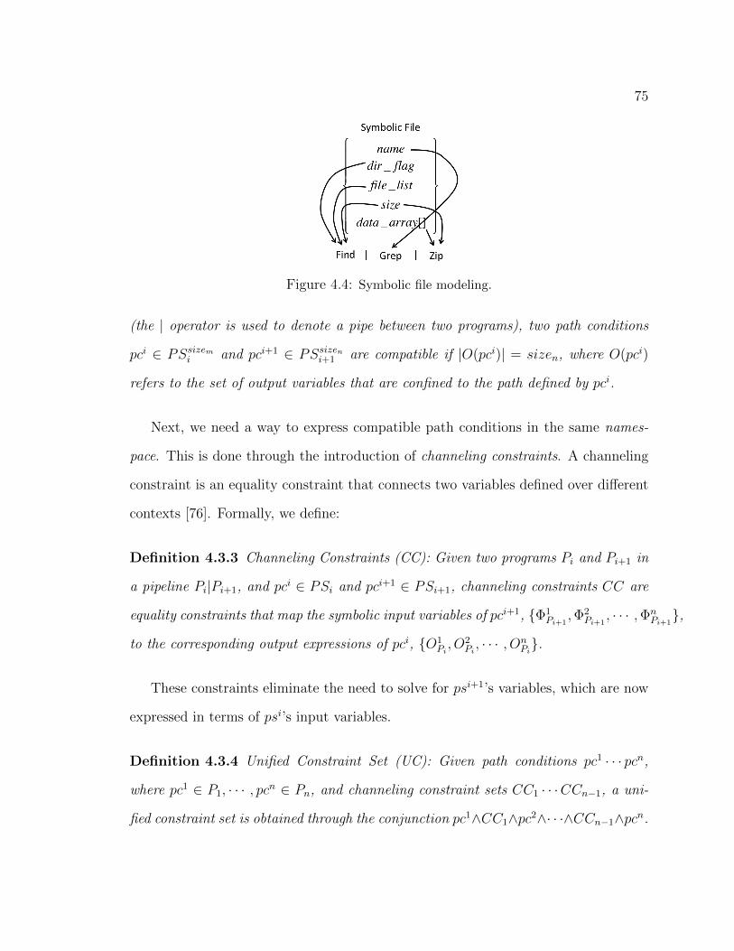
75

Figure 4.4: Symbolic file modeling.

(the | operator is used to denote a pipe between two programs), two path conditions

pci ∈ PSsizemi and pci+1 ∈ PSsizen

i+1 are compatible if |O(pci)| = sizen, where O(pci)

refers to the set of output variables that are confined to the path defined by pci.

Next, we need a way to express compatible path conditions in the same names-

pace. This is done through the introduction of channeling constraints. A channeling

constraint is an equality constraint that connects two variables defined over different

contexts [76]. Formally, we define:

Definition 4.3.3 Channeling Constraints (CC): Given two programs Pi and Pi+1 in

a pipeline Pi|Pi+1, and pci ∈ PSi and pci+1 ∈ PSi+1, channeling constraints CC are

equality constraints that map the symbolic input variables of pci+1, {Φ1Pi+1

,Φ2Pi+1

, · · · ,ΦnPi+1},

to the corresponding output expressions of pci, {O1Pi, O2

Pi, · · · , On

Pi}.

These constraints eliminate the need to solve for psi+1’s variables, which are now

expressed in terms of psi’s input variables.

Definition 4.3.4 Unified Constraint Set (UC): Given path conditions pc1 · · · pcn,

where pc1 ∈ P1, · · · , pcn ∈ Pn, and channeling constraint sets CC1 · · ·CCn−1, a uni-

fied constraint set is obtained through the conjunction pc1∧CC1∧pc2∧· · ·∧CCn−1∧pcn.

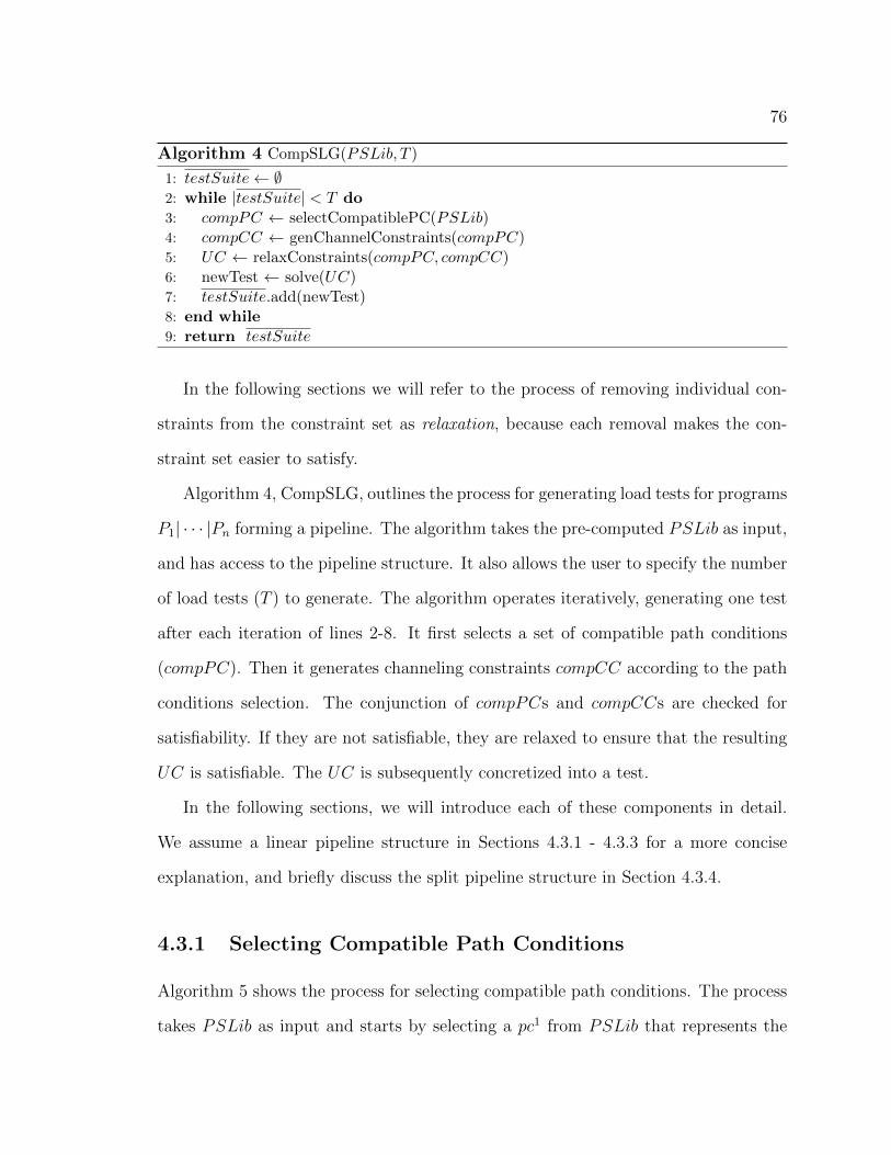
76

Algorithm 4 CompSLG(PSLib, T )

1: testSuite← ∅2: while |testSuite| < T do3: compPC ← selectCompatiblePC(PSLib)4: compCC ← genChannelConstraints(compPC)5: UC ← relaxConstraints(compPC, compCC)6: newTest ← solve(UC)7: testSuite.add(newTest)8: end while9: return testSuite

In the following sections we will refer to the process of removing individual con-

straints from the constraint set as relaxation, because each removal makes the con-

straint set easier to satisfy.

Algorithm 4, CompSLG, outlines the process for generating load tests for programs

P1| · · · |Pn forming a pipeline. The algorithm takes the pre-computed PSLib as input,

and has access to the pipeline structure. It also allows the user to specify the number

of load tests (T ) to generate. The algorithm operates iteratively, generating one test

after each iteration of lines 2-8. It first selects a set of compatible path conditions

(compPC). Then it generates channeling constraints compCC according to the path

conditions selection. The conjunction of compPCs and compCCs are checked for

satisfiability. If they are not satisfiable, they are relaxed to ensure that the resulting

UC is satisfiable. The UC is subsequently concretized into a test.

In the following sections, we will introduce each of these components in detail.

We assume a linear pipeline structure in Sections 4.3.1 - 4.3.3 for a more concise

explanation, and briefly discuss the split pipeline structure in Section 4.3.4.

4.3.1 Selecting Compatible Path Conditions

Algorithm 5 shows the process for selecting compatible path conditions. The process

takes PSLib as input and starts by selecting a pc1 from PSLib that represents the

77

Algorithm 5 selectCompatiblePC(PSLib)

1: compPC ← ∅2: pc1worst ← worst-case(PSLib[PS1])3: compPC.add(pc1worst)4: PSLib.remove(pc1worst)5: for i ∈ (2, n) do6: pci ← worst-compatible(PSLib[PSi], pc

i−1)7: if pci 6= null then8: PSLib.remove(pci)9: else

10: pci ← SLG(Pi, |Oi|)11: if pci = null then12: message(“Cannot generate compatible summary for Pi”)13: break14: end if15: end if16: compPC.add(pci)17: end for18: return compPC

worst case for P1 (the first component of the pipeline). Then, the process examines

the output size associated with pc1 and finds a pc2 from the summaries of P2 with

a matching input size at Line 6 of Algorithm 5. The function worst-compatible

will find a match for pc2, and if multiple summaries are matched, it will select the

one with a higher weight score first. The process operates in this way to find for

each pci−1 a matching pci. This process continues until all programs have selected

compatible pcs. If CompSLG cannot find a compatible pc for a program, it will call

the SLG to generate one with the desired attributes, or stop if no such summary can

be generated.

Note that we start the selection of compatible paths conditions with the first

component of the pipeline and move forward matching pci−1 to pci so that, if a

compatible pci cannot be found, the approach can instruct SLG on the input size to

use to produce a compatible load test.

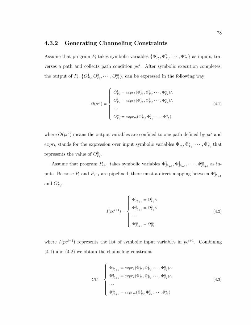
78

4.3.2 Generating Channeling Constraints

Assume that program Pi takes symbolic variables {Φ1Pi,Φ2

Pi, · · · ,Φn

Pi} as inputs, tra-

verses a path and collects path condition pci. After symbolic execution completes,

the output of Pi, {O1Pi, O2

Pi, · · · , Om

Pi}, can be expressed in the following way

O(pci) =

O1Pi

= expr1(Φ1Pi,Φ2

Pi, · · · ,Φn

Pi)∧

O2Pi

= expr2(Φ1Pi,Φ2

Pi, · · · ,Φn

Pi)∧

· · ·

OmPi

= exprm(Φ1Pi,Φ2

Pi, · · · ,Φn

Pi)

(4.1)

where O(pci) means the output variables are confined to one path defined by pci and

exprk stands for the expression over input symbolic variables Φ1Pi,Φ2

Pi, · · · ,Φn

Pithat

represents the value of OkPi

.

Assume that program Pi+1 takes symbolic variables Φ1Pi+1

,Φ2Pi+1

, · · · ,ΦmPi+1

as in-

puts. Because Pi and Pi+1 are pipelined, there must a direct mapping between ΦkPi+1

and OkPi

,

I(pci+1) =

Φ1Pi+1

= O1Pi∧

Φ2Pi+1

= O2Pi∧

· · ·

ΦmPi+1

= OmPi

(4.2)

where I(pci+1) represents the list of symbolic input variables in pci+1. Combining

(4.1) and (4.2) we obtain the channeling constraint

CC =

Φ1Pi+1

= expr1(Φ1Pi,Φ2

Pi, · · · ,Φn

Pi)∧

Φ2Pi+1

= expr2(Φ1Pi,Φ2

Pi, · · · ,Φn

Pi)∧

· · ·

ΦmPi+1

= exprm(Φ1Pi,Φ2

Pi, · · · ,Φn

Pi)

(4.3)

79

Algorithm 6 relaxConstraints(compPC, compCC)

1: UC ← union(compPC, compCC)2: while ¬ satisfiable(UC) do3: core ← computeUnsatCore(UC)4: c ← selectWeakestConstraint(core, compPC)5: removeConstraint(c, UC)6: end while7: return UC

Algorithm 7 selectWeakestConstraint(core, compPC)

1: for all c ∈ core do2: if c ∈ compPC then3: mark(c)4: end if5: end for6: targetPC ← lowestWeight(compPC)7: c ← marked(leastCost(targetPC))8: adjustWeight(targetPC)9: return c

For a linear pipeline there is one CC between each pair of path conditions. CC

allows for all constraints to be expressed in terms of Pi’s symbolic variables.

4.3.3 Weighing and Relaxing Constraints

If the set of generated constraints is not solvable, then the approach will sys-

tematically remove a constraint until it becomes solvable. During each iteration the

approach computes an unsatisfiable core of the constraint system under consideration,

and then removes one constraint that 1) appears in the unsatisfiable core, 2) appears

in the pc that has the least weight among all pcs, and 3) makes the least contribution

to the weight of that pc.

Algorithm 6 shows the procedure for weighing and relaxing constraints on compPC

collected over a set of linearly piped programs and the corresponding channeling con-

straints compCC. The algorithm starts by performing a conjunction of compPC and

80

compCC into a unified constraint set and tests for satisfiability. If UC is satisfied,

there is no need to relax constraints and the algorithm exits. Otherwise, the algorithm

repeatedly follows a three-step relaxation process (lines 2-6) until UC is satisfied.

First, an unsatisfiable core4 of UC is computed. Then the constraint c ∈ core,

deemed the weakest in terms of its impact on the load of the system, is removed from

UC. In the worst case, UC will be reduced to containing only the constraint from

one program, at which time it will be satisfiable because a PSi contains only feasible

paths.

Algorithm 7 details the subroutine for selecting the constraint of the least weight.

First, the unsatisfiable core and compPC are cross compared and constraints that

appear in both sets are marked on compPC (Lines 1-5). The algorithm then examines

the weight score on each pci and selects the one with the lowest weight(targetPC).

If there are more than one pci with the same lowest weight, the algorithm will pick

one randomly. The algorithm then selects the constraint c that is both marked and

has the lowest cost in targetPC and returns c (the cost of a constraint c is defined

as the difference in the weight of the pc before and after removing c).

Before returning, the weight score for the targetPC must be adjusted (Algo-

rithm 7 - line 8). This step is to ensure that past relaxations have an impact on

the current selection of the weakest constraint, so that we do not keep relaxing the

same pc. Therefore, the algorithm compensates the weight score for the pci whose con-

straint is relaxed at the current iteration. For pc1 · · · pcn with associated weight scores

w1 · · ·wn, after the relaxation of c ∈ pci, we compensate wi by a value determined by

w1 · · ·wn. One possible function we later explore is max{w1, w2, · · · , wn}/wi, where

4An unsatisfiable core is a subset of UC which preserves the unsatisfiability but is simplified.A minimum unsatisfiable core ensures that removing any one constraint breaks the unsatisfiability,while a minimal core is the smallest of minimum cores. Here a core is not guaranteed to be eitherminimum or minimal. As noted in a paper by Liffiton et al. [78], computing such a core is expensiveand no practical solver attempts to do so.

81

Table 4.5: Illustration of weighing and relaxing constraints. White areas correspond to theoriginal weight, shaded areas correspond to the adjusted weights.

Before Relaxation After 1st Relaxation

Grep 58 0Sort 15 0

0,

10,

20,

30,

40,

50,

60,

70,

Grep, Sort,Weight'

#'Conjuncts:'55'Weight:' '58'

#'Conjuncts:'28'Weight:' '15'

Grep 58 0Sort 14.5 4

0.

10.

20.

30.

40.

50.

60.

70.

Grep. Sort.

#"Conjuncts:"55"Weight:" "58"

#"Conjuncts:"27"Weight:"

1560.5+3.9=18.4"

Weight"

Starting to Relax Grep End of Relaxation

Grep 58 0Sort 8.03 52

0.

10.

20.

30.

40.

50.

60.

70.

Grep. Sort.

#"Conjuncts:"15"Weight:" "60.3"

Weight"

#"Conjuncts:"55"Weight:" "58"

Grep 56 2Sort 8.03 52

0/

10/

20/

30/

40/

50/

60/

70/

Grep/ Sort/


Weight"


the compensation is determined by wi’s ratio to the largest weight score.

Table 4.5 illustrates the process of weighing and relaxing of constraints on the run-

ning example. The weight scores are shown as bars on the graph, with the white area

indicating the original weight, and the shaded area indicating the adjusted weights.

The sum of weights and the number of remaining constraints are also listed at the

top of each bar. We can observe that before relaxation, the original weight scores are

58 for grep and 15 for sort. After removing the first constraint on sort (which has

a lower weight), its weight score is decreased by 0.5 due to the relaxation (remov-

ing the constraint made the path less costly), and increased by 58/15 = 3.9 due to

compensation (so the chances of selecting a constraint from sort in the future is less

82

likely). The third cell shows the turning point where after removing 13 constraints,

the weight on sort has been compensated enough to exceed that of grep, whose

constraints are starting to be removed. The fourth cell shows the weight scores at

the end of relaxation, with sort having 13 constraints removed, and grep having 2,

at which time UC becomes satisfiable.

4.3.4 Handling Split Pipelines

A split pipeline, in which the output of Pj is fed simultaneously to Pj+1, · · · , Pj+n,

can be viewed as a set of parallel linear pipelines Pj|Pj+1, · · · , Pj|Pj+n. Therefore,

we will solve split pipelines in a similar way as presented in Algorithms 4 - 7, with

a few modifications. Because in split pipelines, multiple components may share the

same predecessor (the splitting component), we need to add a queue data structure

at Line 6 of Algorithm 5 to identify the target component on which to invoke worst-

compatible.

We will discuss more complex structures beyond the realm of pipelines in Sec-

tion 4.6.

4.4 Implementation

We now discuss the most relevant implementation details of our CompSLG test gen-

erator and the support needed to handle the symbolic file system for Unix programs

that take a file as input.

CompSLG . CompSLG was implemented on top of SLG (Chapter 3). We build

the performance summary libraries by repeatedly invoking SLG on each component

of a pipeline. The summaries are stored in XML format. The channeling constraints

83

are computed by implementing a JPF listener that monitors write instructions for

the output variables, and traces their symbolic expressions from the stored system

states. We use Yices [131] to compute the unsatisfiable core during the constraint

weighing and relaxation. We first transform the constraints to a Yices compatible

format, and feed it to the solver. Should the solver return unsatisfiable, we then use

the yices get unsat core API to get the unsatisfiable core of the constraint set.

Symbolic File System Modeling . Certain Unix programs, such as Find, take a

file directory and a file property as inputs, and browse the directory for files matching

such a property. To enable symbolic execution of this type of command, we need to

treat the file system symbolically. We implemented several JPF interfaces to handle

most file system operations. For each file system operation (e.g. open), we check if

the action is for a concrete or a symbolic file. For concrete files, we simply invoke the

corresponding system call. For symbolic files we emulate the operation with symbolic

values (e.g. for open, we will return a file handler pointing to a symbolic file with all

fields declared as symbolic; for read, we will return symbolic bytes of the same size as

a concrete read would return). Users can specify size constraints on the symbolic file

system being used as inputs. The two size constraints are the number of file objects

(files or directories), and the overall size of these files. A symbolic file system can

contain as many levels of directories and as many files as desired, catering to the

current analysis progress, as long as the two size constraints are not violated.

4.5 Evaluation

We evaluate the cost and effectiveness of CompSLG relative to SLG and Random

approaches on various artifacts.

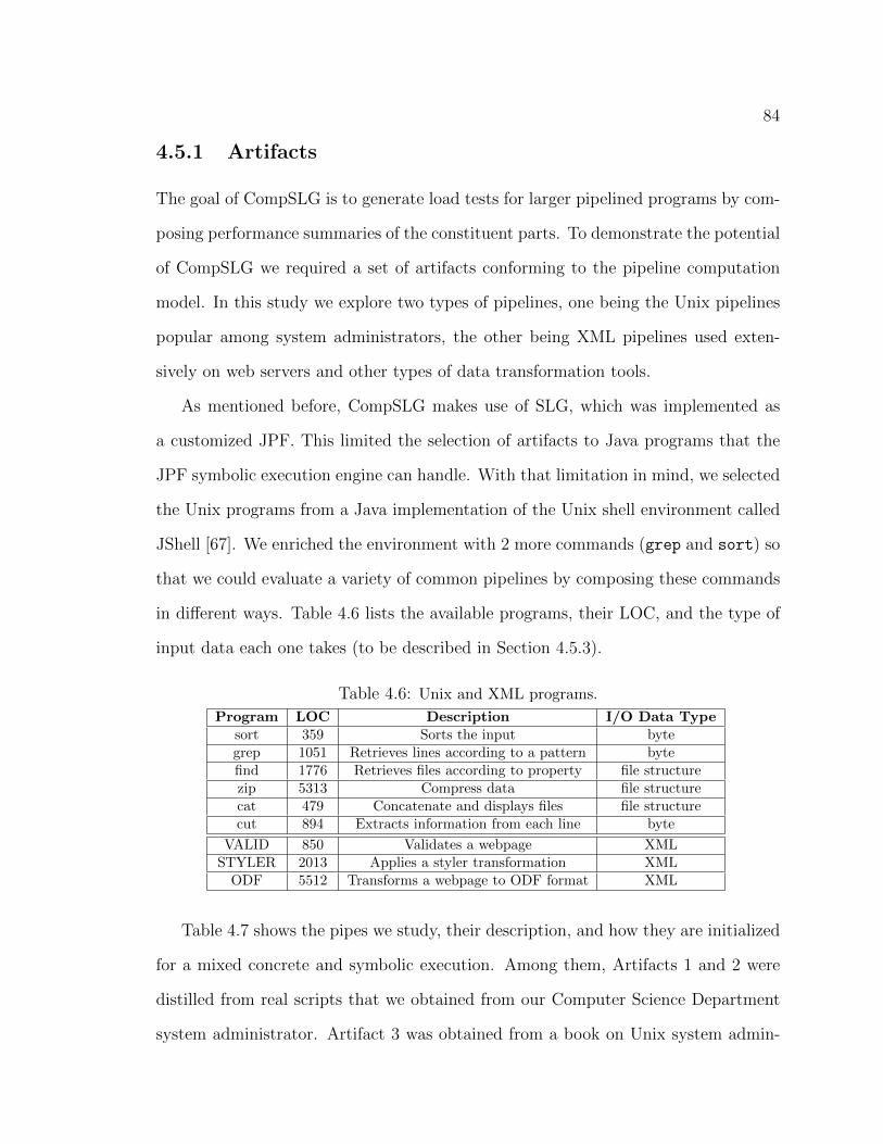
84

4.5.1 Artifacts

The goal of CompSLG is to generate load tests for larger pipelined programs by com-

posing performance summaries of the constituent parts. To demonstrate the potential

of CompSLG we required a set of artifacts conforming to the pipeline computation

model. In this study we explore two types of pipelines, one being the Unix pipelines

popular among system administrators, the other being XML pipelines used exten-

sively on web servers and other types of data transformation tools.

As mentioned before, CompSLG makes use of SLG, which was implemented as

a customized JPF. This limited the selection of artifacts to Java programs that the

JPF symbolic execution engine can handle. With that limitation in mind, we selected

the Unix programs from a Java implementation of the Unix shell environment called

JShell [67]. We enriched the environment with 2 more commands (grep and sort) so

that we could evaluate a variety of common pipelines by composing these commands

in different ways. Table 4.6 lists the available programs, their LOC, and the type of

input data each one takes (to be described in Section 4.5.3).

Table 4.6: Unix and XML programs.

Program LOC Description I/O Data Typesort 359 Sorts the input bytegrep 1051 Retrieves lines according to a pattern bytefind 1776 Retrieves files according to property file structurezip 5313 Compress data file structurecat 479 Concatenate and displays files file structurecut 894 Extracts information from each line byte

VALID 850 Validates a webpage XMLSTYLER 2013 Applies a styler transformation XML

ODF 5512 Transforms a webpage to ODF format XML

Table 4.7 shows the pipes we study, their description, and how they are initialized

for a mixed concrete and symbolic execution. Among them, Artifacts 1 and 2 were

distilled from real scripts that we obtained from our Computer Science Department

system administrator. Artifact 3 was obtained from a book on Unix system admin-

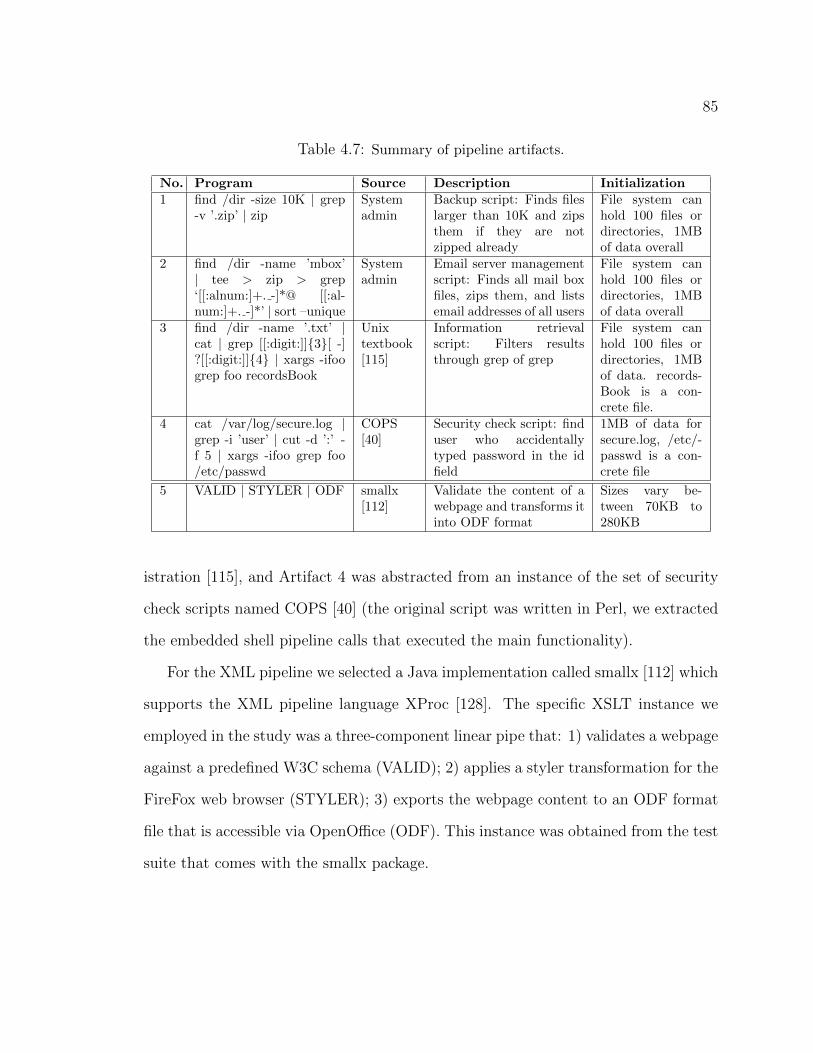
85

Table 4.7: Summary of pipeline artifacts.

No. Program Source Description Initialization1 find /dir -size 10K | grep

-v ’.zip’ | zipSystemadmin

Backup script: Finds fileslarger than 10K and zipsthem if they are notzipped already

File system canhold 100 files ordirectories, 1MBof data overall

2 find /dir -name ’mbox’| tee > zip > grep‘[[:alnum:]+. -]*@ [[:al-num:]+. -]*’ | sort –unique

Systemadmin

Email server managementscript: Finds all mail boxfiles, zips them, and listsemail addresses of all users

File system canhold 100 files ordirectories, 1MBof data overall

3 find /dir -name ’.txt’ |cat | grep [[:digit:]]{3}[ -]?[[:digit:]]{4} | xargs -ifoogrep foo recordsBook

Unixtextbook[115]

Information retrievalscript: Filters resultsthrough grep of grep

File system canhold 100 files ordirectories, 1MBof data. records-Book is a con-crete file.

4 cat /var/log/secure.log |grep -i ’user’ | cut -d ’:’ -f 5 | xargs -ifoo grep foo/etc/passwd

COPS[40]

Security check script: finduser who accidentallytyped password in the idfield

1MB of data forsecure.log, /etc/-passwd is a con-crete file

5 VALID | STYLER | ODF smallx[112]

Validate the content of awebpage and transforms itinto ODF format

Sizes vary be-tween 70KB to280KB

istration [115], and Artifact 4 was abstracted from an instance of the set of security

check scripts named COPS [40] (the original script was written in Perl, we extracted

the embedded shell pipeline calls that executed the main functionality).

For the XML pipeline we selected a Java implementation called smallx [112] which

supports the XML pipeline language XProc [128]. The specific XSLT instance we

employed in the study was a three-component linear pipe that: 1) validates a webpage

against a predefined W3C schema (VALID); 2) applies a styler transformation for the

FireFox web browser (STYLER); 3) exports the webpage content to an ODF format

file that is accessible via OpenOffice (ODF). This instance was obtained from the test

suite that comes with the smallx package.

86

4.5.2 Metrics and Treatments

We assess the effectiveness of a load test by measuring its effect on the response time

of the target program. We measure costs in terms of the time necessary for the

approach to generate a test suite.

The main treatment in the study is the CompSLG approach as described in Section

4.3. We study three variants of CompSLG, described as follows:

• No-reuse: all performance summaries are generated for each artifact on the

fly, with no reuse of summaries among artifacts.

• Incremental-reuse: the artifacts are analyzed in the order defined in Table 4.6,

and summaries are reused when possible. For example, Artifact 2 could reuse

the summary generated for find in Artifact 1 because they both use the same

command and they were invoked with the same input constraints.

• Full-reuse: assumes that all summaries were collected previously, so the gen-

eration cost only corresponds to the composition effort.

We use two control treatments, SLG and random test generation. SLG is selected

as an alternative symbolic load generation approach and Random is used to provide

a baseline comparison. For SLG, we apply it to the whole pipeline by treating it as

a single program, and we apply it to each component of the pipeline independently,

which will reduce the analysis burden, but sacrifices effectiveness in generating a load

for the whole pipeline.

For the Random treatment, we treat the pipeline as a single program and we

randomly generate one type of input that feeds into the first component. We adopt

a generate-and-run scheme for retaining the most effective tests as they are being

generated. Random is run for as long as the compositional approach to enable a

comparison with the same baseline cost.

87

We generate 10 tests for all treatments and report average measures of the 10.

4.5.3 Experiment Setup

For Unix pipelines taking a file system as input (e.g., via the find command), we

initialize it with a symbolic file system and constrain the total number of files and

directories it can access. For pipelines taking a single file as input, we simply constrain

the size of that file. In Table 4.7, column “Initialization” specifies the size constraints

we use for the analysis on the Unix pipelines.

For the XML pipeline, we select an input size of 140K, which is reported to be the

average size of webpages that exist on the Internet [123]. To explore how CompSLG

performs with various input sizes, we also generate tests for two more input sizes,

which are 50% and 200% of 140K. In addition to input sizes, we also impose a set of

structural constraints on the input to the XML pipeline program. We specify that the

input webpage can contain six types of tags (paragraph, heading, hyperlink, image,

list, and table tags), and that each of those tags has an upper count of 160 (the

associated test suite of smallx uses six types of tags and the maximum usage count of

a tag is 160. We use the same settings in our experiment). This set of constraints is

to ensure that the approach is not stuck in a local optimum, and the resulting tests

are more diverse.

We use SLG as a subroutine for the main treatment (as described in Section 4.4)

and as a standalone control treatment. We use the same SLG configuration as in

previous empirical studies (Section 3.5), with iterative searches of 50 branches in

length and maximum path size of 30000 in order to keep within the capabilities of

the various constraint solvers we used. We enforce a generation time cap of five hours

across all runs. If exceeded, the analysis is terminated and no results are reported.

Throughout the study we use the same platform for all programs, a 2.4 GHz Intel

88

Core 2 Duo machine with Mac OS X 10.6.7 and 4GB memory. We executed our tool

on the JVM 1.6 with 2GB of memory.

4.5.4 Results and Analysis

Figure 4.5 shows results on the Unix pipelines. Each figure corresponds to one artifact

specified in Table 4.7. The x-axis shows the cost of generating load tests measured in

terms of generation time in minutes, and the y-axis shows the effectiveness of running

those tests, measured in terms of the average response time in seconds, induced

by the 10 tests produced by each treatment. On each figure we plot three sets of

data points corresponding to the three treatments used in the study. The triangles

refer to CompSLG, with white triangles indicating No-reuse, grey triangles indicating

Incremental-reuse, and black triangles indicating Full-reuse; the diamonds refer to the

SLG treatment applied to a program in the pipeline to generate input for the whole

pipeline, and the circles refer to the Random treatment, with colors matched to each

variation of CompSLG. Figure 4.6 shows the results on the XML pipeline in the same

format.

We first applied SLG on the whole pipelines and found that none of them could

finish within five hours, so they were terminated and are not depicted in the figures.

For the rest of the treatments, we describe our findings in terms of effectiveness first

and then cost.

We notice that the various types of CompSLG are all capable of inducing more

load than the other treatments across all artifacts. CompSLG produces load tests

that generate as much as 4.4X times more load than Random on a Unix pipeline

(Artifact 4), and as much as 2.8X on the XML pipeline (280K) with the same cost.

We also note that the three variants of CompSLG show almost no variance in terms

of effectiveness, indicating that reuse of previously computed summaries does not de-

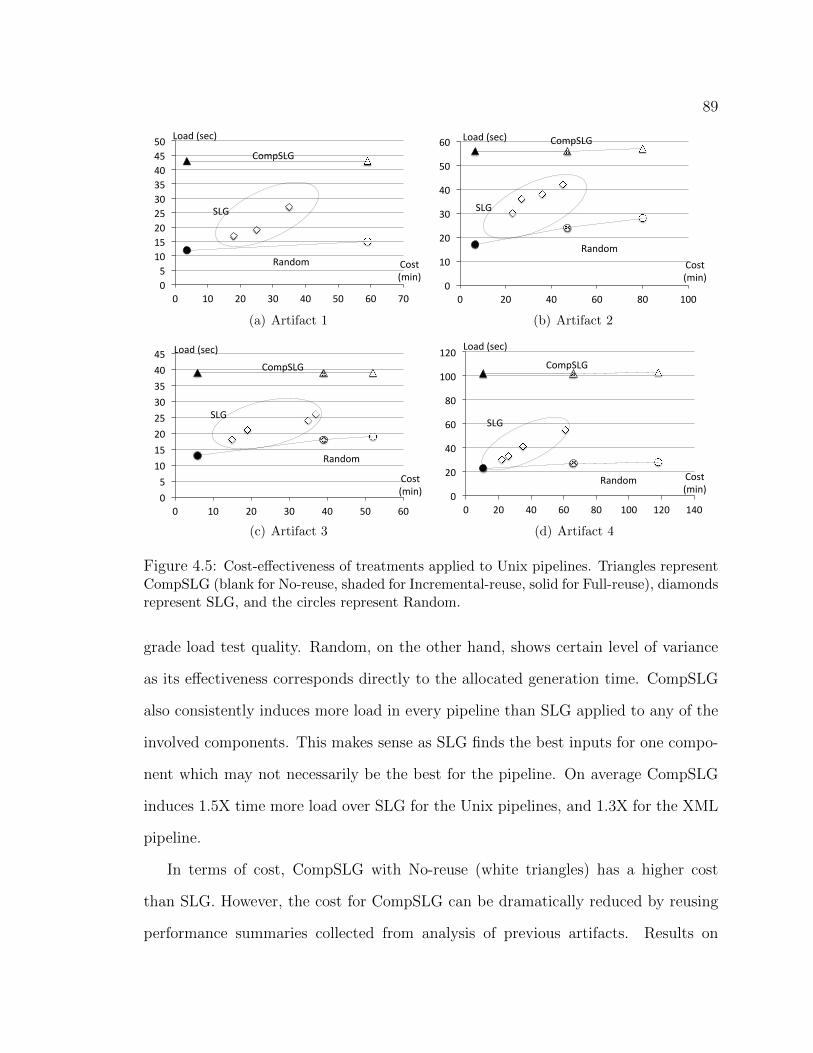
89

random 59 15 59 43 59 15SLG 18 17 59 43 3.6 12SLG 25 19 3.6 43SLG 35 27SLGRandom2 3.6 12

0656106156206256306356406456506

06 106 206 306 406 506 606 706

SLG6

CompSLG6

Cost6(min)6

Load6(sec)6

Random6

(a) Artifact 1

random 80 28 80 57 80 28SLG 23 30 47 56 47 24SLG 36 38 6.6 56 6.6 17SLG 45 42SLG 27 36compSymb 59 43

09

109

209

309

409

509

609

09 209 409 609 809 1009

SLG9

CompSLG9

Cost9(min)9

Load9(sec)9

Random9

(b) Artifact 2


0959109159209259309359409459

09 109 209 309 409 509 609

SLG9

CompSLG9

Cost9(min)9

Load9(sec)9

Random9

(c) Artifact 3


08

208

408

608

808

1008

1208

08 208 408 608 808 1008 1208 1408

SLG8

CompSLG8

Cost8(min)8

Load8(sec)8

Random8

(d) Artifact 4

Figure 4.5: Cost-effectiveness of treatments applied to Unix pipelines. Triangles representCompSLG (blank for No-reuse, shaded for Incremental-reuse, solid for Full-reuse), diamondsrepresent SLG, and the circles represent Random.

grade load test quality. Random, on the other hand, shows certain level of variance

as its effectiveness corresponds directly to the allocated generation time. CompSLG

also consistently induces more load in every pipeline than SLG applied to any of the

involved components. This makes sense as SLG finds the best inputs for one compo-

nent which may not necessarily be the best for the pipeline. On average CompSLG

induces 1.5X time more load over SLG for the Unix pipelines, and 1.3X for the XML

pipeline.

In terms of cost, CompSLG with No-reuse (white triangles) has a higher cost

than SLG. However, the cost for CompSLG can be dramatically reduced by reusing

performance summaries collected from analysis of previous artifacts. Results on

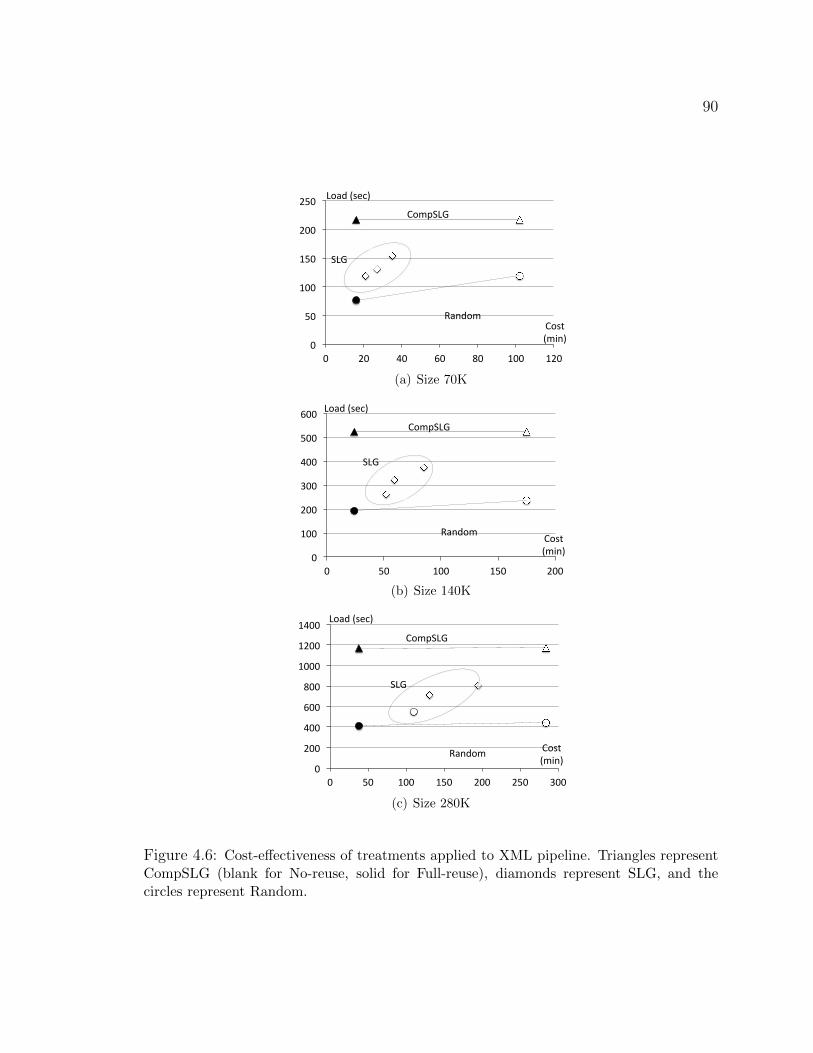
90

random 102 119 102 217 102 119SLG 21 119 16 217 16 77SLG 27 131SLG 35 154SLGcompSymb 102 217

07

507

1007

1507

2007

2507

07 207 407 607 807 1007 1207

SLG7

CompSLG7

Cost7(min)7

Load7(sec)7

Random7

(a) Size 70K


08

1008

2008

3008

4008

5008

6008

08 508 1008 1508 2008

SLG8

CompSLG8

Cost8(min)8

Load8(sec)8

Random8

(b) Size 140K


08

2008

4008

6008

8008

10008

12008

14008

08 508 1008 1508 2008 2508 3008

SLG8

CompSLG8

Cost8(min)8

Load8(sec)8

Random8

(c) Size 280K

Figure 4.6: Cost-effectiveness of treatments applied to XML pipeline. Triangles representCompSLG (blank for No-reuse, solid for Full-reuse), diamonds represent SLG, and thecircles represent Random.

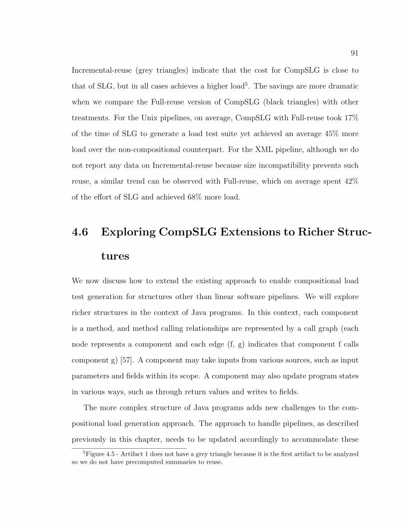
91

Incremental-reuse (grey triangles) indicate that the cost for CompSLG is close to

that of SLG, but in all cases achieves a higher load5. The savings are more dramatic

when we compare the Full-reuse version of CompSLG (black triangles) with other

treatments. For the Unix pipelines, on average, CompSLG with Full-reuse took 17%

of the time of SLG to generate a load test suite yet achieved an average 45% more

load over the non-compositional counterpart. For the XML pipeline, although we do

not report any data on Incremental-reuse because size incompatibility prevents such

reuse, a similar trend can be observed with Full-reuse, which on average spent 42%

of the effort of SLG and achieved 68% more load.

4.6 Exploring CompSLG Extensions to Richer Struc-

tures

We now discuss how to extend the existing approach to enable compositional load

test generation for structures other than linear software pipelines. We will explore

richer structures in the context of Java programs. In this context, each component

is a method, and method calling relationships are represented by a call graph (each

node represents a component and each edge (f, g) indicates that component f calls

component g) [57]. A component may take inputs from various sources, such as input

parameters and fields within its scope. A component may also update program states

in various ways, such as through return values and writes to fields.

The more complex structure of Java programs adds new challenges to the com-

positional load generation approach. The approach to handle pipelines, as described

previously in this chapter, needs to be updated accordingly to accommodate these

5Figure 4.5 - Artifact 1 does not have a grey triangle because it is the first artifact to be analyzedso we do not have precomputed summaries to reuse.

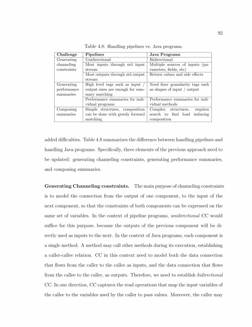
92

Table 4.8: Handling pipelines vs. Java programs.

Challenge Pipelines Java ProgramsGeneratingchannelingconstraints

Unidirectional BidirectionalMost inputs through std inputstream

Multiple sources of inputs (pa-rameters, fields, etc)

Most outputs through std outputstream

Return values and side effects

Generatingperformancesummaries

High level tags such as input /output sizes are enough for sum-mary matching

Need finer granularity tags suchas shapes of input / output

Performance summaries for indi-vidual programs

Performance summaries for indi-vidual methods

Composingsummaries

Simple structures, compositioncan be done with greedy forwardmatching

Complex structures, requiressearch to find load inducingcomposition

added difficulties. Table 4.8 summarizes the difference between handling pipelines and

handling Java programs. Specifically, three elements of the previous approach need to

be updated: generating channeling constraints, generating performance summaries,

and composing summaries.

Generating Channeling constraints. The main purpose of channeling constraints

is to model the connection from the output of one component, to the input of the

next component, so that the constraints of both components can be expressed on the

same set of variables. In the context of pipeline programs, unidirectional CC would

suffice for this purpose, because the outputs of the previous component will be di-

rectly used as inputs to the next. In the context of Java programs, each component is

a single method. A method may call other methods during its execution, establishing

a caller-callee relation. CC in this context need to model both the data connection

that flows from the caller to the callee as inputs, and the data connection that flows

from the callee to the caller, as outputs. Therefore, we need to establish bidirectional

CC. In one direction, CC captures the read operations that map the input variables of

the callee to the variables used by the caller to pass values. Moreover, the caller may

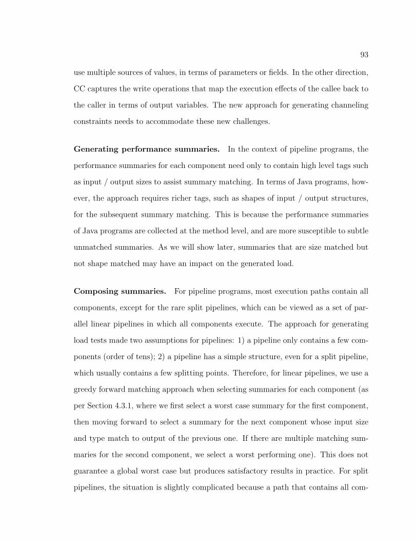
93

use multiple sources of values, in terms of parameters or fields. In the other direction,

CC captures the write operations that map the execution effects of the callee back to

the caller in terms of output variables. The new approach for generating channeling

constraints needs to accommodate these new challenges.

Generating performance summaries. In the context of pipeline programs, the

performance summaries for each component need only to contain high level tags such

as input / output sizes to assist summary matching. In terms of Java programs, how-

ever, the approach requires richer tags, such as shapes of input / output structures,

for the subsequent summary matching. This is because the performance summaries

of Java programs are collected at the method level, and are more susceptible to subtle

unmatched summaries. As we will show later, summaries that are size matched but

not shape matched may have an impact on the generated load.

Composing summaries. For pipeline programs, most execution paths contain all

components, except for the rare split pipelines, which can be viewed as a set of par-

allel linear pipelines in which all components execute. The approach for generating

load tests made two assumptions for pipelines: 1) a pipeline only contains a few com-

ponents (order of tens); 2) a pipeline has a simple structure, even for a split pipeline,

which usually contains a few splitting points. Therefore, for linear pipelines, we use a

greedy forward matching approach when selecting summaries for each component (as

per Section 4.3.1, where we first select a worst case summary for the first component,

then moving forward to select a summary for the next component whose input size

and type match to output of the previous one. If there are multiple matching sum-

maries for the second component, we select a worst performing one). This does not

guarantee a global worst case but produces satisfactory results in practice. For split

pipelines, the situation is slightly complicated because a path that contains all com-

94

ponents may not correspond to the worst case. However, because the split pipeline

only contains a few components and a simple structure, it is usually affordable to

explore all possible ways of component composition, then pick up the most expensive

one for test generation.

For Java programs, both assumptions do not hold anymore. First, the process

needs to select summaries for potentially hundreds of components, so a greedy for-

ward matching approach may be too shortsighted when doing so. The negative effects

of poorly selected summaries may aggregate in the structure, eventually lead to degra-

dation in induced load. Second, due to the complex structure of Java programs, it

is infeasible to traverse all possible ways of component composition to determine the

worst one.

4.6.1 Richer Channeling Constraints

The added complexity of Java programs calls for a more elaborate definition of the

channeling constraints. The new channeling constraints need to capture both the

connection that map the values at a call site to the input variables of the called

component, and the connection that maps the execution effect of the component

back to its call site. It also needs to handle multiple sources of inputs (parameters

and fields) and outputs (return values and side effects). We discuss these needs next.

4.6.1.1 Approach to Capture CCr and CCw

We start by redefining channeling constraints in the context of Java programs, then

present some implementation details and several proof-of-concept examples.

Definition 4.6.1 Channeling Constraints (CC): Given two components f and g in a

system, where f is called by g at call sites CSfg , and pcf , a performance summary of f ,

95

channeling constraints are equality constraints that map the symbolic input variables

of pcf to CSfg , so that pcf can be reused when computing a summary for g. For every

call site csfi , we define two sets of channeling constraints: 1) CCfir, which captures

the parameters and fields in the system that map to the symbolic input variables of

pcf through read operations. 2) CCfiw, which captures the execution effects of f back

to the corresponding variables in the system through write operations.

The new definition describes the bidirectional nature of the channeling constraints.

In one direction, CCfir maps the symbolic input variables of f to its various input

sources at its call site csfi . In the other direction, CCfiw maps the execution effects of

f back to call site csfi , ensuring that its effects, both in the form of return values and

side effects on the field variables, are accounted for.

As defined, CCfiw maps the execution effects of f back to the call site csfi . Because

the execution effects can be captured by symbolically executing f once, therefore

CCfiw can be generated during the collection of the performance summaries by SLG.

To apply CCfiw to specific call sites, we only need to substitute the generic names

of the output variables in CCfiw with the corresponding variable names at the call

site. Such symbolic execution may over-approximate program behaviors at certain

call sites, especially when f containing calls to unknown or complex functions, which

are treated as uninterpreted functions. In such case, CCfiw will also over-approximate

the execution effects of f . The process of generating CCfiw is similar to generating

CC for pipeline programs (as described in Section 4.3.2), except that for pipelines,

the output variables are the ones that are written to the standard i/o streams (pipes),

while in this case, the output variables are the return values and updates to the fields.

The process for generating CCfir is more complicated. Generally, CCf

ir maps the

symbolic input variables of f to its various input sources at csfi . Those input sources,

which are carried by variables of the caller, are passed to the callee in terms of

96

parameters or fields. To correctly capture CCfir, we need to ensure that all write

operations to those input variables up to csfi are accounted for by the analysis. For

the write operations that are performed by the caller, we need to use a customized

symbolic execution (Custom-SE) to generate summaries for those operations up to

a call site. The goal of the Custom-SE is to capture the write operations by the

caller to the variables that may be used as input sources to f at a particular csfi .

However, Custom-SE does not need to capture all write operations at the calling

context, as certain optimizations can be applied. First, when Custom-SE is called to

generate CCfir at csfi , it only needs to analyze the code segment in the caller from

the point the last callee returns to its call site, to csfi where f is being invoked. This

is because all behaviors up to the point of the last call return have already been

accounted for by previous analysis. For example, in the calling context of f , if csfi

has a predecessor csf′

i which invokes another component f ′, Custom-SE only needs

to analyze the code segment between the two call sites. Second, assuming that we

already have the performance summary of f from SLG, we can determine the types

of input variables, and capture write operations on those types only. For example, if

f takes only integers as its inputs, then in performing the Custom-SE, we only need

capture the write operations on integer variables.

Algorithm 8 illustrates the process of Custom-SE, which we adopt from a previous

work on using compositional symbolic execution to test software product lines [106].

The original version was used to compute the edge summaries for the common code

that various features interact with. It can be adopted to our needs, because features

in a SPL can be viewed as analogous to components in our context. We slightly

updated the original algorithm to capture only the write updates to the types of

data we are interested in, instead of capturing all writes (Line 14). The algorithm

makes use of several helper functions: branch() determines whether an instruction is

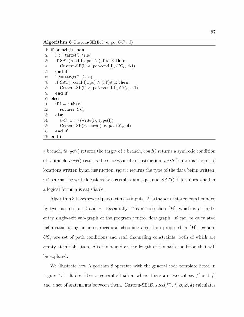
97

Algorithm 8 Custom-SE(E, l, e, pc, CCr, d)

1: if branch(l) then2: l’ := target(l, true)3: if SAT(cond(l)∪pc) ∧ (l,l’)∈ E then4: Custom-SE(l’, e, pc∧cond(l), CCr, d-1)5: end if6: l’ := target(l, false)7: if SAT(¬cond(l)∪pc) ∧ (l,l’)∈ E then8: Custom-SE(l’, e, pc∧¬cond(l), CCr, d-1)9: end if

10: else11: if l = e then12: return CCr

13: else14: CCr ∪= π(write(l), type(l))15: Custom-SE(E, succ(l), e, pc, CCr, d)16: end if17: end if

a branch, target() returns the target of a branch, cond() returns a symbolic condition

of a branch, succ() returns the successor of an instruction, write() returns the set of

locations written by an instruction, type() returns the type of the data being written,

π() screens the write locations by a certain data type, and SAT () determines whether

a logical formula is satisfiable.

Algorithm 8 takes several parameters as inputs. E is the set of statements bounded

by two instructions l and e. Essentially E is a code chop [94], which is a single-

entry single-exit sub-graph of the program control flow graph. E can be calculated

beforehand using an interprocedural chopping algorithm proposed in [94]. pc and

CCr are set of path conditions and read channeling constraints, both of which are

empty at initialization. d is the bound on the length of the path condition that will

be explored.

We illustrate how Algorithm 8 operates with the general code template listed in

Figure 4.7. It describes a general situation where there are two callees f ′ and f ,

and a set of statements between them. Custom-SE(E, succ(f ′), f,∅,∅, d) calculates

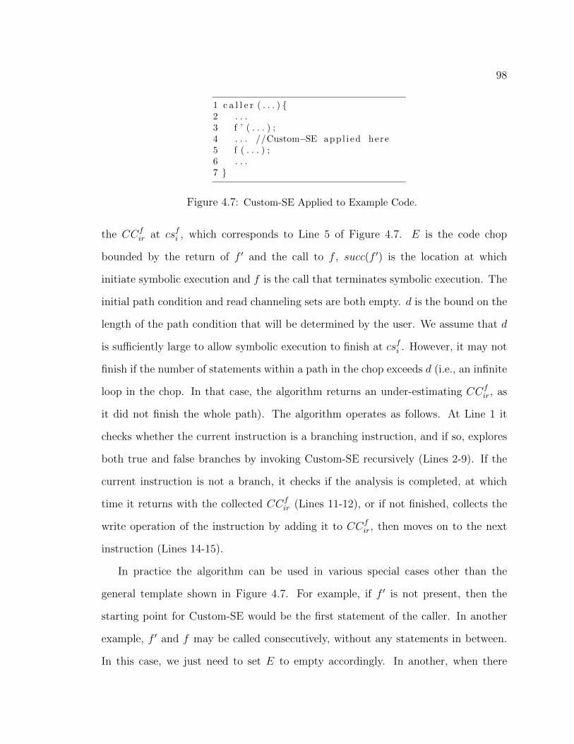
98

1 c a l l e r ( . . . ) {2 . . .3 f ’ ( . . . ) ;4 . . . //Custom−SE app l i ed here5 f ( . . . ) ;6 . . .7 }

Figure 4.7: Custom-SE Applied to Example Code.

the CCfir at csfi , which corresponds to Line 5 of Figure 4.7. E is the code chop

bounded by the return of f ′ and the call to f , succ(f ′) is the location at which

initiate symbolic execution and f is the call that terminates symbolic execution. The

initial path condition and read channeling sets are both empty. d is the bound on the

length of the path condition that will be determined by the user. We assume that d

is sufficiently large to allow symbolic execution to finish at csfi . However, it may not

finish if the number of statements within a path in the chop exceeds d (i.e., an infinite

loop in the chop. In that case, the algorithm returns an under-estimating CCfir, as

it did not finish the whole path). The algorithm operates as follows. At Line 1 it

checks whether the current instruction is a branching instruction, and if so, explores

both true and false branches by invoking Custom-SE recursively (Lines 2-9). If the

current instruction is not a branch, it checks if the analysis is completed, at which

time it returns with the collected CCfir (Lines 11-12), or if not finished, collects the

write operation of the instruction by adding it to CCfir, then moves on to the next

instruction (Lines 14-15).

In practice the algorithm can be used in various special cases other than the

general template shown in Figure 4.7. For example, if f ′ is not present, then the

starting point for Custom-SE would be the first statement of the caller. In another

example, f ′ and f may be called consecutively, without any statements in between.

In this case, we just need to set E to empty accordingly. In another, when there

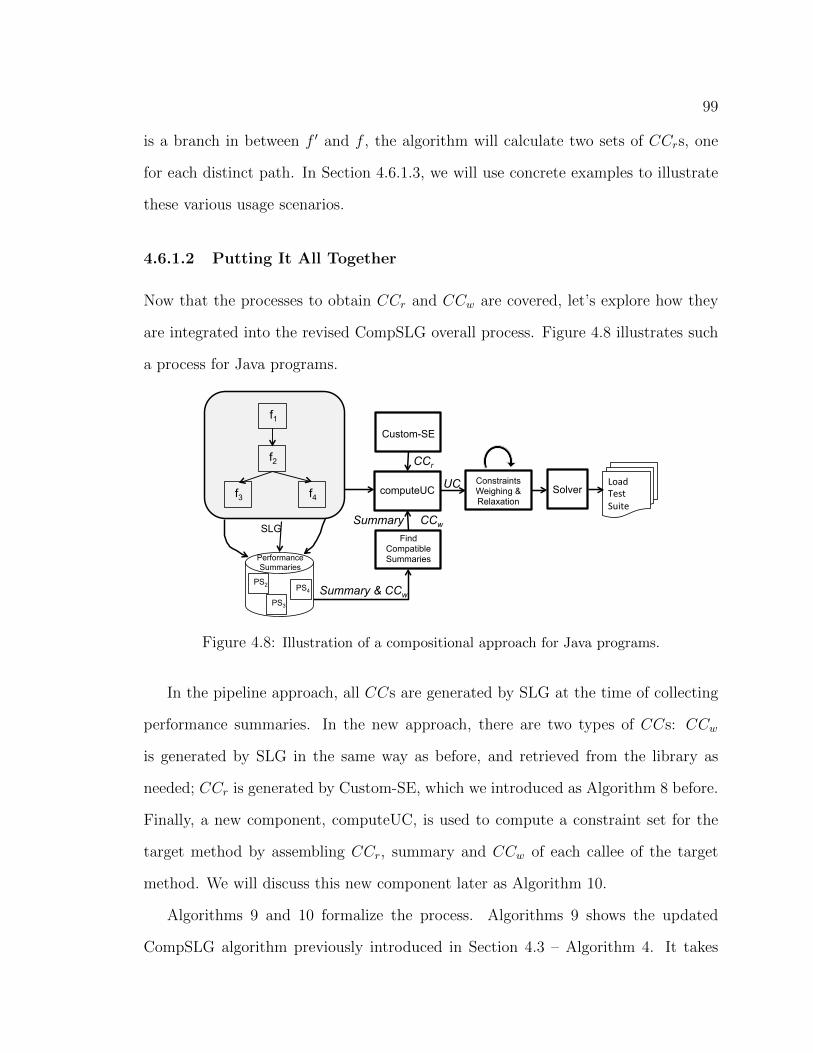
99

is a branch in between f ′ and f , the algorithm will calculate two sets of CCrs, one

for each distinct path. In Section 4.6.1.3, we will use concrete examples to illustrate

these various usage scenarios.

4.6.1.2 Putting It All Together

Now that the processes to obtain CCr and CCw are covered, let’s explore how they

are integrated into the revised CompSLG overall process. Figure 4.8 illustrates such

a process for Java programs.

Load Test Suite

Performance Summaries

PS2

PS3

PS4

Find Compatible Summaries

Constraints Weighing & Relaxation

Solver

SLG

f2

f1

f3 f4

Custom-SE

CCr

Summary & CCw

computeUC UC

Summary CCw

Figure 4.8: Illustration of a compositional approach for Java programs.

In the pipeline approach, all CCs are generated by SLG at the time of collecting

performance summaries. In the new approach, there are two types of CCs: CCw

is generated by SLG in the same way as before, and retrieved from the library as

needed; CCr is generated by Custom-SE, which we introduced as Algorithm 8 before.

Finally, a new component, computeUC, is used to compute a constraint set for the

target method by assembling CCr, summary and CCw of each callee of the target

method. We will discuss this new component later as Algorithm 10.

Algorithms 9 and 10 formalize the process. Algorithms 9 shows the updated

CompSLG algorithm previously introduced in Section 4.3 – Algorithm 4. It takes

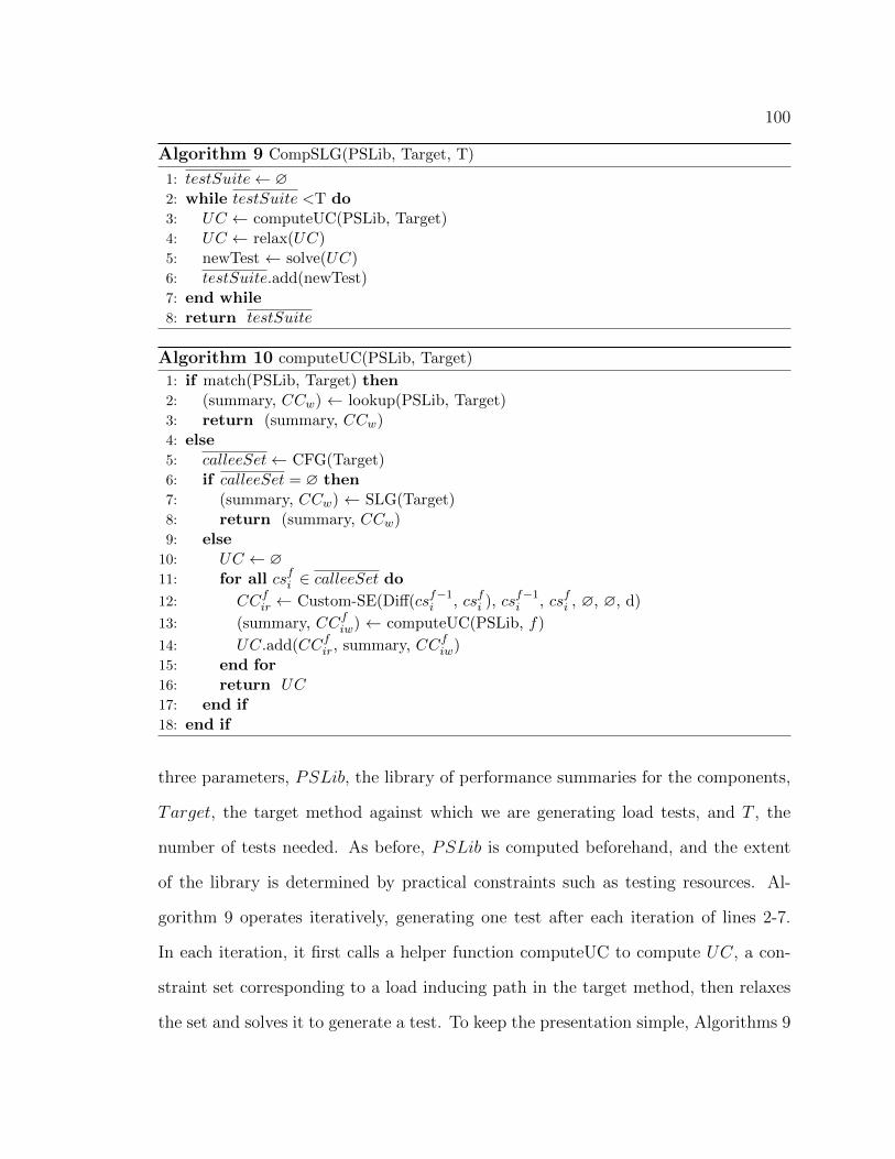
100

Algorithm 9 CompSLG(PSLib, Target, T)

1: testSuite← ∅2: while testSuite <T do3: UC ← computeUC(PSLib, Target)4: UC ← relax(UC)5: newTest ← solve(UC)6: testSuite.add(newTest)7: end while8: return testSuite

Algorithm 10 computeUC(PSLib, Target)

1: if match(PSLib, Target) then2: (summary, CCw) ← lookup(PSLib, Target)3: return (summary, CCw)4: else5: calleeSet← CFG(Target)6: if calleeSet = ∅ then7: (summary, CCw) ← SLG(Target)8: return (summary, CCw)9: else

10: UC ← ∅11: for all csfi ∈ calleeSet do

12: CCfir ← Custom-SE(Diff(csf−1i , csfi ), csf−1i , csfi , ∅, ∅, d)

13: (summary, CCfiw) ← computeUC(PSLib, f)

14: UC.add(CCfir, summary, CCf

iw)15: end for16: return UC17: end if18: end if

three parameters, PSLib, the library of performance summaries for the components,

Target, the target method against which we are generating load tests, and T , the

number of tests needed. As before, PSLib is computed beforehand, and the extent

of the library is determined by practical constraints such as testing resources. Al-

gorithm 9 operates iteratively, generating one test after each iteration of lines 2-7.

In each iteration, it first calls a helper function computeUC to compute UC, a con-

straint set corresponding to a load inducing path in the target method, then relaxes

the set and solves it to generate a test. To keep the presentation simple, Algorithms 9

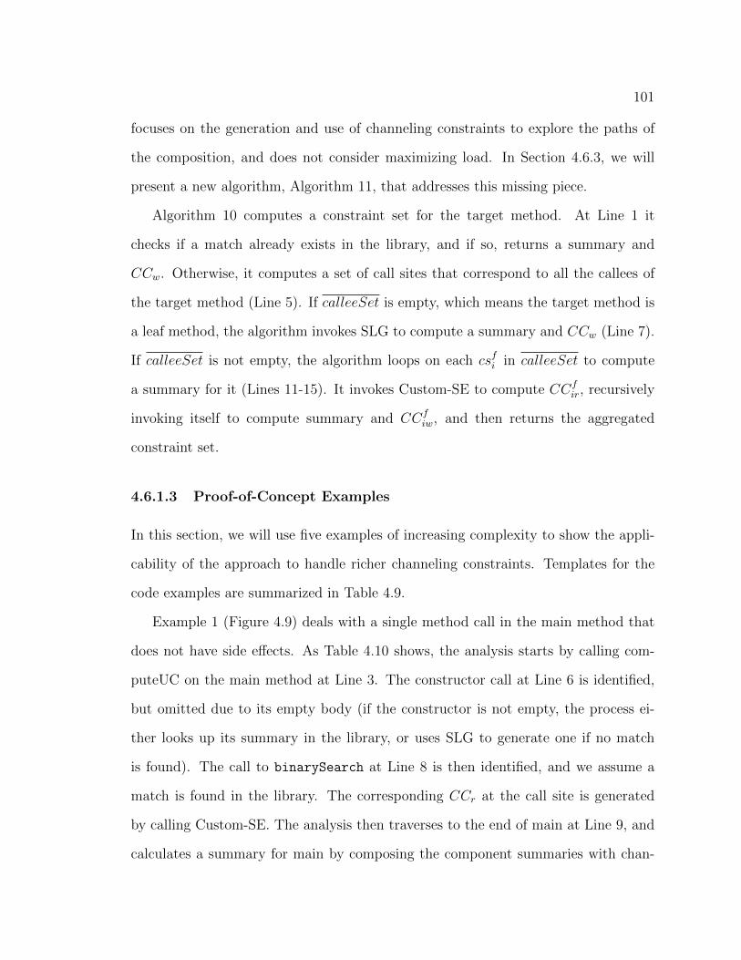
101

focuses on the generation and use of channeling constraints to explore the paths of

the composition, and does not consider maximizing load. In Section 4.6.3, we will

present a new algorithm, Algorithm 11, that addresses this missing piece.

Algorithm 10 computes a constraint set for the target method. At Line 1 it

checks if a match already exists in the library, and if so, returns a summary and

CCw. Otherwise, it computes a set of call sites that correspond to all the callees of

the target method (Line 5). If calleeSet is empty, which means the target method is

a leaf method, the algorithm invokes SLG to compute a summary and CCw (Line 7).

If calleeSet is not empty, the algorithm loops on each csfi in calleeSet to compute

a summary for it (Lines 11-15). It invokes Custom-SE to compute CCfir, recursively

invoking itself to compute summary and CCfiw, and then returns the aggregated

constraint set.

4.6.1.3 Proof-of-Concept Examples

In this section, we will use five examples of increasing complexity to show the appli-

cability of the approach to handle richer channeling constraints. Templates for the

code examples are summarized in Table 4.9.

Example 1 (Figure 4.9) deals with a single method call in the main method that

does not have side effects. As Table 4.10 shows, the analysis starts by calling com-

puteUC on the main method at Line 3. The constructor call at Line 6 is identified,

but omitted due to its empty body (if the constructor is not empty, the process ei-

ther looks up its summary in the library, or uses SLG to generate one if no match

is found). The call to binarySearch at Line 8 is then identified, and we assume a

match is found in the library. The corresponding CCr at the call site is generated

by calling Custom-SE. The analysis then traverses to the end of main at Line 9, and

calculates a summary for main by composing the component summaries with chan-

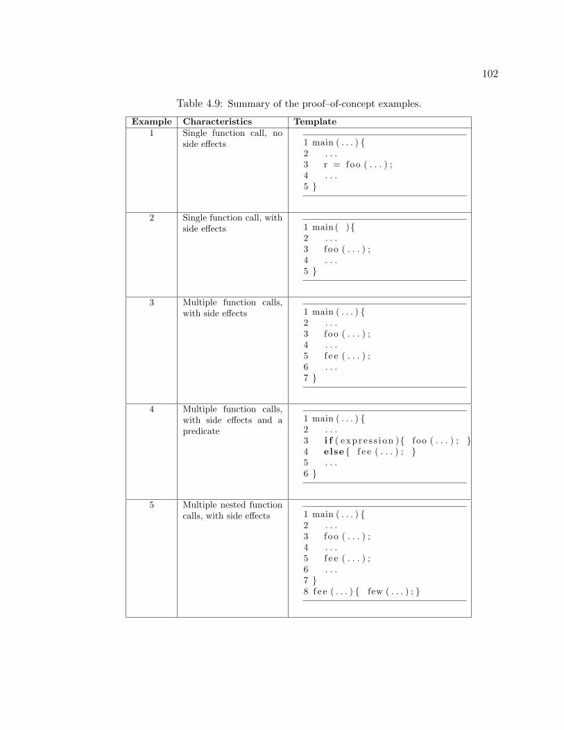
102

Table 4.9: Summary of the proof–of-concept examples.

Example Characteristics Template1 Single function call, no

side effects 1 main ( . . . ) {2 . . .3 r = foo ( . . . ) ;4 . . .5 }

2 Single function call, withside effects 1 main ( ){

2 . . .3 foo ( . . . ) ;4 . . .5 }

3 Multiple function calls,with side effects 1 main ( . . . ) {

2 . . .3 foo ( . . . ) ;4 . . .5 f e e ( . . . ) ;6 . . .7 }

4 Multiple function calls,with side effects and apredicate

1 main ( . . . ) {2 . . .3 i f ( exp r e s s i on ){ f oo ( . . . ) ; }4 else { f e e ( . . . ) ; }5 . . .6 }

5 Multiple nested functioncalls, with side effects 1 main ( . . . ) {

2 . . .3 foo ( . . . ) ;4 . . .5 f e e ( . . . ) ;6 . . .7 }8 f e e ( . . . ) { few ( . . . ) ; }

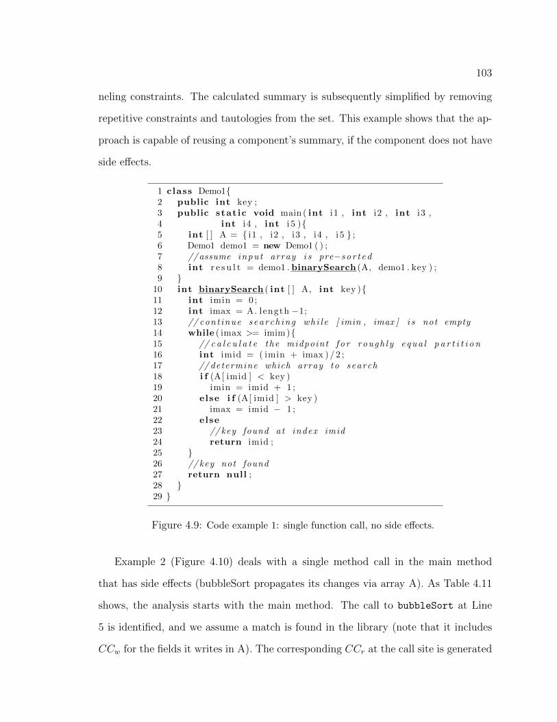
103

neling constraints. The calculated summary is subsequently simplified by removing

repetitive constraints and tautologies from the set. This example shows that the ap-

proach is capable of reusing a component’s summary, if the component does not have

side effects.

1 class Demo1{2 public int key ;3 public stat ic void main ( int i1 , int i2 , int i3 ,4 int i4 , int i 5 ){5 int [ ] A = { i1 , i2 , i3 , i4 , i 5 } ;6 Demo1 demo1 = new Demo1 ( ) ;7 //assume input array i s pre−so r t ed8 int r e s u l t = demo1 . binarySearch (A, demo1 . key ) ;9 }

10 int binarySearch ( int [ ] A, int key ){11 int imin = 0 ;12 int imax = A. length −1;13 // cont inue search ing wh i l e [ imin , imax ] i s not empty14 while ( imax >= imim ){15 // c a l c u l a t e the midpoint f o r rough ly equa l p a r t i t i o n16 int imid = ( imin + imax ) / 2 ;17 // determine which array to search18 i f (A[ imid ] < key )19 imin = imid + 1 ;20 else i f (A[ imid ] > key )21 imax = imid − 1 ;22 else23 // key found at index imid24 return imid ;25 }26 // key not found27 return null ;28 }29 }

Figure 4.9: Code example 1: single function call, no side effects.

Example 2 (Figure 4.10) deals with a single method call in the main method

that has side effects (bubbleSort propagates its changes via array A). As Table 4.11

shows, the analysis starts with the main method. The call to bubbleSort at Line

5 is identified, and we assume a match is found in the library (note that it includes

CCw for the fields it writes in A). The corresponding CCr at the call site is generated

104

Table 4.10: Constraint composition for code example 1.

Line # ComponentSummary

Description Constraints Source5-8 main target - computeUC

8 binarySearchCCr i1 == s1 ∧ i2 == s2 ∧

i3 == s3 ∧ i4 == s4 ∧i5 == s5 ∧ field.key ==s key

Custom-SE

size = 5 (ar-ray)+1(searchkey)

Summary6 s1 < s key ∧ s2 < s key ∧s3 < s key ∧ s4 > s key ∧s5 > s key

library

CCw result == null library

9 main Summary i1 == s1 ∧ i2 == s2 ∧i3 == s3 ∧ i4 == s4 ∧i5 == s5 ∧ field.key ==s key ∧ s1 < s key ∧ s2 <s key ∧ s3 < s key ∧ s4 >s key ∧ s5 > s key

computeUC

9 main Summary i1 < field.key ∧ i2 <field.key ∧ i3 <field.key ∧ i4 >field.key ∧ i5 > field.key

simplified

by calling Custom-SE. The analysis then traverses to the end of main at Line 6,

and calculates a summary for main by composing the summaries with channeling

constraints. The calculated summary is subsequently simplified. This example shows

that the approach can reuse a component’s summary, and can handle side effects

properly.

105

1 class Demo2{2 public stat ic void main ( int i1 , i2 , i3 , i4 , i 5 ){3 int [ ] A = { i1 , i2 , i3 , i4 , i 5 } ;4 Demo2 demo2 = new Demo1 ( ) ;5 demo2 . bubbleSort (A) ;6 }7 void bubbleSort ( int [ ] A){8 boolean swapped = true ;9 int temp ;

10 while ( swapped ){11 swapped = fa l se ;12 for ( int i =1; i <= A. length −1; i ++){13 i f (A[ i −1] > A[ i ] ) {14 //swap A[ i −1] and A[ i ]15 temp = A[ i −1] ;16 A[ i −1] = A[ i ] ;17 A[ i ] = temp ;18 swapped = true ;19 }20 }21 }22 }23 }

Figure 4.10: Code example 2: single function call, with side effects.

Example 3 (Figure 4.11) deals with two method calls in the main method. One of

them has side effects. As Table 4.12 shows, the analysis starts with the main method.

It first identifies the call to bubbleSort at Line 6, then the call to binarySearch at

Line 7. In this example, both callees have matching summaries that can be reused.

The analysis then traverses to the end of main at Line 7, and calculates a summary

for main by composing the summaries with channeling constraints. The calculated

summary is subsequently simplified. The final summary, in Line 6, captures a worst

case scenario for the program, because the bubbleSort method is used to sort an

array that is already sorted in reverse order, and the binarySearch method traverses

to the bottom of the search tree. This example shows that the approach is capable

of computing a worst case summary for a Java program by composing two worst case

summaries for its components together.

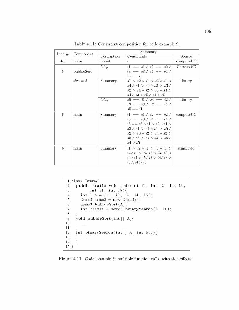
106




5 bubbleSortCCr i1 == s1 ∧ i2 == s2 ∧

i3 == s3 ∧ i4 == s4 ∧i5 == s5

Custom-SE

size = 5 Summary s1 > s2 ∧ s1 > s3 ∧ s1 >s4 ∧ s1 > s5 ∧ s2 > s3 ∧s2 > s4 ∧ s2 > s5 ∧ s3 >s4 ∧ s3 > s5 ∧ s4 > s5

library

CCw s5 == i1 ∧ s4 == i2 ∧s3 == i3 ∧ s2 == i4 ∧s5 == i1

library

6 main Summary i1 == s1 ∧ i2 == s2 ∧i3 == s3 ∧ i4 == s4 ∧i5 == s5 ∧ s1 > s2 ∧ s1 >s3 ∧ s1 > s4 ∧ s1 > s5 ∧s2 > s3 ∧ s2 > s4 ∧ s2 >s5 ∧ s3 > s4 ∧ s3 > s5 ∧s4 > s5

computeUC

6 main Summary i1 > i2 ∧ i1 > i3 ∧ i1 >i4∧i1 > i5∧i2 > i3∧i2 >i4∧i2 > i5∧i3 > i4∧i3 >i5 ∧ i4 > i5

simplified

1 class Demo3{2 public stat ic void main ( int i1 , int i2 , int i3 ,3 int i4 , int i 5 ){4 int [ ] A = { i1 , i2 , i3 , i4 , i 5 } ;5 Demo3 demo3 = new Demo3 ( ) ;6 demo3 . bubbleSort (A) ;7 int r e s u l t = demo3 . binarySearch (A, i 1 ) ;8 }9 void bubbleSort ( int [ ] A){

10 . . .11 }12 int binarySearch ( int [ ] A, int key ){13 . . .14 }15 }

Figure 4.11: Code example 3: multiple function calls, with side effects.

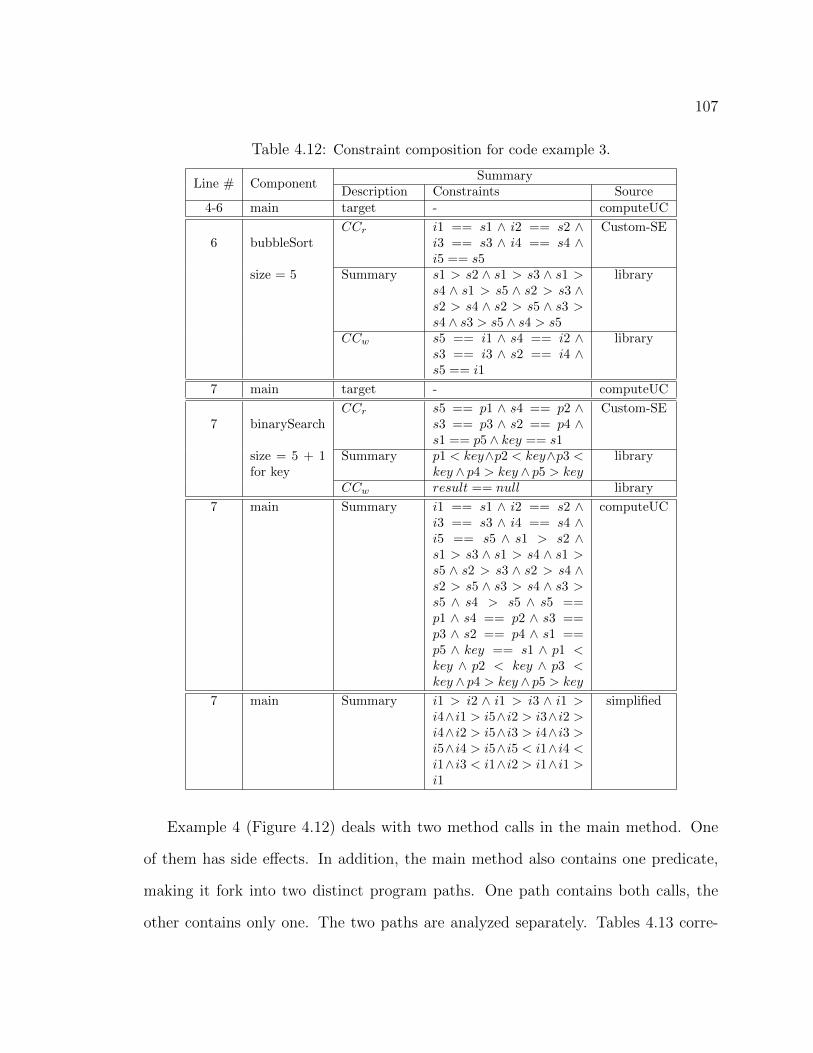
107





i3 == s3 ∧ i4 == s4 ∧i5 == s5

Custom-SE


library

CCw s5 == i1 ∧ s4 == i2 ∧s3 == i3 ∧ s2 == i4 ∧s5 == i1

library

7 main target - computeUC

7 binarySearchCCr s5 == p1 ∧ s4 == p2 ∧

s3 == p3 ∧ s2 == p4 ∧s1 == p5 ∧ key == s1

Custom-SE

size = 5 + 1for key

Summary p1 < key∧p2 < key∧p3 <key ∧ p4 > key ∧ p5 > key

library


7 main Summary i1 == s1 ∧ i2 == s2 ∧i3 == s3 ∧ i4 == s4 ∧i5 == s5 ∧ s1 > s2 ∧s1 > s3 ∧ s1 > s4 ∧ s1 >s5 ∧ s2 > s3 ∧ s2 > s4 ∧s2 > s5 ∧ s3 > s4 ∧ s3 >s5 ∧ s4 > s5 ∧ s5 ==p1 ∧ s4 == p2 ∧ s3 ==p3 ∧ s2 == p4 ∧ s1 ==p5 ∧ key == s1 ∧ p1 <key ∧ p2 < key ∧ p3 <key ∧ p4 > key ∧ p5 > key

computeUC

7 main Summary i1 > i2 ∧ i1 > i3 ∧ i1 >i4∧i1 > i5∧i2 > i3∧i2 >i4∧i2 > i5∧i3 > i4∧i3 >i5∧i4 > i5∧i5 < i1∧i4 <i1∧i3 < i1∧i2 > i1∧i1 >i1

simplified

Example 4 (Figure 4.12) deals with two method calls in the main method. One

of them has side effects. In addition, the main method also contains one predicate,

making it fork into two distinct program paths. One path contains both calls, the

other contains only one. The two paths are analyzed separately. Tables 4.13 corre-

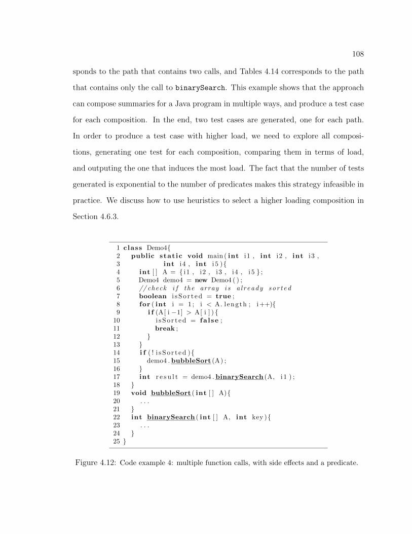
108

sponds to the path that contains two calls, and Tables 4.14 corresponds to the path

that contains only the call to binarySearch. This example shows that the approach

can compose summaries for a Java program in multiple ways, and produce a test case

for each composition. In the end, two test cases are generated, one for each path.

In order to produce a test case with higher load, we need to explore all composi-

tions, generating one test for each composition, comparing them in terms of load,

and outputing the one that induces the most load. The fact that the number of tests

generated is exponential to the number of predicates makes this strategy infeasible in

practice. We discuss how to use heuristics to select a higher loading composition in

Section 4.6.3.

1 class Demo4{2 public stat ic void main ( int i1 , int i2 , int i3 ,3 int i4 , int i 5 ){4 int [ ] A = { i1 , i2 , i3 , i4 , i 5 } ;5 Demo4 demo4 = new Demo4 ( ) ;6 // check i f the array i s a l r eady so r t ed7 boolean i s S o r t e d = true ;8 for ( int i = 1 ; i < A. length ; i ++){9 i f (A[ i −1] > A[ i ] ) {

10 i s S o r t e d = fa l se ;11 break ;12 }13 }14 i f ( ! i s S o r t e d ){15 demo4 . bubbleSort (A) ;16 }17 int r e s u l t = demo4 . binarySearch (A, i 1 ) ;18 }19 void bubbleSort ( int [ ] A){20 . . .21 }22 int binarySearch ( int [ ] A, int key ){23 . . .24 }25 }

Figure 4.12: Code example 4: multiple function calls, with side effects and a predicate.

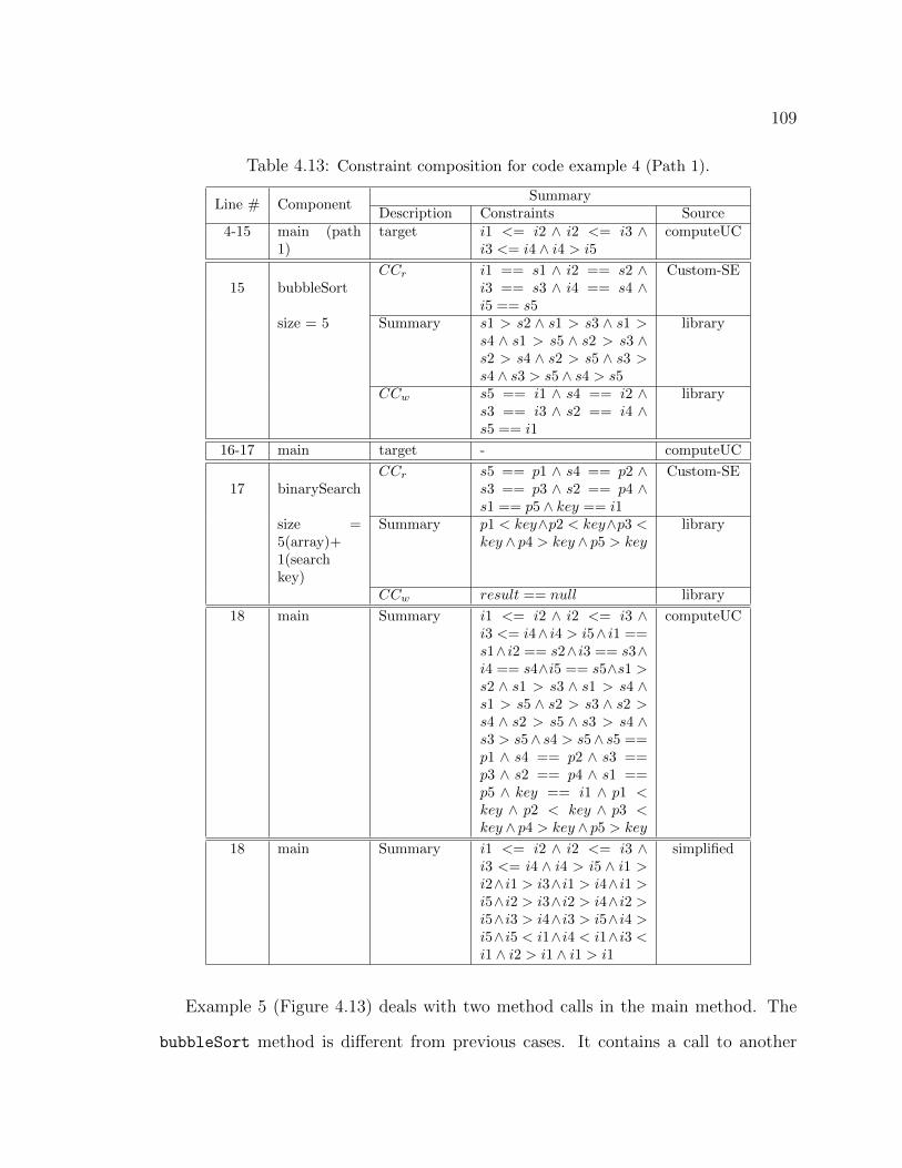
109

Table 4.13: Constraint composition for code example 4 (Path 1).


Description Constraints Source4-15 main (path

1)target i1 <= i2 ∧ i2 <= i3 ∧

i3 <= i4 ∧ i4 > i5computeUC


i3 == s3 ∧ i4 == s4 ∧i5 == s5

Custom-SE


library

CCw s5 == i1 ∧ s4 == i2 ∧s3 == i3 ∧ s2 == i4 ∧s5 == i1

library

16-17 main target - computeUC


s3 == p3 ∧ s2 == p4 ∧s1 == p5 ∧ key == i1

Custom-SE

size =5(array)+1(searchkey)


library


18 main Summary i1 <= i2 ∧ i2 <= i3 ∧i3 <= i4∧ i4 > i5∧ i1 ==s1∧ i2 == s2∧ i3 == s3∧i4 == s4∧i5 == s5∧s1 >s2 ∧ s1 > s3 ∧ s1 > s4 ∧s1 > s5 ∧ s2 > s3 ∧ s2 >s4 ∧ s2 > s5 ∧ s3 > s4 ∧s3 > s5∧ s4 > s5∧ s5 ==p1 ∧ s4 == p2 ∧ s3 ==p3 ∧ s2 == p4 ∧ s1 ==p5 ∧ key == i1 ∧ p1 <key ∧ p2 < key ∧ p3 <key ∧ p4 > key ∧ p5 > key

computeUC

18 main Summary i1 <= i2 ∧ i2 <= i3 ∧i3 <= i4 ∧ i4 > i5 ∧ i1 >i2∧i1 > i3∧i1 > i4∧i1 >i5∧i2 > i3∧i2 > i4∧i2 >i5∧i3 > i4∧i3 > i5∧i4 >i5∧i5 < i1∧i4 < i1∧i3 <i1 ∧ i2 > i1 ∧ i1 > i1

simplified

Example 5 (Figure 4.13) deals with two method calls in the main method. The

bubbleSort method is different from previous cases. It contains a call to another

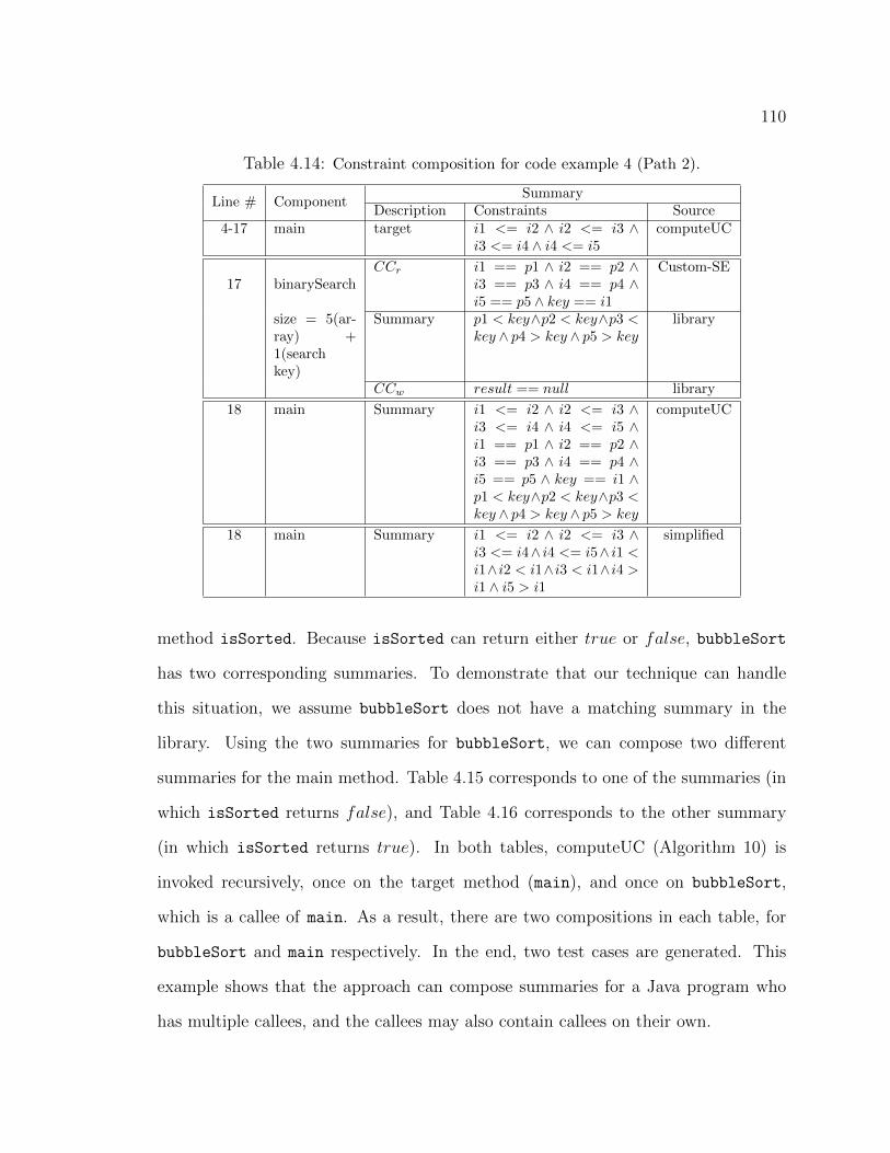
110



Description Constraints Source4-17 main target i1 <= i2 ∧ i2 <= i3 ∧

i3 <= i4 ∧ i4 <= i5computeUC

17 binarySearchCCr i1 == p1 ∧ i2 == p2 ∧

i3 == p3 ∧ i4 == p4 ∧i5 == p5 ∧ key == i1

Custom-SE

size = 5(ar-ray) +1(searchkey)


library


18 main Summary i1 <= i2 ∧ i2 <= i3 ∧i3 <= i4 ∧ i4 <= i5 ∧i1 == p1 ∧ i2 == p2 ∧i3 == p3 ∧ i4 == p4 ∧i5 == p5 ∧ key == i1 ∧p1 < key∧p2 < key∧p3 <key ∧ p4 > key ∧ p5 > key

computeUC

18 main Summary i1 <= i2 ∧ i2 <= i3 ∧i3 <= i4∧ i4 <= i5∧ i1 <i1∧i2 < i1∧i3 < i1∧i4 >i1 ∧ i5 > i1

simplified

method isSorted. Because isSorted can return either true or false, bubbleSort

has two corresponding summaries. To demonstrate that our technique can handle

this situation, we assume bubbleSort does not have a matching summary in the

library. Using the two summaries for bubbleSort, we can compose two different

summaries for the main method. Table 4.15 corresponds to one of the summaries (in

which isSorted returns false), and Table 4.16 corresponds to the other summary

(in which isSorted returns true). In both tables, computeUC (Algorithm 10) is

invoked recursively, once on the target method (main), and once on bubbleSort,

which is a callee of main. As a result, there are two compositions in each table, for

bubbleSort and main respectively. In the end, two test cases are generated. This

example shows that the approach can compose summaries for a Java program who

has multiple callees, and the callees may also contain callees on their own.

111

1 class Demo52 public stat ic void main ( int i1 , int i2 , int i3 ,3 int i4 , int i 5 ){4 int [ ] A = { s1 , s2 , s3 , s4 , s5 } ;5 Demo5 demo5 = new Demo5 ( ) ;6 demo5 . bubbleSort (A) ;7 int r e s u l t = binarySearch (A, i 1 ) ;8 }9 void bubbleSort ( int [ ] A){

10 i f ( ! i s S o r t e d (A)){11 boolean swapped = true ;12 int temp ;13 while ( swapped ){14 swapped = fa l se ;15 for ( int i =1; i <= A. length −1; i ++){16 i f (A[ i −1] > A[ i ] ) {17 //swap A[ i −1] and A[ i ]18 temp = A[ i −1] ;19 A[ i −1] = A[ i ] ;20 A[ i ] = temp ;21 swapped = true ;22 }23 }24 }25 }26 }27 boolean i s S o r t e d ( int [ ] A){28 for ( int i = 1 ; i < A. length ; i ++){29 i f (A[ i −1] > A[ i ] ) {30 return fa l se ;31 }32 }33 return true ;34 }35 int binarySearch ( int [ ] A, int key ){36 . . .37 }38 }

Figure 4.13: Code example 5: multiple nested function calls, with side effects.

112




10 bubbleSort(call site @6)

CCr i1 == s1 ∧ i2 == s2 ∧i3 == s3 ∧ i4 == s4 ∧i5 == s5

Custom-SE

10 isSortedCCr k1 == s1 ∧ k2 == s2 ∧

k3 == s3 ∧ k4 == s4 ∧k5 == s5

Custom-SE

size = 5 Summary k1 <= k2 ∧ k2 <= k3 ∧k3 <= k4 ∧ k4 > k5

library

CCw false library

10-26bubbleSort(call site @6)

Summary k1 == s1 ∧ k2 == s2 ∧k3 == s3 ∧ k4 == s4 ∧k5 == s5 ∧ k1 <= k2 ∧k2 <= k3 ∧ k3 <= k4 ∧k4 > k5 ∧ s1 > s2 ∧ s1 >s3 ∧ s1 > s4 ∧ s1 > s5 ∧s2 > s3 ∧ s2 > s4 ∧ s2 >s5 ∧ s3 > s4 ∧ s3 > s5 ∧s4 > s5

computeUC

CCw s1 == i5 ∧ s2 == i4 ∧s3 == i3 ∧ s4 == i2 ∧s5 == i1

Custom-SE



s3 == p3 ∧ s2 == p4 ∧s1 == p5 ∧ key == i1

Custom-SE

size = 5(ar-ray)+1(searchkey)


library


8 main Summary i1 <= i2 ∧ i2 <= i3 ∧i3 <= i4∧ i4 > i5∧ i1 ==s1∧ i2 == s2∧ i3 == s3∧i4 == s4∧i5 == s5∧s1 >s2 ∧ s1 > s3 ∧ s1 > s4 ∧s1 > s5 ∧ s2 > s3 ∧ s2 >s4 ∧ s2 > s5 ∧ s3 > s4 ∧s3 > s5∧ s4 > s5∧ s5 ==p1 ∧ s4 == p2 ∧ s3 ==p3 ∧ s2 == p4 ∧ s1 ==p5 ∧ key == i1 ∧ p1 <key ∧ p2 < key ∧ p3 <key ∧ p4 > key ∧ p5 > key

computeUC

8 main Summary i1 <= i2 ∧ i2 <= i3 ∧i3 <= i4 ∧ i4 > i5 ∧ i1 >i2∧i1 > i3∧i1 > i4∧i1 >i5∧i2 > i3∧i2 > i4∧i2 >i5∧i3 > i4∧i3 > i5∧i4 >i5∧i5 < i1∧i4 < i1∧i3 <i1 ∧ i2 > i1 ∧ i1 > i1

simplified

113




10 bubbleSort(call site @6)

CCr i1 == s1 ∧ i2 == s2 ∧i3 == s3 ∧ i4 == s4 ∧i5 == s5

Custom-SE

10 isSortedCCr k1 == s1 ∧ k2 == s2 ∧

k3 == s3 ∧ k4 == s4 ∧k5 == s5

Custom-SE

size = 5 Summary k1 <= k2 ∧ k2 <= k3 ∧k3 <= k4 ∧ k4 <= k5

library

CCw true library

10-26bubbleSort(call site @6)

Summary k1 == s1 ∧ k2 == s2 ∧k3 == s3 ∧ k4 == s4 ∧k5 == s5 ∧ k1 <= k2 ∧k2 <= k3 ∧ k3 <= k4 ∧k4 <= k5

computeUC

CCw s1 == i1 ∧ s2 == i2 ∧s3 == i3 ∧ s4 == i4 ∧s5 == i5

Custom-SE



s3 == p3 ∧ s4 == p4 ∧s5 == p5 ∧ key == i1

Custom-SE

size = 5(ar-ray)+1(searchkey)


library


8 main Summary i1 <= i2 ∧ i2 <= i3 ∧i3 <= i4 ∧ i4 <= i5 ∧i1 == s1 ∧ i2 == s2 ∧i3 == s3 ∧ i4 == s4 ∧i5 == s5 ∧ s1 == p1 ∧s2 == p2 ∧ s3 == p3 ∧s4 == p4 ∧ s5 == p5 ∧key == i1 ∧ p1 < key ∧p2 < key∧p3 < key∧p4 >key ∧ p5 > key

computeUC

8 main Summary i1 <= i2 ∧ i2 <= i3 ∧i3 <= i4∧ i4 <= i5∧ i1 <i1∧i2 < i1∧i3 < i1∧i4 >i1 ∧ i5 > i1

simplified

114

4.6.2 Richer Performance Summaries

The technique for handling pipelines needs only to consider the input / output sizes of

the summaries when doing summary matching. This is because the pipeline approach

works on a coarser granularity. Each component is a single program, and the number

of components in a pipeline is usually small (order of tens). For Java programs,

because each component is a single method, the approach works at a much finer

granularity level. Subtle incompatibilities between summaries can cause removal of

key constraints in the performance summaries, and the cumulative effect of such

unnecessary reduction may impact the induced load.

The performance degradation is more prominent, when the program under test

takes heap-allocated data structures, such as trees and linked lists, as inputs. A

modern symbolic execution engine (e.g., Symbolic PathFinder, the framework upon

which our technique is built) handles heap-allocated data via lazy initialization. SPF

starts execution of the method on inputs with uninitialized fields and it assign values

to these fields lazily, i.e., when they are first accessed during the methods symbolic

execution. As symbolic execution continues, each node of the execution tree denotes

a program state, which consists of the following information: 1) a program counter

that tracks the execution progress; 2) a set of constraints collected over symbolic

variables of primitive types; 3) the shape of the heap-allocated data structure on

which the program executes. Here the shape of the data structure is encoded as a set

of memory allocations and pointers. The shape information is essential to maintain

a precise symbolic execution of the target program.

However, when we use SLG to generate performance summaries, we only store

part of the program state: the set of constraints on primitive types. In addition we

also store tags on the size of inputs / outputs to assist matching. The size tags can

be viewed as naive abstractions of the shape information [4], which we omitted in this

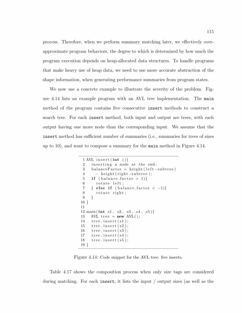
115

process. Therefore, when we perform summary matching later, we effectively over-

approximate program behaviors, the degree to which is determined by how much the

program execution depends on heap-allocated data structures. To handle programs

that make heavy use of heap data, we need to use more accurate abstraction of the

shape information, when generating performance summaries from program states.

We now use a concrete example to illustrate the severity of the problem. Fig-

ure 4.14 lists an example program with an AVL tree implementation. The main

method of the program contains five consecutive insert methods to construct a

search tree. For each insert method, both input and output are trees, with each

output having one more node than the corresponding input. We assume that the

insert method has sufficient number of summaries (i.e., summaries for trees of sizes

up to 10), and want to compose a summary for the main method in Figure 4.14.

1 AVL i n s e r t ( int i ){2 i n s e r t i n g a node at the end ;3 ba lanceFactor = he ight ( l e f t −subt ree )4 − he ight ( r ight−subt ree ) ;5 i f ( b a l a n c e f a c t o r > 1){6 r o t a t e l e f t ;7 } else i f ( b a l a n c e f a c t o r < −1){8 r o t a t e r i g h t ;9 }

10 }1112 main ( int s1 , s2 , s3 , s4 , s5 ){13 AVL t r e e = new AVL( ) ;14 t r e e . i n s e r t ( s1 ) ;15 t r e e . i n s e r t ( s2 ) ;16 t r e e . i n s e r t ( s3 ) ;17 t r e e . i n s e r t ( s4 ) ;18 t r e e . i n s e r t ( s5 ) ;19 }

Figure 4.14: Code snippet for the AVL tree: five inserts.

Table 4.17 shows the composition process when only size tags are considered

during matching. For each insert, it lists the input / output sizes (as well as the

116

Table 4.17: Handling AVL tree with five inserts (size match).

#Input Output

Constraintsshape size shape size

1st insert s1 1 s1 1 –

2nd insert s1 2

s1

s2 2 s1 < s2

3rd insert

s1

s2 3

s2

s1 s3 3 s1 < s2 ∧ s2 < s3

4th insert

s2

s1 s3 4

s2

s1 s3

s4 4 s1 < s2 ∧ s2 < s3 ∧ s3 < s4

5th insert

s2

s1 s3

s4 5

s2

s5 s3

s4 s1 5 s1 < s2 ∧ s2 < s3 ∧ s4 <s1 ∧ s5 < s1 ∧ s4 < s5

shape of the tree for comparison purpose), and the constraints collected by SLG. In

the table, each insert’s output size matches the next insert’s input size. Table 4.18

shows another scenario in the same format, when the shape of the tree is considered.

For example, in Table 4.18 the output tree of the 4th insert matches the input tree

of the 5th insert. While in Table 4.17, the output tree of the 4th insert does not

match the input tree of the 5th insert, although both of them having the same size

4.

Table 4.19 shows the evaluation on the test cases generated from the two scenarios.

As shown in the table, the scenario following shape match produces a test case that

induces 62% more load than the other scenario. This is because if the shape of the

tree is kept as new nodes are inserted, it is more likely to break the balance and force

rotation. This example clearly conveys the importance of more precise tags when

matching summaries.

117

Table 4.18: Handling AVL tree with five inserts (shape match).

#Input Output

Constraintsshape size shape size

1st insert s1 1 s1 1 –

2nd insert s1 2

s1

s2 2 s1 < s2

3rd insert

s1

s2 3

s2

s1 s3 3 s1 < s2 ∧ s2 < s3

4th insert

s2

s1 s3 4

s2

s1 s3

s4 4 s1 < s2 ∧ s2 < s3 ∧ s3 < s4

5th insert

s2

s1 s3

s4 5

s2

s1 s4

s5 s3 5 s1 < s2 ∧ s2 < s3 ∧ s3 <s4 ∧ s4 < s5

Table 4.19: Evaluation: AVL tree with five inserts.

Generated Test Load (bytecode count)Size matching scenario 385

Shape matching scenario 517

4.6.2.1 Revisiting the Approach to Generating Performance Summaries

We propose a slightly revised approach for generating performance summaries with

more precise metadata describing their properties, in order to enable a more precise

summary matching process that follows. First we present a few definitions.

Definition 4.6.2 Shape Metadata: A set of metadata encoding the shape of the heap-

allocated data structure in terms of objects created by memory allocations, and the

reference pointers among the objects.

For example, metadata for a tree data structure (as in the AVL tree example)

could include node objects and the children reference within each node. Note that

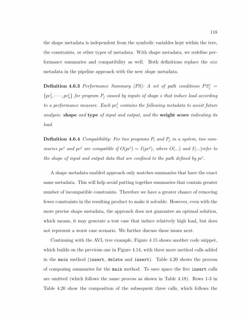
118

the shape metadata is independent from the symbolic variables kept within the tree,

the constraints, or other types of metadata. With shape metadata, we redefine per-

formance summaries and compatibility as well. Both definitions replace the size

metadata in the pipeline approach with the new shape metadata.

Definition 4.6.3 Performance Summary (PS): A set of path conditions PSsj =

{pcj1, · · · , pcjn} for program Pj caused by inputs of shape s that induce load according

to a performance measure. Each pcji contains the following metadata to assist future

analysis: shape and type of input and output, and the weight score indicating its

load.

Definition 4.6.4 Compatibility: For two programs Pi and Pj in a system, two sum-

maries pci and pcj are compatible if O(pci) = I(pcj), where O(...) and I(...)refer to

the shape of input and output data that are confined to the path defined by pci.

A shape metadata enabled approach only matches summaries that have the exact

same metadata. This will help avoid putting together summaries that contain greater

number of incompatible constraints. Therefore we have a greater chance of removing

fewer constraints in the resulting product to make it solvable. However, even with the

more precise shape metadata, the approach does not guarantee an optimal solution,

which means, it may generate a test case that induce relatively high load, but does

not represent a worst case scenario. We further discuss these issues next.

Continuing with the AVL tree example, Figure 4.15 shows another code snippet,

which builds on the previous one in Figure 4.14, with three more method calls added

in the main method (insert, delete and insert). Table 4.20 shows the process

of composing summaries for the main method. To save space the five insert calls

are omitted (which follows the same process as shown in Table 4.18). Rows 1-3 in

Table 4.20 show the composition of the subsequent three calls, which follows the

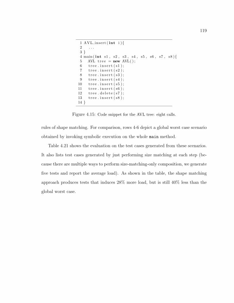
119

1 AVL insert ( int i ){2 . . .3 }4 main ( int s1 , s2 , s3 , s4 , s5 , s6 , s7 , s8 ){5 AVL t r e e = new AVL( ) ;6 t r e e . i n s e r t ( s1 ) ;7 t r e e . i n s e r t ( s2 ) ;8 t r e e . i n s e r t ( s3 ) ;9 t r e e . i n s e r t ( s4 ) ;

10 t r e e . i n s e r t ( s5 ) ;11 t r e e . i n s e r t ( s6 ) ;12 t r e e . d e l e t e ( s7 ) ;13 t r e e . i n s e r t ( s8 ) ;14 }

Figure 4.15: Code snippet for the AVL tree: eight calls.

rules of shape matching. For comparison, rows 4-6 depict a global worst case scenario

obtained by invoking symbolic execution on the whole main method.

Table 4.21 shows the evaluation on the test cases generated from these scenarios.

It also lists test cases generated by just performing size matching at each step (be-

cause there are multiple ways to perform size-matching-only composition, we generate

five tests and report the average load). As shown in the table, the shape matching

approach produces tests that induces 28% more load, but is still 40% less than the

global worst case.

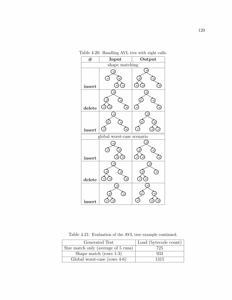
120

Table 4.20: Handling AVL tree with eight calls.

# Input Outputshape matching

insert

s2

s1 s4

s5 s3

s4

s5 s2

s3 s1 s6

delete

s4

s5 s2

s3 s1 s6

s3

s5 s2

s1 s6

insert

s3

s5 s2

s1 s6

s3

s6 s2

s1 s7 s5

global worst-case scenario

insert

s2

s1 s4

s5 s3

s4

s5 s2

s3 s1 s6

delete

s4

s5 s2

s3 s1 s6

s4

s5 s2

s3 s1

insert

s4

s5 s2

s3 s1

s2

s4 s1

s7 s5 s3

Table 4.21: Evaluation of the AVL tree example continued.

Generated Test Load (bytecode count)Size match only (average of 5 runs) 725

Shape match (rows 1-3) 933Global worst-case (rows 4-6) 1315

121

4.6.3 A New Strategy for Summary Composition

The complex nature of Java programs makes the technique for selecting summaries

for composition not suitable anymore. We will use a concrete example to illustrate

the new challenges. Consider the code snippet in Figure 4.12. The predicate at

Line 15 forks the execution into two paths, one containing both calls to bubbleSort

and binarySearch, the other only contains binarySearch. The path that contains

both calls induces more load, and should be chosen for test generation. One way to

identify the more expensive path is to explore both paths. However, the number of

paths grows exponentially with respect to the number of predicates. For example, on

a program with 4 predicates, the approach may need to traverse 16 paths to identify

the most expensive one. On the other extreme, an alternative approach that we have

used previously in handling pipelines is to use a greedy forward matching strategy.

However, this strategy does not always work for that type of examples, and in general

for programs with many paths where the first path may not be the one that induces

the most load. A greedy approach would first select a most expensive summary for

Lines 9-13. But this early choice will lead to the path that only contains the call

to binarySearch and skip bubbleSort at Line 15, making it a poor choice for load

testing.

4.6.3.1 Revisiting the Approach to Composition

Instead of using either exhaustive or greedy strategies, we conjecture that alternative

approaches, such as a heuristic search strategy, can be used to solve this problem,

hoping that a search strategy would strike a balance between the two extremes. Con-

ceptually, the proposed search strategy works on the component level, in which the

static call graph of the program forms the search space of potential compositions.

The goal of the search process is to find one composition that corresponds to the

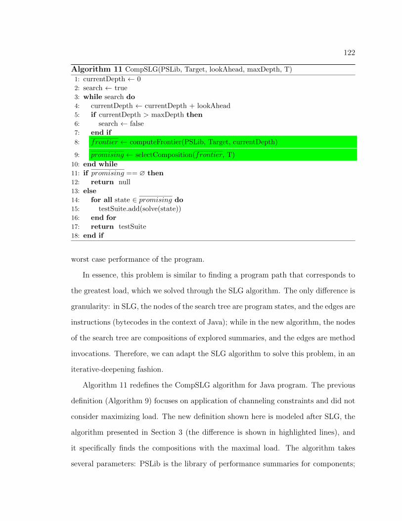
122

Algorithm 11 CompSLG(PSLib, Target, lookAhead, maxDepth, T)

1: currentDepth ← 02: search ← true3: while search do4: currentDepth ← currentDepth + lookAhead5: if currentDepth > maxDepth then6: search ← false7: end if

8: frontier ← computeFrontier(PSLib, Target, currentDepth)

9: promising ← selectComposition(frontier, T)

10: end while11: if promising == ∅ then12: return null13: else14: for all state ∈ promising do15: testSuite.add(solve(state))16: end for17: return testSuite18: end if

worst case performance of the program.

In essence, this problem is similar to finding a program path that corresponds to

the greatest load, which we solved through the SLG algorithm. The only difference is

granularity: in SLG, the nodes of the search tree are program states, and the edges are

instructions (bytecodes in the context of Java); while in the new algorithm, the nodes

of the search tree are compositions of explored summaries, and the edges are method

invocations. Therefore, we can adapt the SLG algorithm to solve this problem, in an

iterative-deepening fashion.

Algorithm 11 redefines the CompSLG algorithm for Java program. The previous

definition (Algorithm 9) focuses on application of channeling constraints and did not

consider maximizing load. The new definition shown here is modeled after SLG, the

algorithm presented in Section 3 (the difference is shown in highlighted lines), and

it specifically finds the compositions with the maximal load. The algorithm takes

several parameters: PSLib is the library of performance summaries for components;

123

Target is the target method against which a load test is generated; and T is the

number of tests to be generated; lookAhead and maxDepth are used in the same way

as in SLG.

Algorithm 11 invokes a few helper functions. Function computeFrontier traverses

all possible paths that originate from the target method and up to the designated

depth. It returns one constraint set (UC) for each such path. It can be implemented

by modifying computeUC (Algorithm 10), with two extensions: 1) computeUC only

traverses one path at a time. At Line 2 of Algorithm 10, the lookup function returns

only one matching summary. We can update this function to return all matching

summaries, allowing computeUC to explore each one (use a queue to hold intermediate

results), and return all explored paths; 2) computeUC does not stop at a specified

depth. We can use a counter to track recursion depth and stop when exceeding the

designated depth.

Function selectComposition selects promising paths at each frontier to continue,

and prune the others. It uses heuristics to choose a promising path, in terms of its

potential to induce load. We can reuse the available heuristics in SLG, such as

selecting the paths with the most accumulated weight score, or we can devise new

heuristics by taking advantage of the metadata associated with the components. For

example, if one component has a summary whose weight dominates the summaries of

other components, we can devise a heuristic that always selects the component with

the dominating summary. Alternatively, if there are several summaries of comparable

weight, we can devise a heuristic that selects distinct summary for each composition.

This last heuristic not only steers towards higher load, but also promotes diversity

among generated tests.

Algorithm 11 works as follows. As long as the current search depth is less than

maxDepth, It iterates on the following steps. First it attempts to explore all possible

124

paths up to lookAhead depth (Line 8). Then it uses heuristics to select promising

paths to continue on the next iteration (Line 9). When iteration stops, it solves

constraints associated to each remaining promising path, and reruns the test suite

(Line 14-17). The savings are achieved through pruning of the paths that are not

selected to continue.

Revisiting the example. Next we revisit the code snippet in Figure 4.12, applying

the new CompSLG algorithm on it. As shown before, this program has two paths.

one calls binarySearch, the other calls both bubbleSort and binarySearch. If we

set lookAhead to 1, after the first iteration, we would have explored two paths: Path

1: up to the call to bubbleSort; and Path 2: up to the call to binarySearch. The

algorithm then selects Path 1 to continue, because bubbleSort induces more load

than binarySearch. On the second iteration it finishes on Path 1 and generates a

load test. Note that this example does not explore full potential of the algorithm,

because the paths in the example are too short. Clearly for more complex programs

with more paths, lookAhead would have to be tweaked as well as the other parameters

of Algorithm 11 to favor the paths that are best aligned with the interest of the user.

4.7 Summary

This chapter presents a compositional approach, CompSLG, which can automatically

generate load tests for complex programs. CompSLG uses emerging symbolic exe-

cution based techniques to analyze the performance of each system component in

isolation, summarize the results of those analyses, and then perform a global analy-

sis across those summaries to generate load tests for the whole system. CompSLG

achieves gains in both efficiency and scalability by avoiding a search on the whole pro-

gram path space, and by reusing previously computed summaries to save on repetitive

125

computations.

In its current form, CompSLG is fully automated to handle any system that is

structured in the form of a software pipeline (such as a Unix pipeline or an XML

pipeline). A study of CompSLG revealed that it can generate load tests for pipelines

where SLG alone would not scale up, and it is much more cost effective than either

SLG applied to single components or Random test generation.

We also investigated how to extend CompSLG to enable its application to Java

programs, in which each method considered is a component. The extension includes

a new approach to generating channeling constraints, generating performance sum-

maries with more precise metadata, and an adapted strategy for composing sum-

maries. Although the extended version is not yet fully implemented, we showed the

viability of the approach with several proof-of-concept examples.

126

Chapter 5

Amplifying Tests to Validate

Exception Handling Code

As part of non-functional requirements, external resources impose contextual con-

straints on software systems that must interact with them. One way to improve

robustness of software is to use exception handling constructs. However, a faulty

implementation of exception handling code may introduce bugs that undermine the

overall quality of the software. In this chapter we present a white box exhaustive tech-

nique for detecting faulty implementations of exception handling constructs. The

technique is white box in a sense that it first instruments the target program by

adding a mocking device to take the place of the external resources of interest. It

then exhaustively amplifies the space of exceptional program behavior explored by

each test and associated with an external resource up to a user-defined number of

invocations.1

We first study the magnitude of the problem in Section 5.1. In Section 5.2 we

1Portions of the material presented in this chapter have appeared in a paper by Zhang et al.[136]. The material presented in this chapter provides an extended study of the technique. We willrefer to the original study presented in [136] as Phase 1, and the extended study as Phase 2.

127

present a motivating example showing the difficulties in exposing faulty exceptional

behavior and how we propose to solve it. Section 5.3 details the design and imple-

mentation of the technique. Section 5.4 presents a two-phase extensive study of the

technique.

5.1 Magnitude of the Problem

In this section we study the prevalence of faults associated with code that handles

exceptions. The study focuses on free popular applications for the Android plat-

form which rely extensively on APIs that work with external resources like wireless

connections, databases, GPS, or bluetooth.

The selection of artifacts for the study was conducted in two phases. Phase 1

consisted of our preliminary assessment of the approach [136]. Phase 2 corresponds

to this extended effort for providing a more thorough study of the approach, which

includes three new artifacts and a more extensive analysis. For the five applications

that were included in Phase 1, the selection process consisted of the following steps.

First, we collected a pool of 210 candidate applications from the following sources:

Wikipedia [125] (121), Le Wiki Koumbit [77] (40), Trac [121] (15), OpenStreetMap-

Wiki [87] (8), and Android Open Source DB [7] (26). We then use statistics provided

by Cyrket [31] to identify the applications with more than 50K downloads. This left

us with 25 applications. Because we are interested in applications with certain level

of development maturity, we refined our selection criteria by retaining applications

that 1) had an active and public bug tracking repository (excluded 15 apps), 2) had

multiple versions (excluded none), and 3) shipped with a unit test suite (excluded 5

more). These constraints left us with 5 applications: myTracks [84], a geo-tagging

application; XBMC remote [126], a remote control for the XBMC media center; Bar-

128

Table 5.1: Summary of artifacts.

Phase Application Resource API Version LOCUnit Test Suite# Execution

Time (sec)

1

Barcode Scanner android.net r1220 18170 117 275Keepassdroid android.database /

android.netv0.9.3 7713 34 102

myTracks android.database /android.location

r195 5918 55 367

SipDroidVoIP android.net r340 18150 39 135XBMC remote android.net / an-

droid.bluetoothr317 10880 78 234

2Android Wifi Tether android.net r170 18828 76 214K-9 Mail android.net / an-

droid.databaser512 34880 215 748

Open GPS Tracker android.location /android.database

r195 14156 85 308

code Scanner 2, a retriever of online information; Keepassdroid [71], a password keeper

that syncs with cloud services; and SipDroidVoIP [111], a voice over IP client. All

data in Phase 1 was collected between April and August 2011.

In Phase 2, we add three more applications following the same selection process,

but use Android market statistics provided by another source called AndroLib [9],

because Cyrket has not been accessible since 2012. In addition we excluded the

applications that were already selected in Phase 1. In the end we added three new

applications: Open GPS Tracker [86], a fitness application with GPS tagging function;

K-9 Mail [70], an email client; and Android Wifi Tether [8], an utility application

that provides wifi signal broadcasting capability. All data in Phase 2 was collected

between September and November 2012.

Table 5.1 provides a summary of the artifacts. The first five applications are from

Phase 1, and the other three correspond to Phase 2. Column “Resource API” shows

the types of resource APIs the application calls. Because many external resources are

managed through APIs, we decided to focus on the ones that use the Android API to

2The repository link for this app has not been accessible at the time of dissertation defense.

129

Table 5.2: Classification of confirmed and fixed bug reports.

ApplicationBug reports - Confirmed and Fixed

Total Keywords Exceptions Exceptions withScreening External Resources

Barcode Scanner 136 72 47 17 (13%)Keepassdroid 45 29 23 16 (36%)myTracks 46 28 21 11 (24%)SipDroidVoIP 252 107 39 27 (11%)XBMC remote 105 51 39 27 (26%)

Android Wifi Tether 54 32 26 14 (26%)K-9 Mail 687 289 99 39 (6%)Open GPS Tracker 100 34 21 14 (14%)

Total 1425 642 315 165 (12%)Average 178 80 39 21 (12%)

manage communication and sensing, because of their high rate of invocations by the

selected applications. The version of each application that we use for the evaluation

of the technique presented later in the thesis corresponds to the oldest version against

which a bug report is available. Columns “Version” and “LOC” denote the chosen

version and lines of code respectively. Column “Unit Test Suite” denotes the number

of unit tests shipped with each application, and the time it takes to run the available

test suites in the Android emulator [6].

The repositories held more than eight thousand bug reports. Among those, 1,425

were confirmed by the developers and addressed through a code revision. Utilizing the

bug repositories’ search facilities we then identified the bug reports that mentioned

the keywords exception, throw, or catch, which resulted in 642 reports. We then

examined each of those bug reports to identify the ones that were caused at least

in part by incomplete or erroneous coding of exception handlers. We found that

315 of the confirmed and fixed bug reports resulted in either adding new exception

handlers, modifying existing handlers, or refactoring handlers in various places. Last,

we analyzed each report in further detail to identify the ones that had to do with

exceptions thrown when services associated with the localization, bluetooth, database,

130

or network resources were invoked. These are the four types of resources that we

deemed interesting because of their noisy, diverse, and unpredictable nature.

Our detailed findings are reported in Table 5.2. Column “Total” shows the total

number of reports that were confirmed and linked to a fix. Column “Keywords

Screening” corresponds to our initial screening of the reports based on keywords

exception, throw, or catch. Columns “Exception” and “Exceptions with External

Resources” report the counts of the more detailed analyses. Even for the small set of

four external resources we examined, the data suggests that 22% of the confirmed and

fixed bugs have to do with poor exceptional handling code, and that 12% correspond

to interactions with external resources.

These findings must be taken in light of the scope of the study. We study eight

applications in a domain where we suspected troubles with exception handling because

of the types of resources being managed. Still, there are literally tens of thousands

of applications like this deployed and we expect for these findings to generalize to

them. We also echo the threat to validity often raised when dealing with such open

source repositories in terms of their noise, which is compounded by the fact that the

analysis of the bug reports required some level of judgement by one of the authors

and as such is subject to experimentation bias.

Even in light of these limitations, these findings support what we had informally

observed in terms of the magnitude of the problem associated with exceptional behav-

ior caused by external resources. With these issues in mind, we proceed to illustrate

what makes exposing these faults difficult and how the proposed approach addresses

those challenges.

131

5.2 Difficulties in Exposing Faulty Exceptional Be-

havior

Figure 5.1 shows a code excerpt from the Android application XBMC Remote which

implements a remote control for the XBMC media player and multimedia center

application. Lines 1-5 correspond to a test case driver we incorporated to simplified

the setup for presentation. The driver sets an http connection and then attempts to

retrieve content from the XBMC media server. It first invokes the method Connection

at Line 6, which subsequently calls two methods (Lines 12 and 16), setResponseFormat

attempts to format an http request for subsequent data fetching, and getSystem-

Info fetches basic system information of the server. If the connection is successful,

the networkManager.netStatus flag is set to true. After a successful connection, the

method getCurrentlyPlaying at Line 20 is then called to fetch a list of currently

playing music and videos.

All three methods at Lines 12, 16 and 20 use a subroutine query (Lines 28-39) to

communicate with the server application. The query method attempts to establish

an URL connection and fetch contents. The API call at line 31 can throw an IO-

Exception if the connection is down. This exception is caught by the catch clause

(Line 35), which calls mErrorHandler.handle, a centralized error handler (Lines 41-

54). When the catch clause for IOException (line 47) is executed, an attempt to

renew the connection is performed.

A bug report issued against this code and deemed high priority by the developers,

indicated that the application crashed at launch when the web connection became

intermittent3. The report’s trace log shows that the crash was caused by an elaborated

series of successful and failed queries to the API managing the connection. For the

3http://code.google.com/p/android-xbmcremote/issues/detail?id=84

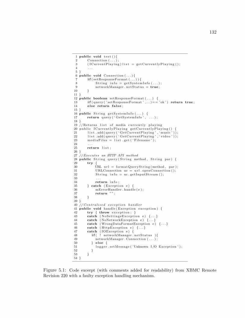
132

1 public void t e s t ( ){2 Connection ( . . . ) ;3 ( ICurrentPlay ing ) l i s t = getCurrent lyPlay ing ( ) ;4 . . .5 }6 public void Connection ( . . . ) {7 i f ( setResponseFormat ( . . . ) ) {8 St r ing i n f o = getSystemInfo ( . . . ) ;9 networkManager . netStatus = true ;

10 }11 }12 public boolean setResponseFormat ( . . . ) {13 i f ( query ( ’ setResponseFormat ’ , . . . )== ’ ok ’ ) return true ;14 else return fa l se ;15 }16 public St r ing getSystemInfo ( . . . ) {17 return query ( ‘ GetSystemInfo ’ , . . . ) ;18 }19 //Returns l i s t o f media cu r r en t l y p lay ing20 pub l i c ICurrent lyP lay ing getCurrent lyPlay ing ( ) {21 l i s t . add ( query ( ‘ GetCurrentPlaying ’ , ‘ music ’ ) ) ;22 l i s t . add ( query ( ‘ GetCurrentPlaying ’ , ‘ v ideo ’ ) ) ;23 mediaFi l e s = l i s t . get ( ‘ Filename ’ ) ;24 . . .25 return l i s t ;26 }27 //Executes an HTTP API method28 public St r ing query ( S t r ing method , S t r ing par ) {29 try {30 URL ur l = formatQueryStr ing (method , par ) ;31 URLConnection uc = ur l . openConnection ( ) ;32 St r ing i n f o = uc . getInputStream ( ) ;33 . . .34 return i n f o ;35 } catch ( Exception e ) {36 mErrorHandler . handle ( e ) ;37 return ”” ;38 }39 }40 // Cen t ra l i z ed excep t ion handler41 public void handle ( Exception except ion ) {42 try { throw except ion ; }43 catch ( NoSett ingsExcept ion e ) { . . . }44 catch ( NoNetworkException e ) { . . . }45 catch (WrongDataFormatException e ) { . . . }46 catch ( HttpException e ) { . . . }47 catch ( IOException e ) {48 i f ( ! networkManager . netStatus ){49 networkManager . Connection ( . . . ) ;50 } else {51 l ogg e r . setMessage ( ’Unknown I /O Exception ’ ) ;52 }53 }54 }

Figure 5.1: Code excerpt (with comments added for readability) from XBMC RemoteRevision 220 with a faulty exception handling mechanism.

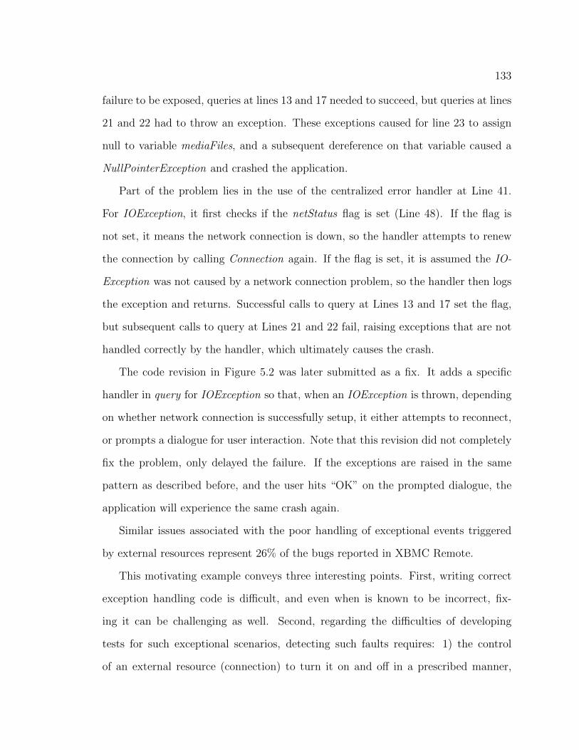
133

failure to be exposed, queries at lines 13 and 17 needed to succeed, but queries at lines

21 and 22 had to throw an exception. These exceptions caused for line 23 to assign

null to variable mediaFiles, and a subsequent dereference on that variable caused a

NullPointerException and crashed the application.

Part of the problem lies in the use of the centralized error handler at Line 41.

For IOException, it first checks if the netStatus flag is set (Line 48). If the flag is

not set, it means the network connection is down, so the handler attempts to renew

the connection by calling Connection again. If the flag is set, it is assumed the IO-

Exception was not caused by a network connection problem, so the handler then logs

the exception and returns. Successful calls to query at Lines 13 and 17 set the flag,

but subsequent calls to query at Lines 21 and 22 fail, raising exceptions that are not

handled correctly by the handler, which ultimately causes the crash.

The code revision in Figure 5.2 was later submitted as a fix. It adds a specific

handler in query for IOException so that, when an IOException is thrown, depending

on whether network connection is successfully setup, it either attempts to reconnect,

or prompts a dialogue for user interaction. Note that this revision did not completely

fix the problem, only delayed the failure. If the exceptions are raised in the same

pattern as described before, and the user hits “OK” on the prompted dialogue, the

application will experience the same crash again.

Similar issues associated with the poor handling of exceptional events triggered

by external resources represent 26% of the bugs reported in XBMC Remote.

This motivating example conveys three interesting points. First, writing correct

exception handling code is difficult, and even when is known to be incorrect, fix-

ing it can be challenging as well. Second, regarding the difficulties of developing

tests for such exceptional scenarios, detecting such faults requires: 1) the control

of an external resource (connection) to turn it on and off in a prescribed manner,

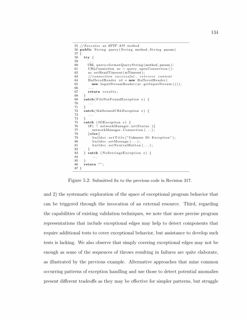
134

55 //Executes an HTTP API method56 public St r ing query ( S t r ing method , S t r ing param)57 {58 try {59 . . .60 URL query=formatQueryStr ing (method , param ) ;61 URLConnection uc = query . openConnection ( ) ;62 uc . setReadTimeout (mTimeout ) ;63 // connect ion suc c e s s f u l , r e t r i e v e content64 BufferedReader rd = new BufferedReader (65 new InputStreamReader ( uc . getInputStream ( ) ) ) ;66 . . .67 return r e s u l t s ;68 }69 catch ( FileNotFoundException e ) {70 . . .71 }72 catch (MalformedURLException e ) {73 . . .74 }75 catch ( IOException e ) {76 i f ( ! networkManager . netStatus ){77 networkManager . Connection ( . . . ) ;78 } else {79 bu i l d e r . s e tT i t l e ( ”Unknown IO Exception ” ) ;80 bu i l d e r . setMessage ( . . . ) ;81 bu i l d e r . setNeutra lButton ( . . . ) ;82 }83 } catch ( NoSett ingsExcept ion e ) {84 . . .85 }86 return ”” ;87 }

Figure 5.2: Submitted fix to the previous code in Revision 317.

and 2) the systematic exploration of the space of exceptional program behavior that

can be triggered through the invocation of an external resource. Third, regarding

the capabilities of existing validation techniques, we note that more precise program

representations that include exceptional edges may help to detect components that

require additional tests to cover exceptional behavior, but assistance to develop such

tests is lacking. We also observe that simply covering exceptional edges may not be

enough as some of the sequences of throws resulting in failures are quite elaborate,

as illustrated by the previous example. Alternative approaches that mine common

occurring patterns of exception handling and use those to detect potential anomalies

present different tradeoffs as they may be effective for simpler patterns, but struggle

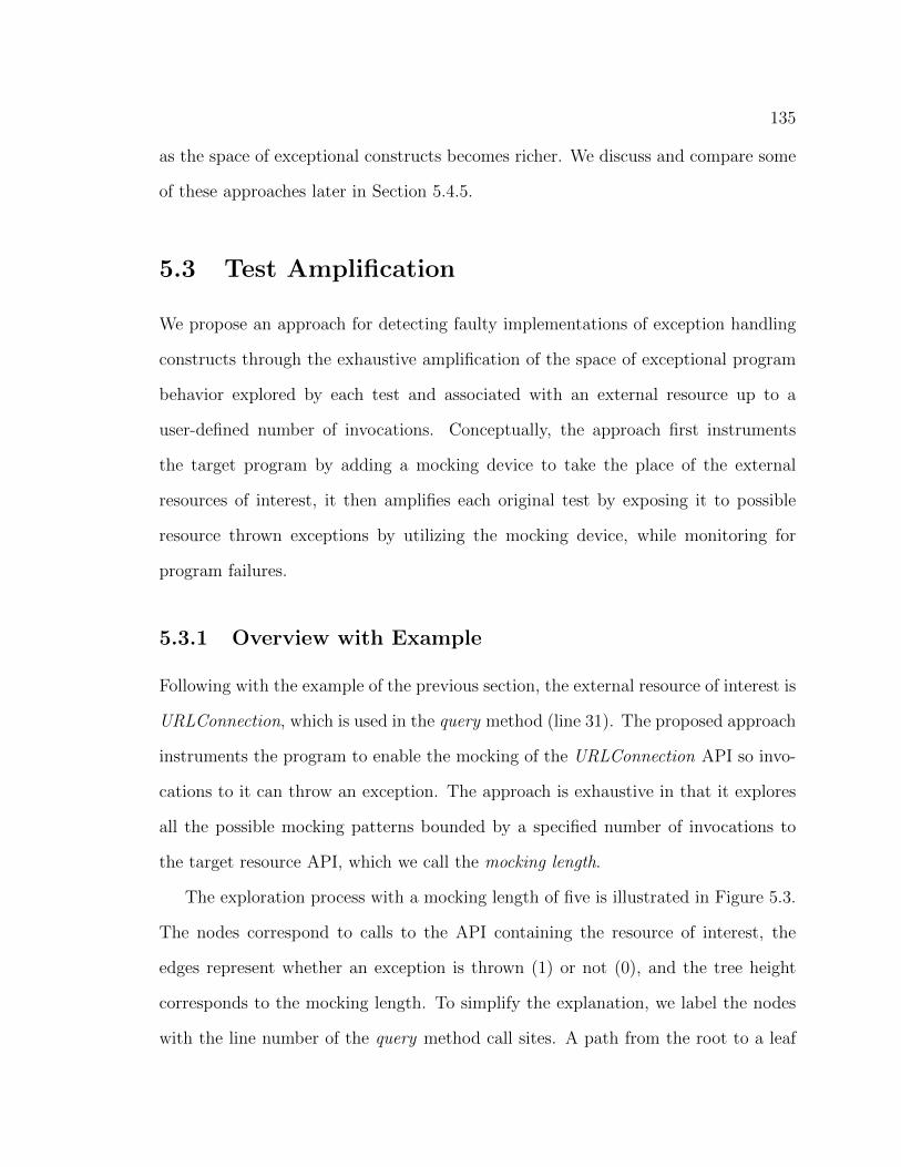
135

as the space of exceptional constructs becomes richer. We discuss and compare some

of these approaches later in Section 5.4.5.

5.3 Test Amplification

We propose an approach for detecting faulty implementations of exception handling

constructs through the exhaustive amplification of the space of exceptional program

behavior explored by each test and associated with an external resource up to a

user-defined number of invocations. Conceptually, the approach first instruments

the target program by adding a mocking device to take the place of the external

resources of interest, it then amplifies each original test by exposing it to possible

resource thrown exceptions by utilizing the mocking device, while monitoring for

program failures.

5.3.1 Overview with Example

Following with the example of the previous section, the external resource of interest is

URLConnection, which is used in the query method (line 31). The proposed approach

instruments the program to enable the mocking of the URLConnection API so invo-

cations to it can throw an exception. The approach is exhaustive in that it explores

all the possible mocking patterns bounded by a specified number of invocations to

the target resource API, which we call the mocking length.

The exploration process with a mocking length of five is illustrated in Figure 5.3.

The nodes correspond to calls to the API containing the resource of interest, the

edges represent whether an exception is thrown (1) or not (0), and the tree height

corresponds to the mocking length. To simplify the explanation, we label the nodes

with the line number of the query method call sites. A path from the root to a leaf

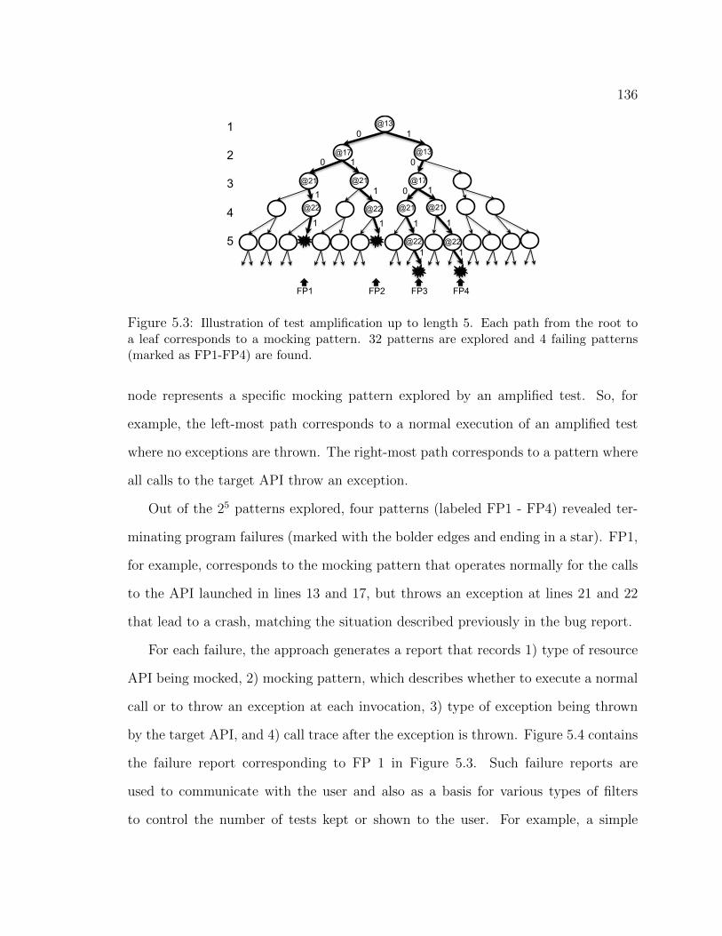
136

1 2 3 4 5

0

1

1

0 0

0

1

111

1 1 1 1

1

@13

@17

@21

@22

@21

@22

@13

@17

@21 @21

@22 @22

FP1 FP2 FP3 FP4

Figure 5.3: Illustration of test amplification up to length 5. Each path from the root toa leaf corresponds to a mocking pattern. 32 patterns are explored and 4 failing patterns(marked as FP1-FP4) are found.

node represents a specific mocking pattern explored by an amplified test. So, for

example, the left-most path corresponds to a normal execution of an amplified test

where no exceptions are thrown. The right-most path corresponds to a pattern where

all calls to the target API throw an exception.

Out of the 25 patterns explored, four patterns (labeled FP1 - FP4) revealed ter-

minating program failures (marked with the bolder edges and ending in a star). FP1,

for example, corresponds to the mocking pattern that operates normally for the calls

to the API launched in lines 13 and 17, but throws an exception at lines 21 and 22

that lead to a crash, matching the situation described previously in the bug report.

For each failure, the approach generates a report that records 1) type of resource

API being mocked, 2) mocking pattern, which describes whether to execute a normal

call or to throw an exception at each invocation, 3) type of exception being thrown

by the target API, and 4) call trace after the exception is thrown. Figure 5.4 contains

the failure report corresponding to FP 1 in Figure 5.3. Such failure reports are

used to communicate with the user and also as a basis for various types of filters

to control the number of tests kept or shown to the user. For example, a simple

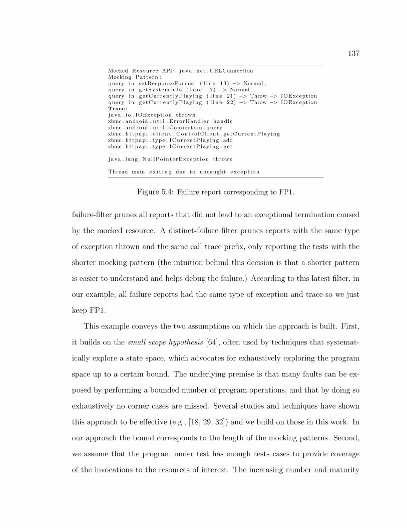
137

Mocked Resource API : java . net . URLConnectionMocking Pattern :query in setResponseFormat ( l i n e 13) −> Normal ,query in getSystemInfo ( l i n e 17) −> Normal ,query in getCurrent lyPlay ing ( l i n e 21) −> Throw −> IOExceptionquery in getCurrent lyPlay ing ( l i n e 22) −> Throw −> IOExceptionTrace :java . i o . IOException thrownxbmc . android . u t i l . ErrorHandler . handlexbmc . android . u t i l . Connection . queryxbmc . httpap i . c l i e n t . Cont ro lC l i ent . getCurrentPlay ingxbmc . httpap i . type . ICurrentPlay ing . addxbmc . httpap i . type . ICurrentPlay ing . get. . .java . lang . Nul lPo interExcept ion thrown

Thread main e x i t i n g due to uncaught except ion

Figure 5.4: Failure report corresponding to FP1.

failure-filter prunes all reports that did not lead to an exceptional termination caused

by the mocked resource. A distinct-failure filter prunes reports with the same type

of exception thrown and the same call trace prefix, only reporting the tests with the

shorter mocking pattern (the intuition behind this decision is that a shorter pattern

is easier to understand and helps debug the failure.) According to this latest filter, in

our example, all failure reports had the same type of exception and trace so we just

keep FP1.

This example conveys the two assumptions on which the approach is built. First,

it builds on the small scope hypothesis [64], often used by techniques that systemat-

ically explore a state space, which advocates for exhaustively exploring the program

space up to a certain bound. The underlying premise is that many faults can be ex-

posed by performing a bounded number of program operations, and that by doing so

exhaustively no corner cases are missed. Several studies and techniques have shown

this approach to be effective (e.g., [18, 29, 32]) and we build on those in this work. In

our approach the bound corresponds to the length of the mocking patterns. Second,

we assume that the program under test has enough tests cases to provide coverage

of the invocations to the resources of interest. The increasing number and maturity

138

of automated test case generation techniques and tools support this assumption. If

this assumption holds, then the approach can automatically and effectively amplify

the exposure of code handling exceptional behavior.

Equipped with an intuition of the challenges and the approach, we now proceed

to define them more formally.

5.3.2 Problem Definition

Given program P , test suite T , and API R managing a resource of interest to the

tester, we formally define the problem as follows.

Definition 5.3.1 Resource-sensitive function calls: set of calls F in P to functions

in R. Each call has an associated target function name and location.

In the previous example, P is the program shown in Figure 5.1, R is the database

API. As a result, F would contain calls to methods in R, such as openConnection

at line 31.

Definition 5.3.2 Resource-sensitive function call sequence: seqi = [f1, f2, . . . , fn],

where fj ∈ F , generated by the execution of ti ∈ T on P . Across a test suite T ,

SEQT = {seqt|∀t ∈ T , seqt = exec(PF , t)}, where PF stands for program P with calls

in F annotated, and function exec executes t on PF and logs the annotated calls.

In the motivating example, assuming that the bug report had an associated test

t84, and the calls to the database API are annotated, then the resource-sensitive

function call sequence is seq84 = {oC, oC, oC, oC}, where oC is the abbreviation of

function openConnection.

139

Definition 5.3.3 Space of Exceptional Behavior: each call in seqi can either return

normally or raise an exception, defining a space of exceptional behaviors Sti = seqi×

(normal, exception).

Definition 5.3.4 Exception Mocking Pattern: a function mp that defines how to

manipulate the behavior of each f in seqi, so that the execution of ti on P is amplified

to cover a larger space of exceptional behavior. The space of amplified exceptional

behavior bounded by mp on ti and P is defined as Smpti = {fr|∀f ∈ seqi,mp(f) →

(frn, fre)} ⊆ Sti, where fr stands for the return status of f , which has two potential

values, frn and fre, for returning normally or with an exception.

An exception mocking pattern can be expressed in multiple ways. A regular

expression pattern, for example, may define a Smpti as a subtree of Sti . A linear

pattern may reduce Smpti to one path of the exceptional space. We use linear mps in

the scope of this work, because it is simple and sufficient to convey the exhaustive

nature of the approach. As defined, the number of linear patterns derived from one

seqi grows exponentially with respect to the size of seqi. To control this growth, we

bound the size of each pattern to a given length k.

Following with the previous example, assuming the resource can raise just one type

of potential exception, if we set mocking pattern length k to be 4, the exceptional

space Sti = seq84 × (normal, exception) can be covered by 16 (24) linear mps, each

specifying whether each invocation returns normally or not.

Definition 5.3.5 Test Amplification for Exceptional Behavior: ∀ti ∈ T and its as-

sociated seqi, we manipulate the return status of ∀f ∈ seqi according to a mp to

cover the exceptional space Smpti . Consequently, executing T with a set of mps covers

ST =⋃∀ti∈T

⋃∀mp

Smpti , the union of all exceptional behavior spaces bounded by T and the

140

set of mps. In the following text we denote the amplified test suite, T with a set of

mps, as Tamp.

There are three aspects of Tamp worth noticing. First, program dependencies

among the invocations may limit the reachability of the ST nodes. For example, if T

does not cover certain feature of the program logic, it is unlikely Tamp will explore it’s

exceptional behavior. There may also be some patterns that are explored through

mocking, but could not be experienced in practice given the design of the external

resource. For example, when a mobile application is executed without internet con-

nection, it may opt to use locally cached data for online database queries. As a result,

certain types of exceptions, such as SQLiteException, cannot be thrown. The ap-

proach ignores this constraint and explore the full exceptional behavior, which may

result in false positives. Second, Tamp may reveal invocation sequences that were not

in SEQT either because of their order of calls or because they include new calls, as

exceptions may reveal new execution paths. Such sequences can be translated into

new tests that enrich T and consequently ST . An example in our context would be

a test in Tamp with a mocking pattern that forces a mobile application to repeatedly

renew an internet connection. We can extract a new invocation sequence from the

execution of such test, and then use it to enrich ST . Third, as defined, the number of

mocking patterns in Tamp can grow exponentially. To control this growth, we bound

the size of each pattern with a given number k. In our context, we explored vari-

ous values of k and found that 10 is sufficiently large for the analysis of the mobile

applications we selected (refer to Section 5.4 for more details).

5.3.3 Approach Architecture

Figure 5.5 illustrates the architecture for the systematic amplification of tests. There

are five core components.

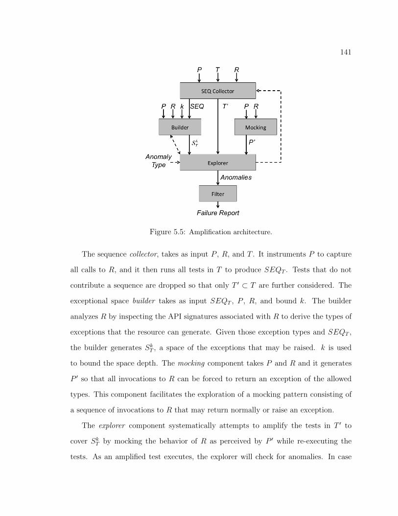
141

Figure 5.5: Amplification architecture.

The sequence collector, takes as input P , R, and T . It instruments P to capture

all calls to R, and it then runs all tests in T to produce SEQT . Tests that do not

contribute a sequence are dropped so that only T ′ ⊂ T are further considered. The

exceptional space builder takes as input SEQT , P , R, and bound k. The builder

analyzes R by inspecting the API signatures associated with R to derive the types of

exceptions that the resource can generate. Given those exception types and SEQT ,

the builder generates SkT , a space of the exceptions that may be raised. k is used

to bound the space depth. The mocking component takes P and R and it generates

P ′ so that all invocations to R can be forced to return an exception of the allowed

types. This component facilitates the exploration of a mocking pattern consisting of

a sequence of invocations to R that may return normally or raise an exception.

The explorer component systematically attempts to amplify the tests in T ′ to

cover SkT by mocking the behavior of R as perceived by P ′ while re-executing the

tests. As an amplified test executes, the explorer will check for anomalies. In case

142

where an anomaly is detected, the explorer will generate a trace of invocations to R

together with their outcome. The filter component will then take those anomalies

and report the ones meeting a predefined criteria such as whether to include amplified

tests whose mocking patterns and outcome were already revealed by other amplified

tests.

The description of the approach architecture overlooks some interesting aspects

that we have considered but not fully developed. First, in this work we pursue

exhaustive exploration of the space in ST . However, the architecture also allows more

selective exploration of the space to accommodate cost effectiveness tradeoffs. For

example, regular expressions could be provided to the builder to constrain the space

ST to specific exceptional patterns that are known to be problematic for a particular

system or resource.

Second, the dotted line from the explorer to the collector in Figure 5.5 alludes

to the potential for establishing a feedback loop where the new invocations of the

resources or the new outcomes of existing invocations revealed by the explorer are

used to enrich the ST .

Third, the dotted line between builder and explorer indicates that these processes

may be coupled so that the space is defined incrementally as it is being explored.

So the builder, for example, could define a space for one pattern and pass it to the

explorer, which in turn will influence the builder in the formation of the rest of ST .

This type of lazy space definition may be particularly effective at early stages of the

amplification where the size of the space is unknown.

Fourth, the types of anomalies considered could be extended by monitoring for

invocation of unexpected handlers due to exception inheritance, or exceptions that

are subsumed without proper handling. Such anomalies are often caused by inserting

empty handler blocks in the code, just to comply with compiler syntax checking, but

143

ignoring the important exceptions being raised.

Last, our architecture does not prescribe how the instrumentation and exploration

should occur. As we shall see, we use AspectJ to provide the mocking capability, but

other established frameworks, such as JMock[66] or EasyMock[35], could also be used,

and are discussed in Section 2.3.4.

5.3.4 Implementation

In this section we briefly describe the most interesting aspects of an implementation

of our approach in the context of Java 1.6 programs and JUnit test suites.

Collection and Mocking. We use AspectJ [116] 1.6.10 to instrument the artifacts

to collect SEQT , mock the API calls and inject exceptions, and to detect anomalies at

run time. Figure 5.6 shows an excerpt of the AspectJ point cut template we used. We

first define point cuts for the sites of the calls to the target resource APIs (Line 3). We

then define an advice that executes in place of the invocation of the call to the resource

API (Lines 6-14). The advice uses a pointer (currPtr) to track the exploration

progress. It calls method mockPatternPosition with currPtr as a parameter to

check whether to inject exception on the current invocation of the resource API, and

throws an exception if the check returns true, otherwise it executes the call normally.

The type of exception to be thrown is determined by a call to method mockExpType

with currPtr as a parameter. Both mockPatternPosition and mockExpType have

access to data structures that store the mocking patterns and the type of exceptions

to be thrown, which are generated automatically by the builder component.

Building and Exploration. Our builder and explorer work independently. First,

the builder analyzes the signatures of the methods in R invoked by P as indicated by

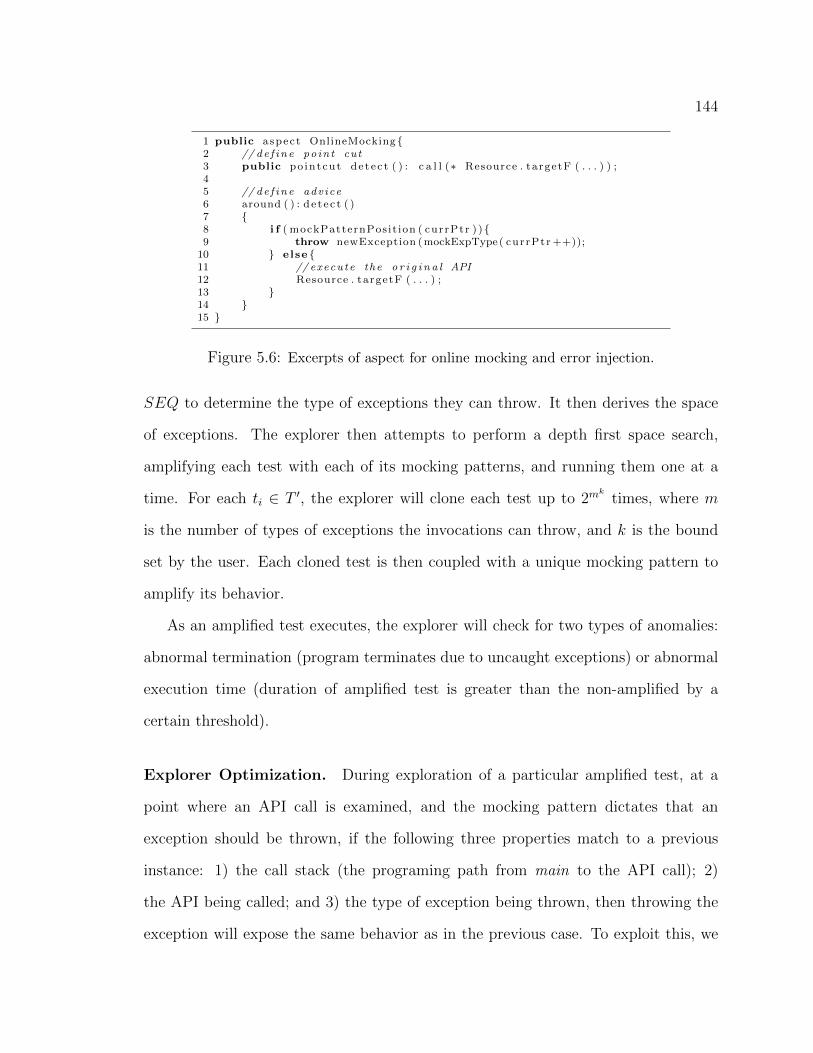
144

1 public aspect OnlineMocking{2 // de f ine po in t cut3 public po intcut de t e c t ( ) : c a l l (∗ Resource . targetF ( . . . ) ) ;45 // de f ine adv ice6 around ( ) : de t e c t ( )7 {8 i f ( mockPatternPosit ion ( currPtr ) ){9 throw newException (mockExpType( currPtr ++));

10 } else {11 // execute the o r i g i n a l API12 Resource . targetF ( . . . ) ;13 }14 }15 }

Figure 5.6: Excerpts of aspect for online mocking and error injection.

SEQ to determine the type of exceptions they can throw. It then derives the space

of exceptions. The explorer then attempts to perform a depth first space search,

amplifying each test with each of its mocking patterns, and running them one at a

time. For each ti ∈ T ′, the explorer will clone each test up to 2mktimes, where m

is the number of types of exceptions the invocations can throw, and k is the bound

set by the user. Each cloned test is then coupled with a unique mocking pattern to

amplify its behavior.

As an amplified test executes, the explorer will check for two types of anomalies:

abnormal termination (program terminates due to uncaught exceptions) or abnormal

execution time (duration of amplified test is greater than the non-amplified by a

certain threshold).

Explorer Optimization. During exploration of a particular amplified test, at a

point where an API call is examined, and the mocking pattern dictates that an

exception should be thrown, if the following three properties match to a previous

instance: 1) the call stack (the programing path from main to the API call); 2)

the API being called; and 3) the type of exception being thrown, then throwing the

exception will expose the same behavior as in the previous case. To exploit this, we

145

store a snapshot of the call stack of the test execution before each mocked exception,

and when executing another amplified test, at each point where an exception is to be

thrown, if the current call stack matches one of the stored snapshots, we skip exploring

the test any further, and move on to the next test. This strategy leads to performance

gains at the cost of sacrificing completeness. A match means throwing the exception

under consideration will not lead to any new exception handling behavior for this

instance of API call. However it is not guaranteed that the current amplified test

will not result in any new behavior in the future. In practice, as per our empirical

findings, the optimization did not miss any anomalies that was detected with the

un-optimized approach, and contributed to 5% - 12% savings in execution time of the

approach.

The Android Environment. Android applications compile into dex format (An-

droid bytecode) and execute on the Dalvik VM and the Android Virtual Device (AVD)

[6]. This imposes a challenge as we also want to run that code with AspectJ, which

requires a custom compiler to weave aspects into original class files. However, as As-

pectJ performs code injection on the bytecode level, and dex files (Android bytecode)

rely on class files, it is possible to adopt the following process: 1) Let Java compiler

compile Java code to class files; 2) Let AspectJ compiler (iajc) inject point cuts and

advices to class files; 3) Let Android code generator (dx) transform the new class files

and create dex files. We developed a custom Ant build script to automate the double

transformation process.

5.4 Evaluation

In this section we address the following research questions:

146

• RQ1: How cost effective are the amplified tests in detecting anomalies in ex-

ceptional handling code?

• RQ2: To what extent do the detected anomalies represent real faults?

5.4.1 Study Design and Implementation

We studied the Android applications and the resources listed in Table 5.1. For

each of those resources, we collected the checked exceptions that could be thrown

from public methods as defined by the Android SDK Specification [6] (i.e., for the

methods in android.bluetooth class, the included exceptions are ConnectionTime-

outException, SocketTimeoutException, UnknownHostException, for methods in an-

droid.database class, the included exceptions are CursorIndexOutOfBoundsException,

SQLException, StaleDataException, etc.). In total we identified 17 exception types

that could be thrown by the classes java.net, android.database, android.location and

android.bluetooth.

We set the approach parameters as follow. To set the approach mocking length

we mimic the process a tester would follow. Ideally a tester would select the smallest

mocking pattern length that still detects all the faults. This value, however, is not

known in advance, and it is different across programs, tests, and resources. So the

tester must pick a reasonable starting value that may be refined over time. Similarly,

we select a length of 10 which seems reasonable considering the time it takes to

explore the exceptional space of these applications. This decision also echoes with

Jackson’s small scope hypothesis [64] which conjectures that exhaustive testing up

to a small bound will detect most faults. As described next, our findings confirm

this hypothesis, as the majority of the faults can be detected with a length of 5.

To further explore the effect of mocking lengths on the effectiveness and efficiency

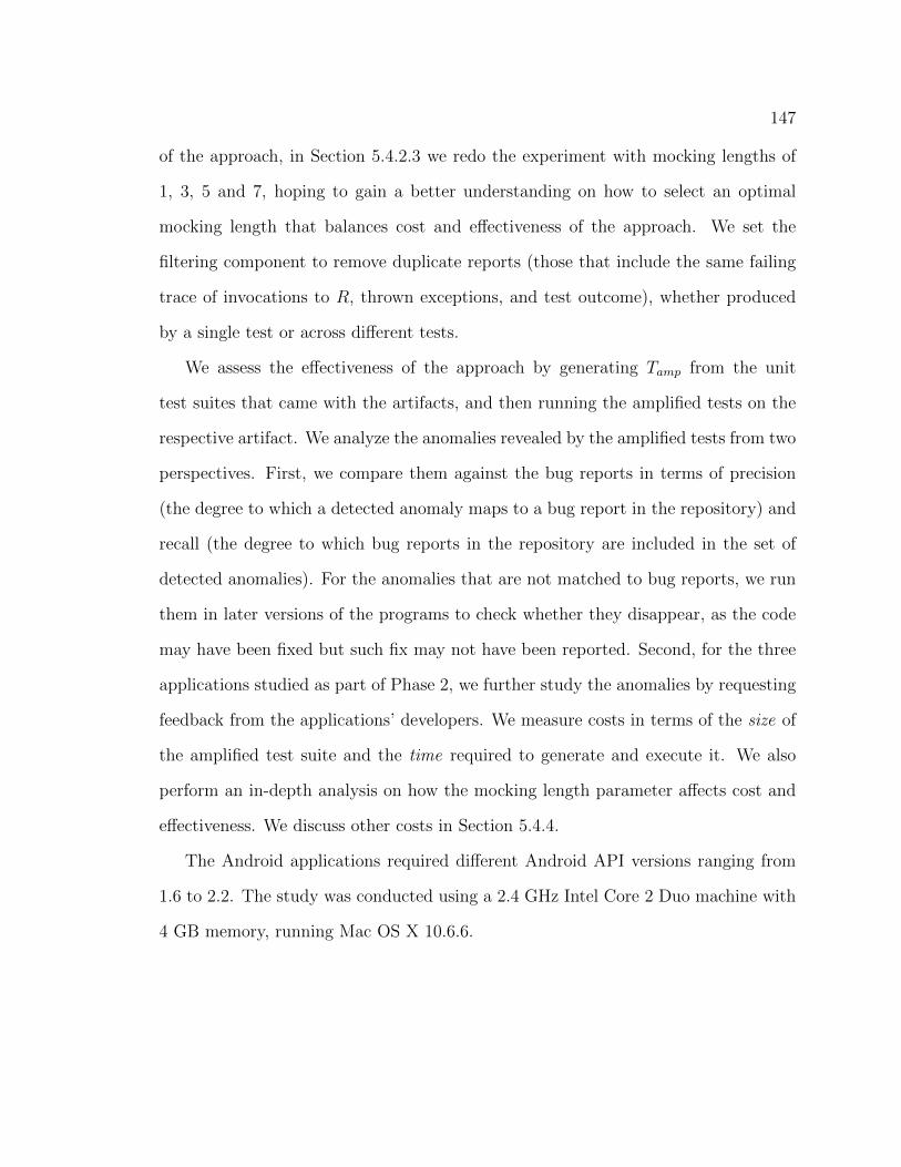
147

of the approach, in Section 5.4.2.3 we redo the experiment with mocking lengths of

1, 3, 5 and 7, hoping to gain a better understanding on how to select an optimal

mocking length that balances cost and effectiveness of the approach. We set the

filtering component to remove duplicate reports (those that include the same failing

trace of invocations to R, thrown exceptions, and test outcome), whether produced

by a single test or across different tests.

We assess the effectiveness of the approach by generating Tamp from the unit

test suites that came with the artifacts, and then running the amplified tests on the

respective artifact. We analyze the anomalies revealed by the amplified tests from two

perspectives. First, we compare them against the bug reports in terms of precision

(the degree to which a detected anomaly maps to a bug report in the repository) and

recall (the degree to which bug reports in the repository are included in the set of

detected anomalies). For the anomalies that are not matched to bug reports, we run

them in later versions of the programs to check whether they disappear, as the code

may have been fixed but such fix may not have been reported. Second, for the three

applications studied as part of Phase 2, we further study the anomalies by requesting

feedback from the applications’ developers. We measure costs in terms of the size of

the amplified test suite and the time required to generate and execute it. We also

perform an in-depth analysis on how the mocking length parameter affects cost and

effectiveness. We discuss other costs in Section 5.4.4.

The Android applications required different Android API versions ranging from

1.6 to 2.2. The study was conducted using a 2.4 GHz Intel Core 2 Duo machine with

4 GB memory, running Mac OS X 10.6.6.

148

5.4.2 RQ1: Cost Effectiveness in Detecting Anomalies

We study this research question by amplifying the unit tests that came with the

artifacts, executing them and analyzing the behaviors they expose. We start by pre-

senting the result with mocking length of 10 and discuss its effectiveness in exposing

anomalies. Then we will repeat the study with various decreasing mocking lengths to

explore its effect on the tradeoff between cost and effectiveness. Finally we present

a characterization of the mocking patterns that do expose anomalies, in the hope of

discovering certain patterns that are more effective in detecting anomalies.

5.4.2.1 Results with Mocking Length=10

We start by providing a characterization of the original test suite, T , in Table 5.3.

For each artifact-resource combination, we report the number of original tests ex-

ercising each one of the resources and the time required to execute them. We also

report coverage on the try-catch blocks that the original test suite achieved through

JMeter [59], with the assistant of a simple instrumentation that marks the try-catch

blocks in the source code. To facilitate a quicker comparison, in Column “# Original

Tests” we copied the number of tests in the original test suites associated with the

applications from Table 5.1. We note that the initial test screening process helped

to eliminate many original tests that do not reach the target exceptional constructs.

For example, for Barcode Scanner, just 18% of the original tests were able to exercise

the external resource android.net.

In Table 5.4, we provide a characterization of the amplified test suite, Tamp.

Columns “Amplification Time”, “# Tests Amplified”, and “Execution Time” columns

indicate the cost of amplifying the screened test suite (in seconds), the number of am-

plified tests and their execution times (in hours) respectively. For comparison reasons

we also include coverage on the try-catch blocks which are achieved by Tamp, and its

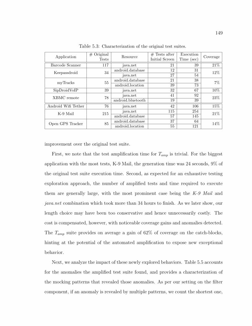
149

Table 5.3: Characterization of the original test suites.

Application# Original

Resource# Tests after Execution

CoverageTests Initial Screen Time (sec)

Barcode Scanner 117 java.net 21 39 21%

Keepassdroid 34android.database 12 31

12%java.net 27 54

myTracks 55android.database 21 38

7%android.location 39 73

SipDroidVoIP 39 java.net 32 67 10%

XBMC remote 78java.net 41 92

23%android.bluetooth 19 39

Android Wifi Tether 76 java.net 42 106 15%

K-9 Mail 215java.net 115 254

21%android.database 57 145

Open GPS Tracker 85android.database 37 64

14%android.location 55 121

improvement over the original test suite.

First, we note that the test amplification time for Tamp is trivial. For the biggest

application with the most tests, K-9 Mail, the generation time was 24 seconds, 9% of

the original test suite execution time. Second, as expected for an exhaustive testing

exploration approach, the number of amplified tests and time required to execute

them are generally large, with the most prominent case being the K-9 Mail and

java.net combination which took more than 34 hours to finish. As we later show, our

length choice may have been too conservative and hence unnecessarily costly. The

cost is compensated, however, with noticeable coverage gains and anomalies detected.

The Tamp suite provides on average a gain of 62% of coverage on the catch-blocks,

hinting at the potential of the automated amplification to expose new exceptional

behavior.

Next, we analyze the impact of these newly explored behaviors. Table 5.5 accounts

for the anomalies the amplified test suite found, and provides a characterization of

the mocking patterns that revealed those anomalies. As per our setting on the filter

component, if an anomaly is revealed by multiple patterns, we count the shortest one,

150

Table 5.4: Characterization of the amplified test suites.

Application ResourceAmplify # Amplified Execution Coverage

Time (sec) Tests Time (hrs) (gains)

Barcode Scanner java.net 17.1 17,921 10.1 81% (+60%)

Keepassdroidandroid.database 3.5 9,721 7.5

75% (+63%)java.net 6.8 18,856 17.3

myTracksandroid.database 5.9 17,734 14.3

81% (+74%)android.location 8.1 31,543 22.7

SipDroidVoIP java.net 6.2 24,476 17.6 74% (+64%)

XBMC remotejava.net 7.5 33,255 18.6

76% (+53%)android.bluetooth 5.4 16,547 9.5

Android Wifi Tether java.net 10.7 35,512 14.2 73% (+58%)

K-9 Mailjava.net 24.1 91,117 34.5

71% (+50%)android.database 11.4 40,623 11.4

Open GPS Trackerandroid.database 7.6 31,125 17.6

79% (+65%)android.location 12.3 44,258 21.3

which we deem easier for the user to trace the problem (the rest of the patterns are

ignored for all other counts). The amplified test suite identified 211 unique anomalies,

an average of 26 per application. Of those anomalies, 61% corresponded to mocking

patterns that consisted of more than a single throw in response to a call to the API.

This clearly shows that throwing more complex exceptions can greatly help detecting

anomalies. There are three anomalies (in XBMC remote, in Keepassdroid, and in K-9

Mail) that require mocking length of 10 to be detected. These three are infinite loops

which require an “All Throw” mocking pattern of length 10 to detect the issue. All

considered, we found that the average mocking pattern length to detect an anomaly

is just over 3, with 2 throws on average per pattern, indicating that the cost of the

approach could be drastically reduced by selecting a much tighter exploration bound.

5.4.2.2 Controlling the Mocking Length Parameter for Cost Effectiveness

To better convey the effects of the mocking pattern length on testing costs and fault

detection effectiveness, we repeated the study with mocking lengths 1, 3, 5 and 7.

Figure 5.7 shows the results of the study in each program and resource. In each

151

Table 5.5: Anomalies detected.

Application# Anomalies Mocking Pattern

Detected # More Than A Single Throw Avg Length Max Length

Barcode Scanner 19 9 (47%) 2.6 5

Keepassdroid11 9 (82%) 5.1 1018 10 (56%) 2.1 5

myTracks19 12 (63%) 3.4 59 5 (56%) 3.2 5

SipDroidVoIP 16 9 (56%) 1.9 4

XBMC remote14 8 (57%) 4.8 109 6 (67%) 3.1 4

Android Wifi Tether 10 10 (100%) 3.1 4

K-9 Mail39 19 (49%) 2.1 416 10 (63%) 2.1 10

Open GPS Tracker14 10 (71%) 3.2 517 11 (65%) 2.8 4

graph, there are five data points, corresponding to the results of executing one Tamp

generated with a distinctive mocking length (from left to right: 1, 3, 5, 7, and 10).

The X-axis corresponds to cost in terms of execution time in hours, and the Y-axis

corresponds to the number of anomalies found.

From all 13 graphs, we can observe a similar trend, in which the curve becomes

saturated as the the mocking length increases, but at different rates. Out of the 13

graphs, 10 reached saturation at mocking length of 5. For most programs, further

investment in amplifying testing resources does not translate into more detection

power. For the other three graphs (5.7(b), 5.7(g), 5.7(l)), the saturation point was

not reached, as increasing the mocking length still leads to the detection of more

anomalies. However, given enough testing resources (in this case, more test execution

time), they will become saturated, as the approach will exhaust all possible mocking

patterns eventually.

For all artifacts, Tamp generated with a mocking length of 1 detected only 2% of the

anomalies, as it did not explore a large part of the interesting exceptional behavior.

With a length of 5, 96% of the anomalies detected with a length of 10 were found

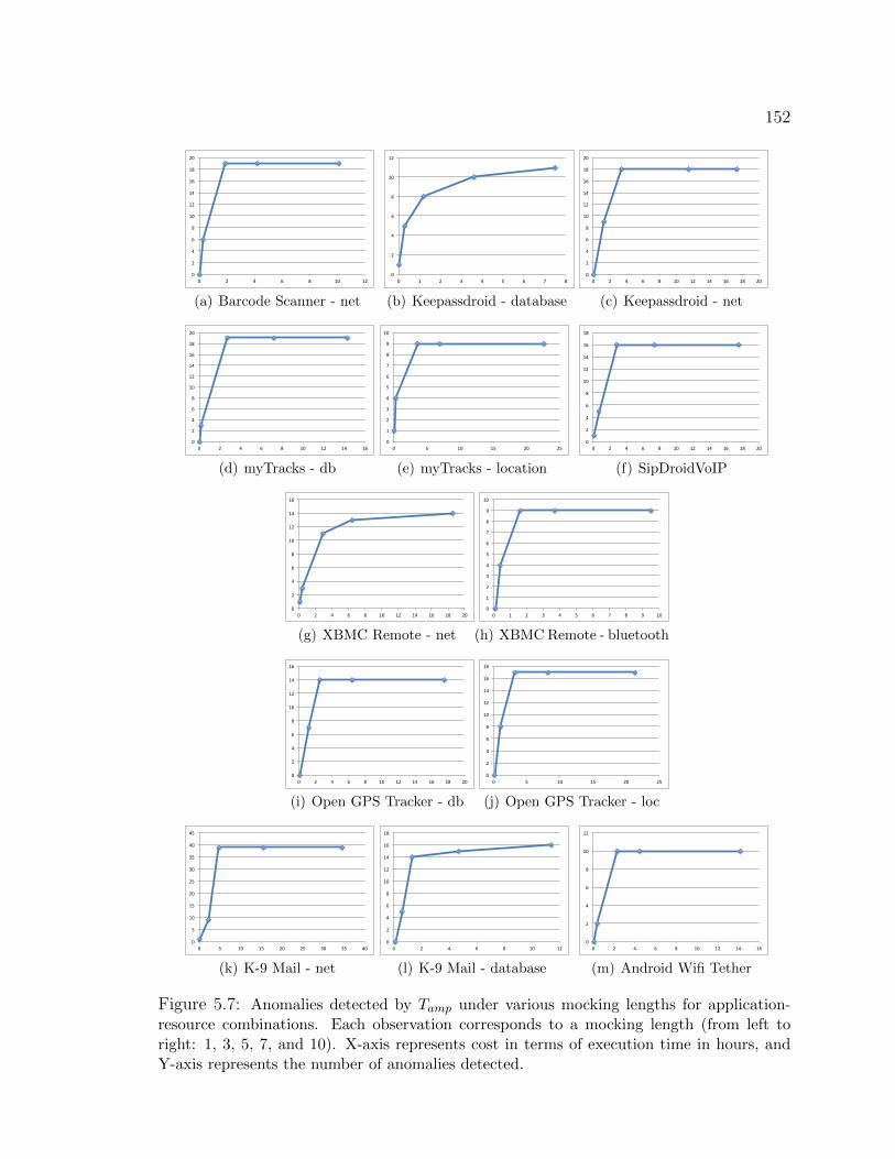
152

0

2

4

6

8

10

12

14

16

18

20

0 2 4 6 8 10 12

(a) Barcode Scanner - net

0

2

4

6

8

10

12

0 1 2 3 4 5 6 7 8

(b) Keepassdroid - database

0

2

4

6

8

10

12

14

16

18

20

0 2 4 6 8 10 12 14 16 18 20

(c) Keepassdroid - net

0

2

4

6

8

10

12

14

16

18

20

0 2 4 6 8 10 12 14 16

(d) myTracks - db

0

1

2

3

4

5

6

7

8

9

10

0 5 10 15 20 25

(e) myTracks - location

0

2

4

6

8

10

12

14

16

18

0 2 4 6 8 10 12 14 16 18 20

(f) SipDroidVoIP

0

2

4

6

8

10

12

14

16

0 2 4 6 8 10 12 14 16 18 20

(g) XBMC Remote - net

0

1

2

3

4

5

6

7

8

9

10

0 1 2 3 4 5 6 7 8 9 10

(h) XBMC Remote - bluetooth

0

2

4

6

8

10

12

14

16

0 2 4 6 8 10 12 14 16 18 20

(i) Open GPS Tracker - db

0

2

4

6

8

10

12

14

16

18

0 5 10 15 20 25

(j) Open GPS Tracker - loc

0

5

10

15

20

25

30

35

40

45

0 5 10 15 20 25 30 35 40

(k) K-9 Mail - net

0

2

4

6

8

10

12

14

16

18

0 2 4 6 8 10 12

(l) K-9 Mail - database

0

2

4

6

8

10

12

0 2 4 6 8 10 12 14 16

(m) Android Wifi Tether

Figure 5.7: Anomalies detected by Tamp under various mocking lengths for application-resource combinations. Each observation corresponds to a mocking length (from left toright: 1, 3, 5, 7, and 10). X-axis represents cost in terms of execution time in hours, andY-axis represents the number of anomalies detected.

153

with less than 5% of the cost. Overall these results confirm that our choice of 10 as

the default mocking length is indeed conservative. It also shows the flexibility of our

approach. In situations where testing resources are limited, a tester can use a smaller

mocking length, while retaining most of the detection powers of the tool. However, it

is worth noting that a bound of 5 would have missed 8 anomalies that corresponded

to faults in Keepassdroid, XBMC remote and K-9 Mail, so the savings may come at a

cost for some artifacts. As discussed previously, in certain cases, there are anomalies

that can only be detected by patterns of length 10 (like the three instances of infinite

loops).

5.4.2.3 A Closer Look at the Mocking Patterns

To better understand the role of the mocking patterns in detecting these anomalies, we

analyze the mocking patterns that effectively detected anomalies in the previous study

with mocking length of 10. We categorize the patterns in the following categories: 1)

Single Throw - 1st, in which only the first instance of the API call throws an exception,

and all the other instances return normally; 2) All Throw, in which all instances of API

invocations throw exceptions; 3) Single Throw - not 1st, in which only one instance of

the API invocation throws an exception, but its location in the sequence of API calls

can be anywhere except the first instance; 4) Multi Throw - One Transition, in which

multiple instances of the API calls can throw exceptions, but there can only be one

transition either from non-throwing to throwing, or vice versa; for example, a pattern

of three throws followed by 2 normal returns falls into this category; 5) Multi Throw

- Multi Transition, in which multiple instances of the API calls can throw exceptions,

and multiple transitions occur as well. For example, a pattern of intermittent throw

/ normal execution falls into this category. The first two categories, Single Throw -

1st and All Throw, are most likely supported by existing frameworks (e.g. the Eclipse

154

4 3

76

49

79

0 10 20 30 40 50 60 70 80 90

single throw

-‐ 1st

all throw

single throw

-‐ not 1st

mul; throw -‐ one transi;on

mul; throw -‐ m

ul; transi;on

# anomalies

Figure 5.8: Categorization of mocking patterns.

IDE for Android application development provides support for mocking of APIs that

can be configured to throw a single exception or throw exceptions at all times). The

third category, which represents instances of one arbitrary exception being thrown,

is often used in manual test cases for exception handling code. The fourth and fifth

categories, which correspond to patterns that describe intermittent resource on/offs

over a period of time, are unlikely to be used in existing testing processes or tools.

The results (Figure 5.8) show that the majority (97%) of the anomalies are in

fact detected by the more complex patterns in the last three categories. Patterns in

the category of Multi Throw - Multi Transition detected the most anomalies. This

shows that intermittent patterns, in which throw and normal returns are interleaved,

are most effective in detecting anomalies. These data explains, at least in part, why

manual test cases often fail to detect bugs in exception handling code. Without an

exhaustive testing approach it is difficult for a tester to come up with the complex

155

patterns that do expose bugs of this type.

In summary, investigation of RQ1 suggests that an amplified test suite can pro-

vide significant coverage gains of exception handling code, detect many anomalies in

existing popular applications, and do so through the exploration of patterns that are

non-trivial. We now proceed to investigate these anomalies.

5.4.3 RQ2: Anomalies & Failures

We now assess whether the anomalies we found contributed to real faults. We strike at

RQ2 from two perspectives. First, we compare the anomalies found by the approach

against the bug reports of the applications in terms of precision and recall. For

the anomalies that are not matched to bug reports, we execute the amplified tests

that revealed them on the newest version of the applications, evaluating whether

the anomalies are still present. We conjecture that if the anomalies are not present,

that means that code revisions removed them in the new versions, thus they were

potential real faults. Second, for the three applications studied as part of Phase 2,

we further study the anomalies by seeking feedback from the application developers

for confirmation, and then report their comments.

5.4.3.1 Precision and Recall

We start the assessment of the detected anomalies by mapping them to real bug

reports. We compute the percentage of bug reports associated with the anomalies

found and the percentage of anomalies that are included in the bug reports. The first

metric gives us a notion of the approach completeness (also refer to as recall) while

the second provides a lower bound on the approach preciseness. We note that both

metrics are inherently limited (e.g., they assume that all faults have been found and

that all found faults have a bug report) but they are useful to pinpoint strengths and

156

weaknesses of the approach.

The process to map anomalies to bug reports is as follows. First, we search among

the bug repository for instances of the location (call to target API or exception) where

an anomaly was detected. If the resulting bug report includes a stack trace, which

is often the case, we will match it with the stack trace associated with the anomaly.

Otherwise, we retrieve the submitted fix to the bug, and inspect the code to determine

if the fix was applied to the ill coded exception handling module that was captured

by the anomaly reported by the amplified test.

Out of the 211 detected anomalies, 137 of them are matched to bug reports. The

other 74 anomalies may be false positives, or they may correspond to real faults

that are yet to be reported. To investigate this possibility, we run the 74 amplified

tests that detected these anomalies on the newest version of the applications. If

the anomalies are not present, that means that code revisions removed them as the

applications evolve, thus they could have been real faults. For the five applications

from Phase 1, the new versions corresponds to the latest version available on June

2011. For the three newly added applications, the new versions corresponds to that

of October 2012.

In this step, 27 out of the 74 remaining anomalies that appear in older versions are

not present in the latest versions, which adds credibility to the value of the anomalies

detected by the approach. We also note that the 47 remaining anomalies are induced

by amplified tests with more complex mocking patterns, with an average length of

3.6, as compared to the amplified tests that detected all 211 anomalies, which had an

average mocking pattern length of 3.1. This result may indicate that the remaining

anomalies represent faults that are harder to find.

Figure 5.9 combines the results from the previous steps. Each bar represents the

total number of anomalies detected by the amplified suite for one artifact, and the

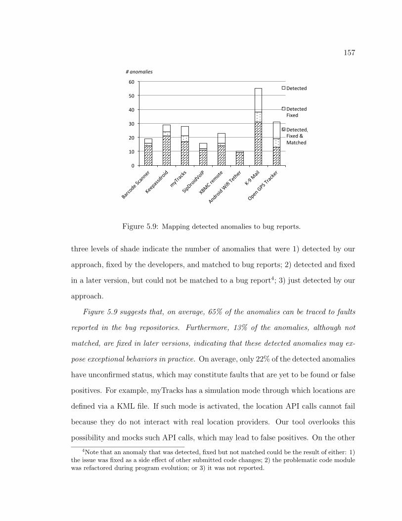
157

0

10

20

30

40

50

60

Barcode Scanner

Keepassdroid

myTracks

SipDroidVoIP

XBMC remote

Android Wifi Tether

K-‐9 Mail

Open GPS Tracker

Detected

Detected & Fixed

Detected, Fixed & Matched

# anomalies

Figure 5.9: Mapping detected anomalies to bug reports.

three levels of shade indicate the number of anomalies that were 1) detected by our

approach, fixed by the developers, and matched to bug reports; 2) detected and fixed

in a later version, but could not be matched to a bug report4; 3) just detected by our

approach.

Figure 5.9 suggests that, on average, 65% of the anomalies can be traced to faults

reported in the bug repositories. Furthermore, 13% of the anomalies, although not

matched, are fixed in later versions, indicating that these detected anomalies may ex-

pose exceptional behaviors in practice. On average, only 22% of the detected anomalies

have unconfirmed status, which may constitute faults that are yet to be found or false

positives. For example, myTracks has a simulation mode through which locations are

defined via a KML file. If such mode is activated, the location API calls cannot fail

because they do not interact with real location providers. Our tool overlooks this

possibility and mocks such API calls, which may lead to false positives. On the other

4Note that an anomaly that was detected, fixed but not matched could be the result of either: 1)the issue was fixed as a side effect of other submitted code changes; 2) the problematic code modulewas refactored during program evolution; or 3) it was not reported.

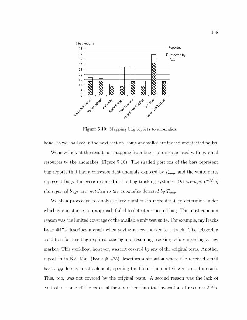
158

0 5 10 15 20 25 30 35 40 45

Barcode Scanner

Keepassdroid

myTracks

SipDroidVoIP

XBMC remote

Android Wifi Tether

K-‐9 Mail

Open GPS Tracker

Reported

Detected by

# bug reports

Tamp

Figure 5.10: Mapping bug reports to anomalies.

hand, as we shall see in the next section, some anomalies are indeed undetected faults.

We now look at the results on mapping from bug reports associated with external

resources to the anomalies (Figure 5.10). The shaded portions of the bars represent

bug reports that had a correspondent anomaly exposed by Tamp, and the white parts

represent bugs that were reported in the bug tracking systems. On average, 67% of

the reported bugs are matched to the anomalies detected by Tamp.

We then proceeded to analyze those numbers in more detail to determine under

which circumstances our approach failed to detect a reported bug. The most common

reason was the limited coverage of the available unit test suite. For example, myTracks

Issue #172 describes a crash when saving a new marker to a track. The triggering

condition for this bug requires pausing and resuming tracking before inserting a new

marker. This workflow, however, was not covered by any of the original tests. Another

report in in K-9 Mail (Issue # 475) describes a situation where the received email

has a .gif file as an attachment, opening the file in the mail viewer caused a crash.

This, too, was not covered by the original tests. A second reason was the lack of

control on some of the external factors other than the invocation of resource APIs.

159

For example, myTracks issue #137 describes a bug where the user gets many error

messages when trying to upload tracks to the Google Maps service. Reproducing the

bug requires controlling two factors: a Google authentication API that fails all the

time, and a specific scheduling order for two threads. Our approach controls the first

factor, but does not have control over the second.

While the first shortcoming can be addressed by devoting more testing efforts,

the second issue requires extending our approach to include a more sophisticated

instrumentation mechanism to capture and replay the threads schedule.

5.4.3.2 Feedback From Application Developers

According to Figure 5.9, there are 56 (26%) anomalies whose status cannot be de-

termined. Treating them as false positive is to our disadvantage because we suspect

that some of them may correspond to real faults that are yet to be reported, thus

we cannot find a match in the bug repository. In order to further investigate these

anomalies, we sent some of them to the applications’ developers, asking them to

examine the anomalies, and provide feedback to either confirm or reject our findings.

The process is as follows. First, we selected the three newly added applications

Open GPS Tracker, K-9 Mail and Android Wifi Tether, because their high level

of recent activities made us believe it is more likely to reach the right developers.

The three applications have 30 anomalies whose status is undecided (12 for Open

GPS Tracker, 17 for K-9 Mail and 1 for Android Wifi Tether). We decided to send

a sample of these anomalies to the developers in order to increase our chances of

getting feedback from them. We randomly selected three anomalies from Open GPS

Tracker, three from K-9 Mail and the one from Android Wifi Tether, for a total of

seven anomalies. Second, we contacted the developers, explaining our intent. Once

they agreed to participate, we sent them materials to familiarize them with our tool

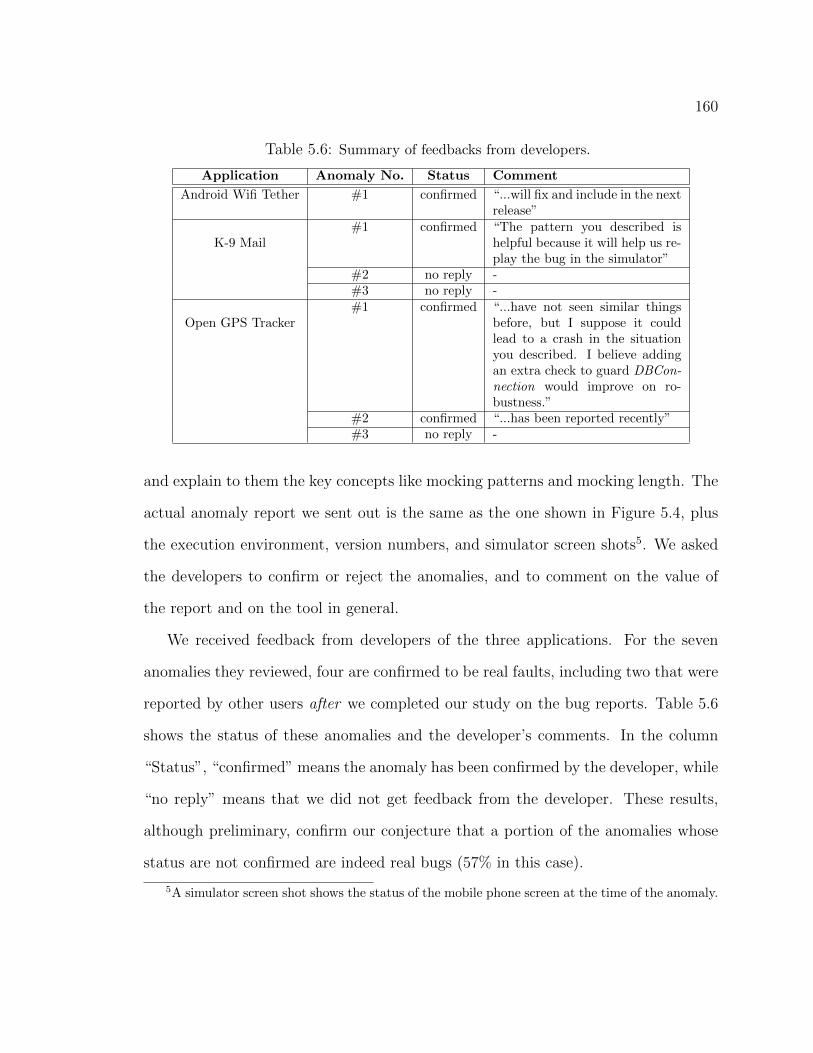
160

Table 5.6: Summary of feedbacks from developers.

Application Anomaly No. Status Comment

Android Wifi Tether #1 confirmed “...will fix and include in the nextrelease”

K-9 Mail#1 confirmed “The pattern you described is

helpful because it will help us re-play the bug in the simulator”

#2 no reply -#3 no reply -

Open GPS Tracker#1 confirmed “...have not seen similar things

before, but I suppose it couldlead to a crash in the situationyou described. I believe addingan extra check to guard DBCon-nection would improve on ro-bustness.”

#2 confirmed “...has been reported recently”#3 no reply -

and explain to them the key concepts like mocking patterns and mocking length. The

actual anomaly report we sent out is the same as the one shown in Figure 5.4, plus

the execution environment, version numbers, and simulator screen shots5. We asked

the developers to confirm or reject the anomalies, and to comment on the value of

the report and on the tool in general.

We received feedback from developers of the three applications. For the seven

anomalies they reviewed, four are confirmed to be real faults, including two that were

reported by other users after we completed our study on the bug reports. Table 5.6

shows the status of these anomalies and the developer’s comments. In the column

“Status”, “confirmed” means the anomaly has been confirmed by the developer, while

“no reply” means that we did not get feedback from the developer. These results,

although preliminary, confirm our conjecture that a portion of the anomalies whose

status are not confirmed are indeed real bugs (57% in this case).

5A simulator screen shot shows the status of the mobile phone screen at the time of the anomaly.

161

5.4.4 Threats to Validity

In addition to the limitations we mentioned in Section 5.1 regarding the scope of the

programs we studied and the potentially noisy nature of analyzing bug reports, we

introduced some other threats in this section. More specifically, our choice of versions

was deliberate to maximize the number of faults that could be detected. In practice,

the deltas will be smaller and is not certain how the collected metrics will be affected.

Second, the metrics we utilized are just partial proxies for the cost effectiveness of

the approach and are highly context dependent. In a more realistic setting, the cost

of the approach would also include the time required by developers to interpret the

tool’s outputs and exclude the false positives. Third, our focus was on particular

types of exceptions that we deemed interesting based on our experience. Although

the approach is applicable to other exception handling constructs and resources, its

cost effectiveness may vary according to the difficulties associated with particular the

resources. Fourth, our study on developer feedback was preliminary and focused only

on three developers and a subset of the detected anomalies.

5.4.5 Extended Domain and Alternative Approach

In this section we briefly compare the proposed approach against the CAR-Miner

tool developed by Thummalapenta et al. [117]. This tool represents one of the latest

attempts targeting the detection of errors in exception handling code. Instead of

amplifying or generating a test suite, CAR-Miner mines exception handling rules

from the source code of a pool of applications and then checks whether a target

program violates those rules.

Our comparison with CAR-Miner is focused on HsqlDB, the artifact on which

CAR-Miner detected the most faults [117]. HsqlDB is a database application with

162

almost 30KLoc in version 1.7.1 (the one used in the original study) and 551 unit

tests. We take advantage of the public availability of this application to examine its

bug reports as we did for the Android applications in Section 5.1. The examination,

which was conducted in summer of 2010, found 178 confirmed bug reports that led

to code revisions. Among them, 58 (32%) were caused by poorly handled exceptions

and 14 were caused by the external resource java.db (the core external resource used

by this application). This seems to indicate that the proper handling of exceptions

in HsqlDB is as challenging as for the Android applications, but the effect of external

resources is smaller as the Android applications seem to rely more heavily on external

sensors and communication services.

CAR-Miner detected 51 instances of broken rules in HsqlDB and the authors were

able to map 10 of those to bug reports. Upon closer examination we noticed that three

of those bug reports were later rejected by the developers, which leaves CAR-Miner

with seven broken rules that map to reported bugs. One of these three instances,

#1896443 is particularly interesting because it points to one of the limitations of this

type of approaches in their analysis scope. The use of intraprocedural analysis means

that longer exception handling patterns are often missed.

Amplifying the HsqlDB test suite with our approach resulted in 97,280 amplified

tests that take 19.4 hours to execute and find 22 anomalies. Among the anomalies

found are the 7 confirmed faults found by CAR-Miner, and two other faults from the

repository. One such instance, bug report #1800705, shows a case where a raised ex-

ception caused a DB connection not to close properly. Again, because the exception

is not thrown by an explicit API call in the method but rather by a chain of exception

re-throws that propagated a lower level exception to the current method, CAR-Miner

is not able to detect it. In terms of false positives, as expected, the mining approach

reported over 85% of false positives (51 anomalies reported from which 7 were con-

163

firmed faults). For our approach, the same criteria gives a false positive rate of 59%

(9 of 22 were confirmed bugs).

5.4.6 Preliminary Case Study

To start addressing some of the limitations we identified in terms of the scope of the

work and its lack of development context, we performed an initial case study of the

approach assisting Android applications developers. Our case study was conducted in

the convenient context of BusLinc [22], an application for the Android platform being

developed by a team of senior Computer Science students at University of Nebraska-

Lincoln, two professional Android developers, and the IT division of the Lincoln

StarTran transportation service. The application communicates with StarTran’s lo-

cation server and, combined with a smartphone’s current location, can provide users

detailed bus route, nearest bus stop, and real-time bus schedule information.

The application primarily uses two types of resource APIs, a network API that

communicates with a server, and a location API that is used to obtain the device

physical location. We use our approach to assist with the testing of exception handling

behaviors of the network API, which was used more extensively than the location API.

We generated 2048 amplified tests based on just two automated system tests provided

by the developers. In 20 minutes the approach reported 4 distinct anomalies, all of

which were terminations caused by poorly handled exceptions, and involved non-

trivial mocking patterns whose lengths range between 2 and 4.

One such anomaly reflected a situation where the network communication suc-

ceeded in checking server availability and route updates, but failed at retrieving the

actual bus routes. Consequently, the route object was stored as a null pointer and a

subsequent reference to the object crashed the application. Two other anomalies of

similar type were detected, one for checking out the bus stops, the other for vehicles.

164

The last anomaly was associated with the logic for displaying a route on the Google

Maps overlay, where the waypoints on the route were null objects due to a network

failure in updating them.

We met with two of the student developers to gain further insights on these anoma-

lies. During the meeting, the developers were directed towards the code locations with

the poorly implemented exception handlers that caused the crashes, and were asked

to construct failing scenarios for the network API usage that could lead to these

crashes. After 15 minutes, the developers failed to identify scenarios for any of the

four failures. We then provided and explained the failure reports. With those at hand,

the developers recognized and confirmed the problems. Based on these preliminary

findings, it seems that the approach was useful in revealing non-obvious problems

with their exception handling constructs.

5.5 Summary

In this chapter we have introduced a simple yet cost effective approach aimed at am-

plifying existing tests to validate exception handling code associated with external

resources. The technical merit of the approach resides in defining the challenge as

a coverage problem over the space of potential exceptional behavior, and the sys-

tematic manipulation of the environment to cover that space. Although our focus

was motivated by faults triggered by noisy and unreliable external resources, the ap-

proach could be beneficial in other scenarios where there is limited understanding or

confidence on an API.

The findings of our studies indicate that amplified suites are powerful enough to

detect over 200 anomalies, the majority (97%) of which are detected under complex

mocking patterns. These anomalies eventually led to code fixes 65% of the time and

165

included 78% of the reported bugs. Our approach outperforms a state of the art

approach in precision and recall. In addition, the feedback from developers and the

preliminary case study illustrate the approach’s potential to assist developers.

166

Chapter 6

Conclusions and Future Work

In this chapter, we first summarize the techniques presented in Chapters 3 to 5.

We then identify the limitations of these techniques, and discuss possible solutions

on how to overcome the limitations. In the end, we conclude this dissertation by

identifying several areas of future work that are related to our research on non-

functional validation.

6.1 Summary and Impact

In this dissertation, we presented several techniques that enable cost-effective vali-

dation of non-functional software requirements. Specifically, we targeted two aspects

of non-functional testing. For non-functional requirements defined as qualities of a

system, we targeted validation of performance properties. There are many existing

techniques that target performance validation, however, they do not provide support

for choosing the critical values that expose worst cases, but focusing on increasing

size and rate of input, which is a rather expensive way of inducing load, and may

lead to negligence of real performance faults. We improved cost effectiveness of per-

formance validation by automatically generating load tests that focus on smart input

167

value selection to expose worst case performance scenarios in diverse ways. We subse-

quently introduced a compositional load test generation technique that targeted more

complex software systems, to which the previous technique failed to scale. For non-

functional requirements defined as constraints on a system, we targeted contextual

constraints on noisy and unreliable external resources with which a software system

must interact. One way to improve robustness of software is to use exception handling

constructs. In practice, however, the code handling exceptions is not only difficult

to implement but also challenging to validate. We improved the cost effectiveness of

such validation by amplifying existing tests to exhaustively test every possible pat-

tern in which exceptions can be raised, and produce scenarios in which the exception

handling code does not hold.

Automatic Load Test Generation. In Chapter 3, we presented SLG, an ap-

proach that automatically generates load test suites by performing a focused form

of symbolic execution. Symbolic execution, being a white box exhaustive technique,

provides many benefits to load test generation. It can potentially generate load tests

that target input values that can expose worst case behaviors. Furthermore, because

symbolic execution exhaustively traverses all program paths, it can also lead to a test

suite that loads the system in diverse ways. To improve scalability, SLG considers

program paths in phases. Within each phase it performs an exhaustive exploration.

At the end of each phase, the paths are grouped based on similarity, and the most

promising path from each group, relative to the consumption measure, is selected to

explore in the next phase.

We implemented SLG on top of the Symbolic Path Finder framework, and assessed

its cost effectiveness on three real world Java applications: JZlib (5633 LOC), a data

compression application; SAT4J (10731 LOC), a SAT solver; and TinySQL (8431

168

LOC), a database management system. Our assessment of SLG shows that it can

induce program loads across different types of resources that are significantly better

than alternative approaches (randomly generated tests in the case of JZlib, a standard

benchmark in the case SAT4J, and the default suite in the the case of TinySQL).

Furthermore, we provide evidence that the approach scales to inputs of large size and

complexity and produces functionally diverse test suites.

For more complex software systems on which SLG failed to scale, in Chapter 4 we

presented CompSLG, a technique that generate load tests compositionally, using SLG

as a subroutine in its own analysis. CompSLG uses SLG to analyze the performance

of each system component in isolation, summarizes the results of those analyses, and

then performs an analysis across those summaries to generate load tests for the whole

system. We have presented novel approaches to solve 1) how to generate channeling

constraints, which are key to connect constraint systems of different components;

2) how path constraints across components must be weighted and relaxed in order

to derive test inputs for the whole system while ensuring that the most significant

constraints, in terms of inducing load, are enforced.

CompSLG is fully automated to handle any Java system that is structured in the

form of a software pipeline. A study of CompSLG revealed that it can generate load

tests for Unix and XML pipelines where SLG alone would not scale up, and it is much

more cost effective than either SLG applied to single components or Random test

generation. We also investigated how to extend CompSLG to enable its application

to Java programs, in which each method considered is a component, resulting in a

much more complex structure than a pipeline. The extension includes a new approach

to generating channeling constraints, generating performance summaries with more

precise metadata, and an adapted strategy for composing summaries. Although the

extended version is not yet fully implemented, we showed the viability of the approach

169

with several proof-of-concept examples.

For years techniques and tools for performance validation or characterization have

treated the target program as a black box. We are among the first to advocate and

develop a more precise technique for such activities, and the outcome of this research

provides efficient solutions that solve this fundamental problem. We believe our notion

of compositional analysis in generating test cases is also inspirational to researchers

aiming to scale symbolic execution based techniques.

Validation of Exception Handling Code. In Chapter 5, we presented an auto-

mated technique to support the detection of faults in exception handling code that

deals with external resources. The technique was motivated by the idea of small

scope hypothesis [64], which stated that many faults could be exposed by perform-

ing a bounded number of program operations, and that by doing so exhaustively no

corner cases are missed. The technique is simple, scalable, and effective in practice

when combined with a test suite that invokes the resources of interest. The approach

first instruments the target program so that the results of calls to external resources

of interest can be mocked at will to return exceptions. Then, existing test cases are

systematically amplified by re-executing them on the instrumented program under

various mocked patterns to explore the space of exceptional behavior. When an am-

plified test reveals a fault, the mocking pattern applied with the test serves as an

explanation of the failure induced by the external resource. To control the number

of amplified tests the approach prunes tests with duplicate calls and call-outcomes

to the external resources, and bounds the number of calls that define the space of

exceptional behavior explored.

The technique was assessed on a set of eight Android mobile apps, and the findings

of our studies indicate that the technique is powerful enough to detect over 200

170

anomalies, the majority (97%) of which are detected under complex mocking patterns.

These anomalies eventually led to code fixes 65% of the time and included 78% of the

reported bugs. Our approach also outperforms a state of the art approach in terms

of precision and recall. In addition, the feedback from developers and a preliminary

case study illustrate the approachs potential to assist developers.

This technique was the first in the software testing field to transform the problem

of exception handling code validation into the established area of search space explo-

ration, and the first to use the idea of bounded exhaustive testing to solve it. Our

modeling of external resource as patterns could illuminate future research in related

areas.

6.2 Limitations

In this section, we identify key limitations to the techniques presented in Chapters 3-

5. Generally, there are two types of limitations: limitations caused by the design of

a technique, and limitations caused by the implementation of a technique. Table 6.1

summarizes both types of limitations, which we discusses in detail below.

Limitations in Symbolic Load Generation (SLG). For the Symbolic Load

Generation (SLG) technique presented in Chapter 3, the key limitation by design is

the selection of the values for parameters of the technique, such as the lookAhead

parameter that controls how much distance the search advances in each iteration of

iterative-deepening, and the maxSolverConstraints parameter, which determines how

many constraints to collect before calling the solver in CLLG. As stated in Chapter 3,

the lookAhead parameter is essential in controlling the efficiency of the SLG algorithm,

and the maxSolverConstraints is used to balance the tradeoff between the quality of

the generated tests and the scalability of the CLLG algorithm. The existing technique

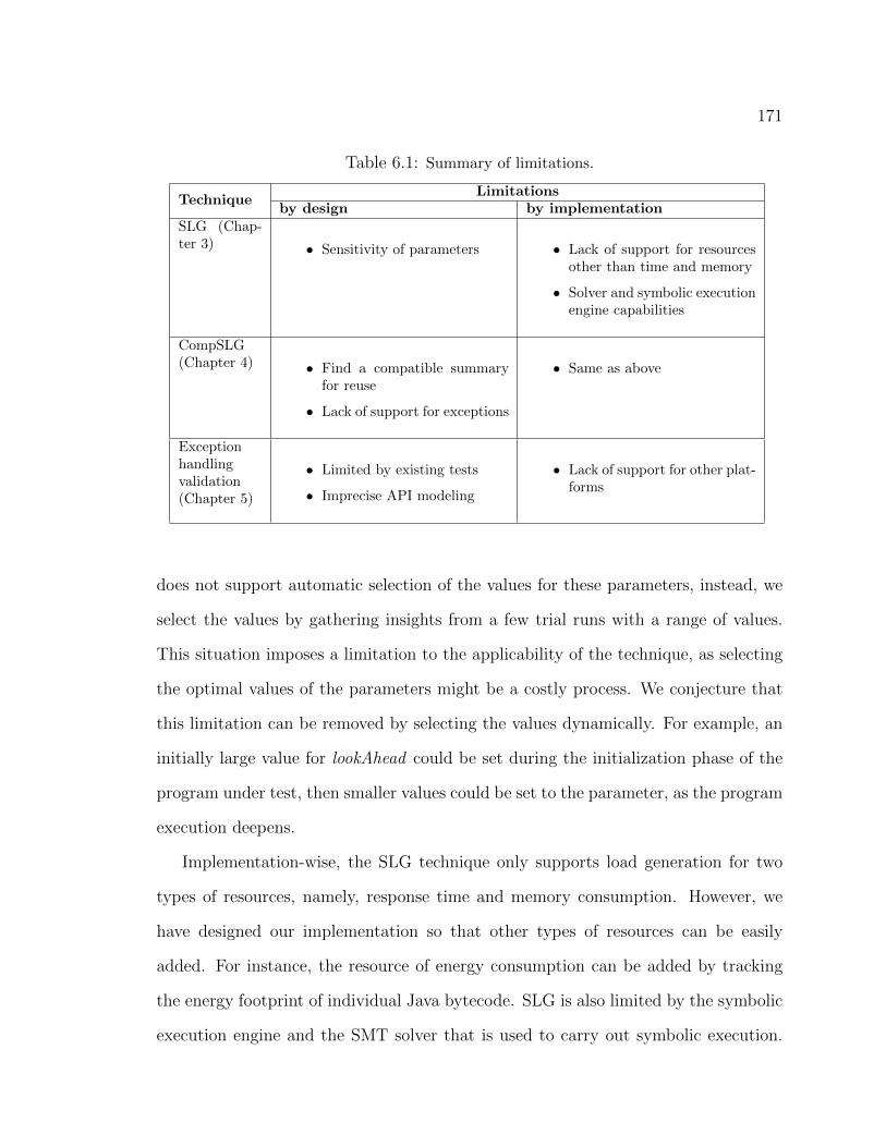
171

Table 6.1: Summary of limitations.

TechniqueLimitations

by design by implementationSLG (Chap-ter 3) • Sensitivity of parameters • Lack of support for resources

other than time and memory

• Solver and symbolic executionengine capabilities

CompSLG(Chapter 4) • Find a compatible summary

for reuse

• Lack of support for exceptions

• Same as above

Exceptionhandlingvalidation(Chapter 5)

• Limited by existing tests

• Imprecise API modeling

• Lack of support for other plat-forms

does not support automatic selection of the values for these parameters, instead, we

select the values by gathering insights from a few trial runs with a range of values.

This situation imposes a limitation to the applicability of the technique, as selecting

the optimal values of the parameters might be a costly process. We conjecture that

this limitation can be removed by selecting the values dynamically. For example, an

initially large value for lookAhead could be set during the initialization phase of the

program under test, then smaller values could be set to the parameter, as the program

execution deepens.

Implementation-wise, the SLG technique only supports load generation for two

types of resources, namely, response time and memory consumption. However, we

have designed our implementation so that other types of resources can be easily

added. For instance, the resource of energy consumption can be added by tracking

the energy footprint of individual Java bytecode. SLG is also limited by the symbolic

execution engine and the SMT solver that is used to carry out symbolic execution.

172

This limitation can be relieved by incorporating more powerful engines and solvers

to the technique.

Limitations in Compositional Load Generation (CompSLG). For the Comp-

SLG technique presented in Chapter 4, there are two key limitations introduced by

the design of the technique. First, as presented in Section 4.6.2, a precise summary

(such as the one that preserves the shape of input/output objects) can lead to a pre-

cise compositional analysis, which ultimately leads to better load inducing test suites.

However, keeping precise summaries may countermine the savings achieved through

a compositional analysis, as the technique may not be able to find a matching sum-

mary from the library, instead, it is forced to generate a new summary that matches

the particular specification. We conjecture two directions that can help overcome

this limitation. On one hand, the technique should provide a flexible definition that

allows various levels of approximations for the performance summary. Depending

on the complexity of the program under test, the technique may choose to produce

summaries on different levels of approximation suitable for the situation. On the

other hand, in case that a precise summary matching cannot be achieved, the tech-

nique should provide a mechanism that allows a broader selection of summaries to

be reused. For example, in bubbleSort, if a matching summary, which has an input

of 1001 integers, cannot be found in the library, but a summary that has an input of

1000 integers is present in the library, the technique can reuse the one 1000 integers in

place for the one with 1001 integers. Similar reusing mechanisms can also be applied

to summaries that preserve shape of input / output objects. Note that this selection

will lead to an under-approximation in the analysis, which may have implications for

the quality of the generated tests.

Second, the CompSLG technique for Java programs does not consider the presence

173

of exceptions that can be thrown at runtime by the program under test. When an

exception is thrown, the program will take alternative execution paths that cannot be

encoded solely by constraints on the symbolic input variables. It is also possible that

a load-inducing execution path is the one with the presence of exceptions. For exam-

ple, a path that repeatedly encounters network connection exceptions and repeatedly

tries to reconnect can be an expensive path in terms of response time. To enable

CompSLG to generate this type of test cases, we need to 1) update the definition of

the performance summary to allow encoding of exception throwing patterns, in addi-

tion to the constraints on the symbolic input variables; 2) use an updated control flow

graph that features exception control flow edges to guide the compositional analysis.

Limitations in exception handling code validation. For the exception vali-

dation technique presented in Chapter 5, there are two key limitations caused by

the design of the technique. First, the exception handling behavior exposed by the

amplified test suite is limited by the coverage of the original test suite. As shown

in Section 5.4.3, if the original test suite misses certain regions of the code, the am-

plified test suite is likely to miss the same region. This limitation can be relieved

by establishing a feedback loop where the new invocations of the resources revealed

by amplifying the existing test cases can be used to enrich the pool of tests to be

amplified, which in turn will lead to more behavior coverage by the technique.

Second, the technique for exception testing is built as an exhaustive approach.

It is shown to be an effective technique, but the cost of applying it is high. For

example, in our study presented in Chapter 5, the cost of applying the technique

to Android apps ranges from 4 hours to 24 hours, depending on the size of the

original test suite, the mocking length, and the complexity of the program under

test. We plan to investigate the interplay between the technique and real world usage

174

rules of the external resources, which may help inform what mocking patterns are

worth exploring, thus enabling a more selective exploration instead of an exhaustive

approach. For example, when an Android app runs without access to data connection,

the app may use certain mechanism to reroute database queries to locally cached data,

instead of submitting the queries online. As a result, certain types of exceptions, such

as SQLiteException, could not occur in reality. Our current implementation ignores

this situation and incorrectly mocks the full behavior. To overcome this limitation we

will leverage the usage rules of the APIs to eliminate this type of over-approximation.

6.3 Future Work

In this section, we identify several areas of future work related to our research on

non-functional validation. We first describe a few directions towards improving the

proposed techniques. We then present a few long term research goals that involve

pushing a more precise and scalable non-functional validation both to the millions of

desktop programmers, and to the cloud computing systems.

Extension of CompSLG to richer structures. In Chapter 4 we presented an

extension of CompSLG that enables load test generation for Java programs. In its

current form, this extension is largely manual, and requires a non-trivial implemen-

tation to be fully automated. Our first goal is to automate this proposed technique,

and to assess it on a rich set of applications.

In the long term, we also plan to investigate different automatic software de-

composition techniques. The cost effectiveness of the compositional load generation

technique is affected by how the system under test is decomposed. Much work has

been done on automatic software decomposition, with various focuses on testing [25],

visualization [15], and maintenance [53]. We plan to create our own flavor of software

175

decomposition with a focus on how it will make it easier for load generation technique

to analyze it later on.

Seamless non-functional test generation in the IDE. For desktop program-

ming, it is predicted that the steady improvements in automatic test case generation,

software bug finding, and code verification techniques will make it far easier for a

programmer in the future to quickly write software that is reliable, maintainable, and

malleable [96]. In a few years, the advances in computational power will enable IDEs

to run constantly as many relevant tests as possible all the time while the programmer

is working [97]. This will provide nearly instant feedback when semantic bugs arise.

As part of future work, we propose to build the technology that enables such

instant feedback on non-functional properties of the code. To achieve this goal, we

plan to test waters by first integrating the load generation technique into the Eclipse

IDE. It will be deployed as an early warning system, constantly generating load test

cases for the available code, and raising flags for abnormalities such as excessive CPU

or memory usage. The challenges for building this technology involves 1) significantly

speedup the current test generation techniques to match the expectations of seamless

continuous test generation paradigm; and 2) intuitively reduce false positives to avoid

overwhelming the user with false error messages.

Load testing in the cloud. The popularity of cloud computing in recent years

has provided cost effective ways of scaling expensive computations. As part of future

work, we propose to speedup the non-functional test generation techniques presented

in this dissertation by utilizing cloud computing powers. Towards this goal, the

following aspects must be considered 1) how to adapt the existing algorithms so that

a trade-off between communication overhead and accuracy of path selection heuristic

can be achieved; and 2) how to balance load among worker nodes.

176

From a different perspective, performance is an important requirement for appli-

cations in the cloud. In extreme cases, near real-time responsiveness is preferred on

services such as banking fraud detection, etc. Despite this, the performance of a cloud

system is always evaluated with benchmarks that either use random or predefined in-

put data [135]. Running on an heterogeneous environment, knowing what type of

workload would expose worst case performance scenarios for a cloud system is very

important for a system engineer to estimate the potential of the system he manages.

Our load generation technique can be extended to enable generating workloads for

such systems. To achieve this, factors that have not been considered, such as network

latency, disk access latency, and data locality, have to be explicitly considered when

deriving new methods.

177

Bibliography

[1] A. A. Abdelaziz, W. M. W. Kadir, and A. Osman. Article:Comparative Analysis

of Software Performance Prediction Approaches in Context of Component-based

System. International Journal of Computer Applications, 23(3):15–22, June

2011. Published by Foundation of Computer Science.

[2] M. Acharya and T. Xie. Mining API Error-Handling Specifications from Source

Code. In Proceedings of the 12th International Conference on Fundamental Ap-

proaches to Software Engineering: Held as Part of the Joint European Con-

ferences on Theory and Practice of Software, ETAPS 2009, FASE ’09, pages

370–384. Springer-Verlag, 2009.

[3] S. Anand, P. Godefroid, and N. Tillmann. Demand-driven Compositional Sym-

bolic Execution. In Proceedings of the Theory and Practice of Software, 14th

International Conference on Tools and Algorithms for the Construction and

Analysis of Systems, TACAS’08/ETAPS’08, pages 367–381. Springer-Verlag,

2008.

[4] S. Anand, C. S. Pasareanu, and W. Visser. Symbolic Execution with Abstrac-

tion. International Journal on Software Tools Technology Transfer, 11(1):53–67,

Jan. 2009.

[5] Android-aspectj tool. http://code.google.com/p/android-aspectj/, 2011.

178

[6] Android developers doc. http://developer.android.com/index.html.

[7] Android open source db. http://www.aopensource.com/.

[8] Android wifi tether code host. http://code.google.com/p/

myandroid-wifi-tether/, 2012.

[9] Androlib website. http://www.androlib.com/appstats.aspx, 2012.

[10] S. Artzi, A. Kiezun, J. Dolby, F. Tip, D. Dig, A. Paradkar, and M. D. Ernst.

Finding Bugs in Dynamic Web Applications. In Proceedings of the 2008 In-

ternational Symposium on Software Testing and Analysis, ISSTA ’08, pages

261–272. ACM, 2008.

[11] A. Avritzer and E. J. Weyuker. The Automatic Generation of Load Test Suites

and the Assessment of the Resulting Software. IEEE Transactions on Software

Engineering, 21(9):705–716, Sept. 1995.

[12] S. Balsamo, A. Di Marco, P. Inverardi, and M. Simeoni. Model-Based Perfor-

mance Prediction in Software Development: A Survey. IEEE Transactions on

Software Engineering, 30(5):295–310, May 2004.

[13] L. Bass, P. Clements, and R. Kazman. Software Architecture in Practice.

Addison-Wesley Longman Publishing Co., Inc., 1998.

[14] M. Bayan and J. a. W. Cangussu. Automatic Feedback, Control-based, Stress

and Load Testing. In Proceedings of the 2008 ACM Symposium on Applied

Computing, SAC ’08, pages 661–666. ACM, 2008.

[15] D. Beyer. CCVisu: Automatic Visual Software Decomposition. In Companion

of the 30th International Conference on Software Engineering, ICSE Companion

’08, pages 967–968. ACM, 2008.

179

[16] J. M. Bieman, D. Dreilinger, and L. Lin. Using Fault Injection to Increase Soft-

ware Test Coverage. In Proceedings of the The Seventh International Symposium

on Software Reliability Engineering, ISSRE ’96, pages 166–. IEEE Computer

Society, 1996.

[17] G. Bolch, S. Greiner, H. de Meer, and K. Trivedi. Queueing Networks and

Markov Chains: Modeling and Performance Evaluation with Computer Science

Applications. Wiley-Interscience, 1998.

[18] C. Boyapati, S. Khurshid, and D. Marinov. Korat: Automated Testing based

on Java Predicates. In Proceedings of the 2002 ACM SIGSOFT International

Symposium on Software Testing and Analysis, ISSTA ’02, pages 123–133. ACM,

2002.

[19] G. Bradski. The OpenCV Library. Dr. Dobb’s Journal of Software Tools, 2000.

[20] J. Burnim, S. Juvekar, and K. Sen. WISE: Automated Test Generation for

Worst-case Complexity. In Proceedings of the 31st International Conference on

Software Engineering, ICSE ’09, pages 463–473. IEEE Computer Society, 2009.

[21] R. P. Buse and W. R. Weimer. Automatic Documentation Inference for Excep-

tions. In Proceedings of the 2008 International Symposium on Software Testing

and Analysis, ISSTA ’08, pages 273–282. ACM, 2008.

[22] Buslinc code host. http://code.google.com/p/android-unl2011/.

[23] C. Cadar, D. Dunbar, and D. Engler. KLEE: Unassisted and Automatic Gener-

ation of High-coverage Tests for Complex Systems Programs. In Proceedings of

the 8th USENIX Conference on Operating Systems Design and Implementation,

OSDI’08, pages 209–224. USENIX Association, 2008.

180

[24] C. Cadar, V. Ganesh, P. M. Pawlowski, D. L. Dill, and D. R. Engler. EXE:

Automatically Generating Inputs of Death. In Proceedings of the 13th ACM

Conference on Computer and Communications Security, CCS ’06, pages 322–

335. ACM, 2006.

[25] A. Chakrabarti and P. Godefroid. Software Partitioning for Effective Auto-

mated Unit Testing. In Proceedings of the 6th ACM & IEEE International

Conference on Embedded Software, EMSOFT ’06, pages 262–271. ACM, 2006.

[26] Choco solver. http://www.emn.fr/x-info/choco-solver/doku.php.

[27] J.-D. Choi, D. Grove, M. Hind, and V. Sarkar. Efficient and Precise Modeling

of Exceptions for the Analysis of Java Programs. SIGSOFT Softw. Eng. Notes,

24(5):21–31, Sept. 1999.

[28] E. Coppa, C. Demetrescu, and I. Finocchi. Input-sensitive Profiling. In Proceed-

ings of the 33rd ACM SIGPLAN Conference on Programming Language Design

and Implementation, PLDI ’12, pages 89–98. ACM, 2012.

[29] D. Coppit, J. Yang, S. Khurshid, W. Le, and K. J. Sullivan. Software Assurance

by Bounded Exhaustive Testing. IEEE Transactions on Software Engineering,

31(4):328–339, 2005.

[30] Cvc3 solver website. http://www.cs.nyu.edu/acsys/cvc3/.

[31] Cyrket mobile app statistics. http://www.cyrket.com/m/android/.

[32] B. Daniel, D. Dig, K. Garcia, and D. Marinov. Automated Testing of Refac-

toring Engines. In Proceedings of the the 6th Joint Meeting of the European

Software Engineering Conference and the ACM SIGSOFT Symposium on The

181

foundations of Software Engineering, ESEC-FSE ’07, pages 185–194. ACM,

2007.

[33] L. De Moura and N. Bjørner. Z3: an Efficient SMT Solver. In Pro-

ceedings of the Theory and Practice of Software, 14th International Confer-

ence on Tools and Algorithms for the Construction and Analysis of Systems,

TACAS’08/ETAPS’08, pages 337–340. Springer-Verlag, 2008.

[34] R. Dechter. Constraint Processing. Morgan Kaufmann Publishers Inc., 2003.

[35] Easymock website. http://easymock.org/.

[36] Eclipse bug 362718 - workbench performance tests. https://bugs.eclipse.

org/bugs/show_bug.cgi?id=362718.

[37] Eclipse bug repository. https://bugs.eclipse.org/bugs/.

[38] S. Elbaum, H. N. Chin, M. B. Dwyer, and M. Jorde. Carving and Replaying

Differential Unit Test Cases from System Test Cases. IEEE Transactions on

Software Engineering, 35:29–45, January 2009.

[39] M. Emmi, R. Majumdar, and K. Sen. Dynamic Test Input Generation for

Database Applications. In Proceedings of the 2007 International Symposium on

Software Testing and Analysis, ISSTA ’07, pages 151–162. ACM, 2007.

[40] D. Farmer and E. H. Spafford. The COPS Security Checker System, 1994.

[41] S. Freeman, T. Mackinnon, N. Pryce, and J. Walnes. Mock Roles, Objects. In

Companion to the 19th annual ACM SIGPLAN Conference on Object-oriented

Programming Systems, Languages, and Applications, OOPSLA ’04, pages 236–

246. ACM, 2004.

182

[42] S. Freeman and N. Pryce. Evolving an Embedded Domain-specific Language in

Java. In Companion to the 21st ACM SIGPLAN Symposium on Object-oriented

Programming Systems, Languages, and Applications, OOPSLA ’06, pages 855–

865. ACM, 2006.

[43] S. Frolund and J. Koistinen. QML: A Language for Quality of Service Specifi-

cation. Technical Report 10, HP Laboratories, 1998.

[44] C. Fu and B. G. Ryder. Exception-Chain Analysis: Revealing Exception Han-

dling Architecture in Java Server Applications. In Proceedings of the 29th Inter-

national Conference on Software Engineering, ICSE ’07, pages 230–239. IEEE

Computer Society, 2007.

[45] C. Fu, B. G. Ryder, A. Milanova, and D. Wonnacott. Testing of Java Web Ser-

vices for Robustness. In Proceedings of the 2004 ACM SIGSOFT International


2004.

[46] V. Ganesh and D. L. Dill. A Decision Procedure for Bit-vectors and Arrays. In

Proceedings of the 19th International Conference on Computer Aided Verifica-

tion, CAV’07, pages 519–531. Springer-Verlag, 2007.

[47] I. Ghosh, N. Shafiei, G. Li, and W.-F. Chiang. JST: an Automatic Test Gen-

eration Tool for Industrial Java Applications with Strings. In Proceedings of

the 2013 International Conference on Software Engineering, ICSE ’13, pages

992–1001. IEEE Press, 2013.

[48] M. Glinz. Rethinking the Notion of Non-Functional Requirements. In in Pro-

ceedings of the Third World Congress for Software Quality (3WCSQ’05, pages

55–64, 2005.

183

[49] P. Godefroid. Compositional Dynamic Test Generation. In Proceedings of the

34th Annual ACM SIGPLAN-SIGACT Symposium on Principles of Program-

ming Languages, POPL ’07, pages 47–54. ACM, 2007.

[50] P. Godefroid, A. Kiezun, and M. Y. Levin. Grammar-based Whitebox Fuzzing.

In Proceedings of the 2008 ACM SIGPLAN Conference on Programming Lan-

guage Design and Implementation, PLDI ’08, pages 206–215. ACM, 2008.

[51] P. Godefroid, N. Klarlund, and K. Sen. DART: Directed Automated Random

Testing. In Proceedings of the 2005 ACM SIGPLAN Conference on Program-

ming Language Design and Implementation, PLDI ’05, pages 213–223. ACM,

2005.

[52] S. F. Goldsmith, A. S. Aiken, and D. S. Wilkerson. Measuring Empirical Com-

putational Complexity. In Proceedings of the the 6th Joint Meeting of the Eu-

ropean Software Engineering Conference and the ACM SIGSOFT Symposium

on The Foundations of Software Engineering.

[53] R. Gopal and S. Schach. Using Automatic Program Decomposition Techniques

in Software Maintenance Tools. In Software Maintenance, 1989., Proceedings.,

Conference on, pages 132–141, 1989.

[54] S. L. Graham, P. B. Kessler, and M. K. Mckusick. Gprof: A Call Graph Exe-

cution Profiler. In Proceedings of the 1982 SIGPLAN Symposium on Compiler

Construction, SIGPLAN ’82, pages 120–126. ACM, 1982.

[55] M. Grechanik, C. Fu, and Q. Xie. Automatically Finding Performance Problems

with Feedback-directed Learning Software Testing. In Proceedings of the 2012

International Conference on Software Engineering, ICSE 2012, pages 156–166.

IEEE Press, 2012.

184

[56] A. Groce and W. Visser. Model Checking Java Programs Using Structural

Heuristics. In Proceedings of the 2002 ACM SIGSOFT International Symposium

on Software Testing and Analysis, ISSTA ’02, pages 12–21. ACM, 2002.

[57] D. Grove, G. DeFouw, J. Dean, and C. Chambers. Call Graph Construction in

Object-oriented Languages. In Proceedings of the 12th ACM SIGPLAN Confer-

ence on Object-oriented Programming, Systems, Languages, and Applications,

OOPSLA ’97, pages 108–124. ACM, 1997.

[58] S. Gulwani, K. K. Mehra, and T. Chilimbi. SPEED: Precise and Efficient Static

Estimation of Program Computational Complexity. In Proceedings of the 36th

Annual ACM SIGPLAN-SIGACT Symposium on Principles of Programming

Languages, POPL ’09, pages 127–139. ACM, 2009.

[59] E. Halili. Apache JMeter. Packt Publishing, 2008.

[60] S. Han, Y. Dang, S. Ge, D. Zhang, and T. Xie. Performance Debugging in

the Large via Mining Millions of Stack Traces. In Proceedings of the 2012

International Conference on Software Engineering, ICSE 2012, pages 145–155.

IEEE Press, 2012.

[61] J. A. Hartigan and M. A. Wang. Algorithm AS 136: A K-Means Clustering

Algorithm. Journals of the Royal Statistical Society, pages 100–108, 1979.

[62] H. Hermanns, U. Herzog, and J. P. Katoen. Process Algebra for Performance

Evaluation. Theory of Computer Science, 274(1-2):43–87, 2002.

[63] G. Hughes and T. Bultan. Interface Grammars for Modular Software Model

Checking. In Proceedings of the 2007 International Symposium on Software

Testing and Analysis, ISSTA ’07, pages 39–49. ACM, 2007.

185

[64] D. Jackson and C. Damon. Elements of Style: Analyzing a Software Design

Feature with a Counterexample Detector. IEEE Transactions on Software En-

gineering, 22(7):484–495, 1996.

[65] Java path finder website. http://babelfish.arc.nasa.gov/trac/jpf.

[66] Jmock framework. http://www.jmock.org/index.html.

[67] Jshell. http://geophile.com/jshell/.

[68] Junitperf website. http://www.clarkware.com/software/JUnitPerf.html.

[69] Jzlib website. http://www.jcraft.com/jzlib/.

[70] K-9 mail code host. http://code.google.com/p/k9mail/, 2012.

[71] Keepassdroid code host. http://code.google.com/p/keepassdroid/, 2011.

[72] S. Khurshid, C. S. Pasareanu, and W. Visser. Generalized Symbolic Execution

for Model Checking and Testing. In Proceedings of the 9th International Con-

ference on Tools and Algorithms for the Construction and Analysis of Systems,

TACAS’03, pages 553–568. Springer-Verlag, 2003.

[73] J. C. King. Symbolic Execution and Program Testing. Communications of

ACM, 19(7):385–394, July 1976.

[74] C. Lattner and V. Adve. LLVM: A Compilation Framework for Lifelong Pro-

gram Analysis & Transformation. In Proceedings of the International Sympo-

sium on Code Generation and Optimization: Feedback-directed and Runtime

Optimization, CGO ’04, pages 75–. IEEE Computer Society, 2004.

186

[75] S. Lauterburg, A. Sobeih, D. Marinov, and M. Viswanathan. Incremental State-

space Exploration for Programs with Dynamically Allocated Data. In Proceed-

ings of the 30th International Conference on Software Engineering, ICSE ’08,

pages 291–300. ACM, 2008.

[76] Y. C. Law, J. H. Lee, and B. M. Smith. Automatic Generation of Redun-

dant Models for Permutation Constraint Satisfaction Problems. Constraints,

12(4):469–505, Dec. 2007.

[77] Le wiki koumbit: Open source android applications. https://wiki.koumbit.

net/AndroidFreeSoftware.

[78] M. H. Liffiton and K. A. Sakallah. Algorithms for Computing Minimal Unsat-

isfiable Subsets of Constraints. J. Autom. Reason., 40(1):1–33, Jan. 2008.

[79] Load test tools. http://www.softwareqatest.com/qatweb1.html.

[80] Loadunit website. http://loadunit.sourceforge.net.

[81] R. Majumdar and R.-G. Xu. Directed Test Generation Using Symbolic Gram-

mars. In Proceedings of the 22nd IEEE/ACM International Conference on

Automated Software Engineering, ASE ’07, pages 134–143. ACM, 2007.

[82] M. Mannion and B. Keepence. SMART requirements. SIGSOFT Software

Engineering Notes, 20(2):42–47, Apr. 1995.

[83] D. Michie. “Memo”: Functions and Machine Learning. Nature, 218(1-2):19–22,

1968.

[84] mytracks code host. http://code.google.com/p/mytracks/, 2011.

187

[85] N. Nethercote and J. Seward. Valgrind: a Framework for Heavyweight Dynamic

Binary Instrumentation. In Proceedings of the 2007 ACM SIGPLAN Conference

on Programming Language Design and Implementation, PLDI ’07, pages 89–

100. ACM, 2007.

[86] Open gps tracker code host. http://code.google.com/p/open-gpstracker/,

2012.

[87] Open street map wiki. http://wiki.openstreetmap.org/wiki/Android#

OpenSource.

[88] Oracle application environment testing. http://www.

oracle.com/us/products/consulting/resource-library/

application-environment-testing-ds-1900126.pdf.

[89] Perftestplus website. http://www.perftestplus.com/load.htm.

[90] C. S. Pasareanu, N. Rungta, and W. Visser. Symbolic Execution with Mixed

Concrete-symbolic Solving. In Proceedings of the 2011 International Symposium

on Software Testing and Analysis, ISSTA ’11, pages 34–44. ACM, 2011.

[91] C. S. Pasareanu and W. Visser. A Survey of New Trends in Symbolic Execu-

tion for Software Testing and Analysis. Int. J. Softw. Tools Technol. Transf.,

11(4):339–353, Oct. 2009.

[92] C. S. Pasareanu, P. C. Mehlitz, D. H. Bushnell, K. Gundy-Burlet, M. Lowry,

S. Person, and M. Pape. Combining Unit-level Symbolic Execution and System-

level Concrete Execution for Testing NASA Software. In Proceedings of the 2008

International Symposium on Software Testing and Analysis, ISSTA ’08, pages

15–26. ACM, 2008.

188

[93] C. V. Ramamoorthy and H. F. Li. Pipeline Architecture. ACM Comput. Surv.,

9(1):61–102, Mar. 1977.

[94] T. Reps and G. Rosay. Precise Interprocedural Chopping. In Proceedings of

the 3rd ACM SIGSOFT Symposium on Foundations of Software Engineering,

SIGSOFT ’95, pages 41–52. ACM, 1995.

[95] M. P. Robillard and G. C. Murphy. Static Analysis to Support the Evolu-

tion of Exception Structure in Object-oriented Systems. ACM Transactions on

Software Engineering Methodology, 12(2):191–221, Apr. 2003.

[96] D. Saff and M. D. Ernst. Reducing Wasted Development Time via Continu-

ous Testing. In Proceedings of the 14th International Symposium on Software

Reliability Engineering, ISSRE ’03, pages 281–. IEEE Computer Society, 2003.

[97] D. Saff and M. D. Ernst. Continuous Testing in Eclipse. In Proceedings of

the 27th International Conference on Software Engineering, ICSE ’05, pages

668–669. ACM, 2005.

[98] M. Sama, S. G. Elbaum, F. Raimondi, D. S. Rosenblum, and Z. Wang. Context-

Aware Adaptive Applications: Fault Patterns and Their Automated Identifica-

tion. IEEE Transactions on Software Engineering, 36(5):644–661, 2010.

[99] Sat competition website. http://www.satcompetition.org/.

[100] Sat4j website. http://www.sat4j.org/.

[101] Z. Segall, D. Vrsalovic, D. Siewiorek, D. Yaskin, J. Kownacki, J. Barton,

R. Dancey, A. Robinson, and T. Lin. FIAT-fault Injection based Automated

Testing Environment. In Fault-Tolerant Computing, 1988. FTCS-18, Digest of

Papers., Eighteenth International Symposium on, pages 102–107, 1988.

189

[102] K. Sen, D. Marinov, and G. Agha. CUTE: a Concolic Unit Testing Engine for

C. In Proceedings of the 10th European Software Engineering Conference held

jointly with 13th ACM SIGSOFT International Symposium on Foundations of

Software Engineering, ESEC/FSE-13, pages 263–272. ACM, 2005.

[103] J. Seward and N. Nethercote. Using Valgrind to Detect Undefined Value Errors

with Bit-precision. In Proceedings of the Annual Conference on USENIX Annual

Technical Conference, ATEC ’05, pages 2–2. USENIX Association, 2005.

[104] D. Shannon, I. Ghosh, S. Rajan, and S. Khurshid. Efficient Symbolic Execution

of Strings for Validating Web Applications. In Proceedings of the 2nd Interna-

tional Workshop on Defects in Large Software Systems: Held in conjunction

with the ACM SIGSOFT International Symposium on Software Testing and

Analysis (ISSTA 2009), DEFECTS ’09, pages 22–26. ACM, 2009.

[105] E. Sherman, M. B. Dwyer, and S. Elbaum. Saturation-based Testing of Con-

current Programs. In Proceedings of the the 7th joint meeting of the European

Software Engineering Conference and the ACM SIGSOFT Symposium on the

Foundations of Software Engineering, ESEC/FSE ’09, pages 53–62. ACM, 2009.

[106] J. Shi, M. B. Cohen, and M. B. Dwyer. Integration Testing of Software Product

Lines Using Compositional Symbolic Execution. In Proceedings of the 15th

International Conference on Fundamental Approaches to Software Engineering,

FASE’12, pages 270–284. Springer-Verlag, 2012.

[107] N. Siegmund, S. S. Kolesnikov, C. Kastner, S. Apel, D. Batory, M. Rosenmuller,

and G. Saake. Predicting Performance via Automated Feature-interaction De-

tection. In Proceedings of the 2012 International Conference on Software Engi-

neering, ICSE 2012, pages 167–177. IEEE Press, 2012.

190

[108] Silk performer. http://microfocus.com/products/SilkPerformer.

[109] S. Sinha and M. J. Harrold. Analysis and Testing of Programs with Exception

Handling Constructs. IEEE Transactions on Software Engineering, 26(9):849–

871, Sept. 2000.

[110] S. Sinha, A. Orso, and M. J. Harrold. Automated Support for Development,

Maintenance, and Testing in the Presence of Implicit Control Flow. In Proceed-

ings of the 26th International Conference on Software Engineering, ICSE ’04,

pages 336–345. IEEE Computer Society, 2004.

[111] Sipdroidvoip code host. http://code.google.com/p/sipdroid/, 2011.

[112] Smallx. http://code.google.com/p/smallx/.

[113] C. Smith and L. Williams. Performance Solutions: a Practical Guide to Cre-

ating Responsive, Scalable Software. Addison Wesley Longman Publishing Co.,

Inc., 2002.

[114] Spec. http://www.spec.org/cpu2000/CINT2000/164.gzip/docs/164.gzip.

[115] D. Taylor. Teach Yourself Unix System Administration in 24 Hours. Sams

Publishing, 2003.

[116] The aspectj project website. http://www.eclipse.org/aspectj/.

[117] S. Thummalapenta and T. Xie. Mining Exception-handling Rules as Sequence

Association Rules. In Proceedings of the 31st International Conference on Soft-

ware Engineering, ICSE ’09, pages 496–506. IEEE Computer Society, 2009.

[118] S. Thummalapenta, T. Xie, N. Tillmann, J. de Halleux, and Z. Su. Synthesizing

Method Sequences for High-coverage Testing. In Proceedings of the 2011 ACM

191

international conference on Object oriented programming systems languages and

applications, OOPSLA ’11, pages 189–206. ACM, 2011.

[119] N. Tillmann and J. De Halleux. Pex: White Box Test Generation for .NET. In

Proceedings of the 2nd International Conference on Tests and Proofs, TAP’08,

pages 134–153. Springer-Verlag, 2008.

[120] Tinysql website. http://www.jepstone.net/tinySQL/.

[121] Trac: Open source android applications. http://trac.osuosl.org/trac/

replicant/wiki/ListOfKnownFreeApps.

[122] W. Visser, C. S. Pasareanu, and R. Pelanek. Test Input Generation for Java

Containers Using State Matching. In Proceedings of the 2006 International


2006.

[123] Report on Average Web Page Size. http://www.websiteoptimization.com/

speed/tweak/average-web-page/.

[124] W. Weimer and G. C. Necula. Mining Temporal Specifications for Error De-

tection. In Proceedings of the 11th International Conference on Tools and Al-

gorithms for the Construction and Analysis of Systems, TACAS’05, pages 461–

476. Springer-Verlag, 2005.

[125] Wikipedia: List of open source android applications. http://en.wikipedia.

org/wiki/List_of_open_source_Android_applications.

[126] Xbmc remote code host. http://code.google.com/p/android-xbmcremote/,

2011.

192

[127] T. Xie, N. Tillmann, J. De Halleux, and W. Schulte. Fitness-guided Path

Exploration in Dynamic Symbolic Execution. In Dependable Systems Networks,

2009. DSN ’09. IEEE/IFIP International Conference on, pages 359–368, 2009.

[128] Xproc. http://www.w3.org/TR/xproc/.

[129] C.-S. D. Yang and L. L. Pollock. Towards a Structural Load Testing Tool. In

Proceedings of the 1996 ACM SIGSOFT International Symposium on Software

Testing and Analysis, ISSTA ’96, pages 201–208. ACM, 1996.

[130] G. Yang, C. S. Pasareanu, and S. Khurshid. Memoized Symbolic Execution.

In Proceedings of the 2012 International Symposium on Software Testing and

Analysis, ISSTA 2012, pages 144–154. ACM, 2012.

[131] Yices. http://yices.csl.sri.com/.

[132] F. Yu, C. Wang, A. Gupta, and T. Bultan. Modular Verification of Web Ser-

vices Using Efficient Symbolic Encoding and Summarization. In Proceedings of

the 16th ACM SIGSOFT International Symposium on Foundations of Software

Engineering, SIGSOFT ’08/FSE-16, pages 192–202. ACM, 2008.

[133] D. Zaparanuks and M. Hauswirth. Algorithmic Profiling. In Proceedings of

the 33rd ACM SIGPLAN Conference on Programming Language Design and

Implementation, PLDI ’12, pages 67–76. ACM, 2012.

[134] L. Zhang and C. Krintz. Adaptive Code Unloading for Resource-constrained

JVMs. In Proceedings of the 2004 ACM SIGPLAN/SIGBED Conference on

Languages, Compilers, and Tools for Embedded Systems, LCTES ’04, pages

155–164. ACM, 2004.

193

[135] L. Zhang, X. Ma, J. Lu, T. Xie, N. Tillmann, and P. de Halleux. Environmental

Modeling for Automated Cloud Application Testing. IEEE Software, 29(2):30–

35, 2012.

[136] P. Zhang and S. Elbaum. Amplifying Tests to Validate Exception Handling

Code. In Proceedings of the 2012 International Conference on Software Engi-

neering, ICSE 2012, pages 595–605. IEEE Press, 2012.

[137] P. Zhang, S. Elbaum, and M. B. Dwyer. Automatic Generation of Load Tests.

In Proceedings of the 2011 26th IEEE/ACM International Conference on Au-

tomated Software Engineering, ASE ’11, pages 43–52. IEEE Computer Society,

2011.

[138] P. Zhang, S. Elbaum, and M. B. Dwyer. Compositional Load Test Generation

for Software Pipelines. In Proceedings of the 2012 International Symposium on

Software Testing and Analysis, ISSTA 2012, pages 89–99. ACM, 2012.

Documents

Automated Test Case Generation to Validate Non-functional Software Requirements