HAL Id: hal-02931963https://hal.archives-ouvertes.fr/hal-02931963

Submitted on 20 Apr 2021

HAL is a multi-disciplinary open accessarchive for the deposit and dissemination of sci-entific research documents, whether they are pub-lished or not. The documents may come fromteaching and research institutions in France orabroad, or from public or private research centers.

L’archive ouverte pluridisciplinaire HAL, estdestinée au dépôt et à la diffusion de documentsscientifiques de niveau recherche, publiés ou non,émanant des établissements d’enseignement et derecherche français ou étrangers, des laboratoirespublics ou privés.

Automated Seismic Source Characterization Using DeepGraph Neural Networks

Martijn P.A. van den Ende, J.-p. Ampuero

To cite this version:Martijn P.A. van den Ende, J.-p. Ampuero. Automated Seismic Source Characterization Using DeepGraph Neural Networks. Geophysical Research Letters, American Geophysical Union, 2020, 47 (17),pp.e2020GL088690. �10.1029/2020GL088690�. �hal-02931963�

Automated Seismic Source Characterization Using DeepGraph Neural Networks

M. P. A. van den Ende1 and J.-P. Ampuero1

1IRD, CNRS, Observatoire de la Côte d'Azur, Université Côte d'Azur, Géoazur, France

Abstract Most seismological analysis methods require knowledge of the geographic location of thestations comprising a seismic network. However, common machine learning tools used in seismology donot account for this spatial information, and so there is an underutilized potential for improving theperformance of machine learning models. In this work, we propose a graph neural network (GNN)approach that explicitly incorporates and leverages spatial information for the task of seismic sourcecharacterization (specifically, location and magnitude estimation), based on multistation waveformrecordings. Even using a modestly-sized GNN, we achieve model prediction accuracy that outperformsmethods that are agnostic to station locations. Moreover, the proposed method is flexible to the number ofseismic stations included in the analysis and is invariant to the order in which the stations are arranged,which opens up new applications in the automation of seismological tasks and in earthquake earlywarning systems.

Plain Language Summary To determine the location and size of earthquakes, seismologistsuse the geographic locations of the seismic stations that record the ground shaking in their data analysisworkflow. By taking the distance between stations and the relative timing of the onset of the shaking,the origin of the seismic waves can be accurately reconstructed. In recent years, machine learning(a subfield of artificial intelligence) has shown great potential to automate seismological tasks, suchas earthquake source localization. Most machine learning methods do not take into consideration thegeographic locations of the seismic stations, and so the usefulness of these methods could still be improvedby providing the locations at which the data were recorded. In this work, we propose a method thataccounts for geographic locations of the seismic stations, and we show that this improves the machinelearning predictions.

1. IntroductionSeismic source characterization is a primary task in earthquake seismology and involves the estimation ofthe epicentral location, hypocentral depth, and moment of the seismic source. Particularly for the purposesof earthquake early warning, emergency response, and timely information dissemination, an estimate ofthe seismic source characteristics needs to be produced rapidly, preferably without the intervention of ananalyst. One computational tool that satisfies these requirements is machine learning, making it a potentialcandidate to address the challenge of rapid seismic source characterization.

Recently, attempts have been made to apply machine learning to seismic source characterization (Käuflet al., 2014; Kriegerowski et al., 2019; Lomax et al., 2019; Mousavi & Beroza, 2020b, 2020a; Perol et al., 2018).In the ConvNetQuake approach of Perol et al. (2018), a convolutional neural network was adopted to dis-tinguish between noise and earthquake waveforms and to determine the regional earthquake cluster fromwhich each event originated. This study was later extended by Lomax et al. (2019) to global seismicity.Mousavi and Beroza (2020b) employed a combined convolutional-recurrent neural network to estimateearthquake magnitudes, without location estimates. It is noteworthy that these studies focussed on the anal-ysis of single-station waveforms as an input for the models, which goes against the common intuition that atleast three seismic stations are required to triangulate and locate a seismic source. One possible explanationfor the performance of these methods is that they rely on waveform similarity (Perol et al., 2018) and differ-ences in phase arrival times (Mousavi & Beroza, 2020b). Unfortunately, since the parametrization throughhigh-dimensional machine learning methods does not carry a clear physical meaning, this hypothesis is noteasily tested.

RESEARCH LETTER10.1029/2020GL088690

Key Points:• We propose a deep learning

approach for automated earthquakelocation and magnitude estimationbased on graph neural networktheory

• This new approach processesmultistation waveforms andincorporates station locationsexplicitly

• Including station locationsimproves the accuracy of epicenterestimation compared to models thatare location agnostic

Supporting Information:• Text S1

Correspondence to:M. P. A. van den Ende,martijn.vandenende@geoazur.unice.fr

Citation:van den Ende, M. P. A., &Ampuero, J.-P. (2020). Automatedseismic source characterizationusing deep graph neural networks.Geophysical Research Letters, 47,e2020GL088690. https://doi.org/10.1029/2020GL088690

Received 2 MAY 2020Accepted 24 AUG 2020Accepted article online 30 AUG 2020

©2020. American Geophysical Union.All Rights Reserved.

VAN DEN ENDE AND AMPUERO 1 of 11

Geophysical Research Letters 10.1029/2020GL088690

Alternatively, a multistation approach would take as input for each earthquake all the waveforms recordedby the seismic network. One compelling argument in favor of single-station approaches is that for each earth-quake there are as many training samples as there are stations, whereas in the multistation approach thereis only one training sample per earthquake (the concatenated waveforms from the whole network). Sincethe performance of a deep learning model tends to benefit from larger volumes of data available for training,the model predictions may not improve when combining multiple station data into a single training sam-ple. Second, microearthquakes are usually not recorded on multiple seismic stations if the seismic networkis sparse, warranting further development of single-station methods. Lastly, concatenating data from mul-tiple stations in a meaningful way are nontrivial. If the seismic network has a Euclidean structure, that is, ifit is arranged in a regular pattern like for uniformly spaced seismic arrays or fiber-optic distributed acous-tic sensing, the data can be naturally arranged into, for example, a 2-D image, where the distance betweeneach pixel is representative of the spatial sampling distance. Unfortunately, most seismic networks are notarranged in a regular structure, so that the geometry of the network needs to be learned implicitly, as wasattempted by Kriegerowski et al. (2019). Even though this approach yielded acceptable hypocenter locationestimates, it remains an open question whether better results could be achieved when the non-Euclideannature of the seismic network is better accounted for. Moreover, the seismic stations comprising the networkmay not be continuously operational over the period of interest (due to (de)commissioning, maintenance,or temporary campaigning strategies), leading to gaps in the fixed Euclidean data structure. Rather, seismicnetworks are better represented by a time-varying graph structure.

The deep learning tools most commonly used in seismology, convolutional neural networks (CNNs),and multilayer perceptrons (MLPs) (see also supporting information Text S1; Fukushima, 1980; LeCunet al., 2015; Rosenblatt, 1957; Rumelhart et al., 1986; Schramowski et al., 2020) are well suited to Euclideandata structures but are not optimal for graph data structures. One important characteristic of graphs is thatthey are not defined by the ordering or positioning of the data but only by the relations between data. Assuch, valid operations on a graph need to be invariant to the data order. This is not generally the case forCNNs, which exploit ordering as a proxy for spatial distance, nor for MLPs, which rely on the constant struc-ture of the input features. Fortunately, much progress has been made in the field of graph neural networks(GNNs; Gori et al., 2005; Scarselli et al., 2009; Zhou et al., 2019), providing a robust framework for analyzingnon-Euclidean data using existing deep learning tools.

In this contribution, we will demonstrate how GNNs can be applied to seismic source characterization usingdata from multiple seismic stations simultaneously. The method does not require a fixed seismic networkconfiguration, and so the number of stations to be included in each sample is allowed to vary over time.Moreover, the stations do not need to be ordered geographically or as a function of distance from the seis-mic source. This makes the proposed method suitable for earthquake early warning and disaster responseapplications, in which the number and location of stations on which a given event is recorded is not knowna priori.

2. Methods2.1. Basic Concepts of Graph Neural Networks

Over the past few years, numerous deep learning techniques have been proposed that allow for the analysisof non-Euclidean data structures (Bronstein et al., 2017; Zhou et al., 2019), which has found applications inpoint cloud data (Qi et al., 2017; Wang et al., 2019), curved manifolds (Monti et al., 2017), and N-body classi-cal mechanics (Sanchez-Gonzalez et al., 2019), among many others. As a subclass of non-Euclidean objects,graphs highlight relations between objects, typically represented as nodes connected by edges. Commonlystudied examples of graph-representable objects include social networks (Hamilton et al., 2017), molecules(Duvenaud et al., 2015), and urban infrastructures (Cui et al., 2019). Owing to the lack of spatial ordering ofgraph structures, mathematical operations performed on graphs need to be invariant to the order in whichthe operations are executed. Moreover, nodes and relations between them (i.e., the edges) may not be fixed,and so the graph operations need to generalize to an arbitrary number of nodes and/or edges (and poten-tially the number of graphs) at any given moment. In essence, suitable graph operations are those that can beapplied to the elements of a set of unknown cardinality. These can be simple mathematical operations suchas taking the mean, maximum, or sum of the set, or they can involve more expressive aggregation (Battagliaet al., 2018) and message passing (Gilmer et al., 2017) operations.

VAN DEN ENDE AND AMPUERO 2 of 11

Geophysical Research Letters 10.1029/2020GL088690

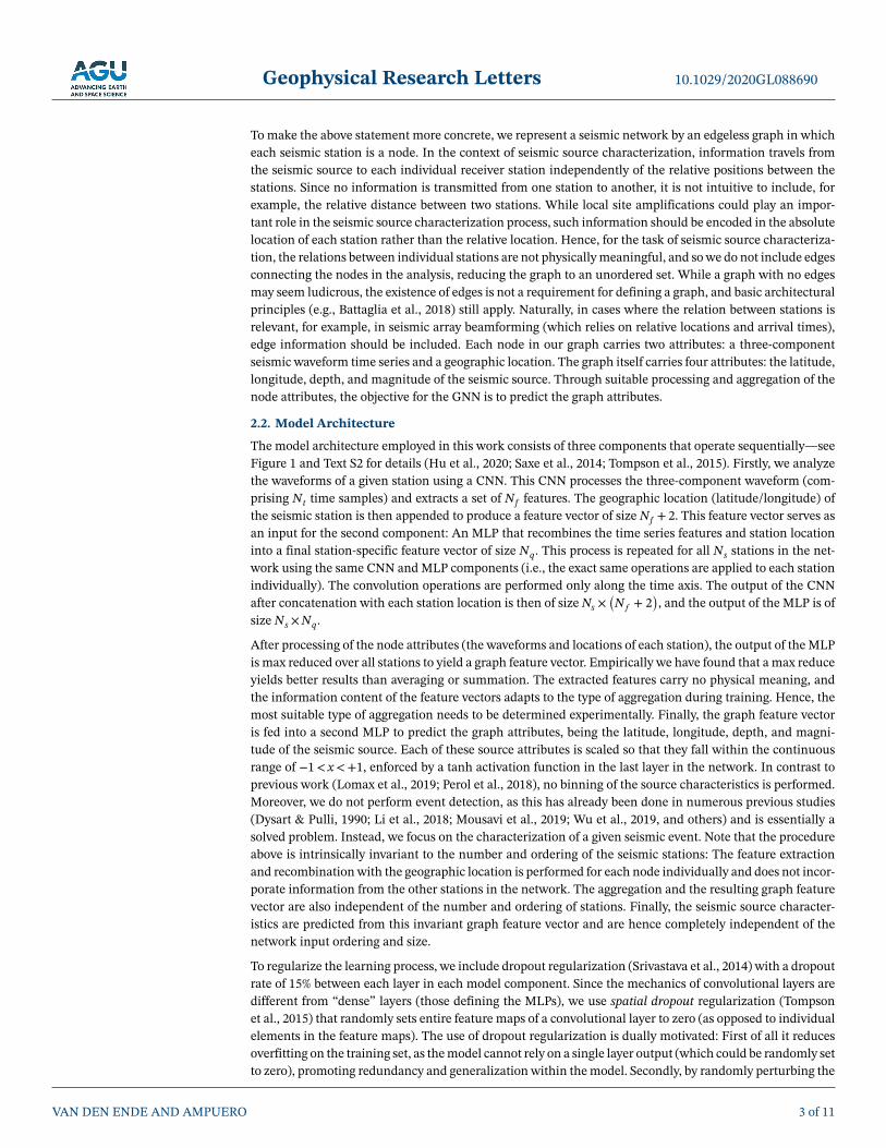
To make the above statement more concrete, we represent a seismic network by an edgeless graph in whicheach seismic station is a node. In the context of seismic source characterization, information travels fromthe seismic source to each individual receiver station independently of the relative positions between thestations. Since no information is transmitted from one station to another, it is not intuitive to include, forexample, the relative distance between two stations. While local site amplifications could play an impor-tant role in the seismic source characterization process, such information should be encoded in the absolutelocation of each station rather than the relative location. Hence, for the task of seismic source characteriza-tion, the relations between individual stations are not physically meaningful, and so we do not include edgesconnecting the nodes in the analysis, reducing the graph to an unordered set. While a graph with no edgesmay seem ludicrous, the existence of edges is not a requirement for defining a graph, and basic architecturalprinciples (e.g., Battaglia et al., 2018) still apply. Naturally, in cases where the relation between stations isrelevant, for example, in seismic array beamforming (which relies on relative locations and arrival times),edge information should be included. Each node in our graph carries two attributes: a three-componentseismic waveform time series and a geographic location. The graph itself carries four attributes: the latitude,longitude, depth, and magnitude of the seismic source. Through suitable processing and aggregation of thenode attributes, the objective for the GNN is to predict the graph attributes.

2.2. Model Architecture

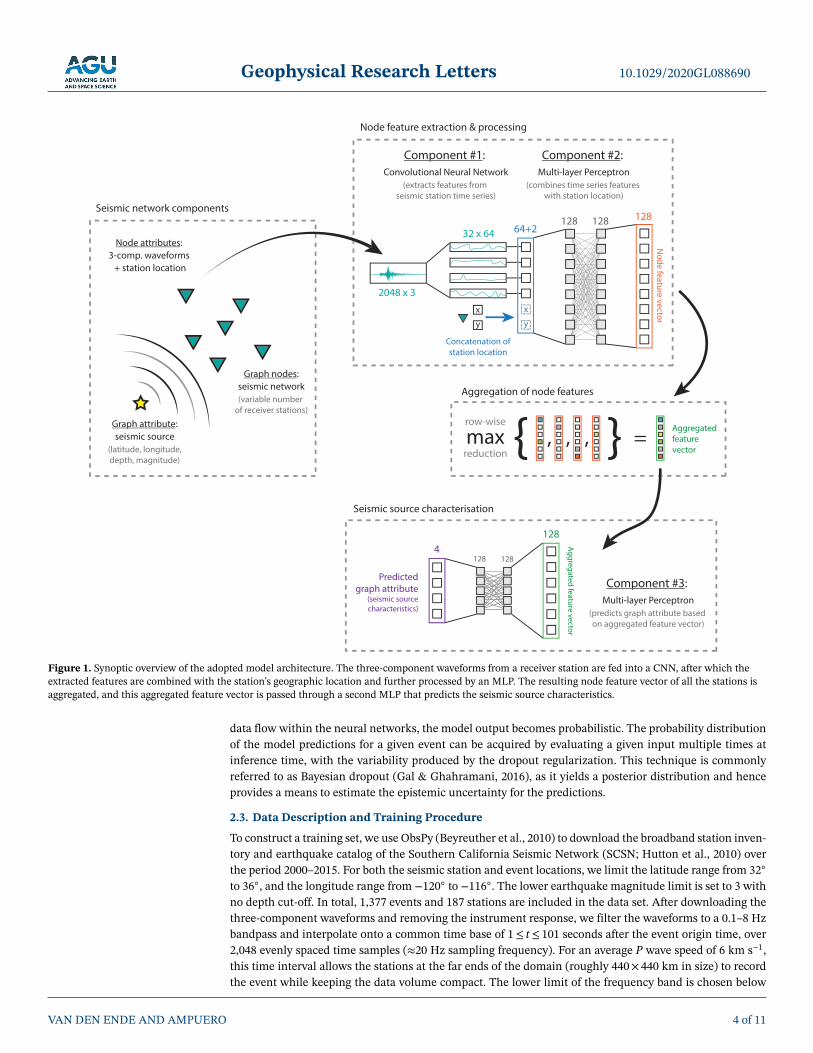
The model architecture employed in this work consists of three components that operate sequentially—seeFigure 1 and Text S2 for details (Hu et al., 2020; Saxe et al., 2014; Tompson et al., 2015). Firstly, we analyzethe waveforms of a given station using a CNN. This CNN processes the three-component waveform (com-prising Nt time samples) and extracts a set of Nf features. The geographic location (latitude/longitude) ofthe seismic station is then appended to produce a feature vector of size Nf + 2. This feature vector serves asan input for the second component: An MLP that recombines the time series features and station locationinto a final station-specific feature vector of size Nq. This process is repeated for all Ns stations in the net-work using the same CNN and MLP components (i.e., the exact same operations are applied to each stationindividually). The convolution operations are performed only along the time axis. The output of the CNNafter concatenation with each station location is then of size Ns ×

(N𝑓 + 2

), and the output of the MLP is of

size Ns ×Nq.

After processing of the node attributes (the waveforms and locations of each station), the output of the MLPis max reduced over all stations to yield a graph feature vector. Empirically we have found that a max reduceyields better results than averaging or summation. The extracted features carry no physical meaning, andthe information content of the feature vectors adapts to the type of aggregation during training. Hence, themost suitable type of aggregation needs to be determined experimentally. Finally, the graph feature vectoris fed into a second MLP to predict the graph attributes, being the latitude, longitude, depth, and magni-tude of the seismic source. Each of these source attributes is scaled so that they fall within the continuousrange of −1< x <+1, enforced by a tanh activation function in the last layer in the network. In contrast toprevious work (Lomax et al., 2019; Perol et al., 2018), no binning of the source characteristics is performed.Moreover, we do not perform event detection, as this has already been done in numerous previous studies(Dysart & Pulli, 1990; Li et al., 2018; Mousavi et al., 2019; Wu et al., 2019, and others) and is essentially asolved problem. Instead, we focus on the characterization of a given seismic event. Note that the procedureabove is intrinsically invariant to the number and ordering of the seismic stations: The feature extractionand recombination with the geographic location is performed for each node individually and does not incor-porate information from the other stations in the network. The aggregation and the resulting graph featurevector are also independent of the number and ordering of stations. Finally, the seismic source character-istics are predicted from this invariant graph feature vector and are hence completely independent of thenetwork input ordering and size.

To regularize the learning process, we include dropout regularization (Srivastava et al., 2014) with a dropoutrate of 15% between each layer in each model component. Since the mechanics of convolutional layers aredifferent from “dense” layers (those defining the MLPs), we use spatial dropout regularization (Tompsonet al., 2015) that randomly sets entire feature maps of a convolutional layer to zero (as opposed to individualelements in the feature maps). The use of dropout regularization is dually motivated: First of all it reducesoverfitting on the training set, as the model cannot rely on a single layer output (which could be randomly setto zero), promoting redundancy and generalization within the model. Secondly, by randomly perturbing the

VAN DEN ENDE AND AMPUERO 3 of 11

Geophysical Research Letters 10.1029/2020GL088690

Figure 1. Synoptic overview of the adopted model architecture. The three-component waveforms from a receiver station are fed into a CNN, after which theextracted features are combined with the station's geographic location and further processed by an MLP. The resulting node feature vector of all the stations isaggregated, and this aggregated feature vector is passed through a second MLP that predicts the seismic source characteristics.

data flow within the neural networks, the model output becomes probabilistic. The probability distributionof the model predictions for a given event can be acquired by evaluating a given input multiple times atinference time, with the variability produced by the dropout regularization. This technique is commonlyreferred to as Bayesian dropout (Gal & Ghahramani, 2016), as it yields a posterior distribution and henceprovides a means to estimate the epistemic uncertainty for the predictions.

2.3. Data Description and Training Procedure

To construct a training set, we use ObsPy (Beyreuther et al., 2010) to download the broadband station inven-tory and earthquake catalog of the Southern California Seismic Network (SCSN; Hutton et al., 2010) overthe period 2000–2015. For both the seismic station and event locations, we limit the latitude range from 32◦

to 36◦, and the longitude range from −120◦ to −116◦. The lower earthquake magnitude limit is set to 3 withno depth cut-off. In total, 1,377 events and 187 stations are included in the data set. After downloading thethree-component waveforms and removing the instrument response, we filter the waveforms to a 0.1–8 Hzbandpass and interpolate onto a common time base of 1≤ t ≤ 101 seconds after the event origin time, over2,048 evenly spaced time samples (≈20 Hz sampling frequency). For an average P wave speed of 6 km s−1,this time interval allows the stations at the far ends of the domain (roughly 440× 440 km in size) to recordthe event while keeping the data volume compact. The lower limit of the frequency band is chosen below

VAN DEN ENDE AND AMPUERO 4 of 11

Geophysical Research Letters 10.1029/2020GL088690

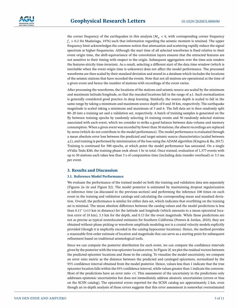
the corner frequency of the earthquakes in this analysis (Mw < 6, with corresponding corner frequencyf c > 0.2 Hz Madariaga, 1976) such that information regarding the seismic moment is retained. The upperfrequency limit acknowledges the common notion that attenuation and scattering rapidly reduce the signalspectrum at higher frequencies. Although the start time of all selected waveforms is fixed relative to theirevent origin time, the shift-equivariance of the convolution layers ensures that the extracted features arenot sensitive to their timing with respect to the origin. Subsequent aggregation over the time-axis rendersthe features strictly time-invariant. As a result, selecting a different start of the data time window (which isinevitable when the event origin time is unknown) does not affect the model performance. The processedwaveforms are then scaled by their standard deviation and stored in a database which includes the locationsof the seismic stations that have recorded the events. Note that not all stations are operational at the time ofa given event and hence the number of stations with recordings of the event varies.

After processing the waveforms, the locations of the stations and seismic source are scaled by the minimumand maximum latitude/longitude, so that the rescaled locations fall in the range of ±1. Such normalizationis generally considered good practice in deep learning. Similarly, the source depth is scaled to fall in thesame range by taking a minimum and maximum source depth of 0 and 30 km, respectively. The earthquakemagnitude is scaled taking a minimum and maximum of 3 and 6. The full data set is then randomly split80–20 into a training set and a validation set, respectively. A batch of training samples is generated on thefly between training epochs by randomly selecting 16 training events and 50 randomly selected stationsassociated with each event, which we consider to strike a good balance between data volume and memoryconsumption. When a given event was recorded by fewer than 50 stations, the absent recordings are replacedby zeros (which do not contribute to the model performance). The model performance is evaluated througha mean absolute error loss between the predicted and target seismic source characteristics (scaled between±1), and training is performed by minimization of the loss using the ADAM algorithm (Kingma & Ba, 2017).Training is continued for 500 epochs, at which point the model performance has saturated. On a singlenVidia Tesla K80, the training phase took about 1 hr in total. Once trained, evaluation of 1,377 events withup to 50 stations each takes less than 5 s of computation time (including data transfer overhead) or 3.5 msper event.

3. Results and Discussion3.1. Reference Model Performance

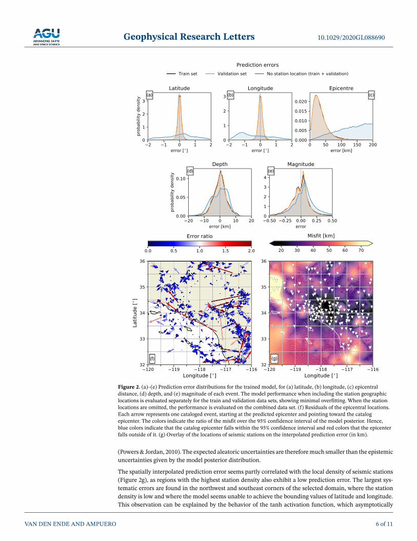
We evaluate the performance of the trained model on both the training and validation data sets separately(Figures 2a–2e and Figure S2). The model posterior is estimated by maintaining dropout regularizationat inference time (as discussed in the previous section) and performing the inference 100 times on eachevent in the training and validation catalogs and calculating the corresponding mean and standard devia-tion. Overall, the performance is similar for either data set, which indicates that overfitting on the trainingset is minimal. The mean absolute difference between the catalog values and the model predictions is lessthan 0.11◦ (≈13 km in distance) for the latitude and longitude (which amounts to a mean epicentral loca-tion error of 18 km), 3.3 km for the depth, and 0.13 for the event magnitude. While these predictions arenot as precise as typical nonrelocated estimates for Southern California (Powers & Jordan, 2010), they areobtained without phase picking or waveform amplitude modeling nor is a crustal velocity models explicitlyprovided (though it is implicitly encoded in the catalog hypocenter locations). Hence, the method providesa reasonable first-order estimate of location and magnitude that can serve as a starting point for subsequentrefinement based on traditional seismological tools.

Since we can compute the posterior distribution for each event, we can compare the confidence intervalsgiven by the posterior with the true epicenter location error. In Figure 2f, we plot the residual vectors betweenthe predicted epicenter locations and those in the catalog. To visualize the model uncertainty, we computean error ratio metric as the distance between the predicted and cataloged epicenters, normalized by the95% confidence interval obtained from the model posterior. Hence, values less than 1 indicate that the trueepicenter location falls within the 95% confidence interval, while values greater than 1 indicate the converse.Most of the predictions have an error ratio <1. This assessment of the uncertainty in the predictions onlyaddresses epistemic uncertainties but does not immediately address aleatoric uncertainties (errors or biason the SCSN catalog). The epicentral errors reported for the SCSN catalog are approximately 2 km, eventhough an in-depth analysis of these errors suggests that this error assessment is somewhat overestimated

VAN DEN ENDE AND AMPUERO 5 of 11

Geophysical Research Letters 10.1029/2020GL088690

Figure 2. (a)–(e) Prediction error distributions for the trained model, for (a) latitude, (b) longitude, (c) epicentraldistance, (d) depth, and (e) magnitude of each event. The model performance when including the station geographiclocations is evaluated separately for the train and validation data sets, showing minimal overfitting. When the stationlocations are omitted, the performance is evaluated on the combined data set. (f) Residuals of the epicentral locations.Each arrow represents one cataloged event, starting at the predicted epicenter and pointing toward the catalogepicenter. The colors indicate the ratio of the misfit over the 95% confidence interval of the model posterior. Hence,blue colors indicate that the catalog epicenter falls within the 95% confidence interval and red colors that the epicenterfalls outside of it. (g) Overlay of the locations of seismic stations on the interpolated prediction error (in km).

(Powers & Jordan, 2010). The expected aleatoric uncertainties are therefore much smaller than the epistemicuncertainties given by the model posterior distribution.

The spatially interpolated prediction error seems partly correlated with the local density of seismic stations(Figure 2g), as regions with the highest station density also exhibit a low prediction error. The largest sys-tematic errors are found in the northwest and southeast corners of the selected domain, where the stationdensity is low and where the model seems unable to achieve the bounding values of latitude and longitude.This observation can be explained by the behavior of the tanh activation function, which asymptotically

VAN DEN ENDE AND AMPUERO 6 of 11

Geophysical Research Letters 10.1029/2020GL088690

approaches its range of ±1, corresponding with the range of latitudes and longitudes of the training sam-ples. Hence, increasingly larger activations are required to push the final location predictions toward theboundaries of the domain, biasing the results toward the interior. This highlights a fundamental trade-offbetween resolution (prediction accuracy) in the interior of the data domain, and the maximum amplitudeof the predictions (which also applies to linear activation functions).

Lastly, we perform additional analyses of the sensitivity of the predictions to the signal-to-noise ratio, wave-form preprocessing, and epicenter location (Figures S4–S6). These analyses show that the predictions arerather robust to the event magnitude (as a first-order proxy for signal-to-noise ratio) and insensitive to instru-ment corrections. Moreover, preliminary tests, in which we adopted a filter passband of 0.5–5 Hz, indicatedthat the choice for the prefiltering frequency band had little influence on the model performance. When themodel is provided with waveforms belonging to an event with an epicenter outside of the selected trainingdomain, the model predictions for the epicenter location collapse to an average value around the center ofthe domain (Figure S6). Fortunately, the uncertainty of the predictions (inferred from the posterior distri-bution of each event) is also much larger than for events that are located within the domain. Thus, exteriorevents can be distinguished from interior events through the inferred precision.

3.2. Influence of Geographic Information on Location Accuracy

A direct test to assess whether the station geographic location information is actually used in making thepredictions (and therefore holds predictive value), we perform inference on the full data set but set the sta-tion coordinates to a fixed mean value of (34◦, −118◦)—see Figures 2a–2e and S3. While the predictions forthe event magnitude remain mostly unchanged, the estimation of the epicenter location deteriorates andbecomes broadly distributed (typical for random predictions). This clearly indicates that the station locationinformation plays an important role in estimating the epicenter locations. Thus, the adopted GNN approach,in which station location information is provided explicitly, holds an advantage over station-location agnos-tic methods. Interestingly, the event magnitude is almost as well resolved as when the station coordinatesare included, which suggests that the model relies on the waveform data but not on station locations toestimate the magnitude. This was also observed by Mousavi and Beroza (2020b), who proposed that therelative timing of the P and S wave arrivals may encode epicentral distance information. Combined withthe amplitude of the waveforms, this may implicitly encode magnitude information. Additional analysis ofthe contributions of (parts of) the waveforms and station locations to each of the prediction components(e.g., using Grad-CAM; Selvaraju et al., 2019) will shed more light on this.

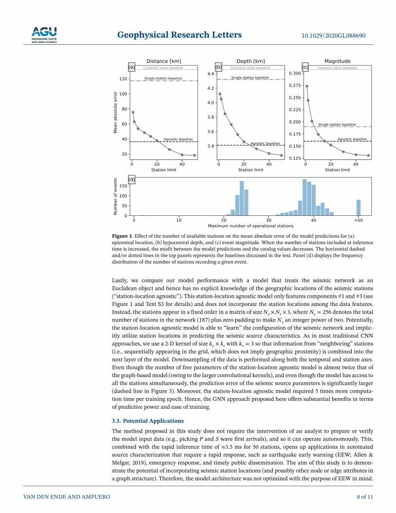
Related to this, we investigate the effect of the (maximum) number of stations included at inference timeby selecting, for each event, the stations recording the waveforms with the M highest standard deviations.All other waveforms are set to zero and therefore do not contribute to the predictions. If a given event wasrecorded by fewer than M stations, only the maximum number of operational stations was used with noaugmentation. We perform the inference for M = {1, 2, 5, 10, 15, 20, 30, 40, 50} stations and compute themean absolute error of the predictions for the epicenter location (expressed as a distance in km; Figure 3a),hypocentral depth (Figure 3b), and event magnitude (Figure 3c). For all the predicted quantities, we observethat the misfit with the catalog values rapidly decreases with the maximum number of stations includedin the analysis, until the performance saturates at around M ≥ 40. The reason for this saturation may lie inthe distribution of the number of operational stations per event (Figure 3d). Since the majority of catalogedevents is recorded by fewer than 40 stations, increasing M beyond 40 is only potentially beneficial only fora small number of events. For reference, we compute two performance baselines: Firstly, we take the meanvalue of each quantity (latitude, longitude, depth, and magnitude) over the catalog and calculate the meanabsolute error relative to these. This baseline represents the performance of a “biased coin flip” (i.e., randomguessing). Secondly, we train our model specifically using only a single station per training sample, throughwhich the method specializes to single-waveform analysis (c.f. Lomax et al., 2019; Mousavi & Beroza, 2020b;Perol et al., 2018). These baselines are included in Figure 3 as horizontal dotted and dashed-dotted lines forthe mean absolute error relative to the (constant value) mean and for the single-station model, respectively.Strikingly, the model that was trained on the single-station waveforms achieves worse performance in termsof the predicted hypocenter locations than the model trained on 50 stations but using only a single station atinference time. A possible explanation for this is that the single-station model may have gotten attracted to apoor local minimum in the loss landscape, after which the model started overfitting, whereas the 50-stationmodel was able to generalize better and descended into a better local minimum.

VAN DEN ENDE AND AMPUERO 7 of 11

Geophysical Research Letters 10.1029/2020GL088690

Figure 3. Effect of the number of available stations on the mean absolute error of the model predictions for (a)epicentral location, (b) hypocentral depth, and (c) event magnitude. When the number of stations included at inferencetime is increased, the misfit between the model predictions and the catalog values decreases. The horizontal dashedand/or dotted lines in the top panels represents the baselines discussed in the text. Panel (d) displays the frequencydistribution of the number of stations recording a given event.

Lastly, we compare our model performance with a model that treats the seismic network as anEuclidean object and hence has no explicit knowledge of the geographic locations of the seismic stations(“station-location agnostic”). This station-location agnostic model only features components #1 and #3 (seeFigure 1 and Text S3 for details) and does not incorporate the station locations among the data features.Instead, the stations appear in a fixed order in a matrix of size Ns ×Nt × 3, where Ns = 256 denotes the totalnumber of stations in the network (187) plus zero padding to make Ns an integer power of two. Potentially,the station-location agnostic model is able to “learn” the configuration of the seismic network and implic-itly utilize station locations in predicting the seismic source characteristics. As in most traditional CNNapproaches, we use a 2-D kernel of size ks × kt with ks = 3 so that information from “neighboring” stations(i.e., sequentially appearing in the grid, which does not imply geographic proximity) is combined into thenext layer of the model. Downsampling of the data is performed along both the temporal and station axes.Even though the number of free parameters of the station-location agnostic model is almost twice that ofthe graph-based model (owing to the larger convolutional kernels), and even though the model has access toall the stations simultaneously, the prediction error of the seismic source parameters is significantly larger(dashed line in Figure 3). Moreover, the station-location agnostic model required 5 times more computa-tion time per training epoch. Hence, the GNN approach proposed here offers substantial benefits in termsof predictive power and ease of training.

3.3. Potential Applications

The method proposed in this study does not require the intervention of an analyst to prepare or verifythe model input data (e.g., picking P and S wave first arrivals), and so it can operate autonomously. This,combined with the rapid inference time of ≈3.5 ms for 50 stations, opens up applications in automatedsource characterization that require a rapid response, such as earthquake early warning (EEW; Allen &Melgar, 2019), emergency response, and timely public dissemination. The aim of this study is to demon-strate the potential of incorporating seismic station locations (and possibly other node or edge attributes ina graph structure). Therefore, the model architecture was not optimized with the purpose of EEW in mind.

VAN DEN ENDE AND AMPUERO 8 of 11

Geophysical Research Letters 10.1029/2020GL088690

Nonetheless, its modular nature allows for modifications required to accommodate the real-time demandsof EEW.

The first out of three components of this model consists of a CNN that analyses the waveforms of eachseismic station and yields a set of station-specific features. The advantage of using a CNN is that it hasimmediate access to all the available information to produce a set of features optimal for the subsequentMLP components. Alternatively, a different class of deep neural networks suitable for time series analysis,the recurrent neural networks (RNN; Hochreiter & Schmidhuber, 1997; Sherstinsky, 2020), allows for online(real-time) processing of time series. Within the generalized framework of GNNs (Battaglia et al., 2018),replacing the first CNN component with an RNN produces an equally valid model architecture, althoughtraining and interpreting RNNs comes with new challenges compared with conventional CNNs. At inferencetime, for each new data entry the output of the first GNN component is updated for each station individually,which could be aggregated periodically to update the final model predictions, taking into account previouslyseen data (the “memory” of the RNN). A robust prediction will be one for which the output of the modelconverges to a stable estimate of hypocenter location and magnitude. Since we here employed a CNN ratherthan an RNN, we do not know how much time since the first ground motions is required to converge toa stable prediction, and we anticipate that this convergence depends on the quality and consistency of thedata. Moreover, different components of the prediction may converge at different rates: While the hypocenterestimate may be governed by the (first) arrival of seismic energy at the various stations in the region (andtherefore on the station density), the magnitude estimate is potentially controlled by the duration of themoment-rate function (Meier et al., 2017). Owing to the opacity of our deep learning method, we cannotdirectly assess which part of the input governs which part in the output, and so this will need to be assessedempirically.

As mentioned in section 2.2, we focused our efforts on seismic source characterization and not event detec-tion. For any EEW task, earthquake detection is a crucial first step, which fortunately has been demonstratedto be a task suitable for machine learning methods (e.g., Dysart & Pulli, 1990; Li et al., 2018; Mousaviet al., 2019; Wu et al., 2019). In the methods proposed in the present study, earthquake detection could beperformed by adding an additional graph attribute (alongside latitude, longitude, depth, and magnitude)indicating whether or not an event has been detected (similar to Lomax et al., 2019; Perol et al., 2018). Alter-natively, a dedicated detection algorithm (based on machine learning or otherwise) could run in paralleland trigger the source characterization algorithm once an event has been detected. This second approachsignificantly reduces computational overhead. Flexibility in the number of stations included in the modelinput facilitates processing of an expanding data set as more seismic stations experience ground shakingafter the first detection.

For the applications of emergency response and information dissemination, the real-time requirements areless stringent, so that some response time may be sacrificed in favor of prediction accuracy, maintainingthe CNN component #1. Our method can be readily applied to automated earthquake catalog generation inregions where large volumes of raw data exist but which have not been fully processed. This typically arisesin aftershock campaigns with stations that were not telemetered, for instance Ocean Bottom Seismometers.Given the relatively small size of the GNN employed here, retraining a pretrained model on data from a dif-ferent region is relatively inexpensive. Out of the 110,836 trainable parameters, less than half (42,244) residein the second and third components of the network. The first CNN component is completely agnostic to anyspatial or regional information, as it only extracts features from time series of individual stations. Hence,if the waveforms in the target region are similar to those in the initial training region, the first componentrequires no retraining. This leaves only the smaller second and third MLP components to be retrained andadapted to the characteristics of the target region. As such, fewer training seismic events than employed forthe initial training will be required for fine-tuning of the model. It is crucial to realize here that the secondand third components potentially encode the crustal velocity structure and local site amplifications and aretherefore specific to the domain that was selected during training (Southern California). Direct applicationof the trained model to other regions without retraining is unwarranted. The scaling of the retrained modelperformance with the number of stations will need to be assessed empirically, as it may be sensitive to stationredundancy, and spatial coverage and density.

VAN DEN ENDE AND AMPUERO 9 of 11

Geophysical Research Letters 10.1029/2020GL088690

Aside from automatically providing an earthquake catalog, the estimates of the seismic source locationscan offer a suitable starting point for additional seismological analyses. With the retrained model, the pre-dicted hypocenter locations yield approximate phase arrival times at the various stations in the seismicnetwork, which serve as a basis to set the windows for cross-correlation time-delay estimation and subse-quent double-difference relocation. Grid-search based inversion efforts could be directed to a region aroundthe predicted hypocenter location, rather than expanding the search of candidate source locations to a muchlarger (regional) domain. Even though the model predictions for the epicentral locations are larger thanwhat conventional seismological techniques can achieve, there is merit in deep learning based automatedsource characterization to expedite current seismological workflows.

Lastly, we point out that the GNN approach is rather general and that it may be adopted in other applicationssuch as seismic event detection or classification that benefit from geographic or relational information ofthe seismic network. Aside from predicting “global” graph attributes, like was done in this study, GNNs canalso be employed to predict node or edge attributes. Examples of such attributes include site amplificationfactors and event detections for the nodes (seismic stations) and phase associations for the edges. Sincemany geophysical data are inherently non-Euclidean, graph-based approaches offer a natural choice for theanalysis of these data and permit creative solutions to present-day challenges.

4. ConclusionsIn this study we propose a method to incorporate the geometry of a seismic network into deep learningarchitectures using a graph neural network (GNN) approach, applied to the task of seismic source char-acterization (earthquake location and magnitude estimation). By incorporating the geographic location ofstations into the learning and prediction process, we find that the deep learning model achieves superior per-formance in predicting the seismic source characteristics (epicentral latitude/longitude, hypocentral depth,and event magnitude) compared to a model that is agnostic to the layout of the seismic network. In this way,multistation waveforms can be incorporated while preserving flexibility to the number of available seismicstations, and invariance to the ordering of the station recordings. The GNN-based approach warrants theexploration of new avenues in earthquake early warning and rapid earthquake information dissemination,as well as in automated earthquake catalog generation or other seismological tasks.

Data Availability StatementPython codes and the pretrained model are available online (https://doi.org/10.6084/m9.figshare.12231077).

ReferencesAllen, R. M., & Melgar, D. (2019). Earthquake early warning: Advances, scientific challenges, and societal needs. Annual Review of Earth

and Planetary Sciences, 47(1), 361–388. https://doi.org/10.1146/annurev-earth-053018-060457Battaglia, P. W., Hamrick, J. B., Bapst, V., Sanchez-Gonzalez, A., Zambaldi, V., Malinowski, M., & Pascanu, R. (2018). Relational inductive

biases, deep learning, and graph networks. arXiv:1806.01261 [cs, stat].Beyreuther, M., Barsch, R., Krischer, L., Megies, T., Behr, Y., & Wassermann, J. (2010). ObsPy: A Python toolbox for seismology.

Seismological Research Letters, 81(3), 530–533. https://doi.org/10.1785/gssrl.81.3.530Bronstein, M. M., Bruna, J., LeCun, Y., Szlam, A., & Vandergheynst, P. (2017). Geometric deep learning: Going beyond Euclidean data.

IEEE Signal Processing Magazine, 34(4), 18–42. https://doi.org/10.1109/MSP.2017.2693418Cui, Z., Henrickson, K., Ke, R., & Wang, Y. (2019). Traffic graph convolutional recurrent neural network: A deep learning framework for

network-scale traffic learning and forecasting. In IEEE Transactions on Intelligent Transportation Systems (pp. 1–2). IEEE. https://doi.org/10.1109/TITS.2019.2950416

Duvenaud, D. K., Maclaurin, D., Iparraguirre, J., Bombarell, R., Hirzel, T., Aspuru-Guzik, A., & Adams, R. P. (2015). Convolutionalnetworks on graphs for learning molecular fingerprints. In C. Cortes, N. D. Lawrence, D. D. Lee, M. Sugiyama, & R. Garnett (Eds.),Advances in neural information processing systems (Vol. 28, pp. 2224–2232). Red Hook, NY: Curran Associates, Inc.

Dysart, P. S., & Pulli, J. J. (1990). Regional seismic event classification at the NORESS array: Seismological measurements and the use oftrained neural networks. Bulletin of the Seismological Society of America, 80(6B), 1910–1933.

Fukushima, K. (1980). Neocognitron: A self-organizing neural network model for a mechanism of pattern recognition unaffected by shiftin position. Biological Cybernetics, 36(4), 193–202. https://doi.org/10.1007/BF00344251

Gal, Y., & Ghahramani, Z. (2016). Dropout as a Bayesian approximation: Representing model uncertainty in deep learning. Proceedings ofthe 33rd International Conference on International Conference on Machine Learning, 48, 1050–1059.

Gilmer, J., Schoenholz, S. S., Riley, P. F., Vinyals, O., & Dahl, G. E. (2017). Neural message passing for quantum chemistry. Proceedings ofthe 34th International Conference on Machine Learning, 70, 1263–1272.

Gori, M., Monfardini, G., & Scarselli, F. (2005). A new model for learning in graph domains, Proceedings 2005 IEEE International JointConference on Neural Networks (Vol. 2, pp. 729–734). Montreal, Quebec, CA: IEEE. https://doi.org/10.1109/IJCNN.2005.1555942

Hamilton, W. L., Ying, R., & Leskovec, J. (2017). Inductive representation learning on large graphs. In Proceedings of the 31st InternationalConference on Neural Information Processing Systems (pp. 1025–1035). Long Beach, California, USA: Curran Associates Inc.

AcknowledgmentsWe thank the Associate Editor and twoanonymous reviewers for theirthoughtful comments on themanuscript. MvdE is supported byFrench government through theUCAJEDI Investments in the Futureproject managed by the NationalResearch Agency (ANR) with thereference number ANR-15-IDEX-01.The authors acknowledgecomputational resources provided bythe ANR JCJC E-POST project(ANR-14-CE03-0002-01JCJC E-POST).

VAN DEN ENDE AND AMPUERO 10 of 11

Geophysical Research Letters 10.1029/2020GL088690

Hochreiter, S., & Schmidhuber, J. (1997). Long short-term memory. Neural Computation, 9(8), 1735–1780. https://doi.org/10.1162/neco.1997.9.8.1735

Hu, W., Xiao, L., & Pennington, J. (2020). Provable benefit of orthogonal initialization in optimizing deep linear networks.arXiv:2001.05992 [cs, math, stat].

Hutton, K., Woessner, J., & Hauksson, E. (2010). Earthquake monitoring in southern California for seventy-seven years (1932–2008).Bulletin of the Seismological Society of America, 100(2), 423–446. https://doi.org/10.1785/0120090130

Käufl, P., Valentine, A. P., O'Toole, T. B., & Trampert, J. (2014). A framework for fast probabilistic centroid-moment-tensordetermination—Inversion of regional static displacement measurements. Geophysical Journal International, 196(3), 1676–1693.https://doi.org/10.1093/gji/ggt473

Kingma, D. P., & Ba, J. (2017). Adam: A method for stochastic optimization. arXiv:1412.6980 [cs].Kriegerowski, M., Petersen, G. M., Vasyura-Bathke, H., & Ohrnberger, M. (2019). A deep convolutional neural network for localization of

clustered earthquakes based on multistation full waveforms. Seismological Research Letters, 90(2A), 510–516. https://doi.org/10.1785/0220180320

LeCun, Y., Bengio, Y., & Hinton, G. (2015). Deep learning. Nature, 521(7553), 436–444. https://doi.org/10.1038/nature14539Li, Z., Meier, M. A., Hauksson, E., Zhan, Z., & Andrews, J. (2018). Machine learning seismic wave discrimination: Application to

earthquake early warning. Geophysical Research Letters, 45, 4773–4779. https://doi.org/10.1029/2018GL077870Lomax, A., Michelini, A., & Jozinovic, D. (2019). An investigation of rapid earthquake characterization using single station waveforms

and a convolutional neural network. Seismological Research Letters, 90(2A), 517–529. https://doi.org/10.1785/0220180311Madariaga, R. (1976). Dynamics of an expanding circular fault. Bulletin of the Seismological Society of America, 66, 639–666.Meier, M. A., Ampuero, J. P., & Heaton, T. H. (2017). The hidden simplicity of subduction megathrust earthquakes. Science, 357(6357),

1277–1281. https://doi.org/10.1126/science.aan5643Monti, F., Boscaini, D., Masci, J., Rodolà, E., Svoboda, J., & Bronstein, M. M. (2017). Geometric deep learning on graphs and manifolds

using mixture model cnns. In 2017 IEEE Conference on Computer Vision and Pattern Recognition (CVPR) (pp. 5425–5434). https://doi.org/10.1109/CVPR.2017.576

Mousavi, S. M., & Beroza, G. C. (2020a). Bayesian-deep-learning estimation of earthquake location from single-station observations. InIEEE Transactions on Geoscience and Remote Sensing (pp. 1–14). https://doi.org/10.1109/TGRS.2020.2988770

Mousavi, S. M., & Beroza, G. C. (2020b). A machine-learning approach for earthquake magnitude estimation. Geophysical ResearchLetters, 47, e2019GL085976. https://doi.org/10.1029/2019GL085976

Mousavi, S. M., Zhu, W., Sheng, Y., & Beroza, G. C. (2019). CRED: A deep residual network of convolutional and recurrent units forearthquake signal detection. Scientific Reports, 9(1), 1–14. https://doi.org/10.1038/s41598-019-45748-1

Perol, T., Gharbi, M., & Denolle, M. (2018). Convolutional neural network for earthquake detection and location. Science Advances, 4(2),e1700578. https://doi.org/10.1126/sciadv.1700578

Powers, P. M., & Jordan, T. H. (2010). Distribution of seismicity across strike-slip faults in California. Journal of Geophysical Research,115, B05305. https://doi.org/10.1029/2008JB006234

Qi, C. R., Yi, L., Su, H., & Guibas, L. J. (2017). Pointnet++: Deep hierarchical feature learning on point sets in a metric space. InProceedings of the 31st International Conference on Neural Information Processing Systems (pp. 5105–5114). Long Beach, California,USA: Curran Associates Inc.

Rosenblatt, F. (1957). The perceptron: A perceiving and recognizing automaton (Tech. Rep. No. 85-60-1). Buffalo, New York: CornellAeronautical Laboratory.

Rumelhart, D. E., Hinton, G. E., & Williams, R. J. (1986). Learning representations by back-propagating errors. Nature, 323(6088),533–536. https://doi.org/10.1038/323533a0

Sanchez-Gonzalez, A., Bapst, V., Cranmer, K., & Battaglia, P. (2019). Hamiltonian graph networks with ode integrators. arXiv:1909.12790[physics].

Saxe, A., McClelland, J. L., & Ganguli, S. (2014). Exact solutions to the nonlinear dynamics of learning in deep linear neural networks. InInternational Conference on Learning Representations.

Scarselli, F., Gori, M., Tsoi, A. C., Hagenbuchner, M., & Monfardini, G. (2009). The graph neural network model. IEEE Transactions onNeural Networks, 20(1), 61–80. https://doi.org/10.1109/TNN.2008.2005605

Schramowski, P., Stammer, W., Teso, S., Brugger, A., Luigs, H. G., Mahlein, A. K., & Kersting, K. (2020). Right for the wrong scientificreasons: Revising deep networks by interacting with their explanations. arXiv:2001.05371 [cs, stat].

Selvaraju, R. R., Cogswell, M., Das, A., Vedantam, R., Parikh, D., & Batra, D. (2019). Grad-cam: Visual explanations from deep networksvia gradient-based localization. International Journal of Computer Vision, 128, 336–359. https://doi.org/10.1007/s11263-019-01228-7

Sherstinsky, A. (2020). Fundamentals of recurrent neural network (RNN) and long short-term memory (LSTM) network. Physica D:Nonlinear Phenomena, 404, 132306. https://doi.org/10.1016/j.physd.2019.132306

Srivastava, N., Hinton, G., Krizhevsky, A., Sutskever, I., & Salakhutdinov, R. (2014). Dropout: A simple way to prevent neural networksfrom overfitting. Journal of Machine Learning Research, 15(56), 1929–1958.

Tompson, J., Goroshin, R., Jain, A., LeCun, Y., & Bregler, C. (2015). Efficient object localization using convolutional networks. In 2015IEEE Conference on Computer Vision and Pattern Recognition (CVPR) (pp. 648–656). https://doi.org/10.1109/CVPR.2015.7298664

Wang, Y., Sun, Y., Liu, Z., Sarma, S. E., Bronstein, M. M., & Solomon, J. M. (2019). Dynamic graph cnn for learning on point clouds.Association for Computing Machinery.

Wu, Y., Lin, Y., Zhou, Z., Bolton, D. C., Liu, J., & Johnson, P. (2019). DeepDetect: A cascaded region-based densely connected network forseismic event detection. IEEE Transactions on Geoscience and Remote Sensing, 57(1), 62–75. https://doi.org/10.1109/TGRS.2018.2852302

Zhou, J., Cui, G., Zhang, Z., Yang, C., Liu, Z., Wang, L., & Sun, M. (2019). Graph neural networks: A review of methods and applications.arXiv:1812.08434 [cs, stat].

VAN DEN ENDE AND AMPUERO 11 of 11