Automated Proof Checking in Introductory DiscreteMathematics Classes

by

Andrew J. Haven

S.B. Mathematics and Computer Science and EngineeringMassachusetts Institute of Technology, 2012

Submitted to the Department of Electrical Engineering and Computer Sciencein partial fulfillment of the requirements for the degree of

Master of Engineering in Electrical Engineering and Computer Science

at the

MASSACHUSETTS INSTITUTE OF TECHNOLOGY

June 2013

c© Massachusetts Institute of Technology 2013. All rights reserved.

Author . . . . . . . . . . . . . . . . . . . . . . . . . . . . . . . . . . . . . . . . . . . . . . . . . . . . . . . . . . . . . . . . . . . . . .Department of Electrical Engineering and Computer Science

May 24, 2013

Certified by. . . . . . . . . . . . . . . . . . . . . . . . . . . . . . . . . . . . . . . . . . . . . . . . . . . . . . . . . . . . . . . . . .Adam Chlipala, Assistant Professor, Thesis Supervisor

May 24, 2013

Accepted by . . . . . . . . . . . . . . . . . . . . . . . . . . . . . . . . . . . . . . . . . . . . . . . . . . . . . . . . . . . . . . . . .Prof. Dennis M. Freeman

Chairman, Masters of Engineering Thesis Committee

Automated Proof Checking in Introductory Discrete Mathematics

Classes

by

Andrew J. Haven

Submitted to the Department of Electrical Engineering and Computer Scienceon May 24, 2013, in partial fulfillment of the

requirements for the degree ofMaster of Engineering in Electrical Engineering and Computer Science

Abstract

Mathematical rigor is an essential concept to learn in the study of computer science. In theprocess of learning to write math proofs, instructors are heavily involved in giving feedbackabout correct and incorrect proofs. Computerized feedback in this area can ease the burdenon instructors and help students learn more efficiently. Several software packages exist thatcan verify proofs written in specific programming languages; these tools have support forsome basic topics that undergraduates learn, but not all. In this thesis, we develop librariesand proof automation for introductory combinatorics and probability concepts using Coq,an interactive theorem proving language.

Thesis Supervisor: Adam ChlipalaTitle: Assistant Professor

Acknowledgments

Many thanks to my advisor, Adam Chlipala, for suggesting this avenue of work and providingguidance and insight along the way. Thanks to my parents for their proofreading aid andconstant support. Thanks also to Jason Gross for helping with various Coq issues andsuggesting the function notation of Section 3.4.

6

Contents

1 Introduction 9

2 Previous Work 13

3 Combinatorics 15

3.1 Counting Example . . . . . . . . . . . . . . . . . . . . . . . . . . . . . . . . 15

3.2 Combinatorics Foundations . . . . . . . . . . . . . . . . . . . . . . . . . . . 19

3.2.1 Functions and Relations . . . . . . . . . . . . . . . . . . . . . . . . . 19

3.2.2 Cardinality . . . . . . . . . . . . . . . . . . . . . . . . . . . . . . . . 23

3.2.3 Finite Cardinalities . . . . . . . . . . . . . . . . . . . . . . . . . . . . 24

3.2.4 Product and Sum of Cardinalities . . . . . . . . . . . . . . . . . . . . 27

3.2.5 Cardinalities of Subsets . . . . . . . . . . . . . . . . . . . . . . . . . . 32

3.3 Automating Counting Proofs . . . . . . . . . . . . . . . . . . . . . . . . . . . 34

3.4 n-ary Function Notation . . . . . . . . . . . . . . . . . . . . . . . . . . . . . 46

4 Probability 51

4.1 Probability Example . . . . . . . . . . . . . . . . . . . . . . . . . . . . . . . 51

4.2 Probability Foundations . . . . . . . . . . . . . . . . . . . . . . . . . . . . . 53

5 Future Research 59

References 61

7

8

Chapter 1

Introduction

Students learning about computer science, as in other scientific disciplines, must learn to

articulate concepts rigorously and unambiguously. One begins to understand mathematical

rigor by writing detailed proofs that consider all possibilities. For students without an

extensive background in mathematics, this is a skill that needs to be gained concurrently to

learning the concepts of discrete mathematics that are pervasive in computer science. As a

beginner, mastering the writing of detailed proofs can be a difficult process. This requires a

healthy amount of feedback as to whether the proof steps used are correct and sufficiently

rigorous.

When writing code or learning similar engineering concepts, students often have auto-

matic feedback both from compilation or interpretation of their code and from running tests

written by instructors to test correctness of implementation. These kinds of feedback can

aid students in quickly correcting their mistakes during the problem-solving process without

having to wait for an instructor to grade or look at the work. In their mathematics classes,

students do not get to enjoy such rapid feedback because exercises involve writing down jus-

tified proofs which need to be hand-checked for correctness. We seek to gain the benefits of

computerized feedback in introductory undergraduate mathematics classes that teach proof

techniques through the use of automated theorem proving software. This project focuses on

concepts covered in MIT’s “Mathematics for Computer Science” class, otherwise known as

6.042, with material developed in [7]. While there are many topics covered in this discrete

math class, we focus specifically on combinatorics and probability.

9

To receive automated feedback about proof writing, students need to be able to write

proof steps in a programming langauge that can express these steps and verify their cor-

rectness. Automated and interactive theorem proving software are a class of programming

languages and tools used to write down and prove facts about mathematical and program

formalizations. These languages are used primarily by specialists to prove results that require

heavy amounts of casework and are intractable by hand. The first large-scale example of this

is the proof of the Four-Color Theorem [4], a proof which reduced down to 1, 936 machine-

checked cases. Each theorem prover uses a formal proof language to express definitions,

proofs, and results. A formal proof language contains a set of valid steps which can be used

to derive results from hypotheses in incremental steps. These steps are generally expressed

in terms that form the foundation of the language, similar to the axioms of Zermelo-Frenkel

set theory in mathematics, which can then be used to define other higher-level concepts.

Interactive theorem provers are provers where the software checks user-written proofs that

are either written in the formal proof language or in a meta-language that constructs formal

proofs. Such a meta-langauge can enable procedural writing of or searching for proofs.

Our choice of software to adapt for the writing of elementary proofs is Coq, an interactive

theorem proving assistant developed by researchers at INRIA in France [8]. Coq is comprised

of a base language Gallina, which can be used to express both mathematical definitions and

theorems about these definitions, along with a “tactic” language Ltac for putting together

Gallina proof terms semi-interactively. While Coq has support in its standard library for

some areas of mathematical reasoning, such as classical logic and number theory, it does not

yet have support for several of the concepts taught in 6.042. We have developed libraries for

expressing and proving some standard types of theorems in combinatorics and probability

as well as exercises that are typically seen in such an introductory discrete math class.

This includes Gallina definitions of basic structures, results about them, and Ltac tactics to

faciliate proving more related facts.

In addition to improving the process of learning problem-solving steps, we believe that

interactive theorem proving can also help expose students to the concept of code verification

and can help with grading of course work in online courses. Software verification is becoming

increasingly important in industry as software security is becoming a more pervasive con-

10

cern. Having students learn about tools like Coq that are used in security verification can

help them when they begin to tackle these problems. As a relation to another burgeoning

area, automated proof-writing feedback is highly applicable in the realm of online educa-

tion. In online classes with massive enrollment, personalized instructor feedback becomes

unmanageable. Hence, automated solutions can play an important role in running these

courses.

11

12

Chapter 2

Previous Work

Various classes in logic and programming type theory have been taught at other universities

using Coq or some other interactive theorem proving language as a teaching assistant. As a

popular example of a theorem assistant based on ML, Coq is a natural choice for advanced

classes in functional programming and automated theorem proving. Nonetheless, there have

also been introductory math and computer science classes taught using Coq. Many of these

classes have had some degree of overlapping curricula with the discrete math taught in 6.042,

but generally only to the extent that 6.042 incorporates propositional logic and teaches

proof techniques. For example, Aaron Stump used Coq as a teaching assistant for classes he

taught in 2006 and 2007 at Washington University in logic and discrete math. The classes

covered functional programming concepts, Boolean logic, and set theory, but he did find

that undergraduates were certainly able to handle the proof assistant software to write their

proofs.

Unfortunately, there are many topics taught in 6.042 that do not necessarily have support

yet in existing Coq libraries. Some areas, such as set theory, have sufficient implementation

in the Coq standard library that only require slight improvement for use on class problem

sets. Other broad topics in 6.042 are less covered in Coq libraries. These include, but are

not limited to, combinatorics and probability, the two subjects treated in this research.

One investigation into making a Coq software library for teaching students was done by

Frédérique Guilhot in 2003, who formalized much of high-school level geometry in an effort

to possibly use Coq as a teaching assistant in high school for this type of math. The general

13

conclusion of his paper on this effort [5] was that the Coq library itself was successful for

their purposes, but that the interface for students required more work to be easily usable.

In fact, a large part of his work went into this type of interface research.

There are currently a few tools for users to interface with Coq above the plain command-

line interface: CoqIDE (see Chapter 14 of [9]) and Proof General [1] are both deveopment

environments which simply make it easier to interface with the frontend program coqtop

by allowing one to perform commands such as stepping through evaluation of proofs. The

software Pcoq [2] is a more visual-oriented interface which attempts to display formulas and

enable interaction with them in a more “natural” way. Guilhot’s work involved an extension

of Pcoq called GeoView for visualizing geometric statements. This line of work will likely

become relevant when we begin to look at what kind of interface students will use to write

their proofs using the libraries to be developed, though this step may be beyond the scope

of my project.

More recently, the computer science department at Northeastern University has under-

taken a field test [3] of using an interactive proof assistant in an introductory Symbolic Logic

class. The software used is not Coq but rather ACL2 [6]. Regardless, the approach is still

relevant to this research. While the teaching with ACL2 was popular among the six students

in the trial, the instructors indeed found that sometimes generating proofs in ACL2 can be

more difficult than seems to be warranted by the complexity of a given problem. One of

their conclusions is particularly relevant to designing 6.042 assignments in Coq: “The course

will also benefit from a large canon of carefully designed exercises that demonstrate proof

principles while avoiding ACL2 subtleties along the way, such as perplexing failure output

or the need to use mysterious, instructor-supplied ‘hints’.”

14

Chapter 3

Combinatorics

Combinatorics is a core topic that is foundational to many parts of discrete mathematics and

computer science, such as probability and algorithmic analysis. Students study how to work

with cardinalities and how to formulate counting arguments, justifications for cardinalities of

sets. Proofs in typical exercises or assignments in combinatorics routinely involve counting

the number of objects that satisfy some specific property. Students learn tools to simplify

this task into counting sets that are easier to reason about.

3.1 Counting Example

The following exercise is an example of a simple combinatorics exercise and how a student

might be expected to answer it.

Exercise 3.1.1. Calculate the number of poker hands containing a full house.

Proof. There is a bijection between poker hands with a full house and sequences of the form

(r, s, r′, s′), where

• r is the shared rank of cards in the triple

• s is the set of suits of the cards in the triple

• r′ is the shared rank of cards in the pair

15

• s′ is the set of suits of the cards in the pair

For example, we have the correspondence

(5♦, 5♥, 5♠, 8♣, 8♥)↔ (5, {♦,♥,♠}, 8, {♣,♥}).

There are 13 × 12 ways to choose the ranks r and r′ since they cannot be equal, and there

are(43

)and

(42

)ways to choose the suit subsets s and s′, respectively. Hence there are

13×(

4

3

)× 12×

(4

2

)= 3744

possible hands with full houses.

Underlying this proof are several basic facts about cardinalities of sets and how they can

be related. The style of this proof is common to many counting arguments: in order to count

the size of a set, exhibit a bijection between the set and a set that is more easily counted.

Though this proof does not mention it explicitly, it makes use of the product rule.

Theorem 3.1.2. (Product Rule) For finite sets A and B, |A×B| = |A| × |B|.

The set of sequences (r, s, r′, s′) can be interpreted as the cartesian product R2×S3×S2,

where R2 is the set of ordered pairs of distinct ranks, and S3 and S2 are, respectively, the

sets of 3− and 2−element subsets of the set of suits. The result then follows from repeated

application of the product rule.

An alternative way to think of Example 3.1.1 is using an iterative proof, refining the

set in question through one choice at each step. The following result is a variation of the

product rule.

Theorem 3.1.3. For finite sets A and B and a mapping f : A → B, if there exists k such

that k = |f−1(b)| for all b ∈ B, then |A| = k × |B|.

We call such a mapping f a k-to-1 function. Each choice in the above example can be

phrased as an application of this principle. Let H be the set of poker hands with full houses,

R be the set of ranks, and f : H → R be projection onto the rank shared among the triple.

Then it is relatively simple to see that |f−1(r)| is the same regardless of the choice of r ∈ R.

16

We choose an abritrary r, and then we have that |H| = |f−1(r)| × |R|. This reduces the

problem to counting f−1(r), which we do in a similar fashion. Eventually, we reduce the set

to the point that the free parameters are all specified and we have a set of cardinality 1.

We have found this iterative solution to be more amenable to making a concise machine-

checkable proof. Here is how the proof of Example 3.1.1 is written with our Coq library.

Theorem full houses : compute size { S : Ensemble Card |ex set S 5 (rank‘ $0 = rank‘ $1 ∧ rank‘ $0 = rank‘ $2 ∧

rank‘ $3 = rank‘ $4 ∧ rank‘ $0 6= rank‘ $3) }.

To begin the proof, we have a description for what it means for a hand to have a full house.

There is special notation in use here for functions and predicates of multiple arguments,

including the backtick characters, which we define later in Section 3.4. The predicate ex set

stipulates that S is a set of 5 elements, which we can refer to as $0 through $4. To have a

full house, three elements must have matching rank projections, and the other two elements

must have a different matching rank.

Proof.start counting (card hint (3 :: 2 :: nil)).

We begin with a hint to our proof environment that as we have specified it above, the

hand of five cards breaks down a set of three, {$0, $1, $2}, and a set of two, {$3, $4}. These

subsets may have their elements permuted, but they will not be equal to elements of the

other sets.

pick r as (5 6→ rank‘ $0).

First, we pick r to be the rank of the first element, which is the rank shared by the

elements in the triple. The notation (5 6→ ) helps the inferencer parse this code but is not

content important to the proof. This step invokes Theorem 3.1.3 with f as the specified

function (rank of the first card) and B as the inferred output type of the projection (in this

case Rank). The proof goal is then reduced to counting the cardinality k in the theorem,

which here is the set of hands with full houses such that r , now assumed to be constant, is

the rank of the triple. The notation pick v as f [from T ], after applying Theorem 3.1.3 with

appropriate values, automatically tries to dispatch the supporting steps that justify its use.

This procedure and the other tactics are explored in more detail in Section 3.3.

17

pick r’ as (5 6→ rank‘ $3) from { r’ | r’ 6= r }.

Second, we pick r’ to be the rank of the fourth element, equal to r′ above, that we say

comes from the set of ranks that differ from r . This form uses the specified set {r’ | r’ 6= r}

as the set B in Theorem 3.1.3.

pick s as (5 6→ set[ suit‘ $0; suit‘ $1; suit‘ $2 ]) from (sized subset Suit 3).pick s’ as (5 6→ set[ suit‘ $3 ; suit‘ $4 ]) from (sized subset Suit 2).

We can then refine s and s’ to be the sets of suits as above. After we have fully specified

all of these parameters, the set we’re trying to count is reduced to a one-element set. We

must then write down what the fully specified element looks like, in terms of the variables

we’ve fixed in the previous steps. However, our hypotheses do not have all the names we

need. They are currently

r : Rankr’ : {r’ : Rank | r’ 6= r}s : sized subset Suit 3s’ : sized subset Suit 2

We run the following tactic to produce names for the elements of the sets s and s’ .

name all .

We now have automatically generated names for these elements.

r : Rankr’ : RankH : r’ 6= rs : Ensemble Suits’ : Ensemble Suits’0 : Suits’1 : SuitH1 : s’0 :: s’1 :: nil enumerates s’s0 : Suits1 : Suits2 : SuitH2 : s0 :: s1 :: s2 :: nil enumerates s

We finally supply the unique set of Cards that works for these fixed variables.

unique ((r, s0) :: (r, s1) :: (r, s2) :: (r’, s’0) :: (r’, s’1) :: nil).Defined.

18

And this completes the proof. We can verify that we get exactly the same product as

above.

Eval simpl in (proj1 sig full houses).

= 1 × 6 × 4 × 12 × 13: cardinality

To develop the tools used in this type of proof, we start with a formalization of the basics

necessary in combinatorics.

3.2 Combinatorics Foundations

Coq has strong library support for fundamental mathematical concepts such as logic, num-

bers (including natural numbers, integers, rationals, and reals), and set theory. The course

content of 6.042 discusses mathematics using naive set theory, which does not specify re-

strictions for writing down sets. As such, we let any Coq object living in Type signify a set.

Subsets are implemented using Ensemble and sig, and are described as a predicate over a

type. In this section, we lay out foundational library support for concepts presented in the

combinatorics section of 6.042.

3.2.1 Functions and Relations

In order not to burden ourselves with the restriction of making all functions computable, we

consider functions in the set-theoretic sense that they are a specific kind of relation between

two sets. In Coq, we represent relations as follows.

Section Functions.

Variable U V : Type.Variable f : U → V → Prop.

The basic properties of relations are straightforward to define.

Definition function := ∀ x y y’ , f x y → f x y’ → y = y’ .Definition injective := ∀ x x’ y , f x y → f x’ y → x = x’ .

19

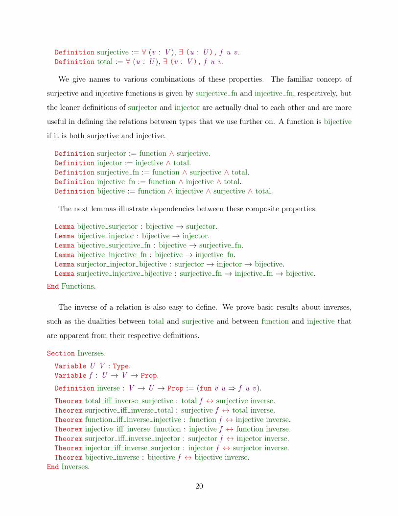
Definition surjective := ∀ (v : V ), ∃ (u : U ), f u v .Definition total := ∀ (u : U ), ∃ (v : V ), f u v .

We give names to various combinations of these properties. The familiar concept of

surjective and injective functions is given by surjective fn and injective fn, respectively, but

the leaner definitions of surjector and injector are actually dual to each other and are more

useful in defining the relations between types that we use further on. A function is bijective

if it is both surjective and injective.

Definition surjector := function ∧ surjective.Definition injector := injective ∧ total.Definition surjective fn := function ∧ surjective ∧ total.Definition injective fn := function ∧ injective ∧ total.Definition bijective := function ∧ injective ∧ surjective ∧ total.

The next lemmas illustrate dependencies between these composite properties.

Lemma bijective surjector : bijective → surjector.Lemma bijective injector : bijective → injector.Lemma bijective surjective fn : bijective → surjective fn.Lemma bijective injective fn : bijective → injective fn.Lemma surjector injector bijective : surjector → injector → bijective.Lemma surjective injective bijective : surjective fn → injective fn → bijective.

End Functions.

The inverse of a relation is also easy to define. We prove basic results about inverses,

such as the dualities between total and surjective and between function and injective that

are apparent from their respective definitions.

Section Inverses.

Variable U V : Type.Variable f : U → V → Prop.

Definition inverse : V → U → Prop := (fun v u ⇒ f u v).

Theorem total iff inverse surjective : total f ↔ surjective inverse.Theorem surjective iff inverse total : surjective f ↔ total inverse.Theorem function iff inverse injective : function f ↔ injective inverse.Theorem injective iff inverse function : injective f ↔ function inverse.Theorem surjector iff inverse injector : surjector f ↔ injector inverse.Theorem injector iff inverse surjector : injector f ↔ surjector inverse.Theorem bijective inverse : bijective f ↔ bijective inverse.

End Inverses.

20

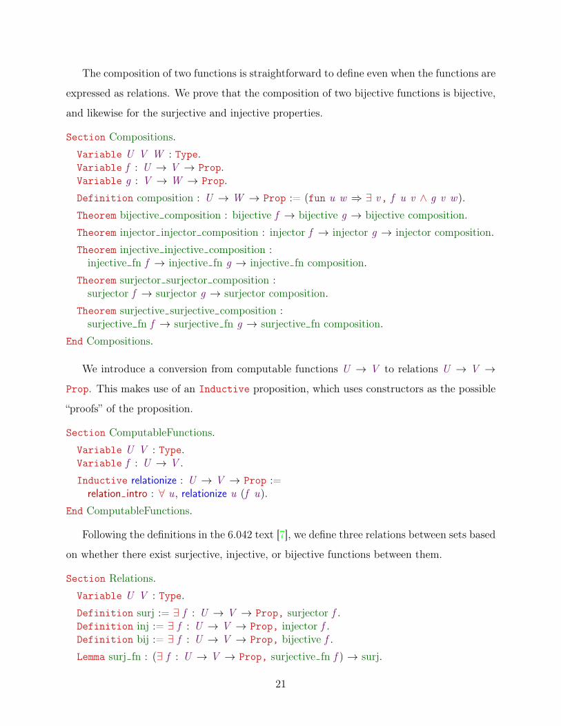
The composition of two functions is straightforward to define even when the functions are

expressed as relations. We prove that the composition of two bijective functions is bijective,

and likewise for the surjective and injective properties.

Section Compositions.Variable U V W : Type.Variable f : U → V → Prop.Variable g : V → W → Prop.Definition composition : U → W → Prop := (fun u w ⇒ ∃ v, f u v ∧ g v w).Theorem bijective composition : bijective f → bijective g → bijective composition.Theorem injector injector composition : injector f → injector g → injector composition.Theorem injective injective composition :injective fn f → injective fn g → injective fn composition.

Theorem surjector surjector composition :surjector f → surjector g → surjector composition.

Theorem surjective surjective composition :surjective fn f → surjective fn g → surjective fn composition.

End Compositions.

We introduce a conversion from computable functions U → V to relations U → V →

Prop. This makes use of an Inductive proposition, which uses constructors as the possible

“proofs” of the proposition.

Section ComputableFunctions.Variable U V : Type.Variable f : U → V .Inductive relationize : U → V → Prop :=relation intro : ∀ u, relationize u (f u).

End ComputableFunctions.

Following the definitions in the 6.042 text [7], we define three relations between sets based

on whether there exist surjective, injective, or bijective functions between them.

Section Relations.Variable U V : Type.Definition surj := ∃ f : U → V → Prop, surjector f .Definition inj := ∃ f : U → V → Prop, injector f .Definition bij := ∃ f : U → V → Prop, bijective f .Lemma surj fn : (∃ f : U → V → Prop, surjective fn f ) → surj.

21

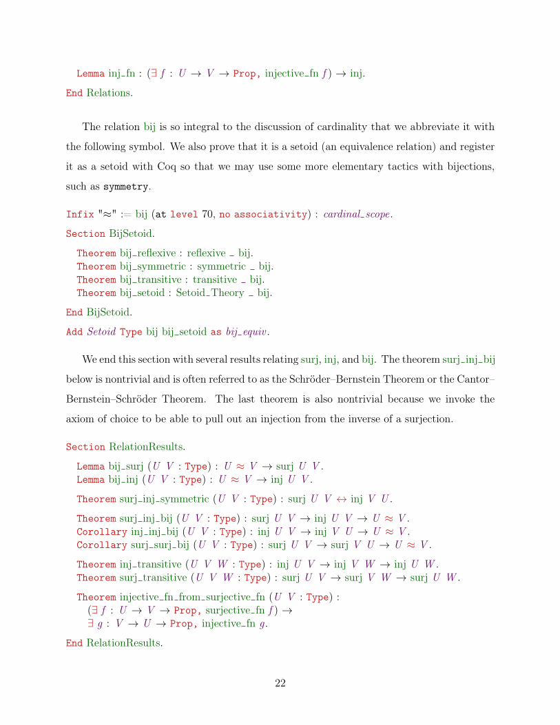
Lemma inj fn : (∃ f : U → V → Prop, injective fn f ) → inj.

End Relations.

The relation bij is so integral to the discussion of cardinality that we abbreviate it with

the following symbol. We also prove that it is a setoid (an equivalence relation) and register

it as a setoid with Coq so that we may use some more elementary tactics with bijections,

such as symmetry.

Infix "≈" := bij (at level 70, no associativity) : cardinal scope.

Section BijSetoid.

Theorem bij reflexive : reflexive bij.Theorem bij symmetric : symmetric bij.Theorem bij transitive : transitive bij.Theorem bij setoid : Setoid Theory bij.

End BijSetoid.

Add Setoid Type bij bij setoid as bij equiv .

We end this section with several results relating surj, inj, and bij. The theorem surj inj bij

below is nontrivial and is often referred to as the Schröder–Bernstein Theorem or the Cantor–

Bernstein–Schröder Theorem. The last theorem is also nontrivial because we invoke the

axiom of choice to be able to pull out an injection from the inverse of a surjection.

Section RelationResults.

Lemma bij surj (U V : Type) : U ≈ V → surj U V .Lemma bij inj (U V : Type) : U ≈ V → inj U V .

Theorem surj inj symmetric (U V : Type) : surj U V ↔ inj V U .

Theorem surj inj bij (U V : Type) : surj U V → inj U V → U ≈ V .Corollary inj inj bij (U V : Type) : inj U V → inj V U → U ≈ V .Corollary surj surj bij (U V : Type) : surj U V → surj V U → U ≈ V .

Theorem inj transitive (U V W : Type) : inj U V → inj V W → inj U W .Theorem surj transitive (U V W : Type) : surj U V → surj V W → surj U W .

Theorem injective fn from surjective fn (U V : Type) :(∃ f : U → V → Prop, surjective fn f ) →∃ g : V → U → Prop, injective fn g .

End RelationResults.

22

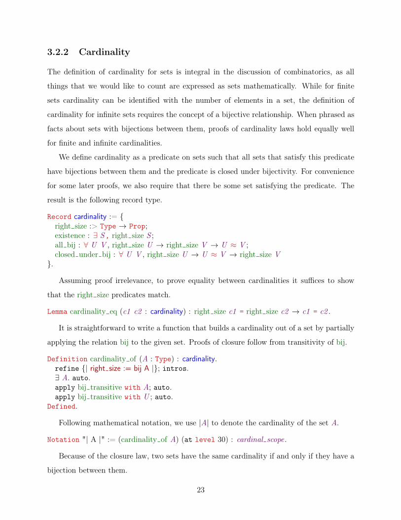
3.2.2 Cardinality

The definition of cardinality for sets is integral in the discussion of combinatorics, as all

things that we would like to count are expressed as sets mathematically. While for finite

sets cardinality can be identified with the number of elements in a set, the definition of

cardinality for infinite sets requires the concept of a bijective relationship. When phrased as

facts about sets with bijections between them, proofs of cardinality laws hold equally well

for finite and infinite cardinalities.

We define cardinality as a predicate on sets such that all sets that satisfy this predicate

have bijections between them and the predicate is closed under bijectivity. For convenience

for some later proofs, we also require that there be some set satisfying the predicate. The

result is the following record type.

Record cardinality := {right size :> Type → Prop;existence : ∃ S, right size S ;all bij : ∀ U V , right size U → right size V → U ≈ V ;closed under bij : ∀ U V , right size U → U ≈ V → right size V

}.

Assuming proof irrelevance, to prove equality between cardinalities it suffices to show

that the right size predicates match.

Lemma cardinality eq (c1 c2 : cardinality) : right size c1 = right size c2 → c1 = c2 .

It is straightforward to write a function that builds a cardinality out of a set by partially

applying the relation bij to the given set. Proofs of closure follow from transitivity of bij.

Definition cardinality of (A : Type) : cardinality.refine {| right size := bij A |}; intros.∃ A. auto.apply bij transitive with A; auto.apply bij transitive with U ; auto.

Defined.

Following mathematical notation, we use |A| to denote the cardinality of the set A.

Notation "| A |" := (cardinality of A) (at level 30) : cardinal scope.

Because of the closure law, two sets have the same cardinality if and only if they have a

bijection between them.

23

Lemma cardeq bij A B : |A| = |B | ↔ A ≈ B .

An example of a cardinality that we can write down now is that of the empty set.

Definition zero cardinal := |Empty set|.

The general definition of inequalities between cardinals depends on the inj and surj rela-

tions defined earlier. We say that |A| ≤ |B| if and only if there is an injection from A to B.

This yields the following definition on Coq cardinalities.

Definition cardinal le (c1 c2 : cardinality) :=∃ (A : Type), c1 A ∧ ∃ (B : Type), c2 B ∧ inj A B .

This definition of ≤ obeys the standard reflexivity and transitivity laws.

Lemma cardinal le reflexive : reflexive cardinal le.Lemma cardinal le transitive : transitive cardinal le.

The other inequality relations can be defined in terms of ≤.

Definition cardinal ge (c1 c2 : cardinality) := c2 ≤ c1 .Definition cardinal lt (c1 c2 : cardinality) := c1 ≤ c2 ∧ c1 6= c2 .Definition cardinality gt (c1 c2 : cardinality) := c2 < c1 .

For cardinals taken from specific sets A and B , we show that ≤ and ≥ are equivalent to

the relations inj and surj.

Theorem cardinal le inj A B : |A| ≤ |B | ↔ inj A B .Theorem cardinal ge surj A B : |A| ≥ |B | ↔ surj A B .

3.2.3 Finite Cardinalities

Nearly all cardinalities that we deal with in combinatorics are those of finite sets. We define

an injection from natural numbers to cardinalities using the “interval” of natural numbers

{x : nat | x < n} as the prototypical n-element set. We first define shorthand notation for

these finite intervals.

Definition interval (n : nat) := { x : nat | x < n }.Notation "[0 – n )" := (interval n).Notation "{ 0 , 1 }" := (interval 2).

Definition interval2 (m n : nat) := { x : nat | m ≤ x < n }.Notation "[ m – n )" := (interval2 m n).

24

We define n size to be the predicate for whether a Type is finite with exactly n elements.

Fixpoint n size (n : nat) (T : Type) : Prop :=match n with| 0 ⇒ T → False| S n’ ⇒ ∃ x : T, n size n’ { x’ : T | x’ 6= x }

end.

We prove that n size is closed under bij .

Theorem n size bij (n : nat) : ∀ (s1 s2 : Type), n size n s1 → n size n s2 → s1 ≈ s2 .Theorem n size closed (n : nat) : ∀ (U V : Type), n size n U → U ≈ V → n size n V .

The intervals defined above satisfy n size predicates.

Theorem n interval size (n : nat) : n size n [0, . . . ,n).Theorem n interval2 size (a b : nat) : n size (b - a) [a, . . . ,b).

We package together the n size predicate with its proofs of closure into cardinality n,

the injection from nat to cardinality.

Definition cardinality n (n : nat) : cardinality.refine ({| right size := n size n;

all bij := n size bij n;closed under bij := n size closed n |}).

∃ [0, . . . ,n).auto.

Defined.

Coercion cardinality n : nat −→ cardinality .

We have several easy lemmas about sets we already know that are equal to cardinality n

of various numbers.

Lemma empty set cardinality : zero cardinal = 0.Lemma interval cardinality (n : nat) : |[0, . . . ,n)| = n.Lemma interval2 cardinality (a b n : nat) : |[a, . . . ,b)| = b - a.

To show that cardinality n is injective, we show inductively that there cannot be any

bijection from interval m to interval n if m 6= n. The core of this proof is to show the

following lemma, constructing a bijection {0, . . . , a− 1} ↔ {0, . . . , b− 1} out of a bijection

{0, . . . a} ↔ {0, . . . , b}. This is done by tying together the element that maps from a and

the element that maps to b.

25

Lemma interval bijection peel (a b : nat) :interval (S a) ≈ interval (S b) → interval a ≈ interval b.

Lemma interval bijection ineq (m n : nat) : m < n → interval m 6≈ interval n.Theorem interval bijection eq (m n : nat) : interval m ≈ interval n → m = n.Corollary cardinality n equality (m n : nat) :cardinality n m = cardinality n n → m = n.

The inclusion map i : {0, . . . ,m− 1} ↪→ {0, . . . , n− 1} for m ≤ n gives us a quick proof

of the next fact.

Theorem cardinality n le (m n : nat) : m ≤ n → (m ≤ n)%cardinal .

It follows that < between naturals also carries over to < between cardinalities.

Theorem cardinality n lt (m n : nat) : m < n → (m < n)%cardinal .

A simple proof that a set has a certain cardinality is to exhaustively enumerate all of its

elements. The following section implements this proof strategy.

Section EnumeratedTypes.Variable S : Type.Variable enum : list S .Hypothesis enum NoDup : NoDup enum.Hypothesis enum total : ∀ (s : S ), In s enum.

We define the bijection between interval (length enum) and S using the nth error function

for indexing into lists.

Definition index enumeration (n : interval (length enum)) (s : S ) :=match nth error enum (proj1 sig n) with| Some x ⇒ x = s| None ⇒ False

end.

Lemma index enumeration bijective : bijective index enumeration.Theorem enumerated type : |S | = length enum.

End EnumeratedTypes.

We can then write an Ltac function to use the above theorem and prove some simple

examples.

Ltac enumeration l :=apply enumerated type with (enum := l);[ repeat (constructor; try (simpl; intuition; discriminate)) |let x := fresh in intro x ; destruct x ; simpl; tauto ].

26

Theorem unit sz : |unit| = 1.enumeration (tt :: nil).

Qed.

Lemma bool sz : |bool| = 2.enumeration (true :: false :: nil).

Qed.

3.2.4 Product and Sum of Cardinalities

We define the product of two cardinalities to be the following predicate.

Definition splits as product (c1 c2 : cardinality) (S : Type) :=∃ A : Type, ∃ B : Type, S ≈ (A × B) ∧ c1 A ∧ c2 B .

The × operator on types is defined to be the Cartesian product of the two types. We see

here that the set S satisfies splits as product c1 c2 if it can be decomposed as the product

of two sets whose cardinalities match c1 and c2 . As with other cardinalities, we prove that

this predicate is closed under bijections.

Lemma bij product (A B C D : Type) : A ≈ B → C ≈ D → A × C ≈ B × D .Lemma product cardinality all bij (c1 c2 : cardinality) (A B : Type) :splits as product c1 c2 A → splits as product c1 c2 B → A ≈ B .

Lemma product cardinality bij transitive (c1 c2 : cardinality) (A B : Type) :splits as product c1 c2 A → A ≈ B → splits as product c1 c2 B .

Definition product cardinality (c1 c2 : cardinality) : cardinality.refine {| right size := splits as product c1 c2;

all bij := @product cardinality all bij c1 c2;closed under bij := @product cardinality bij transitive c1 c2 |}.

...

Defined.

Infix "×" := product cardinality : cardinal scope.

We can show that the product cardinality behaves as we would expect on the Cartesian

product of sets. It also follows the symmetry and associativity laws that multiplication on

numbers follows.

Theorem product rule A B : |A × B | = |A| × |B |.Theorem product symmetric (c0 c1 : cardinality) : c0 × c1 = c1 × c0 .Theorem product associative (c0 c1 c2 : cardinality) : c0 × (c1 × c2) = (c0 × c1) × c2 .

27

Beyond following these product laws, product cardinality is compatible with the product

of natural numbers for cardinalities of finite sets. We show here that there is a bijection

f : {0, . . . ,m− 1} × {0, . . . , n− 1} → {0, . . . , (m− 1)(n− 1)} defined by

f(a, b) = a + mb.

Definition interval product map (m n : nat) (x : interval m × interval n)(y : interval (m × n)) := (proj1 sig (fst x ) + m × proj1 sig (snd x ))%nat = proj1 sig y .

Lemma interval product bijective : ∀ m n, bijective (@interval product map m n).Theorem nat product cardinality (m n : nat) :cardinality n m × cardinality n n = cardinality n (m × n).

With the product cardinality defined, we can prove Theorem 3.1.3 pertaining to sets

related by k-to-1 functions. Recall that a k-to-1 function is defined to be a function f : U →

V such that for each v ∈ V , there are exactly k elements in U which map to v. We write

this definition in Coq again using relations as functions.

Section Division.Variable U V : Type.Variable f : U → V → Prop.Definition k to 1 k := total f ∧ function f ∧ ∀ v : V , |{ u : U | f u v }| = k .

The theorem applies the product rule using V and a set K whose cardinality is k . We

use the axiom of choice (in a dependently typed version) to instantiate the bijection between

K and { u : U | f u v } for each v in V .

Theorem division rule k : k to 1 k → |U | = k × |V |.End Division.

We can use this division rule to prove a generalized version of the product rule using

dependently typed pairs rather than Cartesian product. Given a function f : T → Type

that associates a Type to every element in T , the type sigT f is the type of pairs whose first

element is some t in T and whose second element is of type f t . An alternative notation for

sigT is similar to that for normal sigma types: { t : T & f t }.

Section SigTProdRule.Variable T : Type.

28

Variable f : T → Type.Variable k : cardinality.Hypothesis regular : ∀ t : T , k = |f t |.Theorem sigT prod rule : |{ t : T & f t }| = k × |T |.

End SigTProdRule.

This dependently typed variation leads us to define the version of the product rule which

is actually used in the proof of the poker hand example at the beginning of the section.

Given a subset of a type T as a predicate P : T → Prop we can use a uniform projection

function Q to refine the cardinality of {t : T | P t} into a product |P’ | × |V |, where P’ is

the preimage of a specific value under Q and V is the set of possible values for Q . In the

first step of the full houses example, we use a projection function that maps a hand with

a full house to the rank of the triple in that hand. Naming this function r : H → R and

choosing a specific r̄, the set of full house hands then has cardinality

|H| = |{h ∈ H | r(h) = r̄}| × |R|.

This refines the problem because we know the size |R| by definition. In general, we can use

any k-to-1 function in place of r.

We also have an auxiliary definition here which is the restriction of a function to a subset

of its input.

Definition restrict T V (f : T → V → Prop) (S : T → Prop) :=fun (t : sig S ) (v : V ) ⇒ f (proj1 sig t) v .

Notation "( Q | P )" := (@restrict Q P).

Section GeneralProductRule.

Variable T V : Type.Variable P : T → Prop.Variable Q : T → V → Prop.

For convenience we let the projection function Q be defined in terms of the base set, but

we require that it be only defined on the subset P and be a total function on that set.

Hypothesis Q total function : function (Q | P) ∧ total (Q | P).Hypothesis Q defined on P : ∀ t v , Q t v → P t .

First, we show that the set of pairs (v, t) where t ∈ Q−1(v) is in bijection with the

elements of P . This bijection is simply (Q(t), t)↔ t.

29

Theorem projection size : { v : V & { t : T | Q t v } } ≈ { t : T | P t }.Corollary projection cardinality :|{ v : V & {t : T | Q t v} }| = |{t : T | P t}|.

Variable k : cardinality.Hypothesis gen regular : ∀ v : V , k = |{ t : T | Q t v }|.

Given that Q is k-to-1, we can apply sigT prod rule to find that the set of pairs (v, t)

above has cardinality k|V |. This along with projection cardinality gives our final rule. The

reason that we don’t use the earlier k to 1 definition here is because we are phrasing Q as a

function of T rather than sig T , so the entire Q is not actually a total function. Avoiding the

sigma type helps in reducing the boilerplate sigma projections and constructor uses needed

to apply this rule.

Lemma gen product rule pair : |{ v : V & {t : T | Q t v} }| = k × |V |.Theorem gen product rule : |{t : T | P t}| = k × |V |.

End GeneralProductRule.

The sum of two cardinalities is defined analogously to product, using disjoint sum of sets

rather than Cartesian product. Unsurprisingly, the + operator on types in Coq is already

defined to be the disjoint sum. We use the following predicate on types.

Definition splits as sum (c1 c2 : cardinality) (S : Type) :=∃ s1 : Type, ∃ s2 : Type, S ≈ (s1 + s2) ∧ c1 s1 ∧ c2 s2 .

With this, we can define sum cardinality as we have done with product cardinality.

Lemma bij sum (A B C D : Type) : A ≈ B → C ≈ D → A + C ≈ B + D .Lemma sum cardinality all bij (c1 c2 : cardinality) (A B : Type) :splits as sum c1 c2 A → splits as sum c1 c2 B → A ≈ B .

Lemma sum cardinality bij transitive (c1 c2 : cardinality) (A B : Type) :splits as sum c1 c2 A → A ≈ B → splits as sum c1 c2 B .

Definition sum cardinality (c1 c2 : cardinality) : cardinality.refine {| right size := splits as sum c1 c2;

all bij := @sum cardinality all bij c1 c2;closed under bij := @sum cardinality bij transitive c1 c2 |}.

...

Defined.

Infix "+" := sum cardinality : cardinal scope.

30

Analogues to the theorems we have about product cardinality also hold about sum cardinality.

Theorem sum rule (s1 s2 : Type) : |s1 + s2 | = |s1 | + |s2 |.Theorem sum symmetric (c0 c1 : cardinality) : c0 + c1 = c1 + c0 .Theorem sum associative (c0 c1 c2 : cardinality) : c0 + (c1 + c2) = (c0 + c1) + c2 .

The map that we use similarly to the interval product map earlier is the bijection

f : {0, . . . ,m− 1} t {0, . . . , n− 1} → {0, . . . ,m + n− 2} defined as the bijection

{0, . . . ,m− 1} t {0, . . . , n− 1} ≈ {0, . . . ,m− 1} t {m, . . . ,m + n− 2}.

In code, this is

Definition interval sum map (m n : nat) (x : interval m + interval n)(y : interval (m + n)) := match x with

| inl a ⇒ proj1 sig a = proj1 sig y| inr b ⇒ (m + proj1 sig b)%nat = proj1 sig y

end.

Lemma interval sum bijective : ∀ m n, bijective (@interval sum map m n).

Theorem nat sum cardinality (m n : nat) :cardinality n m + cardinality n n = cardinality n (m + n).

We can use sum cardinality to break up a set { s : S | P x } into two disjoint subsets

based on some predicate (Q : S → Prop). The initial set may or may not itself be represented

as a subset.

Theorem sum split (S : Type) (P Q : S → Prop) :|{ x | P x }| = |{ x | P x ∧ Q x }| + |{ x | P x ∧ ¬ Q x }|.

Corollary sum split full set (S : Type) (Q : S → Prop) :|S | = |{ x | Q x }| + |{ x | ¬ Q x }|.

We can relate product cardinality to sum cardinality with the normal distributivity laws.

The case of c + c = 2 × c is a useful special case, but we also prove distributivity in its full

generality.

Lemma sum cardinality diag (c : cardinality) : c + c = 2 × c.Theorem cardinality distrib l (a b c : cardinality) : a × (b + c) = a × b + a × c.Corollary cardinality distrib r (a b c : cardinality) : (a + b) × c = a × c + b × c.

We may even prove some interesting facts about infinite cardinalities. For example, the

set of integers Z satisfies |Z| = |Z| + |Z|, using the following bijection.

31

Lemma zip bijection : bijective (fun (n : Z) (p : Z + Z) ⇒match p with| inl m ⇒ m + m = n| inr m ⇒ m + m + 1 = n

end).Theorem Z equals Z plus Z : |Z| = |Z| + |Z|.

Using the definitions of product and sum cardinality, we may also investigate the cardi-

nalities of power sets. Since an element of Ensemble T for a type T is a subset of T , the

type Ensemble T is the power set of the type T . If |T | = n, the power set P(T ) has 2n

elements. First, we show that the set P({0, . . . , n − 1}) has 2n elements. This is using the

standard proof by induction: the power set P({0, . . . , n}) splits in half based on whether the

element n is in a given subset, and each half is in bijection with a subset of {0, . . . , n− 1}.

We invoke sum cardinality diag above (the fact that c + c = 2 × c) to make use of this.

Theorem interval power set n : |Ensemble [0–n)| = 2ˆn.

After this, we can extend the theorem to all finite sets T , because if |T | = n then we have

a bijection between T and the discrete n-element interval. The only remaining interesting

part of the proof of this power set rule is that if two sets have the same cardinality, then

their power sets also have the same cardinality.

Lemma equal power sets T T’ : |T | = |T’ | → |Ensemble T | = |Ensemble T’ |.Theorem power set rule T (n : nat) : |T | = n → |Ensemble T | = 2ˆn.

3.2.5 Cardinalities of Subsets

We wish to write down rules about cardinalities of subsets of types, using Ensemble and

sig. Given a list of elements that makes up a subset, if the list has no duplicates then the

cardinality of this subset is equal to the length of the list.

Theorem cardinal of list A (l : list A) : NoDup l → |sig (list to subset l)| = length l .

Corollary subset length match T (l l’ : list T ) :l ∼= l’ → NoDup l → NoDup l’ → length l = length l’ .

The notation (l ∼= l’ ) here expands to (list to subset l) = (list to subset l’ ). Next we

have several basic lemmas about empty, nonempty, and singleton sets.

32

Lemma empty subset empty T : |sig (Empty set T )| = 0.

Lemma single empty subset T : ∀ x : Ensemble T , |sig x | = 0 → Empty set T = x .

Theorem single subset T (P : Ensemble T ) : (∃! x : T, P x ) → |sig P | = 1.

Theorem no subsets T (P : Ensemble T ) : (¬ ∃ x : T, P x ) → |sig P | = 0.

Lemma empty type T : |T | = 0 → T → False.

Lemma nonempty type T : ∀ n, |T | = S n → ∃ t : T, True.

Given that there’s a bijection between two sets A and B , we can find a bijection that

maps some specific a ∈ A to a given b ∈ B.

Lemma bijective wlog A B (a : A) (b : B) (f : A → B → Prop) :bijective f → ∃ f ’ : A → B → Prop, bijective f ’ ∧ f ’ a b.

Removing an element from a finite subset that it’s in (or from the whole set) results in

a set that is smaller by one. Removing an element from a subset that it’s not in does not

change the size of the subset.

Theorem remove element subset T (s : Ensemble T ) :∀ n, |sig s| = S n → ∀ t : T , s t → |{x : T | s x ∧ x 6= t}| = n.

Corollary remove element T : ∀ n, |T | = S n → ∀ t : T , |{x : T | x 6= t}| = n.

Lemma remove element not in subset T (s : Ensemble T ) :∀ n, |sig s| = n → ∀ t , (¬ s t) → |{x | s x ∧ x 6= t}| = n.

We often want to consider subsets of a particular size only. For example, poker hands

are subsets of the set of cards that have size 5. For this, we have the following definition.

Definition sized subset (T : Type) (n : cardinality) :={ x : Ensemble T | |sig x | = n }.

Definition in set T n (S : sized subset T n) (x : T ) := x ∈ proj1 sig S .

We can rephrase the Ensemble theorem Extensionality Ensembles in terms of sized subset

to have a criterion for when sized subsets are equal.

Lemma sized subset extensionality T n (A B : sized subset T n) :(∀ x , in set A x ↔ in set B x ) → A = B .

The cardinality of the type of sized subset for a particular size is also of interest. For

finite sets, this cardinality is a binomial coefficient.

Definition choose cardinal (T : Type) (k : cardinality) := |sized subset T k |.

33

A simple way to define binomial coefficients in Coq is using the recursive formula(n

k

)=

(n− 1

k

)+

(n− 1

k − 1

).

Fixpoint choose nat (n k : nat) : nat :=match k with| O ⇒ 1| S k’ ⇒ match n with

| O ⇒ O| S n’ ⇒ (choose nat n’ k’ + choose nat n’ k)%nat

endend.

Notation "( n ’choose’ k )" := (choose nat n k).Notation "n !" := (fact n) (at level 15).

The binomial defined in this manner is equal to the common factorial definition(n

k

)=

n!

k!(n− k)!.

Theorem choose factorial (n k : nat) : k ≤ n → n! = (n choose k) × k! × (n - k)!.

The major result here is that the number of k-element subsets of a set T with cardinality

n is equal to(nk

). The standard argument for why this cardinality is equal to the recursive

definition of(nk

)goes as follows. If T is empty, we are in the base case. Otherwise, we fix

an element t ∈ T and divide up the k element subsets into those which contain t and those

which do not. The subsets which contain t are in bijection with subsets of T \ {t} that have

k−1 elements and the subsets which do not contain t are in bijection with subsets of T \{t}

that have k elements.

Theorem choose equal (n : nat) :∀ T , |T | = n → ∀ k : nat, choose cardinal T k = (n choose k).

3.3 Automating Counting Proofs

To arrive at the automation of the proof steps that we see in the example from the beginning

of the section, we went through applying the proof steps by hand. For brevity, we have a

34

slightly smaller example here that we investigate. This proof is calculating the number of

three-card hands of cards there are given that there is exactly one pair in the hand. Before

the proof, we have the definitions of the data types involved. Ranks and suits are defined

simply as enumerated inductive types. A card is a pair with a rank and a suit.

Inductive Rank := RA | R2 | R3 | R4 | R5 | R6 | R7 | R8 | R9 | R10 | RJ | RQ | RK.Inductive Suit := Clubs | Diamonds | Hearts | Spades.Definition Card := (Rank × Suit)%type.

We have the two projection functions out of Card.

Definition rank := @fst Rank Suit.Definition suit := @snd Rank Suit.

There are easy proofs of the cardinalities of Rank and Suit because they follow directly

from the definitions.

Lemma Rank sz : |Rank| = 13.enumeration (RA :: R2 :: R3 :: R4 :: R5 :: R6 :: R7 :: R8 ::R9 :: R10 :: RJ :: RQ :: RK :: nil).

Qed.Lemma Suit sz : |Suit| = 4.enumeration (Clubs :: Diamonds :: Hearts :: Spades :: nil).

Qed.Hint Rewrite Rank sz Suit sz : cardinality .

We write a tactic for automatically proving the size of compound data types, using

the cardinality hint database. This tactic knows about simplifying sets that have elements

removed, binomial coefficient sizes, and sum and product cardinalities.

Ltac prove size :=repeat rewrite product rule;try (erewrite remove element subset; [reflexivity | prove size | auto]);try (erewrite remove element; [reflexivity | prove size]);try (match goal with

| [ ` context[|sized subset ?T ?n|] ] ⇒ fold (choose cardinal T n)| ⇒ idtac

end; erewrite choose equal; [reflexivity | prove size]);autorewrite with cardinality;reflexivity || apply nat product cardinality || apply nat sum cardinality

This can prove the cardinality of Card, given that the cardinalities of Rank and Suit have

been entered into the hint database.

35

Lemma Card sz : |Card| = 52.unfold Card.prove size.

Qed.

Hint Rewrite Card sz : cardinality .

Definition compute size S := { size | |S | = size }.

For cardinality proofs where we do not know the size of the set beforehand, we may phrase

the size as a sigma type. A goal of compute size T means that we are both computing some

cardinality and proving that it equals |T |.

Now we arrive at the proof. We describe the “having a pair” criterion as two cards sharing

a rank and the third having a different rank. The notation used, which we have seen in the

example of Section 3.1, will be defined in Section 3.4.

Definition has pair := (3 6→ rank‘ $0 = rank‘ $1 ∧ rank‘ $0 6= rank‘ $2)%nary .Arguments has pair /.

Theorem pair size : compute size { S : Ensemble Card | ex set S 3 has pair }.

The way that we express the exercise of rigorously computing a value without knowing it

beforehand is captured in the definition of compute size. We can reduce our goal to the proof

part of the sigma type by using eexists to instantiate the value part with an existential

variable.

Proof.eexists.

Here, our goal is

============================|{S : Ensemble Card |ex set S 3 (rank ‘ $0 = rank ‘ $1 ∧ rank ‘ $0 6= rank ‘ $2)} | = ?39

We want to apply Theorem 3.1.3, that is, use the gen product rule. Our first projection

function is going to be to take the shared rank of the pair. The way we write this function

is as follows.

erewrite gen product rule with (Q :=(fun (S : Ensemble Card) (r : Rank) ⇒ex set S 3 (has pair ∧ (, r) = rank‘ $0 ))).

36

The , notation is simply a lift of a constant to a constant function and is explained in

more detail in Section 3.4. Because Q is defined over the base type (here Ensemble Card)

rather than over the subset { S : Ensemble Card | ex set S 3 has pair }, we have to specify

in Q that its argument S satisfies the same properties that are already in the goal. However,

setting this up the other way would lead to a more difficult problem: given an Ensemble

Card that we know satisfies the ex set criterion in the original goal, we cannot easily write

down exactly what is the rank of the pair in that subset. The cards in the subset are only

given an ordering inside of the existential covered by ex set, so writing it in the above form

actually allows us to use the references $0, etc., to write the projection function.

Applying gen product rule leaves us with four subgoals:

• The total cardinality is equal to the refined cardinality times the cardinality of the

image of Q .

• The restriction of the function Q to the set we project out of (in this case, three-card

hands containing one pair) is a well-defined and total function.

• Q is only defined on this set and not on other subsets of Card.

• Calculate the refined cardinality.

The first of these subgoals does not really require proof so much as it is asking us to relate

the previous existential variable with the new existential variable that erewrite generated for

the refined cardinality. The goal is

============================?92 × |Rank| = ?39

We simplify the cardinality |Rank| and then use reflexivity to tell Coq that this is

exactly the relationship between the two existentials.

autorewrite with cardinality .reflexivity.

In the second subgoal, we begin by splitting up the “function” and “total” propositions

that come from the Q total function hypothesis.

37

simpl. split.

The first of these, well-definedness, is one of the most involved parts of the proof. We

begin tackling this by doing some surface simplification and pulling out the hypotheses.

hnf. simpl.intros (z , Hz ) x y Hx Hy . simpl in *. clear Hz .

Our subgoal is now

z : Ensemble Cardx : Ranky : RankHx : ∃ x0 x1 x2 : Card,

[x0 ; x1 ; x2 ] enumerates z ∧rank x0 = rank x1 ∧ rank x0 6= rank x2 ∧ x = rank x0

Hy : ∃ x x0 x1 : Card,[x ; x0 ; x1 ] enumerates z ∧rank x = rank x0 ∧ rank x 6= rank x1 ∧ y = rank x

============================x = y

The notation [x0 ; x1 ; x2 ] is simply shorthand for the list x0 :: x1 :: x2 :: nil . This

subgoal is asking us to show that given two ranks x and y that are each the projection of Q off

of a subset z , the ranks must be the same. We first reduce the complexity of the hypotheses

Hx and Hy by instantiating the Cards as variables and pulling off the “enumerates” facts

into their own hypotheses.

repeat match type of Hx with| ∃ , ⇒ destruct Hx as (?, Hx )

end.destruct Hx as (Henum, Hx ).

repeat match type of Hy with| ∃ , ⇒ destruct Hy as (?, Hy)

end.destruct Hy as (Henum’ , Hy).

simpl in *.

Then we deconstruct the rest of the hypotheses and eliminate extra variables.

repeat (subst; intuition).

This cleans up the subgoal to look as follows.

38

z : Ensemble Cardx0 : Cardx1 : Cardx2 : CardHenum : [x0 ; x1 ; x2 ] enumerates zx3 : Cardx4 : Cardx5 : CardHenum’ : [x3 ; x4 ; x5 ] enumerates zH : rank x0 = rank x1H1 : rank x3 = rank x4H3 : rank x0 = rank x2 → FalseH0 : rank x3 = rank x5 → False============================rank x0 = rank x3

The interesting part of this proof is that we can tell that [x0 ; x1 ; x2 ] is some permutation

of [x3 ; x4 ; x5 ], but they do not necessarily map one-to-one. We need to prove that if the

variables have been permuted but still satisfy the set specification, then the rank of the

first element is unchanged. One approach could be to consider all permutations of the list

[x0 ; x1 ; x2 ]. Unfortunately, performing the resulting proof search in every branch becomes

intractible for larger problems such as full poker hands of five cards. Instead, we aim to

cut this search space by only considering permutations which actually satisfy has pair in

their ordering. In this case, the first two elements of a hand can be swapped and the hand

will still satisfy has pair, but no other permutations are valid. A more generalizable way

of expressing this is that the equivalence relation (fun (x y : Card) ⇒ rank x = rank y)

partitions the hand into a set of equivalence classes. When permuting the list, elements

that were equivalent must remain equivalent. Hence, a valid permutation of the list sends

one equivalence class to a permutation of another class. In the case of [x0 ; x1 ; x2 ], which

partitions into [x0 ; x1 ] ++ [x2 ], the two equivalence classes have distinct sizes so they must

map to themselves.

assert (Heq0 : EquivPartitioned (fun x y ⇒ rank x = rank y)[x0; x2] [[x0; x1]; [x2]])

by (hnf; split; [ go | prove NoEquiv ]).replace [x0; x1; x2] with (flatten ([[x0; x1]; [x2]])) in Henum by reflexivity.

assert (Heq1 : EquivPartitioned (fun x y ⇒ rank x = rank y)[x3; x5] [[x3; x4]; [x5]])

39

by (hnf; split; [ go | prove NoEquiv ]).replace [x3; x4; x5] with (flatten ([[x3; x4]; [x5]])) in Henum’ by reflexivity.

eapply enumerate symmetry in Heq0 ; [ | | simpl; eauto | apply Heq1 ]; [ | auto ].simpl in Heq0 . clear Heq1 .rewrite flatten fold app in *.

After applying enumerate symmetry , we have added

Heq0 : [ [x3 ; x4 ]; [x5 ] ] ∼= [ [x0 ; x1 ]; [x2 ] ]

to our set of hypotheses. Recall that l ∼= l’ means (list to subset l) = (list to subset

l’ ), so the two lists are permutations of each other. This reduces our search to permutations

of this list of two elements, rather than the larger list. In other cases, like the full houses

example, reducing the search space from 5! to 2! possibilities is a significant difference. We

have a specific tactic to do a case analysis of the different possible permutations.

destruct permutations Heq0 .

In the first case, we break up Heq0 into

H1 : [x0 ; x1 ] ∼= [x3 ; x4 ]H2 : [x2 ] ∼= [x5 ]

This is the correct matching. In order to show that rank x0 = rank x3 , given that rank

x0 = rank x1 above, we look at the two cases of permutations given by H1 and can solve

them with subst and intuition.

destruct permutations H1 ; subst; intuition.

In the second case, we have

H1 : [x2 ] ∼= [x3 ; x4 ]H2 : [x0 ; x1 ] ∼= [x5 ]

Two subsets can only be permutations of each other if, given that their enumerations do

not have repetitions, the enumerations have the same length. We apply this logic to H1 ,

and then we must prove that both lists satisfy the NoDup property. This is not too difficult.

We have that [x3 ; x4 ; x5 ] enumerates z implies NoDup [x3 ; x4 ; x5 ] and that [x3 ; x4 ] is a

sublist of a list with no duplicates. We earlier rewrote the list [x3 ; x4 ; x5 ] as (flatten [ [x3 ;

x4 ]; [x5 ] ]) which lets us do this unification easily.

40

apply subset length match in H1 ; [ discriminate | | ];destruct Henum; destruct Henum’ .

eapply NoDup in fold app; [ | apply H6 ]. subst; intuition.eapply NoDup in fold app; [ | apply H8 ]. subst; intuition.

This finishes the subgoal that Q is well-defined. The next subgoal is to prove that Q is

defined on all sets that satisfy has pair.

hnf. intros [x Hx ]. simpl.

After some simplification, our goal is

x : Ensemble CardHx : ∃ x0 x1 x2 : Card,

[x0 ; x1 ; x2 ] enumerates x ∧ rank x0 = rank x1 ∧ rank x0 6= rank x2============================∃ (v : Rank) (x0 x1 x2 : Card),[x0 ; x1 ; x2 ] enumerates x ∧(rank x0 = rank x1 ∧ rank x0 6= rank x2 ) ∧ v = rank x0

The goal is basically already in the hypothesis Hx . We instantiate the Card variables in

the goal with the Cards from Hx , repeatedly using the fact

∃x,∃y, P x y → ∃y,∃x, P x y

to push the ∃ (v : Rank) back to the end. We then turn v into an existential and are able

to prove the rest of goal with first-order logic.

destruct Hx as [c0 Hx ]. apply exists swap. ∃ c0 . simpl.destruct Hx as [c1 Hx ]. apply exists swap. ∃ c1 . simpl.destruct Hx as [c2 Hx ]. apply exists swap. ∃ c2 . simpl.

eexists.firstorder; firstorder.

Now we have shown that Q is defined on all sets with has pair. Next we must show that

these are the only sets on which it is defined.

intro. intro. simpl.

This goal has a parallel structure much like the previous, but is easier because we don’t

need to figure out what the rank v is.

t : Ensemble Card

41

v : Rank============================(∃ x x0 x1 : Card,

[x ; x0 ; x1 ] enumerates t ∧(rank x = rank x0 ∧ rank x 6= rank x1 ) ∧ v = rank x ) →

∃ x x0 x1 : Card,[x ; x0 ; x1 ] enumerates t ∧ rank x = rank x0 ∧ rank x 6= rank x1

Here we invoke Coq’s tactic for solving goals that are simply first-order logic.

firstorder.

Finally, we arrive at our last subgoal, which is to calculate the cardinality of the refined

set.

intro r .

Once we pull the fixed variable up into our hypotheses, we now have to calculate the

number of subsets with this r fixed.

============================∀ v : Rank,?61 = |{t : Ensemble Card | ex set t 3 (has pair ∧ ( , v) = rank ‘ $ 0)} |

The remaining choices of projections are very similar, so we skip them here by using our

automation. There are a few interesting problems that we run into in these cases that are

not in this first projection. The second projection is onto ranks other than r , rather than

all ranks, so we need to involve a sigma type {r’ | r’ 6= r} that we need to destruct at

the appropriate times. In the sized subset case, we additionally run into goals similar to

[suit x0 ; suit x1 ] ∼= [suit x3 ; suit x4 ]. Here we have [x0 ; x1 ] ∼= [x3 ; x4 ] as above, so we

use the lemma list to subset map, which shows that we can apply map on both sides of the

permutation (∼=) expression.

pose (card hint [2; 1]).pick r’ as (3 6→ rank‘ $2) from {r’ | r’ 6= r}.pick s as (3 6→ set[ suit‘ $0; suit‘ $1 ]) from (sized subset Suit 2).pick s’ as (3 6→ suit‘ $2).

name all .

Now what remains to show is that these choices of ranks and suits determine a single

subset.

42

symmetry. apply single subset. simpl.

The subgoal we have is

r : Rankp := card hint [2; 1] : PokerHintr’ : RankH : r’ 6= rs : Ensemble Suits’ : Suits0 : SuitH1 : s s0s1 : SuitH3 : s s1H5 : [s0 ; s1 ] enumerates s============================∃ ! x : Ensemble Card,∃ x0 x1 x2 : Card,[x0 ; x1 ; x2 ] enumerates x ∧((((rank x0 = rank x1 ∧ rank x0 6= rank x2 ) ∧ r = rank x0 ) ∧r’ = rank x2 ) ∧ s = [suit x0 ; suit x1 ]) ∧

s’ = suit x2

Let us refer to the subset specification as P , so that this goal has the form ∃ ! x :

Ensemble Card, P x . We can write down the unique subset satisfying P using the fixed

variables in our hypotheses.

∃ [(r, s0); (r, s1); (r’, s’)].unfold unique. split.

To prove uniqueness, first we prove that the given subset does actually satisfy P , and

then we must prove that it is the only such subset which does. In the list we have specified

our elements in the same order that they appear in has pair, so we use these to instantiate

the next three existentials.

∃ (r, s0). ∃ (r, s1). ∃ (r’, s’). simpl.split.

The first section of the proposition is

[(r , s0 ); (r , s1 ); (r’ , s’ )] enumerates [(r , s0 ); (r , s1 ); (r’ , s’ )]

Clearly the lists are equal, so we are left with proving

43

NoDup [(r , s0 ); (r , s1 ); (r’ , s’ )]

This follows from the hypotheses H : r’ 6= r and H5 : [s0 ; s1 ] enumerates s . We have

a short tactic that encapsulates the proof of NoDup.

split; [ auto | t NoDup ].

After this, the rest of the proposition follows easily. The only part that intuition cannot

solve immediately is that H5 : [s0 ; s1 ] enumerates s implies s = [s0 ; s1 ], which we get by

destructing H5 .

intuition.destruct H5 . assumption.

The second part of the uniqueness proof is that the supplied subset is in fact the only

subset which satisfies P . Given some other subset, result , that satisfies P , we need to prove

that it is equal to ours, or that the list representation is a permutation of our list [(r , s0 );

(r , s1 ); (r’ , s’ )]. We start by simplifying the hypothesis (P result).

intros result H’ .destruct H’ as [c0 H’ ].destruct H’ as [c1 H’ ].destruct H’ as [c2 H’ ].destruct H’ as [Henum H’ ].destruct Henum as [Henum]. rewrite Henum. clear Henum. clear result .

repeat match goal with| [ H : ∧ ` ] ⇒ destruct H ; subst| [ H : |sig (list to subset )| = ` ] ⇒ clear H

end.

After simplification, the goal becomes

p := card hint [2; 1] : PokerHints0 : Suits1 : Suitc0 : Cardc1 : Cardc2 : CardH0 : NoDup [c0 ; c1 ; c2 ]H2 : rank c0 = rank c1H4 : rank c0 6= rank c2H1 : [suit c0 ; suit c1 ] s0H3 : [suit c0 ; suit c1 ] s1

44

H5 : [s0 ; s1 ] enumerates [suit c0 ; suit c1 ]H : rank c2 6= rank c0============================[(rank c0 , s0 ); (rank c0 , s1 ); (rank c2 , suit c2 )] ∼= [c0 ; c1 ; c2 ]

One way to prove that these two lists are permutations of each other could be to consider

all of the possible permutations. Since this case split is much slower when the size of the

Ensemble is bigger, we turn again to the fact that when permuting the elements of our

set, the only valid permutations come from permuting elements in appropriately defined

equivalence classes. We transform this goal into a stronger one where we have to prove both

that [(rank c0 , s0 ); (rank c0 , s1 )] ∼= [c0 ; c1 ] and [(rank c2 , suit c2 )] ∼= [c2 ].

let li := constr:[2; 1] inmatch goal with| ` ?l0 ∼= ?l1 ⇒replace l0 with (flatten (separate list li l0 )) by reflexivity;replace l1 with (flatten (separate list li l1 )) by reflexivity;simpl separate list in *; apply sublist permutation equality ; simpl

end.

In order to prove the first of these, we need to leverage the hypotheses H2 : rank c0 =

rank c1 and H5 : [s0 ; s1 ] enumerates [suit c0 ; suit c1 ]. It would be possible to go through

and destruct every Card in the subgoal, but such a strategy does not easily generalize to

when we want to count arbitrary data types. A slightly more general principle we invoke

here is the following.

Lemma refine permutation A B C (f : A → B) (g : A → C ) (l l’ : list A) :(∀ x y , f x = f y → g x = g y → x = y) →∀ y , Forall (fun x ⇒ f x = f y) (l ++ l’ ) →map g l ∼= map g l’ →l ∼= l’ .

Given two projection functions f and g out of a type A, the fact that equality under f

and equality under g together yield equality in A and the fact that all the elements of our

lists are equal under f , then we can weaken our goal to map g l ∼= map g l’ . We apply this

here with rank as f and suit as g .

constructor.eapply (refine permutation (hint f p) (hint g p)); simpl.go.

45

repeat constructor; simpl; auto.destruct H5 . symmetry. assumption.

constructor.eapply (refine permutation (hint f p) (hint g p)); simpl.go.repeat constructor; simpl; auto.auto.

constructor.Defined.

This finishes an unautomated version of the proof for the number of three-card sets which

have exactly one pair.

Eval simpl in (proj1 sig pair size).

= 1 × 4 × 6 × 12 × 13: cardinality

Coincidentally, this is the same as the number of poker hands with full houses because(41

)=(43

).

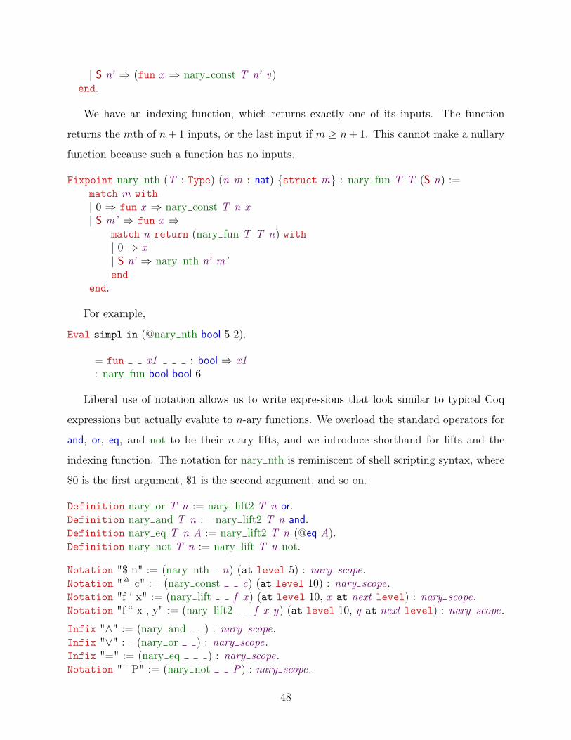
3.4 n-ary Function Notation

One of the issues in applying gen product rule in counting proofs is that we need to restate

the subset definition in order to add conditions inside of the existential. Unfortunately, it

is very difficult to use the Ltac term matching mechanism to match and rewrite inside of

several existential qualifiers in our use case. In order to save users from having to rewrite

the entire subset definition, we develop here a monadic notation for writing functions that

take a number of parallel inputs. The type (nary fun T V n) represents the type

T → · · · → T︸ ︷︷ ︸n

→ V.

Fixpoint nary fun (T V : Type) (n : nat) : Type :=match n with| 0 ⇒ V| S n’ ⇒ T → nary fun T V n’

46

end.

An nary prop is just a Prop-valued n-ary function.

Definition nary prop T n := nary fun T Prop n.

We have an existential quantifier for n-ary propositions. This prepends an ∃ (x : T ) to

the front of the given proposition for each input that it takes.

Fixpoint nary ex T n (P : nary prop T n) : Prop :=match n return nary prop T n → Prop with| 0 ⇒ fun P’ : nary prop T 0 ⇒ P’| S n’ ⇒ fun P’ : nary prop T (S n’ ) ⇒∃ x : T, nary ex T n’ (P’ x )

end P .

A variant of nary ex, nary ex pred prepends ∃ (x : T ), Q x ∧ .. for each variable,

allowing an additional specification to be put on each input.

Fixpoint nary ex pred T n (Q : T → Prop) (P : nary prop T n) : Prop :=match n return nary prop T n → Prop with| 0 ⇒ fun P’ : nary prop T 0 ⇒ P’| S n’ ⇒ fun P’ : nary prop T (S n’ ) ⇒∃ x : T, Q x ∧ nary ex pred n’ Q (P’ x )

end P .

Functions can be lifted to be compositions with n-ary functions. We define lifts of unary

and binary functions, as well as lifts of constants into constant functions.

Fixpoint nary lift T V V’ n (f : V → V’ ) :nary fun T V n → nary fun T V’ n :=match n return nary fun T V n → nary fun T V’ n with| 0 ⇒ f| S n’ ⇒ fun A x ⇒ nary lift T n’ f (A x )

end.

Fixpoint nary lift2 T V V’ V’’ n (f : V → V’ → V’’ ) :nary fun T V n → nary fun T V’ n → nary fun T V’’ n :=match n return nary fun T V n → nary fun T V’ n → nary fun T V’’ n with| 0 ⇒ f| S n’ ⇒ fun A B x ⇒ nary lift2 T n’ f (A x ) (B x )

end.

Fixpoint nary const T V n (v : V ) : nary fun T V n :=match n return nary fun T V n with| 0 ⇒ v

47

| S n’ ⇒ (fun x ⇒ nary const T n’ v)end.

We have an indexing function, which returns exactly one of its inputs. The function

returns the mth of n + 1 inputs, or the last input if m ≥ n + 1. This cannot make a nullary

function because such a function has no inputs.

Fixpoint nary nth (T : Type) (n m : nat) {struct m} : nary fun T T (S n) :=match m with| 0 ⇒ fun x ⇒ nary const T n x| S m’ ⇒ fun x ⇒

match n return (nary fun T T n) with| 0 ⇒ x| S n’ ⇒ nary nth n’ m’end

end.

For example,

Eval simpl in (@nary nth bool 5 2).

= fun x1 : bool ⇒ x1: nary fun bool bool 6

Liberal use of notation allows us to write expressions that look similar to typical Coq

expressions but actually evalute to n-ary functions. We overload the standard operators for

and, or, eq, and not to be their n-ary lifts, and we introduce shorthand for lifts and the

indexing function. The notation for nary nth is reminiscent of shell scripting syntax, where

$0 is the first argument, $1 is the second argument, and so on.

Definition nary or T n := nary lift2 T n or.Definition nary and T n := nary lift2 T n and.Definition nary eq T n A := nary lift2 T n (@eq A).Definition nary not T n := nary lift T n not.

Notation "$ n" := (nary nth n) (at level 5) : nary scope.Notation ", c" := (nary const c) (at level 10) : nary scope.Notation "f ‘ x" := (nary lift f x ) (at level 10, x at next level) : nary scope.Notation "f “ x , y" := (nary lift2 f x y) (at level 10, y at next level) : nary scope.

Infix "∧" := (nary and ) : nary scope.Infix "∨" := (nary or ) : nary scope.Infix "=" := (nary eq ) : nary scope.Notation "˜ P" := (nary not P) : nary scope.

48

Notation "a <> b" := (¬ (a = b))%nary : nary scope.

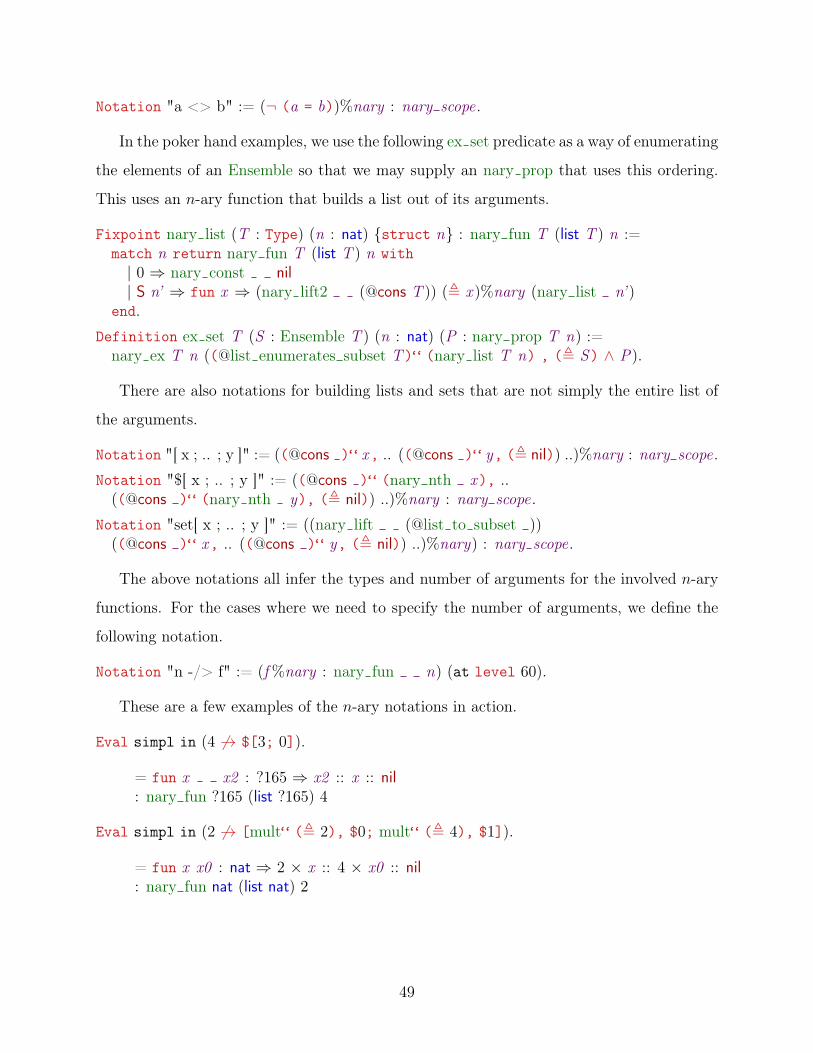
In the poker hand examples, we use the following ex set predicate as a way of enumerating

the elements of an Ensemble so that we may supply an nary prop that uses this ordering.

This uses an n-ary function that builds a list out of its arguments.

Fixpoint nary list (T : Type) (n : nat) {struct n} : nary fun T (list T ) n :=match n return nary fun T (list T ) n with| 0 ⇒ nary const nil| S n’ ⇒ fun x ⇒ (nary lift2 (@cons T )) (, x )%nary (nary list n’ )

end.

Definition ex set T (S : Ensemble T ) (n : nat) (P : nary prop T n) :=nary ex T n ((@list enumerates subset T)“ (nary list T n) , (, S) ∧ P).

There are also notations for building lists and sets that are not simply the entire list of

the arguments.

Notation "[ x ; .. ; y ]" := ((@cons )“ x, .. ((@cons )“ y, (, nil)) ..)%nary : nary scope.

Notation "$[ x ; .. ; y ]" := ((@cons )“ (nary nth x), ..((@cons )“ (nary nth y), (, nil)) ..)%nary : nary scope.

Notation "set[ x ; .. ; y ]" := ((nary lift (@list to subset ))((@cons )“ x, .. ((@cons )“ y, (, nil)) ..)%nary) : nary scope.

The above notations all infer the types and number of arguments for the involved n-ary

functions. For the cases where we need to specify the number of arguments, we define the

following notation.

Notation "n -/> f" := (f%nary : nary fun n) (at level 60).

These are a few examples of the n-ary notations in action.

Eval simpl in (4 6→ $[3; 0]).

= fun x x2 : ?165 ⇒ x2 :: x :: nil: nary fun ?165 (list ?165) 4

Eval simpl in (2 6→ [mult“ (, 2), $0; mult“ (, 4), $1]).

= fun x x0 : nat ⇒ 2 × x :: 4 × x0 :: nil: nary fun nat (list nat) 2

49

50

Chapter 4

Probability

Probability theory, like counting, has a strong focus in the 6.042 curriculum. Some work has

also been done to express basic concepts of probability in Coq. However, we have not begun

automation for these types of problems.

Most probability exercises are similar to combinatorial exercises in that they ask for

computations of values with justification. However, these values are probabilities rather

than cardinalities. The premises for probability problems are generally more involved than

those in combinatorics because they usually describe a probability distribution over some

space of events. Questions that test knowledge of infinite probability spaces sometimes have

even more complicated setups, often involving games or processes that repeat with some

random chance.

4.1 Probability Example

The following simple example exercise is taken from the 6.042 textbook [7]. The proof shows

the reasoning a student might be expected to explain.

Exercise 4.1.1. What’s the probability that 0 doesn’t appear among k digits chosen inde-

pendently and uniformly at random?

Proof. For any given digit, the probability Pr[digit i is nonzero] is 9/10. Since the digits are

51

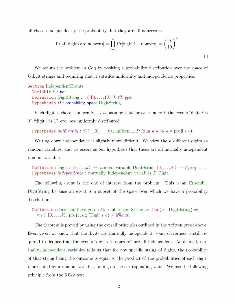
all chosen independently the probability that they are all nonzero is

Pr[all digits are nonzero] =k∏

i=1

Pr[digit i is nonzero] =

(9

10

)k

.

We set up the problem in Coq by positing a probability distribution over the space of

k-digit strings and requiring that it satisifes uniformity and independence properties.

Section IndependentEvents.Variable k : nat.Definition DigitString := ( [0, . . . ,10)ˆk )%type.Hypothesis D : probability space DigitString.

Each digit is chosen uniformly, so we assume that for each index i, the events “digit i is

0”, “digit i is 1”, etc., are uniformly distributed.

Hypothesis uniformity : ∀ i : [0, . . . ,k), uniform D (fun a b ⇒ a = proji i b).

Writing down independence is slightly more difficult. We view the k different digits as

random variables, and we assert as our hypothesis that these are all mutually independent

random variables.

Definition Digit : [0, . . . ,k) → random variable DigitString [0, . . . ,10) := @proji .Hypothesis independence : mutually independent variables D Digit.

The following event is the one of interest from the problem. This is an Ensemble

DigitString because an event is a subset of the space over which we have a probability

distrbution.

Definition does not have zero : Ensemble DigitString := fun (a : DigitString) ⇒∀ i : [0, . . . ,k), proj1 sig (Digit i a) 6= 0%nat .

The theorem is proved by using the overall principles outlined in the written proof above.

Even given we know that the digits are mutually independent, some cleverness is still re-

quired to deduce that the events “digit i is nonzero” are all independent. As defined, mu-

tually independent variables tells us that for any specific string of digits, the probability

of that string being the outcome is equal to the product of the probabilities of each digit,

represented by a random variable, taking on the corresponding value. We use the following

principle from the 6.042 text.

52

Lemma 4.1.2. Let Q : T→ X and R : T→ X’ be independent random variables, and assume

we have functions f : X→ Y and g : X’→ Y’. Then f(Q) and g(R) are independent random

variables.

Using the function (fun (d : interval 10) ⇒ beq nat (proj1 sig d) 0), which produces

a boolean value for whether the digit is equal to zero, we convert the independent random

variables for the digits into independent random variables for whether the digits are equal

to zero. The hypothesis of uniformity gives us that one value for these random variables is

1/10, so the other must be 9/10. The product of the k variables gives us the result.

Theorem Pr of does not have zero : Pr D does not have zero = ( (9/10)ˆk )%Qc.End IndependentEvents.

4.2 Probability Foundations

A probability space is a probability function on a space of outcomes bundled with a proof

that it is always nonnegative and that it sums to one. We choose to make this probability

function take values in Qc (the set of rational numbers in lowest terms) because it is much

easier to compute over Q than over R, and nearly all probability functions we would consider

in discrete math only take on rational values. The notation (sum pr w for w : space) is

a formal sum that packages together its index set and summands, and the notation s 7→ v

means that the formal sum s evaluates to v . Sums taken over finite sets can be evaluated,

but we have not yet implemented evaluation of infinite series.

Record probability space (space : Type) := {pr : space → Qc ;pr nonnegative : ∀ w : space, 0 ≤ pr w ;pr normalized : (sum pr w for w : space) 7→ 1

}.

We can define a simple example of a probability space: one which is defined on the first

n naturals and where each outcome has probability 1/n. The proof that this is a probability

space is relatively straightforward using compute. We have a slightly roundabout method

53

that distinguishes between s 7→ v and eval s because not all sums are necessarily computable,

and the notation eval s implicitly infers an enumeration of the index set of s . This is done

using the Type Class feature in Coq.

Definition ex uniform n (x : [0, . . . ,n)) := 1 / n.Definition ex space3 : probability space [0, . . . ,3).refine {| pr := @ex uniform 3 |}; go.match goal with| [ ` ?s 7→ ?v ] ⇒replace v with (eval s) by (compute; apply Qc is canon; reflexivity)

end.apply finite evaluation.

Defined.

We can define what it means for a space generally to be uniform, and show that our

example space is indeed uniform.

Definition uniform space {T} (sp : probability space T ) := ∃ q, ∀ w , pr sp w = q .

Lemma ex space3 uniform : uniform space (ex space3).

More generally, for a finite uniform space T , the probability of each outcome happening

is 1/|T |. Here we see the use of Type Classes as the parameter ‘{Finite T} is an inferrable

parameter.

Theorem uniform space probability T (sp : probability space T ) ‘{Finite T} :uniform space sp → ∀ t , pr sp t = 1 / (size of T).

There is a distinction between events and outcomes. A probability function is defined on

a space of outcomes. An event is a subset of the space of outcomes, whose probability (with

a capital “P”) is defined to be the sum of the probabilities of the outcomes in the event.

Section Events.

Variable T : Type.Variable sp : probability space T .

Definition formal Pr (E : Ensemble T ) : formal sum T Qc := sum of E (pr sp).

Though we define the probability of an event as a formal sum, we would like a definition

which allows us to manipulate probabilities as actual rational numbers, rather than purely

formally. We can do this using Hilbert’s epsilon operator, which is an extension that in-

stantiates an element satisfying a given property, if one exists. If one does not, the epsilon

54

operator returns some arbitrary element of that type (it is justified in doing so because

epsilon requires a proof that the type is inhabited). The epsilon operator can be thought

of as a computational version of the axiom of choice; assuming its validity allows us to

deterministically instantiate an element of a set.

Definition Pr (U : Ensemble T ): Qc :=epsilon (inhabits 0) (fun v ⇒ (sum (pr sp u) for u in U ) 7→ v).

If the formal sum has an evaluation, then Pr returns it, and sums over finite sets can

always be evaluated.

Theorem exists Pr a (U : Ensemble T ): formal Pr U 7→ a → Pr U = a.

Theorem eval Pr (U : Ensemble T ) ‘{Finite (sig U )} : formal Pr U 7→ Pr U .

Formally, if we can evaluate probability over two events, then we can evaluate probability

over the union of these two events. If the events are disjoint, then the probability over them

is the sum of the two probabilities of the events.

Theorem formal Pr disjoint union (U V : Ensemble T ) a b :formal Pr U 7→ a → formal Pr V 7→ b →Disjoint U V → formal Pr (U ∪ V ) 7→ a + b.

Using the epsilon version of Pr, we can write this in a more algebraic fashion.

Theorem Pr disjoint union (U V : Ensemble T ) ‘{Finite (sig U )} ‘{Finite (sig V )} :Disjoint U V → Pr U + Pr V = Pr (U ∪ V ).

As a direct corollary, we can apply the law (U ∩ V ) ∪ (U ∩W ) = U ∩ (V ∪W ).

Corollary Pr intersection sum (U V W : Ensemble T )‘{Finite (sig (U ∩ V ))} ‘{Finite (sig (U ∩ W ))} :Disjoint V W → Pr (U ∩ V ) + Pr (U ∩ W ) = Pr (U ∩ (V ∪ W )).

The complement law is another consequence of the disjoint union law because a set and

its complement are disjoint, their union is the entire space, and the total probability over

the space is 1. Here, we use U c to denote the complement of U in T .

Theorem Pr complement sum (U : Ensemble T ) ‘{Finite (sig U )} ‘{Finite T} :Pr U + Pr (U c) = 1.

This rule can be rewritten in terms of subtraction as well.

Corollary Pr complement (U : Ensemble T ) ‘{Finite (sig U )} ‘{Finite T} :Pr (U c) = 1 - Pr U .

55

There are several other probability laws in this spirit which follow from rules about

operations on sets, including facts about set difference (U \ V = {x | x ∈ U ∧ x 6∈ V }) and

the principle of inclusion–exclusion.

Theorem Pr setminus (U V : Ensemble T ) ‘{Finite (sig U )} ‘{Finite (sig V )} :Pr (U \ V ) = Pr U - Pr (U ∩ V ).

Theorem Pr PIE (U V : Ensemble T ) ‘{Finite (sig U )} ‘{Finite (sig V )} :Pr U + Pr V - Pr (U ∩ V ) = Pr (U ∪ V ).

Theorem Pr monotonic (U V : Ensemble T ) : U ⊂ V → Pr U ≤ Pr V .

Lemma Pr empty set : Pr (Empty set ) = 0.

Corollary Pr bounded below (U : Ensemble T ) : 0 ≤ Pr U .

Theorem Pr bounded above (U : Ensemble T ) ‘{Finite T} ‘{Finite (sig U )} : Pr U ≤ 1.

We also define a notion of uniform distribution of events rather than outcomes. A set of

events Ej for j in some index set J are uniform if they are mutually disjoint, they cover the

entire outcome space, and they all have equal probability. As with outcomes, we can show

that the probability of one of J uniform events is 1/|J |.

Definition uniform {J} (E : J → Ensemble T ) :=(∀ i j , Disjoint (E i) (E j )) ∧(∀ t , ∃ t’, Ensembles.In (E t’ ) t) ∧∃ p, ∀ t’ , Pr (E t’ ) = p.

Theorem uniform probability {J} ‘{Finite J} (E : J → Ensemble T ) :uniform E → ∀ j , Pr (E j ) = 1 / (size of J).

End Events.

Another central concept in probability is conditional probability, which is straightforward

to define from the definition of Pr.

Section Conditionals.

Variable T : Type.Variable sp : probability space T .Notation "Pr[ U ]" := (@Pr T sp U ) (at level 50, U at next level).

Definition CondPr (U V : Ensemble T ) := Pr[U ∩ V ] / Pr[V ].Notation "Pr[ U | V ]" := (CondPr U V )(at level 50, U at next level, V at next level).

There are many laws which hold about conditional probability as well. Note that

Pr[U | V ] is not well-defined if Pr[V ] is zero.

56

Theorem CondPr bounded (U V : Ensemble T ) : Pr[V ] 6= 0 → 0 ≤ Pr[U | V ] ≤ 1.

Theorem Bayes rule (U V : Ensemble T ) :Pr[U ] 6= 0 → Pr[V ] 6= 0 → Pr[U | V ] = Pr[V | U ] × Pr[U ] / Pr[V ].

Theorem Total probability (U V : Ensemble T )‘{Finite T} ‘{Finite (sig U )} ‘{Finite (sig V )} :Pr[V ] 6= 0 → Pr[V ] 6= 1 →Pr[U ] = (Pr[U | V ] × Pr[V ]) + (Pr[U | V c] × Pr[V c]).

Two events are independent if conditioning one on the other does not change its proba-

bility. Equivalently, they are independent if the probability of both events happening is the

product of their respective probabilities.

Definition independent (U V : Ensemble T ) := Pr[U | V ] = Pr[U ].

Theorem independent Intersection (U V : Ensemble T ) :Pr[V ] 6= 0 → (independent U V ↔ Pr[U ∩ V ] = Pr[U ] × Pr[V ]).

As long as both events have nonzero probability, this notion of independence is commu-

tative.

Theorem independent comm (U V : Ensemble T ) :Pr[U ] 6= 0 → Pr[V ] 6= 0 → independent U V → independent V U .

A set of events Ej is pairwise independent if each pair of events is independent. A set

of events is mutually independent, a stronger assertion, if the intersection of any subset of

them factors as the product of the probabilities of the events in that subset.

Definition pairwise independent {J} (E : J → Ensemble T ) :=∀ i j , i 6= j → independent (E i) (E j ).

Definition mutually independent {J} (E : J → Ensemble T ) :=∀ js : list J , NoDup js →let events := map E js inPr[ Intersection list events ] = product over list (Pr sp) events .

End Conditionals.

Finally, we have the notion of random variables. These are simply functions on the

outcome space, typically projections of some compound outcome.

Section RandomVariables.

Variable T : Type.Variable sp : probability space T .

Variable X : Type.

57

Definition random variable := T → X .

Notation "[ R = x ]" := (fun space elt ⇒ R space elt = x )(R at level 50, x at level 50).

This notation is the event that the random variable R takes on the value x . Random

variables are independent if for any choice of values, the events that the variables take on

these values are independent. There is a corresponding notion of mutual independence.

Definition independent variables (R0 R1 : random variable) :=∀ x0 x1 : X , independent sp [R0 = x0] [R1 = x1].

Definition mutually independent variables {J} (R : J → random variable) :=∀ f : J → X , mutually independent sp (fun j ⇒ [(R j) = (f j)]).

End RandomVariables.

The principle used in the probability example at the beginning of the section can be writ-

ten in the following manner, generalizing to sets of mutually independent random variables

rather than pairs. The first theorem uses a different mapping for each random variable,

while the second is just a specialization for when we wish to apply the same mapping to each

variable.

Theorem map independent variables {T J X Y } (sp : probability space T )(R : J → random variable T X ) (f : J → X → Y ) :mutually independent variables sp R →mutually independent variables sp (fun j ⇒ (fun t ⇒ (f j ) (R j t))).

Corollary map independent variables’ {T J X Y } (sp : probability space T )(R : J → random variable T X ) (f : X → Y ) :mutually independent variables sp R →mutually independent variables sp (fun j ⇒ (fun t ⇒ f (R j t))).

58

Chapter 5

Future Research

The work developed here can continue to be extended with more concept definitions, more

exercises, and more proof automation. Making the automation increasingly robust is an

area that will require heavy focus in the future. Since we eventually want different levels of

detail for proofs over the course of a class like 6.042, perhaps additional abstract methodology

should be considered for developing automation for different sections of the class. There may

also be a need for designing an interface so that students do not have to interact directly

with a Coq front end. Right now, we envision using creative definitions of notation in Coq,

as with the n-ary function notation, to make it easier to write an intepreter that translates

proofs of some sort into Coq code. Ideally, students could write proofs in plain English that

the software would be able to verify. However, this direction is itself a difficult problem in

natural language processing.

Issues related more immediately to the work developed in this project include additional

topics within combinatorics and probability that merit attention and analysis. Common com-

binatorial concepts that remain to be implemented include uses of the pigeonhole principle

and various identities involving binomial coefficients. We also want better ways to describe

counting arguments in edge cases similar to examples we have developed. For instance, when

counting poker hands with three of a kind we want to use “the suit of the single card with

lower rank” and “the suit of the single card with higher rank” as projections, which might be

easier to do with better notation. In probability, we need to combine notions of conditionals

and independence to write down problems such as the classic Monty Hall problem. There

59

are a variety of other topics we have not yet covered in probability as well, such as infinite

probability spaces, expected values, and variance.

Overall, there is considerable research and implementation left to be finished before these

Coq libaries can be tested in the classroom. However, it will definitely be possible to craft

Coq exercises in the spirit of many existing paper exercises, especially if we are willing to

restrict the overall scope of the exercise set.

60

Bibliography

[1] David Aspinall. Proof General. http://proofgeneral.inf.ed.ac.uk/.

[2] Yves Bertot. Pcoq: A graphical user-interface for Coq. http://www-sop.inria.fr/

lemme/pcoq/.

[3] Carl Eastlund, Dale Vaillancourt, and Matthias Felleisen. ACL2 for Freshmen: First

Experiences. ACL2 Workshop, 2007.

[4] Georges Gonthier. Formal Proof — The Four-Color Theorem. Notices of the American

Mathematical Society, 55(11):1382–1393, 2008.

[5] Frédérique Guilhot. Formalisation en Coq et visualisation d’un cours de géométrie pour

le lycée. Technique et Science informatiques, 24(9):1113–1138, 2005.

[6] Matt Kaufmann and J. Strother Moore. ACL2. http://www.cs.utexas.edu/~moore/

acl2/. Version 4.3.

[7] Eric Lehman, F. Thomson Leighton, and Albert R. Meyer. Mathematics for Computer

Science.

[8] The Coq Development Team. The Coq Proof Assistant. LogiCal Project, 2013. Version

8.4.

[9] The Coq Development Team. The Coq Proof Assistant Reference Manual. LogiCal

Project, 2013. Version 8.4.

61