EARTH SURFACE PROCESSES AND LANDFORMS, VOL. 20, 13 1-1 37 (1995)

AUTOMATED MAPPING OF LAND COMPONENTS FROM DIGITAL ELEVATION DATA

J. R. DYMOND, R. C. DEROSE AND G. R. HARMSWORTH

Manaaki Whenua - Landcare Research, Privare Bag 11052, Palmersron North. New Zealand

Received 22 February 1993 Revised 14 March 1994

ABSTRACT

An algorithm for automating the mapping of land components from digital elevation data is described. Land components are areas of relatively uniform slope and aspect and often correspond with ridge crests, shoulders, head slopes, back slopes or foot slopes. Aspect regions, which generally span from stream to ridge, are first identified by generalizing an aspect map derived from digital elevation data. The aspect regions are then split successively into land components by grouping pixels above or below an automatically determined contour of elevation or ‘distance from stream’. The contour approximates a slope break. The land components mapped in this way give a complete polygonization of a hilly landscape and are a reason- able approximation of manually mapped land components.

KEY WORDS: land component; digital elevation‘ data; landform mapping

INTRODUCTION

Mapping of landforms in geomorplk analysis has traditionally been done using stereoscopic interpretation of aerial photographs. This manual method is slow and labour intensive. Now that digital elevation data, or digital terrain models (DTMs), are becoming more available, automated methods of landform mapping are being investigated in order to speed up landform mapping and reduce costs.

A number of authors have developed automatic methods to identify various singular terrain features: valley heads by Tribe (1 99 1); streams by Mark (1 984), O’Callaghan and Mark (1 984), Palacios-Velez and Cuevas-Renaud (1986) and Tarboton et al. (1991); ridges by Dymond (1992) and Riazanoff et al. (1988); watersheds by Jensorl and Domingue (1988), Jones et al. (1990) and Band (1986); and strike ridges and flu- vial deposits by Chorowicz et al. (1989). However, no progress has yet been reported on general landform recognition which would enable a landscape to be completely and automatically subdivided into its consti- tuent landforms. This is largely attributable to the mathematical complexity involved in representing land- form shape.

The land resources of New Zealand have been mapped at a scale of 1:63 360 by manually identifying and drawing polygon boundaries around resource units, using stereo aerial photographs. For each resource unit, rock type, soil type, vegetation, slope angle, erosion and an assessment of land use capability are recorded (National Water and Soil Conservation Organisation, 1979). The polygons have relatively uni- form resource attributes and hence similar land management requirements. The multifactor polygon method is very data efficient and has permitted all of New Zealand to be mapped and stored in an ARC/ INFO geographic information system. The database has proved to be an invaluable aid to regional planners nationwide. Yet there is a need for more detailed information. Regional planners have expressed a desire for the land units to be further subdivided and resource attributes determined for the more numerous land components, to facilitate planning at farm scales. The extra detail of mapping multiplies many times the

CCC 0197-9337/95/02013 1-07 0 1995 by John Wiley & Sons, Ltd

132 J. R. DYMOND, R. C. DEROSE AND G. R. HARMSWORTH

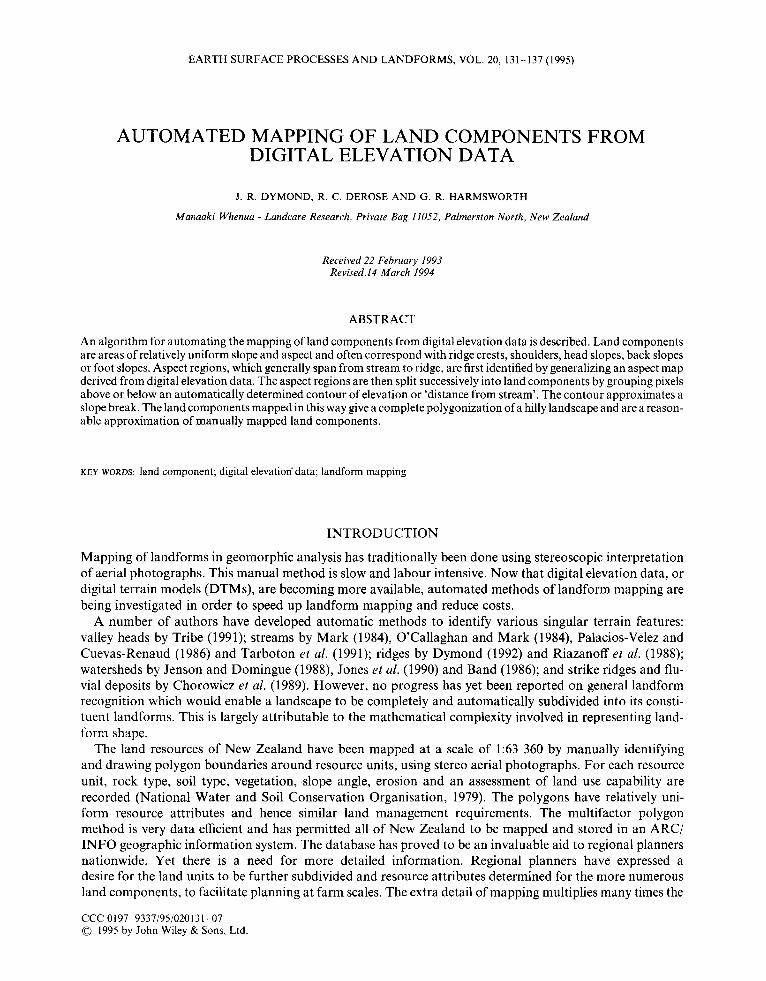
Figure 1. Data flow of algorithm that produces land components from digital elevation data

MAPPING OF LAND COMPONENTS 133

effort required and provides the motivation for developing a method for automatic mapping of land components.

Following earlier work by Christian (1 983), Harmsworth et al. (1992) conceptualized the landscape as a hierarchical assemblage of landforms comprising (from largest to smallest) land regions, land systems, land units, land components and land elements. Land units are usually synonymous with landforms, typically portrayed at scales between 150 000 and 1:25 000. Land elements are the smallest practical unit at a given scale of mapping; for a raster DTM this would be the pixel (Lamb et al., 1987), and for a triangulated irregular network (TIN) DTM it would be a DeLaunay triangle (McCullagh, 1988). The land component is an intermediate subdivision and typically is associated with ridge crests, shoulders, head slopes, back- slopes and foot slopes (Gerrard, 1990). Land components are usually mapped at scales between 15000 and 1 :25 000. Although land units are difficult to map automatically, because of difficulties in recognizing surface shape, it is possible to develop algorithms to automatically map land components as they are essen- tially areas of homogeneous aspect and slope.

This paper describes the implementation of an algorithm which automatically maps land components from a raster DTM.

ALGORITHM

The algorithm essentially identifies areas of land that have approximately constant aspect and slope. It begins as shown in Figure 1, with a per pixel classification of an aspect image into nine different aspect classes (eight aspect classes of 45" each and an additional class of pixels with slope angles below 4"). The aspect classification performs a good first cut of the landscape, as shown in Figure 1, regionalizing many major land units that stretch from ridge to stream. This classification, however, also produces many regions that are much smaller than typical land components, which need to be dissolved. This is done by finding all the regions below a given size (e.g. 100 pixels) and, for each small region in turn, replacing all the pixels in it with the most commonly occurring aspect on the perimeter of the region (using four connectivity as described by Gonzalez and Wintz, 1987). Pixels on the perimeter of a small region that are streams or ridges, or are touching streams or ridges in the small region, are not included in the calculation for the most commonly occurring aspect on the perimeter. This prevents aspect regions from going across stream or ridge boundaries.

The generalized aspect regions are then split into lower and upper slopes, where there is a significant dif- ference in the slope angles. A given elevation threshold, which separates the upper from the lower slopes, is varied between the minimum and the maximum elevation in the aspect region, in order to find the best poten- tial split. If there is a significant difference between the upper and lower slope angles at the best potential split, then the aspect region splits into two separate land components. This process is repeated, permitting seven types of land component: (1) main slope, (2) upper slope, (3) lower slope, (4) upper lower slope, (5) lower lower slope, (6) upper upper slope, and (7) lower upper slope.

The key to the algorithm is doing the split on an attribute that varies slowly in space (hence preserving the lumping of the pixels into regions) and upon which slope angles have a strong dependence. The attributes 'elevation' and 'distance from stream' both satisfy the requirements and are candidates for use.

GENERALIZING ASPECT

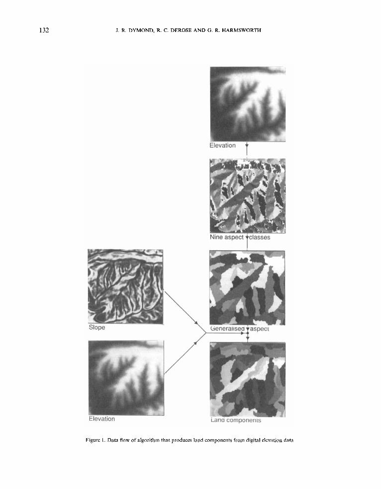
We generalized the aspect regions using a region growing algorithm similar to that described by Bailey (1991) and Gonzalez and Wintz (1987). Each aspect region in turn is scanned and all regions below a given area (1 00 pixels) are replaced with the most commonly occurring aspect on the perimeter, using four connectivity. Pix- els on the perimeter of the small region that are streams or ridges, or are touching streams and ridges in the small region, are excluded from the calculation of the most commonly occurring pixel. An example is worked in Figure 2. This exclusion rule prevents aspect regions from going across stream or ridge boundaries.

Streams and ridges can be extracted from a flow accumulation image (Jenson and Domingue, 1988) which gives the catchment area above any pixel in the DTM. Streams are defined as all pixels with flow

134 J. R. DYMOND, R. C . DEROSE AND G . R. HARMSWORTH

Figure 2. Example of dissolving a small region of Is where the numbers in bold italics occur on a ridge. Number of 2s on the perimeter = (total 4) ~ (2 ridges) - ( I touching ridge) = 1. Number of 3s on perimeter. = 3. No of 4s on perimeter = 1 . Most common on perimeter

are 3s, therefore replace Is with 3s

accumulation exceeding a given catchment area and ridges as all pixels with zero flow accumulation. Although the ridge network, mapped in this way, will include many minor ridges (Dymond, 1992), this is not critical to the generalization.

The generalizing program may need to be run several times before all the small regions are dissolved. This is usually the case when the aspect data are noisy and many small aspect regions cluster together. In this circumstance, many of the small regions in a cluster merely become assigned to one of the small aspect regions in the cluster after the first generalization. Towards the end of the generalization it may also be necessary to drop the rule which excludes ridges and boundaries in the calculation of the most commonly occurring aspect on the perimeter, so that all small aspect regions are successfully dissolved.

SLOPE DIVISION

Splitting of aspect regions into upper and lower slopes requires either elevation or ‘distance from stream’ data. For this section we will assume that the slope division is based on elevation data. Within a given aspect region, upper slope pixels separate from lower slope pixels, on the basis of being either greater or less than a given elevation, which we call the split elevation. The split elevation is varied at an appropriate interval (e.g. every 5 m) from the minimum to the maximum in the aspect region, to find the split that gives the great- est difference between upper and lower slope angles. Minimizing the average variance gives the greatest dif- ference where:

1 ’11

Average variance = - S,)2 + c ( S 1 - $)* / (nL , + nl) I = 1

where S, is the slope angle of an upper slope pixel, s, is the mean slope angle of the upper slope pixels, SI is the slope angle of a lower slope pixel, s1 is the mean slope angle of the lower slope pixels, nu is the number of upper slope pixels and nl is the number of lower slope pixels.

The split elevation value that gives the smallest average variance is then evaluated to see if the difference between the upper and lower slope angles is significant. The aspect region is then divided into upper and lower land components at this elevation, provided that:

(a) (average variance) < O.l*(no split variance); and (b) nl > 100 and nl > (nl + n,)/20; and (c) nu > 100 and 1 2 , > (nl + nu)/20.

where the no split variance is the total variance of upper and lower slope angles.

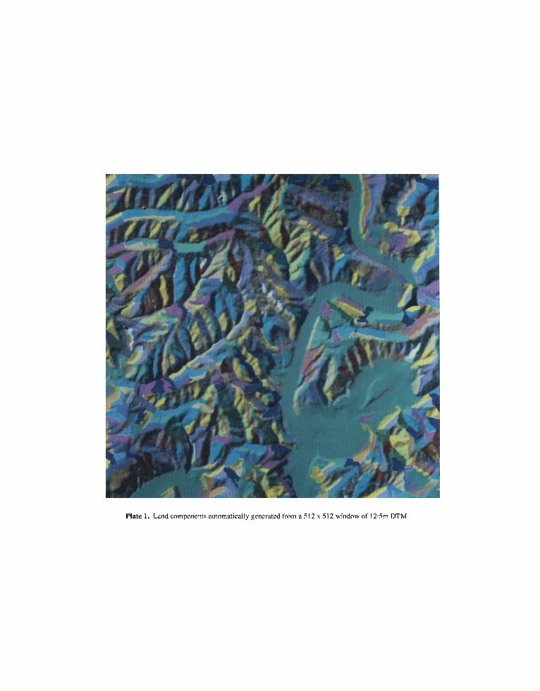
Plate 1. Land components automatically generated from a 512 x 512 window of 12.5m DTM

MAPPING OF LAND COMPONENTS 135

The variance reduction threshold of 0.1 may be made smaller if the algorithm produces too many land components. The minimum size of a land component may also be varied, both as an absolute value (100 used here) and as a fraction of the total aspect region size (lj20 used here).

The conditions above are satisfactory where only one split of the aspect region is needed, that is, where only an upper and lower land component exist. However, where three or four land components exist in the aspect region, then a further split of land components is required. To facilitate a double splitting procedure, the following conditions, if satisfied, also permit the most promising split to be effected as an alternative to the earlier condition:

(a) (upper slope variance) < O.l*(no split variance) or

(b) nl > 100 and nl > (nl + n,)/20; and (c) nu > 100 and nu > (nl + nu)/20.

These conditions permit a split which separates one land component from several others. After running the splitting procedure twice, there are seven possible types of land component: main slope,

upper slope, lower slope, lower or upper upper slope, and lower or upper lower slope. These seven types combine with the 13 aspect classes to form 91 possible land component codes.

(lower slope variance) < O.l*(no split variance); and

RESULTS

We ran the algorithm on two DTMs described by Dymond et al. (1992) and visually evaluated the resulting land component maps.

The Wanganui DTM was produced from 20 m digital contours, which were interpolated using an algo- rithm described by Letts and Rochon (1980) to produce a 12.5m raster DTM. An analytical stereoplotter was used to capture the contours from stereo aerial photographs. We applied the algorithm described in this paper to a 512 by 512 window of the DTM using eight aspect classes and using the attribute elevation to split the slopes (Plate 1).

The land components are realistic and give a complete subdivision of the landscape. Often they corre- spond with ridge crests, shoulders, head slopes, back slopes or foot slopes. Ridges and streams occur pre- cisely on land component boundaries. However, slope breaks are mapped approximately only, as they are constrained to lie along contour lines, which is not always the case in reality. Nevertheless, the land com- ponents compare reasonably well to those that would be mapped from stereoscopic interpretation of aerial photographs.

An analytical stereoplotter captured the Makahu DTM from stereo aerial photographs. Points recorded at the corners of tesselated triangles and breaklines were interpolated to form a 2 m grid DTM (636 by 699 points). We first applied the algorithm using eight aspect classes and using elevation as the attribute to control the splitting of slopes. The resulting land component map did not identify some field mapped land components, and some of the slope break boundaries were not very realistic because the natural slope breaks were parallel to steeply inclined ridges. We repeated the procedure with 12 aspect classes and the attribute ‘distance from stream’ to split the slopes. The resulting land component map was a great improve- ment on the earlier one and identified land components similar to field mapped components.

A portion of the Makahu land component map was examined in detail by transferring land component boundaries onto aerial photographs (scale 1 :2600). While the majority of the 80 boundaries corresponded to beaks in slope that would have been mapped by manual stereoscopic interpretation, 10 per cent did not correspond to any apparent break, and 8 per cent of boundaries were missing.

DISCUSSION

We have produced an algorithm which generates a land component map from a DTM. The algorithm implicitly assumes a hilly landscape because the aspect regions, which split into land components, usually span from stream to ridge. Division of valleys into land components requires a different method.

136 J. R. DYMOND, R. C. DEROSE AND G. R. HARMSWORTH

Boundaries separating land components in an aspect region are confined to lie along contours of either elevation or ‘distance from stream’. Although not all natural slope breaks can be identified in this way, the land component map is still useful where a general subdivision of the landscape is required without precisely located slope breaks. This might be the case for a raster-based landscape model (e.g. sedimenta- tion/erosion model) which, when converted to a polygon-based model, would produce considerable disk and computational savings.

The algorithm is presently encoded in FORTRAN and implemented on a MicroVax I1 which has 10 megabytes of memory. The algorithm requires all files to be memory resident because of the random access requirement of region growing. The 10 megabytes of memory effectively limits the algorithm to images below 1000 lines and 1000 pixels in size. Above this the algorithm begins to take a long time to execute. This is less of a constraint on workstations with large memory.

CONCLUSIONS

Land components in hilly terrain can be automatically mapped from DTMs using an algorithm which first creates aspect regions by generalizing an aspect map. These aspect regions can be divided into land com- ponents by grouping all pixels above or below an automatically determined contour, which approximates a slope break. Either elevation contours or contours of ‘distance from stream’ may be used. The land com- ponents mapped in this way give a complete polygonization of a hilly landscape and are a reasonable approximation of manually mapped land components using stereo photo-interpretation.

ACKNOWLEDGEMENTS

This research was funded by the Foundation for Research, Science and Technology, New Zealand, under contract C09223.

REFERENCES

Bailey, D. G. 1991. ‘Raster Based Region Growing’, Proceedings of the 6th New Zealand Image Processing Workshop, DSIR Physical

Band, L. E. 1986. ‘Topographic partition of watersheds with digital elevation models’, Water Re.rources Research, 22, 15-24. Chorowicz, J., Kim, J., Manoussis, S., Rudant, J.-P., Foin, P. and Veillet, I. 1989. ‘A new technique for recognition of geological and

Christian, C. S. 1983. The Australian approach to environmental mapping: a reprint, CSIRO Division of Water and Land Resources

Dymond, J. R. 1992. ‘Ridges extracted from DTMs’, Proceedings of the 6th Australasian Remote Sensing Conference, Wellington, New

Dymond, J. R., DeRose, R. C. and Trotter, C. M. 1992. ‘DTMs for terrain evaluation’, Geocarto International, 7, 53-58. Gerrard, A. J. 1990. ‘Soil variations on hillslopes in humid temperate climates’, Geomorphology, 3, 225-244. Gonzalez, R. F. and Wintz, P. 1987. Digital Image Processing, 2nd ed, Addison Wesley, Reading, Massachusetts. Hamsworth, G. R., McLeod, M., Page, M. J., Rijkse, W. C. and Dymond, J. R. 1992. Development of methods for collecting land

resource data in the Gishorne-East Cape Region of New Zealand, DSIR Land Resource Technical Record 96, DSIR Land Resources, Palmerston North, New Zealand.

Jenson, S. K. and Domingue, J. 0. 1988. ‘Extracting topographic structure from digital elevation data for Geographic Information System Analysis’, Photogramnzetric Engineering and Remote Sensing, 54, 1593- 1600.

Jones, N. L., Wright, S. G., and Maidment, D. R. 1990. ‘Watershed delineation with triangle-based terrain models’, Journal ofHydraulic Engineering, 116, 1232-1250.

Lamb, A. D., Malan, 0. G. and Merry, C. K. 1987. ‘Application of image processing techniques to digital elevation models of Southern Africa’, South African Journal of Science, 83, 43-47.

Letts, P. J., and Rochon, G. 1980. ‘Generation and use of digital elevation data for large areas’, Proceedings of the 6th Canadian Symposium on Remote Sensing, Halifax, Nova Scotia, 597-602.

Mark, D. M. 1984. ‘Automated detection of drainage networks from digital elevation models’, Cartographica, 21, 168- 178. McCullagh, M. J. 1988. ‘Terrain and surface modelling systems: theory and practice’, Photogranmefric Record, 12, 747-779. National Water and Soil Conservation Organization, 1979. Our land resources, Ministry of Works and Development (c/o Manaaki:

O’Callaghan, J. F. and Mark, D. M. 1984. ‘The extraction of drainage networks from digital elevation data’, Computer Vision, Graphics

Sciences, Lower Hutt, 21-26.

geomorphological patterns in digital terrain models’, Remote Sensing of the Environment, 29, 229-239.

Technical Memo 83/5.

Zealand, Vol. 3, 21-25.

Whenua - Landcare Research, Palmerston North, New Zealand), 79pp.

and Image processing, 28, 323-344.

MAPPING OF LAND COMPONENTS 137

Palacios-Velez, 0. L. and Cuevas-Renaud, B. 1986. ‘Automated river-course, ridge and basin delineation from digital elevation data,

Riazanoff, S., Cervelle, B. and Chorowicz, J. 1988. ‘Ridge and valley line extraction from digital terrain models’, International Journal of

Tarboton, D. G., Bras, R. L. and Rodriguez-Iturbe, I. 1991. ‘On the extraction of channel networks from digital elevation data’, Hydro-

Tribe, A. 1991. ‘Automated recognition of valley heads from digital elevation models’, Earth Surface Processes and Landforms, 16,

Journal of Hydrology, 86, 299-314.

Remote Sensing, 9, 1175-1 183.

logical Processes, 5 , 81 -100.

33-49.