MCNET-20-12

Automated evaluation of electroweak Sudakovlogarithms in SHERPA

Enrico Bothmann1, Davide Napoletano2

1 Institut fur Theoretische Physik, Georg-August-Universitat Gottingen, D-37077 Gottingen, Germany2 Universita degli Studi di Milano-Bicocca & INFN, Piazza della Scienza 3, Milano 20126, Italy

Abstract: We present an automated implementation for the calculation of one-loop doubleand single Sudakov logarithms stemming from electroweak radiative correctionswithin the SHERPA event generation framework, based on the derivation in [1].At high energies, these logarithms constitute the leading contributions to the fullNLO electroweak corrections. As examples, we show applications for relevantprocesses at both the LHC and future hadron colliders, namely on-shell W bosonpair production, EW-induced dijet production and electron-positron productionin association with four jets, providing the first estimate of EW corrections atthis multiplicity.

1 Introduction

In perturbative electroweak (EW) theory, higher-order corrections are given by emissions of virtual and realgauge bosons and are known to have a large effect in the hard tail of observables at the LHC and futurecolliders [2]. In contrast to massless gauge theories, where real emission terms are necessary to regulateinfrared divergences, in EW theory the weak gauge bosons are massive and therefore provide a natural lowerscale cut-off, such that finite logarithms appear instead. Moreover, since the emission of an additional weakboson leads to an experimentally different signature with respect to the Born process, virtual logarithms areof physical significance without the inclusion of real radiation terms.

The structure of such logarithmic contributions, referred to as Sudakov logarithms [3], and their factorisationproperties were derived in full generality by Denner and Pozzorini [1, 4, 5, 6] at leading and next-to-leadinglogarithmic accuracy at both one- and two-loop order in the EW coupling expansion. In particular, theyhave shown that in the high-energy scattering limit, at least at one-loop order, these logarithmic correctionscan be factored as a sum over pairs of external legs in an otherwise process-independent way, hence providinga straightforward algorithm for computing them for any given process. The high-energy limit requires allinvariants formed by pairs of particles to be large compared to the scale set by the weak gauge boson masses.In this sense we expect effects due to electroweak corrections in general, and to Sudakov logarithms inparticular, to give rise to large effects in the hard tail of observables that have the dimension of energy, suchas for example the transverse momentum of a final state particle.

In this work we present an implementation for computing EW Sudakov corrections in the form they arepresented in [1] within the SHERPA event generator framework [7]. While Sudakov corrections have been

arX

iv:2

006.

1463

5v1

[he

p-ph

] 2

5 Ju

n 20

20

computed for a variety of processes (e.g. [8, 9, 10, 11, 12]), a complete and public implementation is, toour knowledge, missing.∗ The one we present here is fully general and automated, it is only limited bycomputing resources, and it will be made public in the upcoming major release of SHERPA. It relies on theinternal matrix element generator COMIX [13] to compute all double and single logarithmic contributions atone-loop order for any user-specified Standard Model process. The correction is calculated for each eventindividually, and is therefore fully differential in phase-space, such that the logarithmic corrections for anyobservable are available from the generated event sample. The event-wise correction factors are written outas additional weights [14] along with the main event weight, such that complete freedom is left to the useron how to use and combine these Sudakov correction weights.

As Sudakov EW logarithms are given by the high-energy limit of the full set of virtual EW corrections,they can approximate these effects. Indeed, while NLO EW corrections are now becoming a standard inall general purpose Monte Carlo event generators (see [15] for SHERPA, [16] for MADGRAPH5 AMC@NLOand process-specific implementations for POWHEG-BOX [17], such as e.g. [18, 19, 20]), the full set of NLOEW corrections for complicated final states may not be available yet or might not be numerically tractabledue to the calculational complexity for a given application. For these reasons, an approximate scheme todeal with NLO EW virtual corrections, dubbed EWvirt, was devised in [21]. Within this approximationNLO EW real emission terms are neglected, and one only includes virtual contributions with the minimalamount of counter-terms to be rendered finite. This approach greatly simplifies the integration of suchcorrections with more complex event generation schemes, such as matching and merging with a QCD partonshower and higher-order QCD matrix elements. Compared to the Sudakov EW corrections used as anapproximation of the virtual NLO EW, the EWvirt scheme differs due to the inclusion of exact virtualcorrections and integrated subtraction terms. These differences are either subleading or constant at highenergy in the logarithmic counting, but they can lead to numerically sizeable effects, depending on theprocess, the observable and the applied cuts.

Alternatively, one can exploit the fact that EW Sudakov logarithms have been shown to exponentiate upto next-to-leading logarithmic accuracy using IR evolution equation [22, 23, 24, 25] and using Soft-CollinearEffective Theory [26, 27, 28, 29, 30, 31], and exponentiate the event-wise correction factor to calculatethe fully differential next-to-leading logarithmic resummation, as explored e.g. in [32].† This can lead toparticularly important effects e.g. at a 100 TeV proton-proton collider [34], where (unresummed) next-to-leading logarithmic corrections can approach O(1) at the high-energy tail due to the increased kinematicreach, hence even requiring resummation to obtain a valid prediction.

The outline of this paper is as follows. In Sec. 2, we present how the algorithm is implemented in theSHERPA event generator, while in Sec. 3 we show a selection of applications of the method used to testour implementation, namely on-shell W boson pair production, EW-induced dijet production, and electron-positron production in association with four jets, providing an estimate of EW corrections for the latterprocess for the first time and at the same time proving the viability of the method for high multiplicity finalstates. Finally we report our conclusions in Sec. 4.

2 SHERPA implementation

Electroweak Sudakov logarithms arise from the infrared region of the integration over the loop momentumof a virtual gauge boson exchange, with the lower integration boundary set by the gauge boson mass. Ifthe boson mass is small compared to the process energy scales, they exhibit the same structure of soft andcollinear divergences one encounters in massless gauge theories. As such, the most dominant contributionsare given by double logarithms (DL) which arise from the soft and collinear limit, and single logarithms (SL)coming instead from less singular regions, as we describe in more detail in the rest of this section. VirtualEW corrections also contain in general non-logarithmic terms (either constant or power suppressed), whichare however beyond the accuracy of this work. To give a more explicit example, let us consider the DL and

∗An implementation is referred to be available in [12]. However, contrary to the one presented here it has two limitations:it is only available for the processes hard-coded in ALPGEN, and it does not include corrections for longitudinal external gaugebosons.†The fact the all-order resummation, at NLL accuracy, can be obtained by exponentiating the NLO result was first derived

by Yennie, Frautschi and Suura (YFS) [33] in the case of a massless gauge boson in abelian gauge theories.

2

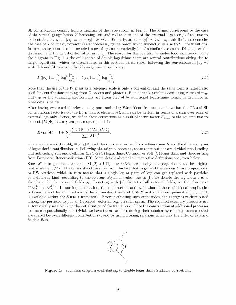
SL contributions coming from a diagram of the type shown in Fig. 1. The former correspond to the caseof the virtual gauge boson V becoming soft and collinear to one of the external legs i or j of the matrixelement M, i.e. when |rij | ≡ |pi + pj |2 � m2

W . Similarly, as |pi + pj |2 ∼ 2 pi · pj , this limit also encodesthe case of a collinear, non-soft (and vice-versa) gauge boson which instead gives rise to SL contributions.In turn, these must also be included, since they can numerically be of a similar size as the DL one, see thediscussion and the detailed derivation in [1, 5]. The reason for this can also be understood intuitively: whilethe diagram in Fig. 1 is the only source of double logarithms there are several contributions giving rise tosingle logarithms, which we discuss later in this section. In all cases, following the conventions in [1], wewrite DL and SL terms in the following way, respectively:

L (|rij |) ≡α

4πlog2 |rij |

m2W

, l (rij) ≡α

4πlog

rijm2W

. (2.1)

Note that the use of the W mass as a reference scale is only a convention and the same form is indeed alsoused for contributions coming from Z bosons and photons. Remainder logarithms containing ratios of mW

and mZ or the vanishing photon mass are taken care of by additional logarithmic terms, as explained inmore details below.

After having evaluated all relevant diagrams, and using Ward identities, one can show that the DL and SLcontributions factorise off the Born matrix element M, and can be written in terms of a sum over pairs ofexternal legs only. Hence, we define these corrections as a multiplicative factor KNLL to the squared matrixelement |M(Φ)|2 at a given phase space point Φ:

KNLL (Φ) = 1 +∑c

∑h 2 Re {(δcMh)M∗h}∑

h |Mh|2, (2.2)

where we have writtenMh ≡Mh(Φ) and the sums go over helicity configurations h and the different typesof logarithmic contributions c. Following the original notation, these contributions are divided into Leadingand Subleading Soft and Collinear (LSC/SSC) logarithms, Collinear or Soft (C) logarithms and those arisingfrom Parameter Renormalisation (PR). More details about their respective definitions are given below.

Since δc is in general a tensor in SU(2) × U(1), the δcMh are usually not proportional to the originalmatrix elementMh. The tensor structure come from the fact that in general the various δc are proportionalto EW vertices, which in turn means that a single leg or pairs of legs can get replaced with particlesof a different kind, according to the relevant Feynman rules. As in [1], we denote the leg index i as ashorthand for the external fields φi. Denoting with {i} the set of all external fields, we therefore have

δcM{i}h ∝ M{i′}

h . In our implementation, the construction and evaluation of these additional amplitudesis taken care of by an interface to the automated tree-level COMIX matrix element generator [13], whichis available within the SHERPA framework. Before evaluating such amplitudes, the energy is re-distributedamong the particles to put all (replaced) external legs on-shell again. The required auxiliary processes areautomatically set up during the initialisation of the framework. Since the construction of additional processescan be computationally non-trivial, we have taken care of reducing their number by re-using processes thatare shared between different contributions c, and by using crossing relations when only the order of externalfields differs.

M

i

j

V

Figure 1: Feynman diagram contributing to double-logarithmic Sudakov corrections.

3

In our implementation we consistently neglect purely electromagnetic logarithms which arise from the gapbetween zero (or the fictitious photon mass) and mW . In SHERPA such logarithms can be treated in either oftwo ways. First, one can compute the purely electromagnetic NLO correction to the desired process, consist-ing of both virtual and real photon emission, which gives the desired logarithm at fixed order. Alternatively,one can resum soft-photon emission to all orders, which in SHERPA is achieved through the formalism ofYennie, Frautschi and Suura (YFS) [33] or by a QED parton shower, as is discussed e.g. in [35]. In contrast,logarithms originating from the running between the W mass and the Z mass are included, as we explainin the next paragraphs, where we discuss the individual contributions δc.

Leading Soft-Collinear logarithms: LSC The leading corrections are given by the soft and collinear limitof a virtual gauge boson and are proportional to L(|rkl|). By writing

L (|rkl|) = L (s) + 2 l(s) log|rkl|s

+ L (|rkl| , s) , (2.3)

and neglecting the last term on the right-hand side, which is of order O(1), one has split the soft-collinearcontribution into a leading soft-collinear (LSC) and a angular-dependent subleading soft-collinear (SSC) one,corresponding to the first and second term on the right-hand side, respectively. The full LSC correction isthen given by

δLSCMi1...in =

n∑k=1

δLSCi′kik

(k)Mi1...i′k...in

0 , (2.4)

where the sum runs over the n external legs, and the coefficient matrix on the right-hand side is given by

δLSCi′kik

(k) = −1

2

[Cewi′kik

(k)L(s)− 2(IZ(k)

)2i′kik

logM2Z

M2W

l(s)

]= δLSC

i′kik(k) + δZi′kik

(k). (2.5)

Cew and IZ are the electroweak Casimir operator and the Z gauge coupling, respectively. The second termδZ appears as an artefact of writing L(s) and l(s) in terms of the W mass even for Z boson loops, andhence the inclusion of this term takes care of the gap between the Z and the W mass at NLL accuracy. Wedenote the remaining terms with the superscript “LSC”. Note that this term is in general non-diagonal,since Cew mixes photons and Z bosons. As is explicit in Eq. (2.2), coefficients need to be computed perhelicity configuration; in the case of longitudinally polarised vector boson appearing as external particles,they need to be replaced with the corresponding Goldstone bosons using the Goldstone Boson EquivalenceTheorem. This is a consequence of the scaling of longitudinal polarisation vectors with the mass of theparticle, which prevents the direct application of the eikonal approximation used to evaluate the high-energylimit, as is detailed in [1]. To calculate such matrix elements we have extended the default Standard Modelimplementation in SHERPA with a full Standard Model including Goldstone bosons generated through theUFO interface of SHERPA [36, 37]. We have tested this implementation thoroughly against RECOLA [38].‡

Subleading Soft-Collinear logarithms: SSC The second term in Eq. 2.3 gives rise to the angular-dependent subleading part of the corrections from soft-collinear gauge-boson loops. It can be written as asum over pairs of external particles:

δSSCMi1...in =

n∑k=1

∑l<k

∑Va=A,Z,W±

δVa,SSCi′kiki

′lil

(k, l)Mi1...i′k...i

′l...in

0 , (2.6)

where the coefficient matrices for the different gauge bosons Va = A,Z,W± are

δVa,SSCi′kiki

′lil

(k, l) = 2IVai′kik(k)I Vai′lil

(l) log|rkl|sl(s).

Note that while the photon couplings IA are diagonal, the eigenvalues for IZ and I± ≡ IW±

can be non-diagonal, leading again to replacements of external legs as described in the LSC case.

‡Note that in particular this adds the possibility for SHERPA users to compute Goldstone bosons contributions to any desiredprocess, independently of whether this is done in the context of calculating EW Sudakov corrections.

4

Collinear or soft single logarithms: C The two sources that provide either collinear or soft logarithmsare the running of the field renormalisation constants, and the collinear limit of the loop diagrams whereone external leg splits into two internal lines, one of which being a vector boson Va. The ensuing correctionfactor can be written as a sum over external legs:

δCMi1...in =

n∑k=1

δCi′kik

(k)Mi1...i′k...in

0 . (2.7)

For chiral fermions f , the coefficient matrix is given by

δCfσfσ′

(fκ) = δσσ′

[3

2Cewfκ −

1

8s2w

((1 + δκR)

m2fσ

M2W

+ δκL

m2f−σ

M2W

)]l(s) = δC

fσfσ′(fκ) + δYuk

fσfσ′(fκ) . (2.8)

We label the chirality of the fermion by κ, which can take either the value L (left-handed) or R (right-handed). The label σ specifies the isospin, its values ± refer to up-type quarks/neutrinos or down-typequarks/leptons, respectively. The sine (cosine) of the Weinberg angle is denoted by sw (cw). Note thatwe further subdivide the collinear contributions for fermion legs into “Yukawa” terms formed by termsproportional to the ratio of the fermion masses over the W mass, which we denote by the superscript “Yuk”,and the remaining collinear contributions denoted by the superscript “C”. These Yukawa terms only appear

for external fermions, such that for all other external particles ϕ, we have δCϕ′ϕ = δC

ϕ′ϕ. For charged andneutral transverse gauge bosons,

δCWσWσ′ (VT) = δσσ′

1

2bewW l(s) and δC

N ′N (VT) =1

2[EN ′Nb

ewAZ + bew

N ′N ] l(s) with E ≡(

0 1−1 0

)(2.9)

must be used, where the bew are combinations of Dynkin operators that are proportional to the one-loopcoefficients of the β-function for the running of the gauge-boson self-energies and mixing energies. Theirvalues are given in terms of sw and cw in [1].

Longitudinally polarised vector bosons are again replaced with Goldstone bosons. When using the matrixelement on the right-hand side of Eq. (2.7) in the physical EW phase, the following (diagonal) coefficientmatrices must be used for charged and neutral longitudinal gauge bosons:

δCWσWσ′ (VL)→ δC

φ±φ±(Φ) =

[2Cew

Φ −NC

4s2w

m2t

M2W

]l(s), (2.10)

δCN ′N (VT)→ δC

χχ(Φ) =

[2Cew

Φ −NC

4s2w

m2t

M2W

]l(s), (2.11)

where NC = 3 is the number of colour charges.

Parameter Renormalisation logarithms: PR The last contribution we consider is the one comingfrom the renormalisation of EW parameters, such as boson and fermion masses and the QED coupling α,and all derived quantities. The way we extract these terms, is by running all EW parameters up to a givenscale, µEW, which in all cases presented here corresponds to the partonic scattering centre of mass energy,and re-evaluate the matrix element value with these evolved parameters. We then take the ratio of this‘High Energy’ (HE) matrix element with respect to the original value, such that, calling {pew} the completeset of EW parameters,

δPRi1...in =

(Mi1...in

HE ({pew}(µEW))

Mi1...in({pew})− 1

)∼ 1

Mi1...in

∑p∈{pew}

δMi1...in

δpδp. (2.12)

The evolution of each EW parameter is obtained through

pew(µEW) = {pew}(

1 +δpew

pew

), (2.13)

5

and the exact expressions for δpew can be found in Eqs. (5.4–5.22) of [1].

The right hand side of Eq. (2.12) corresponds to the original derivation of Denner and Pozzorini, while theleft hand side is the actual implementation we have used. The two differ by terms that are formally of higherorder, (α logµ2

EW/m2W )2. In fact, although they are logarithmically enhanced, they are suppressed by an

additional power of α with respect to the leading terms considered here, α log2 µ2EW/m

2W .

Generating event samples with EW Sudakov logarithmic contributions After having discussedthe individual contributions c, we can return to Eq. (2.2), for which we now have all the ingredients toevaluate it for an event with the phase-space point Φ. Defining the relative logarithmic contributions ∆c,we can rewrite it as

KNLL (Φ) = 1 +∑c

∆c = 1 + ∆LSC + ∆Z + ∆SSC + ∆C + ∆Yuk + ∆PR. (2.14)

In the event sample, the relative contributions ∆c are given in the form of named HEPMC weights [14](details on the naming will be given in the manual of the upcoming SHERPA release). This is done to leavethe user freedom on how to combine such weights with the main event weight.

In the context of results, Sec. 3, we employ these corrections in either of two ways. One way is to includethem at fixed order,

dσLO + NLL (Φ) = dΦB (Φ) KNLL (Φ) , (2.15)

where B is the Born contribution. The alternative is to exploit the fact that Sudakov EW logarithmsexponentiate (see Refs. [22]–[31]) to construct a resummed fully differential cross section

dσLO + NLL (resum) (Φ) = dΦB (Φ) KresumNLL (Φ) = dΦB (Φ) e(1−KNLL(Φ)) , (2.16)

following the approach discussed in [32].

Matching to higher orders and parton showers SHERPA internally provides the possibility to the userto obtain NLO corrections, both of QCD [39] and EW [15] origin, and to further generate fully showered [40,41] and hadronised events [7]. In addition one is able to merge samples with higher multiplicities in QCDthrough the CKKW [42], or the MEPS@NLO [43] algorithms. In all of the above cases (except the NLO EW),the corrections implemented here can be simply applied using the K factor methods in SHERPA to one or allthe desired processes of the calculations, as there is no double counting between EW Sudakov corrections andpure QCD ones. A similar reasoning can be applied for the combination with a pure QCD parton shower.Although we do not report the result of this additional check here, we have tested the combination of theEW Sudakov corrections with the default shower of SHERPA. Technical checks and physics applications forthe combination with matching and merging schemes, and for the combination with QED logarithms, areleft for a future publication.

If one aims at matching Sudakov logarithms to higher-order EW effects, such as for example combining fixedorder NLO EW results with a resummed NLL Sudakov correction, it is for now required for the user tomanually do the subtraction of double counting that one encounters in these cases. An automation of sucha scheme is also outside the scope of this publication, and will be explored in the future.

3 Results

Before discussing our physics applications, we report a number of exact comparisons to other existing cal-culations of NLL EW Sudakov logarithms. A subset of the results used for this comparison for pp → V jprocesses is shown in App. A. They all agree with reference ones on a sub-percent level over the entire probedtransverse momentum range from pT,V = 100 GeV to 2000 GeV. In addition to this, the implementationhas been guided by passing a number of tests based on a direct comparison of tabulated numerical valuesfor each contribution discussed in Sec. 2 in the high-energy limit, that are given for several electron-positron

6

collision processes in [1] and for the pp → WZ and pp → Wγ processes in [44]. Our final implementationpasses all these tests.

In the remainder of this section, we present a selection of physics results obtained using our implementationand where possible show comparisons with existing alternative calculations. The aim is twofold, first wewish to show the variety of processes that can be computed with our implementation, and second we wantto compare to existing alternative methods to obtain EW corrections to further study the quality of theapproximation. In particular, where available, we compare our NLL predictions to full NLO EW corrections,as well as to the EWvirt approximation defined in [21]. It is important to note that we only consider EWcorrections to purely EW processes here, such that there are no subleading Born corrections that mightotherwise complicate the comparison to a full EW NLO calculation or to the EWvirt approximation. Weconsider diboson production, dijet production, and Z production in association with 4 jets. In all cases, wefocus on the discussion of (large) transverse momentum distributions, since they are directly sensitive to thegrowing effect of the logarithmic contributions when approaching the high-energy limit.

The logarithmic contributions are applied to parton-level LO calculations provided by the COMIX matrixelement generator implemented in SHERPA. The parton shower and non-perturbative parts of the simulationare disabled, including the simulation of multiple interactions and beam remnants, and the hadronisation.Also higher-order QED corrections to the matrix element and by YFS-type resummation are turned off.The contributions to the NLL corrections as defined in Sec. 2 are calculated individually and combined a-posteriori, such that we can study their effects both individually and combined. We consider the fixed-orderand the resummed option for the combination, as detailed in Eqs. (2.15) and (2.16), respectively.

For the analysis, we use the Rivet 2 [45] framework, and events are passed to analysis using the HEPMCevent record library. Unless otherwise specified, simulations are obtained using the NNPDF3.1, next-to-next-to-leading order PDF set [46], while in processes where we include photon initiated processes we insteaduse the NNPDF3.1 LUX PDF set [47]. In all cases, PDFs are obtained through the LHAPDF [48] interfaceimplemented in SHERPA. When jets appear in the final state, we cluster them using the anti-kT algorithm [49]with a jet radius parameter of R = 0.4, through an interface to FASTJET [50]. The CKM matrix in ourcalculation is equal to the unit matrix, i.e. no mixing of the quark generations is allowed. Electroweakparameters are determined using tree-level relations using a QED coupling value of α(mZ) = 1/128.802 andthe following set of masses and decay widths, if not explicitly mentioned otherwise:

mW = 80.385 GeV mZ = 91.1876 GeV mh = 125 GeV

ΓW = 2.085 GeV ΓZ = 2.4952 GeV Γh = 0.004 07 GeV.

Note that α is not running in the nominal calculation as running effects are all accounted for by the PRcontributions.

3.1 WW production in pp collisions at 13 and 100 TeV

Our first application is the calculation of EW Sudakov effects in on-shell W boson pair production at hadroncolliders, which has lately been experimentally probed at the LHC [51, 52], e.g. to search for anomalousgauge couplings. We compare the Sudakov EW approximation to both the full NLO EW calculation and theEWvirt approximation. The latter has been applied to WW production in [35, 53]. In addition to that, EWcorrections for WW production have also been studied in [54, 55, 56, 57, 58, 59], and NNLL EW Sudakovcorrections have been calculated in [54].

We have performed this study at current LHC energies,√s = 13 TeV, as well as at a possible future hadron

collider with√s = 100 TeV. In all cases, we include photon induced channels (they can be sizeable at large

energies [55]), and we set the renormalisation and factorisation scales to µ2R,F = 1

2 (2m2W +

∑i p

2T,i), where

the sum runs over the final-state W bosons, following the choice for gauge-boson pair production in [60].Lastly, we set the widths of the Z and W boson consistently to 0, as the W is kept on-shell in the matrixelements.

In Fig. 2 we report results for the transverse momentum of each W boson in the final state for bothcentre of mass energies. Plots are divided into four panels, of which the first one collects results for thevarious predictions. The second and third panels report the ratio to the leading order and to the EWvirt

7

pWT [GeV]

10−7

10−5

10−3

10−1

101

dσ/dpT

[pb

/G

eV]

Sherpa + OpenLoopspp→WW√s = 13 TeV

LO

LO+NLL

LO+NLL (resum)

NLO EWNLO EWvirt

NLO EW (jet veto)

pWT [GeV]

0.2

0.4

0.6

0.8

1.0

1.2

rati

oto

LO

pWT [GeV]

0.8

1.0

1.2

rati

oto

EW

vir

t

102

103

pT,W [GeV]

0.2

0.4

0.6

0.8

1.0

1.2

LO

+N

LL

contr

ibL

O

individual NLL contributionsC

LSC

PR

SSC

Yuk

Z

pWT [GeV]

10−7

10−5

10−3

10−1

101

dσ/dpT

[pb

/G

eV]

Sherpa + OpenLoopspp→WW√

s = 100 TeV

LO

LO+NLL

LO+NLL (resum)

NLO EWNLO EWvirt

NLO EW (jet veto)

pWT [GeV]

0.2

0.4

0.6

0.8

1.0

1.2

rati

oto

LO

pWT [GeV]

0.8

1.0

1.2ra

tio

toE

Wvir

t

102

103

pT,W [GeV]

0.2

0.4

0.6

0.8

1.0

1.2

LO

+N

LL

contr

ibL

O

individual NLL contributionsC

LSC

PR

SSC

Yuk

Z

Figure 2: The transverse momentum of the individual W bosons in W boson pair production from proton-proton collisions (including photon induced channels) at

√s = 13 TeV (left) and 100 TeV (right).

The baseline LO and NLO EW calculations are compared with the results of the LO+NLL cal-culation and its variant, where the logarithmic corrections are resummed (“LO+NLL (resum)”).In addition, the virtual approximation EWvirt and a variant of the NLO EW calculation withadditional jets vetoed are also included. The ratio plots show the ratios to the LO and to theEWvirt calculation, and the relative size of each NLL contribution.

approximation, respectively. The aim is to show the general behaviour of EW corrections in the tail ofdistributions in the former, while the latter serves as a direct comparison between the Sudakov and theEWvirt approximations. Finally the fourth panel shows the relative impact of the individual contributions∆c appearing in Eq. (2.14).

Looking at the second panel, we see that all but the full NLO EW calculation show a strong suppression inthe pT > mW region, reaching between −70 % and −90 % at pT = 2 TeV. This effect is the main effect we

8

discuss in this work, and it is referred to as Sudakov suppression. To explicitly confirm that this behaviouroriginates from virtual contributions of EW nature, we compare the Sudakov LO+NLL curve to the NLOEW and EWvirt approximations. Indeed, the latter only takes into account virtual corrections and theminimal amount of integrated counter terms to render the cross section finite. The Sudakov approximationis close to that for both centre of mass energies (see also the third panel), with deviations of the order ofa few percent. It begins to deviate more at the end of the spectrum, with similar behaviours observed forboth collider setups. However, with a Sudakov suppression of 70 % and more, we are already in a regimewhere the relative corrections become O(1) and a fixed logarithmic order description becomes invalid. Infact, at pT,W & 3 TeV, the LO+NLL becomes negative both at

√s = 13 TeV and 100 TeV, the same being

true for the EWvirt approximation. Note in particular, that this is the main reason for choosing to show thepT distribution only up to pT = 2 TeV in Fig. 2 for both collider setups.

It is also clear from the second panel that for both setups, the full NLO EW calculation does not showsuch large suppressions, and in the context of the question whether to use EW Sudakovs or the EWvirt toapproximate the full corrections, this may be worrisome. However, in the full calculation we have includedthe real emission matrix elements, which also show a logarithmic enhancement at high pT , as e.g. discussedin [56]. In this case, the real emission contribution almost entirely cancels the Sudakov suppression at√s = 13 TeV, and even overcompensates it by about 20 % in the pT,W . 1 TeV region for

√s = 100 TeV. To

show that this is the case, we have also reported a jet-vetoed NLO EW simulation, which indeed again showsthe high pT suppression as expected. Moreover, we have included a prediction labelled “LO+NLL (resum)”,where we exponentiate the Sudakov contribution using Eq. (2.16). It is similar to the NLL approximation,but resumming these logarithms leads to a smaller suppression in the large pT tail, which is reduced by about20 % at pT = 2 TeV, thus increasing the range of validity compared to the non-exponentiated prediction.Moreover, this agrees well qualitatively with the NNLL result reported in [54], and suggests that evenhigher-order logarithmic effects should be rather small in comparison in the considered observable range.

Lastly, we compare the individual LL and NLL contributions. As expected, we find that the double logarith-mic LSC term is the largest contribution and drives the Sudakov suppression. Some single logarithmic terms,in particular the C terms, also give a sizeable contribution, reducing the net suppression. This confirms thatthe inclusion of single logarithmic terms is needed in order to provide accurate predictions in the Sudakovapproximation, with deviations of the order of O(10 %) with respect to the EWvirt calculation. Comparingthe individual contributions for the two collider energies, we see qualitatively similar effects. As can beexpected from a larger admixture of bb initial states, the ∆Yuk is enhanced at the larger collider energy.

3.2 EW-induced dijet production in pp collisions at 13 TeV

For the second comparison in this section, we simulate purely EW dijet production in hadronic collisions at√s = 13 TeV at the Born-level perturbative order O(α2α0

s). As for the case of diboson production we addphoton initiated channels, and we also include photons in the set of final-state partons, such that γγ and γjproduction is also part of our sample. Partons are thus clustered into jets which are then sorted by their pT .We select events requiring at least two jets, the leading jet (in pT ) to have a pT > 60 GeV and the subleadingjet to have a pT > 30 GeV. Note in particular that for all but the real emission case in the full NLO EWsimulation, this corresponds to imposing a pT cut on the two generated partons. The renormalisation andfactorisation scales are set to µ2

R,F = H2T = (

∑i pT,i)

2, where the sum runs over final-state partons.

We compare our LO+NLL EW results, as in the previous subsection, with the LO, the NLO EW and theEWvirt predictions. NLO EW corrections for dijet production have been first discussed in [61, 62], while [63]discusses those corrections in the context of the 3-to-2-jet ratio R32. In this context, we only consider EWcorrections to the Born process described above, i.e. we consider the O(α0

sα3) contributions, which is a subset

of the contributions considered in the above references.

In Fig. 3 (left), we present the transverse momentum distribution of the leading jet pT given by the LO+NLLEW calculation, again both at fixed order and resummed, see Eqs. (2.15) and (2.16). As for W pairproduction, the plot is divided into four panels. However, this time we do not include jet-vetoed NLOresults, as in this case we do not observe large real emission contributions. The panels below the main plotgive the ratio to the LO calculation, the ratio to the EWvirt approximation, and the ratio of each NLLcontribution to the LO calculation.

9

Compared to W pair production, we observe a smaller but still sizeable Sudakov suppression, reachingapproximately −40 % at pT = 2 TeV. The NLO contributions not included in the NLO EWvirt (i.e. mainlyreal emission terms) are small and cancel the Sudakov suppression only by a few percent and as such boththe Sudakov and the EWvirt approximations agree well throughout the pT spectrum with the full NLOcalculation. The same is true for the resummed NLL case which gives a Sudakov suppression of −30 % forpT = 2 TeV. Note that a small step can be seen for pT ∼ mW in the Sudakov approximation. The reasonfor this is that we force, during the simulation, all Sudakov contributions to be zero when at least one ofthe invariants formed by the scalar product of the external momenta is below the W mass, as Sudakovcorrections are technically only valid in the high-energy limit. This threshold behaviour can be disabled,giving a smoother transition between the LO and the LO+NLL, as can be seen for example in Fig. 2.

Comparing the individual NLL contributions we find again that the double logarithmic LSC term is thelargest contribution, its size is however reduced by a third compared to the diboson case, since the prefactorCew in Eq. (2.5) is smaller for quarks and photons compared to W bosons. Among the single logarithmicterms the C and PR terms are the most sizeable over the whole range, and are of a similar size compared tothe diboson case, while the SSC contribution only give a small contribution. Again, subleading terms mustbe included to approximate the NLO calculation at the observed 10 % level, although we observe an almostentire accidental cancellation, in this case, of the SL terms.

3.3 Off-shell Z production in association with 4 jets in pp collisions at 13 TeV

As a final example, we present for the first time the LO+NLL calculation for e+e− production in associationwith four additional jets from proton-proton collisions at

√s = 13 TeV. The process is one of the key

benchmark processes at the LHC to make precision tests of perturbative QCD and is a prominent backgroundconstituent for several Standard Model and New Physics processes. In this case, we neglect photon inducedcontributions, to better compare to the NLL effects in Z plus one-jet production presented in App. A,which in turn is set up as a direct comparison to [8]. For the same reason, in this case, we only considerQCD partons in the final state. The factorisation and renormalisation scale are set to µ2

F = µ2R = H ′2T =

(MT,`` +∑i pT,i)

2/4.0, where MT,`` is the transverse mass of the electron-positron pair and the sum runsover the final-state partons. This choice is inspired by [64], where the full next-to-leading QCD calculationis presented.

As we consider here an off-shell Z, the invariant mass formed by its decay products is on average onlyslightly above the W mass threshold. This may cause an issue as this is one of the invariants considered inthe definition of the high-energy limit discussed in Sec. 2, and therefore this limit is strictly speaking notfulfilled. In turn, this can introduce sizeable logarithms in particular in Eq. (2.6). However, in practice weonly see a small number of large K factors, that only contribute a negligible fraction of the overall crosssection. For set-ups at a larger centre of mass energy, one should monitor this behaviour closely, as theaverage value of s in Eq. (2.6) would increase too. We therefore foresee that a more careful treatment mightbe required then, e.g. by vetoing EW Sudakov K factors whenever |rkl| � s.

In Fig. 3 (right), we present the LO+NLL EW calculation of the transverse momentum distribution of thereconstructed Z boson. To our knowledge, there is no existing NLO EW calculation to compare it against§,hence we do not have a ratio-to-NLO plot in this case. However, we do show the ratio-to-NLL plot and theplot that shows the different contributions of the LO+NLL calculation, as for the other processes.

The sizeable error bands give the MC errors of the LO calculation. Note that the errors of the LO and theLO+NLL calculation are fully correlated, since the NLL terms are completely determined by the phase-spacepoint of the LO event, and the same LO event samples are used for both predictions. Hence the reportedratios are in fact very precise. With the aim of additionally making a comparison to the Z+j result reportedin Fig. 4 (right panel), we opt for a linear x axis, in contrast with the other results of this section. In bothcases we see a similar overall LO+NLL effect, reaching approximately −40 % for pT . 2 TeV. This in turnimplies that the effects of considering an off-shell Z (as opposed to an on-shell decay) as well as the additionalnumber of jets have very little effect on the size of the Sudakov corrections. Finding similar EW correctionsfor processes that only differ in their number of additional QCD emissions can be explained by the fact that

§Note that while such a calculation has not yet been published, existing tools, including SHERPA in conjunction withOpenLoops [65], are in principle able to produce such a set-up.

10

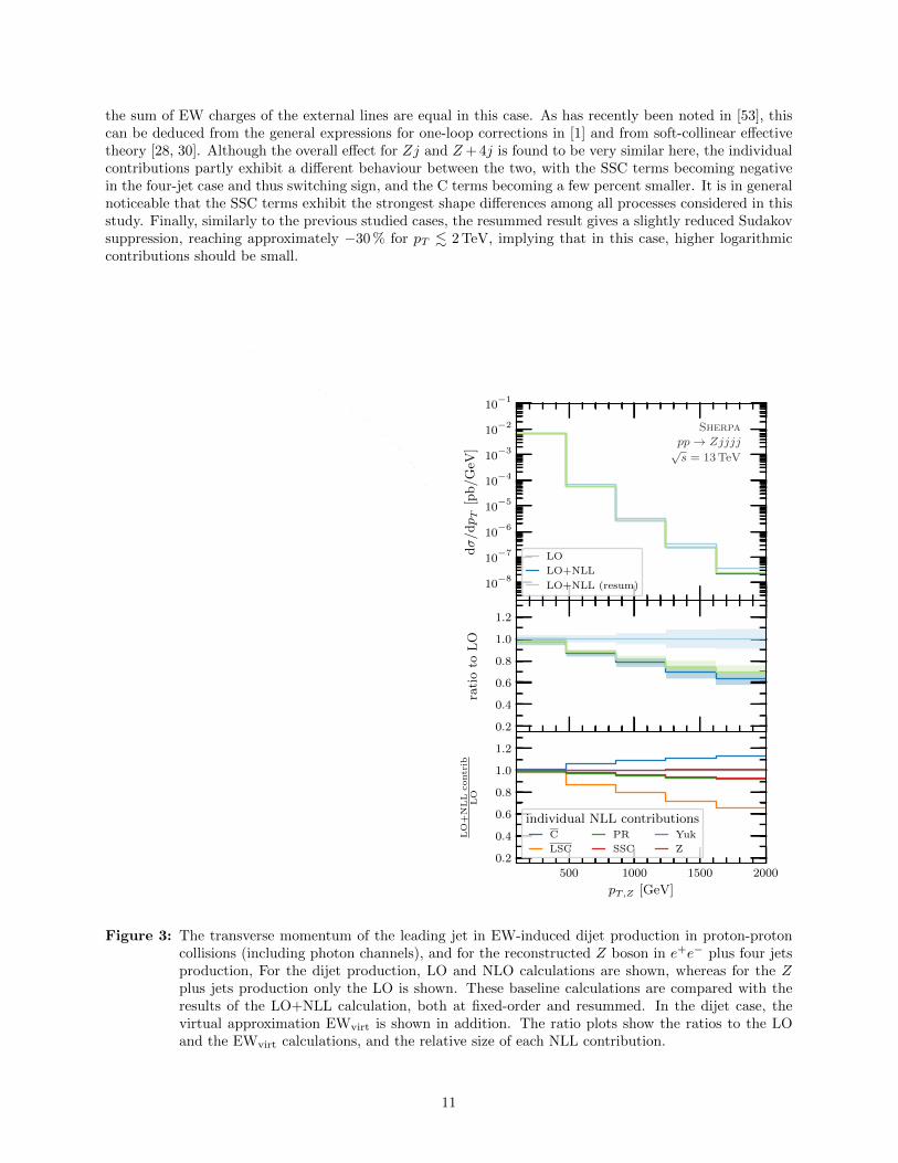
the sum of EW charges of the external lines are equal in this case. As has recently been noted in [53], thiscan be deduced from the general expressions for one-loop corrections in [1] and from soft-collinear effectivetheory [28, 30]. Although the overall effect for Zj and Z+ 4j is found to be very similar here, the individualcontributions partly exhibit a different behaviour between the two, with the SSC terms becoming negativein the four-jet case and thus switching sign, and the C terms becoming a few percent smaller. It is in generalnoticeable that the SSC terms exhibit the strongest shape differences among all processes considered in thisstudy. Finally, similarly to the previous studied cases, the resummed result gives a slightly reduced Sudakovsuppression, reaching approximately −30 % for pT . 2 TeV, implying that in this case, higher logarithmiccontributions should be small.

pT (jet 1) [GeV]

10−7

10−5

10−3

10−1

101

103

dσ/dpT

[pb

/G

eV]

Sherpa + OpenLoops

EW-induced pp→ jj/jγ/γγ√s = 13 TeV

LO

LO+NLL

LO+NLL (resum)

NLO EWNLO EWvirt

pT (jet 1) [GeV]

0.2

0.4

0.6

0.8

1.0

1.2

rati

oto

LO

pT (jet 1) [GeV]

0.8

1.0

1.2

rati

oto

EW

vir

t

102

103

pleadT,j [GeV]

0.2

0.4

0.6

0.8

1.0

1.2

LO

+N

LL

contr

ibL

O

individual NLL contributionsC

LSC

PR

SSC

Yuk

Z

pZT [GeV]

10−8

10−7

10−6

10−5

10−4

10−3

10−2

10−1

dσ/dpT

[pb/G

eV]

Sherpapp→ Zjjjj√s = 13 TeV

LO

LO+NLL

LO+NLL (resum)

pZT [GeV]

0.2

0.4

0.6

0.8

1.0

1.2

rati

oto

LO

500 1000 1500 2000

pT,Z [GeV]

0.2

0.4

0.6

0.8

1.0

1.2

LO

+N

LL

contr

ibL

O

individual NLL contributionsC

LSC

PR

SSC

Yuk

Z

Figure 3: The transverse momentum of the leading jet in EW-induced dijet production in proton-protoncollisions (including photon channels), and for the reconstructed Z boson in e+e− plus four jetsproduction, For the dijet production, LO and NLO calculations are shown, whereas for the Zplus jets production only the LO is shown. These baseline calculations are compared with theresults of the LO+NLL calculation, both at fixed-order and resummed. In the dijet case, thevirtual approximation EWvirt is shown in addition. The ratio plots show the ratios to the LOand the EWvirt calculations, and the relative size of each NLL contribution.

11

4 Conclusions

We have presented for the first time a complete, automatic and fully general implementation of the algorithmpresented in [1] to compute double and single logarithmic contributions of one-loop EW corrections, dubbedas EW Sudakov logarithms. These corrections can give rise to large shape distortions in the high-energytail of distributions, and are therefore an important contribution in order to improve the accuracy of theprediction in this region. Sudakov logarithms can provide a good approximation of the full next-to-leadingEW corrections. An exponentiation of the corrections can be used to resum the logarithmic effects andextend the region of validity of the approximation.

In our implementation, each term contributing to the Sudakov approximation is returned to the user inthe form of an additional weight, such that the user can study them individually, add their sum to thenominal event weight, or exponentiate them first. Our implementation will be made available with the nextupcoming major release of the SHERPA Monte Carlo event generator. We have tested our implementationagainst an array of existing results in the same approximation, and for a variety of processes against fullNLO EW corrections and the virtual approximation EWvirt, which is also available in SHERPA. A selectionof such tests is reported in this work, where we see that indeed EW Sudakov logarithms give rise to largecontributions and model the full NLO corrections well when real emissions are small. We stress that ourimplementation is not limited to the examples shown here, but it automatically computes such corrections forany Standard Model process. In terms of final-state multiplicity it is only limited by the available computingresources.

In a future publication we plan to apply the new implementation in the context of state-of-the-art eventgeneration methods, in particular to combine them with the matching and merging of higher-order QCDcorrections and the QCD parton shower, while also taking into account logarithmic QED corrections usingthe YFS or QED parton shower implementation in SHERPA. This will allow for an automated use of themethod for the generation of event samples in any LHC or future collider context, in the form of optionaladditive weights. As discussed towards the end of Sec. 2, we foresee that this is a straightforward exercise,since there is no double counting among the different corrections, and applying differential K factors correctlywithin these methods is already established within the SHERPA framework. The result should also allow forthe inclusion of subleading Born contributions, as the EWvirt scheme in SHERPA does. The automatedcombination of (exponentiated) EW Sudakov logarithms with fixed-order NLO EW corrections is anotherpossible follow-up, given the presence of phenomenologically relevant applications.

Acknowledgements

We wish to thank Stefano Pozzorini for the help provided at various stages with respect to his originalwork, as well as Marek Schonherr, Steffen Schumann, Stefan Hoche and Frank Krauss and all our SHERPA

colleagues for stimulating discussions, technical help and comments on the draft. We also thank JenniferThompson for the collaboration in the early stage of this work. The work of DN is supported by the ERCStarting Grant 714788 REINVENT.

12

A Validation plots for V plus jet production in pp collisions at 13 TeV

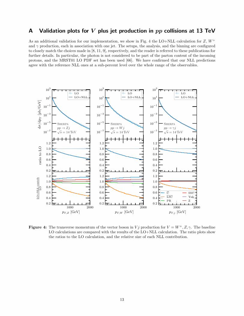
As an additional validation for our implementation, we show in Fig. 4 the LO+NLL calculation for Z, W+

and γ production, each in association with one jet. The setups, the analysis, and the binning are configuredto closely match the choices made in [8, 11, 9], respectively, and the reader is referred to these publications forfurther details. In particular, the photon is not considered to be part of the parton content of the incomingprotons, and the MRST01 LO PDF set has been used [66]. We have confirmed that our NLL predictionsagree with the reference NLL ones at a sub-percent level over the whole range of the observables.

pZT [GeV]

10−7

10−5

10−3

10−1

101

103

dσ/dpT

[pb/G

eV]

Sherpapp→ Zj√s = 14 TeV

LO

LO+NLL

pZT [GeV]

0.2

0.4

0.6

0.8

1.0

1.2

rati

oto

LO

1000 2000

pT,Z [GeV]

0.2

0.4

0.6

0.8

1.0

1.2

LO

+N

LL

contr

ibL

O

10−7

10−5

10−3

10−1

101

103

Sherpapp→Wj√s = 14 TeV

LO

LO+NLL

0.2

0.4

0.6

0.8

1.0

1.2

1000 2000

pT,W [GeV]

0.2

0.4

0.6

0.8

1.0

1.2

10−7

10−5

10−3

10−1

101

103

Sherpapp→ γj√s = 14 TeV

LO

LO+NLL

0.2

0.4

0.6

0.8

1.0

1.2

1000 2000

pT,j [GeV]

0.2

0.4

0.6

0.8

1.0

1.2

C

LSC

PR

SSC

Yuk

Z

Figure 4: The transverse momentum of the vector boson in V j production for V = W+, Z, γ. The baselineLO calculations are compared with the results of the LO+NLL calculation. The ratio plots showthe ratios to the LO calculation, and the relative size of each NLL contribution.

13

References

[1] A. Denner and S. Pozzorini, One loop leading logarithms in electroweak radiative corrections. 1. Results,Eur.Phys.J. C18 (2001), 461–480, [arXiv:hep-ph/0010201 [hep-ph]].

[2] K. Mishra et al., Electroweak Corrections at High Energies, Community Summer Study 2013: Snowmasson the Mississippi, 8 2013.

[3] V. V. Sudakov, Vertex parts at very high-energies in quantum electrodynamics, Sov. Phys. JETP 3(1956), 65–71.

[4] A. Denner, M. Melles and S. Pozzorini, Two loop electroweak corrections at high-energies,Nucl.Phys.Proc.Suppl. 116 (2003), 18–22, [arXiv:hep-ph/0211196 [hep-ph]].

[5] A. Denner and S. Pozzorini, One loop leading logarithms in electroweak radiative corrections. 2. Factor-ization of collinear singularities, Eur.Phys.J. C21 (2001), 63–79, [arXiv:hep-ph/0104127 [hep-ph]].

[6] A. Denner and S. Pozzorini, An Algorithm for the high-energy expansion of multi-loop diagrams tonext-to-leading logarithmic accuracy, Nucl. Phys. B 717 (2005), 48–85, [hep-ph/0408068].

[7] E. Bothmann et al., Event Generation with Sherpa 2.2, SciPost Phys. 7 (2019), no. 3, 034,[arXiv:1905.09127 [hep-ph]].

[8] J. H. Khn, A. Kulesza, S. Pozzorini and M. Schulze, Logarithmic electroweak corrections to hadronic Z+1jet production at large transverse momentum, Phys. Lett. B 609 (2005), 277–285, [hep-ph/0408308].

[9] J. H. Khn, A. Kulesza, S. Pozzorini and M. Schulze, Electroweak corrections to hadronic photon pro-duction at large transverse momenta, JHEP 03 (2006), 059, [hep-ph/0508253].

[10] E. Accomando, A. Denner and S. Pozzorini, Logarithmic electroweak corrections to e+e− → νeνeW+W−,

JHEP 03 (2007), 078, [hep-ph/0611289].

[11] J. H. Khn, A. Kulesza, S. Pozzorini and M. Schulze, Electroweak corrections to hadronic production ofW bosons at large transverse momenta, Nucl. Phys. B 797 (2008), 27–77, [arXiv:0708.0476 [hep-ph]].

[12] M. Chiesa, G. Montagna, L. Barze, M. Moretti, O. Nicrosini, F. Piccinini and F. Tramontano, Elec-troweak Sudakov Corrections to New Physics Searches at the LHC, Phys. Rev. Lett. 111 (2013), no. 12,121801, [arXiv:1305.6837 [hep-ph]].

[13] T. Gleisberg and S. Hoche, Comix, a new matrix element generator, JHEP 12 (2008), 039,[arXiv:0808.3674 [hep-ph]].

[14] M. Dobbs and J. B. Hansen, The HepMC C++ Monte Carlo event record for High Energy Physics,Comput. Phys. Commun. 134 (2001), 41–46.

[15] M. Schonherr, An automated subtraction of NLO EW infrared divergences, Eur. Phys. J. C78 (2018),no. 2, 119, [arXiv:1712.07975 [hep-ph]].

[16] R. Frederix, S. Frixione, V. Hirschi, D. Pagani, H. S. Shao and M. Zaro, The automation of next-to-leading order electroweak calculations, JHEP 07 (2018), 185, [arXiv:1804.10017 [hep-ph]].

[17] S. Alioli, P. Nason, C. Oleari and E. Re, A general framework for implementing NLO calculations inshower Monte Carlo programs: the POWHEG BOX, JHEP 06 (2010), 043, [arXiv:1002.2581 [hep-ph]].

[18] B. Jager and G. Zanderighi, NLO corrections to electroweak and QCD production of W+W+ plus twojets in the POWHEGBOX, JHEP 11 (2011), 055, [arXiv:1108.0864 [hep-ph]].

[19] C. Bernaciak and D. Wackeroth, Combining NLO QCD and Electroweak Radiative Corrections to Wboson Production at Hadron Colliders in the POWHEG Framework, Phys.Rev. D85 (2012), 093003,[arXiv:1201.4804 [hep-ph]].

14

[20] L. Barze, G. Montagna, P. Nason, O. Nicrosini and F. Piccinini, Implementation of electroweak correc-tions in the POWHEG BOX: single W production, JHEP 04 (2012), 037, [arXiv:1202.0465 [hep-ph]],31 pages, 7 figures. Minor corrections, references added and updated. Final version to appear in JHEP.

[21] S. Kallweit, J. M. Lindert, P. Maierhofer, S. Pozzorini and M. Schonherr, NLO QCD+EW predic-tions for V + jets including off-shell vector-boson decays and multijet merging, JHEP 04 (2016), 021,[arXiv:1511.08692 [hep-ph]].

[22] V. S. Fadin, L. Lipatov, A. D. Martin and M. Melles, Resummation of double logarithms in electroweakhigh-energy processes, Phys. Rev. D 61 (2000), 094002, [hep-ph/9910338].

[23] M. Melles, Electroweak radiative corrections in high-energy processes, Phys. Rept. 375 (2003), 219–326,[hep-ph/0104232].

[24] M. Melles, Resummation of angular dependent corrections in spontaneously broken gauge theories, Eur.Phys. J. C 24 (2002), 193–204, [hep-ph/0108221].

[25] B. Jantzen, J. H. Khn, A. A. Penin and V. A. Smirnov, Two-loop electroweak logarithms, Phys. Rev. D72 (2005), 051301, [hep-ph/0504111], [Erratum: Phys.Rev.D 74, 019901 (2006)].

[26] J.-y. Chiu, F. Golf, R. Kelley and A. V. Manohar, Electroweak Sudakov corrections using effective fieldtheory, Phys. Rev. Lett. 100 (2008), 021802, [arXiv:0709.2377 [hep-ph]].

[27] J.-y. Chiu, F. Golf, R. Kelley and A. V. Manohar, Electroweak Corrections in High Energy Processesusing Effective Field Theory, Phys. Rev. D 77 (2008), 053004, [arXiv:0712.0396 [hep-ph]].

[28] J.-y. Chiu, R. Kelley and A. V. Manohar, Electroweak Corrections using Effective Field Theory: Appli-cations to the LHC, Phys. Rev. D 78 (2008), 073006, [arXiv:0806.1240 [hep-ph]].

[29] J.-y. Chiu, A. Fuhrer, R. Kelley and A. V. Manohar, Factorization Structure of Gauge Theory Am-plitudes and Application to Hard Scattering Processes at the LHC, Phys. Rev. D 80 (2009), 094013,[arXiv:0909.0012 [hep-ph]].

[30] J.-y. Chiu, A. Fuhrer, R. Kelley and A. V. Manohar, Soft and Collinear Functions for the StandardModel, Phys. Rev. D 81 (2010), 014023, [arXiv:0909.0947 [hep-ph]].

[31] A. Fuhrer, A. V. Manohar, J.-y. Chiu and R. Kelley, Radiative Corrections to Longitudinal and Trans-verse Gauge Boson and Higgs Production, Phys. Rev. D 81 (2010), 093005, [arXiv:1003.0025 [hep-ph]].

[32] J. Lindert et al., Precise predictions for V+ jets dark matter backgrounds, Eur. Phys. J. C 77 (2017),no. 12, 829, [arXiv:1705.04664 [hep-ph]].

[33] D. R. Yennie, S. C. Frautschi and H. Suura, The Infrared Divergence Phenomena and High-EnergyProcesses, Ann. Phys. 13 (1961), 379–452.

[34] A. Manohar, B. Shotwell, C. Bauer and S. Turczyk, Non-cancellation of electroweak logarithms in high-energy scattering, Phys. Lett. B 740 (2015), 179–187, [arXiv:1409.1918 [hep-ph]].

[35] S. Kallweit, J. M. Lindert, S. Pozzorini and M. Schonherr, NLO QCD+EW predictions for 2`2ν dibosonsignatures at the LHC, JHEP 11 (2017), 120, [arXiv:1705.00598 [hep-ph]].

[36] C. Degrande, C. Duhr, B. Fuks, D. Grellscheid, O. Mattelaer and T. Reiter, UFO - The UniversalFeynRules Output, Comput.Phys.Commun. 183 (2012), 1201–1214, [arXiv:1108.2040 [hep-ph]].

[37] S. Hoche, S. Kuttimalai, S. Schumann and F. Siegert, Beyond Standard Model calculations with Sherpa,Eur. Phys. J. C75 (2015), no. 3, 135, [arXiv:1412.6478 [hep-ph]].

[38] S. Actis, A. Denner, L. Hofer, A. Scharf and S. Uccirati, Automatizing one-loop computation in the SMwith RECOLA, PoS LL2014 (2014), 023.

15

[39] T. Gleisberg and F. Krauss, Automating dipole subtraction for QCD NLO calculations, Eur. Phys. J.C53 (2008), 501–523, [arXiv:0709.2881 [hep-ph]].

[40] S. Schumann and F. Krauss, A parton shower algorithm based on Catani-Seymour dipole factorisation,JHEP 03 (2008), 038, [arXiv:0709.1027 [hep-ph]].

[41] S. Hoche and S. Prestel, The midpoint between dipole and parton showers, Eur. Phys. J. C75 (2015),no. 9, 461, [arXiv:1506.05057 [hep-ph]].

[42] S. Catani, F. Krauss, R. Kuhn and B. R. Webber, QCD matrix elements + parton showers, JHEP 11(2001), 063, [hep-ph/0109231].

[43] S. Hoche, F. Krauss, M. Schonherr and F. Siegert, QCD matrix elements + parton showers: The NLOcase, JHEP 04 (2013), 027, [arXiv:1207.5030 [hep-ph]].

[44] S. Pozzorini, Electroweak radiative corrections at high-energies, Phd thesis, 2001.

[45] A. Buckley, J. Butterworth, L. Lonnblad, D. Grellscheid, H. Hoeth et al., Rivet user manual, Com-put.Phys.Commun. 184 (2013), 2803–2819, [arXiv:1003.0694 [hep-ph]].

[46] R. D. Ball et al., The NNPDF collaboration, Parton distributions from high-precision collider data, Eur.Phys. J. C 77 (2017), no. 10, 663, [arXiv:1706.00428 [hep-ph]].

[47] V. Bertone, S. Carrazza, N. P. Hartland and J. Rojo, The NNPDF collaboration, Illuminating thephoton content of the proton within a global PDF analysis, SciPost Phys. 5 (2018), no. 1, 008,[arXiv:1712.07053 [hep-ph]].

[48] A. Buckley, J. Ferrando, S. Lloyd, K. Nordstrom, B. Page, M. Rufenacht, M. Schonherr andG. Watt, LHAPDF6: parton density access in the LHC precision era, Eur. Phys. J. C75 (2015), 132,[arXiv:1412.7420 [hep-ph]].

[49] M. Cacciari, G. P. Salam and G. Soyez, The Anti-k(t) jet clustering algorithm, JHEP 04 (2008), 063,[arXiv:0802.1189 [hep-ph]].

[50] M. Cacciari, G. P. Salam and G. Soyez, FastJet user manual, Eur.Phys.J. C72 (2012), 1896,[arXiv:1111.6097 [hep-ph]].

[51] A. M. Sirunyan et al., The CMS collaboration, Search for anomalous couplings in boosted WW/WZ→`νqq production in proton-proton collisions at

√s = 8 TeV, Phys. Lett. B 772 (2017), 21–42,

[arXiv:1703.06095 [hep-ex]].

[52] M. Aaboud et al., The ATLAS collaboration, Measurement of fiducial and differential W+W− produc-tion cross-sections at

√s =13 TeV with the ATLAS detector, arXiv:1905.04242 [hep-ex].

[53] S. Brauer, A. Denner, M. Pellen, M. Schonherr and S. Schumann, Fixed-order and merged parton-shower predictions for WW and WWj production at the LHC including NLO QCD and EW corrections,arXiv:2005.12128 [hep-ph].

[54] J. Khn, F. Metzler, A. Penin and S. Uccirati, Next-to-Next-to-Leading Electroweak Logarithms for W-Pair Production at LHC, JHEP 06 (2011), 143, [arXiv:1101.2563 [hep-ph]].

[55] A. Bierweiler, T. Kasprzik, J. H. Khn and S. Uccirati, Electroweak corrections to W-boson pair produc-tion at the LHC, JHEP 11 (2012), 093, [arXiv:1208.3147 [hep-ph]].

[56] J. Baglio, L. D. Ninh and M. M. Weber, Massive gauge boson pair production at the LHC: a next-to-leading order story, Phys. Rev. D 88 (2013), 113005, [arXiv:1307.4331 [hep-ph]], [Erratum:Phys.Rev.D 94, 099902 (2016)].

[57] S. Gieseke, T. Kasprzik and J. H. Khn, Vector-boson pair production and electroweak corrections inHERWIG++, Eur. Phys. J. C 74 (2014), no. 8, 2988, [arXiv:1401.3964 [hep-ph]].

16

[58] W.-H. Li, R.-Y. Zhang, W.-G. Ma, L. Guo, X.-Z. Li and Y. Zhang, NLO QCD and electroweak correc-tions to WW+jet production with leptonic W -boson decays at LHC, Phys. Rev. D 92 (2015), no. 3,033005, [arXiv:1507.07332 [hep-ph]].

[59] B. Biedermann, M. Billoni, A. Denner, S. Dittmaier, L. Hofer, B. Jger and L. Salfelder, Next-to-leading-order electroweak corrections to pp → W+W− → 4 leptons at the LHC, JHEP 06 (2016), 065,[arXiv:1605.03419 [hep-ph]].

[60] E. Accomando, A. Denner and S. Pozzorini, Electroweak correction effects in gauge boson pair productionat the CERN LHC, Phys. Rev. D 65 (2002), 073003, [hep-ph/0110114].

[61] S. Dittmaier, A. Huss and C. Speckner, Weak radiative corrections to dijet production at hadron colliders,JHEP 11 (2012), 095, [arXiv:1210.0438 [hep-ph]].

[62] R. Frederix, S. Frixione, V. Hirschi, D. Pagani, H.-S. Shao and M. Zaro, The complete NLO correctionsto dijet hadroproduction, JHEP 04 (2017), 076, [arXiv:1612.06548 [hep-ph]].

[63] M. Reyer, M. Schonherr and S. Schumann, Full NLO corrections to 3-jet production and R32 at theLHC, Eur. Phys. J. C79 (2019), no. 4, 321, [arXiv:1902.01763 [hep-ph]].

[64] F. R. Anger, F. Febres Cordero, S. Hoche and D. Maıtre, Weak vector boson production with many jetsat the LHC

√s = 13 TeV, Phys. Rev. D97 (2018), no. 9, 096010, [arXiv:1712.08621 [hep-ph]].

[65] F. Buccioni, J.-N. Lang, J. M. Lindert, P. Maierhofer, S. Pozzorini, H. Zhang and M. F. Zoller, Open-Loops 2, Eur. Phys. J. C 79 (2019), no. 10, 866, [arXiv:1907.13071 [hep-ph]].

[66] A. Martin, R. Roberts, W. Stirling and R. Thorne, NNLO global parton analysis, Phys. Lett. B 531(2002), 216–224, [hep-ph/0201127].

17