Embed Size (px)
Citation preview
AUTOMATED ANALYSIS OF SEWER INSPECTION CLOSED CIRCUIT
TELEVISION VIDEOS USING IMAGE PROCESSING TECHNIQUES
A Thesis
Submitted to the Faculty of Graduate Studies and Research
In Partial Fulfillment of the Requirements
for the Degree of
Master of Applied Science
in Software Systems Engineering
University of Regina
by
Jantira Hengmeechai
Regina, Saskatchewan
May 2013
Copyright 2013: J. Hengmeechai

UNIVERSITY OF REGINA
FACULTY OF GRADUATE STUDIES AND RESEARCH
SUPERVISORY AND EXAMINING COMMITTEE
Jantira Hengmeechai, candidate for the degree of Master of Applied Science in Software Systems Engineering, has presented a thesis titled, Automated Analysis of Sewer Inspection Closed Circuit Television Videos Using Image Processing Techniques, in an oral examination held on April 10, 2013. The following committee members have found the thesis acceptable in form and content, and that the candidate demonstrated satisfactory knowledge of the subject material. External Examiner: Dr. Mohseen Raseem, Stantec Consulting Ltd
Supervisor: Dr. Mohamed El-Darieby, Software Systems Engineering
Committee Member: Dr. Craig Gelowitz, Software Systems Engineering
Committee Member: Dr. Mahmoud Halfawy, Adjunct
Chair of Defense: Dr. Yee-Chung Jin, Environmental Systems Engineering
i
Abstract
Closed circuit television (CCTV) has been the primary sewer inspection method over
four decades, and it is still widely used around the world. Sewer condition information is
an important tool for developing asset management and renewal planning strategies.
Several other sewer inspection technologies, such as digital side scanners, sonar, and
laser-based scanning have rapidly advanced over the last two decades. However, these
technologies still have limited use in the industry, and CCTV technology remains the
most widely used sewer inspection technology.
CCTV sewer inspections are highly dependent on the operator’s interpretation and
assessment, and hence, could be somewhat subjective. Also, operators may be subject to
fatigue due to lengthy inspection sessions, which could lead to erroneous assessment of
the sewer condition. This research aims to develop algorithms and a software prototype to
automate the analysis and assessment of sewer condition from CCTV videos using image
processing and pattern recognition techniques. Several new algorithms are proposed to
support automated identification of regions of interest (ROI) in the CCTV videos,
classification of frames based on camera orientation, segmentation using grey-level
intensity analysis, and automated detection of several sewer defects.
Starting from a raw CCTV video, the system’s operation starts by performing camera
motion analysis to identify and locate the ROI inside the sewer. These ROI represent
`suspicious` video segments where sewer defects are more likely to be present. Frames
ii
within the ROI are processed and analyzed to extract useful information and identify
existing defects, if any. A number of algorithms were developed to segment individual
frames and to automatically detect and classify structural and operational defects.
The system is composed of three main components. The first component was
implemented in C++ using Intel’s Open Computer Vision library. This component
provides users with a graphical interface that enables access to all functions provided by
other software components. The second component comprises a set of MATLAB scripts
that implement the segmentation and defect detection algorithms. The third component
includes the SVMlight
software. The system was built and tested using a set of CCTV
videos obtained from the City of Regina, Canada.

iii
Acknowledgements
It is my pleasure to acknowledge everyone who was part of my great achievement. Most
of the research reported in this thesis was conducted as part of a National Research
Council research project titled “An Integrated Approach to Municipal Infrastructure
Asset Management.” I would like to thank my former academic supervisor, Dr. Nima
Sarshar, and my current academic supervisor, Dr. Mohamed El-Darieby, for their support
and guidance. I would like to acknowledge the support and guidance I received from my
NRC supervisor, and my thesis co-supervisor, Dr. Mahmoud Halfawy. I am very grateful
to all the help and effort he has contributed. I would also like to show my gratitude to the
City of Regina for providing CCTV video files and reports that were used in this
research. During my course work, financial support toward tuition was granted from
several sources, including support from a Graduate Scholarship provided by the Faculty
of Graduate Studies and Research at the University of Regina.
Lastly, and most importantly, I wish to thank my parents and sister for their love and
support. I would also like to thank my colleagues and all my friends for their
encouragement and friendship.

iv
Table of Contents
ABSTRACT ........................................................................................................................ I
ACKNOWLEDGEMENTS ........................................................................................... III
TABLE OF CONTENTS ............................................................................................... IV
LIST OF TABLES ....................................................................................................... VIII
LIST OF FIGURES ........................................................................................................ IX
LIST OF APPENDICES .............................................................................................. XII
LIST OF ABBREVIATIONS ..................................................................................... XIII
CHAPTER 1 INTRODUCTION ..................................................................................... 1
1.1 BACKGROUND AND INTRODUCTION ........................................................................... 1
1.2 RESEARCH OBJECTIVES .............................................................................................. 2
1.3 SCOPE AND LIMITATIONS ........................................................................................... 3
1.4 OVERVIEW OF TECHNICAL APPROACH ....................................................................... 4
1.5 ORGANIZATION .......................................................................................................... 5
CHAPTER 2 RELATED WORK AND TOOLS ........................................................... 6
2.1 PREVIOUS WORK ........................................................................................................ 6
2.1.1 Automated Sewer Defect Detection and Condition Assessment ....................... 6
2.1.2 Extraction of Related Information from Sewer Images ..................................... 8
2.2 OTHER EXISTING TECHNOLOGIES FOR SEWER CONDITION ASSESSMENT ................... 9
2.3 IMAGE PROCESSING TOOLS AND LIBRARIES ............................................................... 9

v
2.3.1 Image Processing Toolbox, MATLAB .............................................................. 9
2.3.2 OpenCV Library .............................................................................................. 13
2.3.3 Image features extraction ................................................................................. 13
2.3.4 Classification tool ............................................................................................ 20
CHAPTER 3 SYSTEM DESIGN AND IMPLEMENTATION ................................. 22
3.1 SYSTEM DESIGN OVERVIEW ..................................................................................... 22
3.2 SYSTEM IMPLEMENTATION ...................................................................................... 25
3.2.1 Graphic User Interface ..................................................................................... 25
3.2.2 Reports and Outputs ......................................................................................... 30
CHAPTER 4 PROPOSED ALGORITHMS ................................................................ 31
4.1 REGIONS OF INTEREST EXTRACTION ........................................................................ 31
4.1.1 Optical Flow-Based Techniques ...................................................................... 31
4.1.2 Camera Motion Analysis for Identifying “Regions of Interest” ...................... 37
4.1.3 Camera Position Approximation ...................................................................... 40
4.2 SEWER FRAME CLASSIFICATION AND SEGMENTATION ............................................. 43
4.2.1 Frame Classification ........................................................................................ 43
4.2.2 EOS Location Search and Verification ............................................................ 49
4.2.3 Water Flow Line Estimation and Verification ................................................. 54
4.2.4 Wall-Water Segmentation ................................................................................ 56
4.2.5 Information Label Boxes Detection ................................................................. 59
4.3 DEFECT DETECTION ALGORITHMS ........................................................................... 61
4.3.1 Debris Detection .............................................................................................. 61
4.3.2 Tree Root Intrusion Detection ......................................................................... 67
vi
4.3.3 Joint Displacement Detection .......................................................................... 73
4.3.4 Crack Detection ............................................................................................... 76
4.3.5 Defect Confidence Level ................................................................................. 86
CHAPTER 5 RESULTS AND DISCUSSION .............................................................. 87
5.1 REGIONS OF INTEREST EXTRACTION ........................................................................ 87
5.1.1 Workload Reduced by Regions of Interest Extraction..................................... 87
5.1.2 Position Approximation ................................................................................... 89
5.2 SEWER FRAME CLASSIFICATION AND SEGMENTATION ............................................. 92
5.2.1 Frame Classification ........................................................................................ 92
5.2.2 EOS Location Search and Verification ............................................................ 94
5.2.3 Water Flow Line Estimation and Verification ................................................. 96
5.2.4 Wall-Water Segmentation ................................................................................ 99
5.2.5 Information Label Box Detection .................................................................... 99
5.3 DEFECT DETECTION ............................................................................................... 101
5.3.1 Debris Detection ............................................................................................ 101
5.3.2 Tree Root Intrusion Detection ....................................................................... 103
5.3.3 Joint Displacement Detection ........................................................................ 105
5.3.4 Crack Detection ............................................................................................. 107
5.4 OVERALL SYSTEM PERFORMANCE ......................................................................... 109
CHAPTER 6 CONCLUSIONS AND FUTURE WORK .......................................... 118
6.1 CONCLUSIONS ........................................................................................................ 118
6.2 SUGGESTIONS FOR FUTURE WORK ......................................................................... 120

vii
REFERENCES .............................................................................................................. 121
APPENDICES ............................................................................................................... 126
viii
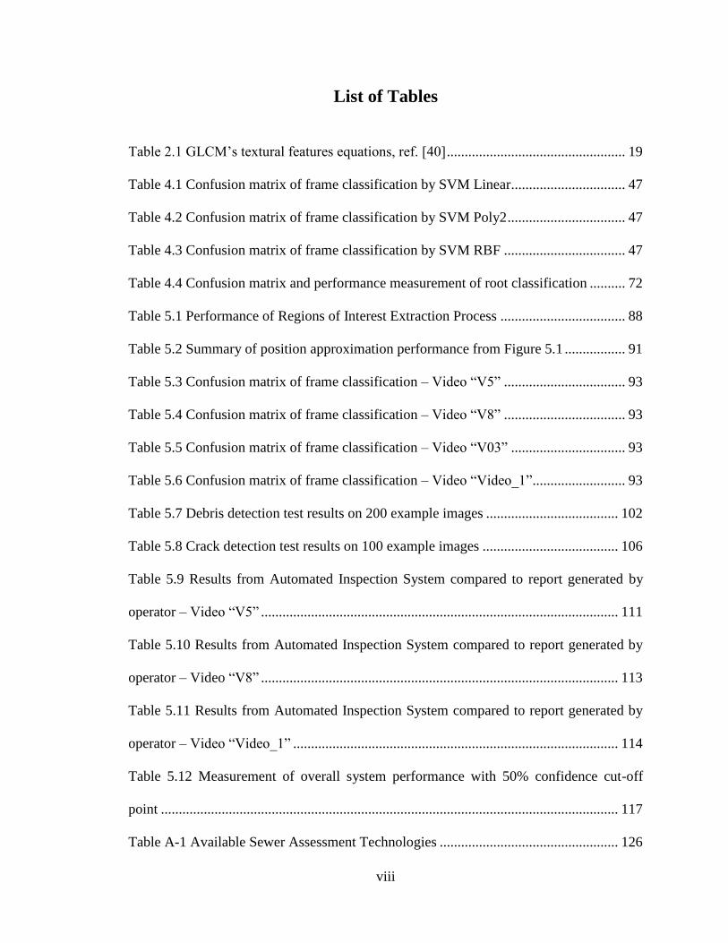
List of Tables
Table 2.1 GLCM’s textural features equations, ref. [40] .................................................. 19
Table 4.1 Confusion matrix of frame classification by SVM Linear................................ 47
Table 4.2 Confusion matrix of frame classification by SVM Poly2 ................................. 47
Table 4.3 Confusion matrix of frame classification by SVM RBF .................................. 47
Table 4.4 Confusion matrix and performance measurement of root classification .......... 72
Table 5.1 Performance of Regions of Interest Extraction Process ................................... 88
Table 5.2 Summary of position approximation performance from Figure 5.1 ................. 91
Table 5.3 Confusion matrix of frame classification – Video “V5” .................................. 93
Table 5.4 Confusion matrix of frame classification – Video “V8” .................................. 93
Table 5.5 Confusion matrix of frame classification – Video “V03” ................................ 93
Table 5.6 Confusion matrix of frame classification – Video “Video_1”.......................... 93
Table 5.7 Debris detection test results on 200 example images ..................................... 102
Table 5.8 Crack detection test results on 100 example images ...................................... 106
Table 5.9 Results from Automated Inspection System compared to report generated by
operator – Video “V5” .................................................................................................... 111
Table 5.10 Results from Automated Inspection System compared to report generated by
operator – Video “V8” .................................................................................................... 113
Table 5.11 Results from Automated Inspection System compared to report generated by
operator – Video “Video_1” ........................................................................................... 114
Table 5.12 Measurement of overall system performance with 50% confidence cut-off
point ................................................................................................................................ 117
Table A-1 Available Sewer Assessment Technologies .................................................. 126
ix
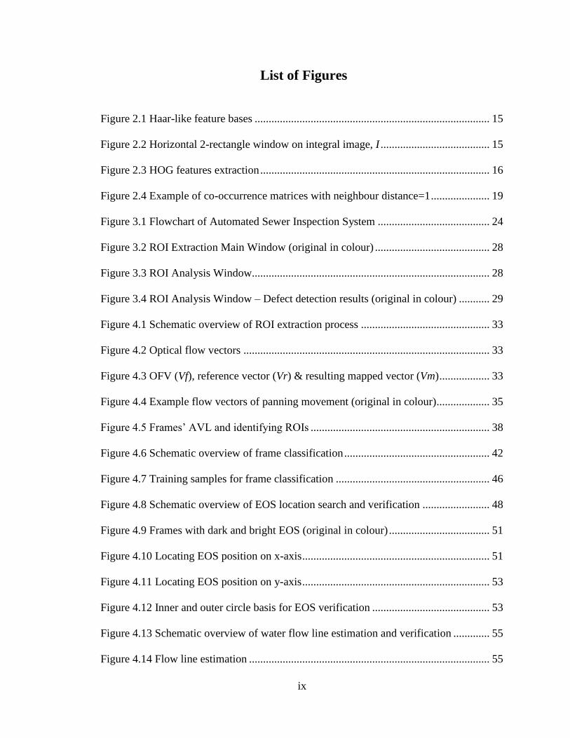
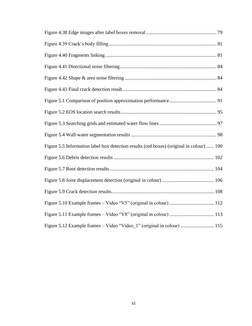
List of Figures
Figure 2.1 Haar-like feature bases .................................................................................... 15
Figure 2.2 Horizontal 2-rectangle window on integral image, I ....................................... 15
Figure 2.3 HOG features extraction .................................................................................. 16
Figure 2.4 Example of co-occurrence matrices with neighbour distance=1 ..................... 19
Figure 3.1 Flowchart of Automated Sewer Inspection System ........................................ 24
Figure 3.2 ROI Extraction Main Window (original in colour) ......................................... 28
Figure 3.3 ROI Analysis Window..................................................................................... 28
Figure 3.4 ROI Analysis Window – Defect detection results (original in colour) ........... 29
Figure 4.1 Schematic overview of ROI extraction process .............................................. 33
Figure 4.2 Optical flow vectors ........................................................................................ 33
Figure 4.3 OFV (Vf), reference vector (Vr) & resulting mapped vector (Vm) .................. 33
Figure 4.4 Example flow vectors of panning movement (original in colour)................... 35
Figure 4.5 Frames’ AVL and identifying ROIs ................................................................ 38
Figure 4.6 Schematic overview of frame classification .................................................... 42
Figure 4.7 Training samples for frame classification ....................................................... 46
Figure 4.8 Schematic overview of EOS location search and verification ........................ 48
Figure 4.9 Frames with dark and bright EOS (original in colour) .................................... 51
Figure 4.10 Locating EOS position on x-axis ................................................................... 51
Figure 4.11 Locating EOS position on y-axis ................................................................... 53
Figure 4.12 Inner and outer circle basis for EOS verification .......................................... 53
Figure 4.13 Schematic overview of water flow line estimation and verification ............. 55
Figure 4.14 Flow line estimation ...................................................................................... 55

x
Figure 4.15 Grey intensity plotting along one horizontal scan line .................................. 55
Figure 4.16 Schematic overview of wall-water segmentation .......................................... 57
Figure 4.17 Wall-water segmentation ............................................................................... 57
Figure 4.18 Extracted wall and water segments (original in colour) ................................ 58
Figure 4.19 Schematic overview of information label boxes detection ............................ 60
Figure 4.20 Information label box detection (original in colour) ..................................... 60
Figure 4.21 Schematic overview of debris detection ........................................................ 63
Figure 4.22 Debris candidate detection............................................................................. 63
Figure 4.23 Finalizing debris candidate detection with label box removal ...................... 64
Figure 4.24 Show examples of detected/rejected debris ................................................... 64
Figure 4.25 Schematic overview of root detection ........................................................... 66
Figure 4.26 Root candidate detection ............................................................................... 68
Figure 4.27 Root detection result ...................................................................................... 68
Figure 4.28 Training samples for root recognition ........................................................... 71
Figure 4.29 ROC Curve of root classification on 100 test images ................................... 72
Figure 4.30 Schematic overview of joint displacement detection .................................... 74
Figure 4.31 Joint displacement frames ............................................................................. 74
Figure 4.32 Joint displacement detection basis ................................................................. 74
Figure 4.33 Plot of subtraction score vs. detecting radius ................................................ 75
Figure 4.34 Schematic overview of crack detection ......................................................... 78
Figure 4.35 Comparison of edge detection methods ........................................................ 78
Figure 4.36 Detected edges using Sobel ........................................................................... 79
Figure 4.37 Label boxes detection on horizontal-edge image (original in colour) ........... 79
xi
Figure 4.38 Edge images after label boxes removal ......................................................... 79
Figure 4.39 Crack’s body filling ....................................................................................... 81
Figure 4.40 Fragments linking .......................................................................................... 81
Figure 4.41 Directional noise filtering .............................................................................. 84
Figure 4.42 Shape & area noise filtering .......................................................................... 84
Figure 4.43 Final crack detection result ............................................................................ 84
Figure 5.1 Comparison of position approximation performance ...................................... 91
Figure 5.2 EOS location search results ............................................................................. 95
Figure 5.3 Searching grids and estimated water flow lines .............................................. 97
Figure 5.4 Wall-water segmentation results ..................................................................... 98
Figure 5.5 Information label box detection results (red boxes) (original in colour) ....... 100
Figure 5.6 Debris detection results ................................................................................. 102
Figure 5.7 Root detection results .................................................................................... 104
Figure 5.8 Joint displacement detection (original in colour) .......................................... 106
Figure 5.9 Crack detection results................................................................................... 108
Figure 5.10 Example frames – Video “V5” (original in colour) .................................... 112
Figure 5.11 Example frames – Video “V8” (original in colour) .................................... 113
Figure 5.12 Example frames – Video “Video_1” (original in colour) ........................... 115

xii
List of Appendices
Appendix A Summary of Available Sewer Assessment Technologies .......................... 126
Appendix B Example of Automated Sewer Inspection’s XML Report.......................... 128
Appendix C Example of Operator’s Excel Report.......................................................... 135
xiii
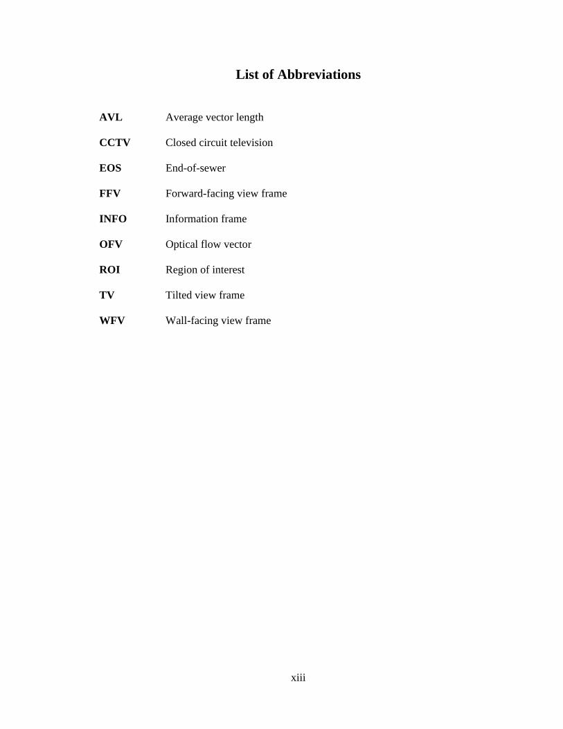
List of Abbreviations
AVL Average vector length
CCTV Closed circuit television
EOS End-of-sewer
FFV Forward-facing view frame
INFO Information frame
OFV Optical flow vector
ROI Region of interest
TV Tilted view frame
WFV Wall-facing view frame
1
Chapter 1
INTRODUCTION
1.1 Background and Introduction
North American municipalities have been using Closed Circuit Television (CCTV) as the
primary sewer inspection technique for over 40 years [28]. Sewer condition information
is an important tool for developing asset management and renewal planning strategies.
Several other sewer inspection technologies, such as sonar/ultrasonic techniques, sewer
scanning and evaluation technology (SSET), laser-based scanning, focused electrode leak
location (FELL), and ground penetrating radars (GPR) have rapidly advanced over the
last two decades. However, these technologies still have limited use in the industry, and
CCTV technology remains the most widely used sewer inspection technology.
CCTV videos are captured by a robot-mounted pan-tilt-and-zoom camera traveling
through sewer mains between manholes. CCTV sewer inspections are highly dependent
on the operator’s interpretation and assessment, and hence, could be somewhat
subjective. Also, operators may be subject to fatigue due to lengthy inspection sessions,
which could lead to erroneous assessment of the sewer condition.
2
Sewer historical condition information is very important in order to develop deterioration
models for the purpose of future condition prediction, asset management, and renewal
planning strategies. Developing such models would be far more cost-effective if there
were a technology that enabled the condition assessment to be automatically done and
with a consistent rating scheme.
To address these issues, this research focuses on the development of a solution that assists
CCTV inspection of sewer condition by using image and video processing techniques.
This thesis solely focuses on studying and implementing an effective automatic defect
detection system prototype from sewer CCTV video files.
1.2 Research Objectives
The purpose of this research is to develop and validate algorithms and a software
prototype to support automated analysis and defect detection in sewer CCTV videos. The
prototype will help reduce the time required for sewer inspection and evaluation
processes, as well as allowing inspection data to be better managed.
The following are the main requirements of the system in order to meet our objectives:
1. Implement an off-line sewer inspection system that focuses on inspecting CCTV
videos from archives of historical records. Historical condition data is very
important for rehabilitation planning and future condition prediction.
2. Reduce time and cost and improve consistency and accuracy of inspection and
condition assessment data.
3
3. Minimize user inputs and try to automate the process as much as possible.
4. Allow revisiting for reviewing results by users if needed
5. Analyze camera motion to locate traveled distance of camera, which is required
for location reference of detected defects.
6. Reduce number of frames with possible potential defects to shorten processing
time.
7. Effectively detect sewer defects, and identify defects type and position.
8. Estimate a priority ranking to get first attention for repair upon requirement.
1.3 Scope and Limitations
The prototype software was built and tested on a set of CCTV video files provided by the
City of Regina, which may restrict the software scope and its detection ability to some
specific characteristic of the test case sewers and defects. The system was implemented
and tested using CCTV videos of sewer material type Concrete and Vitrified Clay Tile
(VCT) of a circular shape with diameter sizes ranging from 250 mm to 900 mm. The
video format is MPEG-1 with a frame width of 320 to 352 pixels and height of 240
pixels. Only four types of defects are currently considered: debris, tree root intrusion,
joint displacement, and cracks. Other defects such as sewer collapse, breakage,
deformation, and wall encrustation, as well as different materials or structures of sewers,
such as brick, can be added in future work when more defective sewer examples become
available.
4
1.4 Overview of Technical Approach
Several new algorithms are proposed to support automated identification of regions of
interest (ROI) in the CCTV videos, classification of frames based on camera orientation,
segmentation using grey-level intensity analysis, and automated detection of several
sewer defects. There are three main processes implemented to achieve the project’s
objectives, which include: Regions of Interest Extraction, Sewer Image Segmentation,
and Defect Detection.
Starting from a raw CCTV video, the system’s operation begins by performing camera
motion analysis to identify and locate the ROI inside the sewer. These ROI represent
`suspicious` video segments where sewer defects (or other interesting features) are more
likely to be present. Frames within the identified ROI are further processed and analyzed
to extract useful information and identify existing defects, if any. The methodology to
automatically extract the ROI in a CCTV video is based on the observation that the
operator’s behaviour and actions during the inspection session are often reflected in
changes to the camera motion sequences, which could be used to indirectly indicate the
presence of the ROI. An optical flow algorithm [9] was used and adapted to calculate
distance travelling inside tubing characteristic of sewers, as well as to identify suspicious
video sections, called Regions of Interest (ROIs), instead of inspecting the whole length
so as to lessen the processing work. A number of algorithms were developed to segment
individual frames and to automatically detect and classify structural and operational
defects. Sewer frame segmentation and defect detection algorithms were developed using
various image processing, edge detection, the Hough Transforms algorithm, and Grey-
5
Level Co-Occurrence Matrix (GLCM). More information and software implementation
details are described in Chapter 3 and Chapter 4.
The proposed system is composed of three main components. The main component was
implemented in C++ using Intel’s Open Computer Vision library (OpenCV). This
component provides users with a graphical interface that was created using the Microsoft
Foundation Class (MFC) library. Through the graphical user interface, users can
transparently access all functions provided by other software components. The second
component was developed using MATLAB software and its Image Processing toolbox.
This component consisted primarily of a set of MATLAB scripts that implemented the
segmentation and defect detection algorithms. The third component included the SVMlight
software. The system was built and tested using a set of CCTV videos obtained from the
City of Regina, Canada.
1.5 Organization
This thesis is divided into 6 chapters. Chapter 2 includes the review of previous work of
sewer defect detection and related topic. An overview of the system design is presented in
Chapter 3, followed by a description of the proposed algorithms in Chapter 4. Chapter 5
discusses the testing results and the software evaluation process. Finally, Chapter 6
describes the performance results and suggestions for possible future work.

6
Chapter 2
RELATED WORK AND TOOLS
2.1 Previous Work
This section provides a review of some previous research projects that focused on
implementing automated condition assessment of sewer pipelines using image processing
and various other techniques.
2.1.1 Automated Sewer Defect Detection and Condition Assessment
Sinha et al. [50] have proposed automated condition assessment on unfolded images of
sewer pipe surfaces obtained from sewer scanner and evaluation technology (SSET). A
cracks detection algorithm was developed based on morphological segmentation and a
Neuro-Fuzzy Network classifier [47],[50]. Other crack detection methods have also been
proposed, such as a statistical filters-based crack detector [36],[46] and cross-curvature
evaluation using a Laplacian operator [42],[43].
Moselhi and Shehab [33],[53] have proposed automated detection and classification of
defects in sewer pipes by employing image processing for segmentation, image analysis
for feature extraction, and neural networks for defect classification.
7
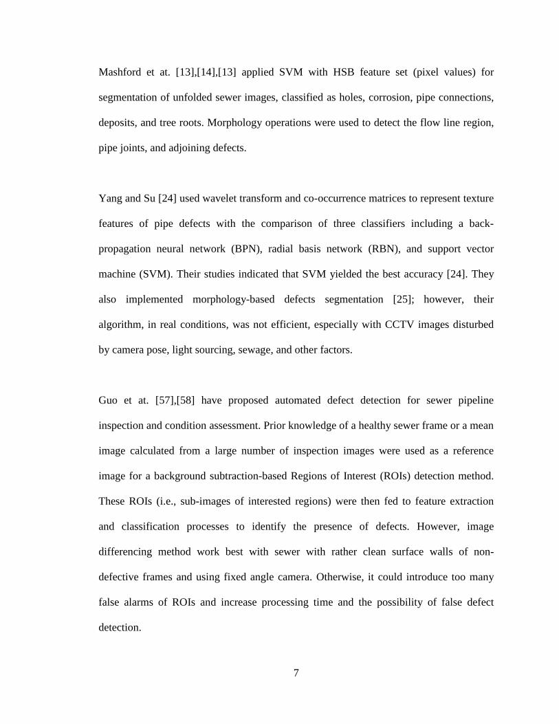
Mashford et at. [13],[14],[13] applied SVM with HSB feature set (pixel values) for
segmentation of unfolded sewer images, classified as holes, corrosion, pipe connections,
deposits, and tree roots. Morphology operations were used to detect the flow line region,
pipe joints, and adjoining defects.
Yang and Su [24] used wavelet transform and co-occurrence matrices to represent texture
features of pipe defects with the comparison of three classifiers including a back-
propagation neural network (BPN), radial basis network (RBN), and support vector
machine (SVM). Their studies indicated that SVM yielded the best accuracy [24]. They
also implemented morphology-based defects segmentation [25]; however, their
algorithm, in real conditions, was not efficient, especially with CCTV images disturbed
by camera pose, light sourcing, sewage, and other factors.
Guo et at. [57],[58] have proposed automated defect detection for sewer pipeline
inspection and condition assessment. Prior knowledge of a healthy sewer frame or a mean
image calculated from a large number of inspection images were used as a reference
image for a background subtraction-based Regions of Interest (ROIs) detection method.
These ROIs (i.e., sub-images of interested regions) were then fed to feature extraction
and classification processes to identify the presence of defects. However, image
differencing method work best with sewer with rather clean surface walls of non-
defective frames and using fixed angle camera. Otherwise, it could introduce too many
false alarms of ROIs and increase processing time and the possibility of false defect
detection.
8
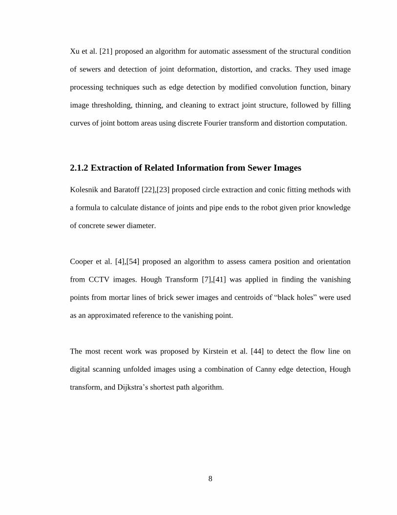
Xu et al. [21] proposed an algorithm for automatic assessment of the structural condition
of sewers and detection of joint deformation, distortion, and cracks. They used image
processing techniques such as edge detection by modified convolution function, binary
image thresholding, thinning, and cleaning to extract joint structure, followed by filling
curves of joint bottom areas using discrete Fourier transform and distortion computation.
2.1.2 Extraction of Related Information from Sewer Images
Kolesnik and Baratoff [22],[23] proposed circle extraction and conic fitting methods with
a formula to calculate distance of joints and pipe ends to the robot given prior knowledge
of concrete sewer diameter.
Cooper et al. [4],[54] proposed an algorithm to assess camera position and orientation
from CCTV images. Hough Transform [7],[41] was applied in finding the vanishing
points from mortar lines of brick sewer images and centroids of “black holes” were used
as an approximated reference to the vanishing point.
The most recent work was proposed by Kirstein et al. [44] to detect the flow line on
digital scanning unfolded images using a combination of Canny edge detection, Hough
transform, and Dijkstra’s shortest path algorithm.
9
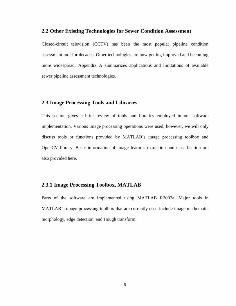
2.2 Other Existing Technologies for Sewer Condition Assessment
Closed-circuit television (CCTV) has been the most popular pipeline condition
assessment tool for decades. Other technologies are now getting improved and becoming
more widespread. Appendix A summarizes applications and limitations of available
sewer pipeline assessment technologies.
2.3 Image Processing Tools and Libraries
This section gives a brief review of tools and libraries employed in our software
implementation. Various image processing operations were used; however, we will only
discuss tools or functions provided by MATLAB’s image processing toolbox and
OpenCV library. Basic information of image features extraction and classification are
also provided here.
2.3.1 Image Processing Toolbox, MATLAB
Parts of the software are implemented using MATLAB R2007a. Major tools in
MATLAB’s image processing toolbox that are currently used include image mathematic
morphology, edge detection, and Hough transform.
10
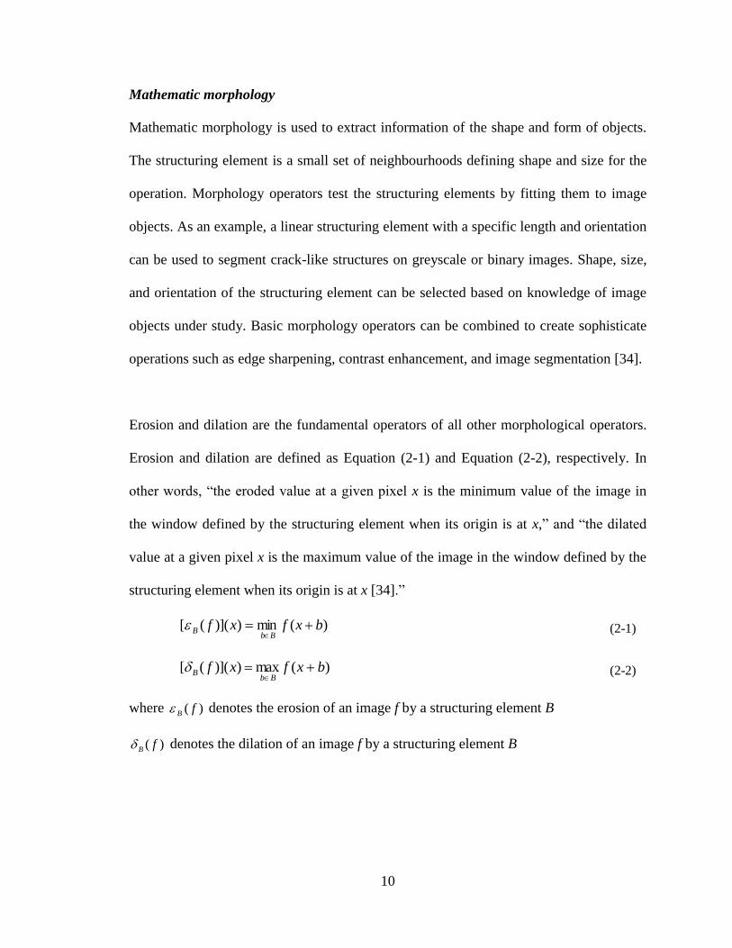
Mathematic morphology
Mathematic morphology is used to extract information of the shape and form of objects.
The structuring element is a small set of neighbourhoods defining shape and size for the
operation. Morphology operators test the structuring elements by fitting them to image
objects. As an example, a linear structuring element with a specific length and orientation
can be used to segment crack-like structures on greyscale or binary images. Shape, size,
and orientation of the structuring element can be selected based on knowledge of image
objects under study. Basic morphology operators can be combined to create sophisticate
operations such as edge sharpening, contrast enhancement, and image segmentation [34].
Erosion and dilation are the fundamental operators of all other morphological operators.
Erosion and dilation are defined as Equation (2-1) and Equation (2-2), respectively. In
other words, “the eroded value at a given pixel x is the minimum value of the image in
the window defined by the structuring element when its origin is at x,” and “the dilated
value at a given pixel x is the maximum value of the image in the window defined by the
structuring element when its origin is at x [34].”
)(min))](([ bxfxfBb
B
(2-1)
)(max))](([ bxfxfBb
B
(2-2)
where )( fB denotes the erosion of an image f by a structuring element B
)( fB denotes the dilation of an image f by a structuring element B
11
Edge detection
The image processing toolbox in MATLAB provides several edge detection methods
including Sobel, Prewitt, Roberts, Laplacian of Gaussian (LoG), zero-cross, and Canny.
An edge is typically the change of image intensity. There are two main approaches of
edge detection, which are the first-order derivatives by the gradient and the second-order
derivatives by the Laplacian method [39]. Sobel, Prewitt, and Roberts edge detection are
based on gradient methods. An edge can be detected by applying a threshold to gradient
magnitude, and direction can also be determined from gradient orientation. However,
gradient-based methods can return weaker responses for diagonal edges than the
horizontal and vertical edges.
The Canny edge detector was proposed by J. Canny [11]. The Canny operator uses a
Gaussian filter to reduce noise. Then, two thresholds are applied to the gradient
magnitude of the Gaussian-smoothed image to detect a wide range of edges (strong and
weak edges) based on hysteresis method.
LoG for edge detection was presented by Marr and Hildreth [5]. LoG edge detection is
based on Laplacian method (i.e., by searching for zero crossings in the second derivative
of images). In general, Laplacian method is not suitable for the edge detection
applications due to its sensitivity to noise and inability to get edge directional information
[39].
12
In our crack detection algorithm, Sobel, Canny, and LoG edge detection methods were
tested and compared. Edge images returned by Sobel method had suitable characteristics
for our application. Our recent work uses Sobel edge detection with automatic assignment
of sensitivity threshold (MATLAB’s default) based on Abdou and Pratt’s conclusion that
“the edge detection threshold can be scaled linearly with signal-to-noise ratio” [59].
Hough transform algorithm
The Hough transform functions provided in MATLAB’s image processing toolbox are
based on Duda and Hart’s algorithm [41]. Hough transform was first introduced by
Hough [37] in 1962 and improved by Duda and Hart [41] for line and curve detection in
digital images.
Hough transformed lines in picture planes to 2D parameters represented by slope and
intercept, which are m and b parameters of a straight line y = mx + b. To solve the
unbounded problem of slope and intercept value, Duda and Hart suggested alternative
parameterization by introducing θ - ρ plane. Angle (θ) and distance (ρ) from the origin
can represent a line by ρ = x cos θ + y sin θ. Peaks or points at the most frequent
intersection in the parameter space can be detected to obtain the fitting lines. This
transformation concept can be extended to detect other shapes or curves by defining their
parametric representation and transforming points in picture space to parameter space
[41]. Generally, edge detection is applied for pre-processing before using Hough
transform to detect line or curve candidates from image pixels.
13
2.3.2 OpenCV Library
OpenCV1 is a famous open source library for realtime computer vision. It is written in C
and C++ with interfaces for Python, Ruby, MATLAB, and other languages [9]. OpenCV
runs under Linux, Windows, and Mac OS X with more than 500 functions in vision areas.
Optical flow
Optical flow is a tool that can be used to assess motion between frame sequences by
tracking points (or blocks) of interesting features from one frame to the next frame.
Points of interest for tracking can be extracted from images using functions based on the
Shi and Tomasi algorithm [16] provided by OpenCV Library. The tracking method we
used is called Pyramidal Lucas-Kanade optical flow, which is the most popular technique
originating from the Lucas-Kanade (LK) algorithm [2] among other available techniques
such as block matching [51],[60] and the Horn-Schunck method [3]. The LK algorithm
works by tracking points of interest in the surrounding small windows. A problem,
however, arises when the point of interest moves outside the local window with a fast
motion. Image pyramid was then developed to estimate optical flow from coarse to fine
detail, allowing faster and longer motion tracking [9].
2.3.3 Image features extraction
Image features are the representatives of image characteristic, which are normally
required for image segmentation and image classification applications. One example is to
use the pixel values of the image directly; however, this approach is not efficient due to
1 OpenCV library is available at http://SourceForge.net/projects/opencvlibrary

14
the very large feature space, and it causes complexity, is time consuming, and lowers
process performance. Many works have suggested effective features extraction methods
to obtain image attributes such as intensity or colour, shape, and texture by some specific
manipulations. Haar wavelet, HOG, and GLCM are being used in our current work.
Haar Wavelet
Mallat [45] extended the wavelet model of 1D signals to work on 2D image processing
applications and defined orthogonal multi-resolution wavelet representation. Viola and
Jones [35] further introduced integral images for more rapid feature evaluation. “Integral
image at location x, y contains the sum of the pixels above and to the left of x, y, inclusive
[35].” An integral image is computed only once over the original image, and then, any
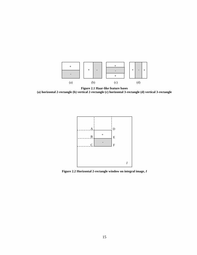
rectangular sum can be easily obtained. Refering to Figure 2.2, the sum of the pixels in
the white rectangle equals (E – D – B+ A) and the sum of the pixels in the grey rectangle
is (F – E – C + B).
We selected four Haar bases for our implementation including horizontal two-rectangle,
vertical two-rectangle, horizontal three-rectangle, and vertical three-rectangle as shown in
Figure 2.1. Features are calculated by subtracting the sum of pixels in white boxes by the
sum of pixels in grey boxes. Two-rectangle features can be computed from the integral
image involving 6 reference points, and three-rectangle computation involves 8 points.
For example, the horizontal two-rectangle feature value in Figure 2.2 can be computed by
(E – D – B+ A) - (F – E – C + B), which is equivalent to (A – 2B + C – D + 2E – F).
15
Figure 2.1 Haar-like feature bases
(a) horizontal 2-rectangle (b) vertical 2-rectangle (c) horizontal 3-rectangle (d) vertical 3-rectangle
Figure 2.2 Horizontal 2-rectangle window on integral image, I
+
-
(a)
+ -
(b)
+
-
+
(c)
+ + -
(d)
+
-
I
A
B
C
D
E
F
16
(a)
(b)
(c)
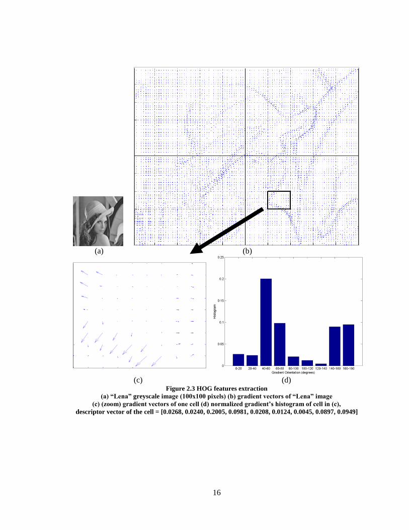
(d) Figure 2.3 HOG features extraction
(a) “Lena” greyscale image (100x100 pixels) (b) gradient vectors of “Lena” image
(c) (zoom) gradient vectors of one cell (d) normalized gradient’s histogram of cell in (c),
descriptor vector of the cell = [0.0268, 0.0240, 0.2005, 0.0981, 0.0208, 0.0124, 0.0045, 0.0897, 0.0949]
17
Histograms of Oriented Gradients (HOG)
Orientation-based histogram features were first introduced by Mikolajczyk et al. [20] for
body parts detection. HOG was extended by Dalal and Triggs [30] to detect humans in a
single detection window with experiments involving various computation methods and
parameters.
For best performance, we followed the HOG implementation and parameters suggested
by Dalal and Triggs [30], including using a simple 1-D gradient filter mask [-1 0 1] with
no smoothing, 9 orientation bins with equal space over 0-180 degrees to collect the
magnitude of unsigned gradients, and L2-norm for local (block) contrast normalization.
To reduce complexity, we computed HOG on greyscale images instead of 3 channel
colour images. Cell size is 10x10 pixels with square blocks of 5x5 cells non-overlapping.
To extract HOG features, an image is first divided into small cells. Gradients are then
computed for every pixel in a cell (i.e., by convolution with a gradient filter). Gradient
magnitude is accumulated into a histogram bin in accordance with its orientation.
Magnitude and orientation can be computed with Equation (2-3) and Equation (2-4).
Histograms are normalized locally (over a larger block); refer to Equation (2-5) for L2-
norm normalization. Figure 2.3(d) shows the normalized histogram of one cell. The final
descriptor vector is the collection of all normalized histograms. One detection image will
have a total of (4 blocks x 25 cells per block x 9 bins) = 900 elements of the HOG
descriptor.
18
),(),(),( 22 yxGyxGyxG vh (2-3)
),(),(tan),( 1 yxGyxGyx hv
(2-4)
where: Gh(x,y), Gv(x,y)= gradient in horizontal and vertical direction, at pixel (x,y)
22
2 vvvnorm
(2-5)
where: ||v||2 = 2-norm of descriptor vector (v), and ε = small constant
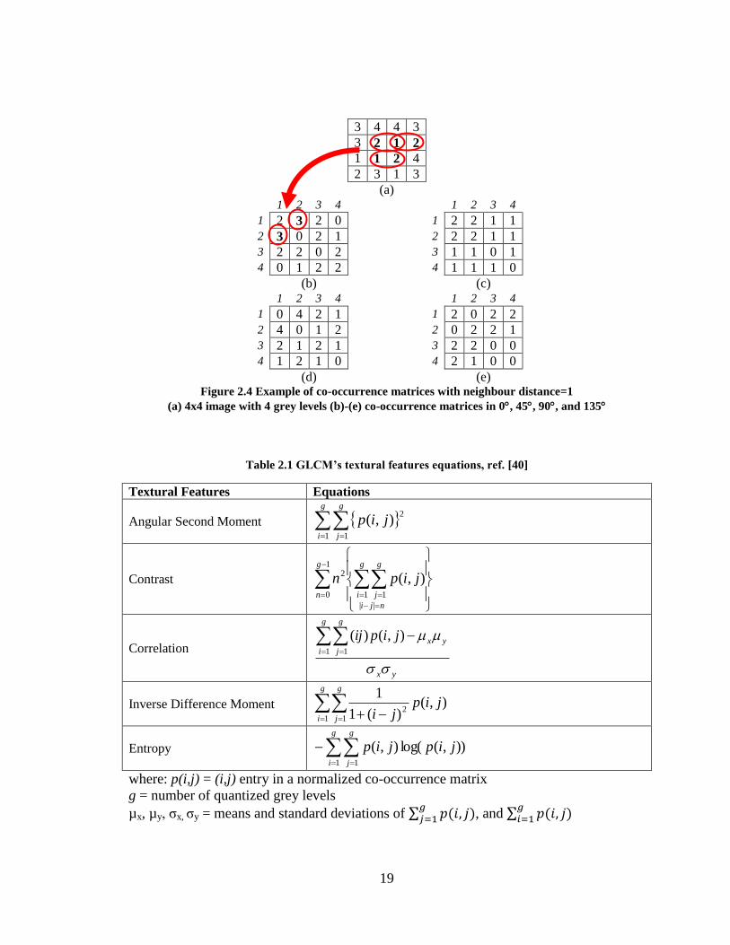
Grey-Level Co-Occurrence Matrix (GLCM)
The grey-level co-occurrence matrix (GLCM) [40] is a well-known texture analysis
method that extracts statistical texture information from a spatial co-occurrence matrix.
Examples of textural GLCM features include angular second moment (or energy),
contrast, correlation, variance, and entropy.
The very first step of GLCM computation is to create co-occurrence matrices in various
orientations. A greyscale image that consists of 256 grey levels is usually quantized to
lower levels such as 8, 16, 32, or 64 to reduce computation cost. Let g be the total number
of quantized grey levels. The co-occurrence matrix will have a size of g x g, with
elements at (i, j) equal to the number of occurrences in which grey tones i and j are
neighbours. See Figure 2.4 for an example of co-occurrence matrices using 1 pixel
neighbour distance in 0, 45, 90, and 135 directions. The matrices are then normalized
by dividing by total number of neighbouring pairs. Image size h x w will have a total of
2h(w-1) nearest horizontal neighbour pairs, 2w(h-1) nearest vertical pairs, and 2(h-1)(w-
1) nearest diagonal pairs. Statistical features can be calculated from the co-occurrence
matrices. Table 2.1 shows equations of some of GLCM’s textural features.
19
3 4 4 3
3 2 1 2
1 1 2 4
2 3 1 3
(a)
1 2 3 4 1 2 3 4
1 2 3 2 0 1 2 2 1 1
2 3 0 2 1 2 2 2 1 1
3 2 2 0 2 3 1 1 0 1
4 0 1 2 2 4 1 1 1 0
(b) (c)
1 2 3 4 1 2 3 4
1 0 4 2 1 1 2 0 2 2
2 4 0 1 2 2 0 2 2 1
3 2 1 2 1 3 2 2 0 0
4 1 2 1 0 4 2 1 0 0
(d) (e) Figure 2.4 Example of co-occurrence matrices with neighbour distance=1
(a) 4x4 image with 4 grey levels (b)-(e) co-occurrence matrices in 0, 45, 90, and 135
Table 2.1 GLCM’s textural features equations, ref. [40]
Textural Features Equations
Angular Second Moment
g
i
g
j
jip1 1
2),(
Contrast
1
0
||
1 1
2 ),(g
n
nji
g
i
g
j
jipn
Correlation
yx
g
i
g
j
yxjipij
1 1
),()(
Inverse Difference Moment
g
i
g
j
jipji1 1
2),(
)(1
1
Entropy
g
i
g
j
jipjip1 1
)),(log(),(
where: p(i,j) = (i,j) entry in a normalized co-occurrence matrix
g = number of quantized grey levels
µx, µy, σx, σy = means and standard deviations of ∑ , and ∑
20
2.3.4 Classification tool
The classification process usually involves preprocessing and collecting features that
represent training/testing data as already discussed in the previous sub-section.
Classification or pattern recognition problems, in general, are to predict which class a
new, unseen object belongs to, after a proper learning process.
Support Vector Machine (SVM) and Neural Networks are currently the most popular
classification techniques. SVM is employed in our current work; however, Neural
Networks can also be considered as an alternative classifier.
Support Vector Machine (SVM)
Support Vector Machine (SVM) for pattern recognition was invented by Vapnik [56].
The SVM classifier works by mapping original data vectors to high-dimensional space,
and then, finding the hyperplane that separates classes of data, with largest margin
assigned to the nearest training data points. In the case that no hyperplane is achievable, a
soft margin hyperplane that separates classes as much as possible is selected with a trade
off between margin size and error penalties.
SVMlight 2
implemented by Joachims [52] is a collection of tools, based on Vapnik’s
algorithm, to solve linear/non-linear classification, regression, and ranking problems.
SVMlight
supports both supervised and unsupervised learning. It handles large-scale
learning with a fast optimization algorithm. Available kernel functions include linear,
2 SVM
light is available at http://svmlight.joachims.org/

21
polynomial, radial basis function (RBF), sigmoid tanh, as well as user defined kernels.
SVMlight
also supports multivariate classification, which is implemented in an
optimization fashion (called Structural SVMs) based on Crammer and Singer’s multiclass
algorithm [17].

22
Chapter 3
SYSTEM DESIGN AND IMPLEMENTATION
3.1 System Design Overview
The proposed system aims to support the sewer inspection process by automating the
CCTV video analysis and defect detection. The inspection system is divided into three
main processes, including: Regions of Interest Extraction, Sewer Segmentation, and
Defect Detection.
Regions of Interest Extraction is the first process to recognise suspicious areas, confining
the number of fames for detection process. The process collects groups of suspicious
frames, called Regions of Interest (ROIs). Each ROI contains a set of consecutive frames
of recognised stopping periods, which includes the following camera actions: pausing,
slowing, and interrupted short moving/backing, as well as possible zooming and tilting.
Preliminary severity ranking is also calculated from the number of frames inside a ROI.
Preliminary ranking provides a rough idea of which location of sewer should get more
attention.
During ROI extraction, location parameters are also computed based on both distance and
direction of camera movement (i.e., adding when moving forward or subtracting when
moving backward) for more accurate location estimation. Then, all frames that are of
interest will be classified into 4 categories, including Forward-Facing View (FFV)
23
frames, Tilted View (TV) frames, Wall-Facing View (WFV) frames, and Information
(INFO) frames.
Sewer Segmentation will continue only with FFV frames in ROIs only, and frames in
other categories will be skipped. The segmentation process includes locating the end-of-
sewer (EOS), approximating flow line, and separating wall and water segments. This
segment information is required in defect detection processes, such as debris detection,
and in joint detection. Frames other than FFV type are not applicable and unnecessary for
image segmentation because neither EOS nor water fully appears in WFV and INFO
frames. TV frames, which may consist of all EOS, wall, and water, but in different
(unknown) orientation, are usually very few and can be ignored.
The defect detection integrates techniques of image processing and soft computing,
adapting these to our case study problems. Defects such as root intrusion, cracks, joint
displacements, and debris will be processed according to applicable frame type
categories; more detail will follow in the next chapter.
Figure 3.1 shows a flowchart of the processes as previously described. The following
section explains application implementation, the graphic user interface, reports, and
outputs.

24
Get First/Next Frame
Get Frame Class Type
[Other]
[FFV Frame]
[WFV Frame]
Get First/Next ROI Group
Wall-Water Segmentation
EOS Location Search
Water Flow Line Estimation
SEGMENTATION
[Fail]
[Success]
[Fail]
[Success]
Load CCTV Video Files
ROI Extraction
Location Approximation
ROI Ranking
Frames Classification
Save Extracted ROI Frames & Info
ROI EXTRACTION
De
fects
Co
nfid
en
tia
l S
co
re C
alc
ula
tio
n
Sa
ve
De
fects
-Ma
rke
d Im
ag
e &
Ke
ep
Tra
ck o
f C
urr
en
t F
ram
e's
De
tectin
g R
esu
lts
Debris Detection
Crack Detection
Root Detection
Joint Detection
DEFECTS DETECTION
[Fin
ish]
[More
fra
me(
s)]
Create Inspection Report
[More ROI]
[Finish]
Figure 3.1 Flowchart of Automated Sewer Inspection System
25
3.2 System Implementation
The ROI extraction process and frame classification were built as a static library in C++.
Segmentation and defect detection including debris, root, joint displacement, and cracks
were developed in MATLAB R2007a with the image processing toolbox. MATLAB is
preferred for defect detection implementation in terms of math manipulation, debugging
and testing, comparable robust image tools, and developer’s knowledge and experience.
However all MATLAB codes shall be, in future, re-written or converted to C++ for speed
improvement. GUI was created with MFC Application using Microsoft visual studio
2005. Defect detection functions in MATLAB get executed from GUI and run in the
background using the MATLAB Engine library.
3.2.1 Graphic User Interface
A simple Windows-based Graphic User Interface (GUI) was built for system evaluation
purposes and can also be used as a regular application (i.e., on a single workstation). The
application starts with the main GUI window for video file selection, video preview, and
ROI extraction. The second window is populated when ROI analysis (or defect detection)
continues. Detection results can be reviewed by both text information (i.e. defects type
and confidence) and visual information (i.e., defects-marked images).
26
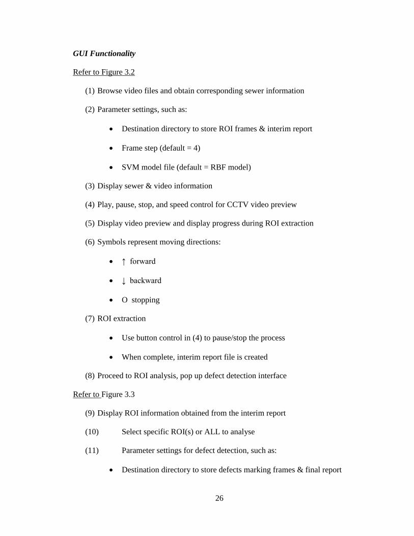
GUI Functionality
Refer to Figure 3.2
(1) Browse video files and obtain corresponding sewer information
(2) Parameter settings, such as:
Destination directory to store ROI frames & interim report
Frame step (default = 4)
SVM model file (default = RBF model)
(3) Display sewer & video information
(4) Play, pause, stop, and speed control for CCTV video preview
(5) Display video preview and display progress during ROI extraction
(6) Symbols represent moving directions:
↑ forward
↓ backward
O stopping
(7) ROI extraction
Use button control in (4) to pause/stop the process
When complete, interim report file is created
(8) Proceed to ROI analysis, pop up defect detection interface
Refer to Figure 3.3
(9) Display ROI information obtained from the interim report
(10) Select specific ROI(s) or ALL to analyse
(11) Parameter settings for defect detection, such as:
Destination directory to store defects marking frames & final report

27
EOS type: Dark, Bright, or Default (evaluate by system)
Any defects to be excluded from the detection process
(12) Run defect detection for selected ROI(s)
Execute MATLAB functions
Use button control in (14) for early termination
When complete, final report is created
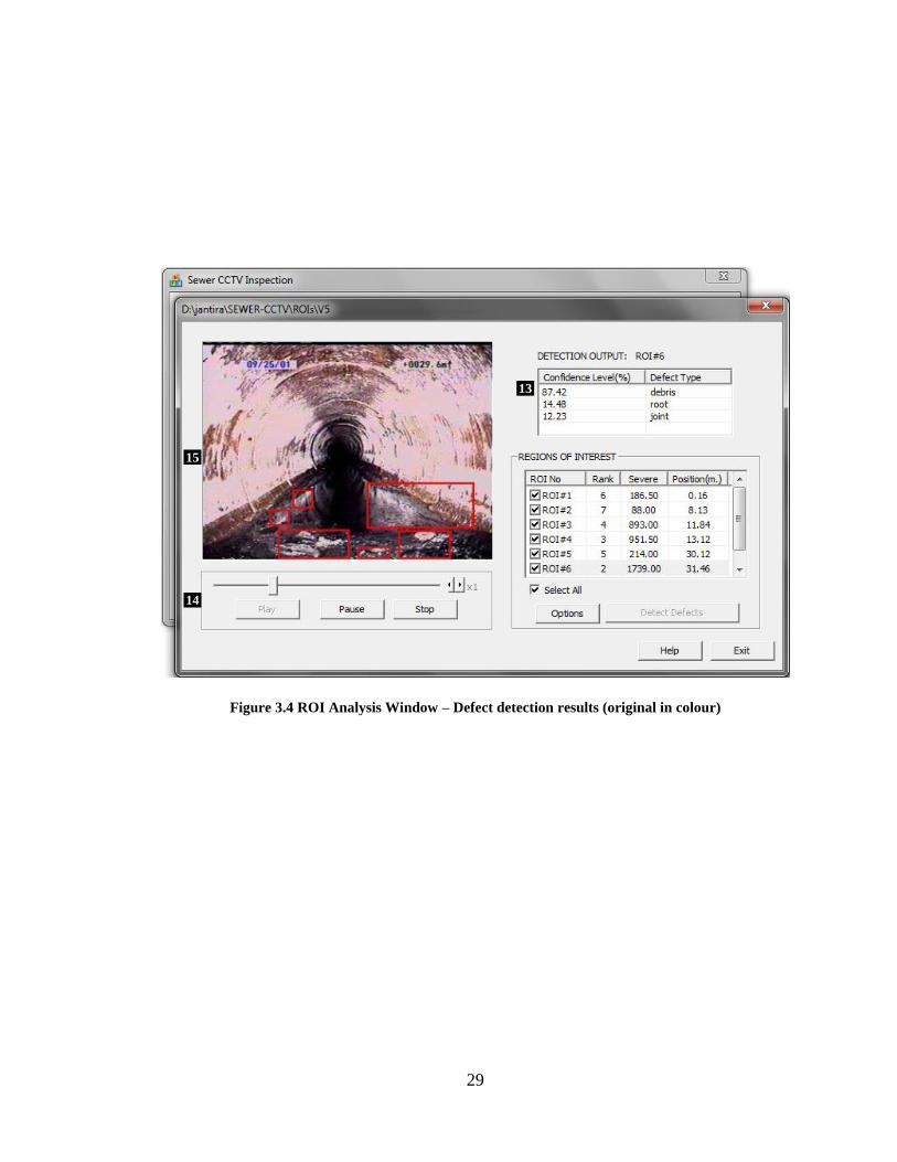
Refer to Figure 3.4
(13) Show detection result, obtained from final report
Double click on (9) to select ROI for information rendering
(14) Play, pause, stop, and speed control to review defect detection result
(15) Display detected defects of ROI frames
Red boxes for roots and debris, red circle for joint displacement, and red
drawing marks around detected cracks
Click/highlight (9) to select which ROI to review

28
Figure 3.2 ROI Extraction Main Window (original in colour)
Figure 3.3 ROI Analysis Window
1 2
3
4
5
6
7
8
11
10
12
9
29
Figure 3.4 ROI Analysis Window – Defect detection results (original in colour)
13
14
15
30
3.2.2 Reports and Outputs
At the completion of the ROI extraction process, an XML interim report is created with
information including video parameters, ROI ID (e.g., “ROI#1”), estimated position (m.),
ranking order, start frame, end frame, and total number of frames in each ROI. All frames
of each ROI group are stored to the directory and sorted into sub-directories according to
frames classes, which are FFV, TV, WFV, and INFO. ROI images will be used in the
defect detection process and can be later deleted to clear up storage space.
A final report is generated once the defect detection process is complete. The final report
is created by appending detection output data, including defect type, confidence level,
start frame, and end frame, to the interim report. In one ROI, defects can be detected in
several groups of consecutive frames instead of the whole length of the ROI. Therefore,
every start and end frame numbers of detected defects are also recorded in the report for
reference purposes. Rectangles, circles, and drawings are marked on sewer frames to
visualize detected defects. Defects-marked frames are saved to the directory for revisiting
review. Examples of interim reports and final reports can be found in Appendix B.
31
Chapter 4
PROPOSED ALGORITHMS
This chapter describes the proposed algorithms and methods of the three main processes,
including Regions of Interest (ROIs) Extraction, Frame Classification and Segmentation,
and Sewer Defect Detection.
4.1 Regions of Interest Extraction
Regions of Interest (ROIs) are short sections of video that are more likely to contain
sewer defects. ROIs help reduce the time of processing the whole length of CCTV video.
Suspicious ROIs can be extracted by using the clue of camera motions. For example,
when any suspicious defects are visible, instead of regular steady-forward movement, the
camera could either stop, slowdown, move backward-forward, and/or other actions such
as panning, tilting, or zooming to interesting areas. This section will discuss the
algorithm, based on optical flow, for detecting camera motions and estimating sewer
location. Figure 4.1 shows the schematic of ROI extraction process.
4.1.1 Optical Flow-Based Techniques
Optical flow assists in tracking the motion of objects or the camera in a video sequence.
The advantages of optical flow over other techniques are the ability to identify movement
direction and to have a higher accuracy of distance estimation.
32
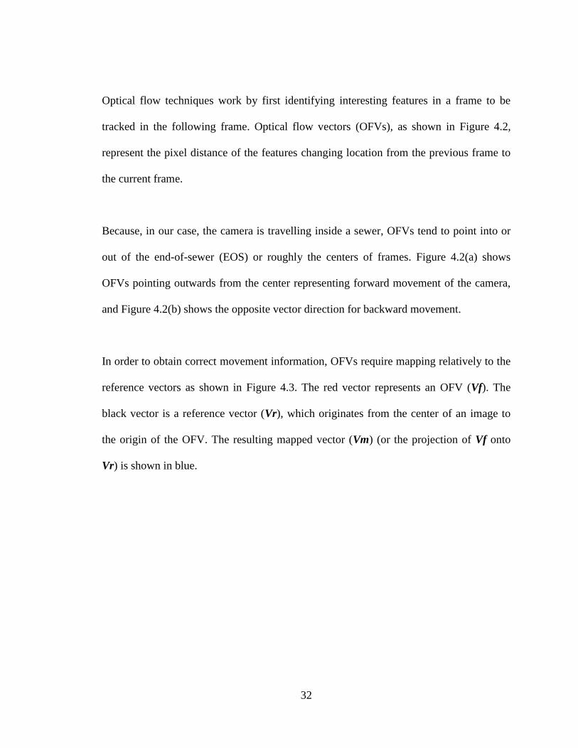
Optical flow techniques work by first identifying interesting features in a frame to be
tracked in the following frame. Optical flow vectors (OFVs), as shown in Figure 4.2,
represent the pixel distance of the features changing location from the previous frame to
the current frame.
Because, in our case, the camera is travelling inside a sewer, OFVs tend to point into or
out of the end-of-sewer (EOS) or roughly the centers of frames. Figure 4.2(a) shows
OFVs pointing outwards from the center representing forward movement of the camera,
and Figure 4.2(b) shows the opposite vector direction for backward movement.
In order to obtain correct movement information, OFVs require mapping relatively to the
reference vectors as shown in Figure 4.3. The red vector represents an OFV (Vf). The
black vector is a reference vector (Vr), which originates from the center of an image to
the origin of the OFV. The resulting mapped vector (Vm) (or the projection of Vf onto
Vr) is shown in blue.
33
Figure 4.1 Schematic overview of ROI extraction process
(a)
(b)
Figure 4.2 Optical flow vectors
(a) forward (b) backward travelling direction (original in colour)
(a)
(b)
Figure 4.3 OFV (Vf), reference vector (Vr) & resulting mapped vector (Vm)
(a) forward (b) backward travelling direction (original in colour)
θ Vm
Vr Vf θ
Vm Vr
Vf
Greyscale Image
Optical flow motion tracking
Map OFV to center
Cal. frame’s AVL & direction, with panning detection
ROIs filtering
Severity ranking
Position estimation
ROIs frames
& position

34
The mapping equation for each individual OFV is
VrVrVf
VfVm
/)(
cos
(4-1)
where: ||Vm|| is the length of the mapped vector, containing length and direction
information (i.e., abs(||Vm||) = vector’s length and sign(||Vm||) = vector’s direction)
Mapped vectors of optical flow yield the following parameters:
Direction Prediction
To determine the movement direction, the number of positive and negative signs of all
valid mapped vectors is counted. If the majority of mapped vectors’ signs in the current
frame is positive, then the camera is moving forward; otherwise, it is moving backward.
Average Vector Length (AVL)
A frame’s average vector length (AVL) can be calculated by averaging all valid mapped
vectors’ lengths (pixels) in the current frame. The resulting AVL will be positive or
negative depending on the direction determined from the previous step. The AVL will be
used to extract ROIs (i.e., identify periods when movement has stopped) and find the
camera’s position in a sewer.
NVmabsdAVLN
i
i /)(1
(4-2)
where: N = number of valid vectors in current frame
d = predicted direction in current frame: forward = +1, backward = -1
35
(a)
(b)
Figure 4.4 Example flow vectors of panning movement (original in colour)
36
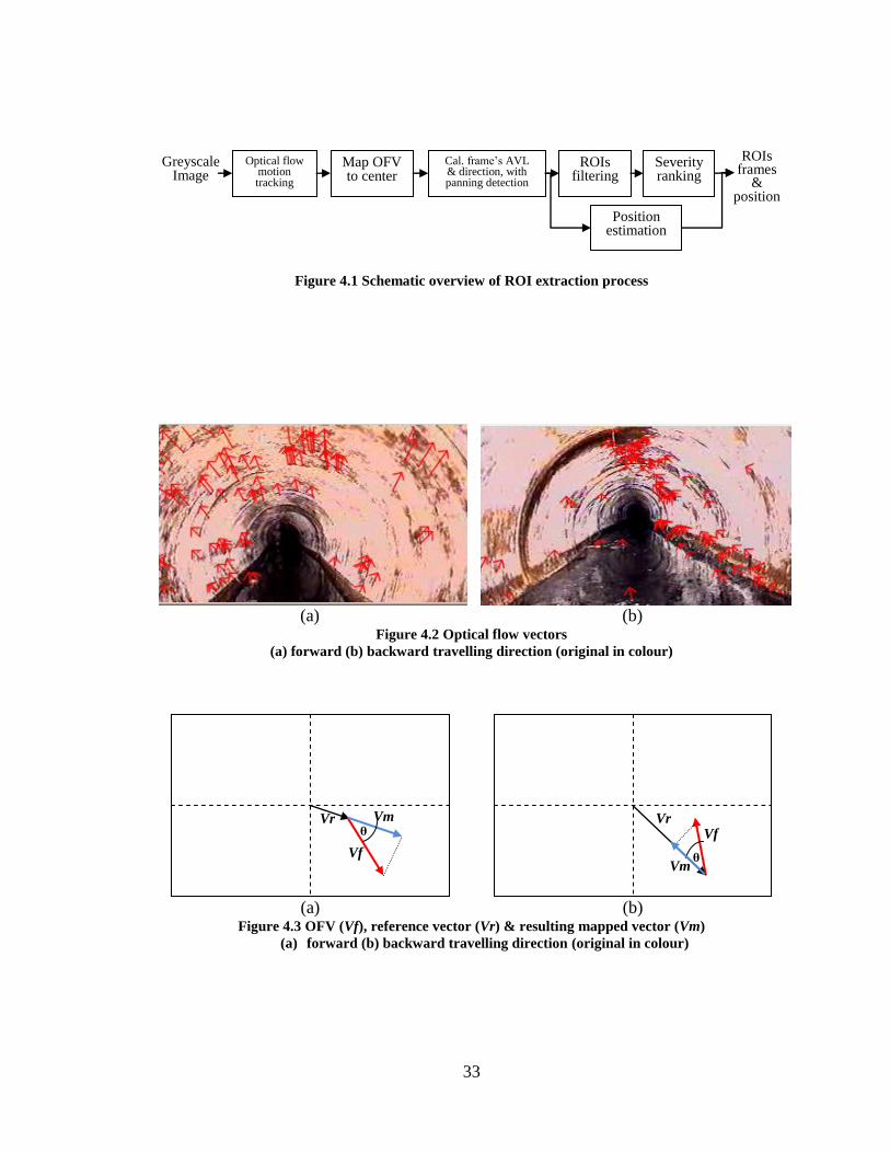
Panning Movement Error Reduction
In some cases, the calculated AVL is not always zero or close to zero when the camera
stops travelling; for example, when the camera is bouncing up or down or panning to the
wall without changing its position. These vectors can cause significant error in the
distance estimation due to the fast movement and, hence, the large vector size, as seen in
Figure 4.4.
Notice that, in the case of movement error, the OFVs all point in the same direction
instead of pointing inward or outward from the frame center. Therefore, the angles of
OFVs can indicate whether it is normal distance movement or error movement.
)/(tan 1
xy VfVf (4-3)
where: ||Vfx|| = OFV’s length in x-axis
||Vfy|| = OFV’s length in y-axis
= angle in degrees, 180180
After the calculation of Equation (4-3) for every OFV, we can conclude that the camera
has normal forward/backward movement if the difference between the minimum and the
maximum angles is greater than 30 degrees. If the movement is identified as panning, the
AVL of that frame will be set to 0 (meaning no travelling distance).
37
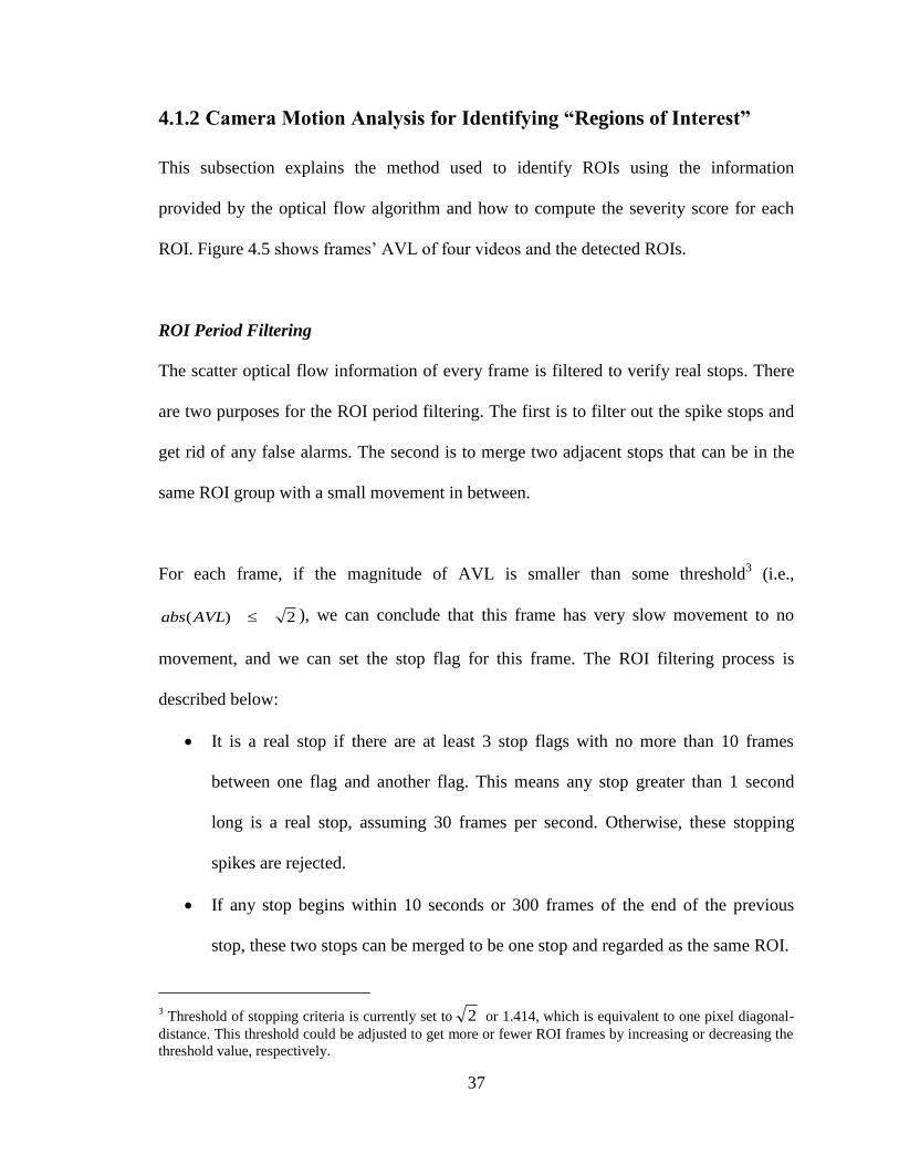
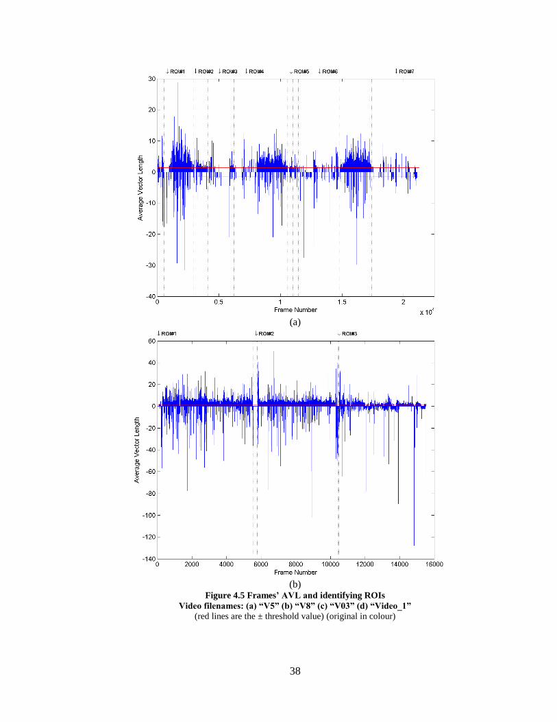
4.1.2 Camera Motion Analysis for Identifying “Regions of Interest”
This subsection explains the method used to identify ROIs using the information
provided by the optical flow algorithm and how to compute the severity score for each
ROI. Figure 4.5 shows frames’ AVL of four videos and the detected ROIs.
ROI Period Filtering
The scatter optical flow information of every frame is filtered to verify real stops. There
are two purposes for the ROI period filtering. The first is to filter out the spike stops and
get rid of any false alarms. The second is to merge two adjacent stops that can be in the
same ROI group with a small movement in between.
For each frame, if the magnitude of AVL is smaller than some threshold3 (i.e.,
2)( AVLabs ), we can conclude that this frame has very slow movement to no
movement, and we can set the stop flag for this frame. The ROI filtering process is
described below:
It is a real stop if there are at least 3 stop flags with no more than 10 frames
between one flag and another flag. This means any stop greater than 1 second
long is a real stop, assuming 30 frames per second. Otherwise, these stopping
spikes are rejected.
If any stop begins within 10 seconds or 300 frames of the end of the previous
stop, these two stops can be merged to be one stop and regarded as the same ROI.
3 Threshold of stopping criteria is currently set to 2 or 1.414, which is equivalent to one pixel diagonal-
distance. This threshold could be adjusted to get more or fewer ROI frames by increasing or decreasing the
threshold value, respectively.
38
(a)
(b)
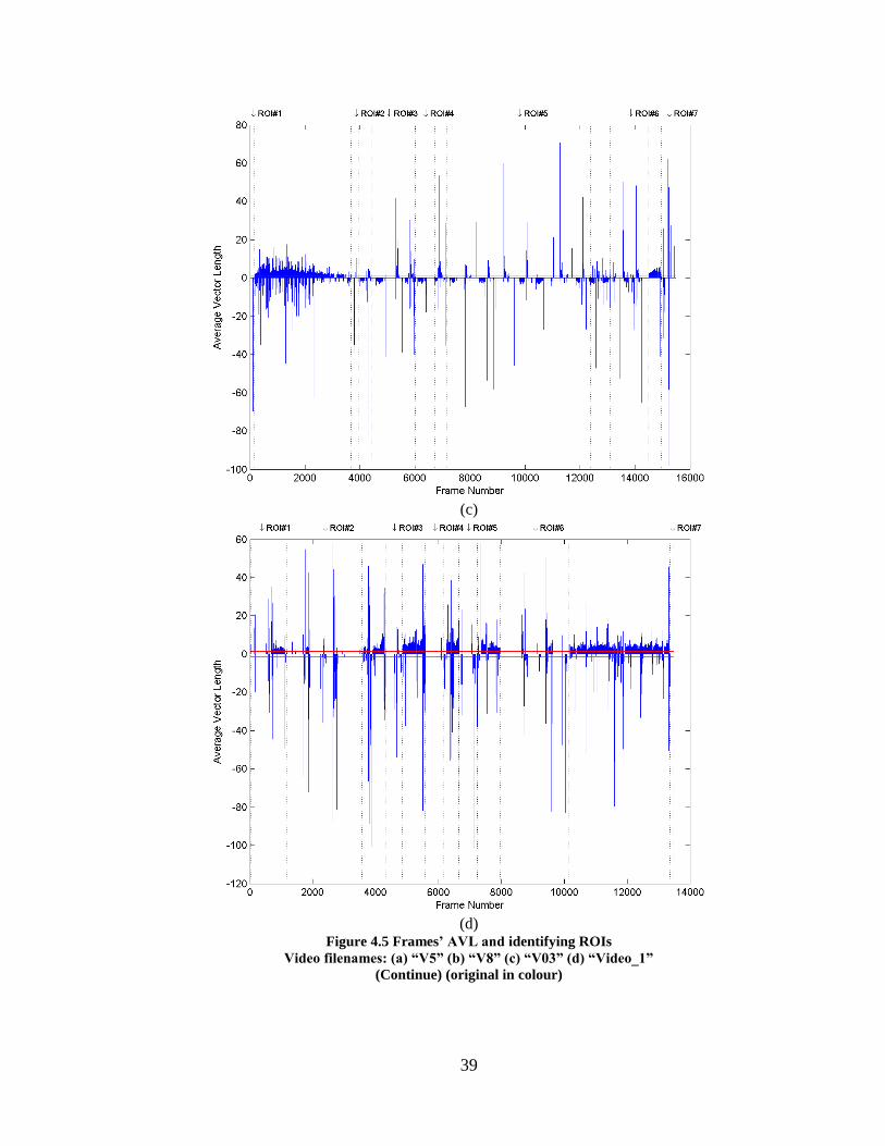
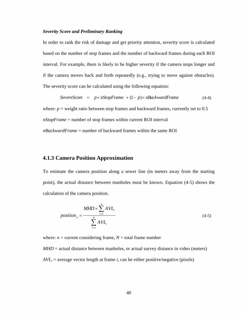
Figure 4.5 Frames’ AVL and identifying ROIs
Video filenames: (a) “V5” (b) “V8” (c) “V03” (d) “Video_1”
(red lines are the ± threshold value) (original in colour)
39
(c)
(d)
Figure 4.5 Frames’ AVL and identifying ROIs
Video filenames: (a) “V5” (b) “V8” (c) “V03” (d) “Video_1”
(Continue) (original in colour)
40
Severity Score and Preliminary Ranking
In order to rank the risk of damage and get priority attention, severity score is calculated
based on the number of stop frames and the number of backward frames during each ROI
interval. For example, there is likely to be higher severity if the camera stops longer and
if the camera moves back and forth repeatedly (e.g., trying to move against obstacles).
The severity score can be calculated using the following equation:
ramenBackwardFpnStopFramepeSevereScor )1( (4-4)
where: p = weight ratio between stop frames and backward frames, currently set to 0.5
nStopFrame = number of stop frames within current ROI interval
nBackwardFrame = number of backward frames within the same ROI
4.1.3 Camera Position Approximation
To estimate the camera position along a sewer line (in meters away from the starting
point), the actual distance between manholes must be known. Equation (4-5) shows the
calculation of the camera position.
N
i
i
n
i
i
n
AVL
AVLMHD
position
1
1 (4-5)
where: n = current considering frame, N = total frame number
MHD = actual distance between manholes, or actual survey distance in video (meters)
AVLi = average vector length at frame i, can be either positive/negative (pixels)

41
For more accuracy, AVL of frames inside identified ROIs should be excluded from the
cumulative vector length (
n
i
iAVL1
). In other words, AVL at ROI frames should be
overwritten with zero value before position computation.
The reason for this is that false distance could be adding up from tilting or circle-like
motions with no actual travelling distance of the camera. OFVs from tilting motion can
produce distance errors with unpredictable direction signs. This means, for example,
rotating clockwise followed by counter clockwise is not always, and not close to, a sum
of zero distance. ROI periods have a high chance of tilting activity; therefore, excluding
AVL during ROIs could reduce error. However, tilting outside ROIs, if it happens, can
still be a problem. Our current work is not able to identify tilting motion, but it will be
considered in future improvements.
42
Figure 4.6 Schematic overview of frame classification
Haar features extraction
Collect FFV, TV, WFV & INFO
sample images
SVMmult learning
SVM model
Learning process (one time)
Frame classes: (1)FFV (2)TV
(3)WFV (4)INFO
SVMmult classification
B&W Image
Median filter
Compute integral image
Haar feature vector
Divide to sub-
windows
Haar features extraction
Use 4 Haar bases to cal.
feature
43
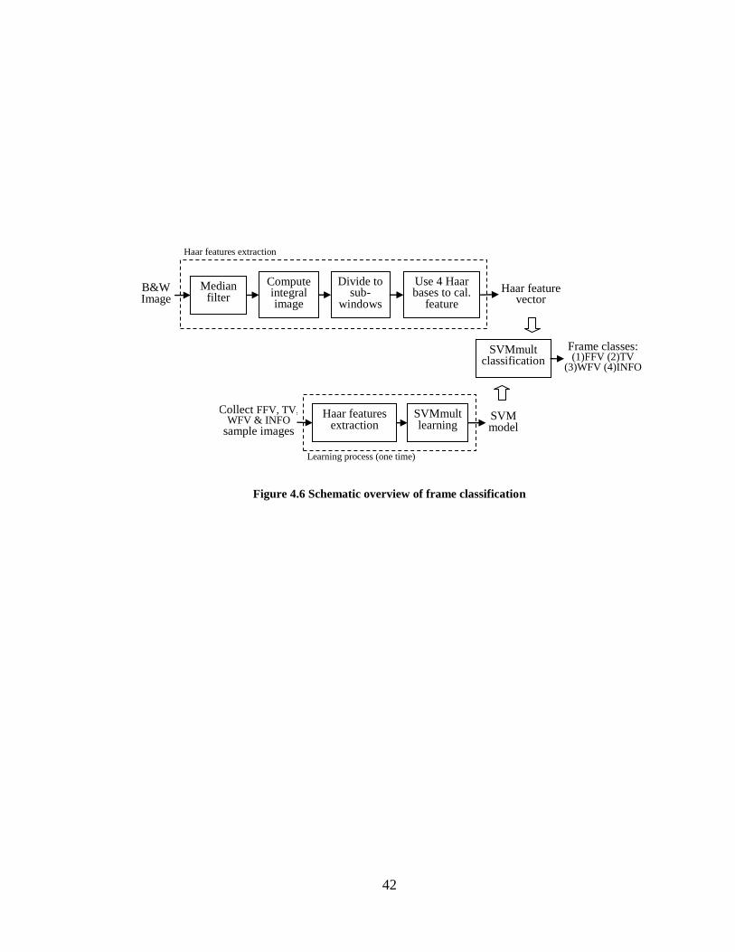
4.2 Sewer Frame Classification and Segmentation
This section describes techniques used to classify sewer frames into categories based on
camera orientation. Different categories apply to different processes and reveal different
defects. The segmentation process only applies for forward-facing view (FFV) frames
and is a prerequisite for the debris detection and the displaced joint detection.
Segmentation includes locating the EOS, estimating flow line, and segmenting wall-water
regions. Information label boxes for detection and removal, which can be used to avoid
false detection of cracks and debris, are also explained here.
4.2.1 Frame Classification
Frame classification is required to reduce the error in and complexity of the defect
detection process. For each ROI, we need to classify every frame into four categories,
which are:
1. Forward-Facing View (FFV) frames – composed of the EOS, wall, and water.
These frames are captured when the camera is pointing toward the EOS.
2. Tilted View (TV) frames – composed of the EOS, wall, and water in an
orientation other than horizontal.
3. Wall-Facing View (WFV) frames – consist of sewer wall only. These frames are
captured when the camera is focusing on suspicious defects on the wall.
4. Information (INFO) frames – the majority of frames consist of information labels
(big rectangular boxes displaying the sewer’s location and other information at the
beginning and/or end of CCTV videos).
44
For minimum complexity, frames in the FFV category will be processed for the following
detection: debris, root, and joint displacement. WFV frames will be only processed for
crack detection. All TV and INFO frames will be ignored. Figure 4.6 shows the
schematic overview of frame classification algorithm.
Image Features Extraction, Training, and Classification
The steps below are followed to extract features from sewer frames. Refer to Section 2.3
in Chapter 2 for review and explanation of how integral image and Haar wavelet features
can be computed.
1. Convert to binary image, then apply median filter
2. Generate integral image for rapid feature extraction, according to Viola and Jones
[35]
3. Divide frame to 5x5 non-overlapping rectangular sub-windows
4. For each sub-window, wavelet features are computed using the 4 bases shown in
Figure 2.1
5. One image should produce a total of (5x5x4) = 100 features
Features extracted from around 400 samples per class were collected, saved to a text file,
and used for training in SVM multiclass learning. FFV frames, TV frames, WFV frames,
and INFO frames data sets are labeled as classes 1, 2, 3, and 4, respectively. A model file
is created when the training process is completed. Figure 4.7 shows examples of FFV
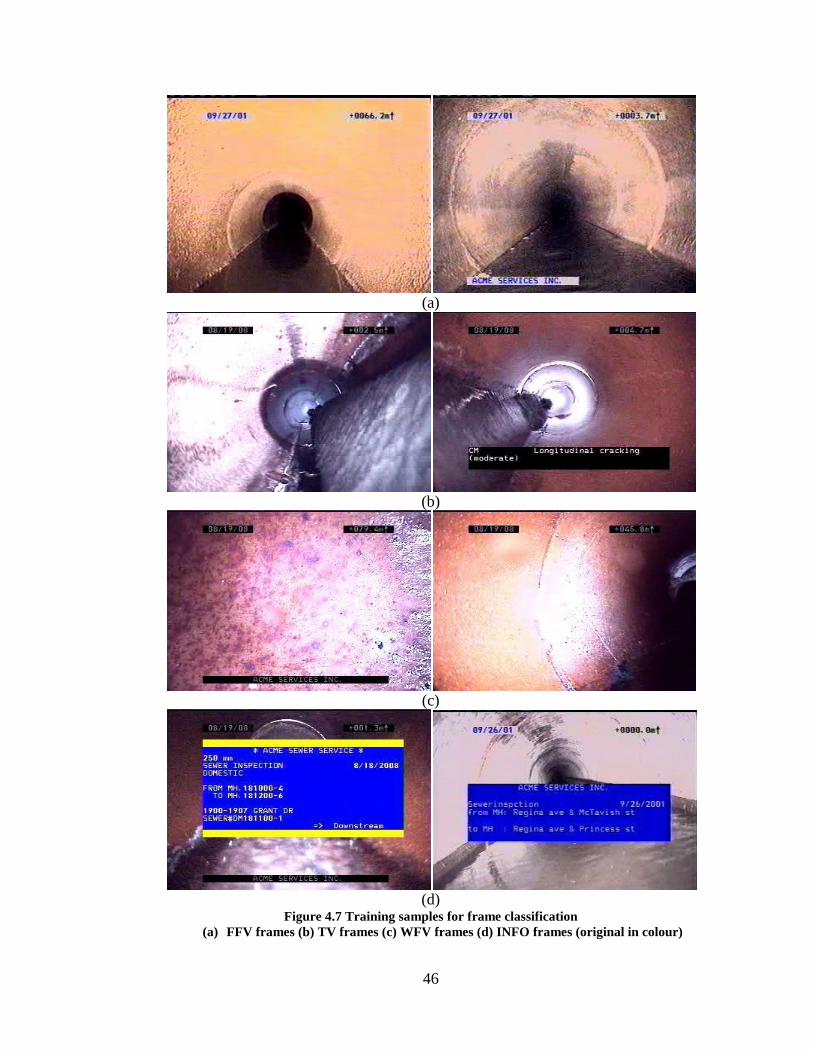
frames, TV frames, WFV frames, and INFO frames that were used for SVM learning.
45
To classify a frame in question, 100 features are computed, similar to when extracting
features for training. Support vectors are obtained from the SVM model file, and then, the
classification score is calculated to categorize the frame type.
Kernel Selection
We constructed a test on 100 samples each of FFV frames, TV frame, and WFV frames,
and 50 samples of INFO frames using different kernels of SVM multiclass classification4.
Table 4.1, Table 4.2, and Table 4.3 show confusion matrices of frame classification by
linear, polynomial 2nd
degree, and radial basis function (RBF), respectively. RBF kernel
gave the best accuracy of 96.86%. Linear kernel is also acceptable with 85.71% accuracy,
while polynomial gave the worst performance of 79.71% accuracy. Therefore, SVM
multiclass with RBF kernel was selected for our frame classification process.
4 Note that all SVM multiclass parameters were set to default values, which are G (gamma) = 1.0 and C
(trade off) = 0.01.
46
(a)
(b)
(c)
(d)
Figure 4.7 Training samples for frame classification
(a) FFV frames (b) TV frames (c) WFV frames (d) INFO frames (original in colour)

47
Table 4.1 Confusion matrix of frame classification by SVM Linear
SVM
Linear
Predicted Total
FFV TV WFV INFO
Act
ual
FFV 78 2 17 3 100
TV 6 81 13 0 100
WFV 7 1 92 0 100
INFO 0 0 1 49 50
Total 91 84 123 52 350
Accuracy = 85.71%
Table 4.2 Confusion matrix of frame classification by SVM Poly2
SVM
Poly2
Predicted Total
FFV TV WFV INFO
Act
ual
FFV 79 0 19 2 100
TV 12 61 26 1 100
WFV 4 0 96 0 100
INFO 0 0 7 43 50
Total 95 61 148 46 350
Accuracy = 79.71%
Table 4.3 Confusion matrix of frame classification by SVM RBF
SVM
RBF
Predicted Total
FFV TV WFV INFO
Act
ual
FFV 94 1 3 2 100
TV 2 96 1 1 100
WFV 1 0 99 0 100
INFO 0 0 0 50 50
Total 97 97 103 53 350
Accuracy = 96.86%
48
Figure 4.8 Schematic overview of EOS location search and verification
Greyscale
Image (FFV)
Plot avg. horizontal
grey intensity
Determine frame type from plot’s
shape
EOS center on x-axis = min peak position
EOS center
Verify by
circle
intensity
subtraction Plot avg.
vertical grey
intensity
(if dark)
(if bright)
EOS center on x-axis = max peak position
Plot grey intensity along ver. line at EOS center (x-axis)
EOS center on y-axis = min peak position
EOS center on y-axis = max peak position
49
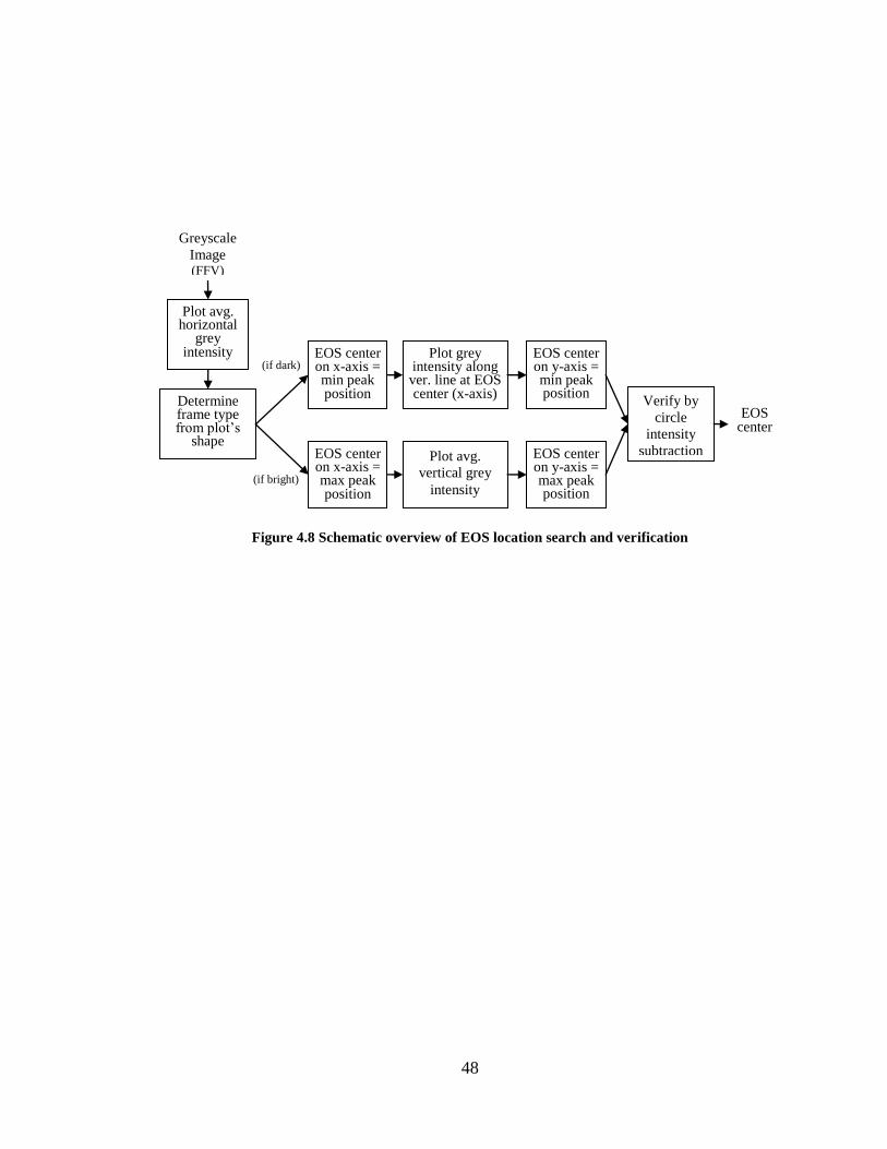
4.2.2 EOS Location Search and Verification
Refer to the schematic shown in Figure 4.8, the first step of locating the end-of-sewer
(EOS) is to differentiate FFV frames between two types: dark EOS and bright EOS5, see
Figure 4.9, unless the user sets EOS type to either “dark” or “bright.” The steps to locate
the EOS center are given below. Note that small areas around frame edges are always
excluded from the intensity plot to avoid error caused by information label boxes and, in
some cases, irregular intensity close to edges.
1. Convert a frame to greyscale and plot the average grey intensity along the
horizontal axis, excluding small areas close to the left and right edges.
2. Determine if the EOS is dark or bright6. By computing its slope, it is a dark EOS
frame if the plot is trending to an upward U-shape similar to Figure 4.10(a);
otherwise, it is a bright EOS frame if the plot has a downward U-shape as in
Figure 4.10(b).
3. Smooth the intensity plot by moving the average in order to allow the peak
detection to deal with the trend of the plot, instead of noisy data, to avoid local
peak errors.
4. Detect the minimum peak of the smoothed plot for a dark EOS or the maximum
peak of the smoothed plot for a white EOS to locate the position of the EOS
center on the x-axis, refer to Figure 4.10.
5. To locate the position of the EOS on y-axis:
5 Bright EOS occurred from light reflection of the camera to the sewer cleaning unit, when injecting water
to clean sewer wall. 6 This step will be skipped if the user defines EOS type as either “dark” or “bright” (default set to auto
determination) in the options setting, see Chapter 3.
50
For a dark EOS, plot and smooth the grey value along a column at the x-
position obtained from the previous step (i.e., along the vertical line in Figure
4.10(c)), but exclude small areas close to the upper and lower edges. The
minimum point of the plot, see Figure 4.11(a), yields the location of the EOS
center on the y-axis.
For a bright EOS, plot and smooth the average grey intensity along the y-axis,
ignoring small areas close to the upper and lower edges. The maximum peak
on the plot, see Figure 4.11(b), is the location of the EOS center on the y-axis.
NOTE: Using average grey value yields greater accuracy than plotting the grey
pixel value along a column (vertical line) directly because averaging the plot is
independent from the pre-located position of the EOS on the x-axis. However,
averaging the grey value for the dark EOS frame will not work because there will
be no significant jump on the plot; therefore, direct plotting of the grey pixels
along the vertical line is more suitable for sewer frames with dark EOSs, and
averaging the plot is best for frames with bright EOSs.
6. This is an extra step to get more precise locations, but it is applicable for dark
EOSs only. Some irregular bright or dark spots on the wall could produce false
peaks on the plot. Therefore, detecting EOS location in smaller regions can reduce
noise effects in the intensity plot.
Crop a sub-window centering at the EOS location from the first run
Repeat steps 4 and 5 to adjust EOS location
If not successful, crop a bigger sub-window and repeat steps 4 and 5 again
until a new location is found.

51
(a)
(b)
Figure 4.9 Frames with dark and bright EOS (original in colour)
(a)
(b)
(c)
(d)
Figure 4.10 Locating EOS position on x-axis
(a) and (b) show average grey intensity plots for dark and bright EOS
(c) show detected EOS center line on x-axis at 133 for dark (d) at 173 for bright EOS frame (original
in colour)

52
EOS Location Verification
The EOS location is verified to be present at the predicted location. Due to the fact that
the EOS and wall have difference grey intensities, we can verify the EOS by the
following steps:
1. Draw 2 circles: Draw an inner circle and outer circle around the predicted EOS
center, see Figure 4.12. The base radii for dark EOSs are equal to 20 pixels (inner
circle) and 60 pixels (outer circle). The radii for bright EOSs are 50 pixels and
100 pixels.
2. Calculate average pixel values of the region inside the inner circle and the region
between the inner and outer circles.
3. EOS is valid if the difference between the average intensity of the EOS region
(inside inner circle) and the surrounding area (between inner and outer circle) is
greater than a predefined threshold value, which can be obtained by trial and
error. The threshold currently used is 48 for dark EOSs and 40 for bright EOSs.
Failed verification means 1) the frame does not belong to the FFV category or 2) the
predicted location is misplaced.
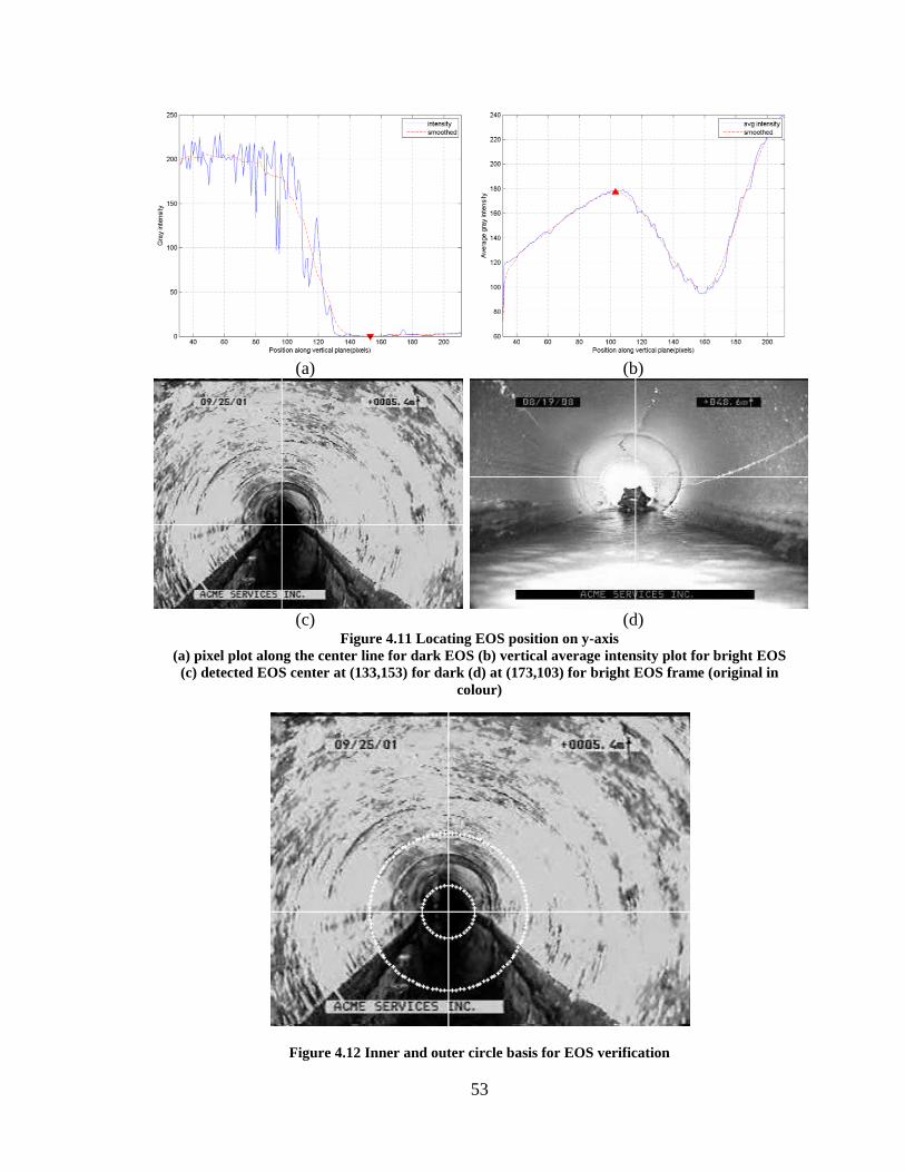
53
(a)
(b)
(c)
(d)
Figure 4.11 Locating EOS position on y-axis
(a) pixel plot along the center line for dark EOS (b) vertical average intensity plot for bright EOS
(c) detected EOS center at (133,153) for dark (d) at (173,103) for bright EOS frame (original in
colour)
Figure 4.12 Inner and outer circle basis for EOS verification
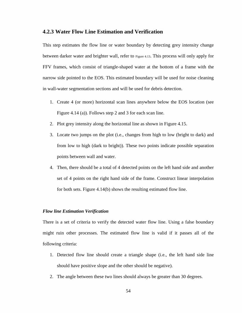
54
4.2.3 Water Flow Line Estimation and Verification
This step estimates the flow line or water boundary by detecting grey intensity change
between darker water and brighter wall, refer to Figure 4.13. This process will only apply for
FFV frames, which consist of triangle-shaped water at the bottom of a frame with the
narrow side pointed to the EOS. This estimated boundary will be used for noise cleaning
in wall-water segmentation sections and will be used for debris detection.
1. Create 4 (or more) horizontal scan lines anywhere below the EOS location (see
Figure 4.14 (a)). Follows step 2 and 3 for each scan line.
2. Plot grey intensity along the horizontal line as shown in Figure 4.15.
3. Locate two jumps on the plot (i.e., changes from high to low (bright to dark) and
from low to high (dark to bright)). These two points indicate possible separation
points between wall and water.
4. Then, there should be a total of 4 detected points on the left hand side and another
set of 4 points on the right hand side of the frame. Construct linear interpolation
for both sets. Figure 4.14(b) shows the resulting estimated flow line.
Flow line Estimation Verification
There is a set of criteria to verify the detected water flow line. Using a false boundary
might ruin other processes. The estimated flow line is valid if it passes all of the
following criteria:
1. Detected flow line should create a triangle shape (i.e., the left hand side line
should have positive slope and the other should be negative).
2. The angle between these two lines should always be greater than 30 degrees.

55
Figure 4.13 Schematic overview of water flow line estimation and verification
(a)
(b)
Figure 4.14 Flow line estimation
(a) horizontal scan lines (b) final water boundary
Figure 4.15 Grey intensity plotting along one horizontal scan line
(red-vertical lines show detected intensity jump) (original in colour)
Greyscale Image (FFV)
Create horizontal scan lines
Water flow line
Plot grey intensity along each scan line
Detect intensity jumps of each
plot
Linear interpolation of detected points
Verify valid
flow line
detected
jump
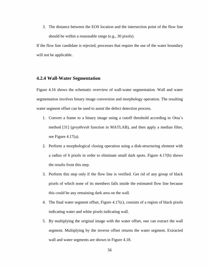
56
3. The distance between the EOS location and the intersection point of the flow line
should be within a reasonable range (e.g., 30 pixels).
If the flow line candidate is rejected, processes that require the use of the water boundary
will not be applicable.
4.2.4 Wall-Water Segmentation
Figure 4.16 shows the schematic overview of wall-water segmentation. Wall and water
segmentation involves binary image conversion and morphology operation. The resulting
water segment offset can be used to assist the defect detection process.
1. Convert a frame to a binary image using a cutoff threshold according to Otsu`s
method [31] (greythresh function in MATLAB), and then apply a median filter,
see Figure 4.17(a).
2. Perform a morphological closing operation using a disk-structuring element with
a radius of 6 pixels in order to eliminate small dark spots. Figure 4.17(b) shows
the results from this step.
3. Perform this step only if the flow line is verified. Get rid of any group of black
pixels of which none of its members falls inside the estimated flow line because
this could be any remaining dark area on the wall.
4. The final water segment offset, Figure 4.17(c), consists of a region of black pixels
indicating water and white pixels indicating wall.
5. By multiplying the original image with the water offset, one can extract the wall
segment. Multiplying by the inverse offset returns the water segment. Extracted
wall and water segments are shown in Figure 4.18.
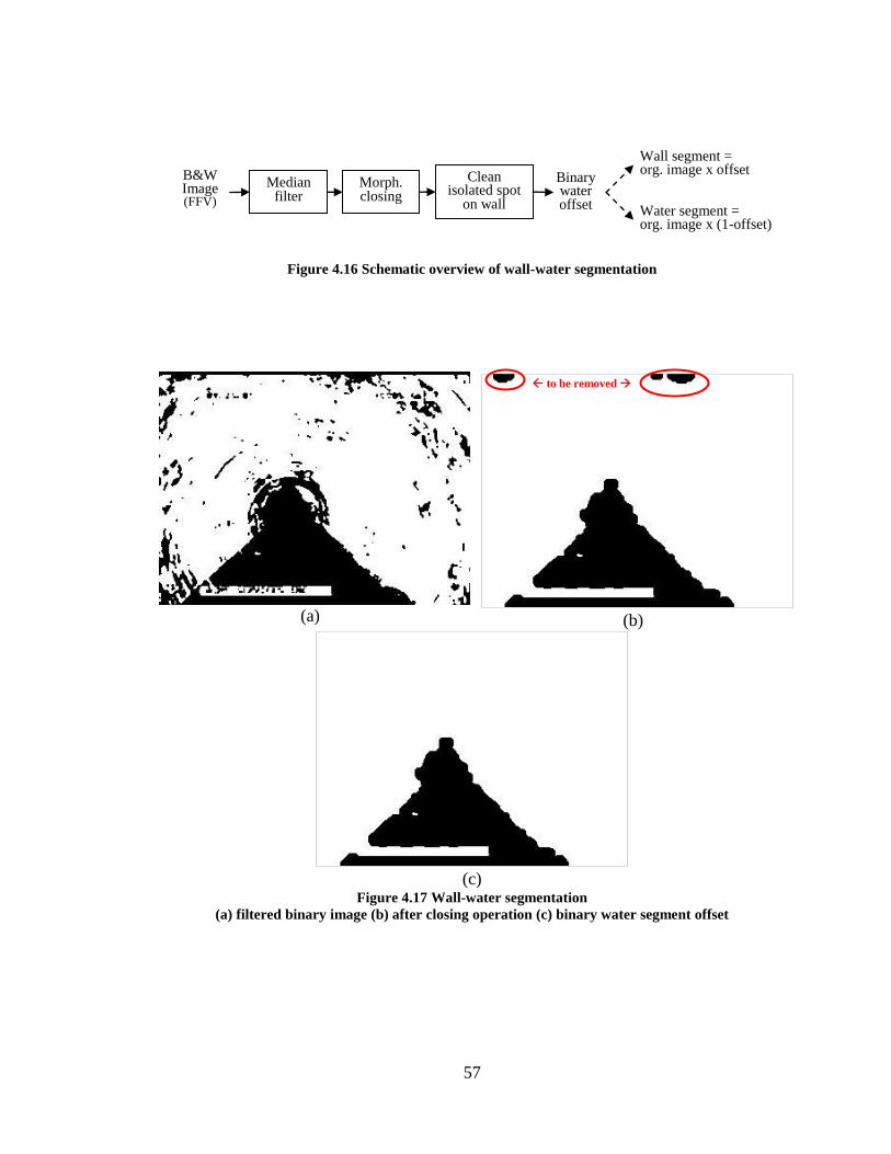
57
Figure 4.16 Schematic overview of wall-water segmentation
(a)
(b)
(c)
Figure 4.17 Wall-water segmentation
(a) filtered binary image (b) after closing operation (c) binary water segment offset
B&W Image (FFV)
Median filter
Binary water offset
Morph. closing
Clean isolated spot
on wall
Wall segment = org. image x offset
Water segment = org. image x (1-offset)
to be removed
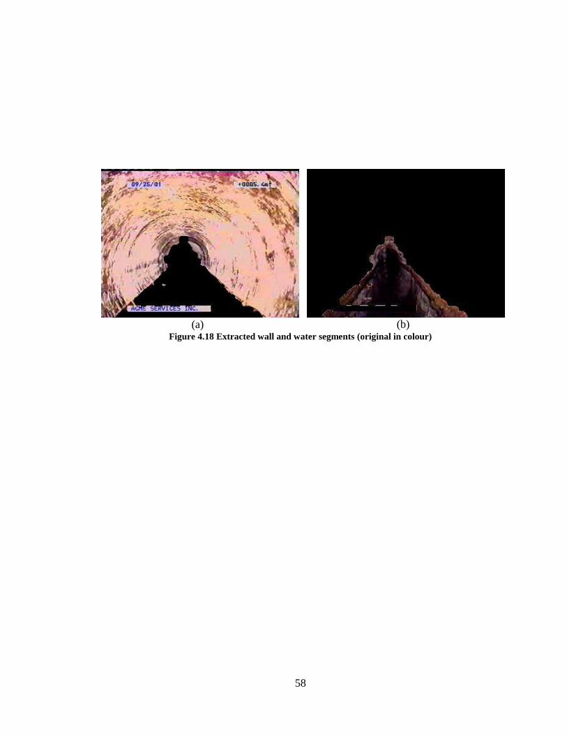
58
(a)
(b)
Figure 4.18 Extracted wall and water segments (original in colour)
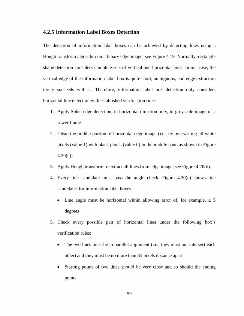
59
4.2.5 Information Label Boxes Detection
The detection of information label boxes can be achieved by detecting lines using a
Hough transform algorithm on a binary edge image, see Figure 4.19. Normally, rectangle
shape detection considers complete sets of vertical and horizontal lines. In our case, the
vertical edge of the information label box is quite short, ambiguous, and edge extraction
rarely succeeds with it. Therefore, information label box detection only considers
horizontal line detection with established verification rules.
1. Apply Sobel edge detection, in horizontal direction only, to greyscale image of a
sewer frame
2. Clean the middle portion of horizontal edge image (i.e., by overwriting all white
pixels (value 1) with black pixels (value 0) in the middle band as shown in Figure
4.20(c))
3. Apply Hough transform to extract all lines from edge image, see Figure 4.20(d).
4. Every line candidate must pass the angle check. Figure 4.20(e) shows line
candidates for information label boxes.
Line angle must be horizontal within allowing error of, for example, ± 5
degrees
5. Check every possible pair of horizontal lines under the following box’s
verification rules:
The two lines must be in parallel alignment (i.e., they must not intersect each
other) and they must be no more than 35 pixels distance apart
Starting points of two lines should be very close and so should the ending
points
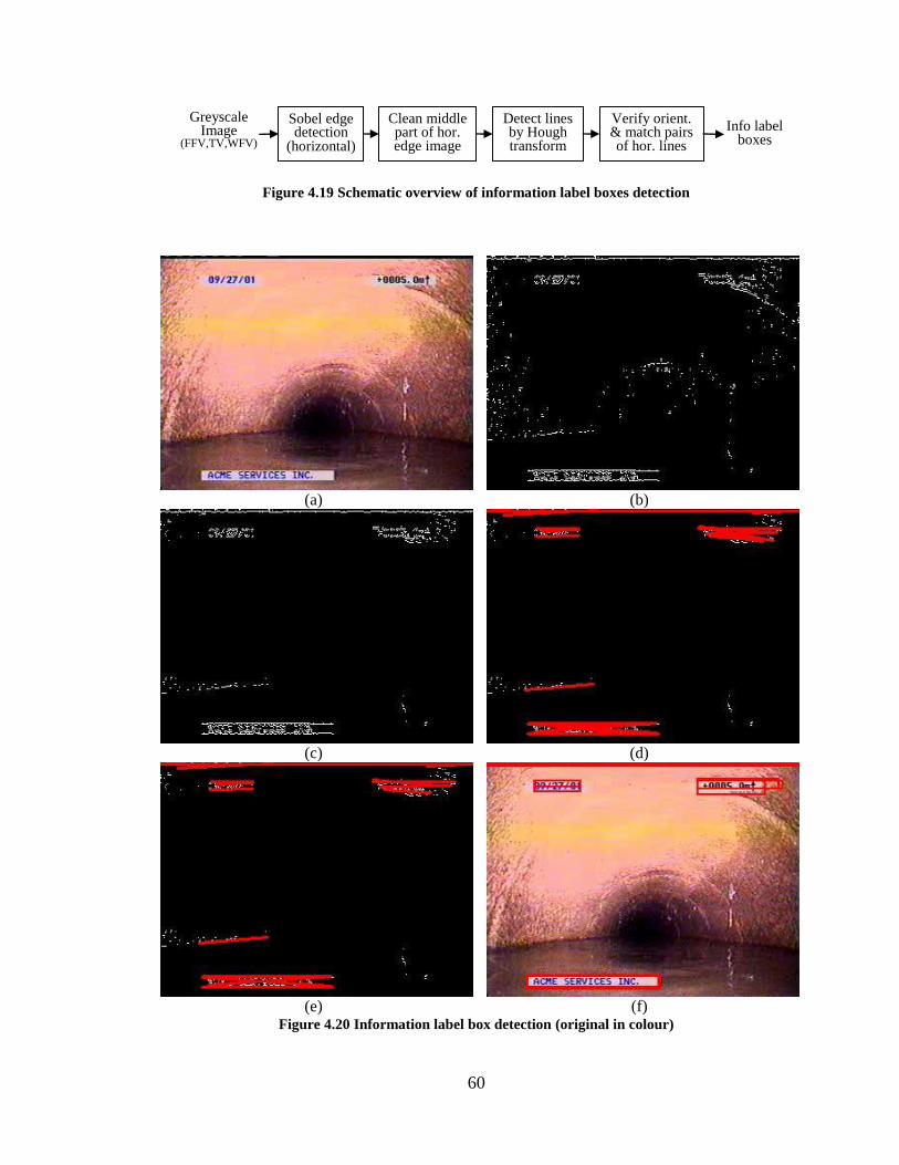
60
Figure 4.19 Schematic overview of information label boxes detection
(a)
(b)
(c)
(d)
(e)
(f)
Figure 4.20 Information label box detection (original in colour)
Greyscale Image
(FFV,TV,WFV)
Sobel edge detection
(horizontal)
Info label boxes
Clean middle part of hor. edge image
Detect lines by Hough transform
Verify orient. & match pairs of hor. lines
61
6. Each pair that satisfies verification rules is considered as a rectangular box, see
Figure 4.20(f). All pixels inside these detected boxes can be now removed as
needed.
4.3 Defect Detection Algorithms
This section explains the algorithms used to detect sewer structural (i.e. crack, joint) and
operational defects (i.e., debris, roots) from CCTV images. Frames are processed for
defect detection according to their categories (i.e., FFV for debris, roots, and joints, and
WFV for cracks).
4.3.1 Debris Detection
Suspicious debris or waste on the water surface can be detected by identifying any object
in the water region. However, there are many false positives such as shadows and bright
water areas due to reflection of the camera’s light. Therefore, a post-process is required to
reduce false positives. Note that the difference between debris and non-debris regions is
the complexity of their surfaces. Non-debris surface is normally smoother compared to
debris surface. As a result, texture analysis should be one of the most suitable methods to
measure texture-context information and reject smooth surface area. Figure 4.21 shows
the overview of debris detection algorithm.
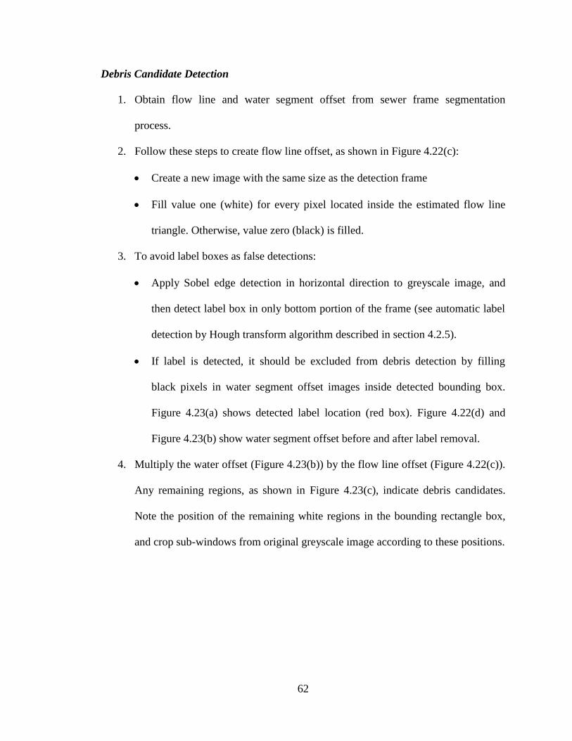
62
Debris Candidate Detection
1. Obtain flow line and water segment offset from sewer frame segmentation
process.
2. Follow these steps to create flow line offset, as shown in Figure 4.22(c):
Create a new image with the same size as the detection frame
Fill value one (white) for every pixel located inside the estimated flow line
triangle. Otherwise, value zero (black) is filled.
3. To avoid label boxes as false detections:
Apply Sobel edge detection in horizontal direction to greyscale image, and
then detect label box in only bottom portion of the frame (see automatic label
detection by Hough transform algorithm described in section 4.2.5).
If label is detected, it should be excluded from debris detection by filling
black pixels in water segment offset images inside detected bounding box.
Figure 4.23(a) shows detected label location (red box). Figure 4.22(d) and
Figure 4.23(b) show water segment offset before and after label removal.
4. Multiply the water offset (Figure 4.23(b)) by the flow line offset (Figure 4.22(c)).
Any remaining regions, as shown in Figure 4.23(c), indicate debris candidates.
Note the position of the remaining white regions in the bounding rectangle box,
and crop sub-windows from original greyscale image according to these positions.
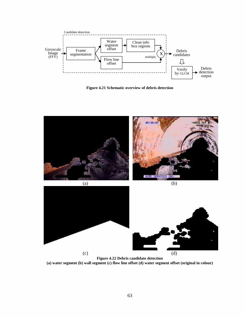
63
Figure 4.21 Schematic overview of debris detection
(a)
(b)
(c)
(d)
Figure 4.22 Debris candidate detection
(a) water segment (b) wall segment (c) flow line offset (d) water segment offset (original in colour)
Greyscale Image (FFV)
Frame segmentation
Flow line offset
Water segment
offset
Clean info box regions
Debris detection
output
X multiply
Debris candidates
Verify by GLCM
Candidate detection
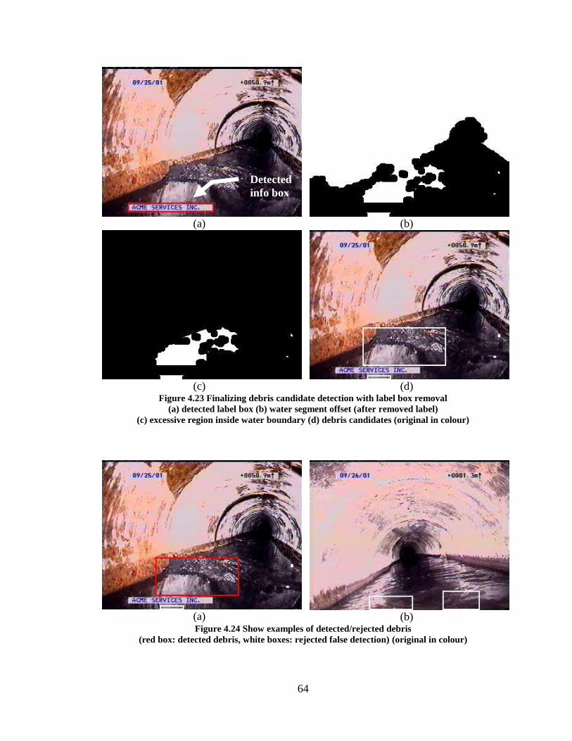
64
(a)
(b)
(c)
(d)
Figure 4.23 Finalizing debris candidate detection with label box removal
(a) detected label box (b) water segment offset (after removed label)
(c) excessive region inside water boundary (d) debris candidates (original in colour)
(a)
(b)
Figure 4.24 Show examples of detected/rejected debris
(red box: detected debris, white boxes: rejected false detection) (original in colour)
Detected
info box

65
Debris Candidate Verification by Texture Analysis
Debris and non-debris candidates can be differentiated by assessing texture
characteristics or the roughness of their surface. GLCM’s entropy feature, which is the
most commonly used feature [6], was selected. Entropy measures the randomness of an
image and gives a high score when texture is not uniform. This means smooth water
surface should give low entropy values, and rough debris surface should give high values.
1. For each cropped greyscale rectangle region of suspicious debris, create four
angular (0, 45, 90, and 135) co-occurrence matrices with 32 grey level
quantization, and distance = 1. Normalize each matrix by dividing by the total
number of neighbouring pairs (equivalent to the total sum of the matrix).
2. Calculate the GLCM entropy feature of the four angular matrices using Equation
(4-6). Then, the texture score is equal to the average of these four entropy values.
g
i
g
j
jipjipEntropy1 1
)),(log(),( (4-6)
where: p(i,j) = (i,j) in a normalized co-occurrence matrix
g = number of quantized grey levels
3. Discard regions of which the texture score is less than a specific threshold value;
otherwise, it is a positive detection. For the best result, a threshold value of 4.9
was chosen as discovered by trial and error7. Figure 4.24 shows red boxes for the
detected debris and white boxes for the rejected suspicious regions.
7 The test was set up by collecting a group of clean water surface sub-images and a group of sub-images
with debris. Values between the average texture score of the water surface group and average texture score
of the debris group were randomly selected and, then, tested against another set of water surface sub-
images and debris sub-images. The threshold value that gave the highest performance was 4.9.
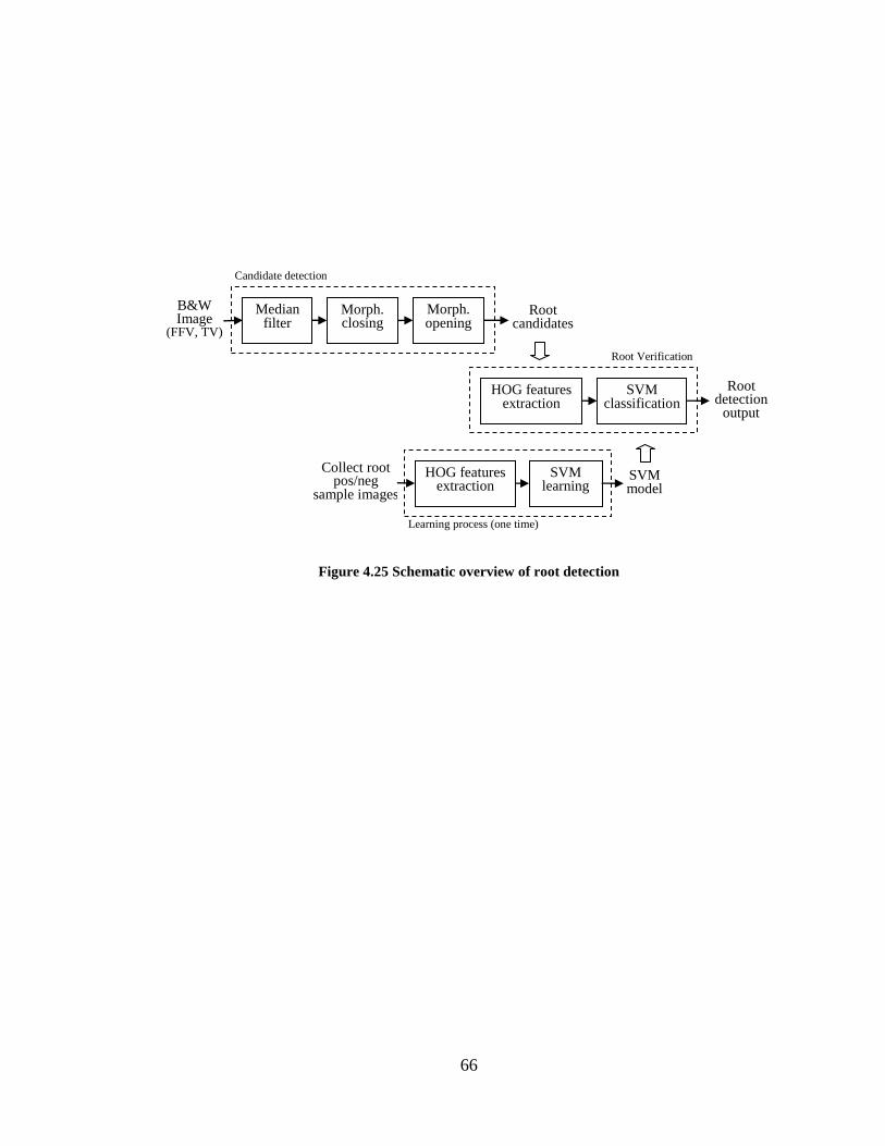
66
Figure 4.25 Schematic overview of root detection
B&W Image
(FFV, TV)
Median filter
Morph. closing
Root candidates
Morph. opening
Candidate detection
HOG features extraction
Collect root pos/neg
sample images
SVM learning
SVM model
Learning process (one time)
Root detection
output
HOG features extraction
SVM classification
Root Verification
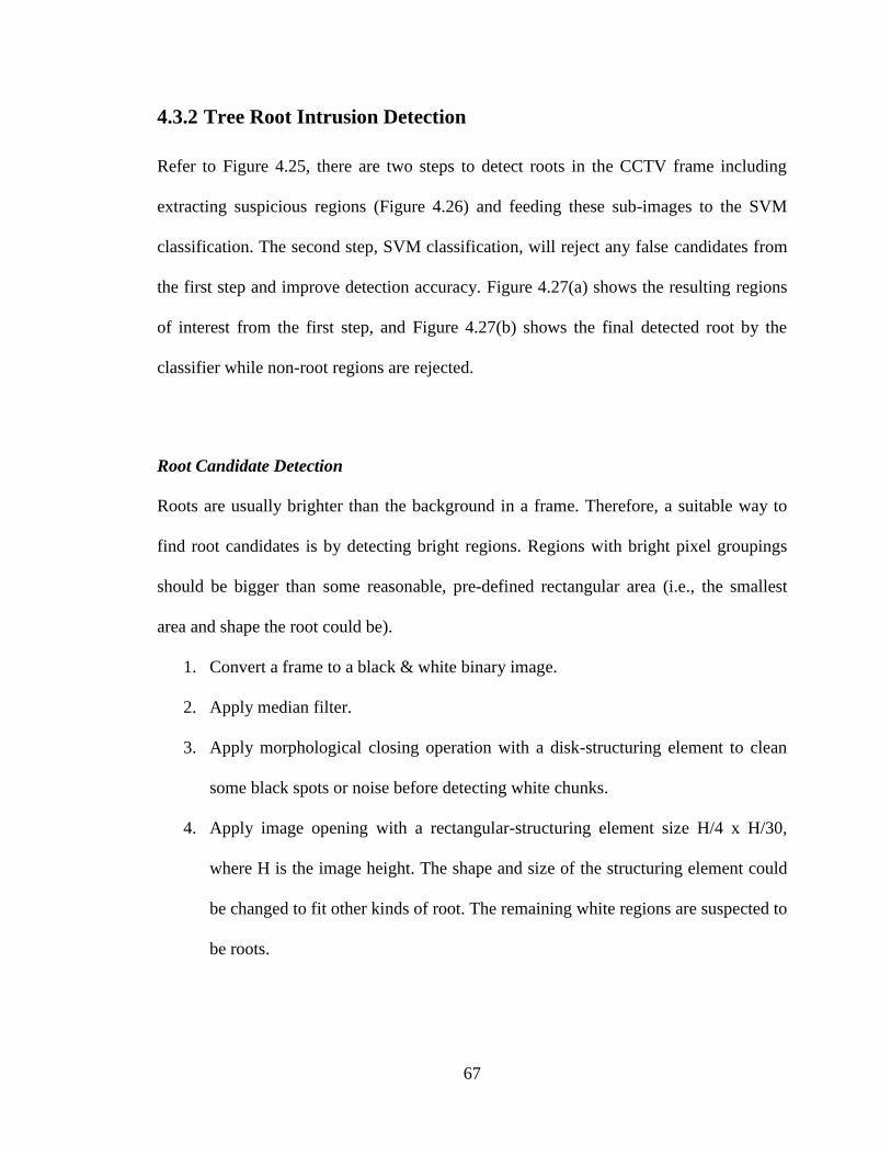
67
4.3.2 Tree Root Intrusion Detection
Refer to Figure 4.25, there are two steps to detect roots in the CCTV frame including
extracting suspicious regions (Figure 4.26) and feeding these sub-images to the SVM
classification. The second step, SVM classification, will reject any false candidates from
the first step and improve detection accuracy. Figure 4.27(a) shows the resulting regions
of interest from the first step, and Figure 4.27(b) shows the final detected root by the
classifier while non-root regions are rejected.
Root Candidate Detection
Roots are usually brighter than the background in a frame. Therefore, a suitable way to
find root candidates is by detecting bright regions. Regions with bright pixel groupings
should be bigger than some reasonable, pre-defined rectangular area (i.e., the smallest
area and shape the root could be).
1. Convert a frame to a black & white binary image.
2. Apply median filter.
3. Apply morphological closing operation with a disk-structuring element to clean
some black spots or noise before detecting white chunks.
4. Apply image opening with a rectangular-structuring element size H/4 x H/30,
where H is the image height. The shape and size of the structuring element could
be changed to fit other kinds of root. The remaining white regions are suspected to
be roots.
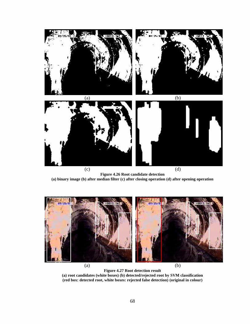
68
(a)
(b)
(c)
(d)
Figure 4.26 Root candidate detection
(a) binary image (b) after median filter (c) after closing operation (d) after opening operation
(a)
(b)
Figure 4.27 Root detection result
(a) root candidates (white boxes) (b) detected/rejected root by SVM classification
(red box: detected root, white boxes: rejected false detection) (original in colour)

69
5. Record the bounding box positions of white regions as in Figure 4.26(d). Figure
4.27(a) shows the drawing of regions of interest on the original image. These
rectangular sub-regions will be used again in the root recognition section.
Root Candidate Verification by Image Recognition Technique
Image recognition technique is used to recognize and verify positive detection by using
Histograms of Oriented Gradients (HOGs) [30] and the SVM classification tool [52] with
a Linear kernel.
Follow these steps to extract HOG features from root candidates:
1. Resize each sub-image to 100x100 pixels because suspicious windows usually
come in various sizes
2. Divide the detecting window into non-overlapping small cells and blocks. The
cell size currently used is 10x10 pixels and the block size is 5x5 cells.
3. Calculate and accumulate a local gradient histogram within each cell by
quantizing unsigned gradients into 9 orientation bins.
4. Normalize all cells in a block using L2-norm, see Equation (2-5).
5. There are 9 features per cell, 25 cells per block, and 4 blocks per image; therefore,
there will be a total of (9x25x4) = 900 features per image.
To train the classification model, 500 positive and 500 negative examples were collected,
and HOG features were extracted and then saved to training text files (one line per
example). The positive examples are sub-windows showing root intrusions, and the
negative examples are any randomly cropped areas from ‘no-root-defected’ frames; see
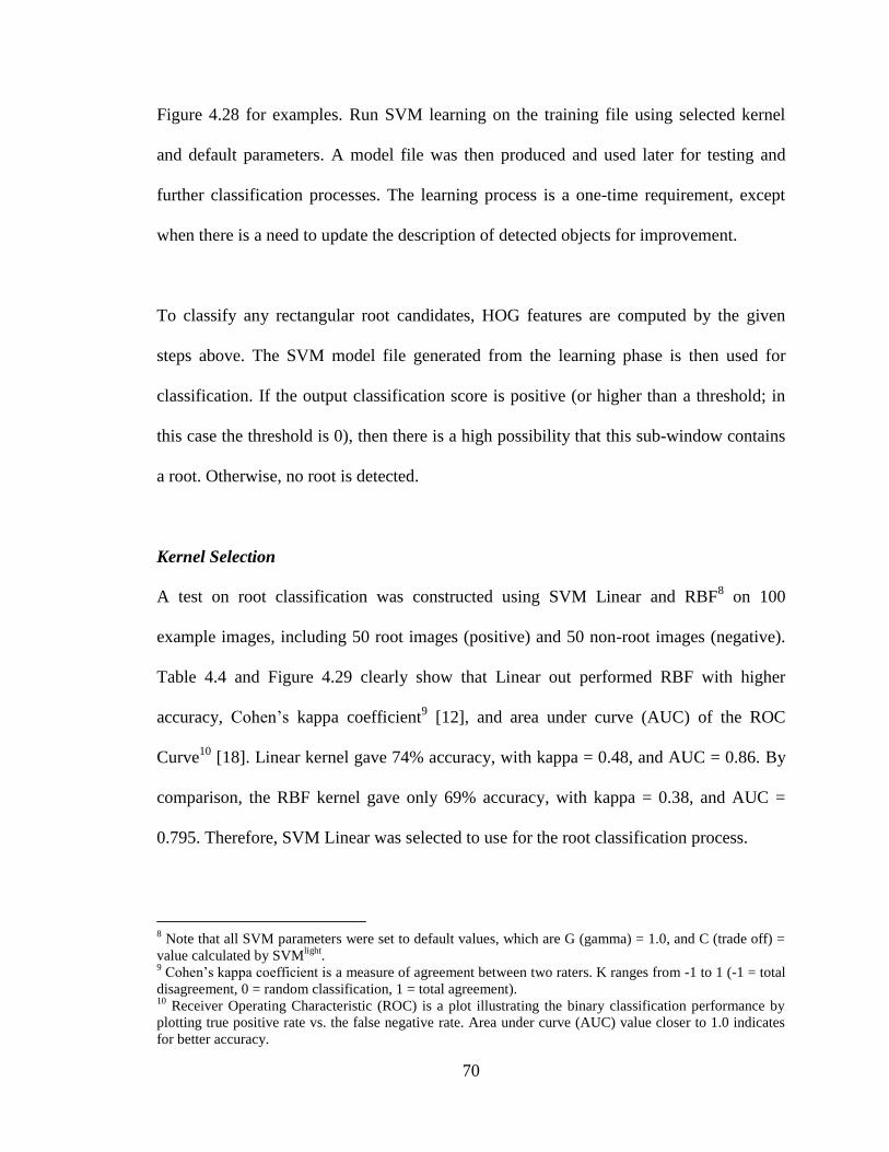
70
Figure 4.28 for examples. Run SVM learning on the training file using selected kernel
and default parameters. A model file was then produced and used later for testing and
further classification processes. The learning process is a one-time requirement, except
when there is a need to update the description of detected objects for improvement.
To classify any rectangular root candidates, HOG features are computed by the given
steps above. The SVM model file generated from the learning phase is then used for
classification. If the output classification score is positive (or higher than a threshold; in
this case the threshold is 0), then there is a high possibility that this sub-window contains
a root. Otherwise, no root is detected.
Kernel Selection
A test on root classification was constructed using SVM Linear and RBF8 on 100
example images, including 50 root images (positive) and 50 non-root images (negative).
Table 4.4 and Figure 4.29 clearly show that Linear out performed RBF with higher
accuracy, Cohen’s kappa coefficient9 [12], and area under curve (AUC) of the ROC
Curve10
[18]. Linear kernel gave 74% accuracy, with kappa = 0.48, and AUC = 0.86. By
comparison, the RBF kernel gave only 69% accuracy, with kappa = 0.38, and AUC =
0.795. Therefore, SVM Linear was selected to use for the root classification process.
8 Note that all SVM parameters were set to default values, which are G (gamma) = 1.0, and C (trade off) =
value calculated by SVMlight
. 9 Cohen’s kappa coefficient is a measure of agreement between two raters. K ranges from -1 to 1 (-1 = total
disagreement, 0 = random classification, 1 = total agreement). 10
Receiver Operating Characteristic (ROC) is a plot illustrating the binary classification performance by
plotting true positive rate vs. the false negative rate. Area under curve (AUC) value closer to 1.0 indicates
for better accuracy.
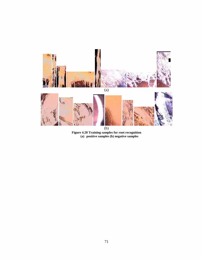
71
(a)
(b)
Figure 4.28 Training samples for root recognition
(a) positive samples (b) negative samples
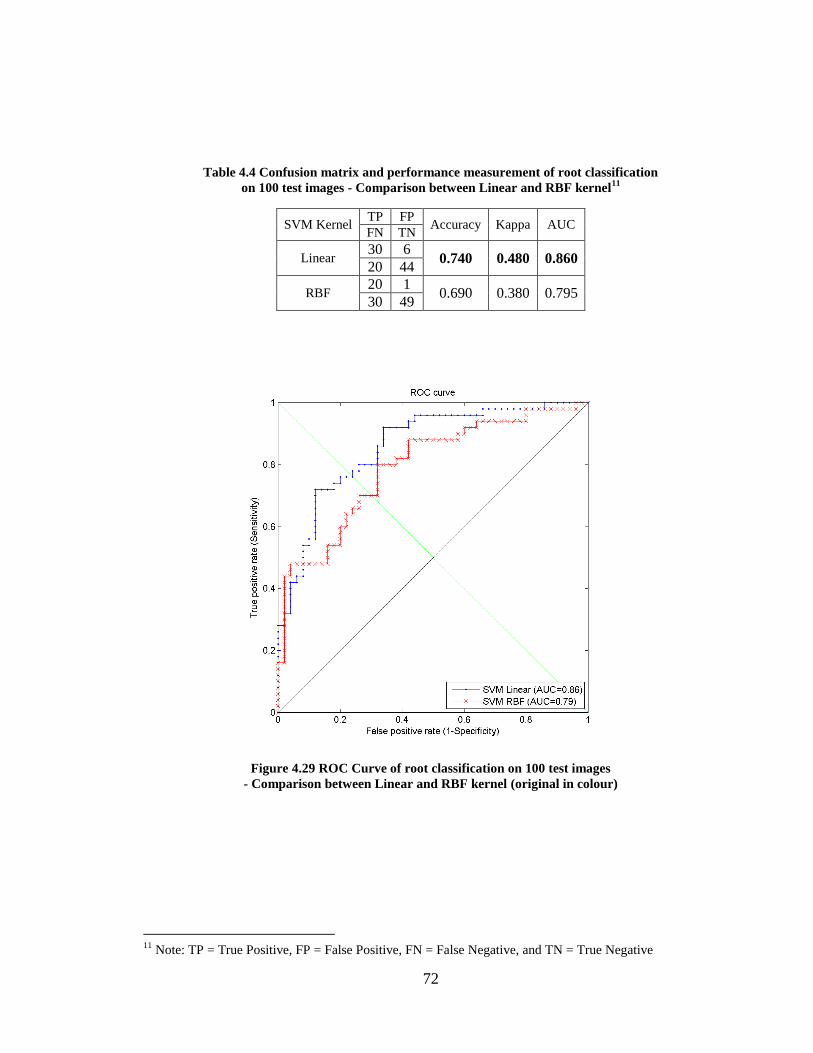
72
Table 4.4 Confusion matrix and performance measurement of root classification
on 100 test images - Comparison between Linear and RBF kernel11
SVM Kernel TP FP
Accuracy Kappa AUC FN TN
Linear 30 6
0.740 0.480 0.860 20 44
RBF 20 1
0.690 0.380 0.795 30 49
Figure 4.29 ROC Curve of root classification on 100 test images
- Comparison between Linear and RBF kernel (original in colour)
11
Note: TP = True Positive, FP = False Positive, FN = False Negative, and TN = True Negative
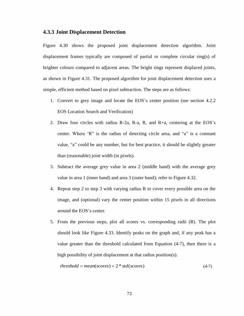
73
4.3.3 Joint Displacement Detection
Figure 4.30 shows the proposed joint displacement detection algorithm. Joint
displacement frames typically are composed of partial or complete circular ring(s) of
brighter colours compared to adjacent areas. The bright rings represent displaced joints,
as shown in Figure 4.31. The proposed algorithm for joint displacement detection uses a
simple, efficient method based on pixel subtraction. The steps are as follows:
1. Convert to grey image and locate the EOS’s center position (see section 4.2.2
EOS Location Search and Verification)
2. Draw four circles with radius R-2a, R-a, R, and R+a, centering at the EOS’s
center. Where ‘R” is the radius of detecting circle area, and “a” is a constant
value, “a” could be any number, but for best practice, it should be slightly greater
than (reasonable) joint width (in pixels).
3. Subtract the average grey value in area 2 (middle band) with the average grey
value in area 1 (inner band) and area 3 (outer band); refer to Figure 4.32.
4. Repeat step 2 to step 3 with varying radius R to cover every possible area on the
image, and (optional) vary the center position within 15 pixels in all directions
around the EOS’s center.
5. From the previous steps, plot all scores vs. corresponding radii (R). The plot
should look like Figure 4.33. Identify peaks on the graph and, if any peak has a
value greater than the threshold calculated from Equation (4-7), then there is a
high possibility of joint displacement at that radius position(s).
)(*2)( scoresstdscoresmeanthreshold (4-7)
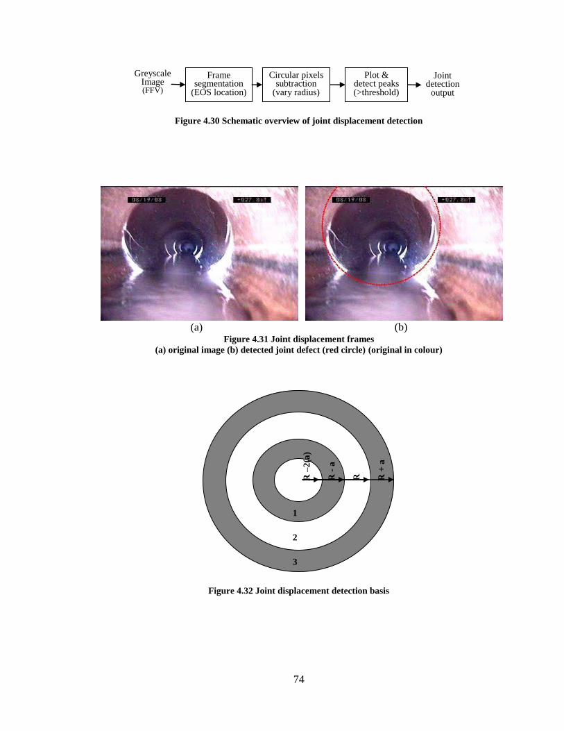
74
Figure 4.30 Schematic overview of joint displacement detection
(a)
(b)
Figure 4.31 Joint displacement frames
(a) original image (b) detected joint defect (red circle) (original in colour)
Figure 4.32 Joint displacement detection basis
1
2
3
R
R -
a
R +
a
R –
2(a
)
Greyscale Image (FFV)
Frame segmentation
(EOS location)
Joint detection
output
Circular pixels subtraction
(vary radius)
Plot & detect peaks (>threshold)
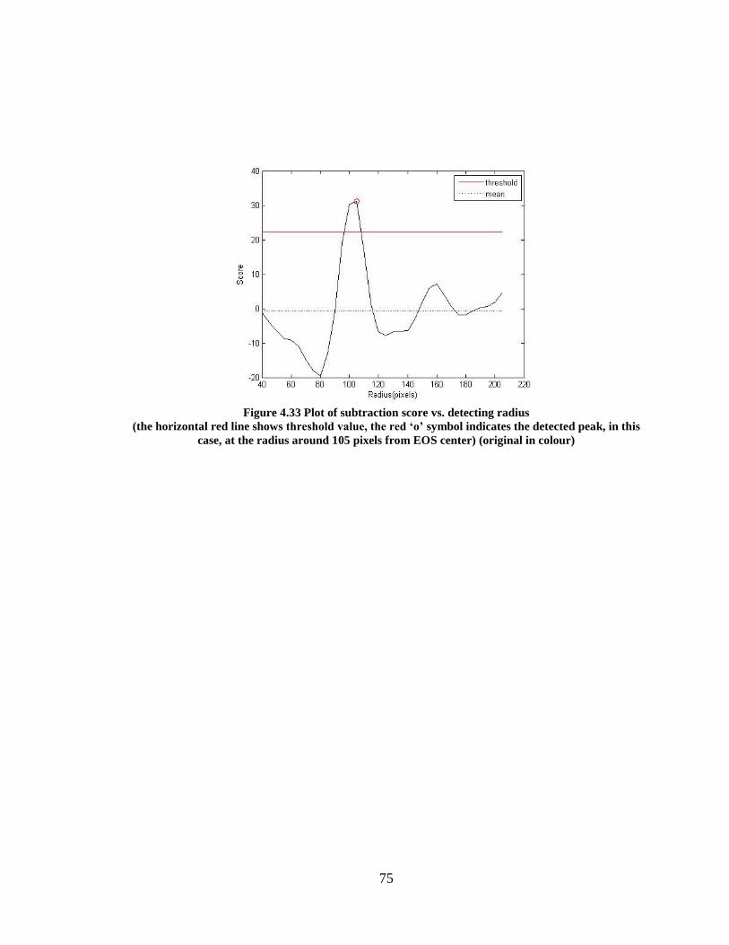
75
Figure 4.33 Plot of subtraction score vs. detecting radius
(the horizontal red line shows threshold value, the red ‘o’ symbol indicates the detected peak, in this
case, at the radius around 105 pixels from EOS center) (original in colour)
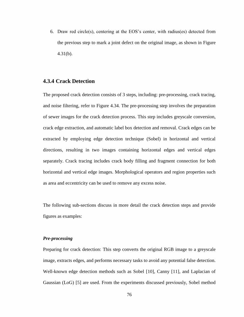
76
6. Draw red circle(s), centering at the EOS’s center, with radius(es) detected from
the previous step to mark a joint defect on the original image, as shown in Figure
4.31(b).
4.3.4 Crack Detection
The proposed crack detection consists of 3 steps, including: pre-processing, crack tracing,
and noise filtering, refer to Figure 4.34. The pre-processing step involves the preparation
of sewer images for the crack detection process. This step includes greyscale conversion,
crack edge extraction, and automatic label box detection and removal. Crack edges can be
extracted by employing edge detection technique (Sobel) in horizontal and vertical
directions, resulting in two images containing horizontal edges and vertical edges
separately. Crack tracing includes crack body filling and fragment connection for both
horizontal and vertical edge images. Morphological operators and region properties such
as area and eccentricity can be used to remove any excess noise.
The following sub-sections discuss in more detail the crack detection steps and provide
figures as examples:
Pre-processing
Preparing for crack detection: This step converts the original RGB image to a greyscale
image, extracts edges, and performs necessary tasks to avoid any potential false detection.
Well-known edge detection methods such as Sobel [10], Canny [11], and Laplacian of
Gaussian (LoG) [5] are used. From the experiments discussed previously, Sobel method
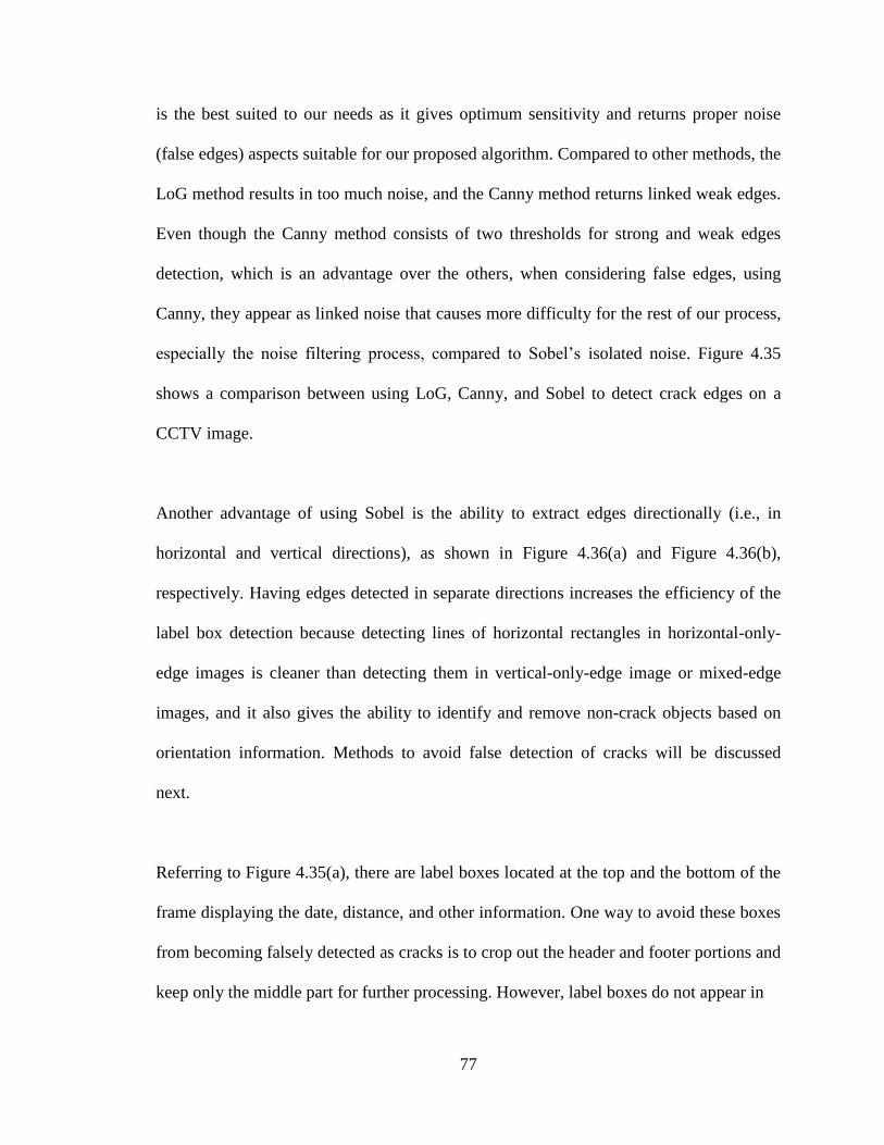
77
is the best suited to our needs as it gives optimum sensitivity and returns proper noise
(false edges) aspects suitable for our proposed algorithm. Compared to other methods, the
LoG method results in too much noise, and the Canny method returns linked weak edges.
Even though the Canny method consists of two thresholds for strong and weak edges
detection, which is an advantage over the others, when considering false edges, using
Canny, they appear as linked noise that causes more difficulty for the rest of our process,
especially the noise filtering process, compared to Sobel’s isolated noise. Figure 4.35
shows a comparison between using LoG, Canny, and Sobel to detect crack edges on a
CCTV image.
Another advantage of using Sobel is the ability to extract edges directionally (i.e., in
horizontal and vertical directions), as shown in Figure 4.36(a) and Figure 4.36(b),
respectively. Having edges detected in separate directions increases the efficiency of the
label box detection because detecting lines of horizontal rectangles in horizontal-only-
edge images is cleaner than detecting them in vertical-only-edge image or mixed-edge
images, and it also gives the ability to identify and remove non-crack objects based on
orientation information. Methods to avoid false detection of cracks will be discussed
next.
Referring to Figure 4.35(a), there are label boxes located at the top and the bottom of the
frame displaying the date, distance, and other information. One way to avoid these boxes
from becoming falsely detected as cracks is to crop out the header and footer portions and
keep only the middle part for further processing. However, label boxes do not appear in
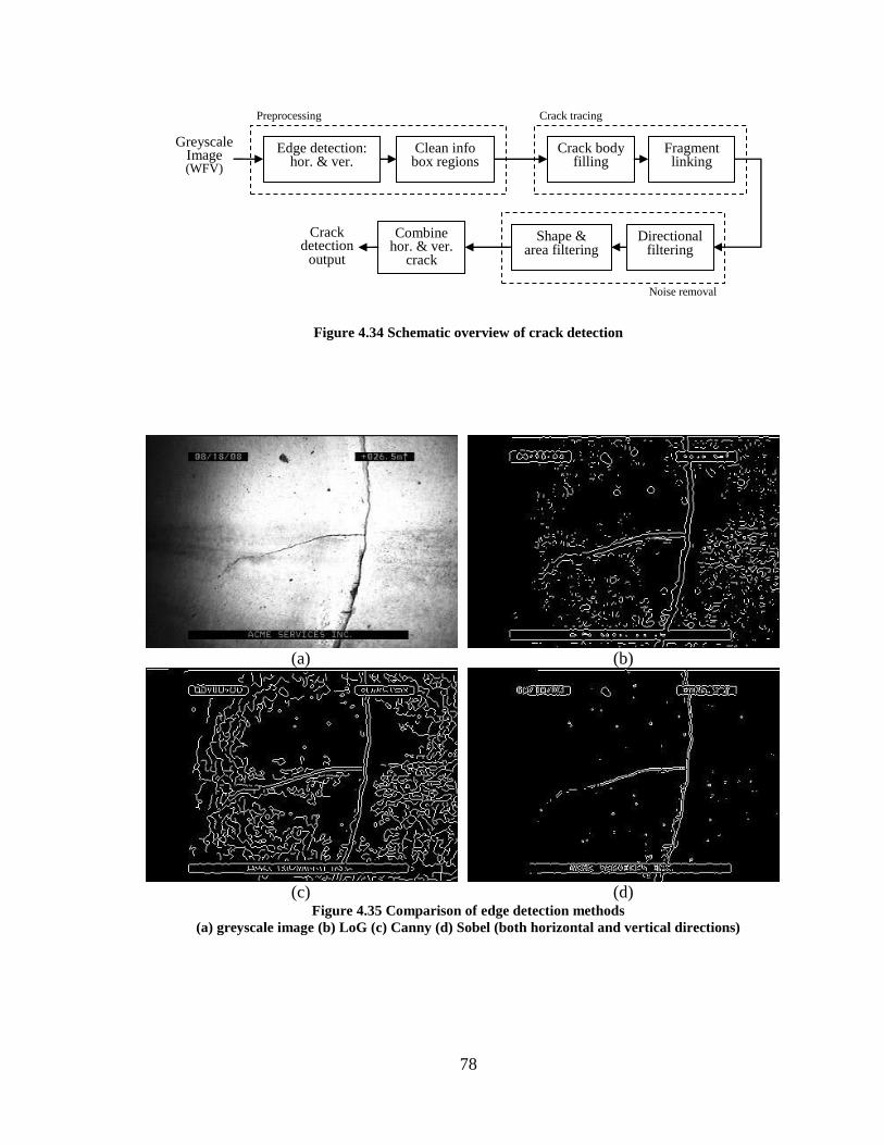
78
Figure 4.34 Schematic overview of crack detection
(a)
(b)
(c)
(d)
Figure 4.35 Comparison of edge detection methods
(a) greyscale image (b) LoG (c) Canny (d) Sobel (both horizontal and vertical directions)
Greyscale Image (WFV)
Edge detection: hor. & ver.
Clean info box regions
Preprocessing
Crack body filling
Fragment linking
Crack tracing
Combine hor. & ver.
crack
Crack detection
output
Directional filtering
Shape & area filtering
Noise removal
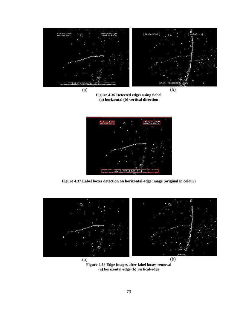
79
(a)
(b)
Figure 4.36 Detected edges using Sobel
(a) horizontal (b) vertical direction
Figure 4.37 Label boxes detection on horizontal-edge image (original in colour)
(a)
(b)
Figure 4.38 Edge images after label boxes removal
(a) horizontal-edge (b) vertical-edge
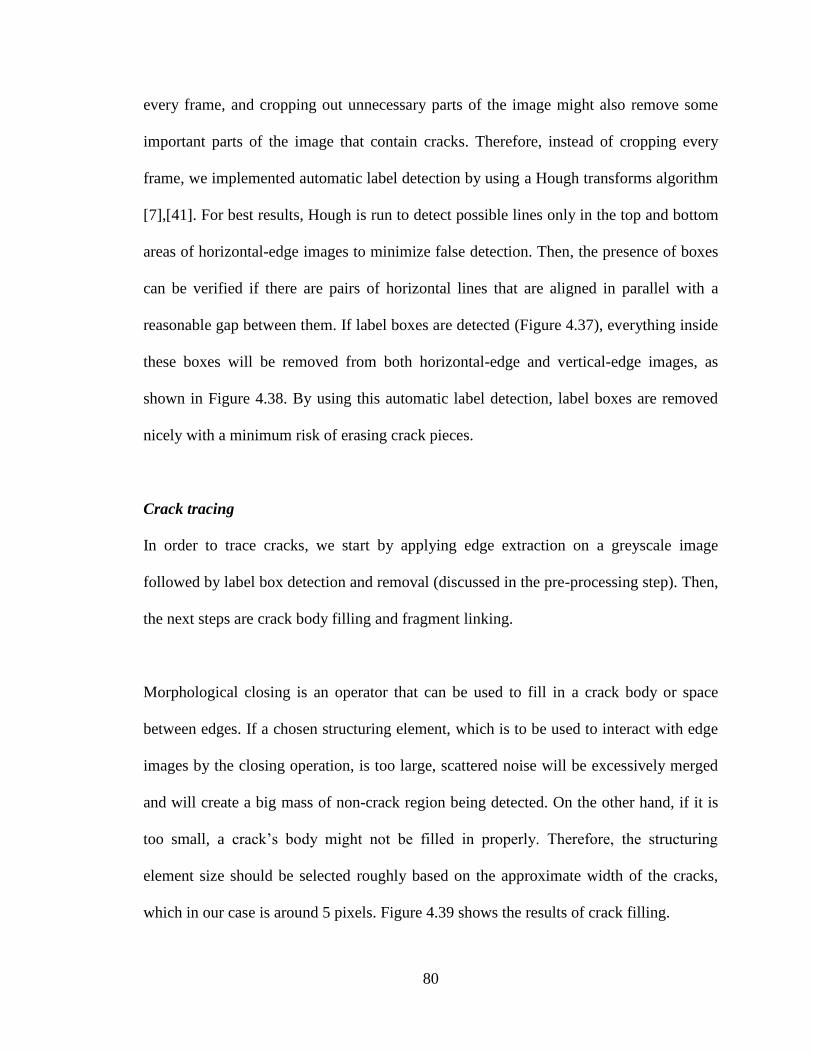
80
every frame, and cropping out unnecessary parts of the image might also remove some
important parts of the image that contain cracks. Therefore, instead of cropping every
frame, we implemented automatic label detection by using a Hough transforms algorithm
[7],[41]. For best results, Hough is run to detect possible lines only in the top and bottom
areas of horizontal-edge images to minimize false detection. Then, the presence of boxes
can be verified if there are pairs of horizontal lines that are aligned in parallel with a
reasonable gap between them. If label boxes are detected (Figure 4.37), everything inside
these boxes will be removed from both horizontal-edge and vertical-edge images, as
shown in Figure 4.38. By using this automatic label detection, label boxes are removed
nicely with a minimum risk of erasing crack pieces.
Crack tracing
In order to trace cracks, we start by applying edge extraction on a greyscale image
followed by label box detection and removal (discussed in the pre-processing step). Then,
the next steps are crack body filling and fragment linking.
Morphological closing is an operator that can be used to fill in a crack body or space
between edges. If a chosen structuring element, which is to be used to interact with edge
images by the closing operation, is too large, scattered noise will be excessively merged
and will create a big mass of non-crack region being detected. On the other hand, if it is
too small, a crack’s body might not be filled in properly. Therefore, the structuring
element size should be selected roughly based on the approximate width of the cracks,
which in our case is around 5 pixels. Figure 4.39 shows the results of crack filling.
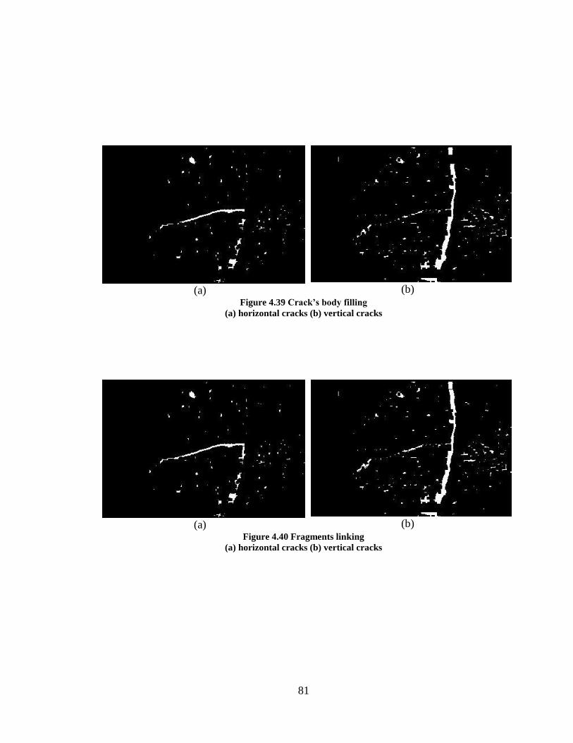
81
(a)
(b)
Figure 4.39 Crack’s body filling
(a) horizontal cracks (b) vertical cracks
(a)
(b)
Figure 4.40 Fragments linking
(a) horizontal cracks (b) vertical cracks

82
Most of the time, there is discontinuity or missing parts of the detected crack’s trace
because of low intensity in that region or due to the camera’s light, for example. Our
crack connection method allows crack fragments to be linked back together; otherwise,
these fragments might be mistakenly removed as noise. Fragments appear as branches
and/or small pieces together and are likely to be an extension or part of the crack. We
categorized crack fragments into 3 types: 1. long branch (length > 100 pixels), 2. short
branch (5 < length 100 pixels), and 3. small piece (length 5 pixels). Any pixel-group
with an area of less than 5 pixels is not accepted as a fragment.
For every pair of one-to-one matching of all fragments in the frame, the closest end-to-
end gap between fragments will be assumed to be a suspicious missing part, and its
distance and angle will be used for valid extension verification. The true extension must
meet all the following criteria:
- both fragments must not belong to type 3 at the same time
- both fragments are likely to lie in the same direction (within reasonable
threshold (e.g., less than 20 degrees difference))
- the gap between fragments at the closest end-to-end points also aligns in the
same direction as the orientation of both fragments
- the closest gap distance (end-to-end) is within a reasonable length
The above criteria allow linking of only fragments that align in the same direction as
another extendable crack fragment. Pieces that are not located close enough to each other
will be ignored. Type 3 or small pieces are not extendable and, hence, should not be able
to link to another type 3. Type 1 and type 2 are able to connect to any types of fragments.
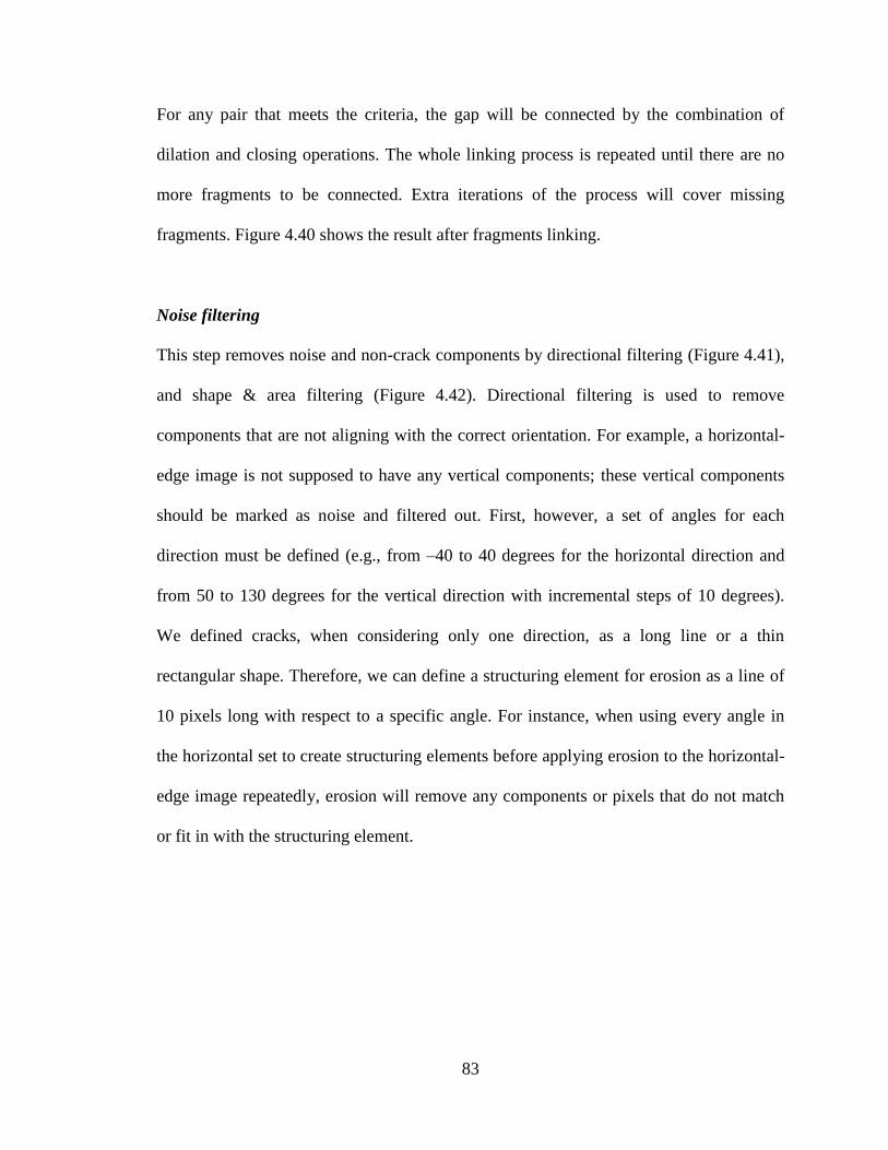
83
For any pair that meets the criteria, the gap will be connected by the combination of
dilation and closing operations. The whole linking process is repeated until there are no
more fragments to be connected. Extra iterations of the process will cover missing
fragments. Figure 4.40 shows the result after fragments linking.
Noise filtering
This step removes noise and non-crack components by directional filtering (Figure 4.41),
and shape & area filtering (Figure 4.42). Directional filtering is used to remove
components that are not aligning with the correct orientation. For example, a horizontal-
edge image is not supposed to have any vertical components; these vertical components
should be marked as noise and filtered out. First, however, a set of angles for each
direction must be defined (e.g., from –40 to 40 degrees for the horizontal direction and
from 50 to 130 degrees for the vertical direction with incremental steps of 10 degrees).
We defined cracks, when considering only one direction, as a long line or a thin
rectangular shape. Therefore, we can define a structuring element for erosion as a line of
10 pixels long with respect to a specific angle. For instance, when using every angle in
the horizontal set to create structuring elements before applying erosion to the horizontal-
edge image repeatedly, erosion will remove any components or pixels that do not match
or fit in with the structuring element.
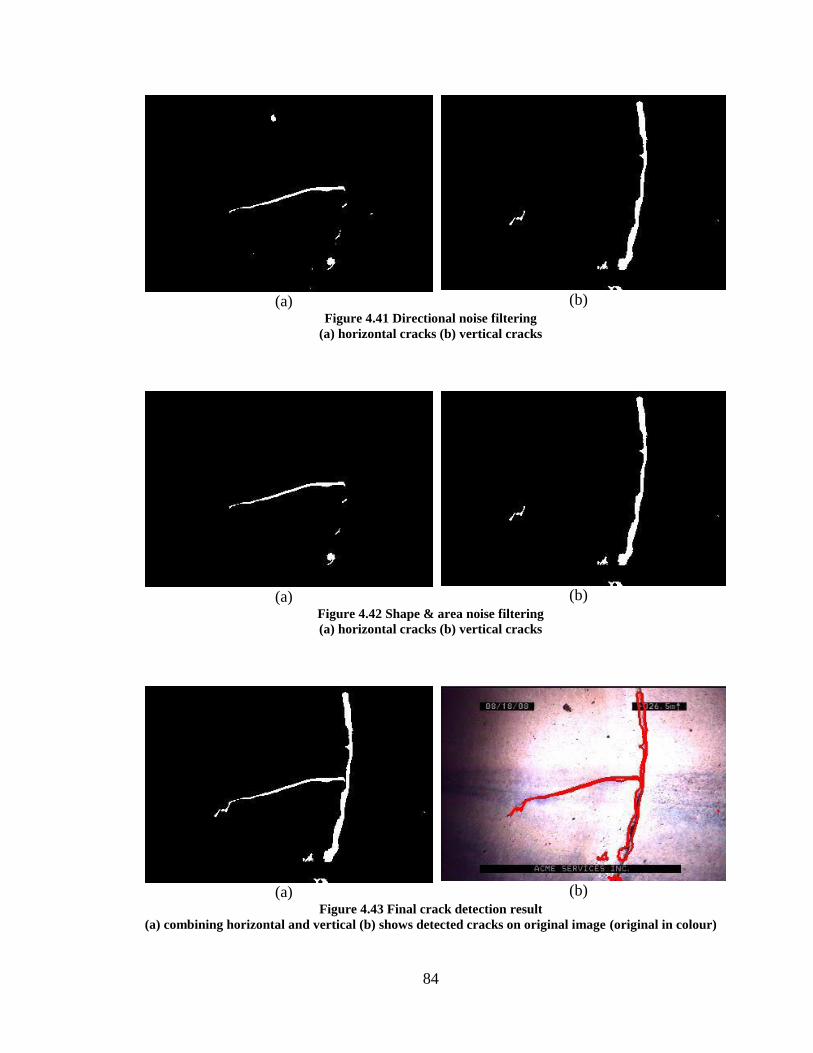
84
(a)
(b)
Figure 4.41 Directional noise filtering
(a) horizontal cracks (b) vertical cracks
(a)
(b)
Figure 4.42 Shape & area noise filtering
(a) horizontal cracks (b) vertical cracks
(a)
(b)
Figure 4.43 Final crack detection result
(a) combining horizontal and vertical (b) shows detected cracks on original image (original in colour)

85
In fact, either erosion or opening can be used as a noise-filtering tool. However, we
decided to use erosion with the purpose of also removing some mess or excess regions
caused by unwanted merging of cracks and nearby noise from the filling and connecting
process. Hence, another advantage of this step is that cracks also get smoothed.
In the directional filtering, it is quite certain that most non-crack components will be
removed. However, several non-crack components might still exist if their area is large
enough. The remaining non-crack area mostly appears as shapeless groups of pixels,
whereas crack area is more likely to be a long, linear segment. Therefore, shape & area
filtering is needed to filter out these remaining non-crack components by using region
properties including eccentricity and area. The eccentricity can be used to determine the
shape of regions. It is defined as “the ratio of the distance between the foci of the ellipse
and its major axis length” [55]. The eccentricity has a value ranging from 0 to 1. A value
closer to zero indicates a shape more like a circle, and a value closer to one indicates a
shape more like a line. From our experiment, an eccentricity value of around 0.9 is the
bottom limit of accepting a shape as a crack. Therefore, any fragments whose eccentricity
is less than 0.9 will be removed.
The next step is to filter the remaining components by area. The area property of any
region means the total number of pixels within that region. We chose a reasonable value
based on experimentation to be a criterion for the smallest acceptable area. This value
should be big enough to get rid of small noise but not too big so as to preserve true

86
cracks. Figure 4.43 shows the final crack detection result after combining horizontal and
vertical cracks.
CCTV images do not present the actual size of defects due to zooming ability and
unknown distance from camera to defect. Therefore, defects size measurement and
severity assessment are not feasible.
4.3.5 Defect Confidence Level
The defect detection process is not always 100% accurate; therefore, a confidence level
was introduced to provide information of how likely a detected defect will be a true
positive result. The confidence level is a percentage of the number of frames in which the
defect is detected over the total number of frames in that ROI group. It is computed for
each type of detected defects. If a detection result has a low confidence level, then there
is a low probability of that defect actually appearing in the ROI. On the other hand, there
is a high chance of true positive detection if the confidence level is high.
87
Chapter 5
RESULTS AND DISCUSSION
This chapter evaluates the robustness and performance of the proposed algorithms and
describes any limitations that may cause errors. The chapter describes experimental
results on each of the aforementioned processes. Figures showing examples of success
and/or failure are illustrated. Results in this chapter were generated using actual CCTV
video files provided by the City of Regina.
5.1 Regions of Interest Extraction
This section describes the efficiency of the ROIs Extraction process in terms of workload
reduction and accuracy of position approximation.
5.1.1 Workload Reduced by Regions of Interest Extraction
Table 5.1 shows workload reduction by applying ROIs Extraction to four CCTV videos:
“V5”, “V8”, “V03”, and “Video_1”. Workload reduction rate is a ratio of the number of
fames outside ROI groups to the total number of frames of the whole video length. A
greater workload reduction rate (closer to 1.0) means a lower number of frames and less
processing time will be required for frame classification, segmentation, and defect
detection.
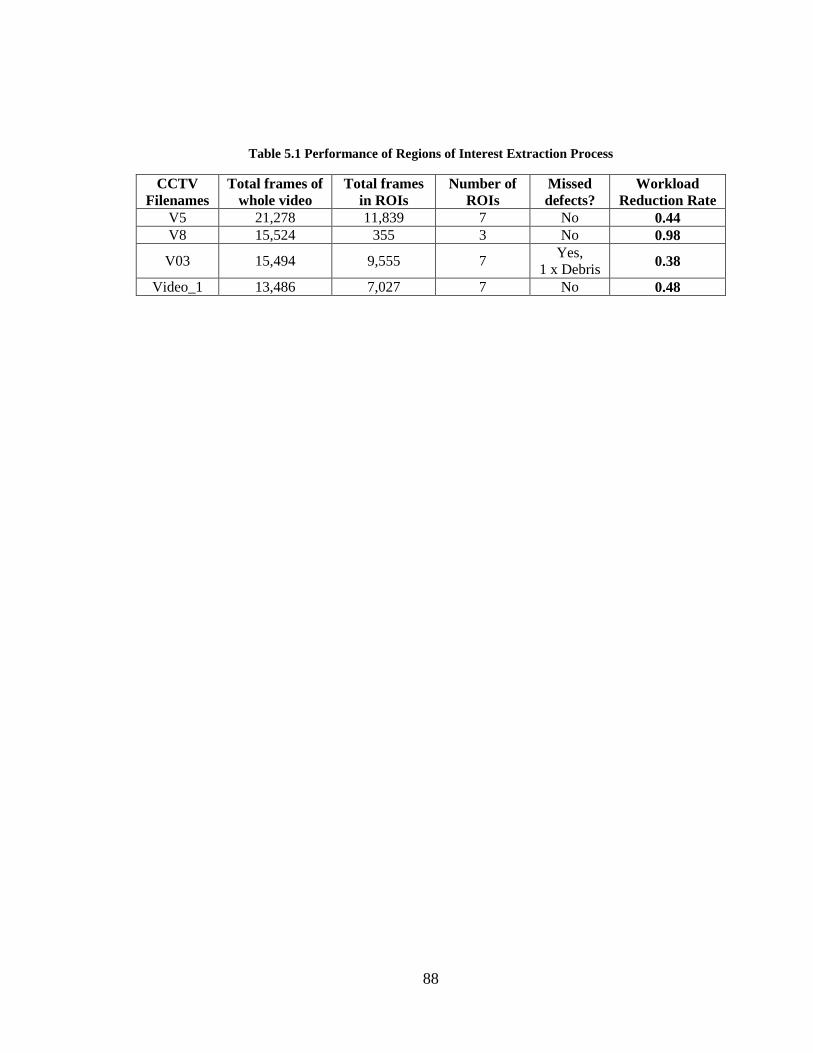
88
Table 5.1 Performance of Regions of Interest Extraction Process
CCTV
Filenames
Total frames of
whole video
Total frames
in ROIs
Number of
ROIs
Missed
defects?
Workload
Reduction Rate
V5 21,278 11,839 7 No 0.44
V8 15,524 355 3 No 0.98
V03 15,494 9,555 7 Yes,
1 x Debris 0.38
Video_1 13,486 7,027 7 No 0.48
89
The table shows that workloads were reduced by 38% up to 98% of total work that would
be required without ROIs Extraction. Defects were all captured in ROI groups, except
one set of debris that was missing from one of the ROI groups (video “V03”). This
occurred only because the camera operator passed by this location continuously without
slowing down or stopping. Frames outside ROI groups will be discarded and any left out
defects will be undetectable.
In summary, the ROIs Extraction process helped reduce a huge amount of work from the
videos’ total length. However, some defects might be undetectable in situations when
camera operators do not stop or slow down when approaching or passing defects.
5.1.2 Position Approximation
A test was set up to verify position approximation performance by comparing positions
estimated by the proposed optical flow-based method with positions estimated by a
simple video timeline progressing-based method. Equation (5-1) shows the calculation of
video timeline method.
N
nMHDpositionn
(5-1)
where: n = current considering frame, N = total frame number
MHD = actual distance between manholes or actual survey distance in video (meters)
90
The actual positions (ground truth) were recorded every 100 frames manually from
CCTV video frames (usually shown on top-right or bottom-right corner of frames).
Figure 5.1 shows very nice plots and very close to ground truth of our optical flow-based
method. Table 5.2 shows that average absolute-distance error of position approximation
of the four videos ranges from around 3 m. to 12 m. by video timeline method and around
1 m. to 3 m. by our optical flow method.
The results show that our position approximation with the optical flow technique
improved up to 10 m. closer to actual sewer position when compared to basic video
timeline estimation. However, videos with massive tilt or rotation have a higher chance of
error than smoother videos.
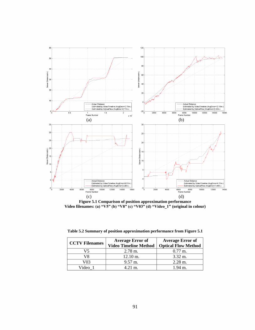
91
(a)
(b)
(c)
(d)
Figure 5.1 Comparison of position approximation performance
Video filenames: (a) “V5” (b) “V8” (c) “V03” (d) “Video_1” (original in colour)
Table 5.2 Summary of position approximation performance from Figure 5.1
CCTV Filenames Average Error of
Video Timeline Method
Average Error of
Optical Flow Method
V5 2.78 m. 0.77 m.
V8 12.10 m. 3.32 m.
V03 9.57 m. 2.28 m.
Video_1 4.21 m. 1.94 m.
92
5.2 Sewer Frame Classification and Segmentation
5.2.1 Frame Classification
The objectives of frame classification are to reduce false defect detection and to reduce
processing time by skipping some detection processing for inapplicable frames. Frame
classification uses Haar wavelet feature extraction and SVM multiclass classification
with a Radial Basis Function (RBF) kernel.
Tables 5.3 to 5.6 show the accuracy of classifying ROI frames into FFV, TV, WFV, and
INFO frame categories in videos “V5”, “V8”, “V03”, and “Video_1”. All ROI frames of
Video “V5” are FFV frames; only 0.35% of them are misclassified. Table 5.5 shows 85
frames out of 87 are actually WFV frames of video “V03” misclassified into FFV
category. Our examination found that these 85 frames consist of dark areas at the bottom
of frames and are close to the water composition in FFV frames. Also, FFV frames in
“Video_1” are quite ambiguous due to dark bands on the side walls and no water flow in
some frames; this resulted in around 25% of FFV frames being misclassified into the TV
frame category. However, an overall performance of 80% accuracy for “Video_1” is still
regarded as a good performance.
In summary, frame classification yields from 80% up to 99% accuracy. More training
examples and proper parameters tuning and feature selection during the SVM learning
process would reduce the misclassification rate.

93
Table 5.3 Confusion matrix of frame classification – Video “V5”
SVM
RBF
Predicted Total
FFV TV WFV INFO
Act
ual
FFV 11,797 0 0 42 11,839
TV 0 0 0 0 0
WFV 0 0 0 0 0
INFO 0 0 0 0 0
Total 11,797 0 0 42 11,839
Accuracy = 99.65%
Table 5.4 Confusion matrix of frame classification – Video “V8”
SVM
RBF
Predicted Total
FFV TV WFV INFO
Act
ual
FFV 0 0 0 0 0
TV 0 0 0 0 0
WFV 35 0 230 0 265
INFO 0 0 0 90 90
Total 35 0 230 90 355
Accuracy = 90.14%
Table 5.5 Confusion matrix of frame classification – Video “V03”
SVM
RBF
Predicted Total
FFV TV WFV INFO
Act
ual
FFV 9,147 2 0 0 9,149
TV 0 130 0 0 130
WFV 85 0 2 0 87
INFO 2 0 0 187 189
Total 9,234 132 2 187 9,555
Accuracy = 99.07%
Table 5.6 Confusion matrix of frame classification – Video “Video_1”
SVM
RBF
Predicted Total
FFV TV WFV INFO
Act
ual
FFV 2,130 846 247 232 3,455
TV 3 154 0 0 157
WFV 4 61 3,095 0 3,160
INFO 0 0 0 255 255
Total 2,137 1,061 3,342 487 7,027
Accuracy = 80.18%
94
5.2.2 EOS Location Search and Verification
Figure 5.2 illustrates sewer EOS location search results for both dark and bright EOS
images. A cross-section of vertical and horizontal lines indicates the detected EOS center
position. Figure 5.2(a), (b), and (c) shows very good and acceptable results. However,
Figure 5.2(d) shows a misplaced location due to failure from the EOS type auto-
determination algorithm. The location searching used incorrect steps for dark instead of
the proper steps for a bright EOS. However, it eventually was rejected as a fault location
by the EOS verification process.
From the experiment on 100 FFV images, our EOS location search process together with
EOS type auto-determination and EOS location verification gave an excellent
performance of 82% accuracy. EOS verification can also be used to avoid
misclassification of FFV frames and WFV frames by checking for the presence of sewer
EOS.
Note: If the user defines the EOS type (“dark” or “bright”), the EOS type auto-
determination feature will be turned off, which could reduce chances of error in case
when the type is already known. Enabling the EOS type auto-determination is, however,
preferred when dealing with a video set that includes both dark and bright EOS areas12
.
12
For example, some videos might be captured by different camera robot models that result in different
appearances of sewer scenes including but not limited to the colour of the EOS.
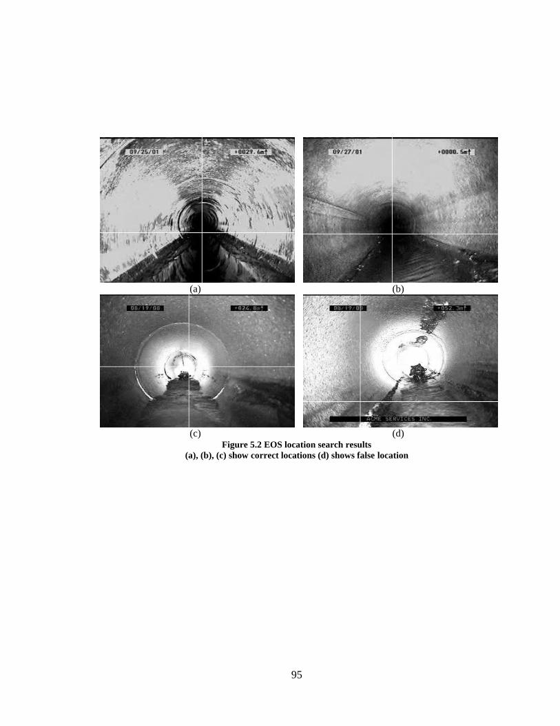
95
(a)
(b)
(c)
(d)
Figure 5.2 EOS location search results
(a), (b), (c) show correct locations (d) shows false location
96
5.2.3 Water Flow Line Estimation and Verification
The flow line estimation algorithm works by detecting pixel intensity jump at four scan
lines. Applicable frames must have water at the bottom of the frame with a dark colour
and walls with brighter colour. Use of four (or more) scan lines, instead of just one,
reduces the chance of error of incorrect points being selected caused by some bright
pixels or debris in the water. However, if the flow line estimation, in some cases, returns
incorrect detection, it will eventually be rejected by the verification process.
The water flow line estimation and verification performs well with 75% accuracy of the
testing performed on 100 FFV images (refer to Figure 5.3 for an example of the results).
Further adjustment of the alignment of scan lines would improve flow line estimation
accuracy. However, our flow line estimation algorithm will definitely fail when dealing
with sewer CCTV images that appear to have no water or no dark triangle shape on the
frame’s lower edge.
.
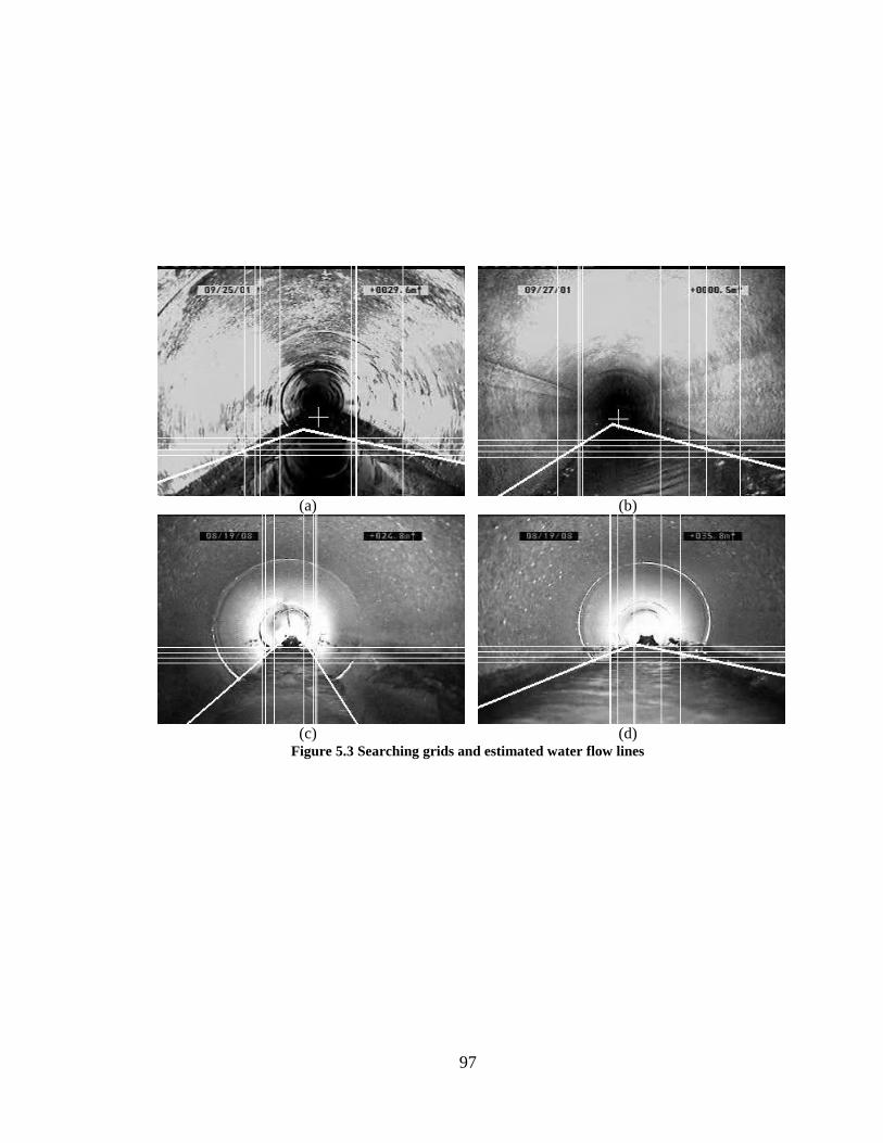
97
(a)
(b)
(c)
(d)
Figure 5.3 Searching grids and estimated water flow lines
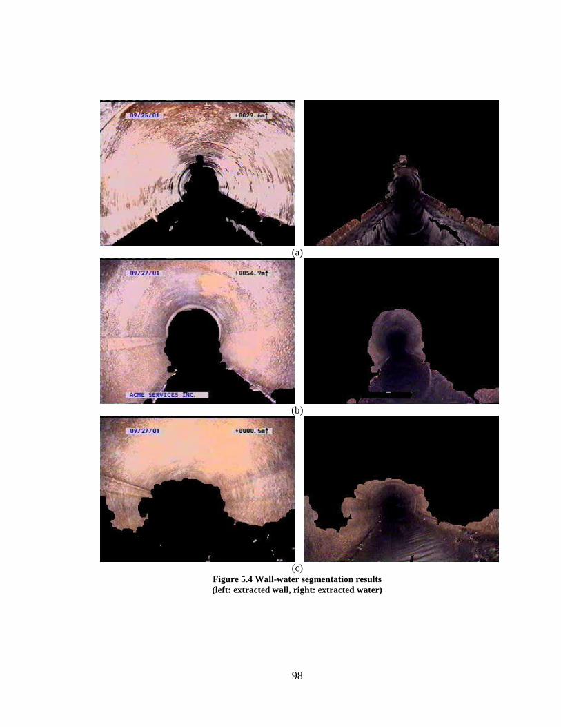
98
(a)
(b)
(c)
Figure 5.4 Wall-water segmentation results
(left: extracted wall, right: extracted water)
99
5.2.4 Wall-Water Segmentation
Wall-water segmentation returned excellent results as seen in the example shown in
Figure 5.4. Even though the water segment of Figure 5.4(c) extended into the region that
is supposed to be sewer’s wall, this will not affect the debris detection process because
debris detection only needs to pick up bright objects inside the water flow line region
after segmentation; hence, any region beyond the flow line is negligible.
Note that the wall-water segmentation will be successful when sewer frames are
composed of water flow (i.e., a dark triangle shape sitting on the lower portion of
frames).
5.2.5 Information Label Box Detection
The information label box detection plays a significant role in the debris detection and
crack detection processes by avoiding the interference of these boxes, which are usually
of unknown size and position, with detection of actual defects. Our Hough transform-
based box detection works properly with only a small chance of misdetection when part
of or a whole box is surrounded by similar background intensity such as a white box on a
very bright background or black box on a very dark background. Referring to Figure
5.5(d), only one label box on the top-right of the frame was undetected while all other
label boxes were correctly recognised. Figure 5.5(a), (b), and (c) show perfect label box
detection output.
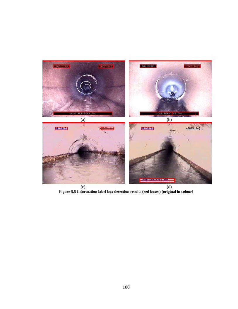
100
(a)
(b)
(c)
(d)
Figure 5.5 Information label box detection results (red boxes) (original in colour)
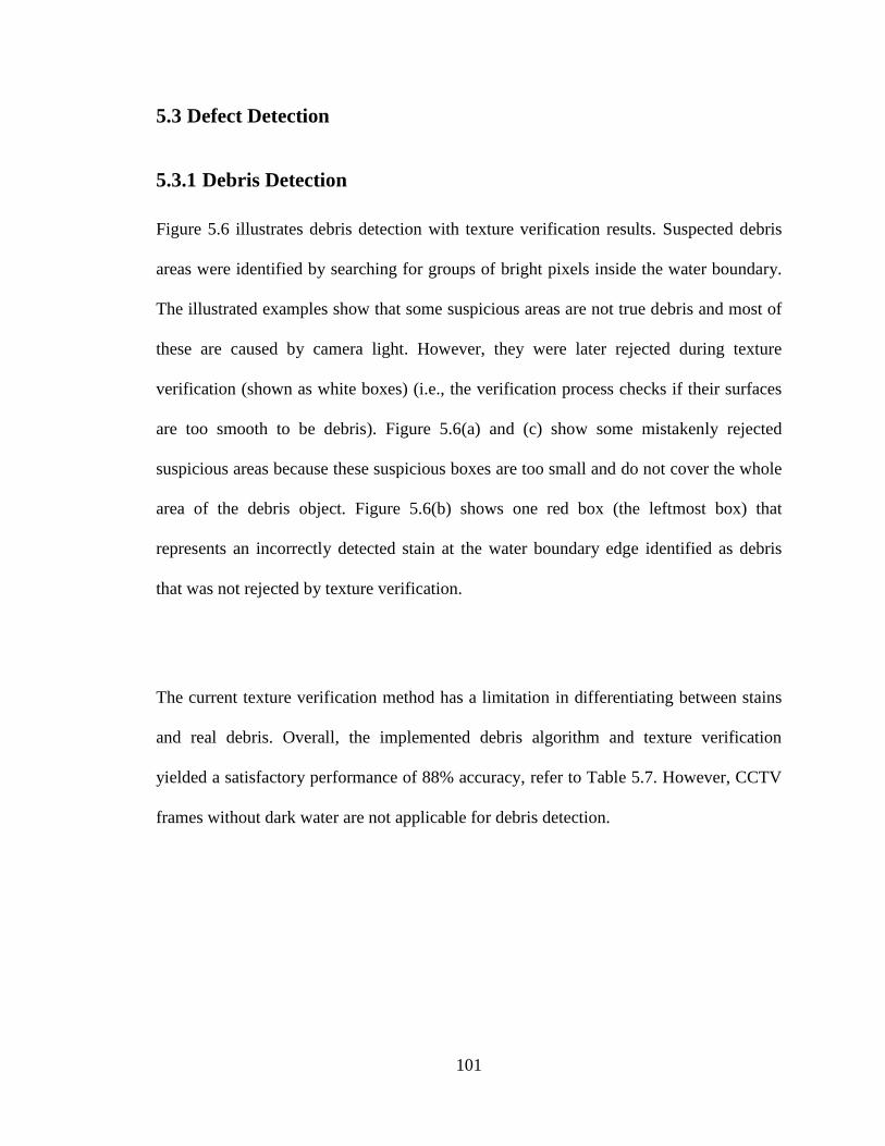
101
5.3 Defect Detection
5.3.1 Debris Detection
Figure 5.6 illustrates debris detection with texture verification results. Suspected debris
areas were identified by searching for groups of bright pixels inside the water boundary.
The illustrated examples show that some suspicious areas are not true debris and most of
these are caused by camera light. However, they were later rejected during texture
verification (shown as white boxes) (i.e., the verification process checks if their surfaces
are too smooth to be debris). Figure 5.6(a) and (c) show some mistakenly rejected
suspicious areas because these suspicious boxes are too small and do not cover the whole
area of the debris object. Figure 5.6(b) shows one red box (the leftmost box) that
represents an incorrectly detected stain at the water boundary edge identified as debris
that was not rejected by texture verification.
The current texture verification method has a limitation in differentiating between stains
and real debris. Overall, the implemented debris algorithm and texture verification
yielded a satisfactory performance of 88% accuracy, refer to Table 5.7. However, CCTV
frames without dark water are not applicable for debris detection.
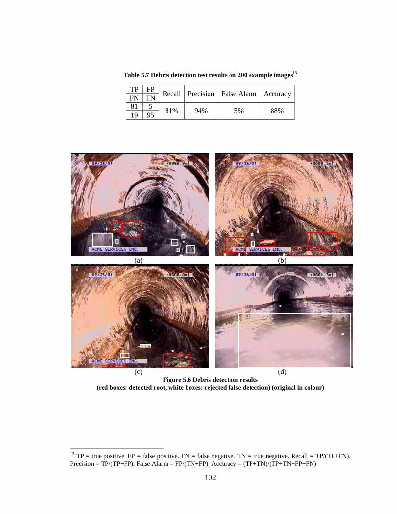
102
Table 5.7 Debris detection test results on 200 example images13
TP FP Recall Precision False Alarm Accuracy
FN TN
81 5 81% 94% 5% 88%
19 95
(a)
(b)
(c)
(d)
Figure 5.6 Debris detection results
(red boxes: detected root, white boxes: rejected false detection) (original in colour)
13
TP = true positive. FP = false positive. FN = false negative. TN = true negative. Recall = TP/(TP+FN).
Precision = TP/(TP+FP). False Alarm = FP/(TN+FP). Accuracy = (TP+TN)/(TP+TN+FP+FN)
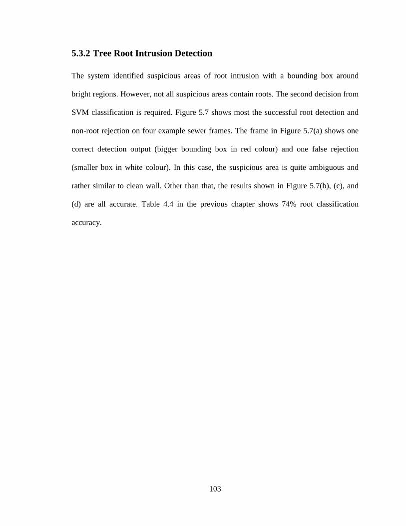
103
5.3.2 Tree Root Intrusion Detection
The system identified suspicious areas of root intrusion with a bounding box around
bright regions. However, not all suspicious areas contain roots. The second decision from
SVM classification is required. Figure 5.7 shows most the successful root detection and
non-root rejection on four example sewer frames. The frame in Figure 5.7(a) shows one
correct detection output (bigger bounding box in red colour) and one false rejection
(smaller box in white colour). In this case, the suspicious area is quite ambiguous and
rather similar to clean wall. Other than that, the results shown in Figure 5.7(b), (c), and
(d) are all accurate. Table 4.4 in the previous chapter shows 74% root classification
accuracy.
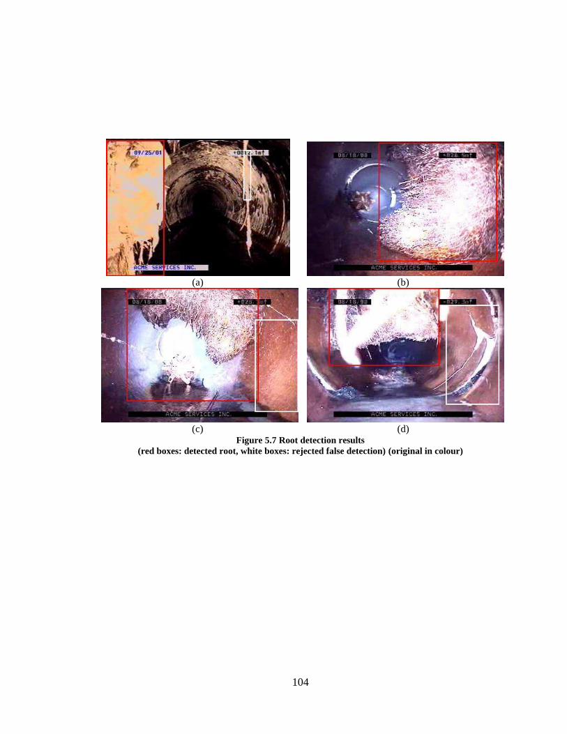
104
(a)
(b)
(c)
(d)
Figure 5.7 Root detection results
(red boxes: detected root, white boxes: rejected false detection) (original in colour)
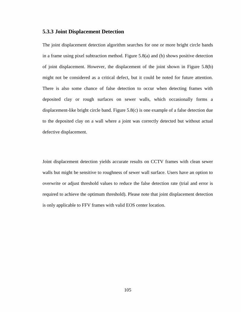
105
5.3.3 Joint Displacement Detection
The joint displacement detection algorithm searches for one or more bright circle bands
in a frame using pixel subtraction method. Figure 5.8(a) and (b) shows positive detection
of joint displacement. However, the displacement of the joint shown in Figure 5.8(b)
might not be considered as a critical defect, but it could be noted for future attention.
There is also some chance of false detection to occur when detecting frames with
deposited clay or rough surfaces on sewer walls, which occasionally forms a
displacement-like bright circle band. Figure 5.8(c) is one example of a false detection due
to the deposited clay on a wall where a joint was correctly detected but without actual
defective displacement.
Joint displacement detection yields accurate results on CCTV frames with clean sewer
walls but might be sensitive to roughness of sewer wall surface. Users have an option to
overwrite or adjust threshold values to reduce the false detection rate (trial and error is
required to achieve the optimum threshold). Please note that joint displacement detection
is only applicable to FFV frames with valid EOS center location.
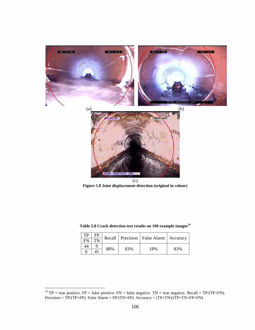
106
(a)
(b)
(c)
Figure 5.8 Joint displacement detection (original in colour)
Table 5.8 Crack detection test results on 100 example images14
TP FP Recall Precision False Alarm Accuracy
FN TN
44 9 88% 83% 18% 83%
6 41
14
TP = true positive. FP = false positive. FN = false negative. TN = true negative. Recall = TP/(TP+FN).
Precision = TP/(TP+FP). False Alarm = FP/(TN+FP). Accuracy = (TP+TN)/(TP+TN+FP+FN)

107
5.3.4 Crack Detection
Figure 5.9 illustrates the results of crack detection on WFV frames. The software marked
cracks correctly and effectively discarded most noise and ignored information label
boxes. The crack detection algorithm also worked well even on blurry images as shown
in Figure 5.9(c). However, some discontinuity of crack detection occurred where there
was light reflection causing some small fragments to be harder to recognise. It, thus,
could be improved, but this is an offset to not getting too much noise and false detection,
which is considered to be more important to avoid. Table 5.8 shows 83% accuracy of the
experiment on 100 images (50 cracks and 50 clean images). There is a restriction in terms
of measuring the actual size of detected cracks due to unknown image scaling from the
zoom-able camera, and unknown distance to objects.
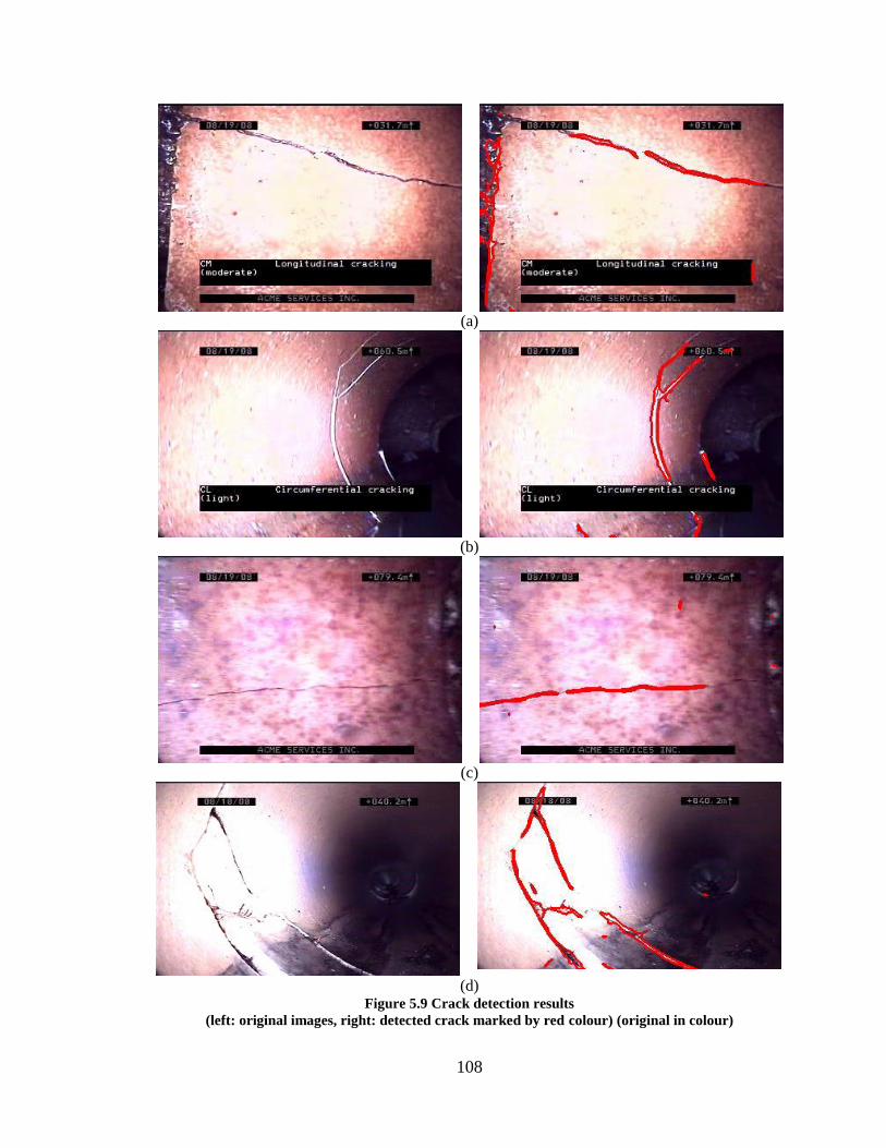
108
(a)
(b)
(c)
(d) Figure 5.9 Crack detection results
(left: original images, right: detected crack marked by red colour) (original in colour)
109
5.4 Overall System Performance
This section shows overall performance of the Automated CCTV Sewer Inspection in
comparison to inspection reports that came with video files provided by the City of
Regina. An example of operator’s inspection report can be found in Appendix C. The
tests used the default values of all parameters and thresholds, which can be found in
Chapter 4. Average time consumption was around 2-3 hours per one video file,
depending on the number of ROI frames. However, because currently all defect detection
functions were implemented in MATLAB, time consumption could be reduced by
optimizing and re-coding all MATLAB functions in C++ when time permits.
In one ROI group, there could be more than one defect, and these defects are usually
present almost the entire length of the ROI group. This means that it is not necessary that
these defects must be detected in all frames or with 100% accuracy but rather should be
detected in a majority of the frames within a group. For example, if one ROI group really
consists of a root, the number of frames that marked root detected should be more than
50% of the total frames of the group (called detection confidence). On the other hand, if a
group does not contain any root, the number of frames that are marked as having a root
detected should be very small.
Tables 5.9 to 5.11 present assessment reports completed by human operators, including
sewer distance position (m.) and defects type and description versus the detection output
of our system, including ROI approximated position, severity ranking, type of detected
110
defects, and detection confidence rate. The tables also include judgements of whether the
results are true or false detections with corresponding figures and/or explanations as
applicable. The ground truth of judgement was based on physical defects displayed in
videos.
The comparison tables show that most defects reported by operators are also reported by
our inspection system with high confidence rates and most false detections came with
quite low confidence. Few defects failed to be detected, outside of those that are currently
not supported by our system due to the limitations that were previously discussed and
might be able to be improved in future work. Our system actually outperformed human
operators at some places where the human operators failed to recognise defects, such as
debris at the beginning of video “V5”. Overall, the inspection system yielded very highly
satisfactory performance.
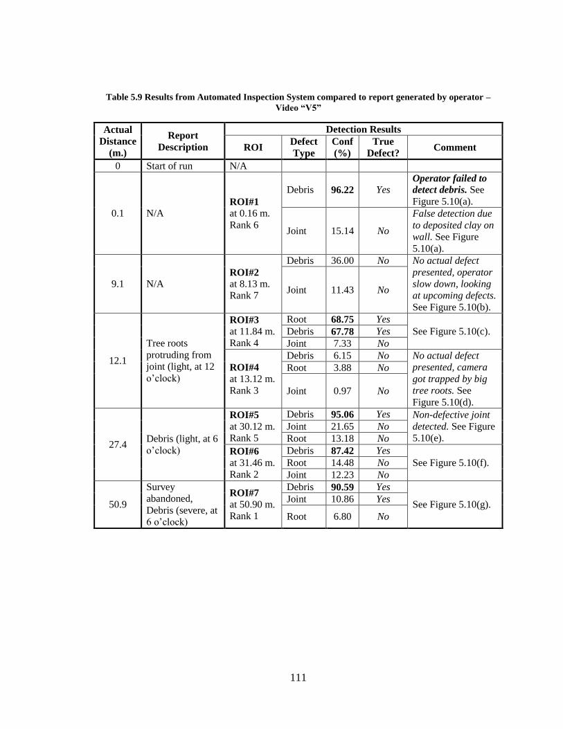
111
Table 5.9 Results from Automated Inspection System compared to report generated by operator –
Video “V5”
Actual
Distance
(m.)
Report
Description
Detection Results
ROI Defect
Type
Conf
(%)
True
Defect? Comment
0 Start of run N/A
0.1 N/A ROI#1
at 0.16 m.
Rank 6
Debris 96.22 Yes Operator failed to
detect debris. See
Figure 5.10(a).
Joint 15.14 No
False detection due
to deposited clay on
wall. See Figure
5.10(a).
9.1 N/A ROI#2
at 8.13 m.
Rank 7
Debris 36.00 No No actual defect
presented, operator
slow down, looking
at upcoming defects.
See Figure 5.10(b).
Joint 11.43 No
12.1
Tree roots
protruding from
joint (light, at 12
o’clock)
ROI#3
at 11.84 m.
Rank 4
Root 68.75 Yes
See Figure 5.10(c). Debris 67.78 Yes
Joint 7.33 No
ROI#4
at 13.12 m.
Rank 3
Debris 6.15 No No actual defect
presented, camera
got trapped by big
tree roots. See
Figure 5.10(d).
Root 3.88 No
Joint 0.97 No
27.4 Debris (light, at 6
o’clock)
ROI#5
at 30.12 m.
Rank 5
Debris 95.06 Yes Non-defective joint
detected. See Figure
5.10(e).
Joint 21.65 No
Root 13.18 No
ROI#6
at 31.46 m.
Rank 2
Debris 87.42 Yes
See Figure 5.10(f). Root 14.48 No
Joint 12.23 No
50.9
Survey
abandoned,
Debris (severe, at
6 o’clock)
ROI#7
at 50.90 m.
Rank 1
Debris 90.59 Yes
See Figure 5.10(g). Joint 10.86 Yes
Root 6.80 No
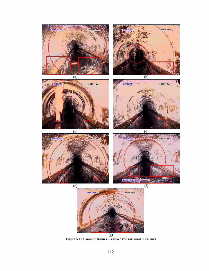
112
(a)
(b)
(c)
(d)
(e)
(f)
(g)
Figure 5.10 Example frames – Video “V5” (original in colour)
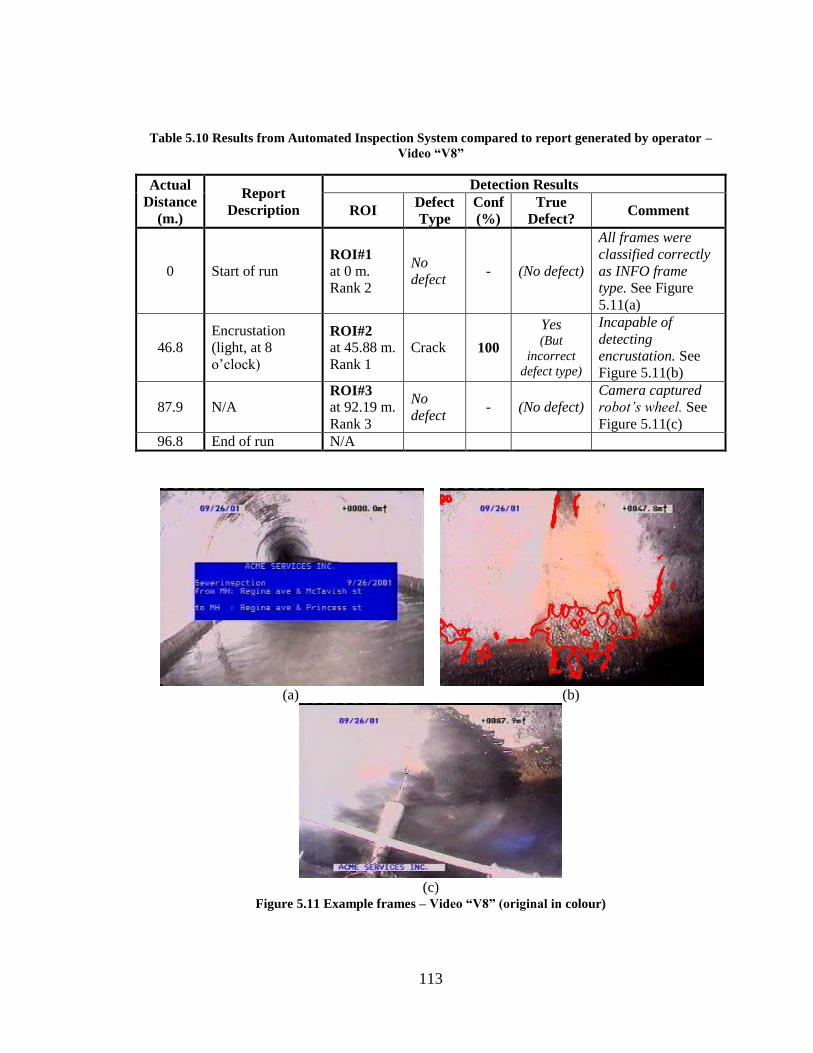
113
Table 5.10 Results from Automated Inspection System compared to report generated by operator –
Video “V8”
Actual
Distance
(m.)
Report
Description
Detection Results
ROI Defect
Type
Conf
(%)
True
Defect? Comment
0 Start of run ROI#1
at 0 m.
Rank 2
No
defect - (No defect)
All frames were
classified correctly
as INFO frame
type. See Figure
5.11(a)
46.8
Encrustation
(light, at 8
o’clock)
ROI#2
at 45.88 m.
Rank 1
Crack 100
Yes (But
incorrect
defect type)
Incapable of
detecting
encrustation. See
Figure 5.11(b)
87.9 N/A ROI#3
at 92.19 m.
Rank 3
No
defect - (No defect)
Camera captured
robot’s wheel. See
Figure 5.11(c)
96.8 End of run N/A
(a)
(b)
(c)
Figure 5.11 Example frames – Video “V8” (original in colour)
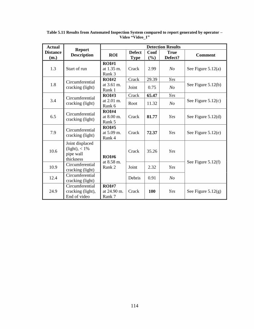
114
Table 5.11 Results from Automated Inspection System compared to report generated by operator –
Video “Video_1”
Actual
Distance
(m.)
Report
Description
Detection Results
ROI Defect
Type
Conf
(%)
True
Defect? Comment
1.3 Start of run ROI#1 at 1.35 m.
Rank 3
Crack 2.99 No See Figure 5.12(a)
1.8 Circumferential
cracking (light)
ROI#2
at 3.61 m.
Rank 1
Crack 29.39 Yes
See Figure 5.12(b) Joint 0.75 No
3.4 Circumferential
cracking (light)
ROI#3
at 2.01 m.
Rank 6
Crack 65.47 Yes
See Figure 5.12(c) Root 11.32 No
6.5 Circumferential
cracking (light)
ROI#4
at 8.00 m.
Rank 5
Crack 81.77 Yes See Figure 5.12(d)
7.9 Circumferential
cracking (light)
ROI#5
at 5.09 m.
Rank 4
Crack 72.37 Yes See Figure 5.12(e)
10.6
Joint displaced
(light), < 1%
pipe wall
thickness ROI#6
at 8.58 m.
Rank 2
Crack 35.26 Yes
See Figure 5.12(f)
10.9 Circumferential
cracking (light) Joint 2.32 Yes
12.4 Circumferential
cracking (light) Debris 0.91 No
24.9
Circumferential
cracking (light),
End of video
ROI#7
at 24.90 m.
Rank 7
Crack 100 Yes See Figure 5.12(g)
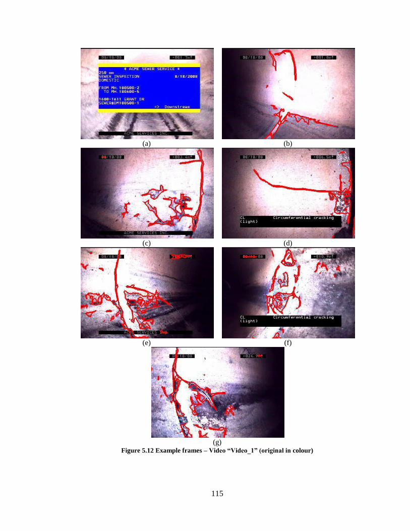
115
(a)
(b)
(c)
(d)
(e)
(f)
(g)
Figure 5.12 Example frames – Video “Video_1” (original in colour)

116
Table 5.12 summarises the performance of the Automated CCTV Sewer Inspection tested
on the example videos, whose detection results were presented in Tables 5.9 to 5.11. The
table includes the confusion matrices and the performance measurement, when applying a
cut-off point of 50% confidence (i.e., threshold for accepting or rejecting detected
defects). If a defect is detected with a confidence rate lower than the cut-off point, the
detection will be rejected. The accepted detection confidence was also highlighted in
bold in Tables 5.9 to 5.11.
Table 5.12 shows 0.81 average recall rate of the example videos. However, the individual
recall rate of videos “Video_1” (0.57) might not be ideally sufficient. The low recall rate
suggests that the system should be improved to reduce the number of missed detections
of defects. Next, the precision rate and true negative rate in Table 5.12 are extremely
high, which means that the system detected (and rejected) defects correctly with a very
low number of false alarms. Finally, the table also indicates that the proposed automated
inspection system yields high average accuracy of around 0.89.
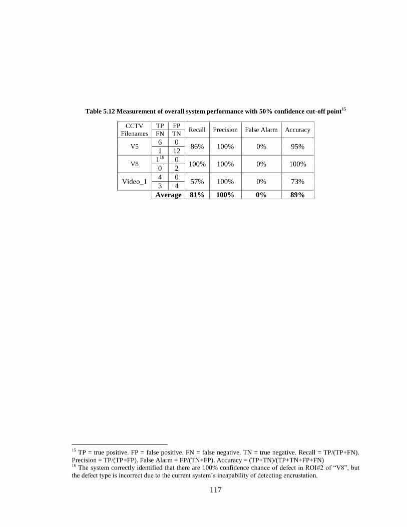
117
Table 5.12 Measurement of overall system performance with 50% confidence cut-off point15
CCTV
Filenames
TP FP Recall Precision False Alarm Accuracy
FN TN
V5 6 0
86% 100% 0% 95% 1 12
V8 1
16 0
100% 100% 0% 100% 0 2
Video_1 4 0
57% 100% 0% 73% 3 4
Average 81% 100% 0% 89%
15
TP = true positive. FP = false positive. FN = false negative. TN = true negative. Recall = TP/(TP+FN).
Precision = TP/(TP+FP). False Alarm = FP/(TN+FP). Accuracy = (TP+TN)/(TP+TN+FP+FN) 16
The system correctly identified that there are 100% confidence chance of defect in ROI#2 of “V8”, but
the defect type is incorrect due to the current system’s incapability of detecting encrustation.
118
Chapter 6
CONCLUSIONS AND FUTURE WORK
6.1 Conclusions
This thesis presented a novel framework to support automated analysis and defect
detection of sewer inspection CCTV videos. Unlike most of the previous studies that
dealt with still images or unfolded side scanning images, the proposed framework
focused on the analysis of conventional CCTV videos, which is by far the most
commonly used sewer inspection technology. Algorithms and prototype software for
automated defect detection of sewer CCTV videos were discussed. The algorithms were
developed to deal with the typical irregularities of camera motion and illumination
conditions inside the sewer during CCTV inspection sessions. The main contributions of
this paper include: (1) an optical flow-based algorithm for CCTV camera motion
analysis; (2) an algorithm for automatic identification and extraction of ROIs; (3) an
SVM-based technique to classify frames based on camera orientation using Haar-like
features; (4) an algorithm for FV frame segmentation using grey-level intensity analysis;
and (5) algorithms for automated detection of several types of sewer defects.
The optical flow-based camera motion tracking approach was critical for enabling
automated identification and extraction of the ROIs, which is a critical requirement for
practical application of the framework and for ensuring efficient processing of CCTV
videos. The motion tracking algorithm exploited the knowledge of operator behaviour
119
during inspection sessions to recover the operator’s observations and, hence,
automatically identify and extract the ROIs in the sewer inspection videos.
The algorithms have been validated using a set of actual CCTV videos obtained from a
Canadian municipality. The results were compared to the actual inspection reports that
accompanied the CCTV videos. For the majority of the videos, the results were in
agreement with the operator’s observations recorded in the report, particularly when the
confidence levels of the detected defect were over 85%. On the other hand, most false
detections by the system had relatively low confidence levels (less than 25%). On one
occasion, the system successfully detected a debris object in the video that was not
recorded in the operator report.
At its current stage of implementation, the analysis capabilities of the system can serve
two main purposes: (1) support off-site review and quality control of the videos and (2)
enable efficient re-evaluation of archived videos to extract historical condition data. At
later stages, the system is planned to be extended to analyze live video streams in real-
time instead of archived recordings, thereby assisting operators during the inspection
process and overcoming issues related to operator fatigue and inadequate training. This
capability will allow the system to provide real-time feedback and guidance to the
operator, which would lead to improved quality and accuracy of the inspection process.
In conclusion, the developed algorithms and software prototype satisfied the research
objectives described in Section 1.2. Evaluation results have demonstrated that the

120
software can successfully detect four main classes of defects directly from sewer
inspection CCTV videos.
6.2 Suggestions for Future Work
Although the experimental results provided evidence of the viability and robustness of
the algorithms, more research is still needed to further extend and test the system using a
larger data set captured from a wider range of CCTV equipment used under different
conditions (e.g., different sewer materials and sizes). Further work is also needed to
extend the range of structural and operational defects that can be detected. Furthermore,
given the high computational requirements for processing CCTV videos, the algorithms
and software should ideally be implemented on a parallel or grid computing platform.
Although the proposed approach has significantly reduced the number of frames to be
processed in typical CCTV videos, the required processing time for the remaining
thousands of frames would undoubtedly impede the uptake and practical application of
the proposed system. Therefore, further research is also needed to re-implement the
system in a high-performance high-throughput parallel environment.
121
REFERENCES
[1] A. Chaki and T. Chattopadhyay. “An intelligent fuzzy multifactor based decision
support system for crack detection of underground sewer pipelines,” in Proc.
International Conf. on Intelligent Systems Design and Applications (ISDA), 2010,
pp. 1471-1475.
[2] B.D. Lucas and T. Kanade. “An iterative image registration technique with an
application to stereo vision,” in Proc. DARPA Imaging Understanding Workshop,
1981, pp. 121-130.
[3] B.K.P. Horn and B.G. Schunck. “Determining optical flow.” Artificial
Intelligence, vol. 17, pp. 185-203, 1981.
[4] D. Cooper, T.P. Pridmore and N. Taylor. “Assessment of a camera pose algorithm
using images of brick sewers.” Automation in Construction, vol. 10, pp. 527-540,
2001.
[5] D. Marr and E. Hildreth. “Theory of edge detection,” in Proc. Royal Society of
London, vol. B207, 1980, pp. 187-217.
[6] D.A. Clausi. “An analysis of co-occurrence texture statistics as a function of grey
level quantization.” Canadian Journal of Remote Sensing, vol. 28, no. 1, pp. 45-
62, 2002.
[7] D.H. Ballard. “Generalizing the Hough transform to detect arbitrary shapes.”
Pattern Recognition, vol. 13, no. 2, pp. 111-122, 1981.
[8] F. Zana and J-C. Klein. “Segmentation of vessel-like patterns using mathematical
morphology and curvature evaluation.” IEEE Trans. Image Processing, vol. 10,
no. 7, pp. 1010-1019, Jul. 2001.
[9] G. Bradski and A. Kaebler. Learning OpenCV: Computer Vision with the
OpenCV Library, 1st ed. O’Reilly Media, 2008.
[10] I. Sobel and G. Feldman. “A 3x3 isotropic gradient operator for image
processing,” presented at a talk at the Stanford Artificial Project, 1968.
[11] J. Canny. “A computational approach to edge detection.” IEEE Trans. Pattern
Analysis and Machine Intelligence, vol. 8, no. 6, pp. 679-698, 1986.
[12] J. Cohen. “A coefficient of agreement for nominal scales.” Educational and
Psychological Measurement, vol. 20, no. 1, pp. 37-46, 1960.
122
[13] J. Mashford, D. Marlow and S. Burn. “An approach to pipe image interpretation
based condition assessment for automatic pipe inspection.” Advances in Civil
Engineering, vol. 2009, Article ID 317097, 2009.
[14] J. Mashford, M. Rahilly, P. Davis and S. Burn. “A morphological approach to
pipe image interpretation based on segmentation by support vector machine.”
Automation in Construction, vol. 19, pp. 875-883, 2010.
[15] J. Mashford, P. Davis and M. Rahilly. “Pixel-based colour image segmentation
using support vector machine for automatic pipe inspection,” in Proc. Australian
Joint Conf. on Artificial Intelligence (AI), LNAI, vol. 4830, 2007, pp. 739-743.
[16] J. Shi and C. Tomasi. “Good features to track,” in Proc. of IEEE Computer
Society Conf. on Computer Vision and Pattern Recognition (CVPR), 1994, pp.
593-600.
[17] K. Crammer and Y. Singer. “On the algorithmic implementation of multi-class
SVMs.” Journal of Machine Learning Research, vol. 2, pp. 265-292, 2001.
[18] K. H. Zou, A. J. O’Malley and L. Mauri. “Receiver-Operating Characteristic
Analysis for Evaluating Diagnostic Tests and Predictive Models.” Circulation,
vol. 115, pp. 654-657, Feb. 2007.
[19] K. Martel, C. Feeney and M.E. Tuccillo. “Field demonstration of condition
assessment technologies for wastewater collection systems.” EPA United States
Environmental Protection Agency, Jul. 2011.
[20] K. Mikolajczyk, C. Schmid and A. Zisserman. “Human detection based on a
probabilistic assembly of robust part detectors,” in Proc. European Conf. on
Computer Vision (ECCV), vol. 1, 2004, pp. 69-82.
[21] K. Xu, A.R. Luxmoore and T. Davies. “Sewer pipe deformation assessment by
image analysis of video surveys,” Pattern Recognition, vol. 31, no. 2, pp.169-180,
1998.
[22] M. Kolesnik and G. Baratoff. “3D interpretation of sewer circular structures,” in
Proc. IEEE International Conf. on Robotics and Automation (ICRA), vol. 2, 2000,
pp. 1453-1458.
[23] M. Kolesnik and G. Baratoff. “Online distance recovery for a sewer inspection
robot,” in Proc. International Conf. on Pattern Recognition (ICPR), 2000, pp.
504-507.
[24] M.D. Yang and T.C. Su. “Automated diagnosis of sewer pipe defects based on
machine learning approaches.” Expert Systems with Applications, vol. 35, pp.
1327-1337, 2008.
123
[25] M.D. Yang and T.C. Su. “Segmenting ideal morphologies of sewer pipe defects
on CCTV images for automated diagnosis.” Expert Systems with Applications,
vol. 36, pp. 3562-3573, 2009.
[26] M.D. Yang, T.C. Su, N.F. Pan and P. Liu. “Feature extraction of sewer pipe
failures by wavelet transform and co-occurrence matrix,” in Proc. of International
Conf. on Wavelet Analysis and Pattern Recognition (ICWAPR), 2008, pp. 579-
584.
[27] M.E. Tuccillo, J. Jolley, K. Martel and G. Boyd. “Report on condition assessment
technology of wastewater collection systems.” EPA United States Environmental
Protection Agency, Sep. 2010.
[28] M.R. Halfawy, D. Pyzoha, R. Young, M. Abdel-Latif, R. Miller, L. Windham and
R. Wiegand. “GIS-based sanitary sewer evaluation survey,” in Proc. 20th
Annual
ESRI International User Conf, 2000.
[29] M.R. Jahanshahi and S.F. Masri. “Adaptive vision-based crack detection using 3D
scene reconstruction for condition assessment of structures.” Automation in
Construction, vol. 22, pp. 567-576, 2012.
[30] N. Dalal and B. Triggs. “Histograms of oriented gradients for human detection,”
in Proc. IEEE Computer Society Conf. on Computer Vision and Pattern
Recognition (CVPR), vol. 1, 2005, pp. 886-893.
[31] N. Otsu. “A threshold selection method from gray-level histograms.” IEEE Trans.
Systems, Man, and Cybernetics, vol. 9, no. 1, pp. 62-66, 1979.
[32] N. Sarshar, M.R. Halfawy and J. Hengmeechai. “Video Processing Techniques
for Assisted CCTV Inspection and Condition Rating of Sewers,” in Proc. the
International Stormwater and Urban Water Systems Modeling Conf., Monograph,
vol. 17, 2008, pp. 129-149.
[33] O. Moselhi and T. Shehab-Eldeen. “Automated detection of surface defects in
water and sewer pipes.” Automation in Construction, vol. 8, pp. 581-588, 1999.
[34] P. Soille. “Morphological operators,” in Handbook of Computer Vision and
Applications: Signal Processing and Pattern Recognition, vol. 2. B. Jahne, H.
Haubecker and P. Geibler, Academic Press, 1999, pp. 627-681.
[35] P. Viola and M. Jones. “Rapid object detection using a boosted cascade of simple
features,” in Proc. IEEE Computer Society Conf. on Computer Vision and Pattern
Recognition (CVPR), vol. 1, 2001, pp. 511-518.
124
[36] P.W. Fieguth and S.K. Sinha. “Automated analysis and detection of cracks in
underground scanned pipes,” in Proc. International Conf. on Image Processing
(ICIP), vol. 4, 1999, pp. 395-399.
[37] P.V.C. Hough. “Method and means for recognizing complex patterns.” U.S.
Patent 3069654, Dec. 18, 1962.
[38] R.A. McKim and S.K. Sinha. “Condition assessment of underground sewer pipes
using a modified digital image processing paradigm,” Tunnelling and
Underground Space Technology, vol. 14, no. 2, pp. 29-37, 1999.
[39] R.C. Gonzalez and R.E. Woods. Digital Image Processing, 2nd
ed., Upper Saddle
River, NJ: Prentice Hall, 2002.
[40] R.M. Haralick, K. Shanmugam and I. Dinstein. “Texture features for image
classification.” IEEE Trans. Systems, Man and Cybernetics, vol. 3, no. 6, pp. 610-
621, Nov. 1973.
[41] R.O. Duda and P.E. Hart. “Use of the Hough Transformation to detect lines and
curves in pictures.” Communications of the ACM, vol. 15, no. 1, pp. 11–15, Jan.
1972.
[42] S. Iyer and S.K. Sinha. “A robust approach for automatic detection and
segmentation of cracks in underground pipeline images.” Image and Vision
Computing, vol. 23, pp. 921-933, 2005.
[43] S. Iyer and S.K. Sinha. “Automated condition assessment of buried sewer pipes
based on digital imaging techniques.” Journal of the Indian Institute of Science,
vol. 85, pp. 235-252, Sep.-Oct. 2005.
[44] S. Kirstein, K. Muller, M. Walecki-Mingers and T.M. Deserno. “Robust adaptive
flow line detection in sewer pipes.” Automation in Construction, vol. 21, pp. 24-
31, 2012.
[45] S.G. Mallat. “A theory for multiresolution signal decomposition: the wavelet
representation.” IEEE Trans. Pattern Analysis and Machine Intelligence, vol. 11,
no. 7, pp. 674-693, Jul. 1989.
[46] S.K. Sinha and P.W. Feiguth. “Automated detection of cracks in buried concrete
pipe images.” Automation in Construction, vol. 15, pp. 58-72, 2006.
[47] S.K. Sinha and P.W. Feiguth. “Neuro-fuzzy network for the classification of
buried pipe defects.” Automation in Construction, vol. 15, pp. 73-83, 2006.
[48] S.K. Sinha and P.W. Fieguth. “Segmentation of buried concrete pipe images.”
Automation in Construction, vol. 15, pp. 47-57, 2006.
125
[49] S.K. Sinha, P.W. Fieguth and M.A. Polak. “Computer vision techniques for
automatic structural assessment of underground pipes.” Computer-Aided Civil and
Infrastructure Engineering, vol. 18, pp. 95-112, 2003.
[50] S.K. Sinha, P.W. Fieguth, M.A. Polak and R.A. McKim. “Automated
underground pipe condition assessment by image analysis of the state-of-the-art
sewer scanner and evaluation technology surveys,” presented at No Dig 1999
Conf., North American Society for Trenchless Technology, Orlando, FL, 1999.
[51] S.S. Beauchemin and J.L. Barron. “The computation of optical flow.” ACM
Computing Surveys (CSUR), vol. 27, issue 3, pp. 433-466, Sep. 1995.
[52] T. Joachims. “Making large-scale SVM learning practical,” in Advances in Kernel
Methods - Support Vector Learning. B. Schölkopf, C. Burges and A. Smola, Ed.
Cambridge: MIT-Press, 1999, pp. 41-56.
[53] T. Shehab and O. Moselhi. “Automated detection and classification of infiltration
in sewer pipes.” Journal of Infrastructure Systems, pp. 165-171, Sep. 2005.
[54] T.P. Pridmore, D. Cooper and N. Taylor. “Estimating camera orientation from
vanishing point location during sewer surveys.” Automation in Construction, vol.
5, pp. 407-419, 1997.
[55] The MathWorks. (2009, Sep.). Image Processing Toolbox 6 User’s Guide.
(Revised for Version 6.4, Release 2009b). [On-line]. Available: www.mathworks
.com/help/toolbox/images/rn/br218x3-1.html [Nov. 18, 2009].
[56] V.N. Vapnik. The Nature of Statistical Learning Theory. New York: Springer-
Verlag, 1995.
[57] W. Guo, L. Soibelman and J.H. Garrett. “Automated defect detection for sewer
pipeline inspection and condition assessment.” Automation in Construction, vol.
18, pp. 587-596, 2009.
[58] W. Guo, L. Soibelman and J.H. Garrett. “Imagery enhancement and interpretation
for remote visual inspection of aging civil infrastructure.” Tsinghua Science and
Technology, vol. 13, no. S1, pp. 375-380, Oct. 2008.
[59] W.K. Pratt. “Chapter 15 Edge detection,” in Digital Image Processing: PIKS
Inside, 3rd
ed. Ed. New York: John Willey & Sons, 2001, pp. 463-469.
[60] Y. Huang and X.H. Zhuang. “Motion-partitioned adaptive block matching for
video compression,” in Proc. International Conf. on Image Processing (ICIP),
vol. 1, 1995, pp. 554-557.
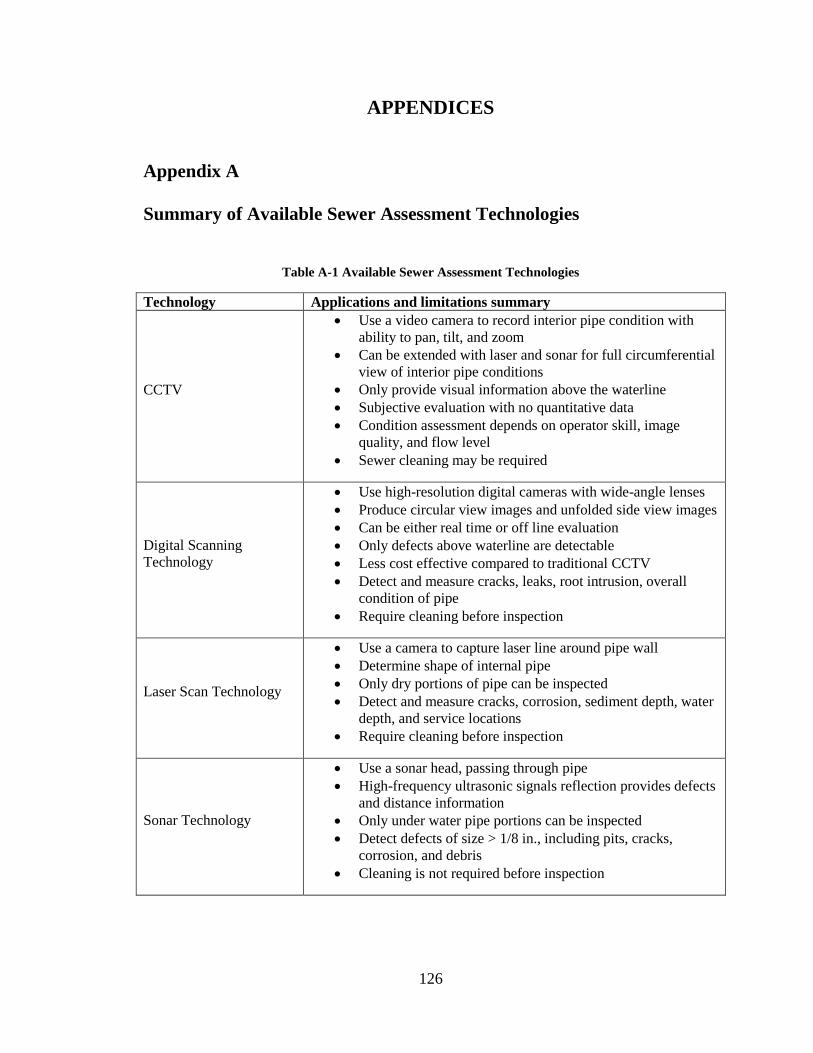
126
APPENDICES
Appendix A
Summary of Available Sewer Assessment Technologies
Table A-1 Available Sewer Assessment Technologies
Technology Applications and limitations summary
CCTV
Use a video camera to record interior pipe condition with
ability to pan, tilt, and zoom
Can be extended with laser and sonar for full circumferential
view of interior pipe conditions
Only provide visual information above the waterline
Subjective evaluation with no quantitative data
Condition assessment depends on operator skill, image
quality, and flow level
Sewer cleaning may be required
Digital Scanning
Technology
Use high-resolution digital cameras with wide-angle lenses
Produce circular view images and unfolded side view images
Can be either real time or off line evaluation
Only defects above waterline are detectable
Less cost effective compared to traditional CCTV
Detect and measure cracks, leaks, root intrusion, overall
condition of pipe
Require cleaning before inspection
Laser Scan Technology
Use a camera to capture laser line around pipe wall
Determine shape of internal pipe
Only dry portions of pipe can be inspected
Detect and measure cracks, corrosion, sediment depth, water
depth, and service locations
Require cleaning before inspection
Sonar Technology
Use a sonar head, passing through pipe
High-frequency ultrasonic signals reflection provides defects
and distance information
Only under water pipe portions can be inspected
Detect defects of size > 1/8 in., including pits, cracks,
corrosion, and debris
Cleaning is not required before inspection
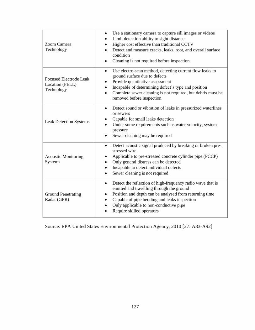
127
Zoom Camera
Technology
Use a stationary camera to capture sill images or videos
Limit detection ability to sight distance
Higher cost effective than traditional CCTV
Detect and measure cracks, leaks, root, and overall surface
condition
Cleaning is not required before inspection
Focused Electrode Leak
Location (FELL)
Technology
Use electro-scan method, detecting current flow leaks to
ground surface due to defects
Provide quantitative assessment
Incapable of determining defect’s type and position
Complete sewer cleaning is not required, but debris must be
removed before inspection
Leak Detection Systems
Detect sound or vibration of leaks in pressurized waterlines
or sewers
Capable for small leaks detection
Under some requirements such as water velocity, system
pressure
Sewer cleaning may be required
Acoustic Monitoring
Systems
Detect acoustic signal produced by breaking or broken pre-
stressed wire
Applicable to pre-stressed concrete cylinder pipe (PCCP)
Only general distress can be detected
Incapable to detect individual defects
Sewer cleaning is not required
Ground Penetrating
Radar (GPR)
Detect the reflection of high-frequency radio wave that is
emitted and travelling through the ground
Position and depth can be analysed from returning time
Capable of pipe bedding and leaks inspection
Only applicable to non-conductive pipe
Require skilled operators
Source: EPA United States Environmental Protection Agency, 2010 [27: A83-A92]
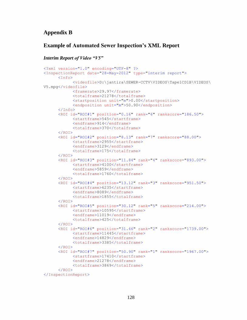
128
Appendix B
Example of Automated Sewer Inspection’s XML Report
Interim Report of Video “V5”
<?xml version="1.0" encoding="UTF-8" ?>
<InspectionReport date="28-May-2012" type="interim report">
<Info>
<videofile>D:\jantira\SEWER-CCTV\VIDEOS\Tape1CD1B\VIDEOS\
V5.mpg</videofile>
<framerate>29.97</framerate>
<totalframe>21278</totalframe>
<startposition unit="m">0.00</startposition>
<endposition unit="m">50.90</endposition>
</Info>
<ROI id="ROI#1" position="0.16" rank="6" rankscore="186.50">
<startframe>545</startframe>
<endframe>914</endframe>
<totalframe>370</totalframe>
</ROI>
<ROI id="ROI#2" position="8.13" rank="7" rankscore="88.00">
<startframe>2955</startframe>
<endframe>3129</endframe>
<totalframe>175</totalframe>
</ROI>
<ROI id="ROI#3" position="11.84" rank="4" rankscore="893.00">
<startframe>4100</startframe>
<endframe>5859</endframe>
<totalframe>1760</totalframe>
</ROI>
<ROI id="ROI#4" position="13.12" rank="3" rankscore="951.50">
<startframe>6235</startframe>
<endframe>8089</endframe>
<totalframe>1855</totalframe>
</ROI>
<ROI id="ROI#5" position="30.12" rank="5" rankscore="214.00">
<startframe>10595</startframe>
<endframe>11019</endframe>
<totalframe>425</totalframe>
</ROI>
<ROI id="ROI#6" position="31.46" rank="2" rankscore="1739.00">
<startframe>11445</startframe>
<endframe>14829</endframe>
<totalframe>3385</totalframe>
</ROI>
<ROI id="ROI#7" position="50.90" rank="1" rankscore="1967.00">
<startframe>17410</startframe>
<endframe>21278</endframe>
<totalframe>3869</totalframe>
</ROI>
</InspectionReport>
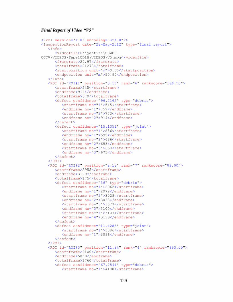
129
Final Report of Video “V5”
<?xml version="1.0" encoding="utf-8"?>
<InspectionReport date="28-May-2012" type="final report">
<Info>
<videofile>D:\jantira\SEWER-
CCTV\VIDEOS\Tape1CD1B\VIDEOS\V5.mpg</videofile>
<framerate>29.97</framerate>
<totalframe>21278</totalframe>
<startposition unit="m">0.00</startposition>
<endposition unit="m">50.90</endposition>
</Info>
<ROI id="ROI#1" position="0.16" rank="6" rankscore="186.50">
<startframe>545</startframe>
<endframe>914</endframe>
<totalframe>370</totalframe>
<defect confidence="96.2162" type="debris">
<startframe no="1">545</startframe>
<endframe no="1">759</endframe>
<startframe no="2">773</startframe>
<endframe no="2">914</endframe>
</defect>
<defect confidence="15.1351" type="joint">
<startframe no="1">586</startframe>
<endframe no="1">595</endframe>
<startframe no="2">626</startframe>
<endframe no="2">653</endframe>
<startframe no="3">660</startframe>
<endframe no="3">675</endframe>
</defect>
</ROI>
<ROI id="ROI#2" position="8.13" rank="7" rankscore="88.00">
<startframe>2955</startframe>
<endframe>3129</endframe>
<totalframe>175</totalframe>
<defect confidence="36" type="debris">
<startframe no="1">2962</startframe>
<endframe no="1">2972</endframe>
<startframe no="2">3028</startframe>
<endframe no="2">3038</endframe>
<startframe no="3">3077</startframe>
<endframe no="3">3100</endframe>
<startframe no="4">3107</startframe>
<endframe no="4">3119</endframe>
</defect>
<defect confidence="11.4286" type="joint">
<startframe no="1">3086</startframe>
<endframe no="1">3096</endframe>
</defect>
</ROI>
<ROI id="ROI#3" position="11.84" rank="4" rankscore="893.00">
<startframe>4100</startframe>
<endframe>5859</endframe>
<totalframe>1760</totalframe>
<defect confidence="67.7841" type="debris">
<startframe no="1">4100</startframe>
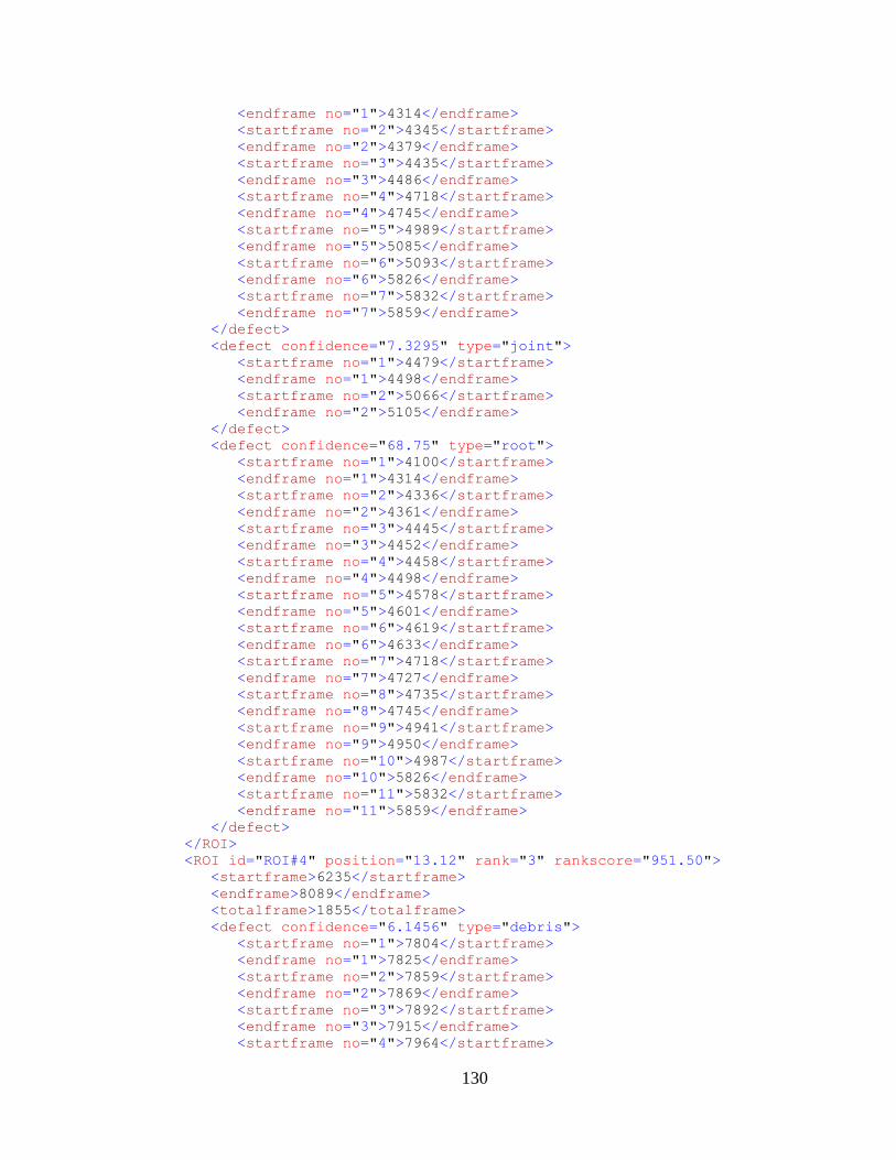
130
<endframe no="1">4314</endframe>
<startframe no="2">4345</startframe>
<endframe no="2">4379</endframe>
<startframe no="3">4435</startframe>
<endframe no="3">4486</endframe>
<startframe no="4">4718</startframe>
<endframe no="4">4745</endframe>
<startframe no="5">4989</startframe>
<endframe no="5">5085</endframe>
<startframe no="6">5093</startframe>
<endframe no="6">5826</endframe>
<startframe no="7">5832</startframe>
<endframe no="7">5859</endframe>
</defect>
<defect confidence="7.3295" type="joint">
<startframe no="1">4479</startframe>
<endframe no="1">4498</endframe>
<startframe no="2">5066</startframe>
<endframe no="2">5105</endframe>
</defect>
<defect confidence="68.75" type="root">
<startframe no="1">4100</startframe>
<endframe no="1">4314</endframe>
<startframe no="2">4336</startframe>
<endframe no="2">4361</endframe>
<startframe no="3">4445</startframe>
<endframe no="3">4452</endframe>
<startframe no="4">4458</startframe>
<endframe no="4">4498</endframe>
<startframe no="5">4578</startframe>
<endframe no="5">4601</endframe>
<startframe no="6">4619</startframe>
<endframe no="6">4633</endframe>
<startframe no="7">4718</startframe>
<endframe no="7">4727</endframe>
<startframe no="8">4735</startframe>
<endframe no="8">4745</endframe>
<startframe no="9">4941</startframe>
<endframe no="9">4950</endframe>
<startframe no="10">4987</startframe>
<endframe no="10">5826</endframe>
<startframe no="11">5832</startframe>
<endframe no="11">5859</endframe>
</defect>
</ROI>
<ROI id="ROI#4" position="13.12" rank="3" rankscore="951.50">
<startframe>6235</startframe>
<endframe>8089</endframe>
<totalframe>1855</totalframe>
<defect confidence="6.1456" type="debris">
<startframe no="1">7804</startframe>
<endframe no="1">7825</endframe>
<startframe no="2">7859</startframe>
<endframe no="2">7869</endframe>
<startframe no="3">7892</startframe>
<endframe no="3">7915</endframe>
<startframe no="4">7964</startframe>
131
<endframe no="4">7979</endframe>
<startframe no="5">8006</startframe>
<endframe no="5">8027</endframe>
</defect>
<defect confidence="0.97035" type="joint">
<startframe no="1">8006</startframe>
<endframe no="1">8021</endframe>
</defect>
<defect confidence="3.8814" type="root">
<startframe no="1">7837</startframe>
<endframe no="1">7848</endframe>
<startframe no="2">7854</startframe>
<endframe no="2">7917</endframe>
</defect>
</ROI>
<ROI id="ROI#5" position="30.12" rank="5" rankscore="214.00">
<startframe>10595</startframe>
<endframe>11019</endframe>
<totalframe>425</totalframe>
<defect confidence="95.0588" type="debris">
<startframe no="1">10600</startframe>
<endframe no="1">10952</endframe>
<startframe no="2">10957</startframe>
<endframe no="2">11019</endframe>
</defect>
<defect confidence="21.6471" type="joint">
<startframe no="1">10604</startframe>
<endframe no="1">10626</endframe>
<startframe no="2">10739</startframe>
<endframe no="2">10751</endframe>
<startframe no="3">10872</startframe>
<endframe no="3">10880</endframe>
<startframe no="4">10886</startframe>
<endframe no="4">10897</endframe>
<startframe no="5">11010</startframe>
<endframe no="5">11019</endframe>
</defect>
<defect confidence="13.1765" type="root">
<startframe no="1">10871</startframe>
<endframe no="1">10932</endframe>
</defect>
</ROI>
<ROI id="ROI#6" position="31.46" rank="2" rankscore="1739.00">
<startframe>11445</startframe>
<endframe>14829</endframe>
<totalframe>3385</totalframe>
<defect confidence="87.4151" type="debris">
<startframe no="1">11445</startframe>
<endframe no="1">13774</endframe>
<startframe no="2">13787</startframe>
<endframe no="2">14003</endframe>
<startframe no="3">14013</startframe>
<endframe no="3">14032</endframe>
<startframe no="4">14079</startframe>
<endframe no="4">14094</endframe>
<startframe no="5">14099</startframe>
<endframe no="5">14119</endframe>
132
<startframe no="6">14141</startframe>
<endframe no="6">14152</endframe>
<startframe no="7">14184</startframe>
<endframe no="7">14488</endframe>
<startframe no="8">14493</startframe>
<endframe no="8">14526</endframe>
<startframe no="9">14535</startframe>
<endframe no="9">14586</endframe>
<startframe no="10">14591</startframe>
<endframe no="10">14608</endframe>
<startframe no="11">14636</startframe>
<endframe no="11">14683</endframe>
<startframe no="12">14771</startframe>
<endframe no="12">14829</endframe>
</defect>
<defect confidence="12.2304" type="joint">
<startframe no="1">11457</startframe>
<endframe no="1">11469</endframe>
<startframe no="2">11722</startframe>
<endframe no="2">11730</endframe>
<startframe no="3">12108</startframe>
<endframe no="3">12116</endframe>
<startframe no="4">12136</startframe>
<endframe no="4">12185</endframe>
<startframe no="5">12191</startframe>
<endframe no="5">12221</endframe>
<startframe no="6">12231</startframe>
<endframe no="6">12248</endframe>
<startframe no="7">12285</startframe>
<endframe no="7">12311</endframe>
<startframe no="8">12435</startframe>
<endframe no="8">12481</endframe>
<startframe no="9">12509</startframe>
<endframe no="9">12600</endframe>
<startframe no="10">12607</startframe>
<endframe no="10">12676</endframe>
<startframe no="11">12711</startframe>
<endframe no="11">12727</endframe>
<startframe no="12">14641</startframe>
<endframe no="12">14652</endframe>
</defect>
<defect confidence="14.4756" type="root">
<startframe no="1">11778</startframe>
<endframe no="1">11830</endframe>
<startframe no="2">11881</startframe>
<endframe no="2">11913</endframe>
<startframe no="3">12041</startframe>
<endframe no="3">12054</endframe>
<startframe no="4">12781</startframe>
<endframe no="4">12821</endframe>
<startframe no="5">12905</startframe>
<endframe no="5">12917</endframe>
<startframe no="6">12923</startframe>
<endframe no="6">12978</endframe>
<startframe no="7">12990</startframe>
<endframe no="7">13079</endframe>
<startframe no="8">13084</startframe>
133
<endframe no="8">13146</endframe>
<startframe no="9">13164</startframe>
<endframe no="9">13177</endframe>
<startframe no="10">13197</startframe>
<endframe no="10">13231</endframe>
<startframe no="11">13237</startframe>
<endframe no="11">13246</endframe>
<startframe no="12">13252</startframe>
<endframe no="12">13284</endframe>
<startframe no="13">13290</startframe>
<endframe no="13">13298</endframe>
<startframe no="14">13308</startframe>
<endframe no="14">13329</endframe>
<startframe no="15">13334</startframe>
<endframe no="15">13358</endframe>
</defect>
</ROI>
<ROI id="ROI#7" position="50.90" rank="1" rankscore="1967.00">
<startframe>17410</startframe>
<endframe>21278</endframe>
<totalframe>3869</totalframe>
<defect confidence="90.5919" type="debris">
<startframe no="1">17410</startframe>
<endframe no="1">17632</endframe>
<startframe no="2">17637</startframe>
<endframe no="2">17739</endframe>
<startframe no="3">17776</startframe>
<endframe no="3">17807</endframe>
<startframe no="4">17813</startframe>
<endframe no="4">17867</endframe>
<startframe no="5">17874</startframe>
<endframe no="5">17901</endframe>
<startframe no="6">17906</startframe>
<endframe no="6">17923</endframe>
<startframe no="7">17980</startframe>
<endframe no="7">19003</endframe>
<startframe no="8">19008</startframe>
<endframe no="8">19018</endframe>
<startframe no="9">19042</startframe>
<endframe no="9">19385</endframe>
<startframe no="10">19390</startframe>
<endframe no="10">20197</endframe>
<startframe no="11">20234</startframe>
<endframe no="11">20465</endframe>
<startframe no="12">20482</startframe>
<endframe no="12">20498</endframe>
<startframe no="13">20503</startframe>
<endframe no="13">20622</endframe>
<startframe no="14">20627</startframe>
<endframe no="14">20708</endframe>
<startframe no="15">20736</startframe>
<endframe no="15">21278</endframe>
</defect>
<defect confidence="10.8555" type="joint">
<startframe no="1">17469</startframe>
<endframe no="1">17493</endframe>
<startframe no="2">17499</startframe>

134
<endframe no="2">17526</endframe>
<startframe no="3">17537</startframe>
<endframe no="3">17559</endframe>
<startframe no="4">17564</startframe>
<endframe no="4">17581</endframe>
<startframe no="5">17777</startframe>
<endframe no="5">17789</endframe>
<startframe no="6">17805</startframe>
<endframe no="6">17816</endframe>
<startframe no="7">17834</startframe>
<endframe no="7">17851</endframe>
<startframe no="8">18031</startframe>
<endframe no="8">18042</endframe>
<startframe no="9">19789</startframe>
<endframe no="9">19867</endframe>
<startframe no="10">19882</startframe>
<endframe no="10">19915</endframe>
<startframe no="11">19933</startframe>
<endframe no="11">19945</endframe>
<startframe no="12">19950</startframe>
<endframe no="12">19976</endframe>
<startframe no="13">19983</startframe>
<endframe no="13">20006</endframe>
<startframe no="14">20399</startframe>
<endframe no="14">20440</endframe>
<startframe no="15">20772</startframe>
<endframe no="15">20800</endframe>
<startframe no="16">20808</startframe>
<endframe no="16">20819</endframe>
</defect>
<defect confidence="6.7976" type="root">
<startframe no="1">17452</startframe>
<endframe no="1">17462</endframe>
<startframe no="2">17572</startframe>
<endframe no="2">17586</endframe>
<startframe no="3">18534</startframe>
<endframe no="3">18566</endframe>
<startframe no="4">18573</startframe>
<endframe no="4">18582</endframe>
<startframe no="5">18592</startframe>
<endframe no="5">18602</endframe>
<startframe no="6">19413</startframe>
<endframe no="6">19423</endframe>
<startframe no="7">19499</startframe>
<endframe no="7">19645</endframe>
<startframe no="8">20069</startframe>
<endframe no="8">20088</endframe>
<startframe no="9">20843</startframe>
<endframe no="9">20853</endframe>
</defect>
</ROI>
</InspectionReport>
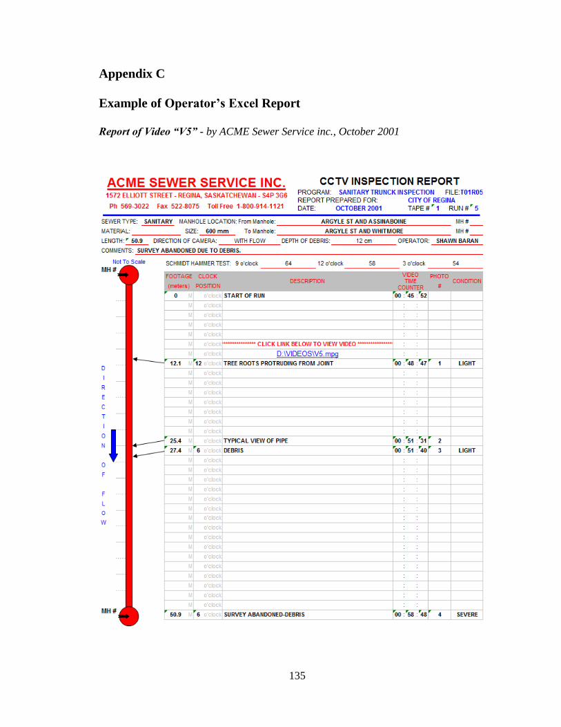
135
Appendix C
Example of Operator’s Excel Report
Report of Video “V5” - by ACME Sewer Service inc., October 2001

136