Embed Size (px)
Citation preview
Automated 3D Crack Growth Simulation 1 November 18, 2003
Automated 3D Crack Growth Simulation
B.J. CARTER, P.A. WAWRZYNEK, and A.R. INGRAFFEA
Cornell Fracture Group, 641 Rhodes Hall,
Cornell University, Ithaca, NY, USA 14853
SUMMARY
Automated simulation of arbitrary, non-planar, 3D crack growth in real-life engineered
structures requires two key components: crack representation and crack growth mechanics.
A model environment for representing the evolving 3D crack geometry and for testing
various crack growth mechanics is presented. Reference is made to a specific implementation
of the model, called FRANC3D. Computational geometry and topology are used to represent
the evolution of crack growth in a structure. Current 3D crack growth mechanics are
insufficient; however, the model allows for the implementation of new mechanics. A
specific numerical analysis program is not an intrinsic part of the model; i.e., finite and
boundary elements are both supported. For demonstration purposes, a 3D hypersingular
boundary element code is used for two example simulations. The simulations support the
conclusion that automatic propagation of a 3D crack in a real-life structure is feasible.
Automated simulation lessens the tedious and time-consuming operations that are usually
associated with crack growth analyses. Specifically, modifications to the geometry of the
structure due to crack growth, re-meshing of the modified portion of the structure after crack
growth, and re-application of boundary conditions proceeds without user intervention.
KEYWORDS: three-dimensional, fracture, fatigue simulation
Automated 3D Crack Growth Simulation 2 November 18, 2003
1. INTRODUCTION
Crack growth simulation is the process of modeling crack evolution in a structure through
time or with increasing load. This encompasses all aspects of the modeling process from
initial data preparation to visualization of results, leading to prediction of crack growth and
evaluation of structural integrity. Crack growth simulations are common in many fields of
engineering: microscopic cracks in single crystals1, fatigue cracks in aircraft structures2, and
cracking in large concrete dams3 are just a few examples.
Cracks can affect the integrity and the performance of an engineered structure. Although
cracks can never be eliminated, their detrimental effects at least should be mitigated. To
accomplish this, some form of analysis is needed to determine if, when, and how cracking
evolves. In many cases, back-of-the-envelope calculations are sufficient to decide whether a
crack will grow and whether the structure is safe. In some cases, however, it is necessary to
perform detailed, fully three-dimensional, numerical simulations.
In many engineered structures, observed cracks are non-planar 3D features that nucleate from
areas of high stress concentrations in geometrically complex regions of the structure. Despite
the fact that many observed cracks are truly 3D, they often are idealized as planar 3D or
simply as 2D features. Although this drastically simplifies the simulation, the accuracy of the
predictions based on these idealizations generally has not been well characterized. To
quantify the predictions from these idealized models, it is desirable and necessary to have a
truly-3D crack growth simulator. In addition, where such idealizations are poor or
impossible, detailed 3D simulations can be performed forthwith.
Most commercial stress analysis programs are not suitable for the purpose of simulating 3D
crack growth. Although many commercial programs can perform an accurate stress analysis
of a cracked structure, the subsequent propagation of the crack usually is not a simple
Automated 3D Crack Growth Simulation 3 November 18, 2003
process. 3D fracture simulations have been described in the literature4-11; most of these
concentrate on the numerical analysis, neglecting the issues of representation and automated
propagation. In fact, many of the 3D fracture simulations are really pseudo-3D, as the
modeled crack surface remains planar.
To model an evolving crack efficiently and automatically in a complex 3D structure, one
requires two integral components in a simulator: crack representation and crack growth
mechanics. Representation includes the details of storing the geometry of a cracked body in a
computer and updating the geometric description to reflect crack growth; this includes both
the real geometry and the mathematical representation, i.e., the mesh. Mechanics includes
stress analysis, extraction of relevant crack growth parameters, and determination of the
shape, extent, and direction of crack growth. These two components form the basis for
modeling crack evolution.
A conceptual model of a software framework that allows efficient and automatic simulation
of 3D crack propagation is presented. The representational aspects of crack growth
simulation and the components of the conceptual model are discussed in detail using simple
examples to illustrate the key points. Brief discussions of the mechanics of crack growth are
included when appropriate. A specific implementation, called FRANC3D12-14, is used to
predict stress intensity factors for an evolving 3D crack in two different structures: a non-
planar angled crack in a beam under four-point bending and a planar crack in a rotating
turbine disk.
Automated 3D Crack Growth Simulation 4 November 18, 2003
2. A CONCEPTUAL MODEL OF CRACK GROWTH SIMULATION
Crack growth simulation is an incremental process, where a series of steps is repeated for a
progression of models. Each increment of the simulation relies on previously computed
results and represents one crack configuration. There are four primary collections of data or
databases required for each increment. The first is the representational database, denoted Ri ,
where the subscript identifies the increment number. The representational database contains
a description of the solid model geometry, including the cracks, the boundary conditions, and
the material properties. The representational database is transformed by a discretization
process D to a stress analysis database Ai . The discretization process includes a meshing
function M.
D(Ri ,M(Ri ))� Ai (1)
The analysis database contains a complete, but approximate description of the body, suitable
for input to a solution procedure S, often a finite or boundary element stress analysis
program. The solution procedure S is used to transform the analysis database Ai to an
equilibrium database E i which consists of field variables, such as displacements and stresses,
that define the equilibrium solution. The equilibrium solution should contain field variables
and material state information, and in the context of a crack growth simulation, should also
contain values for stress-intensity factors or other fracture parameters F i for all crack fronts.
S(Ai )� Ei , F i (2)
By means of an update function U, E i in conjunction with Ri is used to create a new
representational model Ri +1 , which includes the crack growth increment. The crack growth
function C, which is part of U, determines the direction and extent of the crack growth
increment.
U E i , Ri ,C(F i )( )� Ri +1 (3)
This sequence of operations, as shown in Figure 1, is repeated until a suitable termination
condition is reached. Results of such a simulation might include one or more of the
following: a final crack geometry, a loading versus crack size history, a crack opening
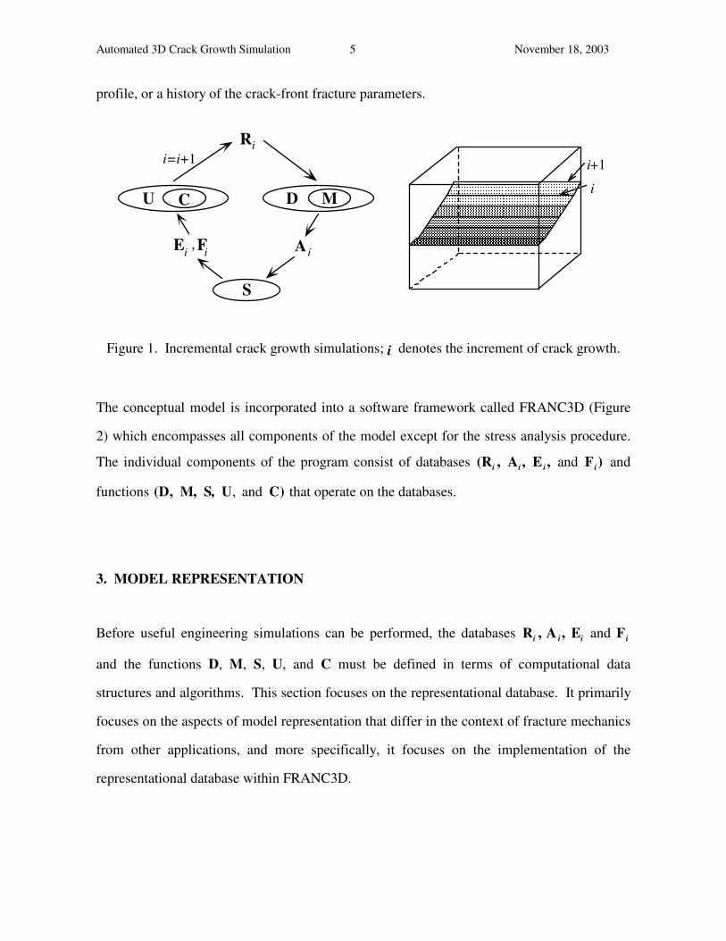
Automated 3D Crack Growth Simulation 5 November 18, 2003
profile, or a history of the crack-front fracture parameters.
U C
Ri
AiEi Fi,
i
i+1i=i+1
S
MD
Figure 1. Incremental crack growth simulations; i denotes the increment of crack growth.
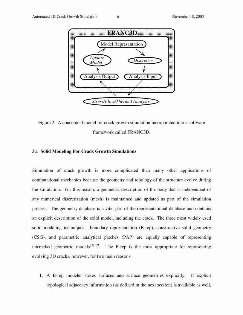
The conceptual model is incorporated into a software framework called FRANC3D (Figure
2) which encompasses all components of the model except for the stress analysis procedure.
The individual components of the program consist of databases (Ri , Ai , E i , and F i) and
functions (D, M, S, U, and C) that operate on the databases.
3. MODEL REPRESENTATION
Before useful engineering simulations can be performed, the databases Ri , A i , Ei and F i
and the functions D, M, S, U, and C must be defined in terms of computational data
structures and algorithms. This section focuses on the representational database. It primarily
focuses on the aspects of model representation that differ in the context of fracture mechanics
from other applications, and more specifically, it focuses on the implementation of the
representational database within FRANC3D.
Automated 3D Crack Growth Simulation 6 November 18, 2003
Stress/Flow/Thermal Analysis
Model Representation
Discretize
FRANC3D
Analysis Input
UpdateModel
Analysis Output
Figure 2. A conceptual model for crack growth simulation incorporated into a software
framework called FRANC3D.
3.1 Solid Modeling For Crack Growth Simulations
Simulation of crack growth is more complicated than many other applications of
computational mechanics because the geometry and topology of the structure evolve during
the simulation. For this reason, a geometric description of the body that is independent of
any numerical discretization (mesh) is maintained and updated as part of the simulation
process. The geometry database is a vital part of the representational database and contains
an explicit description of the solid model, including the crack. The three most widely used
solid modeling techniques: boundary representation (B-rep), constructive solid geometry
(CSG), and parametric analytical patches (PAP) are equally capable of representing
uncracked geometric models15-17. The B-rep is the most appropriate for representing
evolving 3D cracks, however, for two main reasons.
1. A B-rep modeler stores surfaces and surface geometries explicitly. If explicit
topological adjacency information (as defined in the next section) is available as well,
Automated 3D Crack Growth Simulation 7 November 18, 2003
two topologically distinct surfaces can share a common geometric description. A
crack represents such a configuration. A B-rep modeler uses only the surface
topology and geometry to represent the three-dimensional solid structure. A crack
actually consists of two surfaces that have the same geometric description and both of
these surfaces form part of the solid model boundary.
2. Both 3D solids and dimensionally degenerate forms, such as plates or shells can be
represented equally well with a B-rep modeler. Plates and shells are represented
using a single topological surface to represent each plate/shell surface. This means
that crack growth can be modeled in both solid and thin shell structures using the
same software framework. Note that cracks in shells are mentioned here, but the
primary focus is on 3D solid structures.
3.2 Computational Topology as a Framework for Crack Growth Simulation
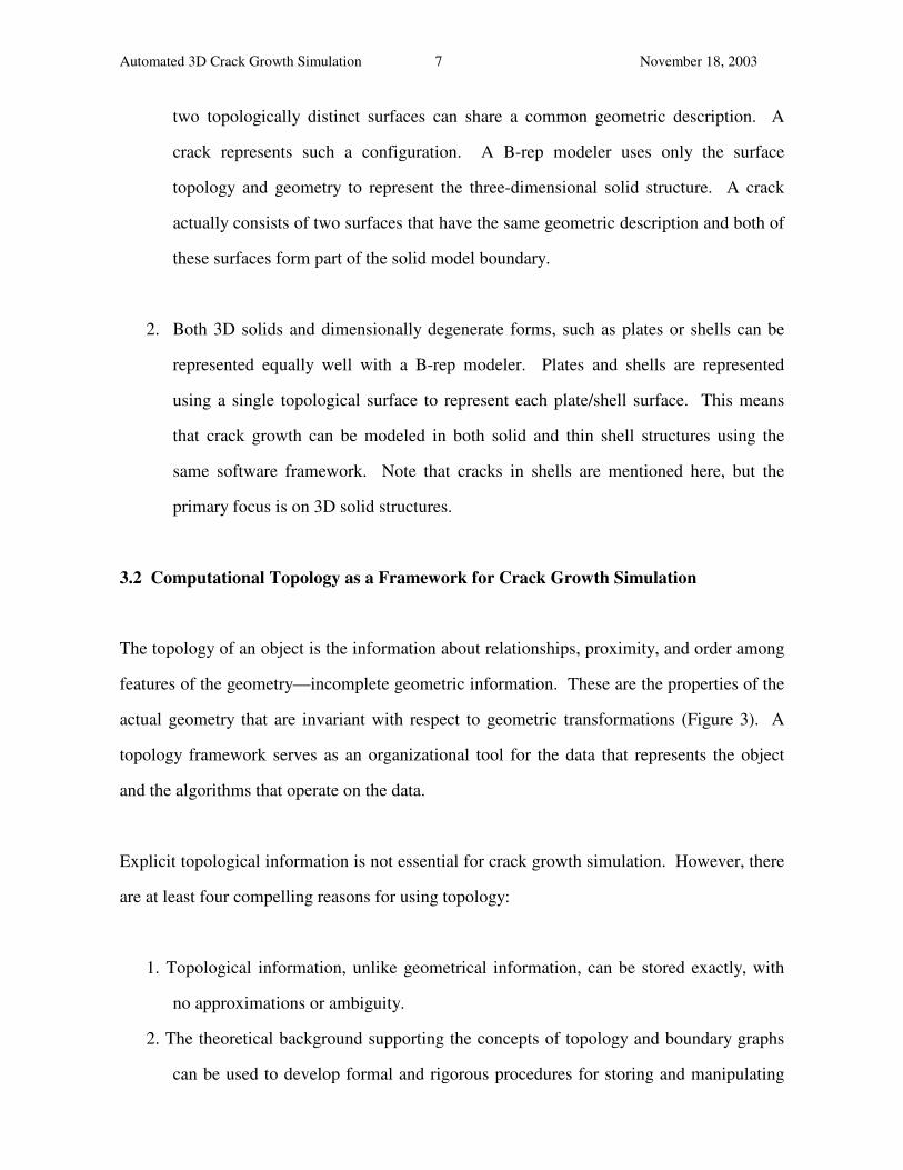
The topology of an object is the information about relationships, proximity, and order among
features of the geometry—incomplete geometric information. These are the properties of the
actual geometry that are invariant with respect to geometric transformations (Figure 3). A
topology framework serves as an organizational tool for the data that represents the object
and the algorithms that operate on the data.
Explicit topological information is not essential for crack growth simulation. However, there
are at least four compelling reasons for using topology:
1. Topological information, unlike geometrical information, can be stored exactly, with
no approximations or ambiguity.
2. The theoretical background supporting the concepts of topology and boundary graphs
can be used to develop formal and rigorous procedures for storing and manipulating
Automated 3D Crack Growth Simulation 8 November 18, 2003
these types of data15,16,18.
3. Any topological configuration can represent an infinite number of geometrical
configurations.
4. During crack propagation, the geometry of the structure changes with each crack
increment whereas the topology generally changes less frequently.
x
y
z
topology geometrytied to
vertex
edge
face
Figure 3. Relationship between topology and geometry; a topological entity can have any
number of geometric descriptions.
Prior investigations into the use of data structures for crack propagation simulations19,20
showed that topological databases are a convenient and powerful organizing agent. Topology
allows one to build an efficient system for interactive modeling while hiding the complexities
in manipulating the data. Explicit topological information is used herein as a framework for
Ri and aids in implementation of the functions D and U. Topological entities (such as
vertices, edges, and faces) serve as the principal elements of the database with geometrical
descriptions and other attributes (such as boundary conditions and material properties)
accessed through the topological entities.
Several topological data structures have been proposed for manifold objects. These include:
the winged-edge, the modified winged-edge, the face-edge, the vertex-edge, and the half-edge
Automated 3D Crack Growth Simulation 9 November 18, 2003
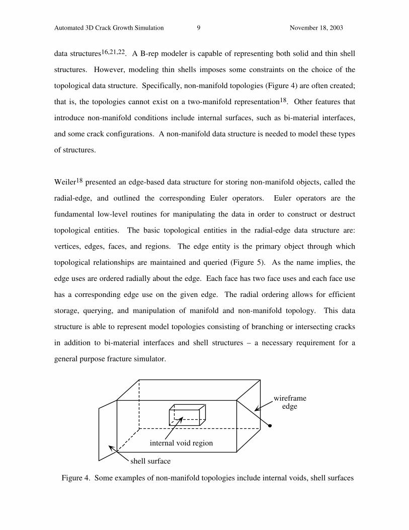
data structures16,21,22. A B-rep modeler is capable of representing both solid and thin shell
structures. However, modeling thin shells imposes some constraints on the choice of the
topological data structure. Specifically, non-manifold topologies (Figure 4) are often created;
that is, the topologies cannot exist on a two-manifold representation18. Other features that
introduce non-manifold conditions include internal surfaces, such as bi-material interfaces,
and some crack configurations. A non-manifold data structure is needed to model these types
of structures.
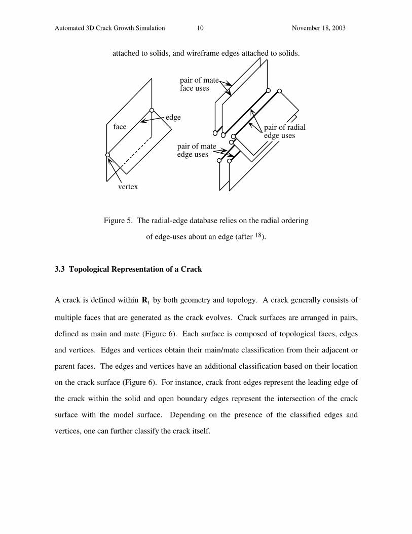
Weiler18 presented an edge-based data structure for storing non-manifold objects, called the
radial-edge, and outlined the corresponding Euler operators. Euler operators are the
fundamental low-level routines for manipulating the data in order to construct or destruct
topological entities. The basic topological entities in the radial-edge data structure are:
vertices, edges, faces, and regions. The edge entity is the primary object through which
topological relationships are maintained and queried (Figure 5). As the name implies, the
edge uses are ordered radially about the edge. Each face has two face uses and each face use
has a corresponding edge use on the given edge. The radial ordering allows for efficient
storage, querying, and manipulation of manifold and non-manifold topology. This data
structure is able to represent model topologies consisting of branching or intersecting cracks
in addition to bi-material interfaces and shell structures – a necessary requirement for a
general purpose fracture simulator.
shell surface
internal void region
wireframeedge
Figure 4. Some examples of non-manifold topologies include internal voids, shell surfaces
Automated 3D Crack Growth Simulation 10 November 18, 2003
attached to solids, and wireframe edges attached to solids.
faceedge
pair of mateface uses
pair of mateedge uses
pair of radialedge uses
vertex
Figure 5. The radial-edge database relies on the radial ordering
of edge-uses about an edge (after 18).
3.3 Topological Representation of a Crack
A crack is defined within Ri by both geometry and topology. A crack generally consists of
multiple faces that are generated as the crack evolves. Crack surfaces are arranged in pairs,
defined as main and mate (Figure 6). Each surface is composed of topological faces, edges
and vertices. Edges and vertices obtain their main/mate classification from their adjacent or
parent faces. The edges and vertices have an additional classification based on their location
on the crack surface (Figure 6). For instance, crack front edges represent the leading edge of
the crack within the solid and open boundary edges represent the intersection of the crack
surface with the model surface. Depending on the presence of the classified edges and
vertices, one can further classify the crack itself.
Automated 3D Crack Growth Simulation 11 November 18, 2003
mainsideface
matesideface
frontedge
open boundary edge
tip vertex
front
front
branchedges
branchvertices
tip vertex
mainmate
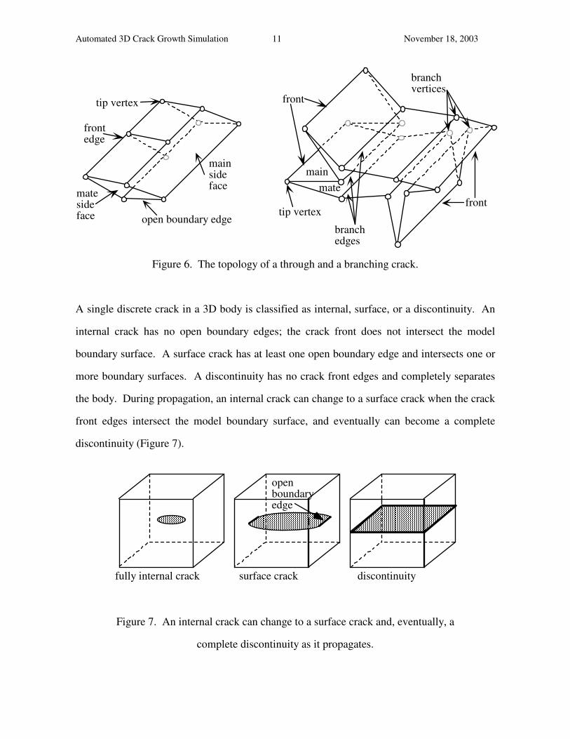
Figure 6. The topology of a through and a branching crack.
A single discrete crack in a 3D body is classified as internal, surface, or a discontinuity. An
internal crack has no open boundary edges; the crack front does not intersect the model
boundary surface. A surface crack has at least one open boundary edge and intersects one or
more boundary surfaces. A discontinuity has no crack front edges and completely separates
the body. During propagation, an internal crack can change to a surface crack when the crack
front edges intersect the model boundary surface, and eventually can become a complete
discontinuity (Figure 7).
fully internal crack surface crack
openboundaryedge
discontinuity
Figure 7. An internal crack can change to a surface crack and, eventually, a
complete discontinuity as it propagates.
Automated 3D Crack Growth Simulation 12 November 18, 2003
3.4 Topological Operations for Crack Nucleation and Propagation
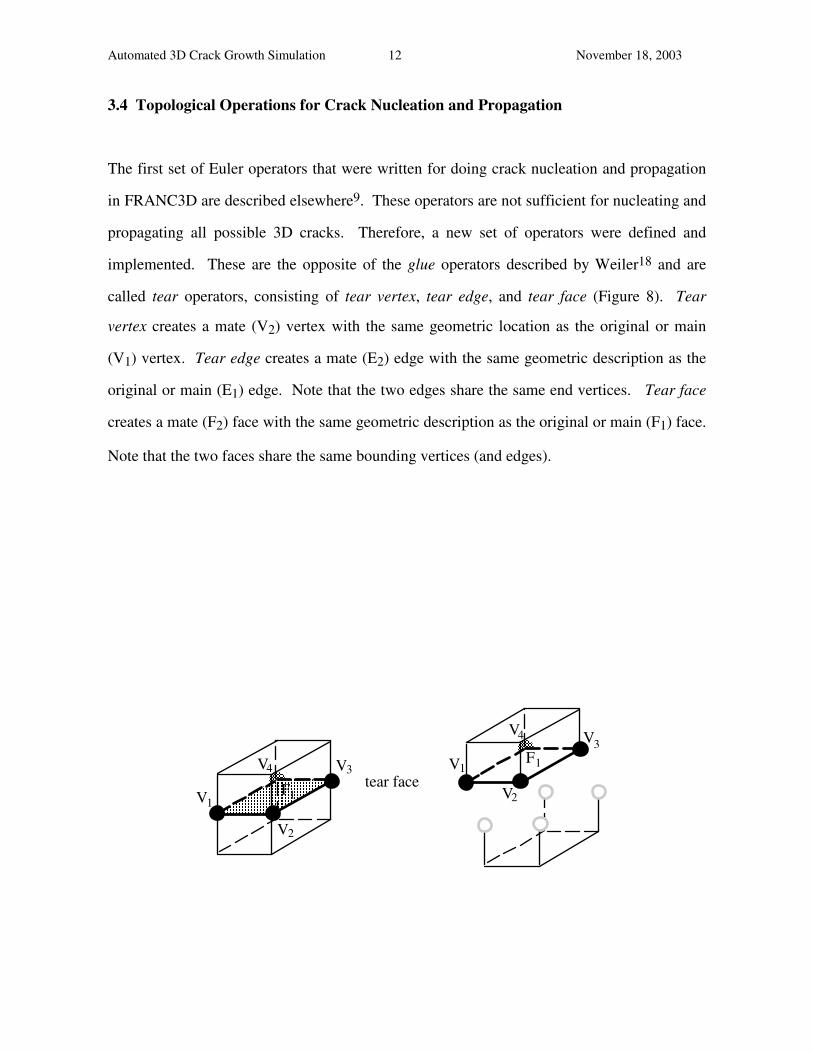
The first set of Euler operators that were written for doing crack nucleation and propagation
in FRANC3D are described elsewhere9. These operators are not sufficient for nucleating and
propagating all possible 3D cracks. Therefore, a new set of operators were defined and
implemented. These are the opposite of the glue operators described by Weiler18 and are
called tear operators, consisting of tear vertex, tear edge, and tear face (Figure 8). Tear
vertex creates a mate (V2) vertex with the same geometric location as the original or main
(V1) vertex. Tear edge creates a mate (E2) edge with the same geometric description as the
original or main (E1) edge. Note that the two edges share the same end vertices. Tear face
creates a mate (F2) face with the same geometric description as the original or main (F1) face.
Note that the two faces share the same bounding vertices (and edges).
V1
V2
V3V4
F1tear face
F1V1
V2
V3V4
F2V1
V2
V3
V4
tear vertex
tear edgeV1
V1V2V2E 1
E 1
E 2V1 V2
V1
V1
V2
Figure 8. The individual tear operators.
Automated 3D Crack Growth Simulation 13 November 18, 2003
The process of creating a 3D crack involves at least the tear face operator and can involve the
other two tear operators as well. The tear operators are used to create all types of cracks
including discontinuities and branch-cracks. Cracks in shell and plate structures can be
created using just the tear edge and tear vertex operators. The complementary glue
operators, glue face, glue edge and glue vertex, have also been implemented so that a crack
can be removed from a structure.
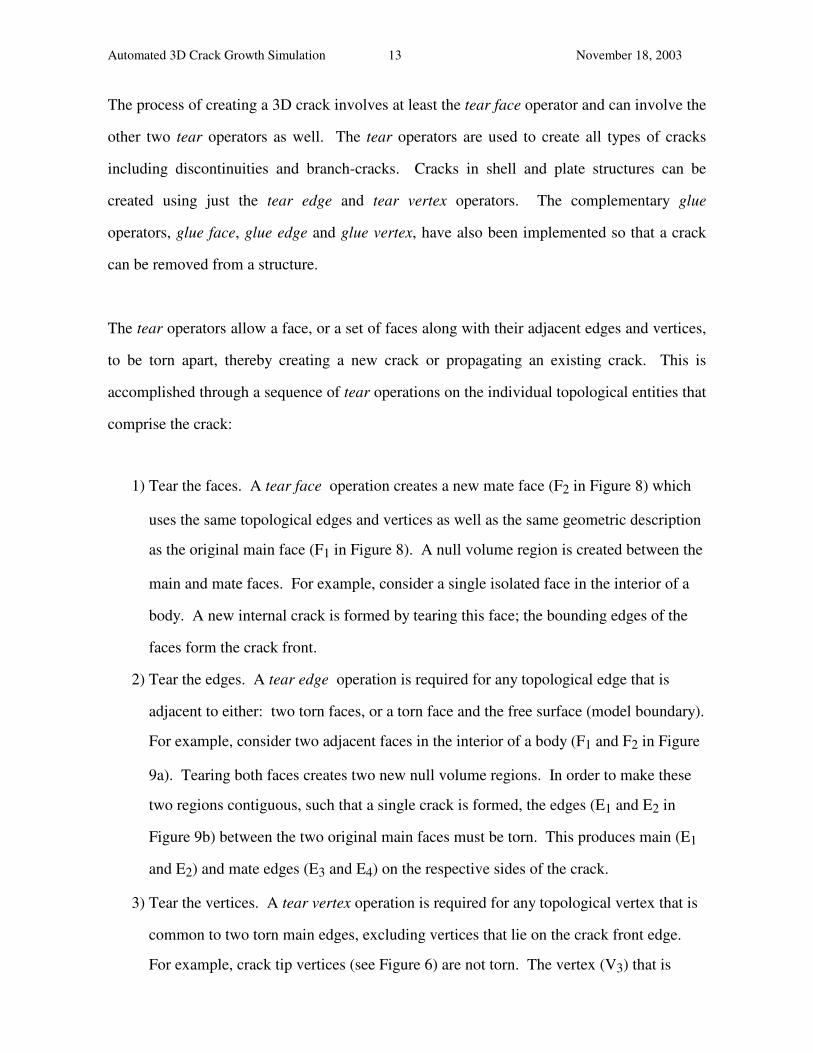
The tear operators allow a face, or a set of faces along with their adjacent edges and vertices,
to be torn apart, thereby creating a new crack or propagating an existing crack. This is
accomplished through a sequence of tear operations on the individual topological entities that
comprise the crack:
1) Tear the faces. A tear face operation creates a new mate face (F2 in Figure 8) which
uses the same topological edges and vertices as well as the same geometric description
as the original main face (F1 in Figure 8). A null volume region is created between the
main and mate faces. For example, consider a single isolated face in the interior of a
body. A new internal crack is formed by tearing this face; the bounding edges of the
faces form the crack front.
2) Tear the edges. A tear edge operation is required for any topological edge that is
adjacent to either: two torn faces, or a torn face and the free surface (model boundary).
For example, consider two adjacent faces in the interior of a body (F1 and F2 in Figure
9a). Tearing both faces creates two new null volume regions. In order to make these
two regions contiguous, such that a single crack is formed, the edges (E1 and E2 in
Figure 9b) between the two original main faces must be torn. This produces main (E1
and E2) and mate edges (E3 and E4) on the respective sides of the crack.
3) Tear the vertices. A tear vertex operation is required for any topological vertex that is
common to two torn main edges, excluding vertices that lie on the crack front edge.
For example, crack tip vertices (see Figure 6) are not torn. The vertex (V3) that is

Automated 3D Crack Growth Simulation 14 November 18, 2003
adjacent to the torn edges (E1 and E2 in Figure 9c) must be torn so that the crack
surfaces are completely separated. Vertices that are not adjacent to two torn edges (V1
and V2) are shared by the main and mate faces.
F3F4
F1F2
F1F2 tear faces
F1 and F2
E1 E2
E1 E2
E3 E4
E1 E2
V1 V3
2V3
2
V1 V
V
V1 V4
2V3
2
V1 V
V
tear edgesE1 and E2
tear vertex V3
(a)
(c)
(b)
Figure 9. The tear operators are used in sequence to create a crack.
3.5 Current Solid Modeling Restrictions in FRANC3D
The previous subsections concentrated on the topological description of the model. A few
words about the geometric properties of the topology are required, especially in relation to the
FRANC3D implementation. Although FRANC3D has some solid modeling capabilities, it is
not a true solid modeler and it has some restrictions and limitations that are important in
terms of describing arbitrary crack nucleation and propagation. These are:
1. Geometric surfaces are represented as planar, triangular Bezier, or quadrilateral bi-
cubic B-spline patches. Patches can have three or four bounding edges. A bounding
Automated 3D Crack Growth Simulation 15 November 18, 2003
edge can be formed from multiple topological edges, however.
2. Geometry edges are either straight lines or cubic B-spline curves. In surface parametric
space, all edges are straight lines.
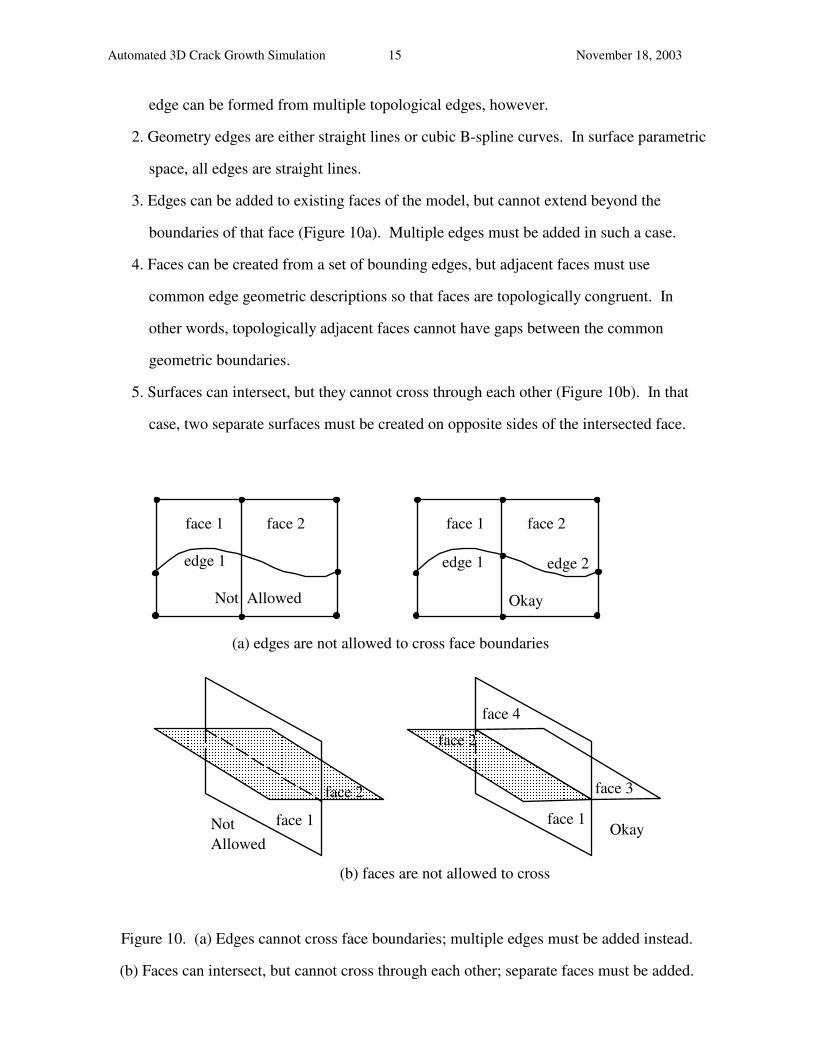
3. Edges can be added to existing faces of the model, but cannot extend beyond the
boundaries of that face (Figure 10a). Multiple edges must be added in such a case.
4. Faces can be created from a set of bounding edges, but adjacent faces must use
common edge geometric descriptions so that faces are topologically congruent. In
other words, topologically adjacent faces cannot have gaps between the common
geometric boundaries.
5. Surfaces can intersect, but they cannot cross through each other (Figure 10b). In that
case, two separate surfaces must be created on opposite sides of the intersected face.
face 1 face 1
face 3
(b) faces are not allowed to cross
face 1 face 2
Not Allowed
edge 1
(a) edges are not allowed to cross face boundaries
NotAllowed
Okay
face 4
face 2
face 2
face 1 face 2
Okay
edge 1 edge 2
Figure 10. (a) Edges cannot cross face boundaries; multiple edges must be added instead.
(b) Faces can intersect, but cannot cross through each other; separate faces must be added.
Automated 3D Crack Growth Simulation 16 November 18, 2003
4. CRACK UPDATE FUNCTION
To represent an evolving crack, a simulator must be capable of both nucleating and
propagating a crack. Crack nucleation consists of placing an initial flaw in the model. Crack
propagation has two components. First, the parameters that govern the crack growth, such as
stress intensity factors, crack growth direction, and amount of extension must be determined.
Second, the topology and geometry must be updated to account for the proper amount of
crack growth. These components are discussed below.
4.1 Techniques for Nucleating Cracks in FRANC3D
Real cracks generally have arbitrary shapes and sizes. Thus, a 3D fracture simulator should
be able to model any crack shape. For many simulations, however, the initial cracks are quite
small with relatively simple geometries. While initial crack geometry is often simple, the
evolutionary geometry can become very complex depending on the stress field and the
geometry of the structure.
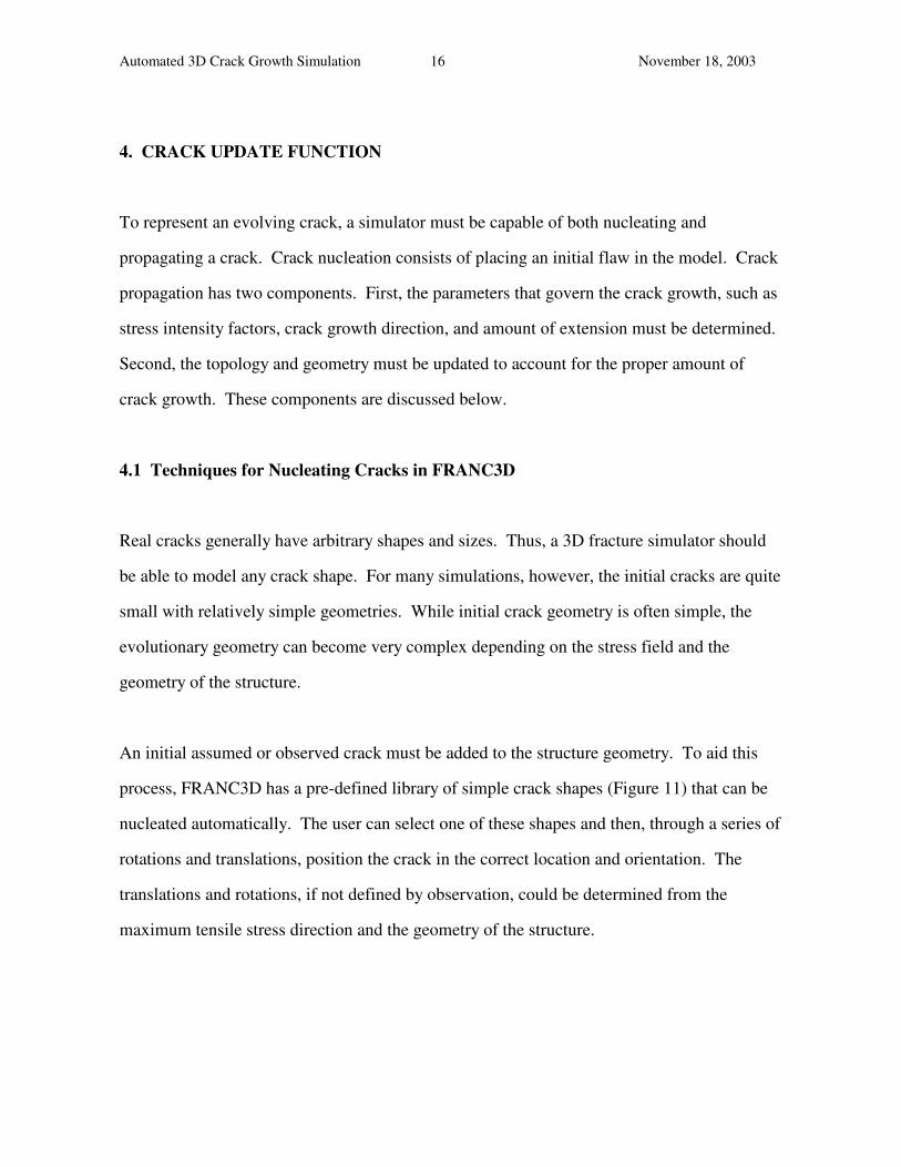
An initial assumed or observed crack must be added to the structure geometry. To aid this
process, FRANC3D has a pre-defined library of simple crack shapes (Figure 11) that can be
nucleated automatically. The user can select one of these shapes and then, through a series of
rotations and translations, position the crack in the correct location and orientation. The
translations and rotations, if not defined by observation, could be determined from the
maximum tensile stress direction and the geometry of the structure.
Automated 3D Crack Growth Simulation 17 November 18, 2003
e.g.: a quarter-ellipticalsurface flaw shape
control point
surfaceedge
internal edge(crack front)
31
2
surface edge
Figure 11. FRANC3D library flaw shapes. Each flaw shape is a planar surface and is
defined by the illustrated boundary edges and control points at the ends of the edges.
Although the library cracks have simple planar geometries, adding a crack to an arbitrary 3D
structure can be quite complicated. First, the control points (Figure 11) that define the ends
of the edges must be located in the model and defined as vertices. New vertices are added if
they do not exist in the model at these locations which implies either splitting a geometry
edge or adding a vertex to a face or to a region. Once all the vertices have been found or
created at all of the control points, the edges are added to the model. The edge geometry as
well as the internal or surface classification is specified by the library data. Edges are added
either directly to surfaces or as wireframe edges to regions. Faces are created from the set of
predefined loops of edges as defined by the library data. The tear operators, as described in
Section 3.4, are used to create a crack from the resulting faces, edges, and vertices.
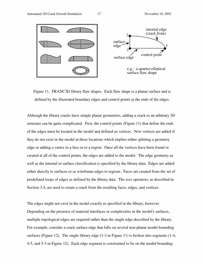
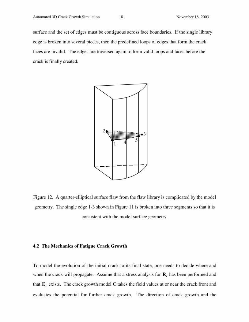
The edges might not exist in the model exactly as specified in the library, however.
Depending on the presence of material interfaces or complexities in the model's surfaces,
multiple topological edges are required rather than the single edge described by the library.
For example, consider a crack surface edge that falls on several non-planar model-bounding
surfaces (Figure 12). The single library edge (1-3 in Figure 11) is broken into segments (1-4,
4-5, and 5-3 in Figure 12). Each edge segment is constrained to lie on the model-bounding
Automated 3D Crack Growth Simulation 18 November 18, 2003
surface and the set of edges must be contiguous across face boundaries. If the single library
edge is broken into several pieces, then the predefined loops of edges that form the crack
faces are invalid. The edges are traversed again to form valid loops and faces before the
crack is finally created.
2
54
3
1
Figure 12. A quarter-elliptical surface flaw from the flaw library is complicated by the model
geometry. The single edge 1-3 shown in Figure 11 is broken into three segments so that it is
consistent with the model surface geometry.
4.2 The Mechanics of Fatigue Crack Growth
To model the evolution of the initial crack to its final state, one needs to decide where and
when the crack will propagate. Assume that a stress analysis for Ri has been performed and
that E i exists. The crack growth model C takes the field values at or near the crack front and
evaluates the potential for further crack growth. The direction of crack growth and the
Automated 3D Crack Growth Simulation 19 November 18, 2003
amount of extension for unique points along the existing crack front defines a set of points in
space that are used to represent the position of the new crack front.
A generally accepted 3D crack growth rule or theory is yet to be developed. The most
common technique for extending a 3D crack is to treat it as a series of 2D plane strain
slices4,23. Although FRANC3D is designed for testing and verifying new theories for 3D
crack growth24, the above approach is used for the two example simulations in this paper.
The crack front is first subdivided based on a user-defined number of points (slices). The
displacement on the crack surface for each subdivision point j along the current crack front i
(see Figure 1) is obtained from the equilibrium state database E i . The displacement is
converted to a fracture parameter F i , more specifically, stress intensity factors
(KI , KII , and KIII ). The direction of extension ( ˆ d ij ) for each point is defined using one of
several existing theories25-27. The relative advance (l ij ) is determined assuming a Paris-law
growth model10,23 with the maximum advance defined by the user.
l ij = Li
K ij
K i max
� � � �
� �
n
(4)
n is the Paris-law exponent, Li is the user-defined maximum extension, K ij is the value of
KI at point j of crack front i, and K i max is the maximum value of KI for crack front i. The
direction ˆ d ij and advance l i
j along with the position ˆ x ij of the points on the crack front are
used to compute the geometry of the new crack front i+1. The model geometry and topology
must be updated to accommodate the crack growth.
4.3 The Representation of Crack Growth
Crack growth invalidates the representational database Ri meaning that updates to the
geometry and the topology are required. The updates are handled by the function U while
local re-discretization and re-meshing are handled by functions D and M, respectively. One
Automated 3D Crack Growth Simulation 20 November 18, 2003
must recognize that crack growth is constrained by both Ri and the crack growth model C.
In other words, the crack surface cannot extend beyond the boundaries of the structure, even
if C predicts such an occurrence. The function U involves adding new vertices, edges, and
faces to the model and then tearing them to produce the new crack surface. Portions of this
function are described next using an internal crack to illustrate the ideas.
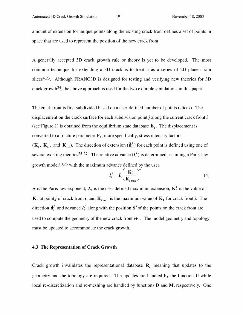
Assume that an internal elliptical crack, defined by the shaded area in Figure 13, has been
analyzed and the new crack front points determined as described in Section 4.2. The
propagation of this crack is described next.
Figure 13. An internal elliptical crack is defined by the shaded area.
The set of points (+ symbols) define the predicted new crack front.
4.3.1 Adding The New Crack Front Edges
A polynomial function is fit through the new crack front points. The function can be a single
n-th order polynomial, a continuous piecewise set of n-th order polynomials, or a set of cubic
Hermitian polynomials. The first two are used for surface cracks and the latter is used
exclusively for closed-loop crack fronts such as an internal crack front. A least-squares
routine is used to give the best function in all cases. From the function, a set of fitted points
is determined. The function serves two purposes: 1) it smoothes numerical and geometrical
distortions; and 2) it provides a convenient method for intersecting the crack front with the
Automated 3D Crack Growth Simulation 21 November 18, 2003
model surfaces.
The second step is to determine the region(s) in which the fitted points fall; they might lie
outside the model boundary. A simple ray casting technique28, extending the point-in-
polygon routine17 to 3D, is used for this purpose.
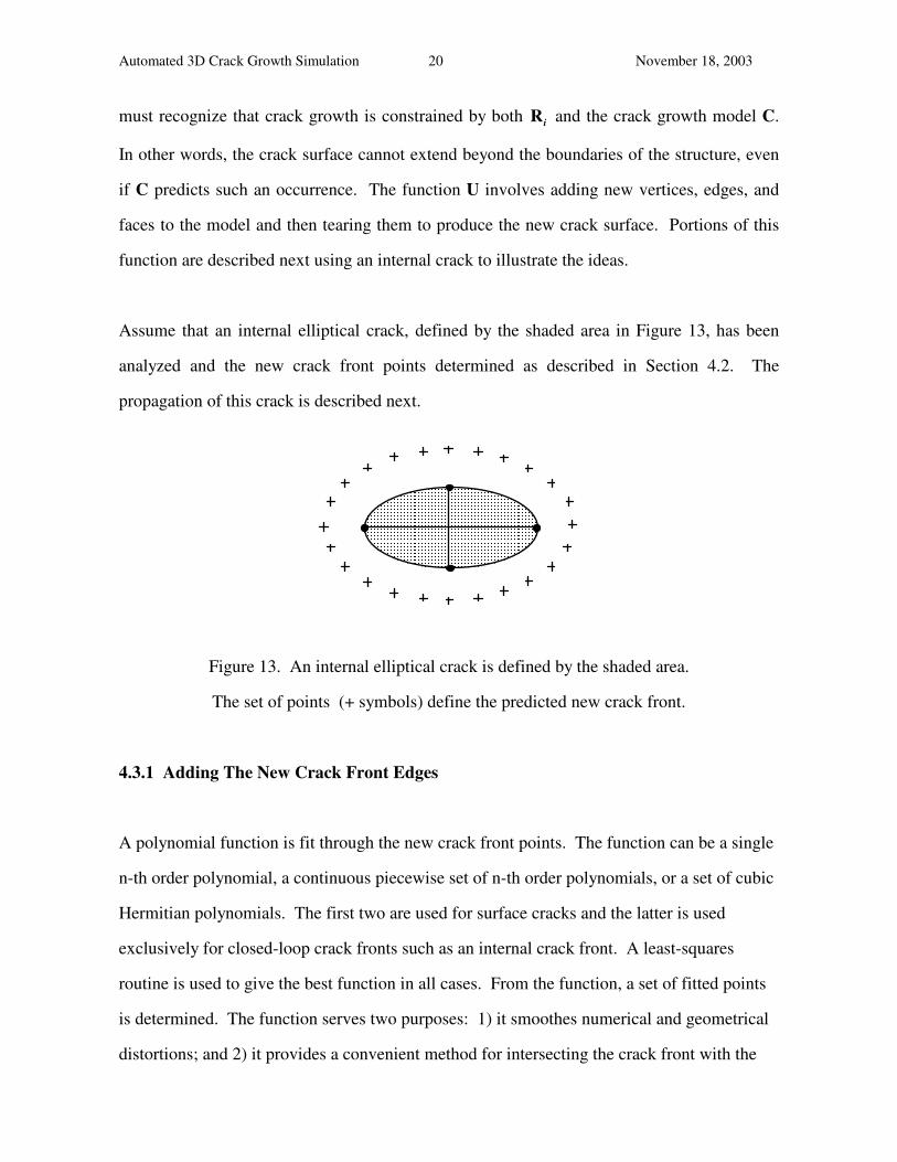
Finally, new edges are added to the model using the fitted points to define the edge geometry.
If the new front points fall in the same region as the original crack, adding the new edges is
straightforward. If the points fall in different regions, then edges will intersect surfaces and
the polynomial functions described above are used to find the intersection points.
Figure 14. New crack front edges added to the model through the fitted points.
The solid squares represent the vertices on the new crack front edges.
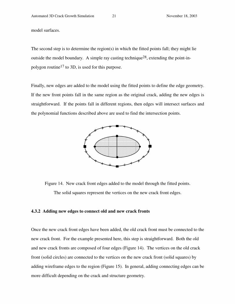
4.3.2 Adding new edges to connect old and new crack fronts
Once the new crack front edges have been added, the old crack front must be connected to the
new crack front. For the example presented here, this step is straightforward. Both the old
and new crack fronts are composed of four edges (Figure 14). The vertices on the old crack
front (solid circles) are connected to the vertices on the new crack front (solid squares) by
adding wireframe edges to the region (Figure 15). In general, adding connecting edges can be
more difficult depending on the crack and structure geometry.
Automated 3D Crack Growth Simulation 22 November 18, 2003
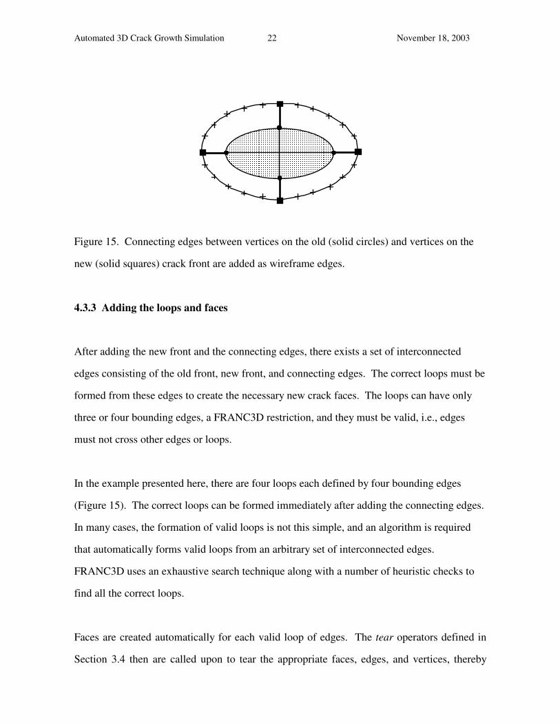
Figure 15. Connecting edges between vertices on the old (solid circles) and vertices on the
new (solid squares) crack front are added as wireframe edges.
4.3.3 Adding the loops and faces
After adding the new front and the connecting edges, there exists a set of interconnected
edges consisting of the old front, new front, and connecting edges. The correct loops must be
formed from these edges to create the necessary new crack faces. The loops can have only
three or four bounding edges, a FRANC3D restriction, and they must be valid, i.e., edges
must not cross other edges or loops.
In the example presented here, there are four loops each defined by four bounding edges
(Figure 15). The correct loops can be formed immediately after adding the connecting edges.
In many cases, the formation of valid loops is not this simple, and an algorithm is required
that automatically forms valid loops from an arbitrary set of interconnected edges.
FRANC3D uses an exhaustive search technique along with a number of heuristic checks to
find all the correct loops.
Faces are created automatically for each valid loop of edges. The tear operators defined in
Section 3.4 then are called upon to tear the appropriate faces, edges, and vertices, thereby
Automated 3D Crack Growth Simulation 23 November 18, 2003
propagating the crack.
4.4 Automation
Crack growth as described above consists of two parts: mechanics and representation.
Current crack growth mechanics are based on 2D theories and need to be replaced by an
acceptable 3D theory. The representation, which consists of the topology and geometry and
the associated functions and databases, is completely generic, however; any crack in any 3D
structure can be represented and propagated. In addition, crack propagation is completely
automated in FRANC3D; the user is not required to interact or intervene at any stage after
defining the initial cracked model.
The automated simulations rely on suitable numerical discretization techniques and accurate
analysis codes. FRANC3D supports both finite and boundary elements, but could be
modified to work with other numerical techniques29. Regardless of the numerical technique,
the discretization of the cracked structure must be accomplished such that the evolution of the
fracture is modeled accurately both in terms of numerics and geometry. In addition, the
discretization must be automatic, fast, and robust.
5. DISCRETIZATION AND MESHING
Crack growth simulations cause the geometry and, therefore, the mesh to continually change
as the crack evolves. To limit the time and effort spent on meshing and re-meshing, a
discretization function was designed to minimize the changes due to crack growth. This
function D uses a hierarchy of discretized models and also incorporates an automatic meshing
algorithm for meshing local portions of the model that are affected by crack growth.
Automated 3D Crack Growth Simulation 24 November 18, 2003
5.1 A Hierarchy of Models and Constraints
Thus far, only two independent representations of a structure, the geometry and mesh models
were mentioned. Actually, a hierarchy of five models is used in FRANC3D. Within the
model hierarchy is a strong notion of constraint. That is, entities at any level of the hierarchy
are constrained by those in the levels above it.
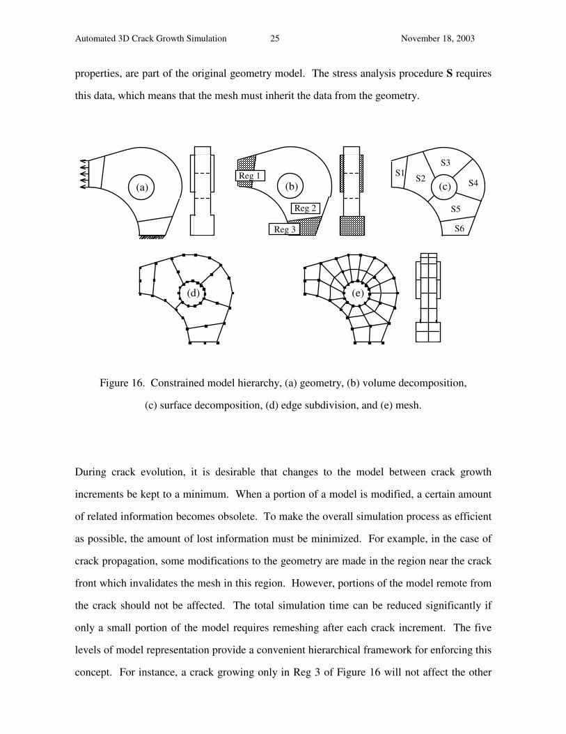
The geometry (Figure 16a) and mesh (Figure 16e) descriptions represent the highest and
lowest levels in the five-level hierarchy, respectively. The second highest level is a volume
decomposition level (Figure 16b) where regions of the geometric model can be divided into
subregions. This level is useful for defining regularly shaped regions for the volume meshing
algorithm. The third highest level is a surface decomposition level (Figure 16c). This level
is useful when decomposing an irregularly shaped surface into subsurfaces for surface
meshing purposes. The next level is the edge subdivision level (Figure 16d). This level has
two purposes. The spline space-curves of the three higher levels are approximated by
straight-line segments, and the subdivision edge size defines a metric for the local mesh
density. The lowest level in the hierarchy is the mesh, whether it’s a surface or volume mesh,
or a combination. All levels are constrained by the levels above, meaning that the lowest
mesh level has element edges that correspond to the edge subdivision level edges, element
faces cannot span surface subdivision boundaries, element volumes cannot span region
subdivision boundaries, and the entire mesh is constrained by the original geometry.
There are two primary purposes for such a hierarchy. One is to provide constraints and
inheritance for interactive modeling, and the other is to aid in minimizing changes to the
model during crack evolution.
The hierarchy allows the mesh level model to inherit the geometry and the simulation
attributes. Simulation attributes, which consist of boundary conditions and material
Automated 3D Crack Growth Simulation 25 November 18, 2003
properties, are part of the original geometry model. The stress analysis procedure S requires
this data, which means that the mesh must inherit the data from the geometry.
(b)(a)Reg 1
Reg 2
Reg 3
(c)
S5
S4
S3
S2S1
S6
(d) (e)
Figure 16. Constrained model hierarchy, (a) geometry, (b) volume decomposition,
(c) surface decomposition, (d) edge subdivision, and (e) mesh.
During crack evolution, it is desirable that changes to the model between crack growth
increments be kept to a minimum. When a portion of a model is modified, a certain amount
of related information becomes obsolete. To make the overall simulation process as efficient
as possible, the amount of lost information must be minimized. For example, in the case of
crack propagation, some modifications to the geometry are made in the region near the crack
front which invalidates the mesh in this region. However, portions of the model remote from
the crack should not be affected. The total simulation time can be reduced significantly if
only a small portion of the model requires remeshing after each crack increment. The five
levels of model representation provide a convenient hierarchical framework for enforcing this
concept. For instance, a crack growing only in Reg 3 of Figure 16 will not affect the other
Automated 3D Crack Growth Simulation 26 November 18, 2003
two regions, meaning that these two regions do not have to be re-discretized after every step
of propagation.
5.2 Meshing During Crack Growth Simulations
The purpose of the discretization function D is to transform a geometry database to an
analysis database that meets the input requirements of a particular stress analysis procedure.
The major portion of this task is the creation of a surface or volume mesh. An automatic
mesh generation capability can be employed. These are well described in the literature30-35.
There are two aspects of mesh generation that are important in the context of crack growth
simulation that may be less important in other applications. The first arises due to the
geometric coincidence of crack faces. A meshing algorithm used to mesh a surface or
volume containing crack faces, where the crack faces are represented by two distinct surfaces,
cannot rely on geometrical checks exclusively while generating elements. This is because
nodal points on opposing crack faces are distinct, but share a common location. It cannot be
determined from geometrical checks alone if a candidate node is on the proper side of a
crack. To properly mesh such regions, algorithms must resort to topological information to
select the proper node.
The second aspect of mesh generation is important when trying to minimize the changes to
the model during crack evolution. Often only a small portion of the body near the crack front
needs remeshing. However, the new mesh must conform to the remaining unchanged
portions of the mesh, which imposes additional constraints on the meshing algorithm. The
surface meshing algorithm implemented in FRANC3D was described by Potyondy et al. 34 .
A tetrahedral volume meshing algorithm using similar ideas has been implemented as well36.
FRANC3D maintains a consistent geometric representation of the model at each step of
Automated 3D Crack Growth Simulation 27 November 18, 2003
propagation. During fracture propagation, the previous crack surface geometry remains the
same; new fracture surface is simply added to the model to represent the crack growth.
Therefore, the mesh that is attached to the existing geometric crack surfaces is unaffected by
fracture growth because the existing geometry does not change. Actually, the mesh is
removed from the geometric crack surface during propagation, but an identical mesh can be
regenerated on that surface. A new mesh is attached to the new crack surface. The re-
discretization process has been automated completely so that crack growth simulations can
proceed from an initial cracked model without any user intervention.
6. ANALYSIS DATABASES
The stress analysis function S can be any numerical analysis procedure that takes in the
analysis database Ai and produces the equilibrium state information E i and the required
fracture parameters F i . The main requirement of the numerical method is the accurate
calculation of the displacements and stresses near the crack front. Both finite and boundary
element procedures have been developed for this purpose. For the example simulations
below, BES, a 3D linear elastic boundary element code37 is used, which means that only
surface meshing is required.
7. CRACK GROWTH SIMULATIONS
The ability of the above model to simulate crack propagation in 3D is best shown by practical
example. The purpose of this paper is to show that automated simulation of the complete 3D
crack growth evolution in a real-life engineered structure is possible with the appropriate
tools. Accordingly, two simulations are presented: one shows a simple geometry with a non-
planar crack surface, and the other shows a complex geometric structure with a planar crack
surface. In both cases, the crack transitions from a simple half-penny or quarter-penny
Automated 3D Crack Growth Simulation 28 November 18, 2003
shaped surface flaw to a part-through crack. For both examples, the stress intensity factor
history and fatigue life are presented and compared to experimental results after a number of
crack growth increments have been analyzed.
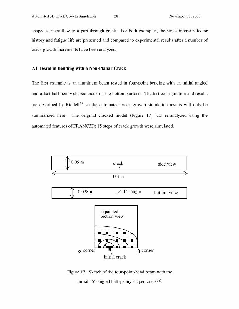
7.1 Beam in Bending with a Non-Planar Crack
The first example is an aluminum beam tested in four-point bending with an initial angled
and offset half-penny shaped crack on the bottom surface. The test configuration and results
are described by Riddell38 so the automated crack growth simulation results will only be
summarized here. The original cracked model (Figure 17) was re-analyzed using the
automated features of FRANC3D; 15 steps of crack growth were simulated.
0.3 m
side view0.05 m
bottom view45° angle0.038 m
αααα ββββ
expandedsection view
initial crackcornercorner
crack
Figure 17. Sketch of the four-point-bend beam with the
initial 45°-angled half-penny shaped crack38.
Automated 3D Crack Growth Simulation 29 November 18, 2003
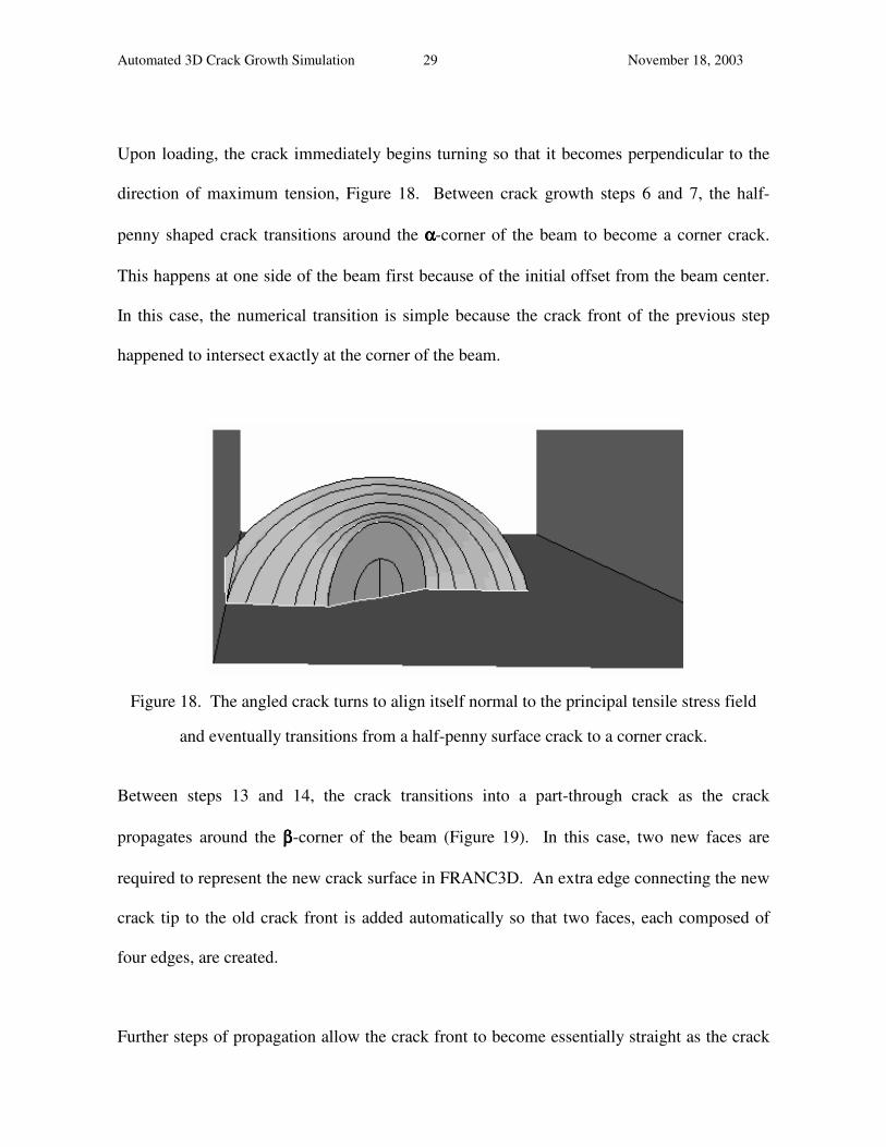
Upon loading, the crack immediately begins turning so that it becomes perpendicular to the
direction of maximum tension, Figure 18. Between crack growth steps 6 and 7, the half-
penny shaped crack transitions around the αααα-corner of the beam to become a corner crack.
This happens at one side of the beam first because of the initial offset from the beam center.
In this case, the numerical transition is simple because the crack front of the previous step
happened to intersect exactly at the corner of the beam.
Figure 18. The angled crack turns to align itself normal to the principal tensile stress field
and eventually transitions from a half-penny surface crack to a corner crack.
Between steps 13 and 14, the crack transitions into a part-through crack as the crack
propagates around the ββββ-corner of the beam (Figure 19). In this case, two new faces are
required to represent the new crack surface in FRANC3D. An extra edge connecting the new
crack tip to the old crack front is added automatically so that two faces, each composed of
four edges, are created.
Further steps of propagation allow the crack front to become essentially straight as the crack
Automated 3D Crack Growth Simulation 30 November 18, 2003
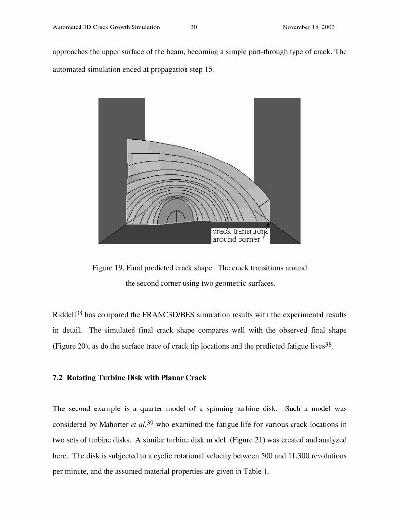
approaches the upper surface of the beam, becoming a simple part-through type of crack. The
automated simulation ended at propagation step 15.
Figure 19. Final predicted crack shape. The crack transitions around
the second corner using two geometric surfaces.
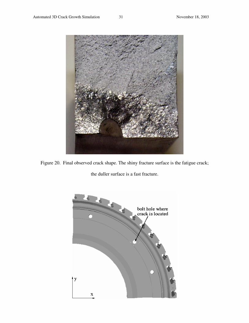
Riddell38 has compared the FRANC3D/BES simulation results with the experimental results
in detail. The simulated final crack shape compares well with the observed final shape
(Figure 20), as do the surface trace of crack tip locations and the predicted fatigue lives38.
7.2 Rotating Turbine Disk with Planar Crack
The second example is a quarter model of a spinning turbine disk. Such a model was
considered by Mahorter et al.39 who examined the fatigue life for various crack locations in
two sets of turbine disks. A similar turbine disk model (Figure 21) was created and analyzed
here. The disk is subjected to a cyclic rotational velocity between 500 and 11,300 revolutions
per minute, and the assumed material properties are given in Table 1.
Automated 3D Crack Growth Simulation 31 November 18, 2003
Figure 20. Final observed crack shape. The shiny fracture surface is the fatigue crack;
the duller surface is a fast fracture.
Automated 3D Crack Growth Simulation 32 November 18, 2003
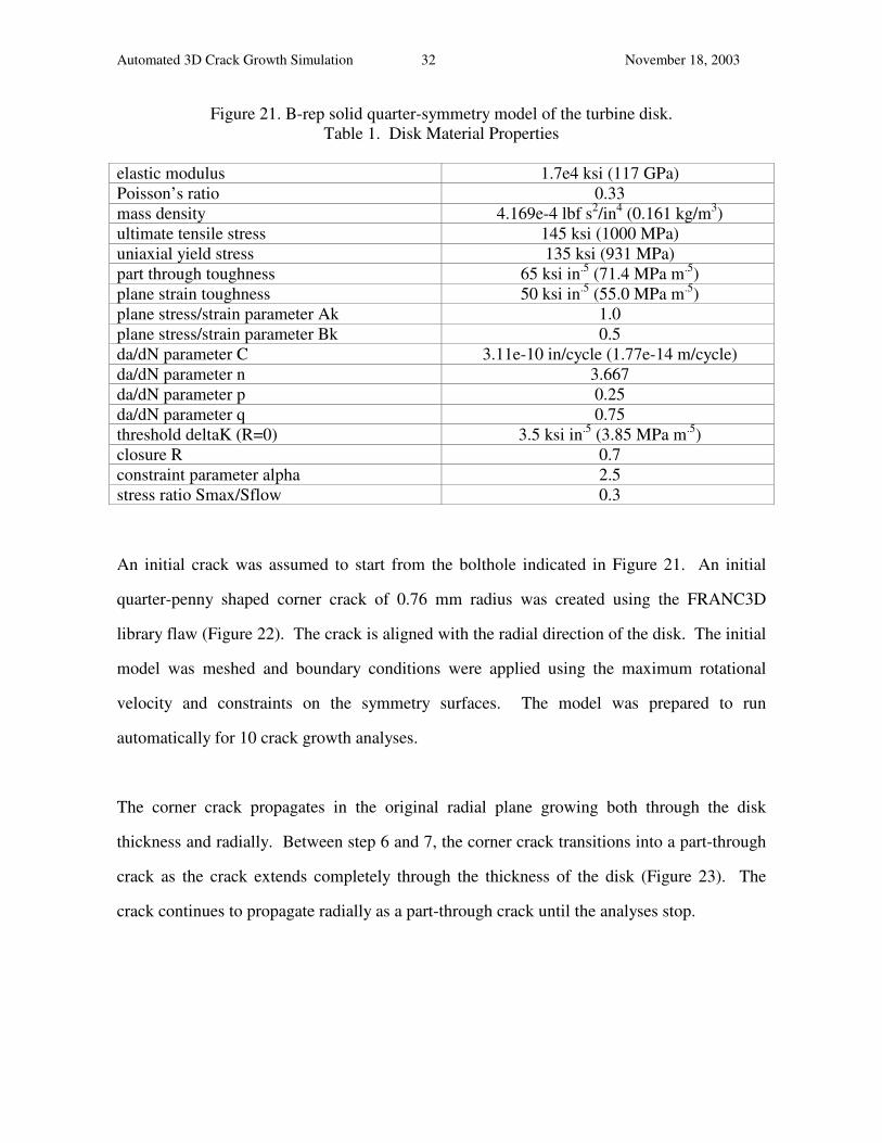
Figure 21. B-rep solid quarter-symmetry model of the turbine disk. Table 1. Disk Material Properties
elastic modulus 1.7e4 ksi (117 GPa) Poisson’s ratio 0.33 mass density 4.169e-4 lbf s2/in4 (0.161 kg/m3) ultimate tensile stress 145 ksi (1000 MPa) uniaxial yield stress 135 ksi (931 MPa) part through toughness 65 ksi in.5 (71.4 MPa m.5) plane strain toughness 50 ksi in.5 (55.0 MPa m.5) plane stress/strain parameter Ak 1.0 plane stress/strain parameter Bk 0.5 da/dN parameter C 3.11e-10 in/cycle (1.77e-14 m/cycle) da/dN parameter n 3.667 da/dN parameter p 0.25 da/dN parameter q 0.75 threshold deltaK (R=0) 3.5 ksi in.5 (3.85 MPa m.5) closure R 0.7 constraint parameter alpha 2.5 stress ratio Smax/Sflow 0.3
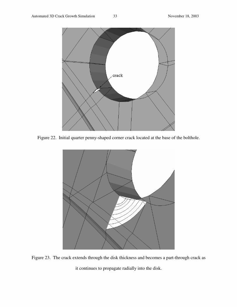
An initial crack was assumed to start from the bolthole indicated in Figure 21. An initial
quarter-penny shaped corner crack of 0.76 mm radius was created using the FRANC3D
library flaw (Figure 22). The crack is aligned with the radial direction of the disk. The initial
model was meshed and boundary conditions were applied using the maximum rotational
velocity and constraints on the symmetry surfaces. The model was prepared to run
automatically for 10 crack growth analyses.
The corner crack propagates in the original radial plane growing both through the disk
thickness and radially. Between step 6 and 7, the corner crack transitions into a part-through
crack as the crack extends completely through the thickness of the disk (Figure 23). The
crack continues to propagate radially as a part-through crack until the analyses stop.
Automated 3D Crack Growth Simulation 33 November 18, 2003
Figure 22. Initial quarter penny-shaped corner crack located at the base of the bolthole.
Figure 23. The crack extends through the disk thickness and becomes a part-through crack as
it continues to propagate radially into the disk.
Automated 3D Crack Growth Simulation 34 November 18, 2003
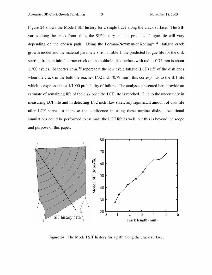
Figure 24 shows the Mode I SIF history for a single trace along the crack surface. The SIF
varies along the crack front; thus, the SIF history and the predicted fatigue life will vary
depending on the chosen path. Using the Forman-Newman-deKoning40,41 fatigue crack
growth model and the material parameters from Table 1, the predicted fatigue life for the disk
starting from an initial corner crack on the bolthole-disk surface with radius 0.76 mm is about
1,300 cycles. Mahorter et al.39 report that the low cycle fatigue (LCF) life of the disk ends
when the crack in the bolthole reaches 1/32 inch (0.79 mm); this corresponds to the B.1 life
which is expressed as a 1/1000 probability of failure. The analyses presented here provide an
estimate of remaining life of the disk once the LCF life is reached. Due to the uncertainty in
measuring LCF life and in detecting 1/32 inch flaw sizes, any significant amount of disk life
after LCF serves to increase the confidence in using these turbine disks. Additional
simulations could be performed to estimate the LCF life as well, but this is beyond the scope
and purpose of this paper.
0 1 2 3 4 5 620
30
40
50
60
70
80
crack length (mm)
Mod
e I S
IF (M
pa m
)
Figure 24. The Mode I SIF history for a path along the crack surface.
Automated 3D Crack Growth Simulation 35 November 18, 2003
.
0 200 400 600 800 1000 1200 14000
1
2
3
4
5
6
0 200 400 600 800 1000 1200 14000
1
2
3
4
5
6
number of cycles
crac
k le
ngth
(mm
)
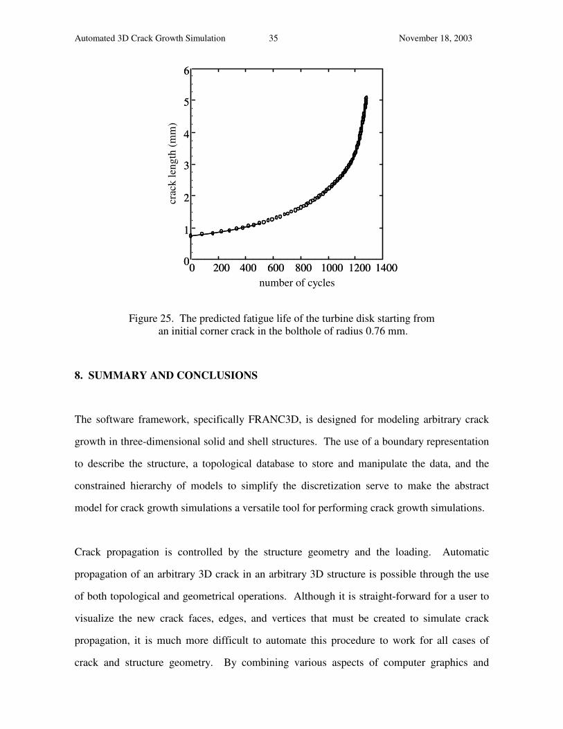
Figure 25. The predicted fatigue life of the turbine disk starting from
an initial corner crack in the bolthole of radius 0.76 mm.
8. SUMMARY AND CONCLUSIONS
The software framework, specifically FRANC3D, is designed for modeling arbitrary crack
growth in three-dimensional solid and shell structures. The use of a boundary representation
to describe the structure, a topological database to store and manipulate the data, and the
constrained hierarchy of models to simplify the discretization serve to make the abstract
model for crack growth simulations a versatile tool for performing crack growth simulations.
Crack propagation is controlled by the structure geometry and the loading. Automatic
propagation of an arbitrary 3D crack in an arbitrary 3D structure is possible through the use
of both topological and geometrical operations. Although it is straight-forward for a user to
visualize the new crack faces, edges, and vertices that must be created to simulate crack
propagation, it is much more difficult to automate this procedure to work for all cases of
crack and structure geometry. By combining various aspects of computer graphics and
Automated 3D Crack Growth Simulation 36 November 18, 2003
intelligent computational algorithms with some heuristic and logical checks, one can create a
system that is capable of handling very complex fracture propagation in a generic sense. Of
course, one needs a sophisticated topological database, such as the radial-edge database,
along with all the necessary Euler operators to represent, query, and efficiently manipulate
the model data.
All of the apparently tedious and time-consuming tasks: propagation, re-meshing, and re-
applying boundary conditions can be completely automated. The entire evolution of crack
growth can be simulated providing histories of stress intensity factors and predicted crack
shapes from which one can compute fatigue life. The software framework easily allows other
physical models for 3D crack growth to be implemented and tested, and new theories can
readily be compared to experimental or field studies by modeling the true structure and crack
geometry rather than an overly simplified or idealized model.
ACKNOWLEDGMENTS
Funding for the creation of FRANC3D has been provided in part by NASA (NAG-1-1184),
NSF (PYI 8351914), Boeing Commercial Airplane Group, Alcoa Foundation, Northrop
Grumman, and Schlumberger. The authors acknowledge the significant contributions of the
present and former members of the Cornell Fracture Group (CFG) in developing this
software and the concepts behind it. The software and documentation are freely available
from the CFG at http://www.cfg.cornell.edu.
REFERENCES
1. M. Ortiz 'Computational micromechanics', Comp. Mech., 18, 321-338 (1996).
Automated 3D Crack Growth Simulation 37 November 18, 2003
2. D.O. Potyondy, P.A. Wawrzynek, and A.R. Ingraffea, 'Discrete crack growth analysis
methodology for through cracks in pressurized fuselage structures', Int. J. Num. Meth.
Engng., 38, 1611-1633 (1995).
3. H.N. Linsbauer, A.R. Ingraffea, H.P. Rossmanith, and P.A. Wawrzynek, 'Simulation of
cracking in large arch dam', Part II, J. Struct. Engng., 115, 1616-1630 (1989).
4. P. Krysl, and T. Belytschko, 'Application of the element free Galerkin method to the
propagation of arbitrary 3D cracks', submitted to Int. J. Num. Meth. Engng. (1997).
5. R. Galdos, 'Finite element technique to simulate the stable shape evolution of planar
cracks with an application to semi-elliptical surface crack in a bimaterial finite solid', Int.
J. Num. Meth. Engng., 40, 905-917 (1997)
6. J. Cervenka, and V.E. Saouma, 'Numerical evaluation of 3-D SIF for arbitrary finite
element meshes', Engng. Fract. Mech., 57, 541-563 (1997).
7. P.E. O'Donoghue, S.N. Atluri, and D.S. Pipkins, 'Computational strategies for fatigue
crack growth in three dimensions with application to aircraft components', Engng. Fract.
Mech., 52, 51-64 (1995).
8. Y. Mi, and M.H. Aliabadi, 'Three-dimensional crack growth simulation using BEM',
Computers and Structures, 52, 871-878 (1994).
9. L.F. Martha, P.A. Wawrzynek, and A.R. Ingraffea, 'Arbitrary crack representation using
solid modeling', Engng. with Comp., 9, 63-82 (1993).
10. M.D. Gilchrist, and R.A. Smith, 'Finite element modelling of fatigue crack shapes',
Fatigue Fract. Engng. Mater. Struct., 14, 617-626 (1991).
11. I.S. Raju, and J.C. Newman, 'Three-dimensional finite element analysis of finite-
thickness fracture specimens', NASA TN D-8414 (1977).
12. L.F. Martha, A Topological and Geometrical Modeling Approach to Numerical
Discretization and Arbitrary Fracture Simulation in Three-Dimensions, Ph.D.
Dissertation, Cornell University, 1989.
13. P.A. Wawrzynek, Discrete Modeling of Crack Propagation: Theoretical Aspects and
Implementation Issues in Two and Three Dimensions, Ph.D. Dissertation, Cornell
Automated 3D Crack Growth Simulation 38 November 18, 2003
University, 1991.
14. D.O Potyondy, A software framework for simulating curvilinear crack growth in
pressurized thin shells, Ph.D. Dissertation, Cornell University, 1993.
15. C.M. Hoffmann, Geometric and Solid Modeling: An Introduction, Morgan Kaufmann
Publishers, Inc., San Mateo, California, 1989.
16. M. Mäntylä, An Introduction to Solid Modeling, Computer Science Press, Rockville,
Maryland, 1988.
17. M.E. Mortenson, Geometric Modeling, 2nd edn, John Wiley & Sons, New York, 1997.
18. K. Weiler, Topological Structures for Geometric Modeling, Ph.D. Dissertation,
Rensselaer Polytechnic Institute, Troy, NY, 1986.
19. P.A. Wawrzynek, and A.R. Ingraffea, 'Interactive finite element analysis of fracture
processes: an integrated approach', Theor. & Appl. Fract. Mech., 8, 137-150 (1987).
20. P.A. Wawrzynek, and A.R. Ingraffea, 'An edge-based data structure for two-dimensional
finite element analysis', Engng. with Comp., 3, 13-20 (1987).
21. B.G. Baumgart, 'A polyhedron representation for computer vision', AFIPS Proc., 44,
589-596 (1975).
22. K. Weiler, 'Edge-based data structures for solid modeling in curved-surface
environments', IEEE Comp. Graph. & Appl., 5, 21-40 (1985).
23. J.L. Sousa, L.F. Martha, P.A. Wawrzynek and A.R. Ingraffea, 'Simulation of non-planar
crack propagation in three-dimensional structures in rock and concrete', in Fracture of
Rock and Concrete: Recent Developments, Shah, Swartz and Barr Editors, Elsevier
Applied Science, London, 254-264 (1989).
24. R. Singh, B.J. Carter, P.A. Wawrzynek, and A.R. Ingraffea, 'Universal crack closure
integral for SIF estimation', Engng. Fract. Mech., 60, 133-146 (1998).
25. F. Erdogan and G.C. Sih, 'On the crack extension of plates under plane loading and
transverse shear. J. Basic Engng., 85, 519-527 (1963).
26. M.A. Hussain, S.U. Pu, and J. Underwood, 'Strain energy release rate for a crack under
combined Mode I and II', ASTM STP 560, 2-28 (1974).
Automated 3D Crack Growth Simulation 39 November 18, 2003
27. G.C. Sih, 'Strain-energy-density factor applied to mixed-mode crack problems', Int. J.
Fract. Mech., 10, 305-321 (1974).
28. S.D. Roth, 'Ray casting for modeling solids', Computer Graphics and Image Processing,
18, 109-144 (1982).
29. T. Belytschko, Y. Krongauz, D. Organ, M. Fleming, and P. Krysl, 'Meshless methods:
An overview and recent developments', Comp. Meth. Appl. Mech. Engng., 139, 3-47
(1996).
30. P. Baehmann, S. Wittchen, M.S. Shephard, 'Robust geometrically based, automatic two-
dimensional mesh generation', Int. J. Num. Meth. Engng., 24, 1043-1078 (1987).
31. J.C. Cavendish, D.A. Field, and W.H. Frey, 'An approach to automatic three-
dimensional finite element mesh generation', Int. J. Num. Meth. Engng., 21, 329-347
(1985).
32. A. Kela, M. Saxena, and R. Perucchio, 'A hierarchical structure for automatic meshing
and adaptive FEM analysis', Engng. Comput., 4, 104-112 (1987).
33. S.H. Lo, 'Delaunay triangulation of non-convex planar domains,' Int. J. Num. Meth.
Engng., 28, 2695-2707 (1989).
34. D.O. Potyondy, P.A. Wawrzynek, and A.R. Ingraffea, 'An algorithm to generate
quadrilateral or triangular element surface meshes in arbitrary domains with applications
to crack propagation', Int. J. Num. Meth. in Engng., 38, 2677-2701 (1995).
35. M.S. Shephard, 'Finite element modeling within an integrated geometric modeling
environment: Parts I and II, Engng. Comput., 1, 61-71 (1985).
36. J. Cavalcante, (1997) Personal communication.
37. E.D. Lutz, Numerical Methods for Hypersingular and Near-Singular Boundary
Integrals in Fracture Mechanics, Ph.D. Dissertation, Cornell University, 1991.
38. W.T. Riddell, A.R. Ingraffea, and P.A. Wawrzynek, 'Experimental observations and
numerical prediction of non-planar fatigue crack propagation, Engng. Fract. Mech., 58,
293-310 (1997).
39. R. Mahorter, G. London, S. Fowler and J. Salvino, 'Life prediction methodology for
Automated 3D Crack Growth Simulation 40 November 18, 2003
aircraft gas turbine engine disks', AIAA/SAE/ASME/ASEE 21st Joint Propulsion
Conference, Monterey, CA, 1-6 (1985).
40. R.G. Forman, V. Shivakumar, J.C. Newman, 'Fatigue crack growth computer program
"NASA/FLAGRO" Version 2.0', Johnson Space Center, Houston, Texas, Rpt. #JSC-
22267A (1994).
41. R.G. Forman, S.R. Mettu, 'Behavior of surface and corner cracks subjected to tensile and
bending loads in Ti-6Al-4V alloy', Fracture Mechanics: Twenty-second Symposium, 1,
ASTM STP 1131, Ernst, Saxena, & McDowell, eds., American Society for Testing and
Materials, Philadelphia, 519-546 (1992).