Embed Size (px)
Citation preview
Autoionizing states and their relevance in electron-ion
recombination
Dragan Nikolić
AKADEMISK AVHANDLING
Som med tillstånd av Stockholms Universitet
framlägges till offentlig granskning för avläggande av
filosofie doktorsexamen fredagen den 04 Juni 2004, kl 13.00 i föreläsningssalen FB42
Alba Nova, Roslagstullsbacken 21, Stockholm
Department of Physics Stockholm University
2004

Autoionizing states and their relevance in electron-ion recombination Dragan Nikolić ISBN 91-7265-906-8 pp 1-67 Stockholms universitet AlbaNova universitetscentrum Fysikum SE - 106 91 Stockholm SWEDEN Universitetsservice US-AB STOCKHOLM 2004

Violeti

Preface
This dissertation presents research I have carried out between November 2000
and March 2004 under the supervision of Prof. Eva Lindroth, in the Atomic Physics
group at Stockholm University.
My intention was to write as much a self-contained text as possible, which should
be understandable for a reader with a general knowledge of atomic physics, and
simultaneously contain most of the information the expert might be interested in.
This hopefully explains the size of this thesis, which has been organized as follows.
The first part consists of two chapters. Chapter 1 is an introduction to physical
phenomena treated in the included papers, especially electron-ion recombination.
The development and interpretation of storage-ring experiments, made on highly
charged ions, stimulated the appearance of theoretical methods capable of treating
many-body systems completely relativistically. Chapter 2 introduces the reader to
the basics of relativistic framework and QED corrections used in this thesis. The
ability to handle doubly (or multiply) excited autoionizing states is crucial for
calculations of electron-ion recombination. Although the conventional effective
Hamiltonian formalism (employing the coupled-cluster scheme) could be successfully
applied to many lithium-like ions, intruder states prevent its application in many cases.
The second part (Chapter 3) is dedicated to this intruder state problem. After a
brief review of the available methods for reduction of the full Hamiltonian, the
intruder state problem is addressed as the main obstacle for a global convergence of
the conventional set of pair equations. One particular remedy based on a suitable
partitioning of the full Hamiltonian is represented as a new contribution to the field.
Since the content of the thesis is shaped by a collection of attached articles, I plead
with the reader to have some understanding for any notation conflicts.
In the last part, Chapter 4 demonstrates the efficacy of newly developed
numerical implementation in dealing with the intruder state problem. As a test case,
several autoionizing doubly excited states in the helium atom, placed in the energy
region affected by the intruder state problem, are calculated within a non-relativistic
framework and compared to the results of other authors. In addition, our ability to
predict the recombination spectra of lithium like ions is elaborated within the
relativistic approach.

Articles attached to this thesis
I. Dielectronic recombination of lithiumlike beryllium: A theoretical and experimental investigation
by Tarek Ali Mohamed, Dragan Nikolić, Eva Lindroth, Stojan Madžunkov, Michael Fogle, Maria Tokman, and Reinhold Schuch, Physical Review A 66, 022719 (2002).
II. Dielectronic recombination resonances in Na8+ by Dragan Nikolić, Eva Lindroth, Stefan Kieslich, Carsten Brandau, Stefan Schippers, Wei Shi, Alfred Müller, Gerald Gwinner, Michael Schnell and Andreas Wolf, Submitted to Physical Review A (2004).
III. Intermediate Hamiltonian to avoid intruder state problems for doubly excited states
by Dragan Nikolić and Eva Lindroth, Submitted to Journal of Physics B (2004).
Articles not included in the thesis
IV. High resolution studies of electron-ion recombination
by Reinhold Schuch, Michael Fogle, Peter Glans, Eva Lindroth, Stojan Madzunkov, Tarek Mohamed and Dragan Nikolić, Radiation Physics and Chemistry 68, 51 (2003).
V. Determination of ion-broadening parameter for some Ar I spectral lines
by Dragan Nikolić, Stevica Đurović, Zoran Mijatović, Radomir Kobilarov, Bozidar Vujičić and Mihaela Ćirišan, Journal of Quantitative Spectroscopy and Radiative Transfer 86, 285 (2004).
VI. Comment on "Atomic spectral line-free parameter deconvolution procedure"
by Dragan Nikolić, Stevica Đurović, Zoran Mijatović and Radomir Kobilarov, Physical Review E 67, 058401 (2003).
VII. Asymmetry and Shifts Interdependence in Stark Profiles
by Alexander Demura, Volkmar Helbig and Dragan Nikolić, Spectral Line Shapes, AIP Conference Proceedings 645, 318 (2002)
VIII. Line shape study of neutral argon lines in plasma of an atmospheric pressure wall stabilized argon arc
by Stevica Đurović, Dragan Nikolić, Zoran Mijatović, Radomir Kobilarov and Nikola Konjević, Plasma Sources Science and Technology 11, IoP Publishing, A95 (2002)
IX. A simple method for bremsstrahlung spectra reconstruction from transmission measurements
by Miodrag Krmar, Dragan Nikolić, Predrag Krstonošić, Stefania Cora, Paolo Francescon, Paola Chiovati and Aleksandar Rudić, Medical Physics 29(6), 932 (2002).
X. Deconvolution of plasma broadened non-hydrogenic neutral atom lines
by Dragan Nikolić, Zoran Mijatović, Stevica Đurović, Radomir Kobilarov and Nikola Konjević, Journal of Quantitative Spectroscopy and Radiative Transfer 70, 67 (2001).

Table of Contents
Preface v Articles attached to this thesis vii Table of Contents ix List of Figures x List of Tables xi Chapter 1 Introduction 1
1.1 Relevant atomic processes in electron-ion recombination 3 1.2 Recombination of lithium-like ions 5 1.3 Recombination cross section 7
Chapter 2 Background Atomic Theory 11 2.1 The Dirac Hamiltonian 12 2.2 No-virtual-pair approximation 14 2.3 Breit interaction 15 2.4 Mass polarization 15 2.5 Radiative corrections 16
Chapter 3 Reduced Hamiltonians 19 3.1 Reduction by projection technique 20 3.2 Intruder state problem and intermediate Hamiltonians 25 3.3 State selective Hamiltonian 29
Chapter 4 Numerical implementations 39 4.1 Non-relativistic framework 39
4.1.1 One-electron spectrum 40 4.1.2 Two-electrons spectrum 42 4.1.3 Optimization of numerical calculations 43
4.2 Li-like and Be-like ions in a relativistic framework 50 4.2.1 Computational method 51 4.2.2 The lithium-like ions 55 4.2.3 The beryllium-like ions 56 4.2.4 Recombination cross section 57 4.2.5 Comparison with Storage-Ring experiments 59
Concluding Remarks 61 Acknowledgements 63 Bibliography 64
List of Figures
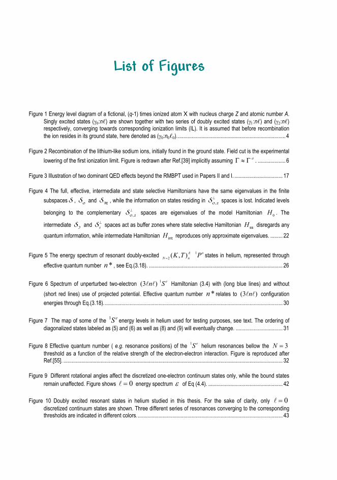
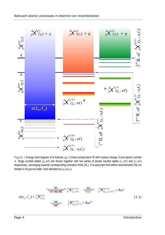
Figure 1 Energy level diagram of a fictional, (q-1) times ionized atom X with nucleus charge Z and atomic number A. Singly excited states (γ0:n) are shown together with two series of doubly excited states (γ1:n) and (γ2:n) respectively, converging towards corresponding ionization limits (IL). It is assumed that before recombination the ion resides in its ground state, here denoted as (γ0:n00)............................................................................... 4
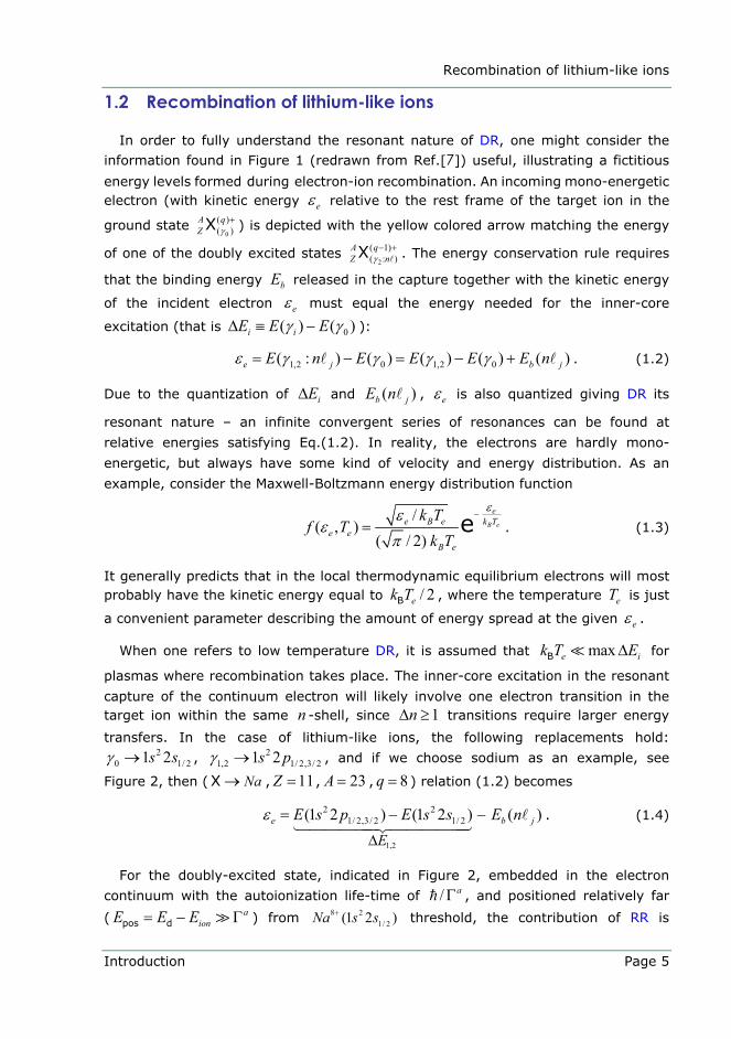
Figure 2 Recombination of the lithium-like sodium ions, initially found in the ground state. Field cut is the experimental lowering of the first ionization limit. Figure is redrawn after Ref.[39] implicitly assuming aΓ ≈ Γ . .................... 6
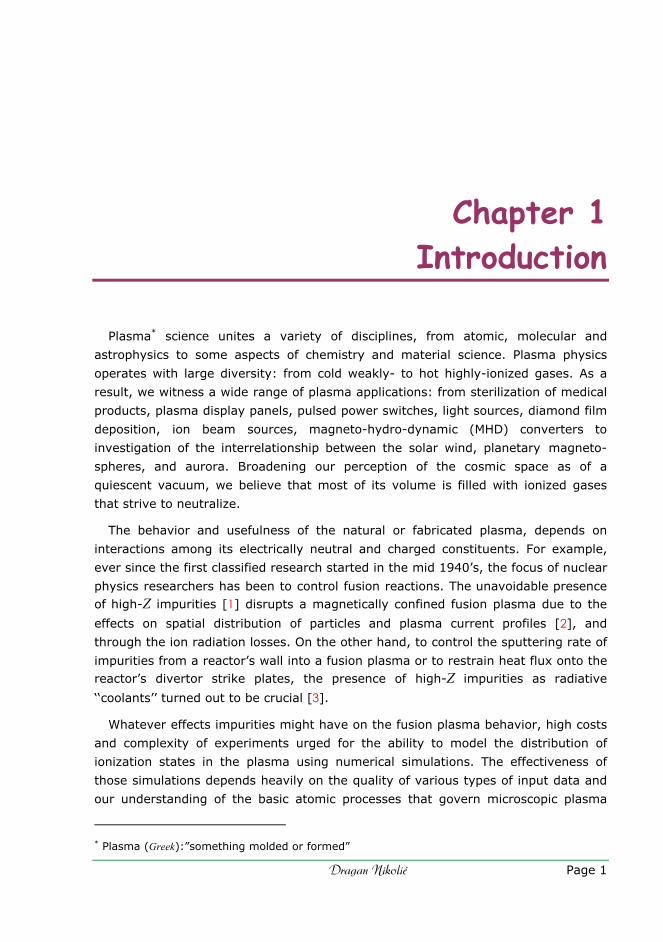
Figure 3 Illustration of two dominant QED effects beyond the RMBPT used in Papers II and I. ................................... 17
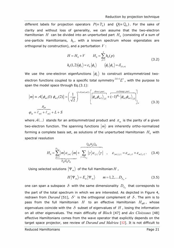
Figure 4 The full, effective, intermediate and state selective Hamiltonians have the same eigenvalues in the finite subspaces S , 0S and MS , while the information on states residing in ,
⊥0 2S spaces is lost. Indicated levels
belonging to the complementary ,⊥0 2S spaces are eigenvalues of the model Hamiltonian 0H . The
intermediate IS and ⊥1S spaces act as buffer zones where state selective Hamiltonian ssH disregards any
quantum information, while intermediate Hamiltonian intH reproduces only approximate eigenvalues. ......... 22
Figure 5 The energy spectrum of resonant doubly-excited 12 ( , )A o
N nK T P= states in helium, represented through effective quantum number *n , see Eq.(3.18). ................................................................................................. 26
Figure 6 Spectrum of unperturbed two-electron 1(3 ) en S Hamiltonian (3.4) with (long blue lines) and without (short red lines) use of projected potential. Effective quantum number *n relates to (3 )n configuration energies through Eq.(3.18).................................................................................................................................. 30
Figure 7 The map of some of the 1 eS energy levels in helium used for testing purposes, see text. The ordering of diagonalized states labeled as (5) and (6) as well as (8) and (9) will eventually change. .................................. 31
Figure 8 Effective quantum number ( e.g. resonance positions) of the 1 eS helium resonances bellow the 3N = threshold as a function of the relative strength of the electron-electron interaction. Figure is reproduced after Ref.[55]. ............................................................................................................................................................... 32
Figure 9 Different rotational angles affect the discretized one-electron continuum states only, while the bound states remain unaffected. Figure shows 0= energy spectrum ε of Eq (4.4). ...................................................... 42
Figure 10 Doubly excited resonant states in helium studied in this thesis. For the sake of clarity, only 0= discretized continuum states are shown. Three different series of resonances converging to the corresponding thresholds are indicated in different colors. ......................................................................................................... 43
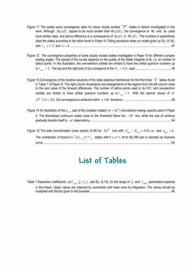
Figure 11 The partial wave convergence rates for seven doubly excited 1 oP states in helium investigated in this work. Although E∆Im appear to be much smaller than E∆Re , the convergence of Re and Im parts have similar rates, and above difference is a consequence of E EIm Re . The numbers in parenthesis label the states according to the table found in Paper III. Fitting procedure relies on model given by Eq. (4.16), with 0 1/ 2= and 4n = . ................................................................................................................................ 47
Figure 12 The convergence properties of some doubly excited states investigated in Paper III for different complex scaling angles. The spread of the curves depends on the quality of the Slater integrals (4.9), i.e. on number of lattice points. In this illustration, the one-electron orbitals are limited to have the orbital quantum numbers up to max 3= . The top and the right axis of (a) correspond to the 151pN = case. ............................................. 48
Figure 13 Convergence of the iterative solutions of the state selective Hamiltonian for the first three 1 eS states found in Table 1 of Paper III. The right column illustrations are enlargements of the regions from the left column close to the zero value of the forward differences. The number of lattice points used is Np=151, and one-electron orbitals are limited to have orbital quantum numbers up to max 3= . With the optimal choice of θ
0(5 24)θ≤ ≤ full convergence is achieved within 160≈ iterations. ............................................................. 49
Figure 14 An illustration of the 1/ 2s part of the complex rotated ( 010θ = ) one electron energy spectra used in Paper II. The discretized continuum states close to the threshold follow the 2θ− line, while the rest of continua gradually transfer itself to θ− dependency. ....................................................................................................... 54
Figure 15 The total recombination cross section (4.28) for 8Na + ions with 0.02ion cutE E au≈− and max 8n = .
The contribution of bound 21/ 2 "(1 )2 " " js s n states with 9 " 40n≤ ≤ to the RR part is denoted as Kramers
curve. ................................................................................................................................................................... 59
List of Tables
Table 1 Expansion coefficients max 0( , , )η ξ , see Eq. (4.16), for the range of ξ and max parameters explored in this thesis. Upper values are obtained by summation and lower ones by integration. The values should be multiplied with factors given in the brackets. ....................................................................................................... 46

Dragan Nikolié Page 1
Chapter 1 Introduction
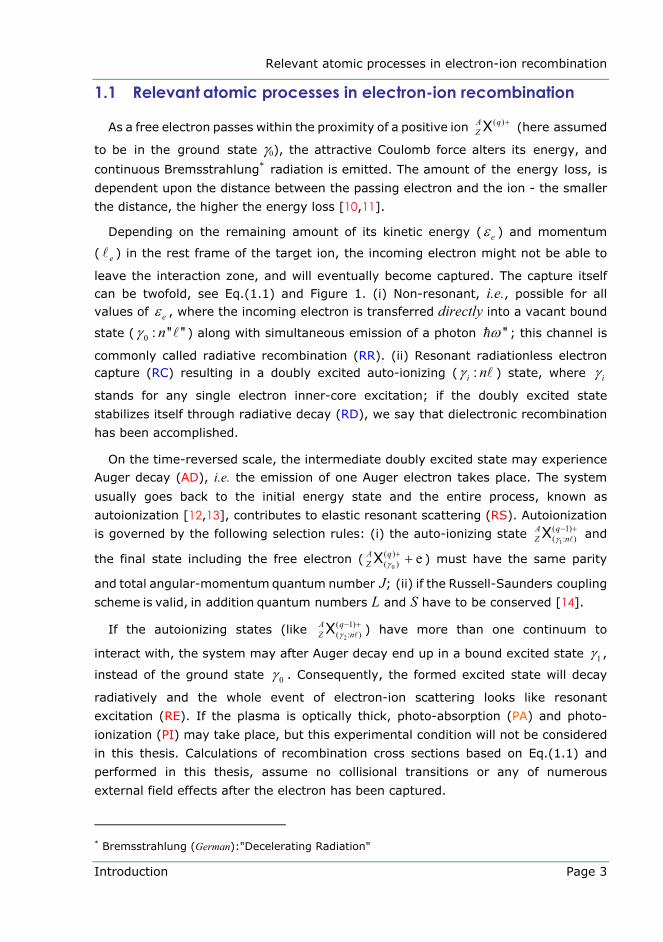
Plasma* science unites a variety of disciplines, from atomic, molecular and
astrophysics to some aspects of chemistry and material science. Plasma physics
operates with large diversity: from cold weakly- to hot highly-ionized gases. As a
result, we witness a wide range of plasma applications: from sterilization of medical
products, plasma display panels, pulsed power switches, light sources, diamond film
deposition, ion beam sources, magneto-hydro-dynamic (MHD) converters to
investigation of the interrelationship between the solar wind, planetary magneto-
spheres, and aurora. Broadening our perception of the cosmic space as of a
quiescent vacuum, we believe that most of its volume is filled with ionized gases
that strive to neutralize.
The behavior and usefulness of the natural or fabricated plasma, depends on
interactions among its electrically neutral and charged constituents. For example,
ever since the first classified research started in the mid 1940’s, the focus of nuclear
physics researchers has been to control fusion reactions. The unavoidable presence
of high-Z impurities [1] disrupts a magnetically confined fusion plasma due to the
effects on spatial distribution of particles and plasma current profiles [2], and
through the ion radiation losses. On the other hand, to control the sputtering rate of
impurities from a reactor’s wall into a fusion plasma or to restrain heat flux onto the reactor’s divertor strike plates, the presence of high-Z impurities as radiative
‘‘coolants’’ turned out to be crucial [3].
Whatever effects impurities might have on the fusion plasma behavior, high costs
and complexity of experiments urged for the ability to model the distribution of
ionization states in the plasma using numerical simulations. The effectiveness of
those simulations depends heavily on the quality of various types of input data and
our understanding of the basic atomic processes that govern microscopic plasma
* Plasma (Greek):”something molded or formed”

Relevant atomic processes in electron-ion recombination
Page 2 Introduction
properties. Among the most important are autoionization, collisional and radiative
ionization balanced by radiative decay and recombination processes, generally
taking place in non-equilibrium conditions such as those in low-density high-
temperature astrophysical and laboratory plasmas. The excitation processes
predominantly occur through collisions of ground-state ions with electrons having a
Maxwellian-like velocity distribution. Proper relevant plasma parameters (such as
electron number density and temperature distribution, abundances of neutrals and
ions) can be obtained only with the state-of-the-art calculations benchmarked with
reliable experiments.
Turning now more specifically to electron-ion recombination in low-density
plasmas, it is found that this important process dominantly occurs through two
coupled channels: directly via the electron continuum and via resonances embedded in it. Recombination through the non-resonant continuum is referred as radiative recombination (RR) and recombination involving the autoionizing resonances as
dielectronic recombination (DR). It is interesting, after six decades, to recall what
Massey and Bates [4] concluded in their first addressing of DR:
“In order that an electron should recombine with an O+ ion to reform an O atom in the normal or an excited state, the surplus energy of the electron must be got rid of in some way. If the pressure is so low that no third body is likely to be sufficiently close to receive the energy, only two modes of energy disposal are possible. Either it is directly radiated or else is communicated to a second electron in the O+ ion, raising it to an excited orbital. In the latter case, the state in which the incident and second electron are both in excited orbitals is not stable and can either revert to the initial condition by re-emission of an electron or, by emission of radiation, undergo a transition to a stable state of the neutral atom, leading thus to recombination. This process is the inverse of that known as auto-ionization, and its contribution cannot be ignored. Since it depends on interaction between two electrons we refer to it henceforward as dielectronic recombination.”
Since then, DR has been extensively studied and an excellent introduction and survey of early literature can be found in the review articles of Seaton and Storey [5]
and Bell and Seaton [6]. Extensive reviews dealing with applications of DR in
astrophysics have been contributed by Dubau and Volonté [7] and by Roszman [8].
It was customary in early theoretical models to separately analyze those two
recombination channels, and the first unified treatment of radiative and dielectronic recombination was reported by Alber et al [9].
In the remaining part of this introduction, a brief summary of possible outcomes
of an electron-ion collision is presented. Some widely adopted abbreviations will be
set and used in the rest of this thesis.
Relevant atomic processes in electron-ion recombination
Introduction Page 3
1.1 Relevant atomic processes in electron-ion recombination
As a free electron passes within the proximity of a positive ion ( )XA qZ
+ (here assumed
to be in the ground state γ0), the attractive Coulomb force alters its energy, and continuous Bremsstrahlung* radiation is emitted. The amount of the energy loss, is
dependent upon the distance between the passing electron and the ion - the smaller
the distance, the higher the energy loss [10,11].
Depending on the remaining amount of its kinetic energy ( eε ) and momentum
( e ) in the rest frame of the target ion, the incoming electron might not be able to
leave the interaction zone, and will eventually become captured. The capture itself can be twofold, see Eq.(1.1) and Figure 1. (i) Non-resonant, i.e., possible for all values of eε , where the incoming electron is transferred directly into a vacant bound
state ( 0 : '' ''nγ ) along with simultaneous emission of a photon ''ω ; this channel is
commonly called radiative recombination (RR). (ii) Resonant radiationless electron capture (RC) resulting in a doubly excited auto-ionizing ( :i nγ ) state, where iγ
stands for any single electron inner-core excitation; if the doubly excited state
stabilizes itself through radiative decay (RD), we say that dielectronic recombination
has been accomplished.
On the time-reversed scale, the intermediate doubly excited state may experience Auger decay (AD), i.e. the emission of one Auger electron takes place. The system
usually goes back to the initial energy state and the entire process, known as
autoionization [12,13], contributes to elastic resonant scattering (RS). Autoionization
is governed by the following selection rules: (i) the auto-ionizing state 1
( 1)( : )XA q
Z nγ− + and
the final state including the free electron (0
( )( ) eXA q
Z γ+ + ) must have the same parity
and total angular-momentum quantum number J; (ii) if the Russell-Saunders coupling
scheme is valid, in addition quantum numbers L and S have to be conserved [14].
If the autoionizing states (like 2
( 1)( : )XA q
Z nγ− + ) have more than one continuum to
interact with, the system may after Auger decay end up in a bound excited state 1γ ,
instead of the ground state 0γ . Consequently, the formed excited state will decay
radiatively and the whole event of electron-ion scattering looks like resonant
excitation (RE). If the plasma is optically thick, photo-absorption (PA) and photo-
ionization (PI) may take place, but this experimental condition will not be considered
in this thesis. Calculations of recombination cross sections based on Eq.(1.1) and
performed in this thesis, assume no collisional transitions or any of numerous
external field effects after the electron has been captured.
* Bremsstrahlung (German):"Decelerating Radiation"
Relevant atomic processes in electron-ion recombination
Page 4 Introduction
Figure 1 Energy level diagram of a fictional, (q-1) times ionized atom X with nucleus charge Z and atomic number A. Singly excited states (γ0:n) are shown together with two series of doubly excited states (γ1:n) and (γ2:n) respectively, converging towards corresponding ionization limits (IL). It is assumed that before recombination the ion resides in its ground state, here denoted as (γ0:n00).
0
0
0
( 1) ( 1)( : ) ( , : ' ')
( )( )
( 1)( : '' '')
'
e( , )''
AD: , X X
XX
i i
A q A qZ n Z n
A qe e Z
A qZ n
γ γ γ
γ
γ
ω
εω
− + − +
+
− +
+
++
P
RC RD
RR
ARS RE
PI
(1.1)
Recombination of lithium-like ions
Introduction Page 5
1.2 Recombination of lithium-like ions
In order to fully understand the resonant nature of DR, one might consider the
information found in Figure 1 (redrawn from Ref.[7]) useful, illustrating a fictitious
energy levels formed during electron-ion recombination. An incoming mono-energetic electron (with kinetic energy eε relative to the rest frame of the target ion in the
ground state 0
( )( )XA q
Z γ+ ) is depicted with the yellow colored arrow matching the energy
of one of the doubly excited states 2
( 1)( : )XA q
Z nγ− + . The energy conservation rule requires
that the binding energy bE released in the capture together with the kinetic energy
of the incident electron eε must equal the energy needed for the inner-core
excitation (that is 0( ) ( )i iE E Eγ γ∆ ≡ − ):
1,2 0 1,2 0( : ) ( ) ( ) ( ) ( )e j b jE n E E E E nε γ γ γ γ= − = − + . (1.2)
Due to the quantization of iE∆ and ( )b jE n , eε is also quantized giving DR its
resonant nature – an infinite convergent series of resonances can be found at
relative energies satisfying Eq.(1.2). In reality, the electrons are hardly mono-
energetic, but always have some kind of velocity and energy distribution. As an
example, consider the Maxwell-Boltzmann energy distribution function
/
( , )( / 2)
e B e
ee B e k T
e eB e
k Tf T
k T
εεε
π
−
= . (1.3)
It generally predicts that in the local thermodynamic equilibrium electrons will most probably have the kinetic energy equal to / 2B ek T , where the temperature eT is just
a convenient parameter describing the amount of energy spread at the given eε .
When one refers to low temperature DR, it is assumed that maxB e ik T E∆ for
plasmas where recombination takes place. The inner-core excitation in the resonant
capture of the continuum electron will likely involve one electron transition in the target ion within the same n -shell, since 1n∆ ≥ transitions require larger energy
transfers. In the case of lithium-like ions, the following replacements hold: 2
0 1/ 21 2s sγ → , 21,2 1/ 2,3/ 21 2s pγ → , and if we choose sodium as an example, see
Figure 2, then (X Na→ , 11Z = , 23A = , 8q = ) relation (1.2) becomes
1,2
2 21/ 2,3/ 2 1/ 2(1 2 ) (1 2 ) ( )e b j
E
E s p E s s E nε∆
= − − . (1.4)
For the doubly-excited state, indicated in Figure 2, embedded in the electron
continuum with the autoionization life-time of / aΓ , and positioned relatively far
( pos da
ionE E E= − Γ ) from 8 21/ 2(1 2 )Na s s+ threshold, the contribution of RR is

Recombination of lithium-like ions
Page 6 Introduction
negligible. The only recombination channel that is available to continuum electrons
is the DR path. If the doubly excited state has the radiative width rΓ , and do not
overlap with the other neighboring states of the same symmetry, its contribution to
the cross section for recombination to the arbitrary bound state sΨ , with the
energy sE , can be well characterized by a Lorentzian profile
2 2
/ 2( )( ) ( / 2)
dd
de
ion e
SE E
σ επ ε
Γ=
− − + Γ. (1.5)
Here a rΓ = Γ + Γ is the total width, while dS denotes the recombination strength for
the doubly excited state dΨ , with the energy dE , and represents the integrated
cross section
3 2
( )2 ( )
pos
dd d d d
0 d D ateR r
e e ione ion ion
E
gS d A Bm E E g
πσ ε ε →= = ⋅ ⋅−∫ RC . (1.6)
The initial ground state of the target 8 21/ 2(1 2 )Na s s+ ions has a multiplicity 2iong = ,
while the intermediate doubly excited state has multiplicity dg . The electron capture
rate dionA →RC may be equal to the auto-ionization rate aA , if dΨ can autoionize
only to the ground state of the target ion.
Figure 2 Recombination of the lithium-like sodium ions, initially found in the ground state. Field cut is the experimental lowering of the first ionization limit. Figure is redrawn after Ref.[39] implicitly assuming aΓ ≈ Γ .
Recombination cross section
Introduction Page 7
The probability for state dΨ to decay radiatively to an arbitrary bound state sΨ ,
is given by d srA → , and the branching ratio dB
d s
sd
d ss
r
a r
AB
A A
→
→
=+
∑∑
, (1.7)
which is the total probability of state dΨ to decay radiatively and complete the
process of DR. The radiative transition rate from the doubly excited dΨ to a
bound sΨ state, in the dipole approximation has the form
2 23
0
1 4 ( / )4 3
s s d d
d s
dsd s d
J M J Mr
M Mg
eA c rωπε→ = Ψ Ψ∑ . (1.8)
As (1.6) and (1.7) show, the strength strongly depends on the slowest type of
decay, which is in the case of light to medium heavy elements usually the radiative
decay (exceptions may occur for highly asymmetric doubly excited states).
For the doubly excited states positioned relatively close to the threshold
( posaE Γ∼ ), the contribution of RR is substantial. The Lorentzian description (1.5) of
the partial contribution to the cross section is strongly modified by the vicinity of
threshold, and the isolated resonance approach is not valid. Instead, RR and DR
should be treated in a unified manner, and one way of doing this is by using the
methods of photoionization calculations.
1.3 Recombination cross section
Our aim is to calculate the cross section for electron-ion recombination as a
function of relative collision energy. Since microscopic processes are symmetric
under time inversion, we can describe RR and DR in a unified way by using photo-
ionization method, often seen as an extension of photoabsorption approach. Rescigno and McKoy [15] used the method of complex scaling, to obtain the
photoabsorption cross section from a bound state sΨ :
( )2
0
1 4( ) /4 3
s s
s
ss
n n
n
i i
alln E E
r re cg
e eθ θ
ωπσ ω ω
πε→
Ψ Ψ Ψ Ψ
− −
⋅= ⋅ ∑PA Im . (1.9)
The partial photoabsorption cross section ( )s nσ ω→PA to each of the final states
nΨ , conducted with the photon energies ω capable of bringing the system
above the first ionization threshold ionE , can be used as an approximation for the
partial photo-ionization cross section ( )s nσ ω→PI . This is a valid approximation in the
Recombination cross section
Page 8 Introduction
cases studied here, since the autoionization rate aA dominates over the radiative
rate rA for almost all doubly excited states, see Papers II and I. This means that
the system, after photoabsorption, ends up in a doubly excited state above the
threshold, the decay of which is almost certainly by electron emission and will
eventually contribute to ionization. It is less likely that the doubly excited state
stabilizes itself radiatively, and even if it does so, the overall effect is negligible due
to the small strength. Thus the photoabsorption cross section (1.9) can be safely
used as the photoionization cross section, noting that the sum over the final states
nΨ includes all the optically allowed bound states, continuum states as well as
doubly excited states, with nE generally being complex. If the final state nΨ
represents the doubly excited state dΨ , see Figure 2 at page 6, the energy nE
equals / 2aion posE E i+ − Γ , and in addition the photon energy satisfies the relation
e sionE Eε ω+ = + . As in the case of Eq (1.8), the sum in Eq (1.9) runs over the all
magnetic sub-states ( nM and sM ), with the result averaged over the magnetic sub-
states of the initial state sΨ simply by division with its multiplicity sg . Using the
Milne relation [16] (i.e. the principle of detailed balance applied to the recombination
and photoionization)
2
0
/( ) ( )2
recomb ss sion e all
ion e e
g cg m
ωσ ε σ ωε→ →
⎛ ⎞= ⎜ ⎟⎜ ⎟
⎝ ⎠
PI (1.10)
and the energy conservation relation: e sionE Eε ω+ = + , one gets from (1.9)
( )32
0 0
/1 4( )4 3 2
recomb s ss
n nion
n ion e
i i
enion e e E E
r rceg m
e eθ θ
ε
ωπσ επε ε→
Ψ Ψ Ψ Ψ
− −
⋅= ⋅ ∑Im . (1.11)
The relation (1.11) takes into account the recombination through both of the
competitive channels, namely RR and DR, and may exhibit interference features of
these two channels in the case of recombination of lithium-like beryllium ions, see
Paper I.
In quantum mechanics, the existence of alternative pathways for a transition
between atomic states, gives rise to the phenomenon of interference: the
probability amplitudes, associated with each pathway, combine with a phase relationship. Beutler [17] reported the first experimental observation of this
phenomenon in photoabsorption spectra of noble gases. In that time considered an
anomaly in atomic spectroscopy, his spectra exhibited broad, highly asymmetric
absorption series. Beutler also proposed that this phenomenon is associated with autoionization, previously identified in atomic spectra by Majorana [12] and
Shenstone [13]. The same year, Fano [18] showed that spectral line profiles
observed by Beutler could be assigned to quantum mechanical interference in the

Recombination cross section
Introduction Page 9
autoionization, and presented a formula equivalent to his famous 1961 line shape profile, see Fano [19]. The development of sources of broadband synchrotron
radiation provided the far ultraviolet spectroscopy (5-150 nm), capable of observing
multiple electron excitations. The absorption spectra of helium was particularly
interesting, since the theory predicted two series of lines to be found, rather than the single one observed in the famous 1963 experiment of Madden and Codling
[20]. The same year, Cooper, Fano and Prats [21] showed that effects of electron
correlation tend to strongly favor the transitions to one of the two series. Soon
after, the two-electron dynamics became a prominent research subject in atomic
physics, and is still of interest today [22,23].

Dragan Nikolié Page 11
Chapter 2 Background Atomic Theory
The calculation of any atomic property requires the knowledge of the wave
functions of the relevant atomic states. According to quantum mechanics, see for example Messiah [24], a stationary state of an N - electron atom is described by a
wave function 1( , )Nq qΨ … , where the space and spin coordinates of the electron
labeled i , are represented by ( , )i i iq r σ≡ . The wave function is assumed continuous
over the space variables and is a solution to the wave equation
1( ) ( , ) 0NH E q q− Ψ =… , (2.1)
known as the time-independent form of Schrödinger’s equation. The solutions of the
eigenvalue problem (2.1) exist only for certain values of E , known as the eigen-
values of the Hamiltonian operator H , and represent the possible values of the
total energy of the atomic system. The operator H depends on the atomic system
and the employed quantum mechanical formalism. For non-relativistic calculations, H consists of the total kinetic energy of the N electrons plus the total potential
energy of the electrons due to their electrostatic interactions with the point charge
nucleus (usually assumed infinitively heavy) and with each other
( ) ( )0 0 0
2 1 1
1
2 212 4 4| | | |
N N
i i i ji i j
eZe e
mH p r r rπε πε− −
= <
= − + −∑ ∑ . (2.2)
It is possible to obtain exact solutions of (2.2) only for hydrogen-like ions, while the presence of the interelectronic distance | |ij i jr r r= − prevents the exact solvability of
Hamiltonian (2.2) already for two-electron systems. Therefore, two-electron ions are
one of the major systems of interest in development of methods that will yield
approximate but yet accurate wave functions.
The purpose of this Chapter is to introduce the basic results of Dirac’s relativistic
theory, since for accurate calculations of highly charged ions it is necessary to
discard the non-relativistic Hamiltonian (2.2). The relativistic, electron correlation
The Dirac Hamiltonian
Page 12 Background Atomic Theory
and quantum electrodynamics (QED) effects are thus only shortly discussed;
extensive approaches to this subject can be found in any relativistic quantum mechanics text book, see for example Greiner [25] and Thaller [26].
2.1 The Dirac Hamiltonian
The starting point of most relativistic quantum-mechanical methods is the Dirac
equation, which is the relativistic analog of the Schrödinger equation. Before Dirac’s
formulation, an obvious way of starting relativistic quantum mechanics would be the
relativistic energy-momentum relation
2 2 2 20( ) ( )eE m c pc= + (2.3)
and by inserting the appropriate quantum-mechanical operators for energy E and momentum p , the Klein-Gordon equation for a free electron will emerge
2 2 2 2
202 2 2 2 2( ) 0em c
c t x y zφ
⎛ ⎞∂ ∂ ∂ ∂⎛ ⎞+ = = − + +⎜ ⎟⎜ ⎟ ∂ ∂ ∂ ∂⎝ ⎠ ⎝ ⎠ (2.4)
where stands for d’Alembertian operator. This equation is of second order in
time, and as such had difficulties to interpret the non-positive definite conventional probability density. The solutions φ are scalar functions, thus unable to describe the
internal structure of the electrons - the existence of the spin as an additional degree
of freedom. Furthermore, Eq (2.4) supports the existence of solutions for negative
energies and for a long time was regarded to be physically senseless. Dirac derived
a relativistic wave equation of first order in time with positive definite probability,
which is symmetric in the treatment of both temporal and spatial coordinates, by
linearization of (2.3). However, it turned out that his equation has negative energy
solutions too, connected with the existence of antiparticles. The Dirac Hamiltonian
for a hydrogenic atom is
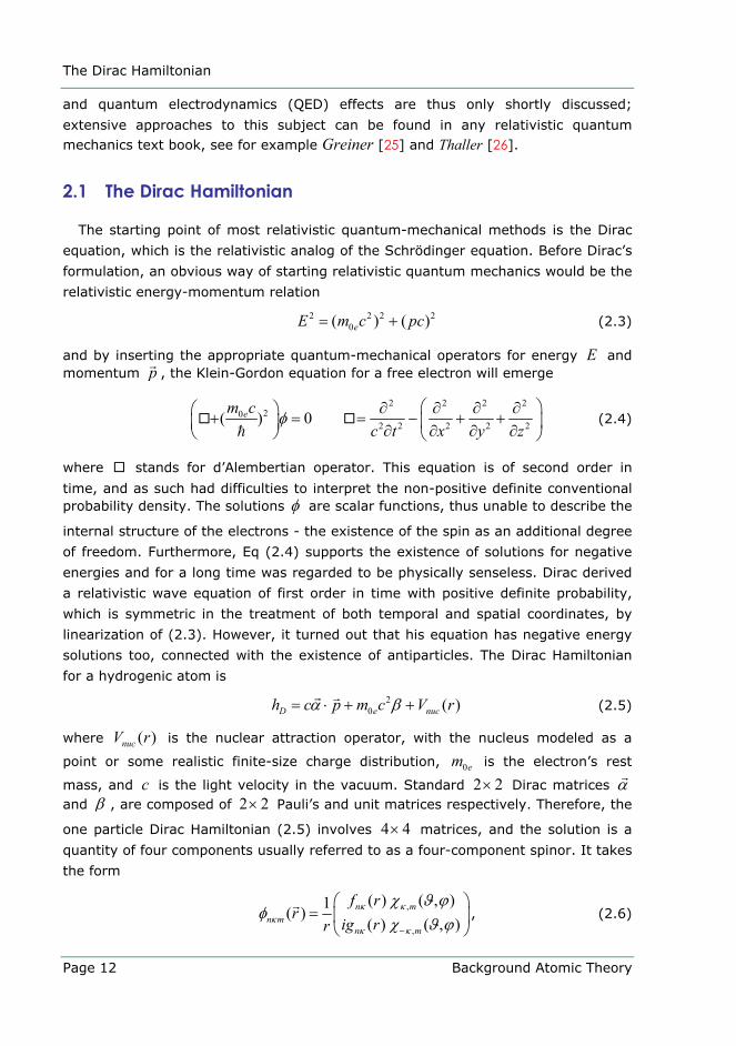
20 ( )D e nuch c p m c V rα β= ⋅ + + (2.5)
where ( )nucV r is the nuclear attraction operator, with the nucleus modeled as a
point or some realistic finite-size charge distribution, 0em is the electron’s rest
mass, and c is the light velocity in the vacuum. Standard 2 2× Dirac matrices α and β , are composed of 2 2× Pauli’s and unit matrices respectively. Therefore, the
one particle Dirac Hamiltonian (2.5) involves 4 4× matrices, and the solution is a
quantity of four components usually referred to as a four-component spinor. It takes
the form
,
,
( ) ( , )1( )( ) ( , )
n mn m
n m
f rr
ig rrκ κ
κκ κ
χ ϑ ϕφ
χ ϑ ϕ−
⎛ ⎞= ⎜ ⎟
⎝ ⎠, (2.6)

The Dirac Hamiltonian
Background Atomic Theory Page 13
where
1, 1/ 22
1/ 2( , ) ( ; , ) ( , )m
m C j m Y σ σκ λ
σ
χ ϑ ϕ σ σ ϑ ϕ−
=±
= − Ξ∑ , (2.7)
with mY σλ
− as a spherical harmonic, and
1/ 2 1/ 21/ 2 1/ 2
1 00 1
−⎛ ⎞ ⎛ ⎞Ξ = Ξ =⎜ ⎟ ⎜ ⎟
⎝ ⎠ ⎝ ⎠ (2.8)
are Pauli spinors; 12( ; , )C j m σ σ− are the Clebsch-Gordan coefficients, κ and λ
are the relativistic quantum numbers, defined as
12 1
21 12 2
( )( )
jif j
κλ κ
= ± ±=
= ± +∓
∓. (2.9)
Usually, the largest contributions to the positive energy (electronic) solutions are
coming from the first two components of (2.6), and a much smaller contribution
from the second two. Consequently, the upper half of Dirac’s spinor (2.6) is known as the large component, and the lower half is known as small component. For
positronic solutions, the opposite holds. The coupled radial differential equations for the large ( )nf rκ and small ( )ng rκ components are
2
0
( )( ) ( )( ) ( )
( ) 2
nucn n
n nnuc e
dV r cf r f rdr rg r g rdc V r m c
dr r
κ κ
κ κ
κ
εκ
⎛ ⎞⎛ ⎞− −⎜ ⎟⎜ ⎟ ⎛ ⎞ ⎛ ⎞⎝ ⎠⎜ ⎟ =⎜ ⎟ ⎜ ⎟⎜ ⎟⎛ ⎞ ⎝ ⎠ ⎝ ⎠+ −⎜ ⎟⎜ ⎟⎝ ⎠⎝ ⎠
(2.10)
where the total energy is taken to be 20eE m cε= + , and the normalization condition
has a form:
( )2 2
0
( ) ( ) 1n nf r g r drκ κ
∞
+ =∫ . (2.11)
Solutions to the system of radial equations (2.10) in the field free case
( ( ) 0nucV r → ), have a continuous energy spectrum with a gap between 202 em c− and
0 . Positive continuous eigenvalue spectrum 0ε > corresponds to free electron
solutions, while for 202 em cε < − positron continuum states occur. In the background
field of a Coulomb potential, the solutions that tend to vanish at the origin and at
the infinity, exist only for certain discrete energy values in 202 0em c ε− < < interval.
In the non-relativistic limit, c → ∞ , the two coupled radial Dirac equations (2.10)
reduce to the Schrödinger equation if the small components ng κ are eliminated.
Thus, the small component is a measure of the magnitude of relativistic effects.
No-virtual-pair approximation
Page 14 Background Atomic Theory
2.2 No-virtual-pair approximation
The conventional procedure of extending the non-relativistic many-body methods
to the relativistic domain, directly adding Coulomb repulsion to the independent-
particle Dirac equation (2.5), raises the problem of the negative energy continuum
states [27]:
“… It was proposed to get over this difficulty, making use of Pauli’s Exclusion Principle which does not allow more than one electron in any state, by saying that in the physical world almost all the negative-energy states are already occupied, so that our ordinary electrons of positive energy cannot fall into them. The question then arises to the physical interpretation of the negative–energy states, which on this view really exist. We should expect the uniformly filled distribution of negative–energy states to be completely unobservable to us, but an unoccupied one of these states, being something exceptional, should make its presence felt as a kind of hole. It was shown that one of these holes would appear to us as a particle with a positive energy and a positive charge and it was suggested that this particle should be identified with a proton. Subsequent investigations, however, have shown that this particle necessarily has the same mass as an electron and also that, if it collides with an electron, the two will have a chance of annihilating one another much too great to be consistent with the known stability of matter. It thus appears that we must abandon the identification of the holes with protons and must find some other interpretation for them. Following Oppenheimer, we can assume that in the world as we know it, all, and not merely nearly all, of the negative–energy states for electrons are occupied. A hole, if there were one, would be a new kind of particle, unknown to experimental physics, having the same mass and opposite charge to an electron. We may call such a particle an anti–electron. We should not expect to find any of them in nature, on account of their rapid rate of recombination with electrons, but if they could be produced experimentally in high vacuum they would be quite stable and amenable to observation. An encounter between two hard γ –rays (of energy at least half a million volts) could lead to the creation simultaneously of an electron and anti-electron, the probability of occurrence of this process being of the same order of magnitude as that of the collision of the two γ –rays on the assumption that they are spheres of the same size as classical electrons. This probability is negligible, however, with the intensities of γ –rays at present available.”
This model of occupied negative-energy states, also forbids the non-radiative
scenario where two initially positive energy electrons share available energy in the
way that one of them, by lowering the other into the negative-energy continuum,
increases its positive energy (“Auger effect”). On the other hand, Dirac’s theory
allows virtual excitations from the negative energy states (electron-positron pair
creation) as an effect of 3 Ryα [28].
The most commonly used approximation in the atomic structure calculations, is
that the vacuum is empty - it contains no virtual pairs. One way to achieve this is
the use of projection operators, constructed from eigenfunctions belonging to the
positive-energy branch of Dirac-Fock spectrum. By wrapping the electrostatic
electron-electron interaction 112r− with projection operators, negative-energy states
are projected out completely and, the no-virtual-pair approximation is introduced.
Breit interaction
Background Atomic Theory Page 15
2.3 Breit interaction
In the non-relativistic treatment of a many-electron system, the inclusion of
electrostatic interaction between the electrons is straightforward, see Eq (2.2).
However, for a relativistic description of electron-electron repulsion, the classical
instantaneous Coulomb interaction is deficient. Beside the fact that it is non-
covariant, it neglects the magnetic properties of the electron coming from the spin.
Additionally, retardation effects are expected to appear since the speed of light is
finite in a relativistic model. The covariant interaction in Coulomb gauge however,
has for its leading term exactly the classical instantaneous Coulomb interaction that
has to be modified in order to obtain higher approximations. These modifications are
derived from field theory (QED) as perturbation series with order parameter being the fine structure constant α .
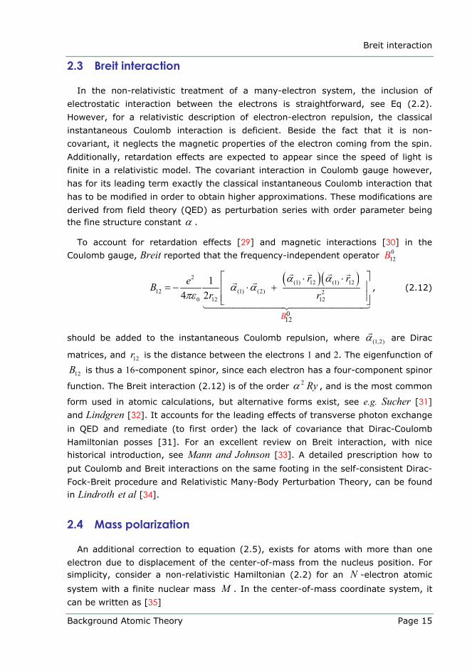
To account for retardation effects [29] and magnetic interactions [30] in the
Coulomb gauge, Breit reported that the frequency-independent operator 012B
( )( )2
(1) 12 (1) 1212 (1) (2) 2
0 12 12
012
14 2
B
r reBr r
α αα α
πε
⎡ ⎤⋅ ⋅⎢ ⎥= − ⋅ +⎢ ⎥⎣ ⎦
, (2.12)
should be added to the instantaneous Coulomb repulsion, where (1,2)α are Dirac
matrices, and 12r is the distance between the electrons 1 and 2. The eigenfunction of
12B is thus a 16-component spinor, since each electron has a four-component spinor
function. The Breit interaction (2.12) is of the order 2 Ryα , and is the most common
form used in atomic calculations, but alternative forms exist, see e.g. Sucher [31]
and Lindgren [32]. It accounts for the leading effects of transverse photon exchange
in QED and remediate (to first order) the lack of covariance that Dirac-Coulomb
Hamiltonian posses [31]. For an excellent review on Breit interaction, with nice historical introduction, see Mann and Johnson [33]. A detailed prescription how to
put Coulomb and Breit interactions on the same footing in the self-consistent Dirac-
Fock-Breit procedure and Relativistic Many-Body Perturbation Theory, can be found in Lindroth et al [34].
2.4 Mass polarization
An additional correction to equation (2.5), exists for atoms with more than one
electron due to displacement of the center-of-mass from the nucleus position. For simplicity, consider a non-relativistic Hamiltonian (2.2) for an N -electron atomic
system with a finite nuclear mass M . In the center-of-mass coordinate system, it
can be written as [35]
Radiative corrections
Page 16 Background Atomic Theory
2
2
1 10
1| |
1 1/2 4
N N N N
i i i ji i i j i ji jr r
eH p Z r p pMµ πε= = < <
−⎛ ⎞
= + − + +⎜ ⎟⎝ ⎠
∑ ∑ ∑ ∑ (2.13)
where µ is the reduced mass ( 0 0/( )e eM m M mµ = + ). Equation (2.13) differs, to
start with, from the Hamiltonian (2.2) for an infinitely heavy nucleus in that the kinetic energy term in (2.13) contains µ instead of the electron rest mass 0em . This
term is called the normal mass shift, and arises from the motion of the nucleus due
to its finite mass, contributing to the positive energy shift. The next difference is the
last term on the right-hand side of (2.13), which refers to the momentum
correlations between pairs of electrons orbiting the nucleus, and gives a rise to the specific mass shift or mass polarization. It is described by the two-particle operator,
and treated as a perturbation. Its contribution to the level energy is obtained with
first-order perturbation theory as
(1/ )mp i ji j
E M p p<
∆ = ⋅ ∑ (2.14)
where, the angular brackets in the right side of (2.14) denote an expectation value
over the (infinite nuclear mass) zero-order wave function, and its sign depends on
the electronic state.
2.5 Radiative corrections
The hydrogenic states with the same n and j quantum numbers, but different
quantum numbers, ought to be degenerate, according to Dirac’s theory. The famous 1947 experiment by Lamb and Retherford [36] used a microwave technique to
determine the splitting between 21/ 22 S and 2
1/ 22 P states in hydrogen. They showed
that the 21/ 22 S state had slightly higher energy by an amount (Lamb shift) now
known to be 1057.864 MHz .
The effect is explained by the QED theory, and the Lamb shift today commonly
refers to the radiative QED effects that appear first in order 4 3 3Z n Ryα − . In the QED
theory, the electro-magnetic field itself is quantized, with non-zero energy of its ground state. The field instead undergoes vacuum fluctuations (creating electron-
positron pairs or virtual photons seemingly out of nothing) that interact with the
charged particles. Any discussion of the calculation is beyond the scope of this
thesis, but in a rather simplified way, we can view it as follows.
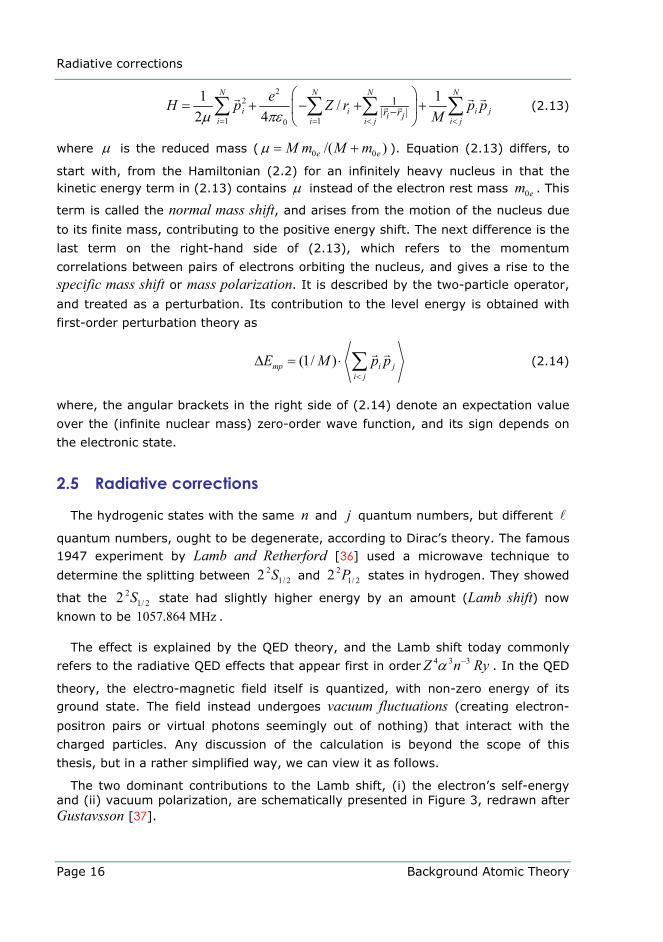
The two dominant contributions to the Lamb shift, (i) the electron’s self-energy and (ii) vacuum polarization, are schematically presented in Figure 3, redrawn after Gustavsson [37].
Radiative corrections
Background Atomic Theory Page 17
Figure 3 Illustration of two dominant QED effects beyond the RMBPT used in Papers II and I.
The self energy of a free electron, if seen as a uniformly charged sphere of
classical electron’s radius, is of the order 20em c . The self-energy is commonly
regarded as energy needed to “assemble” an electron due to the interaction with its
own radiation field (a virtual photon is emitted then reabsorbed). This energy may
change when the electron is in a bound state, in a way similar as to increase the
electron’s mass. That change (renormalization of the electron’s mass) should be
accounted for in energy level calculations.
Vacuum polarization is the descriptive term of the short-range modifications of
the Coulomb’s law. A charged particle will polarize the vacuum in a way analogous
to the way a dielectric is polarized, effectively reducing its charge. Namely, a virtual
electron-positron pair in the vacuum will be affected by the presence of a charged
particle. If it is an electron, the positron will be attracted and the virtual electron
repelled, causing a net polarization of the vacuum, which screens the electron's
charge. The vacuum polarization correction for an electron in a nuclear Coulomb field, is accounted for by adding the Uehling correction [38] to the Coulomb potential. It is interesting to note that the fine-structure “constant” α (as the
measure of the strength of the electromagnetic force, that governs how electrically
charged elementary particles and radiation field interact) will vary a bit with
distance and therefore with energy.
The nuclear size corrections (field shift) also contribute to the original Lamb shift,
since due to it, a small difference in energy arises between 21/ 22 S and 2
1/ 22 P
hydrogen states. Different models for the nuclear charge distributions exist, and detailed description of those used in Papers II and I, can be found in Nikolić [39].

Dragan Nikolié Page 19
Chapter 3 Reduced Hamiltonians
In physics, as an analytical deductive science starting from general principles and
simplifying assumptions, it is possible to predict explicit relations among physical
quantities in form of laws and models. The many-body problem in atomic physics is
difficult because of the long-range nature of the Coulomb interaction. This type of
problem, even when relativity is neglected, cannot be treated without approximation
on today’s supercomputers.
The urge to provide more and more significant digits to experimentalists gave birth to efficient ab initio numerical computational techniques, that are able to
diagonalize approximate Hamiltonians, delivering eigenvalues and eigenvectors
spread on a vast number of model configurations. Hindered by the enormous
amount of information, the understanding of the underlying physics is tightly
connected to the reduction of obtained results using simplifying schemes.
One of those simplifying schemes is the effective Hamiltonian formalism by Bloch,
based on the idea to include the effect of the perturbation in the operator rather
than in the wavefunctions. The effective operator acts in the limited space and
reproduces there exactly the effect of the true operator. The basis for our many-body treatment of the effective Hamiltonian is the procedure described in Lindgren and Morrison [40]. Ref. [40] describes in particular how to handle many-electron
atoms with one or two open shells and our studies of dielectronic recombination
(Papers II and I) follow it closely, see Chapter 4.
The intruder state problem in applications of multireference perturbation and
coupled cluster theory, see for example [41, 42], is widely recognized as the main
obstacle for universal applicability of the effective Hamiltonian formalism. So it is not surprising that we encountered the same difficulties, see Lindroth [43] and
Paper III. This chapter discusses a method to avoid this problem.
In general, doubly excited states are states with two open shell electrons. I will
thus concentrate only on this particular problem, but in principle, there can be a
Reduction by projection technique
Page 20 Reduced Hamiltonians
closed shell core in addition to the two electrons in open shells. Additional diagrams
will then have to be considered, but here I will for simplicity discuss only pure two-
electron systems.
I shall proceed as follows. In §3.1 the basics of Bloch’s formalism of the effective
Hamiltonians in finite model spaces will be presented. An introduction to the intruder
state problem is given in §3.2, along with a presentation of existing ways of avoiding
it using intermediate Hamiltonians. Next, in §3.3, I will show how to formulate the
concept of state selective Hamiltonian and avoid specific types of intruder states.
Contrary to most implementations of the effective Hamiltonian formalism [40,
66,43], I will chose to work with functions coupled to a specific total angular
momentum and spin.
3.1 Reduction by projection technique
The main idea is to reduce the exact Hamiltonian to a simplified Hamiltonian,
which describes only a restricted part of the total spectrum. A first contribution to such a transformation came from Van Vleck [44]. Other authors followed with
different transformations, see for example Jordahl [45] and Soliverez [46], but the
most fundamental transformations resulting in effective Hamiltonians are those of
Bloch [47] and des Cloizeaux [48]. The term “effective” denotes that the
Hamiltonian is obtained by projecting exact wavefunctions onto a finite model space, which is a D
0S -dimensional subspace, 0S , of the entire Hilbert space.
The first to generalize the original Bloch equation [47] (derived for exact degenerate states) for quasi-degenerate systems was Jørgensen [49]. Based on an explicit partition of the full Hamiltonian H into an model Hamiltonian 0H and a
perturbation V , Lindgren [50] established an even more general Bloch equation.
The central point in the generalizations above is the concept of a finite model space and an associated wave operator Ω from which the effective Hamiltonian can be
found. Finally, Durand [51] showed how the above techniques can be generalized into one compact canonical wave-operator equation, derived without any partition
of the full Hamiltonian.
In order to proceed, additional terminology has to be introduced. The model space
0S has its orthogonal complement ⊥0S , usually referred to as outer space, both
associated with orthogonal projection operators, 0P and 0Q , respectively:
0 0 0 0 1m
m mγ
γ γ∈ ∉
= = + ≡∑ ∑ 0 0S S
P Q P Q , (3.1)
where the functions used to span model space are labeled with Latin letters, and
those spanning the outer space are labeled in Greek. Note that Paper III use slightly
Reduction by projection technique
Reduced Hamiltonians Page 21
different labels for projection operators 0( )P ≡ P and 0( )Q ≡ Q . For the sake of
clarity and without loss of generality, we can assume that the two-electron Hamiltonian H can be divided into an unperturbed part 0H (consisting of a sum of
one-particle Hamiltonians, 0h , with a known spectrum whose eigenstates are
orthogonal by construction), and a perturbation V :
2
0 0 01
0 ( , )
( )
(1,2)p
k k k k n k n
H H V H h p
h φ ε φ φ φ δ=
= + =
= =
∑ (3.2)
We use the one-electron eigenfunctions kφ to construct antisymmetrized two-
electron functions coupled to a specific total symmetry 2 1S Lπ+ , with the purpose to
span the model space through Eq.(3.1):
1 ( 1, 2)
1 2 1 2 2 1
1 2
1(1) (2) ( 1)2
m
exchange partdirect partm m
m m m m m mLS LS
m m m
m
m
L S
δϕφ φ φ φ φ φ
ϕπ
+ ⎡ ⎤⎛ ⎞ ⎢ ⎥≡ = + −⎜ ⎟ ⎢ ⎥⎝ ⎠ ⎣ ⎦
= + + +
A, (3.3)
where A … stands for an antisymmetrized product and mπ is the parity of a given
two-electron function. The spanning functions m are inherently ortho-normalized
forming a complete basis set, as solutions of the unperturbed Hamiltonian 0H with
spectral resolution
0 , 1, 1 2, 21
0 0 0
0 0 0
,D
m m m mm D
H
H
H m m γ γ γ γγ
ε γ ε γ ε ε ε= >
= + = +∑ ∑
Q Q
P P
S 0
S 0
. (3.4)
Using selected solutions mΨ of the full Hamiltonian H ,
1,2,m m mH E m DΨ = Ψ =0S… , (3.5)
one can span a subspace S with the same dimensionality D0S that corresponds to
the part of the total spectrum in which we are interested. As depicted in Figure 4,
redrawn from Durand [51], ⊥S is the orthogonal complement of S . The aim is to
pass from the full Hamiltonian H to an effective Hamiltonian effH , whose
eigenvalues coincide with the S subset of eigenvalues of H , losing the information
on all other eigenvalues. The main difficulty of Bloch [47] and des Cloizeaux [48]
effective Hamiltonians comes from the wave operator that explicitly depends on the target space projector, see review of Durand and Malrieu [52]. It is not difficult to
Reduction by projection technique
Page 22 Reduced Hamiltonians
choose the model space 0S on which the reduced quantum information will be
projected, but the target space S is not a priori known. If the energy levels
associated with the model space are well separated from the rest of the spectrum,
the coupling between 0S and ⊥0S is small for the exact Hamiltonian H , and the
identification of the target space S is unambiguous. The knowledge of S is less
accessible when strong coupling between 0S and ⊥0S exists, for example due to
intruder states. Depending on the existence and type of crossings of energy levels
associated with intruder and model states, see Figure 8 for an illustration, the
effective Hamiltonian has discontinuities in the physical content of its solutions (the adiabatic situation) or in its energies (the diabatic situation). In practice, the target space S covered by Bloch [47] and des Cloizeaux [48] effective Hamiltonians,
relies on two criteria; one is the (adiabatic) energetic criterion, which selects the D
0S lowest states of a given symmetry. With an alternative (diabatic) criterion, the
D 0S states are chosen so that their occupation 0Ψ ΨP in the model space, 0S , is
maximized.
Figure 4 The full, effective, intermediate and state selective Hamiltonians have the same eigenvalues in the finite subspaces S , 0S and MS , while the information on states residing in ,
⊥0 2S spaces is lost. Indicated levels
belonging to the complementary ,⊥0 2S spaces are eigenvalues of the model Hamiltonian 0H . The intermediate IS
and ⊥ 1S spaces act as buffer zones where state selective Hamiltonian ssH disregards any quantum information,
while intermediate Hamiltonian intH reproduces only approximate eigenvalues.
Reduction by projection technique
Reduced Hamiltonians Page 23
The central role in the theory of effective Hamiltonians is played by the one-to-one correspondence between target S and model 0S space functions, established by
model functions mΦ as projections of the exact solutions mΨ onto the model
space
0
1,2,m m m D∈ ∈
ΩΨ Φ = 0
0
S S
S…P
. (3.6)
With this correspondence, a single wave operator Ω transforms all model functions
back into the corresponding exact functions, and as such is crucial for the concept of effective Hamiltonian effH . As illustrated by Figure 4, the Bloch formalism requires
that the D 0S solutions of effH in the model space must be the projections on the
model space of the D0S exact solutions mΨ spanning the target space S :
0 1,2,effm m
m m mm m
H E m DΦ = Ψ
Φ = Φ =Ψ = Ω Φ 0S…
P (3.7)
The wave operator Ω , associated with the exact solutions mΨ , acts entirely in
model space and obeys the canonical equation of Durand [51]
[ , ] 0H Ω Ω = , (3.8)
which under partitioning (3.2) of the full Hamiltonian H reproduces the generalized Bloch equation of Lindgren [50]
[ ]0 0 0 0 0, H V VΩ = Ω − Ω ΩP P P P , (3.9)
having the following decomposition
0 0 0 0
0
( )χ
Ω = + Ω = Ω + ΩP
P Q P Q , (3.10)
where the property 0 0Ω =P P is equivalent to the so-called intermediate normalization, and 0 0χ χ= Q P is a correlation operator that couples model space
and outer space. Intermediate normalization means that only the part of the exact
wavefunction lying in the model space is normalized. It is obvious that the wave
operator (3.10) does not depend on unknown target space functions (3.5), as is the case in the original method of Bloch [47] and des Cloizeaux [48]. Therefore, any D
0S subsequent states of a given symmetry in an energy range of interest can
constitute the target space S . The stationary occupancies Φ Ω Φ are a reliable
indicator for the quality of the model space 0S ; if the choice of the model space is
inadequate or an intruder state problem exists, during solution of (3.9) their values
will change noticeably, as a signature of divergence.
Reduction by projection technique
Page 24 Reduced Hamiltonians
The generalized Bloch equation (3.9) can be transformed into a commutator equation for the correlation operator χ , which can be solved recursively:
1 00 0 0 0, (1 ) (1 ) , 0 , 0,1,s s s sH V sχ χ χ χ+ =⎡ ⎤ = − + = =⎣ ⎦ …P Q P (3.11)
where s denotes recursion stages. The numerical solution of Eq. (3.11) with the
basis (3.4) of the unperturbed Hamiltonian 0H , relies on the recursive solution of a
set of D 0S coupled equations for the pair-functions m mρ χ=
1 0 0
1,
0,1,( )
1,2,
m
s s s sm m m j m
j D
s
sH V m j V m
m Dε ρ ρ ρ ρ
∈+
=
=− = + − +
=∑ 0
0S 0
S
S…
……
Q
RHS
(3.12)
where smRHS denotes the right-hand side of the equation for a given recursion
stage. Acting from the left on (3.12) with resolvent 0mQR , having the spectral
resolution
0 0 01 1 0 0 0( ) ( ) ,m m m m m
mH γ
γ
ε γ ε ε γ⊥∈
− −
≠
= − = − =∑Q Q QR Q R Q R 0S
(3.13)
one obtains a coupled system of equations for the pair-functions:
1 10
1,2,( )
0,1,2,s s
m m mm
m D
sγγ
ρ γ ε ε γ⊥∈
+ −
≠
== −
=∑
0 0
SS…
…Q RHS (3.14)
The spin-angular part of (3.14) can be solved analytically, while the radial part has
to be treated numerically in an iterative manner until (if) a satisfactory convergence
is achieved.
The construction of the effective Hamiltonian starts with the application of 0P
from the left on the exact eigen-problem (3.5), and using the correspondence (3.6) one can get Eq.(3.7), with effV as an effective perturbation:
00 0 0 0 0 0 0 0 0
0 0 0 0eff eff eff
0 effeffVHH
H H H H V H Vχ
χ χ=
= Ω = + + = +P P
P P P P P P P P . (3.15)
The spectral resolution of the zero-stage effective Hamiltonian 0effH is
0 0 0( , )
1
0( )
eff
effD
m m k m mm
kmH
H m E m E Diag k V mδ ε=
= ↵ ∴ +∑S 0
, (3.16)
where zero stage energies 0mE are a result of the diagonalization of 0( )eff kmH matrix.
Intruder state problem and intermediate Hamiltonians
Reduced Hamiltonians Page 25
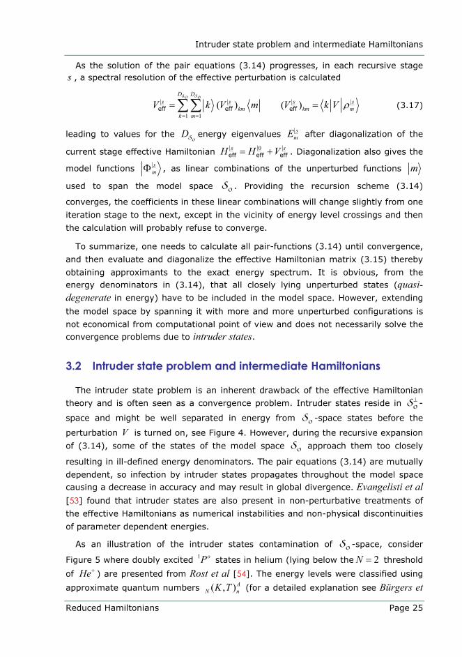
As the solution of the pair equations (3.14) progresses, in each recursive stage s , a spectral resolution of the effective perturbation is calculated
1 1
( ) ( )eff eff eff
D Ds s s s
km km mk m
V k V m V k V ρ= =
= =∑ ∑S S 0 0
(3.17)
leading to values for the D0S energy eigenvalues s
mE after diagonalization of the
current stage effective Hamiltonian 0eff eff effs sH H V= + . Diagonalization also gives the
model functions smΦ , as linear combinations of the unperturbed functions m
used to span the model space 0S . Providing the recursion scheme (3.14)
converges, the coefficients in these linear combinations will change slightly from one
iteration stage to the next, except in the vicinity of energy level crossings and then
the calculation will probably refuse to converge.
To summarize, one needs to calculate all pair-functions (3.14) until convergence,
and then evaluate and diagonalize the effective Hamiltonian matrix (3.15) thereby
obtaining approximants to the exact energy spectrum. It is obvious, from the energy denominators in (3.14), that all closely lying unperturbed states (quasi-degenerate in energy) have to be included in the model space. However, extending
the model space by spanning it with more and more unperturbed configurations is
not economical from computational point of view and does not necessarily solve the convergence problems due to intruder states.
3.2 Intruder state problem and intermediate Hamiltonians
The intruder state problem is an inherent drawback of the effective Hamiltonian
theory and is often seen as a convergence problem. Intruder states reside in ⊥ 0S -
space and might be well separated in energy from 0S -space states before the
perturbation V is turned on, see Figure 4. However, during the recursive expansion
of (3.14), some of the states of the model space 0S approach them too closely
resulting in ill-defined energy denominators. The pair equations (3.14) are mutually
dependent, so infection by intruder states propagates throughout the model space causing a decrease in accuracy and may result in global divergence. Evangelisti et al [53] found that intruder states are also present in non-perturbative treatments of
the effective Hamiltonians as numerical instabilities and non-physical discontinuities
of parameter dependent energies.
As an illustration of the intruder states contamination of 0S -space, consider
Figure 5 where doubly excited 1 oP states in helium (lying below the 2N = threshold
of He+ ) are presented from Rost et al [54]. The energy levels were classified using
approximate quantum numbers ( , )AN nK T (for a detailed explanation see Bürgers et
Intruder state problem and intermediate Hamiltonians
Page 26 Reduced Hamiltonians
al [55] and references therein). N and n are principal quantum numbers of the
inner and outer electrons, respectively. The quantum number K describes angular
correlation between electrons and is related to the interelectronic angle, while
T comes from the quantization of the projection of total angular momentum L
along the axis N nb b− , where b is the Runge-Lentz vector. The Pauli principle and
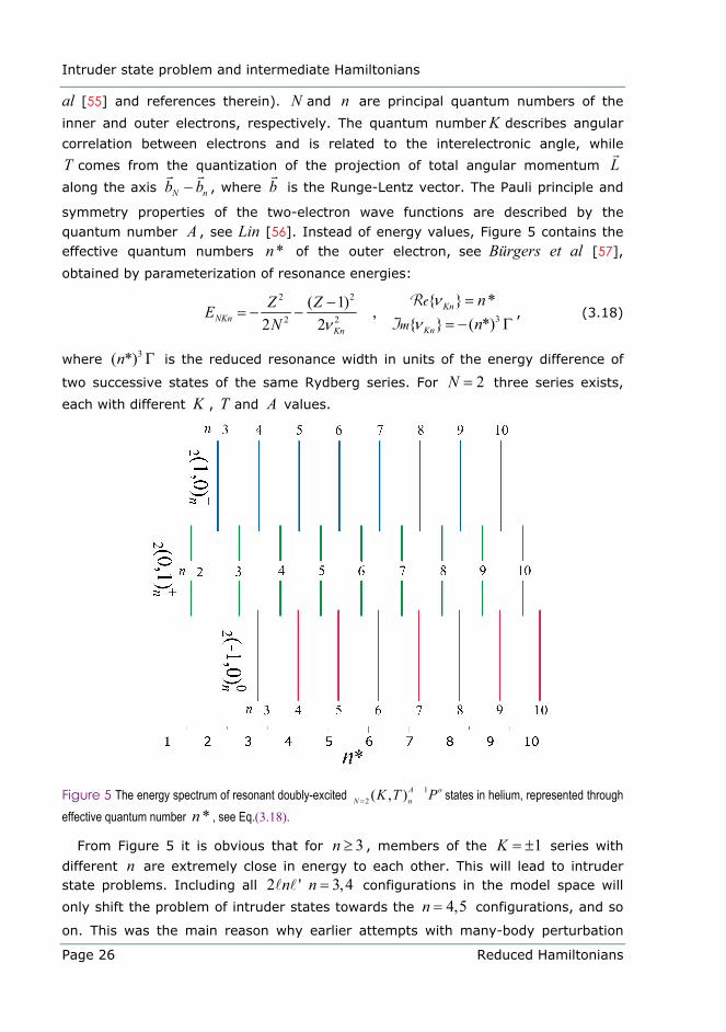
symmetry properties of the two-electron wave functions are described by the quantum number A , see Lin [56]. Instead of energy values, Figure 5 contains the effective quantum numbers *n of the outer electron, see Bürgers et al [57],
obtained by parameterization of resonance energies:
2 2
32 2
*( 1) , ( *)2 2
KnNKn
KnKn
nZ ZEnN
ννν
=−= − −
= − ΓRe
Im, (3.18)
where 3( *)n Γ is the reduced resonance width in units of the energy difference of
two successive states of the same Rydberg series. For 2N = three series exists,
each with different K , T and A values.
Figure 5 The energy spectrum of resonant doubly-excited 12 ( , )A o
N nK T P= states in helium, represented through effective quantum number *n , see Eq.(3.18).
From Figure 5 it is obvious that for 3n ≥ , members of the 1K = ± series with
different n are extremely close in energy to each other. This will lead to intruder state problems. Including all 2 ' 3,4n n = configurations in the model space will
only shift the problem of intruder states towards the 4,5n = configurations, and so
on. This was the main reason why earlier attempts with many-body perturbation
Intruder state problem and intermediate Hamiltonians
Reduced Hamiltonians Page 27
theory, see Lindroth [43], failed to obtain precise energy positions and widths for
2 3( , )AN K T= states of 1 oP symmetry in helium.
At this point, it is interesting to quote Evangelisti et al [53]: “… The intruder state problem, as a recurrent dilemma, cannot be solved by enlarging the model space. Another type of solution is needed.” The first formulation of the intermediate Hamiltonians intH concept by Malrieu et al [58], see Figure 4, was oriented towards
degenerate perturbation theory applications. It was originally developed to overcome the convergence difficulties, which effective Hamiltonian, Heff, experienced
in the region of intruder states. Heully et al [59] have proposed a similar method in
the framework of quasidegenerate perturbation theory. Non-perturbative intermediate schemes also exist: a coupled-cluster approach of Mukhopadhyay et al [60] and Meissner [61], as well as configuration interaction approach of Daudey et al [62], to name a few of them.
The approach of intermediate Hamiltonian intH introduces a partitioning of the
model space 0S , which is a priori divided into a DMS dimensional main model space
MS and D D D= −I 0 MS S S dimensional intermediate model space IS . Associated
projectors are, in accordance with (3.1), given by
0M I M Im i
m m i i∈ ∈
= = + ≡∑ ∑ M IS S
P P P P P , (3.19)
i.e., spanned by appropriate solutions (3.3) of the unperturbed Hamiltonian (3.4).
Less ambitious requirements, from those imposed to effective Hamiltonian (3.7), are
expected from the intermediate Hamiltonian
0
0
1,2,( )
int
m m
m m m m m
M I M
H E m DΦ = Ψ
Φ = Φ Ψ = Ω Φ =Ω ≡ + + Ω
MS…P
P Q P P (3.20)
since the other eigenenergies 1,2,inti iE E i D≠ =
IS… are only approximate, as an
acceptable price to pay for the good convergence for MS states. Exact
reproducibility, as given by (3.20), is achieved by simultaneous introduction of the ordinary wave operator Ω , see Eq. (3.6), acting now only in the main MS model
space, and a non-orthogonal projector 0R R= P that acts on both MS and IS .
Considering the main model space MS as degenerate with a common energy 0ε , Malrieu et al [58] demonstrated that the projector R satisfies the fundamental
relation
00 0 (1 )R VR= − ΩQQ R (3.21)
Intruder state problem and intermediate Hamiltonians
Page 28 Reduced Hamiltonians
where 0 10 0 0 0( )Hε −= −QR Q represents the resolvent analogous to (3.13), with
parameterized spectral resolution (3.4) of the unperturbed Hamiltonian
0 0 1 1
0 0 0
0 0
D D
im i D D
M M I I
H
H H
H m m i i γγ
ε ε γ ε γ= = + >
= + +∑ ∑ ∑S S M 0
S S M 0
Q Q
P P P P
. (3.22)
The intermediate Hamiltonian itself satisfies a relation similar to (3.15)
0 0intH HR= P P , (3.23)
and its diagonalization in +M IS S space provides a set of eigenvalues (3.20) of
which only a subset associated to the main MS model space is equivalent to that
reproduced by the effective Hamiltonian (3.7). The main reason why this diagonalization involves states in IS is not to gain additional eigenvalues, but to
include the contributions from the intermediate space in a safe way (through diagonalization) and not via the wave operator Ω (now sustained in MS ).
Perturbative expansion of (3.21) involves energy denominators associated with
excitations from the main model space MS to intermediate IS and outer ⊥ 0S
spaces, but never between IS and ⊥0S . This property resolves the convergence
problems when intruder states from outer space enter the intermediate energetic region, see Evangelisti et al [53], since tunable parameter 0ε should provide
sufficient energy separation between MS and IS or ⊥0S spaces. The main
disadvantage of this approach is that in reality it is often impossible to isolate an energetic region corresponding to the main model space MS . As pointed out by
authors, see Malrieu et al [58] Appendix 1, perturbative expansion of (3.23) contains dangerous →M IS S excitations (through I MΩP P part of Ω ) in fourth3
and higher orders, and difficulties may appear if some of the intermediate
configurations are strongly coupled to those of the main model space, as illustrated on Figure 4. To address this problem, Heully et al [59] considered different
schemes; these attempts may lead to completely new methods, but often uncover
new ways of solving the basic relation (3.21). Nevertheless, what remains is awareness of the dangerous I MΩP P term, which has to be isolated from equations
(3.21) and (3.23).
Reformulating the Fock-space coupled-cluster method in the spirit of intermediate Hamiltonian, Landau et al [63] eliminated the I MΩP P term from central equations,
3 Contributions from ⊥1S also starts to couple in fourth order, see Eq. (3.41).
State selective Hamiltonian
Reduced Hamiltonians Page 29
and removed the main obstacle for the implementation of intermediate Hamiltonian
into the coupled-cluster methodology. However, as an inherited generalization feature of the original approach of Malrieu et al [58], an energy parameter E
remains, which Landau et al [63] chose to express as
occ.
jj
E Cε= +∑ (3.24)
where the sum goes over all occupied orbitals with corresponding energies jε . The
converged results are, in principle, independent of C which in addition can be tuned
to eliminate ill-defined energy denominators.
Inspired by the above-mentioned achievements, which demonstrated that
intruder-state infection of the upper part of the model space could be suppressed
using an intermediate Hamiltonian formalism, we developed a method (Paper III)
elaborated in the following section.
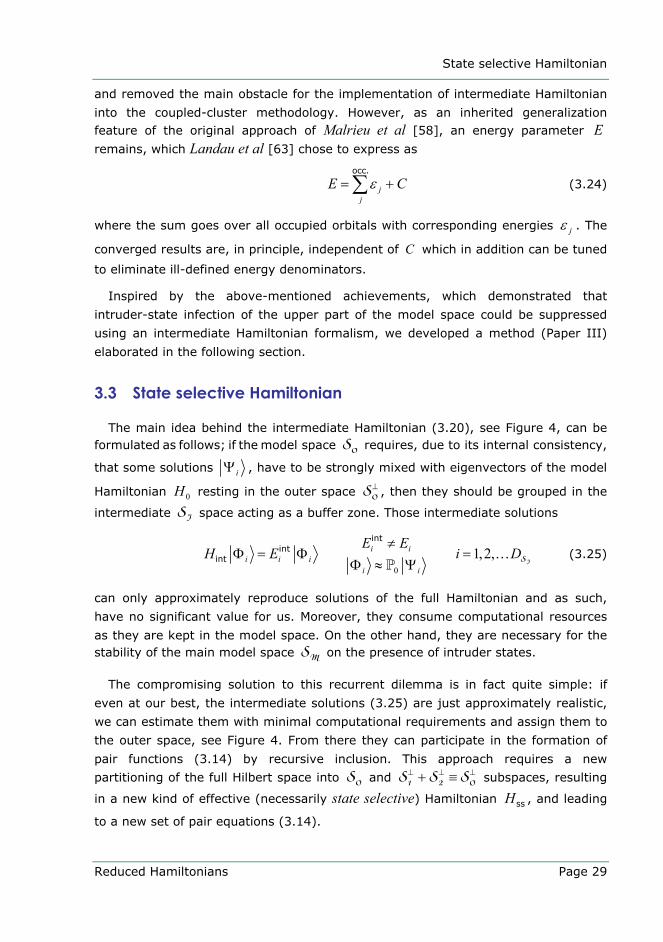
3.3 State selective Hamiltonian
The main idea behind the intermediate Hamiltonian (3.20), see Figure 4, can be formulated as follows; if the model space 0S requires, due to its internal consistency,
that some solutions iΨ , have to be strongly mixed with eigenvectors of the model
Hamiltonian 0H resting in the outer space ⊥0S , then they should be grouped in the
intermediate IS space acting as a buffer zone. Those intermediate solutions
0
1,2,int
intint
i ii i i
i i
E EH E i D
≠Φ = Φ =
Φ ≈ Ψ IS…P
(3.25)
can only approximately reproduce solutions of the full Hamiltonian and as such,
have no significant value for us. Moreover, they consume computational resources
as they are kept in the model space. On the other hand, they are necessary for the stability of the main model space MS on the presence of intruder states.
The compromising solution to this recurrent dilemma is in fact quite simple: if
even at our best, the intermediate solutions (3.25) are just approximately realistic,
we can estimate them with minimal computational requirements and assign them to
the outer space, see Figure 4. From there they can participate in the formation of
pair functions (3.14) by recursive inclusion. This approach requires a new
partitioning of the full Hilbert space into 0S and ⊥ ⊥ ⊥+ ≡1 2 0S S S subspaces, resulting
in a new kind of effective (necessarily state selective) Hamiltonian ssH , and leading
to a new set of pair equations (3.14).
State selective Hamiltonian
Page 30 Reduced Hamiltonians
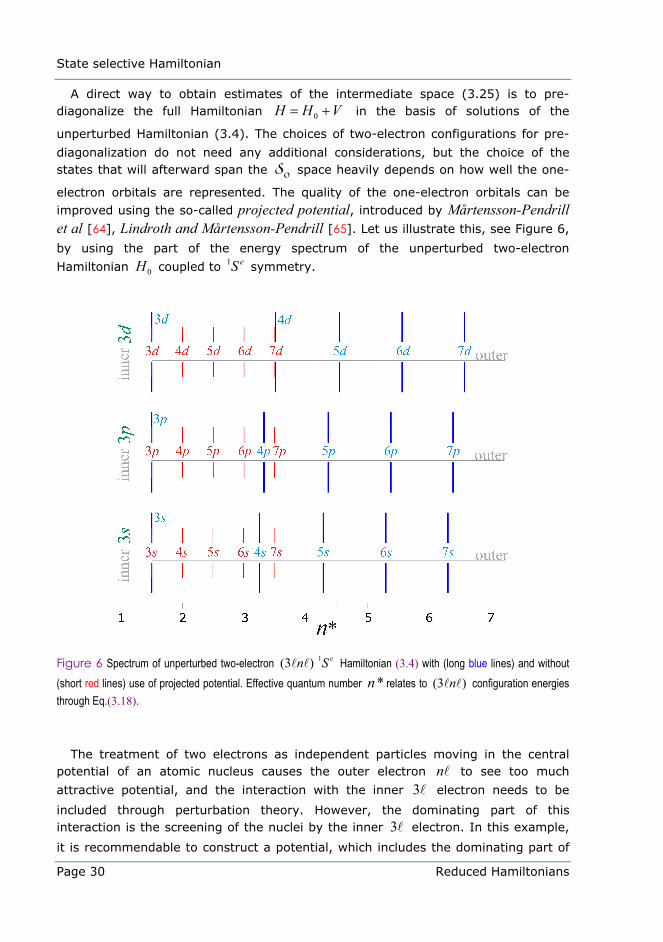
A direct way to obtain estimates of the intermediate space (3.25) is to pre-diagonalize the full Hamiltonian 0H H V= + in the basis of solutions of the
unperturbed Hamiltonian (3.4). The choices of two-electron configurations for pre-
diagonalization do not need any additional considerations, but the choice of the states that will afterward span the 0S space heavily depends on how well the one-
electron orbitals are represented. The quality of the one-electron orbitals can be improved using the so-called projected potential, introduced by Mårtensson-Pendrill et al [64], Lindroth and Mårtensson-Pendrill [65]. Let us illustrate this, see Figure 6,
by using the part of the energy spectrum of the unperturbed two-electron
Hamiltonian 0H coupled to 1 eS symmetry.
Figure 6 Spectrum of unperturbed two-electron 1(3 ) en S Hamiltonian (3.4) with (long blue lines) and without (short red lines) use of projected potential. Effective quantum number *n relates to (3 )n configuration energies through Eq.(3.18).
The treatment of two electrons as independent particles moving in the central potential of an atomic nucleus causes the outer electron n to see too much
attractive potential, and the interaction with the inner 3 electron needs to be
included through perturbation theory. However, the dominating part of this interaction is the screening of the nuclei by the inner 3 electron. In this example,
it is recommendable to construct a potential, which includes the dominating part of
State selective Hamiltonian
Reduced Hamiltonians Page 31
this screening while the inner 3 electron only sees the unscreened nucleus, see
Lindroth and Mårtensson-Pendrill [65]
( ) ( )23 ,3 ,3
312
, 1 ,2 ,21 3 3 1
4proj
s p ds
c c d dc d s s p o
eV s k r s kφ φ φ φπε=
= − − ≡∑ (3.26)
The restriction of preserving the Hermicity implies the non-locality of the projected
potential, which therefore has to be generated iteratively. As Figure 6 shows, with
the use of the projected potential 3proj
sV , a better description of the outer (4 7)n≤ ≤
electron provides more realistic energies for the 1(3 4 ) en S≥ configurations.
Using all fifteen 1(3 ) en S 3 7n≤ ≤ configurations shown in Figure 6 to
diagonalize the full Hamiltonian, fifteen eigenvalues and eigenstates are obtained
(see Figure 7). However, Figure 7 shows only the first thirteen since in order to parameterize the last two eigenvalues well, using Eq. (3.18), also 8n =
configurations have to be included.
Figure 7 The map of some of the 1 eS energy levels in helium used for testing purposes, see text. The ordering of diagonalized states labeled as (5) and (6) as well as (8) and (9) will eventually change.

State selective Hamiltonian
Page 32 Reduced Hamiltonians
How many of those fifteen pre-diagonalized states will span the model space 0S
depends on the previous knowledge and choice of the target space S . In the above
example, our intention is to obtain the nine lowest 3( , )AnK T states in helium of 1 eS
symmetry, where the known problem of recurrent intruder states occurs. An overview
of the doubly excited 1 eS states in helium, see Figure 8, can be found in Bürges et al [55], and some of them relevant for this example are marked as exact in Figure 7.
Figure 8 Effective quantum number ( e.g. resonance positions) of the 1 eS helium resonances bellow the 3N = threshold as a function of the relative strength of the electron-electron interaction. Figure is reproduced after Ref.[55].
State selective Hamiltonian
Reduced Hamiltonians Page 33
One can see that 3( 2,0)n+− doubly excited states (3 7n≤ ≤ ) are extremely close
in energy to the 3 2( 2,0)n+
++ states, which act as the intruder states if one wants to
include any subset of the 1(3 ) en S configurations to span the model space 0S
using (3.1). The corresponding eigenvalues of the unperturbed Hamiltonian (3.4) in
Figure 7 are labeled “unperturbed”, as the one-electron orbitals kφ , see Eq.(3.2),
are generated in the projected potential (3.26) coming from the inner 3s electron
and do not actually represent the solutions of two independent electrons.
Since the set of pair equations (3.14) contains the energy denominators
associated with ⊥→0 0S S excitations, and “unperturbed” solutions are spanning the
outer space ⊥0S , the choice of the model space 0S is governed by its energy
separation from the outer space ⊥ ⊥ ⊥= +0 1 2S S S . If we aim to arrive at the lowest
nine states in S starting from the lowest nine pre-diagonalized states in 0S , no
outer space states should come in between. This is true for the states associated
with the orthogonal ⊥1S space. The same holds for the states from ⊥
2S since all 1(3 ) en S 3 7n≤ ≤ configurations formally belong to 0S and cannot be present in
⊥ 2S . All outer space states of the same symmetry converging to lower 1N = and
2N = thresholds are also well isolated using the projected potential (3.26). This
example should provide basic insight of the new state selective approach and what
follows is a derivation of its main features.
So far, after pre-diagonalization of the full Hamiltonian 0H V+ , we have at our
disposal D D ⊥+ 0 1
S S energies mE and corresponding eigen-vectors m
kC
0
( , )11
1,2, ( )( ) i i i
D DD Dj ii
j i k k j ii kkk
i D DH V E
C CC k δ
⊥
⊥⊥ ++
==
= ++ Ψ = Ψ
Ψ Ψ = =Ψ = ∑∑
0 1
SS 0 0 SS 1 1
S S…
(3.27)
where iΨ are orthonormal spanning functions for the selected model 0S and
outer ⊥ 1S spaces, whose associated projectors are
0 11 1
D DD
m mm D
β ββ
⊥+
= = +
= Ψ Ψ = Ψ Ψ∑ ∑S 0S S 0 1
S 0
P Q . (3.28)
Once again, note that the notation for the model space projector 0P differs from the
one used in Paper III (there it is labeled P ). The remaining part of the outer space, ⊥
2S , has its projector 2Q analogous to (3.1)
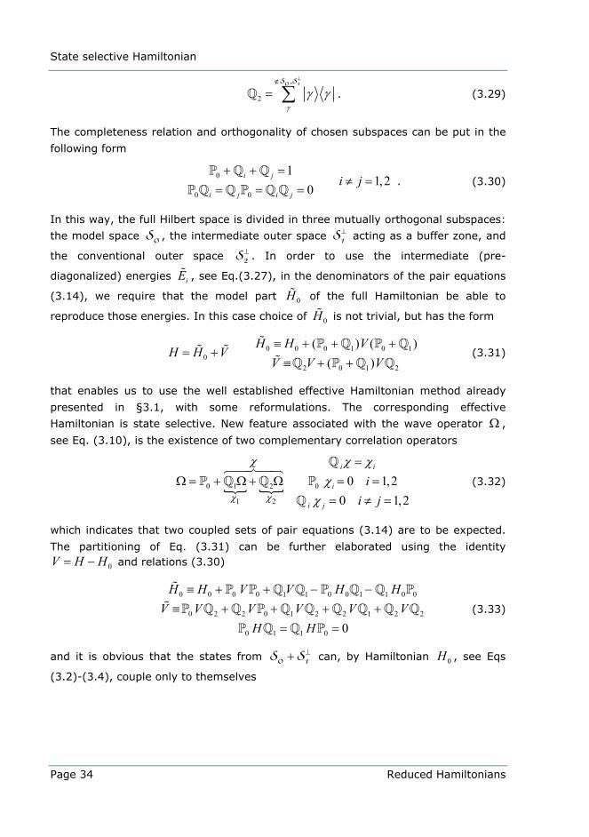
State selective Hamiltonian
Page 34 Reduced Hamiltonians
,
2γ
γ γ⊥∉
= ∑ 0 1S S
Q . (3.29)
The completeness relation and orthogonality of chosen subspaces can be put in the
following form
0
0 0
11,2
0i j
i j i ji j
+ + =≠ =
= = =P Q Q
P Q Q P Q Q . (3.30)
In this way, the full Hilbert space is divided in three mutually orthogonal subspaces:
the model space 0S , the intermediate outer space ⊥1S acting as a buffer zone, and
the conventional outer space ⊥2S . In order to use the intermediate (pre-
diagonalized) energies iE , see Eq.(3.27), in the denominators of the pair equations
(3.14), we require that the model part 0H of the full Hamiltonian be able to
reproduce those energies. In this case choice of 0H is not trivial, but has the form
0 0 0 1 0 10
2 0 1 2
( ) ( )( )
H H VH H V
V V V≡ + + +
= +≡ + +
P Q P QQ P Q Q
(3.31)
that enables us to use the well established effective Hamiltonian method already
presented in §3.1, with some reformulations. The corresponding effective
Hamiltonian is state selective. New feature associated with the wave operator Ω ,
see Eq. (3.10), is the existence of two complementary correlation operators
0 1 2 0
1 2
0 1,20 1,2
i i
i
i j
ii jχ χ
χ χ χχ
χ
=Ω = + Ω + Ω = =
= ≠ =
QP Q Q P
Q (3.32)
which indicates that two coupled sets of pair equations (3.14) are to be expected.
The partitioning of Eq. (3.31) can be further elaborated using the identity
0V H H= − and relations (3.30)
0 0 0 0 1 1 0 0 1 1 0 0
0 2 2 0 1 2 2 1 2 2
0 1 1 0 0
H H V V H HV V V V V V
H H
≡ + + − −≡ + + + +
= =
P P Q Q P Q Q PP Q Q P Q Q Q Q Q Q
P Q Q P (3.33)
and it is obvious that the states from ⊥+ 0 1S S can, by Hamiltonian 0H , see Eqs
(3.2)-(3.4), couple only to themselves
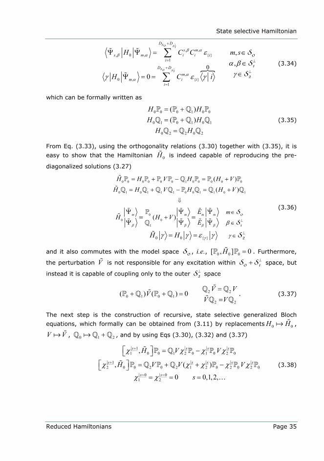
State selective Hamiltonian
Reduced Hamiltonians Page 35
, ,, 0 ,
1
,0 ,
1
0
,,
0
D Ds m
s m i i ii
D Dm
m i ii
H C C m s
H C i
β αβ α
αα
εα β
γγ ε γ
⊥
⊥
+
= ⊥
+⊥
=
Ψ Ψ = ∈∈
∈Ψ = =
∑
∑
S 0 S 1
S 0 S 1
0
1
2
S
S
S
(3.34)
which can be formally written as
0 0 0 1 0 0
0 1 0 1 0 1
0 2 2 0 2
( )( )
H HH H
H H
= += +
=
P P Q PQ P Q Q
Q Q Q (3.35)
From Eq. (3.33), using the orthogonality relations (3.30) together with (3.35), it is
easy to show that the Hamiltonian 0H is indeed capable of reproducing the pre-
diagonalized solutions (3.27)
0 0 0 0 0 0 1 0 0 0 0 0
0 1 0 1 1 1 0 0 1 1 0 1
00 0
1
0 0
( )
( )
( )m m m m m
H H V H H V
H H V H H V
EH H V
E
H Hβ β β β
γ
β
γγ γ ε γ
⊥
⊥
⇓
∈
∈
∈
= + − = +
= + − = +
Ψ Ψ Ψ+
Ψ Ψ Ψ= =
= =
0
1
2
S
S
S
P P P P Q P P PQ Q Q Q P Q Q Q
PQ
(3.36)
and it also commutes with the model space 0S , i.e., 0 0 0[ , ] 0H =P P . Furthermore,
the perturbation V is not responsible for any excitation within ⊥+ 0 1S S space, but
instead it is capable of coupling only to the outer ⊥2S space
2 20 1 0 1
2 2
( ) ( ) 0V V
VV V
=+ + =
=Q QP Q P QQ Q
. (3.37)
The next step is the construction of recursive, state selective generalized Bloch
equations, which formally can be obtained from (3.11) by replacements 0 0H H ,
V V , 0 1 2+Q Q Q , and by using Eqs (3.30), (3.32) and (3.37)
11 0 0 1 2 0 1 0 2 0
12 0 0 2 0 2 1 2 0 2 0 2 0
0 01 2
,
, ( )
0 0,1,2,
s s s s
s s s s s
s s
H V V
H V V V
s
χ χ χ χ
χ χ χ χ χ
χ χ
+
+
= =
⎡ ⎤ = −⎣ ⎦⎡ ⎤ = + + −⎣ ⎦
= = = …
P Q P P P
P Q P Q P P P (3.38)
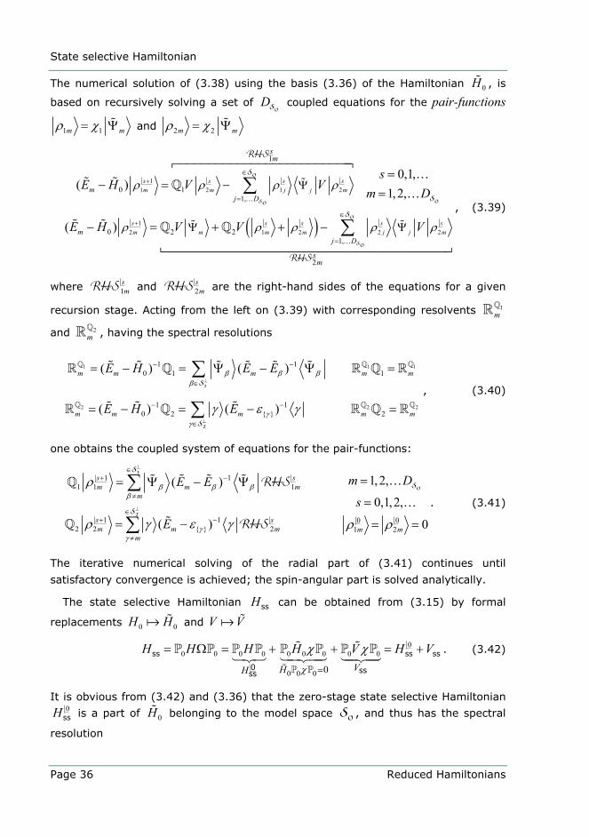
State selective Hamiltonian
Page 36 Reduced Hamiltonians
The numerical solution of (3.38) using the basis (3.36) of the Hamiltonian 0H , is
based on recursively solving a set of D 0S coupled equations for the pair-functions
1 1m mρ χ= Ψ and 2 2m mρ χ= Ψ
( )
11 2 1 2
12 1 2 2 2
0 11,
0 2 21,
1
2
0,1,( )
1,2,
( )
s s s sm m j j m
s s s s sm m m m j j m
mj D
mj D
sm
sm
sE H V V
m D
E H V V V
ρ ρ ρ ρ
ρ ρ ρ ρ ρ
+
+
∈
=
∈
=
Ψ
Ψ Ψ
=− = −
=
− = + + −
∑
∑
0
0S 0
0
S 0
S
S
S
…
…
……
Q
Q Q
RHS
RHS
, (3.39)
where 1smRHS and 2
smRHS are the right-hand sides of the equations for a given
recursion stage. Acting from the left on (3.39) with corresponding resolvents 1mQR
and 2mQR , having the spectral resolutions
1 1 1
2 2 2
1 10 1 1
1 10 2 2
( ) ( )
( ) ( )
m m m m m
m m m m m
E H E E
E H E
β β ββ
γγ
γ ε γ
⊥
⊥
− −
∈
− −
∈
= − = Ψ − Ψ =
= − = − =
∑
∑ 1
2
S
S
Q Q Q
Q Q Q
R Q R Q R
R Q R Q R, (3.40)
one obtains the coupled system of equations for the pair-functions:
1 11 1 1
1 1 0 02 2 2 1 2
1,2,( )0,1,2,
( ) 0
s sm m m
m
s sm m m m m
m
m DE Es
E
β β ββ
γγ
ρ
ρ γ ε γ ρ ρ
⊥
⊥
∈+ −
≠
∈+ −
≠
== Ψ − Ψ
=
= − = =
∑
∑
1
0
2
S
S
S
…
…Q
Q
RHS
RHS
. (3.41)
The iterative numerical solving of the radial part of (3.41) continues until
satisfactory convergence is achieved; the spin-angular part is solved analytically.
The state selective Hamiltonian ssH can be obtained from (3.15) by formal
replacements 0 0H H and V V
00 0 0 0 0 0 0 0 0
0 0 0 0
ss ss ss
0 ssssVHH
H H H H V H Vχ
χ χ=
= Ω = + + = +P P
P P P P P P P P . (3.42)
It is obvious from (3.42) and (3.36) that the zero-stage state selective Hamiltonian 0
ssH is a part of 0H belonging to the model space 0S , and thus has the spectral
resolution
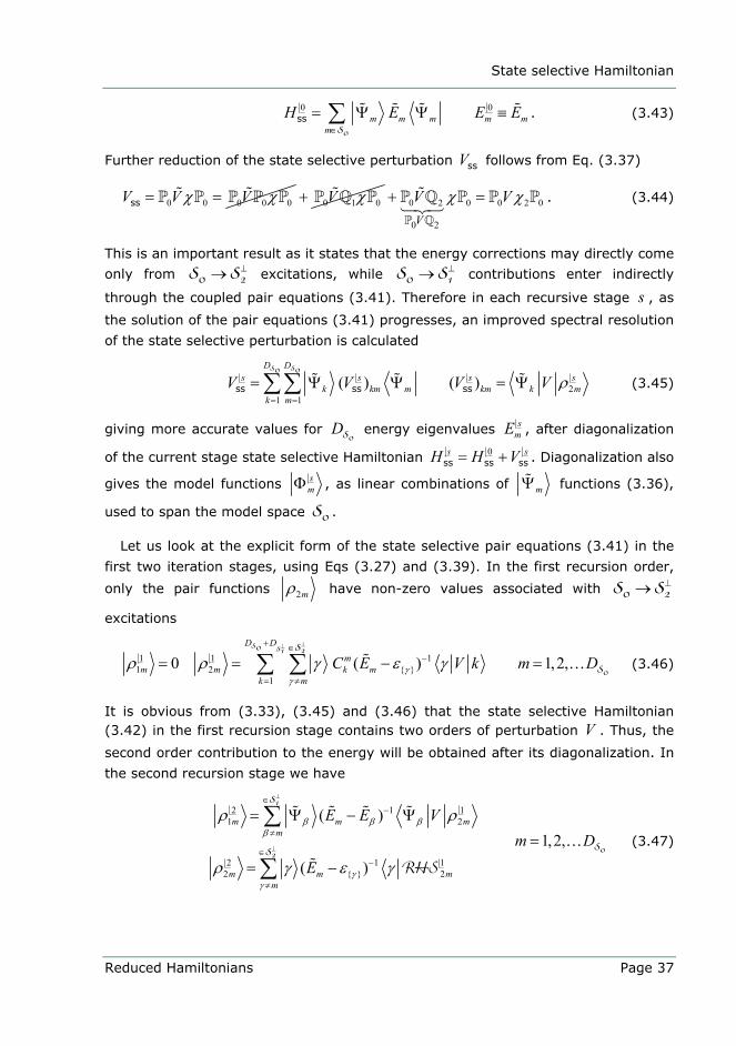
State selective Hamiltonian
Reduced Hamiltonians Page 37
0 0ss m m m m m
mH E E E
∈
= Ψ Ψ ≡∑ 0S
. (3.43)
Further reduction of the state selective perturbation ssV follows from Eq. (3.37)
0 0 0 0 0ssV V Vχ χ= =P P P P P 0 1 0V χ+ P Q P 0 2 0 0 2 0
0 2V
V Vχ χ+ =P Q
P Q P P P . (3.44)
This is an important result as it states that the energy corrections may directly come
only from ⊥→0 2S S excitations, while ⊥→0 1S S contributions enter indirectly
through the coupled pair equations (3.41). Therefore in each recursive stage s , as
the solution of the pair equations (3.41) progresses, an improved spectral resolution
of the state selective perturbation is calculated
21 1
( ) ( )ss ss ss
D Ds s s s
k km m km k mk m
V V V V ρ= =
= Ψ Ψ = Ψ∑ ∑S S 0 0
(3.45)
giving more accurate values for D0S energy eigenvalues s
mE , after diagonalization
of the current stage state selective Hamiltonian 0ss ss sss sH H V= + . Diagonalization also
gives the model functions smΦ , as linear combinations of mΨ functions (3.36),
used to span the model space 0S .
Let us look at the explicit form of the state selective pair equations (3.41) in the
first two iteration stages, using Eqs (3.27) and (3.39). In the first recursion order,
only the pair functions 2mρ have non-zero values associated with ⊥→ 0 2S S
excitations
1 1 11 2
1
0 ( ) 1,2,D D
mm m k m
k m
C E V k m Dγγ
ρ ρ γ ε γ⊥⊥+ ∈
−
= ≠
= = − =∑ ∑S 0 S 1 2
0
S
S… (3.46)
It is obvious from (3.33), (3.45) and (3.46) that the state selective Hamiltonian (3.42) in the first recursion stage contains two orders of perturbation V . Thus, the
second order contribution to the energy will be obtained after its diagonalization. In
the second recursion stage we have
2 1 11 2
2 1 12 2
( )1,2,
( )
m m mm
m m mm
E E Vm D
E
β β ββ
γγ
ρ ρ
ρ γ ε γ
⊥
⊥
∈−
≠
∈−
≠
= Ψ − Ψ
=
= −
∑
∑
1
0 2
S
SS…
RHS
(3.47)
State selective Hamiltonian
Page 38 Reduced Hamiltonians
where 12mRHS do not contain any contributions from 1mρ , and include up to three
orders of the perturbation V . This gives the state selective Hamiltonian with up to
four orders of perturbation. In the third recursive stage, for the first time 21mρ
enter in 22mRHS , contributing to the state selective Hamiltonian as terms
proportional to the fourth order of the perturbation V . This is consistent with
findings of Malrieu et al [58], that the excitations to intermediate space → M IS S
come in fourth order of the perturbative expansion of Eq. (3.23).
In the following, the efficiency of our approach will be illustrated on some doubly
excited states of helium, where previous accurate theoretical studies exist, see
Paper III. In order to do so, some introduction into the procedure of obtaining the
non-relativistic one-electron orbitals (3.2) is necessary.
Dragan Nikolié Page 39
Chapter 4 Numerical implementations
Although many-body problems are encountered in numerous areas of physics and
chemistry, the atomic many-body problem plays an important role for testing new
theoretical approaches. This is mainly because the two-body Coulomb interaction is
well understood. Furthermore, the existence of atomic systems with up to a hundred
electrons enables to test the scalability of theoretical models.
The interpreting power of any atomic many-body theory is seriously questioned
by ever-increasing capability of experiments to observe more and more details. In
return, the access to reliable theoretical predictions enables the planning and
development of new complex experimental techniques. Since the atoms are
constituents of larger systems like molecules, clusters and solids, any progress in
the calculation of the properties of atoms may indirectly influence the developments
in the other fields of science.
This chapter demonstrates both our ability to interpret the recombination of the
lithium-like ions in the storage ring experiments, and to contribute to the
development of new methods.
4.1 Non-relativistic framework
As mentioned earlier, see Eqs (3.2) and (3.3), we want to use coupled
eigenfunctions of the one-electron Hamiltonian to study electron-electron correlation in doubly excited states. The foundation of our numerical approach to doubly excited states is laid by Salomonson and Öster [66, 67] in the non-relativistic as well as the
relativistic framework. At this point, we restrict our selves to the non-relativistic
approach, aiming for some of the doubly excited states in the helium atom, coupled to a specific 2 1S Lπ+ symmetry. The helium atom, with both electrons excited, represents
an important test case for electron correlations in atomic systems, ever since the experiment by Madden and Codling [20]. They revealed that correlation plays a
Non-relativistic framework
Page 40 Numerical implementations
primary role in the formation of collective states of the electron pair. The knowledge
of the electron-electron correlation in two-electron atoms rapidly grew with the development of numerous computational techniques, see e.g. the reviews of Fano
[68], Buckman and Clark [69], Lin [70], Aymar et al [71] and Tanner et al [72].
4.1.1 One-electron spectrum
Confining the atom to a spherical box, Salomonson and Öster [66] converted the
radial one-electron Schrödinger equation
2 2
2 20
0
( 1) ( ) ( ) ( )2 e
r
d eV r P r P rm dr r
h
ε⎡ ⎤⎛ ⎞+− − + =⎢ ⎥⎜ ⎟
⎝ ⎠⎣ ⎦ , (4.1)
into a symmetric eigenvalue matrix equation
( )D B ε+ =P P , (4.2)
using the seven-point finite difference scheme for the second derivative in Eq. (4.1); D is a diagonal p pN N× matrix, with pN being the number of lattice points; if
( )V r is a local potential, B is a symmetric band matrix. The vector P has for its
pN elements the values of eigenfunctions ( ) ( )P x rP r= at the discretized
equidistant logarithmic mesh of the radial coordinate lnx r= . When diagonalized,
the symmetric Hermitian ( )D B+ matrix gives pN -orthogonal basis set orbitals
(complete on the chosen grid) and their corresponding eigenvalues for each partial-wave component . The radius of the spherical box, maxr , is chosen in a way not to
affect the states of interest when the boundary condition max( ) 0P r r≥ = is enforced.
One-electron orbitals bound by the nuclear potential will have negative eigenvalues,
and those bound by the spherical box will have positive eigenvalues, representing a
discretized continuum. In contrast to the lowest ones, the highest negative
eigenvalues, close to the threshold, will not be truly hydrogen-like, since they are
affected by the cavity. In order to illustrate the size of the basis set, let us assume that the discretized grid for the radial coordinate has 211pN = points, and the
partial wave expansion includes components up to max 10= . The number of one-
electron orbitals will then be
max
max0 1
( 1) 2321pN
pj
N+
= = +
= + =∑ ∑ . (4.3)
We use these orbitals to define the solutions (3.3) of the two-electron unperturbed
Hamiltonian, and to construct correlated wave functions to all orders in the iterative
expansion of the residual electron-electron interaction by solving the pair equations
Non-relativistic framework
Numerical implementations Page 41
(3.41). When these correlated wave functions describe the autoionizing doubly
excited states, which are embedded in (and thus coupled to) the continuum, one
has to deal with poles in the energy denominators of Eq. (3.41), coming from
discretized continuum states with energies mEγε ≈ . The complex rotation method
offers an elegant way to move discretized continuum energies away from the real
energy axis, thus effectively removing singularities. This method is nowadays a
standard approach to study various atomic systems with states coupled to the
continuum. Here, only the main physical ideas of complex scaling will be outlined, for the original mathematical background, see Balslev and Combes [73]. The simplicity
and efficiency of the complex scaling method enabled its wide usage: from the first application to wave problems in meteorology Tannhauser and Moiseyev [74], to the
resonances of helium in a DC field Chung et al [75]. For a nice review on this subject
see Moiseyev [76].
The complex scaling method extends the use of bound state techniques to autoionizing states. It is achieved, see Moiseyev et al [77], by complex scaling of the
radial ( )
exp( )R
r r iθ
θ→ and consequently momentum ( )
exp( )R
p p iθ
θ−
→ − coordinates,
providing the rotated Hamiltonian ( )R
H Hθ
θ→ with the following properties:
The bound state energies of Hθ remain the same as those of H .
The positions of thresholds thE are independent of θ , but associated
segments of continua are rotated around them by an angle 2θ− .
The Hermicity of Hθ is destroyed, but its complex eigenvalues mE θ
satisfying 2 ( )m thArg E Eθθ− ≤ − can be associated with resonance
energies of H , see Simon [78], as / 2m m mE E iθ = − Γ .
Non-integrable continuum wave functions are rotated in the Hilbert space into square integrable eigenfunctions of Hθ
Therefore, Eq. (4.1) will under complex rotation transform into, see Lindroth [43],
2 2
22 2
0
0
( 1) ( ) ( ) ( )2
e e e ei i i i
e
r
d eV r P r P rm dr r
h
θ θ θ θ
θ
ε−⎡ ⎤⎛ ⎞+− − + =⎢ ⎥⎜ ⎟
⎝ ⎠⎣ ⎦ (4.4)
whose discretization using the method of Salomonson and Öster [66] provides one-electron spectra, with the 0= component as illustrated in Figure 9 for several
rotational angles.
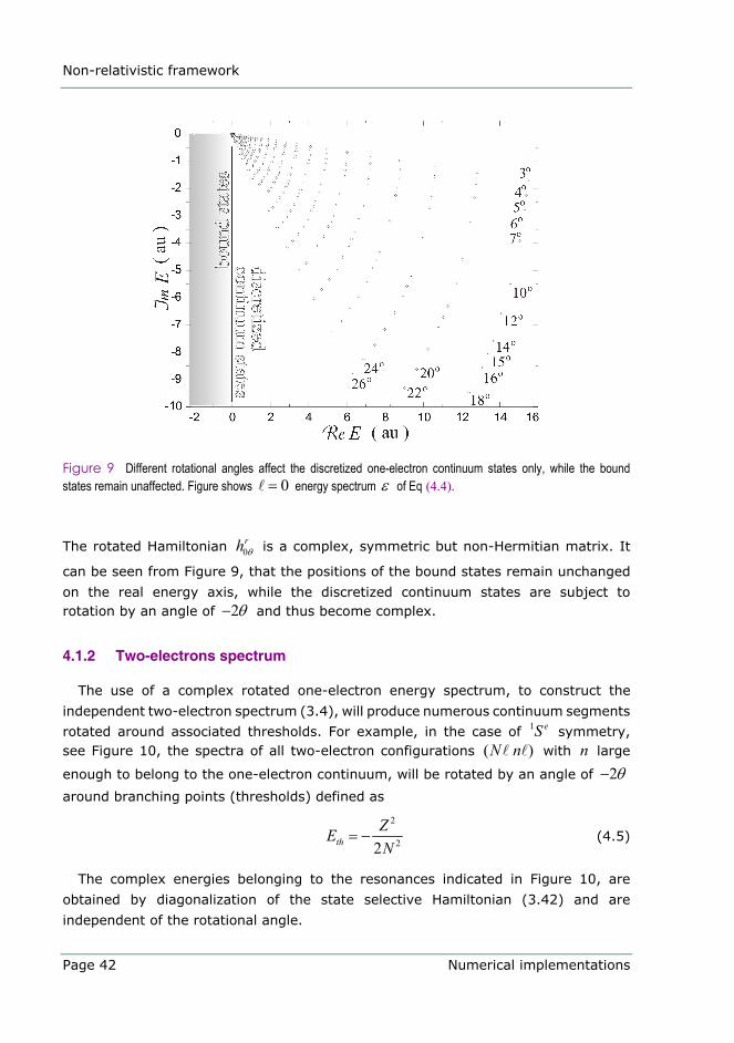
Non-relativistic framework
Page 42 Numerical implementations
Figure 9 Different rotational angles affect the discretized one-electron continuum states only, while the bound states remain unaffected. Figure shows 0= energy spectrum ε of Eq (4.4).
The rotated Hamiltonian 0rh θ is a complex, symmetric but non-Hermitian matrix. It
can be seen from Figure 9, that the positions of the bound states remain unchanged
on the real energy axis, while the discretized continuum states are subject to rotation by an angle of 2θ− and thus become complex.
4.1.2 Two-electrons spectrum
The use of a complex rotated one-electron energy spectrum, to construct the
independent two-electron spectrum (3.4), will produce numerous continuum segments
rotated around associated thresholds. For example, in the case of 1 eS symmetry, see Figure 10, the spectra of all two-electron configurations ( )N n with n large
enough to belong to the one-electron continuum, will be rotated by an angle of 2θ−
around branching points (thresholds) defined as
2
22thZEN
= − (4.5)
The complex energies belonging to the resonances indicated in Figure 10, are
obtained by diagonalization of the state selective Hamiltonian (3.42) and are
independent of the rotational angle.
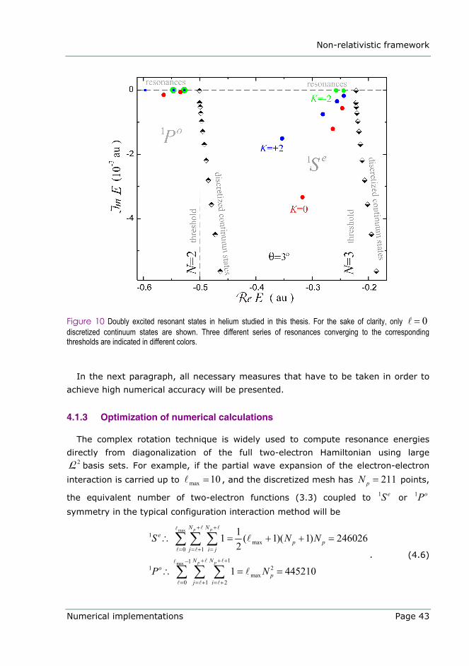
Non-relativistic framework
Numerical implementations Page 43
Figure 10 Doubly excited resonant states in helium studied in this thesis. For the sake of clarity, only 0= discretized continuum states are shown. Three different series of resonances converging to the corresponding thresholds are indicated in different colors.
In the next paragraph, all necessary measures that have to be taken in order to
achieve high numerical accuracy will be presented.
4.1.3 Optimization of numerical calculations
The complex rotation technique is widely used to compute resonance energies
directly from diagonalization of the full two-electron Hamiltonian using large 2L basis sets. For example, if the partial wave expansion of the electron-electron
interaction is carried up to max 10= , and the discretized mesh has 211pN = points,
the equivalent number of two-electron functions (3.3) coupled to 1 eS or 1 oP
symmetry in the typical configuration interaction method will be
max
max
1max
0 1
111 2
max0 1 2
11 ( 1)( 1) 2460262
1 445210
p p
p p
N Ne
p pj i j
N No
pj i
S N N
P N
+ +
= = + =
+ + +−
= = + = +
∴ = + + =
∴ = =
∑ ∑ ∑
∑ ∑ ∑. (4.6)
Non-relativistic framework
Page 44 Numerical implementations
It is obvious from Eq.(4.6) that the dimension of the matrix to be diagonalized
scales as 2 2max( )pN∼ . However, with the use of the effective Hamiltonian method, only
part of the spectrum is calculated. For example, in the case of 1 eS symmetry, the
computing resources are dedicated only to the storage of a max( 1) pN+ complex
scaled one-electron orbitals (4.3), with the max( 1)D+0S pair functions (3.41), each
2pN large and a matrix of dimension D D×
0 0S S has to be diagonalized.
It is obvious, from the first iteration order (3.46) of the pair equations (3.41),
that the numerical accuracy of the pair functions depends on our ability to calculate
the matrix elements V cγ , that is (see Eq. (3.3))
( , ) ( , )1 2 1 2
1 2 1 2 2 1
2(1 ( 1) )(1/ 2)
( 1)
c cc
cc c c cLS LS LS
V c
V
γ γγ δ δϕ ϕ
ϕγ γ
γ
φ φ φ φ φ φ
+ ++= + − ×
⎡ ⎤+ −⎣ ⎦ (4.7)
In the case when perturbation 112V r−= represents the Coulomb electron-electron
repulsion (in atomic units), its partial wave expansion (see e.g. p. 94 of Lindgren and Morrison [40]) leads to the following useful result
max
1 2 1 2 1 2 1 2
min
1 1 2 2 1 1 2 2min 1 1 2 2max
112 1 2 1 2
MaxMin
max
( , ) ( , )
| | ,
0,1,
kk k
c c c cLS LSk k
c c c cc c
c
r L c c
Lk
γ γ γ γ
γ γ γ γγ γ
γ
φ φ φ φ γ γ−
=
=
− ≤ ≤ +=
=
∑
∓ ∓…
A R
(4.8)
where the angular parts kA are solved analytically since they consist of a phase factor, a 6 j symbol and two reduced matrix elements of the C tensor (see p. 45 of
Ref [40]). The radial parts kR are the Slater integrals
1 2 1 21 2 1 2 1 2 1 2 1 21( , ) ( ) ( ) ( ) ( )
kk
c ck
rc c P r P r P r P r dr drrγ γγ γ <
+>
= ∫∫R , (4.9)
with ( )P r being the radial one-particle solutions of (4.4), and Min1 2Max , r r r<
>= having
a cusp for 1 2r r= . The existence of the cusp, especially for large angular momentum
k transferred along the Coulomb interaction, is the main source of error if the
Slater integrals are to be evaluated to high accuracy. The quadrature of (4.9)
depends on the lattice spacing h , and the initial 6h accuracy of the seven-point
finite difference formula
2 63 3 2 2 1 1( 216( ) 135( ) 245 ) / 90 ( )k k k k k k k kP P P P P P P P h h− + − + − +′′= + − + + + − +O (4.10)
is reduced to 2h level by the presence of the cusp. In order to improve the
integration over the cusp, Salomonson and Öster [66] introduced a weighting of the
Non-relativistic framework
Numerical implementations Page 45
points close to it. With this weighting the remaining error is 4( )hO . In this thesis,
similar to Ref. [66], a systematic investigation of the lattice spacing h for doubly
excited states in helium is performed. For that purpose, the lattice range is set to
7 6.5min max/ , / , 2r e Z r e Z Z− += = = , (4.11)
and discretized in three different meshes corresponding to 151,191,211pN = points.
The following dependence of the converged energies is assumed, see [66],
4 5 64 5( ) (0) ( )E h E a h a h h= + + +O , (4.12)
where the coefficients are obtained by fitting the converged energies, for a fixed maximal partial wave component and complex scaling angle θ . What remains is
the 6( )hO energy error, which is less than 123 10 au−⋅ for all investigated doubly
excited states. From this point on, unless indicated differently, it is assumed that
the energies are optimized with respect to the lattice spacing, in order to
concentrate on the other accuracy limiting factors. Keeping the complex scaling
angle fixed, we now proceed to investigate the convergence rate of our calculations
with respect to the partial wave expansion of the electron-electron interaction. For that purpose, it is advisable to use the concept of forward differences. If ( )E
represents the converged complex energy of a certain doubly excited state, for a fixed angle θ and a maximal orbital quantum number one electron orbitals are
allowed to posses, in accordance to (4.8), the forward difference is defined as
( ) ( 1) ( )E E E∆ = + − . (4.13)
It is related to the contribution of the next term in the multipole expansion of the electron-electron interaction, with an ideal ( ) 0E∆ ∞ → tendency. However, in the
numerical implementations a cut-off of the partial wave expansion is set to a certain value of max= , which is max 10= in this work. To estimate the contribution of the
terms higher than max , an extrapolation procedure has to be used. The Aitken’s 2δ
process, see for example [79], is used in Papers II and I, but in the Paper III, the extrapolation scheme of Ref. [66] (based on Carroll et al [80]) is employed; the
forward differences (4.13) are fitted to the following expression
2
0 0( ) ( , , ) ( )n
n
n
E E n D ξξ
ξ
+−
=
∆ ∆ = +∑ (4.14)
where the parameter 0 is found to be close to 0.5 , and set to that value further on.
The coefficients nDξ are obtained for different values of parameter 2,3,4n = of which
4n = is chosen, giving the minimal value for 2χ -merit function. The applicability of
the extrapolation scheme given in Ref. [66] is therefore confirmed also for doubly
excited states investigated here. Since the forward differences obey the rule
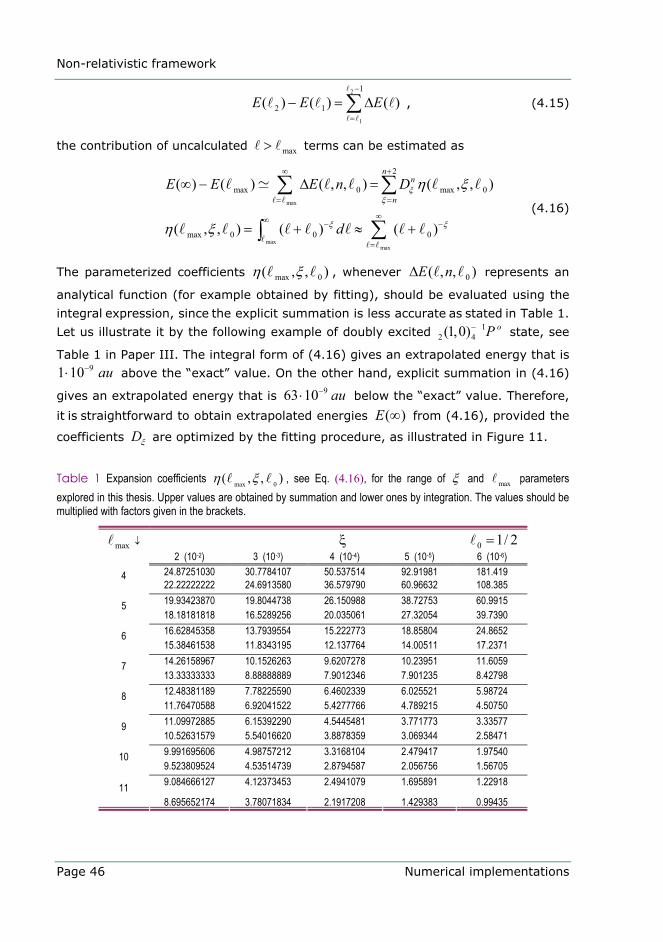
Non-relativistic framework
Page 46 Numerical implementations
2
1
1
2 1( ) ( ) ( )E E E−
=
− = ∆∑ , (4.15)
the contribution of uncalculated max> terms can be estimated as
max
maxmax
2
max 0 max 0
max 0 0 0
( ) ( ) ( , , ) ( , , )
( , , ) ( ) ( )
nn
nE E E n D
d
ξξ
ξ ξ
η ξ
η ξ
∞ +
= =
∞∞ − −
=
∞ − ∆ =
= + ≈ +
∑ ∑
∑∫ (4.16)
The parameterized coefficients max 0( , , )η ξ , whenever 0( , , )E n∆ represents an
analytical function (for example obtained by fitting), should be evaluated using the
integral expression, since the explicit summation is less accurate as stated in Table 1.
Let us illustrate it by the following example of doubly excited 12 4(1,0) oP− state, see
Table 1 in Paper III. The integral form of (4.16) gives an extrapolated energy that is 91 10 au−⋅ above the “exact” value. On the other hand, explicit summation in (4.16)
gives an extrapolated energy that is 963 10 au−⋅ below the “exact” value. Therefore,
it is straightforward to obtain extrapolated energies ( )E ∞ from (4.16), provided the
coefficients Dξ are optimized by the fitting procedure, as illustrated in Figure 11.
Table 1 Expansion coefficients max 0( , , )η ξ , see Eq. (4.16), for the range of ξ and max parameters explored in this thesis. Upper values are obtained by summation and lower ones by integration. The values should be multiplied with factors given in the brackets.
ξ 0 1/ 2= max ↓ 2 (10-2) 3 (10-3) 4 (10-4) 5 (10-5) 6 (10-6)
24.87251030 30.7784107 50.537514 92.91981 181.419 4 22.22222222 24.6913580 36.579790 60.96632 108.385 19.93423870 19.8044738 26.150988 38.72753 60.9915 5 18.18181818 16.5289256 20.035061 27.32054 39.7390 16.62845358 13.7939554 15.222773 18.85804 24.8652 6 15.38461538 11.8343195 12.137764 14.00511 17.2371 14.26158967 10.1526263 9.6207278 10.23951 11.6059 7 13.33333333 8.88888889 7.9012346 7.901235 8.42798 12.48381189 7.78225590 6.4602339 6.025521 5.98724 8 11.76470588 6.92041522 5.4277766 4.789215 4.50750 11.09972885 6.15392290 4.5445481 3.771773 3.33577 9 10.52631579 5.54016620 3.8878359 3.069344 2.58471 9.991695606 4.98757212 3.3168104 2.479417 1.97540 10 9.523809524 4.53514739 2.8794587 2.056756 1.56705 9.084666127 4.12373453 2.4941079 1.695891 1.22918 11 8.695652174 3.78071834 2.1917208 1.429383 0.99435
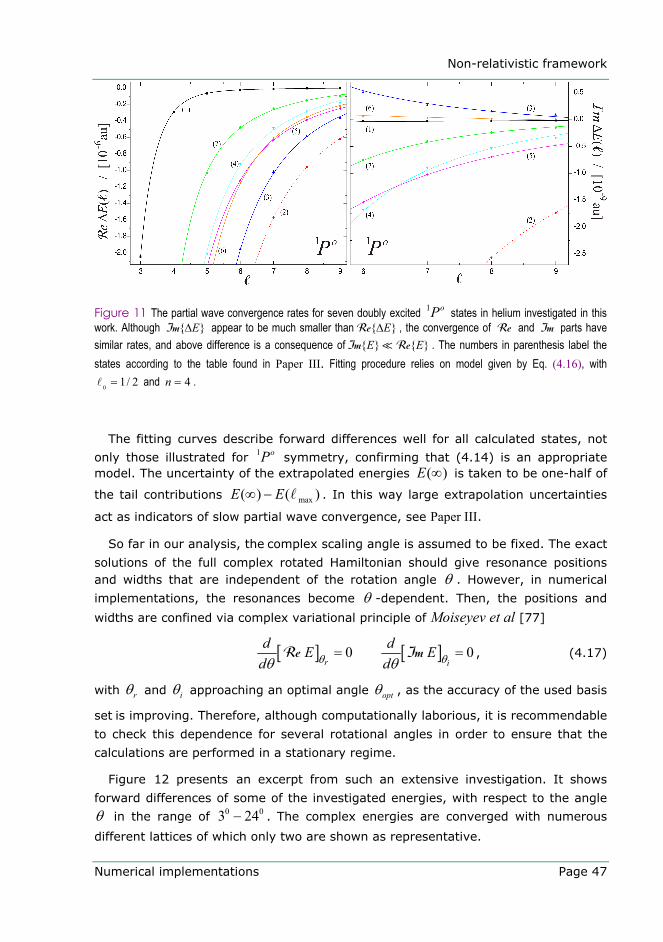
Non-relativistic framework
Numerical implementations Page 47
Figure 11 The partial wave convergence rates for seven doubly excited 1 oP states in helium investigated in this work. Although E∆Im appear to be much smaller than E∆Re , the convergence of Re and Im parts have similar rates, and above difference is a consequence of E EIm Re . The numbers in parenthesis label the states according to the table found in Paper III. Fitting procedure relies on model given by Eq. (4.16), with
0 1/ 2= and 4n = .
The fitting curves describe forward differences well for all calculated states, not
only those illustrated for 1 oP symmetry, confirming that (4.14) is an appropriate model. The uncertainty of the extrapolated energies ( )E ∞ is taken to be one-half of
the tail contributions max( ) ( )E E∞ − . In this way large extrapolation uncertainties
act as indicators of slow partial wave convergence, see Paper III.
So far in our analysis, the complex scaling angle is assumed to be fixed. The exact
solutions of the full complex rotated Hamiltonian should give resonance positions and widths that are independent of the rotation angle θ . However, in numerical
implementations, the resonances become θ -dependent. Then, the positions and
widths are confined via complex variational principle of Moiseyev et al [77]
[ ] [ ]0 0r i
d dE Ed dθ θθ θ
= =Re Im , (4.17)
with rθ and iθ approaching an optimal angle optθ , as the accuracy of the used basis
set is improving. Therefore, although computationally laborious, it is recommendable
to check this dependence for several rotational angles in order to ensure that the
calculations are performed in a stationary regime.
Figure 12 presents an excerpt from such an extensive investigation. It shows
forward differences of some of the investigated energies, with respect to the angle
θ in the range of 0 03 24− . The complex energies are converged with numerous
different lattices of which only two are shown as representative.
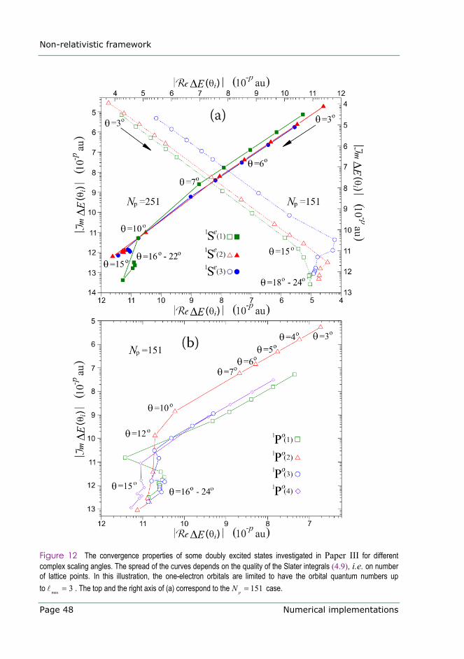
Non-relativistic framework
Page 48 Numerical implementations
Figure 12 The convergence properties of some doubly excited states investigated in Paper III for different complex scaling angles. The spread of the curves depends on the quality of the Slater integrals (4.9), i.e. on number of lattice points. In this illustration, the one-electron orbitals are limited to have the orbital quantum numbers up to max 3= . The top and the right axis of (a) correspond to the 151pN = case.
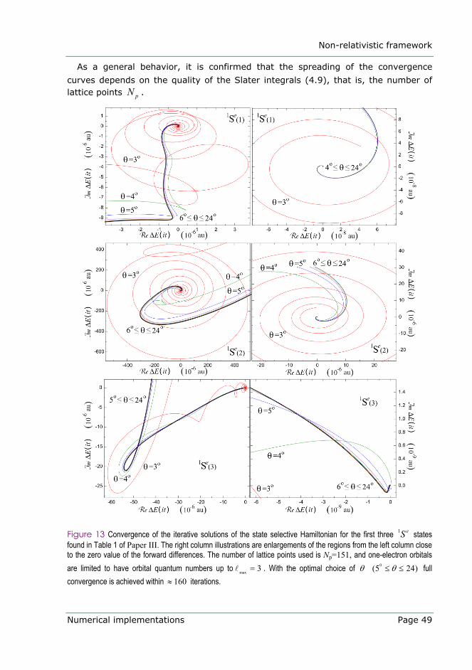
Non-relativistic framework
Numerical implementations Page 49
As a general behavior, it is confirmed that the spreading of the convergence
curves depends on the quality of the Slater integrals (4.9), that is, the number of lattice points pN .
Figure 13 Convergence of the iterative solutions of the state selective Hamiltonian for the first three 1 eS states found in Table 1 of Paper III. The right column illustrations are enlargements of the regions from the left column close to the zero value of the forward differences. The number of lattice points used is Np=151, and one-electron orbitals are limited to have orbital quantum numbers up to max 3= . With the optimal choice of θ 0(5 24)θ≤ ≤ full convergence is achieved within 160≈ iterations.
Li-like and Be-like ions in a relativistic framework
Page 50 Numerical implementations
For example, if 251pN = is used, the improvement of the collective convergence
rate is noticeable. However, the breaking of the collective convergence is found for
151pN = , where some states converge slower for rotational angles less than 015 .
In this example, in order to reach 12 significant digits for the resonance widths and 11 for the positions, the complex scaling angle has to be larger than 015 . This
conclusion remains for the values of one electron angular momenta up to max 10= .
It is interesting that the other methods using the complex scaling, see for example
Chung et al [75], Elander et al [81], also report very stable results for 015θ ≥ . What
about rotational angles below 03θ = ? Theoretically, complex scaling angles 00.5θ ≥
are sufficient for uncovering all the doubly excited resonances we considered in helium.
In practice however, we were not able to achieve convergence for rotational
angles in the range of 0 00.5 2.5θ≤ ≤ within 200itN = iterations, although 150itN =
iterations are enough for 015θ = angle.
A closer inspection for 04θ < revealed that iterative solutions exhibit spiral patterns
in a wide range, one of which is illustrated in Figure 13 for 03θ = . The forward
differences are constructed out of energies obtained in each recursive stage of the
solution of the pair equations, see Eq. (3.41). If the convergence is met, these
differences for real and imaginary parts of the energies should tend to zero. The
path along which this tendency is fulfilled, however, depends not only on rotational angle θ , but also on the state of interest as Figure 13 demonstrates.
4.2 Li-like and Be-like ions in a relativistic framework
When dealing with atomic systems with more than two-electrons, the treatment of three and four electron excitations have to be considered, which leads naturally to the
coupled-cluster (CC) approach. Our aim is to obtain relativistic one-electron orbitals as
building blocks for the many-body perturbation theory formulated in the no-virtual-pair
open-shell CC scheme, see Lindgren [50], Lindgren and Morrison [40], Lindgren and Mukherjee [82]. The details concerning the formalism of second quantization in the
particle-hole formulation, and the normal order representation of the wave operator and the effective interaction can be found in Lindgren and Morrison [40]. Therefore,
I shall present here only a short description of the method. For a nice introduction to the coupled-cluster approach, the reader is referred to Bishop and Kümmel [83].
The wave operator Ω , defined in §3.1, is in the original closed-shell CC procedure
expressed in the form of exponential ansatz
2 31 12! 3!1eS S S SΩ ≡ = + + + +… (4.18)
The cluster operator S , in representation of the second quantization, has the form
Li-like and Be-like ions in a relativistic framework
Numerical implementations Page 51
† † †12
1 2singles: doubles:
j jlj i i j l k i ik
ij ijkl
S S
S a a a a a a= + +∑ ∑ … , (4.19)
where † ( )a a are creation (annihilation) operators, and the coefficients represent the
corresponding excitation amplitudes. The excitation refers to an operation of cluster
operator involving the same number of annihilations and creations, even if the same
orbital is involved in both processes. If an electron is annihilated and created in the same orbital, it is said to be passive. Therefore, it is possible to include one-body effects in the two-body operator by adding one passive electron. Graphically S is represented only by connected diagrams, which cannot be separated into two parts without breaking any orbital or interaction line. This condition is the consequence of the linked-
cluster theorem [50] and provides the size-consistency (the total energy should scale
linearly with the number of particles). In order to extend the closed-shell CC approach to open-shell systems with only minor modifications, the ordinary products in (4.18)
have to be replaced by normal products with respect to a certain reference state,
2 31 12! 3!1eS S S SΩ ≡ = + + + +… (4.20)
where curly brackets denote such products. Substituting (4.20) into the generalized Bloch equation (3.9), retaining only connected terms of (4.19) grouped into one-, two-
, … many-particle excitations, a set of self-consistent CC equations is obtained:
( )0 0 0 ,[ , ] 1,2,
connn n
nRHS
S H V V nχ= Ω − Ω = …Q P (4.21)
where the subscript n denotes that only n simultaneous excitations in the right-
hand side nRHS are considered. The coupled-cluster approach is a way of including as
many effects as possible within a given truncation scheme. For example, the coupled-cluster singles and doubles (CCSD) approximation is defined by retaining only the
single- and double-excitations in Eqs (4.20) and (4.21). However, the most
important three and four body effects are also taken into account in the wave
operator (4.20) through the 2S term. Therefore, the wave operator constructed using
(4.20) and (4.21), usually gives results in which 95-98% of the electron correlation is included [84]. In order to perform any numerical treatment of coupled-cluster
equations, each operator entering in (4.21) has to be uniquely specified (regarding the elementary excitations it provides) by means of the normal-ordered second-
quantization.
4.2.1 Computational method
The Coulomb repulsion among the electrons is usually too large to be taken as a whole, when forming the perturbation V . To improve the convergence rate, it is
Li-like and Be-like ions in a relativistic framework
Page 52 Numerical implementations
possible to introduce an additional single-electron potential ( )iu r , that ith electron
feels from the other electrons. In the independent particle model, it is customary to
assume that each electron in the atom moves independently of the other electrons,
but in an average field generated by the nucleus and the electrons. This average, a non-local spherically symmetric potential ( )u r , in our calculations represents the
Dirac-Fock-Breit potential from the closed 21s -core, and optionally a projected
potential of the form given in (3.26). Then Eq. (2.10) transforms to
2
0
( )( ) ( )( ) ( )
( ) 2
n n
n ne
dV r cf r f rdr rg r g rdc V r m c
dr r
κ κ
κ κ
κ
εκ
⎛ ⎞⎛ ⎞− −⎜ ⎟⎜ ⎟ ⎛ ⎞ ⎛ ⎞⎝ ⎠⎜ ⎟ =⎜ ⎟ ⎜ ⎟⎜ ⎟⎛ ⎞ ⎝ ⎠ ⎝ ⎠+ −⎜ ⎟⎜ ⎟⎝ ⎠⎝ ⎠
, (4.22)
with ( ) ( ) ( )nucV r V r u r= + . The nuclear size corrections are included in the potential
( )nucV r coming from the extended nucleus, described by the Thomas-Fermi model,
see Desclaux [85] and Johnson and Soff [86].
In order to solve (4.22) or (2.10), the method of Salomonson and Öster [67] is
used. The atom is confined into a spherical radial box, with the radial coordinate discretized into pN -points grid. The size of the box is carefully chosen not to affect
the bound states of interest, and a logarithmic lattice is used in order to represent
the wave function close to the nucleus. The cavity size effect can be estimated by
adding more points to the radial grid preserving the lattice spacing and monitoring
the disturbance of the eigenspectrum. Discretizing the coupled system of differential
equations (4.22) for the large and small components, it is reduced to a symmetric 2 2p pN N× matrix equation. When solved, a complete numerical set of ( pN positive
energy and pN negative energy) orthogonal radial eigenvectors are obtained.
This numerical basis set, consisting of the single-electron spinors (2.6) with the
radial part obtained from (4.22), is then used to construct the Slater determinants
α that will span the model space 0S . In contrast to (3.3), but in agreement with
the description in Lindgren and Morrison [40], these spanning determinants are not
coupled to a specific symmetry, and therefore are capable of giving the eigenspectrum of the effective Hamiltonian (3.15) for all symmetries of interest. The 1RHS of Eq.
(4.21), when acting on any spanning determinant α ∈ 0S from the model space, must
produce single excitations jiα
⊥∈ 0S outside the model space. Therefore, the single
excitation amplitudes from (4.19) can be calculated as
( )
,1 conn
jij
ii j
RHSα α
ε ε=
− , (4.23)
Li-like and Be-like ions in a relativistic framework
Numerical implementations Page 53
where the Slater determinant jiα is obtained from α by replacing the spinor
( )i rφ with ( )j rφ . It is thus possible to define single-excitation function ( )i rζ that
resembles the effects of 1S acting on any spanning determinant, by:
( )
,1( ) conn
j j ji i ij j
i i ij j i j
RHSr
α α α αζ α
ε ε α
⊥∈= =
− ∈∑ ∑ 0
0
S
S (4.24)
In a similar manner, the cluster equation for the operator 2S can be obtained (for
the details refer to [40] and [87]), where the resulting pair (double-excitation) function 1 2( , )ik r rρ , see (3.14), is given by:
( )2,
1 2( , ) conn
jl jl jlik ik ikjl jl
ik ik ikjl jl i j k l
RHSr r
α α α αρ α
ε ε ε ε α
⊥∈= =
− + − ∈∑ ∑ 0
0
S
S. (4.25)
A set of two coupled equations, formed of single- and double-excitations functions,
(4.24) and (4.25), is solved recursively order-by-order to self-consistency; the first-
order set of coupled equations is
( )
( )
,
2 ,
(1)
(1)1 2
1( )
( , )
conn
conn
j jji ij j
ii i ij j i j jl
ikjl jlik ikjl jl
ik ik ikjl jl i j k l
Vr
Vr r
α α α αζ αε ε
αα α α
αρ αε ε ε ε
⊥
⊥
∈= =−
∈
∈= =− + −
∑ ∑
∑ ∑
0
0
0
S
S
S
. (4.26)
The solutions of (4.26) are then used to evaluate RHS α of Eqs. (4.24) and (4.25),
to obtain the second-order set of coupled equations, and so on until convergence.
The no-virtual-pair approximation, see §2.2, is incorporated in the set of coupled
equations (4.24) and (4.25) by restricting the summation to electron states only,
both bound ( 202 0em c ε− < < ) and discretized continuum ( 0ε ≥ ) states.
As in the non-relativistic framework, see §4.1.1, in order to describe the
autoionizing doubly excited states, the hydrogen-like radial Dirac equation (4.22)
has to be complex rotated.
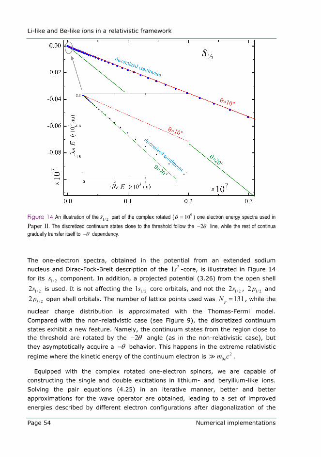
Li-like and Be-like ions in a relativistic framework
Page 54 Numerical implementations
Figure 14 An illustration of the 1/ 2s part of the complex rotated ( 010θ = ) one electron energy spectra used in Paper II. The discretized continuum states close to the threshold follow the 2θ− line, while the rest of continua gradually transfer itself to θ− dependency.
The one-electron spectra, obtained in the potential from an extended sodium
nucleus and Dirac-Fock-Breit description of the 21s -core, is illustrated in Figure 14
for its 1/ 2s component. In addition, a projected potential (3.26) from the open shell
1/ 22s is used. It is not affecting the 1/ 21s core orbitals, and not the 1/ 22s , 1/ 22 p and
3/ 22 p open shell orbitals. The number of lattice points used was 131pN = , while the
nuclear charge distribution is approximated with the Thomas-Fermi model.
Compared with the non-relativistic case (see Figure 9), the discretized continuum
states exhibit a new feature. Namely, the continuum states from the region close to the threshold are rotated by the 2θ− angle (as in the non-relativistic case), but
they asymptotically acquire a θ− behavior. This happens in the extreme relativistic
regime where the kinetic energy of the continuum electron is 20em c .
Equipped with the complex rotated one-electron spinors, we are capable of
constructing the single and double excitations in lithium- and beryllium-like ions.
Solving the pair equations (4.25) in an iterative manner, better and better
approximations for the wave operator are obtained, leading to a set of improved
energies described by different electron configurations after diagonalization of the
Li-like and Be-like ions in a relativistic framework
Numerical implementations Page 55
effective Hamiltonian (3.15). The details concerning the various aspects of the calculation of the lithium-like sodium ion can be found in Nikolić [39] and Paper II,
while those of the lithium-like beryllium ion are presented in Paper I. In the
following, only a short description of the standard procedure used to generate those
results will be outlined.
4.2.2 The lithium-like ions
According to the energy conservation law, given in the form of (1.4), the
knowledge of the precise placements of the recombination resonances depends heavily on our ability to: (1) accurately calculate the excitation energies 1,2E∆ in the
target lithium-like ion, and (2) to find the binding energy ( )b jE n of the captured
electron, with respect to the excited target ion, see Figure 2.
To obtain accurate values for 1,2E∆ , the Thomas-Fermi nuclear charge distribution is
adopted, after a series of calculations also involving the Point Charge and Uniform
Sphere models. In addition, different radial box sizes and meshes are tested. At this point, the Dirac-Fock energies of the 2 j orbitals in the averaged potential of the
nucleus and 1s2-core, with error bars corresponding to 1σ -confidence interval are
available. Further, we investigate the contribution of the Breit interaction (2.12)
when added to the instantaneous Coulomb electron-electron interaction, to form the
Dirac-Fock-Breit Hamiltonian. In addition, the mass polarization is calculated in
accordance with (2.14).
The dominating electron-electron correlation contribution comes in 2nd order of
the perturbation expansion, where the two-body perturbation is the sum of the
Coulomb and Breit interactions. The terms corresponding to the two Coulomb
interactions (C-C), as well as one Coulomb and one Breit interaction (C-B), are
separately presented in Table 1 of Paper I and Table 2 of Paper II. Depending on the
nature (core or valence) of the orbitals entering the one-body part of the
perturbation, further separation of the contributions into core-core and core-valence
is possible. In both cases (C-C and C-B), the partial-wave expansion of the Coulomb repulsion is carried out up to max 10= and extrapolated from there, using Aitken’s
2δ process [79]. Thus, the value for the 2nd order core-valence (C-B) contribution is
an extrapolated value from the partial wave expansion, identical to the (C-C) case. For light ions, the total 2nd order (C-B) contribution is often a few percent of the total
2nd order (C-C) counterpart, and the interaction within the core (core-core), has also a smaller influence on the binding energies of the 2 j orbitals than the core-
valence interaction. Higher-order correlation is calculated using the coupled-cluster
single- and double- (CCSD) excitation method mentioned in §4.2.1. When compared with the 2nd order results obtained by Johnson et al [88] good agreement is
Li-like and Be-like ions in a relativistic framework
Page 56 Numerical implementations
achieved. The small difference may come from the fact that in Ref. [88] partial wave expansion is carried out only up to max 8= and a Dirac-Fock basis set is used
instead. Summing up all the relevant contributions, one gets the Relativistic Many-
Body Perturbation Theory result in the CCSD scheme.
As the first step towards the inclusion of the radiative corrections, the largest
contributions (self-energy and vacuum polarization, see §2.5) for the hydrogen-like ions are taken from Johnson and Soff [86]. Then, the screening of the self-energy of the valence 2 j electrons, present in the non-hydrogenic ions, can be interpolated
using the recent results of Indelicato and Mohr [89], and possibly compared with
extrapolated values of Blundel [90], given for lithium-like ions. The extrapolation
procedure involves Figures 10 and 11 from Ref.[90], describing the self-energy screening of the 1/ 22s and 1/ 22 p orbitals in the lithium-like ions. The full screening
of the radiative corrections is obtained by means of interpolation of Tables 2 and 3
from Ref.[90] and gives the largest uncertainty in the final theoretical results. On
the other hand, if an accurate experimental dielectronic recombination spectrum is
available, and the calculation of the binding energy of the outer electron can be
done accurately enough, the full screening of the radiative corrections could be
extracted. This offers a possibility for systematic investigation of QED effects in Li-like highly-charged ions, see for example Madzunkov et al [91].
4.2.3 The beryllium-like ions
Once we have obtained the values for the excitation energies 1,2E∆ in the target
Li-like ion, the next task is to calculate the binding energy of the captured electron ( )b jE n in the recombined Be-like ion. According to (1.4), and the fact that the relative
electron energy eε has to be positive, one can use the hydrogenic formula to estimate
the lowest principal quantum number minn in which the resonant capture is possible:
min 71,2
272max
2eff for
for
BeZnNaE +≈ =
∆∼∼
. (4.27)
This result leads to a crude estimation of the relative energy interval on which the
recombination cross section, see (1.11), will be presented. The first phase (so called Method 1 from Ref [92]) of obtaining the resonance positions and widths is the iterative
(all-order) solution of pair equations (4.25), with subsequent diagonalization of the
effective Hamiltonian (3.15) within the model space 0S spanned by 2'(1 )2 j js p n
configurations ( minn n n≤ ≤ ). The choice of n depends on the particular ion being
investigated and sets the dimension D0S of the model space. In the case of
recombination of the beryllium ions (see Paper I), 9n = , while in the case of the
Li-like and Be-like ions in a relativistic framework
Numerical implementations Page 57
sodium ions (see Paper II), 7n = . The other relevant configurations are included
indirectly through solving the pair equations by perturbation expansion carried on to all orders. Since parity is a good quantum number, the model space 0S is in
practice divided into two sub-spaces, for even and odd parity.
Most of the 0n∆ = resonances (61 actually) found in the recombination spectra of the lithium-like sodium ions, see Paper II and Nikolić [39], are placed within eV0.5
above the 8 21/ 2(1 2 )Na s s+ threshold. Thirteen 2
'(1 )2 7j js p states published in Table 2
of Ref. [39], are found below the 8 21/ 2(1 2 )Na s s+ threshold. These thirteen doubly
excited states are not necessarily well described numerically, since they may be
degenerate in energy with 21/ 2(1 )2 js s n Rydberg states with high n -quantum
numbers, converging as series to the 8 21/ 2(1 2 )Na s s+ threshold. These Rydberg
states are spatially very extended and affected by the size of the radial box used in
the calculations and do not represent real physical states. Therefore, all bound
doubly excited 2'(1 )2 7j js p states that happen to be close in energy to 2
1/ 2(1 )2 js s n
Rydberg states, may also to some extent become affected by the box description.
Enlargement of the radial box will not solve the problem, due to the large density of 2
1/ 2 "(1 )2 " " js s n Rydberg states below the 8 21/ 2(1 2 )Na s s+ threshold. The major
weight of the Rydberg states is outside of the model space, and their inclusion in the
perturbative expansion may introduce energy denominators small enough to cause
convergence problems, in spite of the small radial overlap between the extended
1/ 2 "2 " " js n and localized '2 7j jp states. It is thus hard to predict when and to
what extent this admixture of Rydberg states may affect the perturbative
expansion. For example, in the case of dielectronic recombination of 8Na + ions,
they did not impose any significant convergence problems to the resonant states
above the 8Na + ground state. On the other hand the precise calculation of the
position of 114 4s p P dielectronic resonance in 16Ni + , see Fogle et al [93], was
hindered by the members of the 3 " "s n Rydberg series that were close in energy to
the slightly bound 314 4s p P state. The main motivation behind the development of the
state selective Hamiltonian method, see §3.3, was to overcome problems of this kind.
4.2.4 Recombination cross section
At this point, using the resonance positions and autoionization widths (obtained by Method 1 as described in the previous subsection), it is possible to construct the
resonant part of the full recombination cross section as a sum of the Lorentzian
contributions (1.11). For the resonances close to the threshold, this approach is not
valid because of strong modifications of (1.11) by the RR channel. In addition, the
uncalculated RR part of the cross section has to be estimated using Kramer’s formula
Li-like and Be-like ions in a relativistic framework
Page 58 Numerical implementations
or some other more sophisticated approach, see for example McLaughlin et al [94].
In this way, any information on interference effects between competitive RR and DR
pathways is lost.
To overcome the non-adequate near-threshold energy dependence of the resonant part of the recombination cross section, the so-called Method 2 [92] is used. This brute
force complex scaling method, besides the doubly excited 2'(1 )2 j js p n configurations,
involves all 21/ 2 "(1 )2 " " js s n states (including the discretized 2
1/ 2 "(1 )2 " js s ε continua).
The model space 0S is now usually spanned by several hundreds of Slater
determinants, coupled to different total angular momenta J . For example, in case of the beryllium, the dimensions of the even and odd parity parts of the model space
were 1458eD = 0S and 1266oD =
0S , respectively. However, the largest dimension of the
effective Hamiltonian matrix to be diagonalized was 438 for the odd parity coupled to the 2J = angular momentum.
All of the 21/ 2 "(1 )2 " " js s n states with low "n -quantum numbers are physical bound
states, well represented in the chosen box. As "n gradually becomes larger, those states are smoothly transformed into the box dependent non-physical states, able to span the true states within the limited size cavity. With the use of Method 2, the most important contributions to the resonance positions and widths are included in the 0S model space, and consequently treated exactly through direct diagonalization
of the effective Hamiltonian (3.15). The contributions from ⊥0S , with hopefully minor
weight in the model space 0S , are also included through the perturbative expansion
carried out only to the 2nd order in the electron-electron interaction, mainly due to the computational (time and storage) limitations. The resonance positions posE and
autoionizing widths aΓ obtained with Method 2 are, in most cases of asymmetric doubly excited states, in very good agreement with the results obtained by Method 1. In cases of symmetric doubly excited states, Method 1 gives more accurate values which eventually have to be incorporated in the Method 2 by appropriate substitutions.
However, the genuine advantage that Method 2 offers is the unified treatment of RR
and DR recombination channels, and an insight into the possible interference effects.
It is done by using the partial cross sections (1.11), that describe the recombination into a specific bound state sΨ . Eventually, the total field free recombination cross
section ( )recombeion allσ ε→ can be constructed out of these partial contributions, by theirs
summation over all bound states up to the threshold ionE
max max
( ) ( ) ( ) ( )recomb recomb recomb Kramerse s e s e s e
s s s
modification
ion cut cut
ion all ion ionn n
E E Eσ ε σ ε σ ε σ ε→ → →
≤ >
= ≈ +∑ ∑ ∑ (4.28)
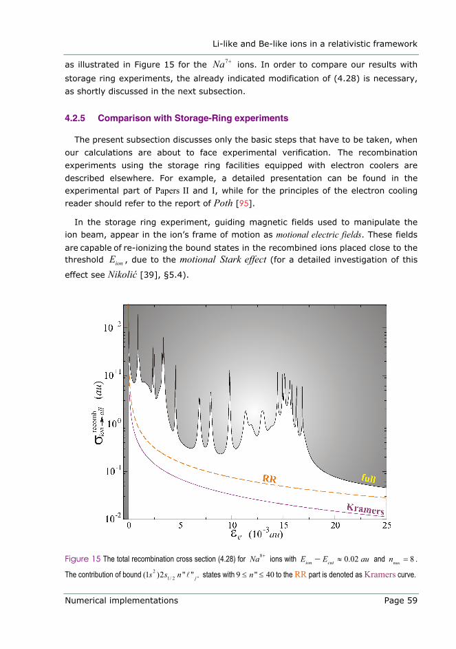
Li-like and Be-like ions in a relativistic framework
Numerical implementations Page 59
as illustrated in Figure 15 for the 7Na + ions. In order to compare our results with
storage ring experiments, the already indicated modification of (4.28) is necessary,
as shortly discussed in the next subsection.
4.2.5 Comparison with Storage-Ring experiments
The present subsection discusses only the basic steps that have to be taken, when our calculations are about to face experimental verification. The recombination
experiments using the storage ring facilities equipped with electron coolers are
described elsewhere. For example, a detailed presentation can be found in the
experimental part of Papers II and I, while for the principles of the electron cooling
reader should refer to the report of Poth [95].
In the storage ring experiment, guiding magnetic fields used to manipulate the
ion beam, appear in the ion’s frame of motion as motional electric fields. These fields
are capable of re-ionizing the bound states in the recombined ions placed close to the threshold ionE , due to the motional Stark effect (for a detailed investigation of this
effect see Nikolić [39], §5.4).
Figure 15 The total recombination cross section (4.28) for 8Na + ions with 0.02ion cutE E au≈− and max 8n = .
The contribution of bound 21/ 2 "(1 )2 " " js s n states with 9 " 40n≤ ≤ to the RR part is denoted as Kramers curve.
Li-like and Be-like ions in a relativistic framework
Page 60 Numerical implementations
In order to simulate these facts, the summation over the bound states in Eq (4.28), has to be truncated at the field cut energy cut ionE E< . Even then, due to the
limited computational resources, it is not possible to include all the bound 2
1/ 2 "(1 )2 " " js s n states below the cutE , but only up to some optimal principal
quantum number maxn . This value is chosen in a way not to affect the completion of the
DR channel; however, the RR channel will be incomplete. The missing portion of the
RR channel is usually small and estimated by Kramers formula, as illustrated in
Figure 15. As can be seen from Figure 15, the resonant dielectronic part of the full
recombination cross section (4.28) dominates over the non-resonant RR part by two
orders of magnitude.
Unfortunately, the total recombination cross section (4.28) is not directly
comparable with storage-ring experiments, and has to be converted into the
measurable recombination rate coefficient, defined as
3( ) ( ) ( )recomb
velocityspace
ion alld v f v v vα σ →∆ = − ∆∫∫∫ , (4.29)
where ( )f v is the flattened Maxwell-Boltzmann velocity distribution function
illustrated in Figure 7 of Nikolić [39], and ∆ is the relative longitudinal velocity
detuning between merged ion and electron beams. This type of velocity distribution
comes from the simultaneous acceleration and adiabatic expansion of the electron
beam in the electron cooler, with properties that are substantially different from the
regular Maxwell-Boltzmann distribution (1.3). One way of solving (4.29), is based on adaptive Gauss-Kronrod energy space integration by the means of the newly
developed RateCoeff program, details of which can be found in the attached Report
of Nikolić [39]. In this way, for a specific experimental setting, theoretical (4.29)
and experimental rate coefficients can be compared on the absolute scale, as done in Papers II and I, with an overall agreement.
Dragan Nikolié Page 61
Concluding Remarks
The purpose of work described in this thesis has been to computationally study the 0n∆ = dielectronic resonances in recombination spectra of lithium-like ions
(Papers II and I), develop and test a method to overcome the intruder state problem
as an obstacle to convergence of conventional calculations (Paper III).
In Paper I, we have also discussed the issues related to systematic comparison of
our results with storage-ring recombination experiments, in particular the role of
motional Stark effect, revealing dramatic influence on theoretical predictions. However, in Paper II they ought to be unimportant for the investigated collisional
energies. The interference between radiative and dielectronic recombination channels has been theoretically addressed in Paper I, without firm experimental
confirmation due to low signal-to-noise ratio in experimental data.
In section 3.3 we stated that our goal has been to develop a method which would
enable us to obtain a better description of autoionizing doubly excited states infected by intruder state problem. The section 4.1.3 and Paper III demonstrate that
we have indeed been able to meet this goal.


Acknowledgements
Every Ph.D. is a reflection of intellectual ripening that involves the student and supervisor's guidance and help when needed. This binary interaction takes place in the academic ambience that I have been privileged to be part of. It is always hard to adequately acknowledge vivid intellectual exchange, but let me try.
I wish to express my sincere gratitude to Professor Reinhold Schuch, for providing me with the opportunity to become a part of the Atomic Physics group.
I feel deeply indebted to my supervisor, Professor Eva Lindroth, for her knowledgeable guidance and never ceasing patience.
Much of insight and interest in Linux I owe to the advice of Dr Josef Anton, which I found indispensable during this work.
For creating a pleasant working atmosphere, I want to thank all the former and present members of Atomic Physics group.
Finally, special thanks to my wife, Violeta, who has given me a wealth of inspiration and joy, for her endless support during the time I have spent working on this thesis.
Stockholm, April 2004
Dragan Nikolić
Page 64 Dragan Nikolié
Bibliography
[ 1] I. H. Hutchinson et al, First results from Alcator-C-MOD, Phys. Plasmas 1, 1511 (1994). [ 2] C. DeMichelis and M. Mattioli, Spectroscopy and impurity behaviour in fusion plasmas,
Rep. Prog. Phys. 47, 1233 (1984). [ 3] F. Wagner and K. Lackner, in Physics of Plasmas - Wall Interactions in Controlled Fusion,
edited by D. Post and R. Behrisch (Plenum, New York, 1984). [ 4] H. S. W. Massey and D. R. Bates, The properties of neutral and ionized atomic oxygen and
their influence on the upper atmosphere, Rep. Prog. Phys. 9, 62 (1942). [ 5] M. J. Seaton and P. J. Storey, in Atomic processes and applications, edited by P. G. Burke
and B. L. Moiseiwitsch, (North Holland, 1976, p. 134). [ 6] R. H. Bell and M. J. Seaton, Dielectronic recombination: I. General theory, J. Phys. B: At.
Mol. Phys. 18, 1589 (1985). [ 7] J. Dubau and S. Volonté, Dielectronic recombination and its applications in astronomy,
Rep. Prog. Phys. 43, 199 (1980). [ 8] L. J. Roszman, in Physics of Electronic and Atomic Collisions, edited by S. Datz (North
Holland, Amsterdam, 1982, p. 641). [ 9] G. Alber, J. Cooper, and A. R. P. Rau, Unified treatment of radiative and dielectronic
recombination, Phys. Rev. A 30, 2845 (1984). [10] M. Lamoureux and N. Avdonina, Bremsstrahlung in hot plasmas with partially ionized
atoms, Phys. Rev. E 55, 912 (1997). [11] L. B. Zhao and S. C. Li, Direct radiative capture of electrons by average ions, J. Phys. B
30, 4123 (1997). [12] E. Majorana, Teoria dei tripletti P' incompleti, Nuovo Cimento 8, 107 (1931). [13] A. G. Shenstone, Ultra-Ionization Potentials in Mercury Vapor, Phys. Rev. 38, 873 (1931) [14] E. U. Condon and G. H. Shortley, The Theory of Atomic Spectra (CUP, 1935). [15] T. Rescigno and V. McKoy, Rigorous method for computing photoabsorption cross
sections from a basis-set expansion, Phys. Rev. A 12, 522 (1975). [16] D. E. Osterbrock, Astrophysics of Gaseous Nebulae and Active Galactic Nuclei
(University Science Books, Mill Valley CA, 1989). [17] H. Beutler, Über Absorptionsserien von Argon, Krypton und Xenon zu Termen zwischen
den beiden Ionisierungsgrenzen 2Po3/2 und 2Po
1/2, Z. Phys. 93, 177 (1935). [18] U. Fano, Sullo spettro di assorbimento dei gas nobili press oil limite dello spettro d’arco,
Nuovo Cimento 12, 154 (1935). [19] U. Fano, Effects of Configuration Interaction on Intensities and Phase Shifts, Phys. Rev.
124, 1866 (1961). [20] R. P. Madden and K. Codling, New Autoionizing Atomic Energy Levels in He, Ne, and
Ar, Phys. Rev. Lett. 10, 516 (1963). [21] J. W. Cooper, U. Fano and F. Prats, Classification of Two-Electron Excitation Levels of
Helium, Phys. Rev. Lett. 10, 518 (1963). [22] F. Penent et al, Observation of Triplet Doubly Excited States in Single Photon Excitation
from Ground State Helium, Phys. Rev. Lett. 86, 2758 (2001). [23] J.G. Lambourne et al, Experimental Determination of the Lifetime for the 2p3d(1Po)
Helium Doubly Excited State, Phys. Rev. Lett. 90, 153004 (2003). [24] A. Messiah, Quantum Mechanics I and II, (Amsterdam, North-Holland, 1965). [25] W. Greiner, Relativistic Quantum Mechanics, (NY Springer-Verlag, 3rd Edition, 2000).
Page 65
[26] B. Thaller, The Dirac Equation, (Springer-Verlag 1992). [27] P. A. M. Dirac, Quantised Singularities in the Electromagnetic Field, Proc. Roy. Soc. A
133, 60 (1931). [28] G. E. Brown, The Relativistic Many-Body Theory, Physica Scripta 36, 71 (1987) [29] G. Breit, The Effect of Retardation on the Interaction of two Electrons, Phys. Rev. 34, 375
(1929); Phys. Rev. 34, 553-573 (1929). [30] G. Breit, The Fine Structure of He as a Test of the Spin Interactions of Two Electrons,
Phys.Rev.36, 383(1930); Dirac's Equation and the Spin-Spin Interactions of Two Electrons, Phys.Rev.39,616 (1932).
[31] J. Sucher, Foundations of the relativistic theory of many-electron atoms, Phys. Rev. A 22, 348 (1980); Erratum: Phys. Rev. A 23, 388 (1981).
[32] I. Lindgren, Gauge dependence of interelectronic potentials, J. Phys. B 23, 1085 (1990). [33] J. B. Mann and W. R. Johnson, Breit Interaction in Multielectron Atoms, Phys. Rev. A 4,
41 (1971). [34] E. Lindroth et al, Self-consistent treatment of the Breit interaction, with application to the
electric dipole moment in thallium, J. Phys. B 22, 2447 (1989); E. Lindroth, A. Mårtensson-Pendrill, Further analysis of the complete Breit interaction, Phys. Rev. A 39, 3794 (1989).
[35] C. Froese-Fischer, Computational Atomic Structure: An MCHF Approach, (Institute of Physics Publishing, Bristol and Philadelphia, 1997, p. 152).
[36] W. E. Lamb, Jr. and R. C. Retherford, Fine Structure of the Hydrogen Atom by a Microwave Method, Phys. Rev. 72, 241 (1947).
[37] M. G. H. Gustavsson, Hyperfine Structure Calculations for Highly Charged Hydrogen-Like Ions, Ph.D. Thesis, Chalmers-Göteborg University (2000).
[38] E. A. Uehling, Polarization Effects in the Positron Theory, Phys. Rev. 48, 55 (1935). [39] D. Nikolić, Dielectronic Recombination of lithium like Ions: A Calculational Approach,
Licentiate Thesis, Stockholm University (2003). [40] I. Lindgren and J. Morrison, Atomic Many-Body Theory, 2nd ed. (S-V, Berlin, 1986). [41] T. H. Schuchan and H. A. Weidenmuller, Perturbation Theory for the Effective Interaction
in Nuclei, Annals of Physics 76, 483 (1973) [42] J. P. Finley, R. K. Chaudhuri and K. F. Freed, Applications of multireference perturbation
theory to potential energy surfaces by optimal partitioning of H: intruder states avoidance and convergence enhancement, J. Chem. Phys. 103, 4990 (1995).
[43] E. Lindroth, Calculation of doubly excited states of helium with a finite discrete spectrum, Phys. Rev. A 49, 4473 (1994).
[44] J. H. Van Vleck, On sigma-Type Doubling and Electron Spin in the Spectra of Diatomic Molecules, Phys. Rev. 33, 467 (1929).
[45] O. M. Jordahl, The Effect of Crystalline Electric Fields on the Paramagnetic Susceptibility of Cupric Salts, Phys. Rev. 45, 87 (1933).
[46] C. E. Soliverez, An effective Hamiltonian and time-independent perturbation theory, J. Phys. C 2, 2161 (1969).
[47] C. Bloch, Sur la théorie des perturbations des états liés, Nucl. Phys. 6, 329 (1958). [48] J. Cloizeaux, Extension d’une formule de Lagrange à des problèmes de valeurs propres,
Nucl. Phys. 20, 321 (1960). [49] F. Jørgensen, Effective Hamiltonians, Mol. Phys. 29, 1137 (1975). [50] I. Lindgren, The Rayleigh-Schrödinger perturbation and the linked-diagram theorem for a
multi-configurational model space, J. Phys. B 7, 2441 (1974); A Coupled-Cluster Approach to the Many-Body Perturbation Theory for Open-Shell Systems, Int. J. Quant.
Page 66
Chem.: Quant. Chem. Symp. 12, 33 (1978); Hermitian formulation of the coupled-cluster approach, J. Phys. B 24, 1143 (1991).
[51] P. Durand, Direct determination of effective Hamiltonians by wave-operator methods. I. General formalism, Phys. Rev. A 28, 3184 (1983).
[52] P. Durand and J. P. Malrieu, Effective Hamiltonians and Pseudo-Operators as Tools for Rigorous Modelling, in Ab Initio Methods in Quantum Chemistry, Part I, Ed. K. P. Lawley, John Wiley & Sons Ltd. (1987), p. 321.
[53] S. Evangelisti, J. P. Daudey and J. P. Malrieu, Qualitative intruder-state problem in effective Hamiltonian theory and their solution through intermediate Hamiltonians, Phys. Rev. A 35, 4930 (1987).
[54] J. M. Rost et al, Resonance parameters of photo doubly excited helium, J. Phys. B 30, 4663 (1997)
[55] A. Bürgers, N. Brandefelt and E. Lindroth, The interelectronic angle in doubly excites states and the quality of approximate quantum numbers, J. Phys. B 31, 3181 (1998).
[56] C. D. Lin, Classification and supermultiplet structure of doubly excited states, Phys. Rev. A 29, 1019 (1984).
[57] A. Bürgers, D. Wintgen and J. M. Rost, Highly doubly excited S states of the helium atom, J. Phys. B 28, 3163 (1995)
[58] J. P. Malrieu, P. Durand and J. P. Daudey, Intermediate Hamiltonians as a new class of effective Hamiltonians, J. Phys. A 18, 809 (1985)
[59] J. L. Heully, S. Evangelisti and P. Durand, On Some Attempts to Generalize the Effective Hamiltonian Approach, J. Phys. II France 5, 63 (1995).
[60] D. Mukhopadhyay, B. Datta (nee Kundu) and D. Mukherjee, The construction of a size-extensive intermediate Hamiltonian in a coupled-cluster framework, Chem. Phys. Lett. 197, 236 (1992).
[61] L. Meissner, Fock-space coupled-cluster method in the intermediate Hamiltonian formulation: Model with singles and doubles, J. Chem. Phys. 108, 9227 (1998).
[62] J. P. Daudey, J. L. Heully and J. P. Malrieu, Size-consistent self-consistent truncated or selected configuration interaction, J. Chem. Phys 99, 1240 (1993).
[63] A. Landau et al, Intermediate Hamiltonian Fock-space coupled-cluster method: Excitation energies of barium and radium, J. Chem. Phys. 113, 9905 (2000).
[64] A.-M. Mårtensson-Pendrill et al, Convergence of relativistic perturbation theory for the 1s2p states in low-Z helium like systems, Phys. Rev. A 51, 3630 (1995).
[65] E. Lindroth and A.-M. Mårtensson-Pendrill, (2p2) 1S state of beryllium, Phys. Rev. A 53, 3151 (1996).
[66] S. Salomonson and P. Öster, Solution of the pair equation using a finite discrete spectrum, Phys. Rev. A 40, 5559 (1989)
[67] S. Salomonson and P. Öster, Relativistic all-order pair functions from a discretized single-particle Dirac Hamiltonian, Phys. Rev. A 40, 5548 (1989)
[68] U. Fano, Correlations of two excited electrons, Rep. Prog. Phys. 46, 97 (1983). [69] S. J. Buckman and C. W. Clark, Atomic negative-ion resonances, Rev. Mod. Phys. 66,
539 (1994). [70] C. D. Lin, Hyperspherical coordinate approach to atomic and other Coulombic three-body
systems, Phys. Rep. 257, 1 (1995). [71] M. Aymar, C. H. Greene and E. Luc-Koenig, Multichannel Rydberg spectroscopy of
complex atoms, Rev. Mod. Phys. 68, 1015 (1996). [72] G. Tanner, K. Richter and J.-M. Rost, The theory of two-electron atoms: between ground
state and complete fragmentation, Rev. Mod. Phys. 72, 497 (2000).
Page 67
[73] E. Balslev and J. M. Combes, Spectral properties of many-body Schrödinger operators with dilation analytic interactions", Commun. Math. Phys. 22, 280 (1971).
[74] D. S. Tannhauser and N. Moiseyev, The solution of Lee wave problems by the complex coordinate method, Meteorologischem Zeitschrift 4, 257 (1995).
[75] K. T. Chung, T. K. Fang and Y. K. Ho, Resonances of helium in a DC field, J. Phys. B 34, 165 (2001).
[76] N. Moiseyev, Quantum theory of resonances: calculating energies, widths and cross-sections by complex scaling, Phys. Rep. 302, 211 (1998).
[77] N. Moiseyev, P. R. Certain and F. Weinhold, Resonance properties of complex-rotated Hamiltonians, Mol. Phys. 36, 1613 (1978).
[78] B. Simon, Convergence of time dependent perturbation theory for autoionizing states of atoms, Phys. Lett. A 36, 23 (1971).
[79] E.W. Weisstein, Aitken's Delta Squared Process, MathWorld - A Wolfram Web Resource, http://mathworld.wolfram.com/AitkensDeltaSquaredProcess.html
[80] D. P. Carroll, H. J. Silverstone and R. M. Metzger, Piecewise polynomial configuration interaction natural orbital study of 1s2 helium, J. Chem. Phys. 71, 4142 (1979).
[81] N. Elander, S. Levin and E. Yarevsky, Smooth exterior complex-scaling, full-angular-momentum, and three-dimensional finite-element method applied to doubly excited states of helium, Phys. Rev. A 67, 062508 (2003).
[82] I. Lindgren and D. Mukherjee, On the connectivity criteria in the open-shell coupled-cluster theory for general model spaces, Phys. Rep. 151, 93 (1987).
[83] R. F. Bishop and H. G. Kümmel, The coupled-cluster method, Phys. Today 40 (3), 52 (1987).
[84] P. Öster, Relativistic and Nonrelativistic Atomic Many-Body Calculations with Applications to Correlation Energies and to P and T Violating Electric Dipole Moments, Ph.D. Thesis, Chalmers-Göteborg University (1989).
[85] J. P. Desclaux, Relativistic Dirac-Fock Expectation Values for Atoms with Z=1 to Z=120, Atomic Data and Nuclear Data Tables 12, 311 (1973).
[86] W. R. Johnson and G. Soff, Lamb Shift in H-like Atoms, Atomic Data and Nuclear Data Tables 33, 405 (1985).
[87] S. Salomonson and P. Öster, Numerical solution of the coupled-cluster single- and double-excitation equations with application to Be and Li-, Phys. Rev. A 41, 4670 (1990)
[88] W. R. Johnson, S. A. Blundell and J. Sapirstein, Many-body perturbation-theory calculati-ons of energy levels along lithium isoelectronic sequence, Phys. Rev. A 37, 2764 (1988).
[89] P. Indelicato and P. Mohr, Coordinate-space approach to the bound-electron self-energy: Self-energy screening calculation, Phys. Rev. A 63, 052507 (2001).
[90] S. A. Blundell, Calculations of the screened self-energy and vacuum polarization in Li-like, Na-like, and Cu-like ions, Phys. Rev. A 47, 1790 (1993).
[91] S. Madzunkov et al, Dielectronic Recombination Resonances in Kr33+, Phys. Scr. T92, 357 (2001).
[92] M. Tokman et al, Dielectronic recombination resonances in F6+, Phys. Rev. A 66, 012703 (2002).
[93] M. Fogle et al, Spectroscopic study of Mg-like Ni by means of dielectronic recombination of stored ions, J. Phys. B 36, 2563 (2003).
[94] D. J. McLaughlin et al, Radiative and inner-shell dielectronic recombination in a highly charged barium ion, Phys. Rev. A 54, 2040 (1996).
[95] H. Poth, Electron cooling: Theory, experiment, application, Phys. Rep. 196, 135 (1990).

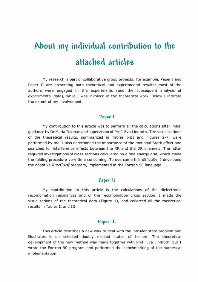
About my individual contribution to the
attached articles
My research is part of collaborative group projects. For example, Paper I and
Paper II are presenting both theoretical and experimental results; most of the
authors were engaged in the experiments (and the subsequent analysis of
experimental data), while I was involved in the theoretical work. Below I indicate
the extent of my involvement.
Paper I
My contribution to this article was to perform all the calculations after initial
guidance by Dr Maria Tokman and supervision of Prof. Eva Lindroth. The visualizations
of the theoretical results, summarized in Tables I-III and Figures 2-7, were
performed by me. I also determined the importance of the motional Stark effect and
searched for interference effects between the RR and the DR channels. The latter
required investigations of cross sections calculated on a fine energy grid, which made
the folding procedure very time consuming. To overcome this difficulty, I developed the adaptive RateCoeff program, implemented in the Fortran 90 language.
Paper II
My contribution to this article is the calculations of the dielectronic
recombination resonances and of the recombination cross section. I made the
visualizations of the theoretical data (Figure 1), and collected all the theoretical
results in Tables II and III.
Paper III
This article describes a new way to deal with the intruder state problem and
illustrates it on selected doubly excited states of helium. The theoretical
development of the new method was made together with Prof. Eva Lindroth, but I
wrote the Fortran 90 program and performed the benchmarking of the numerical
implementation.