AutoData test file for RegressIt (http://regressit.com): instructions and screen shots copied from Excel file

This is a well-known data set that is widely used to demonstrate regression software and machine learning. (See the last worksheet in the file for documentation and sources. It can be found on Kaggle and many other web sites.) There are 392 complete rows of data containing information for makes and models of cars sold in the U.S. between 1970 and 1982. The objective is to build a model for predicting fuel economy from the other variables, which include weight, horsepower, displacement, acceleration, cylinders, and country of origin. Two models have been fitted in this file, having 1 and 8 variables, and descriptive analysis has also been performed. For purposes of testing RegressIt on your computer, you just need to download the file from the Downloads web page and go to each of the analysis worksheets in it and hit either the Descriptive Statistics button or the Linear Regression button according to the sheet type, followed by Run, to verify that the various analysis options are all working. An identical output worksheet should be created, and you can hit the Last Stats or Last Model button to toggle back and forth to the original for comparison. The analyses use most of the table and graph output options at one point or another. It should only take you a few minutes to re-run all the analyses if there are no technical problems. If you do encounter technical problems, go to the tech-support web page on the RegressIt.com web site and follow the directions there. If you are not running RegressIt on your computer at the moment, just browse through the file or this document and look at the screen shots of dialog boxes as well as the output and comments in order to see what it can do. A picture of the RegressIt ribbon is shown above. As you are working, use the buttons on RegressIt's ribbon to move around in the file and to move up and down on worksheets. You'll find that this a more effficient way to navigate the large amount of output that is in the file. Here's the fast way to run all the analyses by clicking the buttons, starting from the data worksheet: Click Right to go to Stats 1 sheet > click Descriptive Statistics > click Run and wait for creation of Stats 3 > click Last Stats to return to Stats 1 Click Right to go to Stats 2 sheet > click Descriptive Statistics > click Run and wait for creation of Stats 4 > click Last Stats TWICE to go to to Stats 2 and back to Stats 4 Click Right to go to Model 1.0 sheet > click Linear Regression > click Run and wait for creation of Model 1.1 > click Last Model to return to Model 1.0 Click Right to go to Model 2.0 sheet > click Linear Regression > click Run and wait for creation of Model 2.1 > click Last Model to return to Model 2.0 Click Right to go to Model 3.0 sheet > click Linear Regression > click Run and wait for creation of Model 3.1 > click Last Model to return to Model 3.0 Click the Data button at any time to return to this sheet, click the Summaries button at any time to go to the Model Summaries sheet. Click the History button at any time for an annotated list of all sheets in the file, with details of models, from which you can jump directly to any one of them. You will note that new stats sheets and new model sheets are assigned default names in ascending order of names not already taken. For example, Stats 1 is followed by Stats 3 by default because Stats 2 is already taken. Model 1.0 if is followed by Model 1.1 by default, incrementing only the last digit. You can change the default names at run time if you wish. Also note that all stats sheets are grouped together on the left in chronological order and all model sheets are grouped together on the right. Although it will take only a couple of minutes to carry out the steps above, it is recommended that you take some more time to read these notes and study the output and additional notes on each sheet, which deal with regression in general as well as features of RegressIt. If you are new to the subject, don't be overwhelmed by

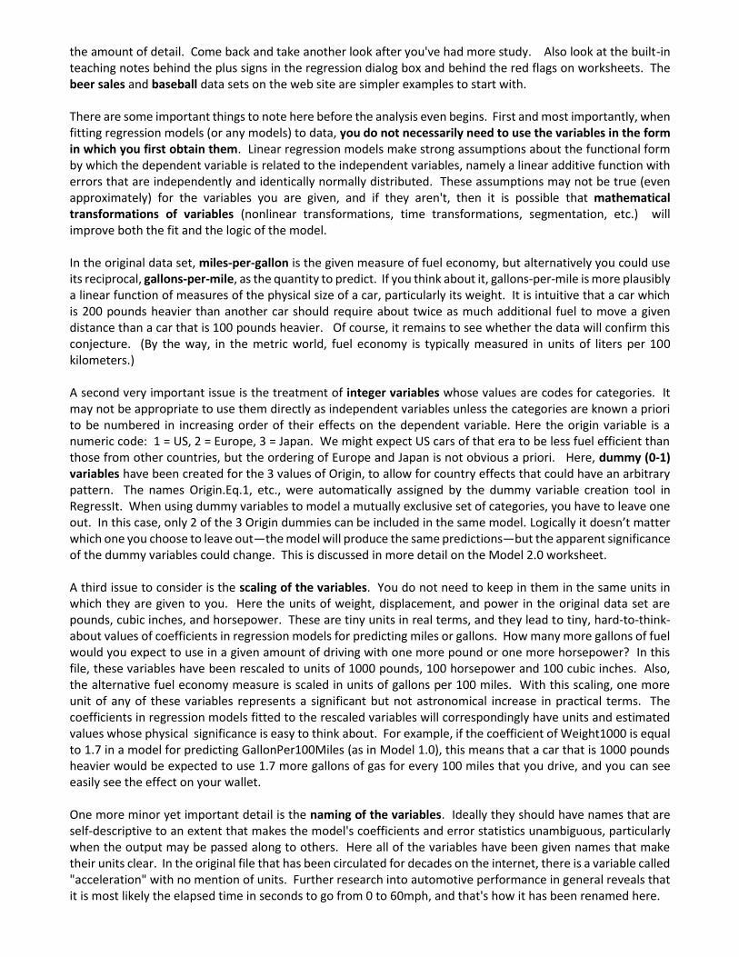
the amount of detail. Come back and take another look after you've had more study. Also look at the built-in teaching notes behind the plus signs in the regression dialog box and behind the red flags on worksheets. The beer sales and baseball data sets on the web site are simpler examples to start with.

There are some important things to note here before the analysis even begins. First and most importantly, when fitting regression models (or any models) to data, you do not necessarily need to use the variables in the form in which you first obtain them. Linear regression models make strong assumptions about the functional form by which the dependent variable is related to the independent variables, namely a linear additive function with errors that are independently and identically normally distributed. These assumptions may not be true (even approximately) for the variables you are given, and if they aren't, then it is possible that mathematical transformations of variables (nonlinear transformations, time transformations, segmentation, etc.) will improve both the fit and the logic of the model. In the original data set, miles-per-gallon is the given measure of fuel economy, but alternatively you could use its reciprocal, gallons-per-mile, as the quantity to predict. If you think about it, gallons-per-mile is more plausibly a linear function of measures of the physical size of a car, particularly its weight. It is intuitive that a car which is 200 pounds heavier than another car should require about twice as much additional fuel to move a given distance than a car that is 100 pounds heavier. Of course, it remains to see whether the data will confirm this conjecture. (By the way, in the metric world, fuel economy is typically measured in units of liters per 100 kilometers.) A second very important issue is the treatment of integer variables whose values are codes for categories. It may not be appropriate to use them directly as independent variables unless the categories are known a priori to be numbered in increasing order of their effects on the dependent variable. Here the origin variable is a numeric code: 1 = US, 2 = Europe, 3 = Japan. We might expect US cars of that era to be less fuel efficient than those from other countries, but the ordering of Europe and Japan is not obvious a priori. Here, dummy (0-1) variables have been created for the 3 values of Origin, to allow for country effects that could have an arbitrary pattern. The names Origin.Eq.1, etc., were automatically assigned by the dummy variable creation tool in RegressIt. When using dummy variables to model a mutually exclusive set of categories, you have to leave one out. In this case, only 2 of the 3 Origin dummies can be included in the same model. Logically it doesn’t matter which one you choose to leave out—the model will produce the same predictions—but the apparent significance of the dummy variables could change. This is discussed in more detail on the Model 2.0 worksheet. A third issue to consider is the scaling of the variables. You do not need to keep in them in the same units in which they are given to you. Here the units of weight, displacement, and power in the original data set are pounds, cubic inches, and horsepower. These are tiny units in real terms, and they lead to tiny, hard-to-think-about values of coefficients in regression models for predicting miles or gallons. How many more gallons of fuel would you expect to use in a given amount of driving with one more pound or one more horsepower? In this file, these variables have been rescaled to units of 1000 pounds, 100 horsepower and 100 cubic inches. Also, the alternative fuel economy measure is scaled in units of gallons per 100 miles. With this scaling, one more unit of any of these variables represents a significant but not astronomical increase in practical terms. The coefficients in regression models fitted to the rescaled variables will correspondingly have units and estimated values whose physical significance is easy to think about. For example, if the coefficient of Weight1000 is equal to 1.7 in a model for predicting GallonPer100Miles (as in Model 1.0), this means that a car that is 1000 pounds heavier would be expected to use 1.7 more gallons of gas for every 100 miles that you drive, and you can see easily see the effect on your wallet. One more minor yet important detail is the naming of the variables. Ideally they should have names that are self-descriptive to an extent that makes the model's coefficients and error statistics unambiguous, particularly when the output may be passed along to others. Here all of the variables have been given names that make their units clear. In the original file that has been circulated for decades on the internet, there is a variable called "acceleration" with no mention of units. Further research into automotive performance in general reveals that it is most likely the elapsed time in seconds to go from 0 to 60mph, and that's how it has been renamed here.

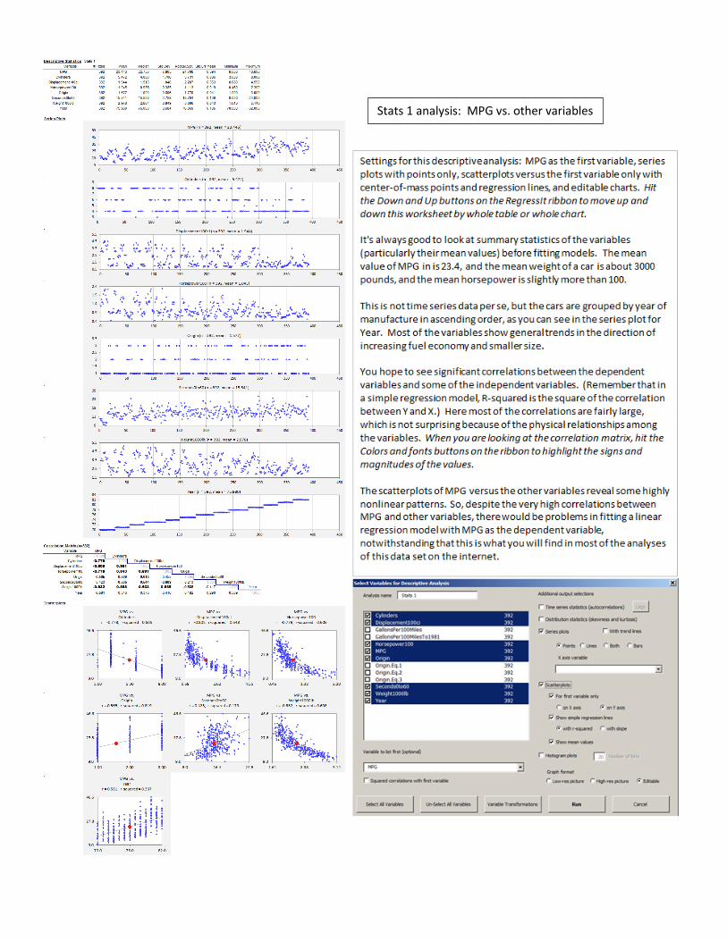
Stats 1 analysis: MPG vs. other variables

Stats 2 analysis: GallonsPer100miles vs. other variables

Model 1.0 analysis: Simple regression of GallonsPer100Miles on Weight1000lb

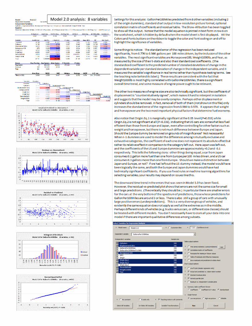
Model 2.0 analysis: 8 variables

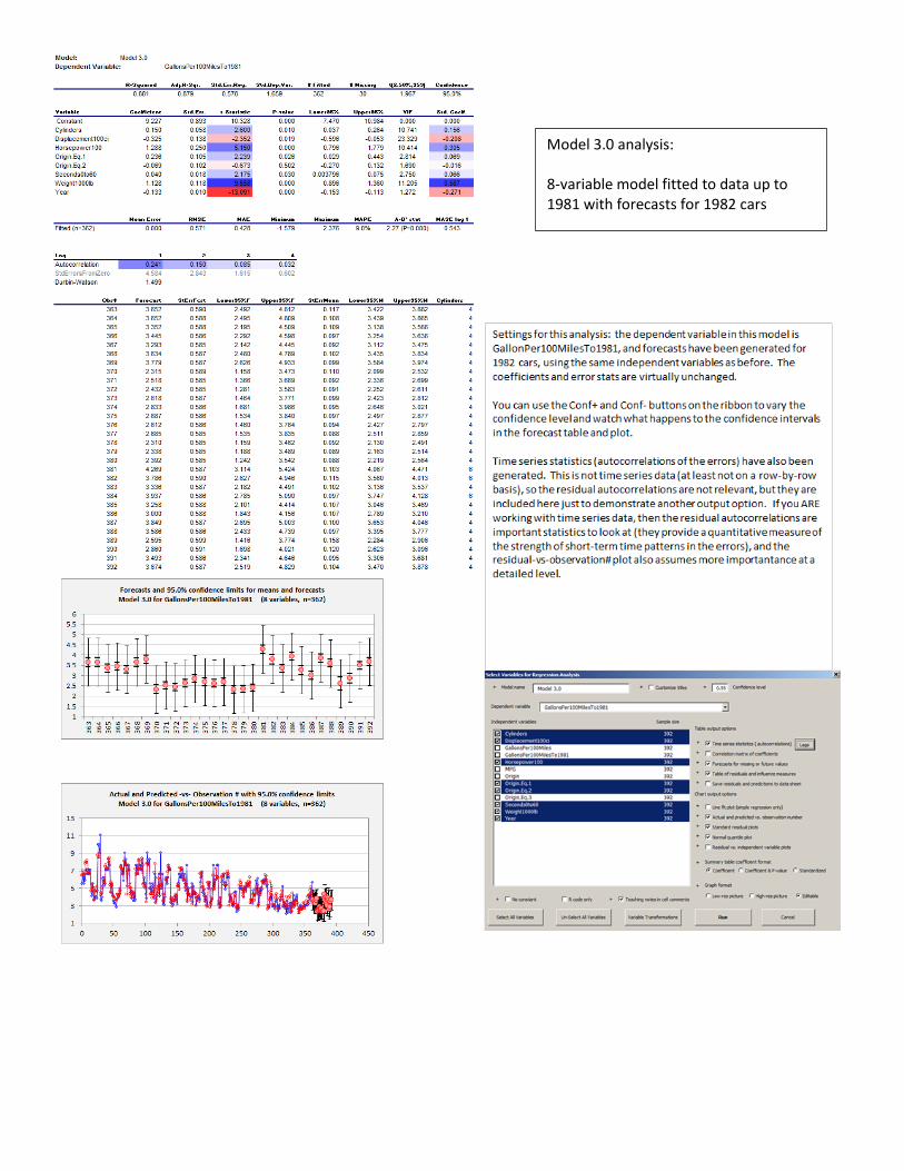
Model 3.0 analysis: 8-variable model fitted to data up to 1981 with forecasts for 1982 cars

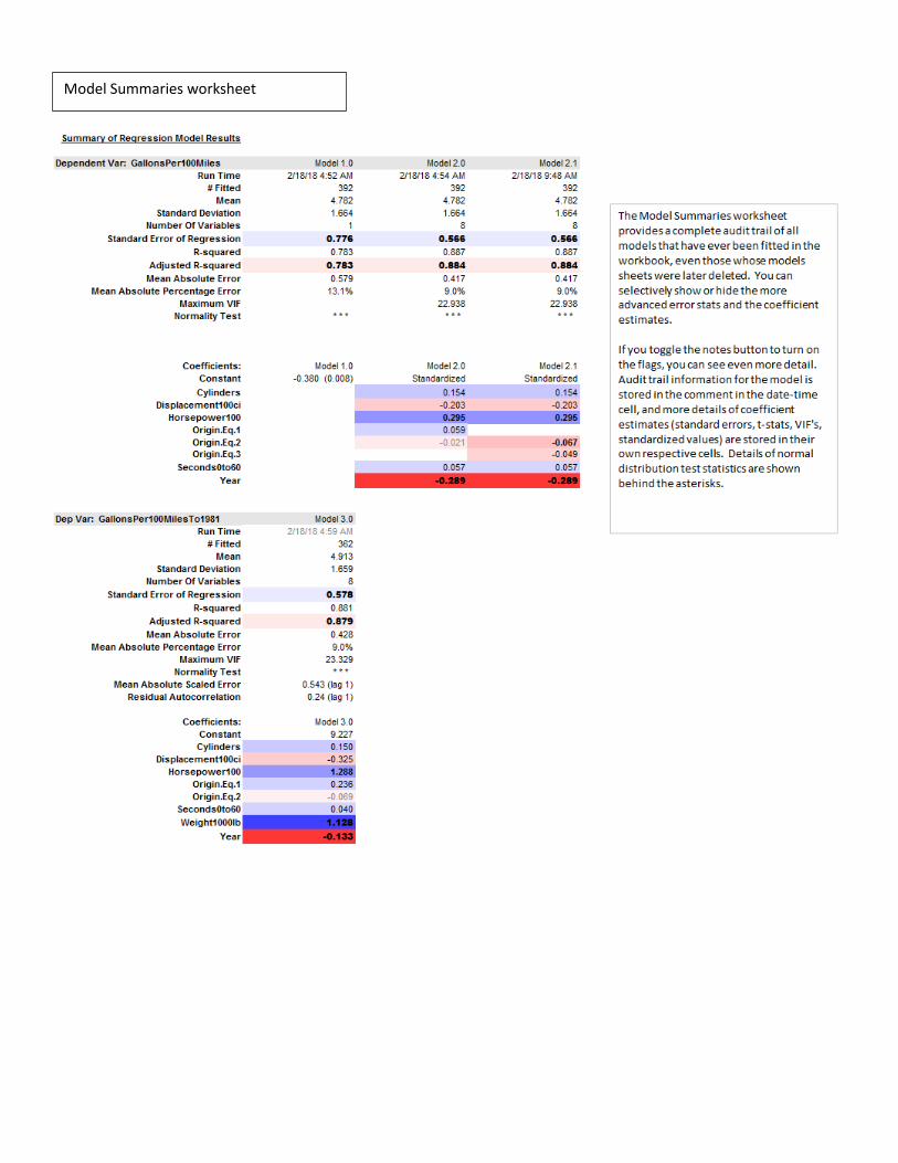
Model Summaries worksheet