ORNL/LTR-2015/780 ORNL/PTS/60609

Autocorrelation Function Statistics and Implication to Decay Ratio Estimation

José March-Leuba

Oak Ridge National Laboratory

December 2015

Approved for public release. Distribution is unlimited.

ii

DOCUMENT AVAILABILITY

Reports produced after January 1, 1996, are generally available free via the U.S. Department of Energy (DOE) Information Bridge. Web site http://www.osti.gov/bridge Reports produced before January 1, 1996, may be purchased by members of the public from the following source. National Technical Information Service 5285 Port Royal Road Springfield, VA 22161 Telephone 703-605-6000 (1-800-553-6847) TDD 703-487-4639 Fax 703-605-6900 E-mail info@ntis.gov Web site http://www.ntis.gov/support/ordernowabout.htm Reports are available to DOE employees, DOE contractors, Energy Technology Data Exchange (ETDE) representatives, and International Nuclear Information System (INIS) representatives from the following source. Office of Scientific and Technical Information P.O. Box 62 Oak Ridge, TN 37831 Telephone 865-576-8401 Fax 865-576-5728 E-mail reports@osti.gov Web site http://www.osti.gov/contact.html

This report was prepared as an account of work sponsored by an agency of the United States Government. Neither the United States Government nor any agency thereof, nor any of their employees, makes any warranty, express or implied, or assumes any legal liability or responsibility for the accuracy, completeness, or usefulness of any information, apparatus, product, or process disclosed, or represents that its use would not infringe privately owned rights. Reference herein to any specific commercial product, process, or service by trade name, trademark, manufacturer, or otherwise, does not necessarily constitute or imply its endorsement, recommendation, or favoring by the United States Government or any agency thereof. The views and opinions of authors expressed herein do not necessarily state or reflect those of the United States Government or any agency thereof.

iii

TABLE OF CONTENTS

Page Table of Contents ....................................................................................................................... iii List of Figures ............................................................................................................................ iv

List of Tables ............................................................................................................................. iv

1.0 Introduction ..................................................................................................................... 1

2.0 Model Description ............................................................................................................ 2

3.0 Sample Autocorrelation Statistics .................................................................................... 4

4.0 Decay Ratio Estimation ..................................................................................................13

5.0 Conclusions ....................................................................................................................15

iv

LIST OF FIGURES

Page Figure 1. Example of a noisy signal 1

Figure 2. Example of an unconverged noisy correlation 2

Figure 3. DR=0.2, 12 cycles 5

Figure 4. DR=0.2, 24 cycles 5

Figure 5. DR=0.2, 48 cycles 6

Figure 6. DR=0.2, 96 cycles 6

Figure 7. DR=0.5, 12 cycles 7

Figure 8. DR=0.5, 24 cycles 7

Figure 9. DR=0.5, 48 cycles 8

Figure 10. DR=0.5, 96 cycles 8

Figure 11. DR=0.8, 12 cycles 9

Figure 12. DR=0.8, 24 cycles 9

Figure 13. DR=0.8, 48 cycles 10

Figure 14. DR=0.8, 96 cycles 10

Figure 15. DR=0.95, 12 cycles 11

Figure 16. DR=0.95, 24 cycles 11

Figure 17. DR=0.95, 48 cycles 12

Figure 18. DR=0.95, 96 cycles 12

Figure 19. Illustration of non-linear regression (DR=0.2, 12 cycles) 13

LIST OF TABLES

Page Table 1. DR estimated for trial runs ..........................................................................................14

1

1.0 INTRODUCTION

This document summarizes the results of a series of computer simulations to attempt to identify the statistics of the autocorrelation function, and implications for decay ratio estimation.

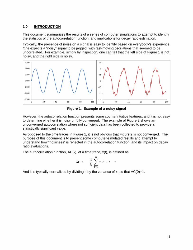
Typically, the presence of noise on a signal is easy to identify based on everybody’s experience. One expects a “noisy” signal to be jagged, with fast-moving oscillations that seemed to be uncorrelated. For example, simply by inspection, one can tell that the left side of Figure 1 is not noisy, and the right side is noisy.

Figure 1. Example of a noisy signal

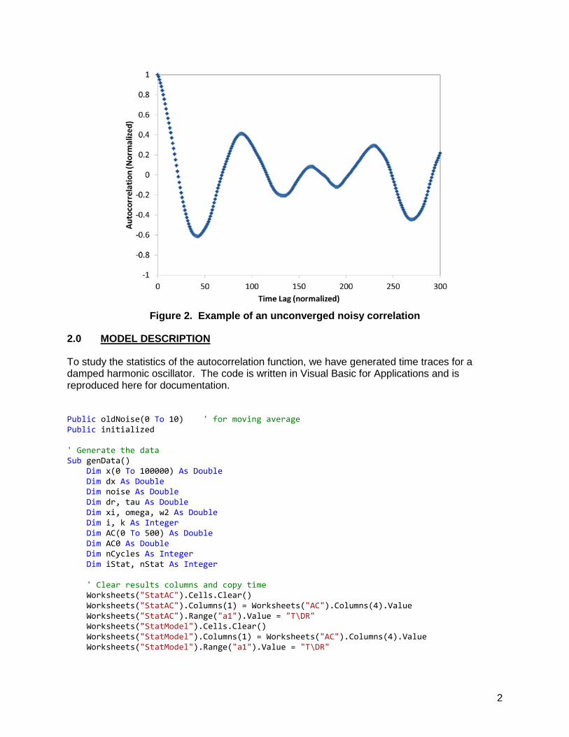
However, the autocorrelation function presents some counterintuitive features, and it is not easy to determine whether it is noisy or fully converged. The example of Figure 2 shows an unconverged autocorrelation where not sufficient data has been collected to provide a statistically significant value.

As opposed to the time traces in Figure 1, it is not obvious that Figure 2 is not converged. The purpose of this document is to present some computer-simulated results and attempt to understand how “noisiness” is reflected in the autocorrelation function, and its impact on decay ratio evaluations.

The autocorrelation function, AC(τ), of a time trace, x(t), is defined as

AC(τ) = 1𝑁

�𝑥(𝑡)𝑥(𝑡 + τ)𝑁

t=0

And it is typically normalized by dividing it by the variance of x, so that AC(0)=1.

2

Figure 2. Example of an unconverged noisy correlation

2.0 MODEL DESCRIPTION

To study the statistics of the autocorrelation function, we have generated time traces for a damped harmonic oscillator. The code is written in Visual Basic for Applications and is reproduced here for documentation.

Public oldNoise(0 To 10) ' for moving average Public initialized ' Generate the data Sub genData() Dim x(0 To 100000) As Double Dim dx As Double Dim noise As Double Dim dr, tau As Double Dim xi, omega, w2 As Double Dim i, k As Integer Dim AC(0 To 500) As Double Dim AC0 As Double Dim nCycles As Integer Dim iStat, nStat As Integer ' Clear results columns and copy time Worksheets("StatAC").Cells.Clear() Worksheets("StatAC").Columns(1) = Worksheets("AC").Columns(4).Value Worksheets("StatAC").Range("a1").Value = "T\DR" Worksheets("StatModel").Cells.Clear() Worksheets("StatModel").Columns(1) = Worksheets("AC").Columns(4).Value Worksheets("StatModel").Range("a1").Value = "T\DR"

3

' Parameters dr = Worksheets("AC").Range("b1").Value tau = Worksheets("AC").Range("b2").Value nCycles = Worksheets("AC").Range("b3").Value nStat = Worksheets("AC").Range("b4").Value ' init x(0) = 0.0# x(1) = 0.0# dx = 0.0# dx1 = 0.0# xi = Log(dr) / tau omega = 2.0# * Application.WorksheetFunction.Pi() / tau w2 = omega * omega + xi * xi ' Generate nStat correlations, fit them and save results to the Stat tab ' Note: the user must press OK (keep solver solution) for each iteration For iStat = 0 To nStat - 1 ' Generate the time data For i = 2 To 100000 x(i) = x(i - 1) + dx + lowPassGWN() dx = dx + 2 * xi * dx - w2 * x(i) Next i ' Calculate the autocorrelation and place it in the AC worksheet For k = 0 To 3 * tau AC(k) = 0.0# For i = 0 To nCycles * tau AC(k) = AC(k) + x(i) * x(i + k) Next If (k = 0) Then AC0 = AC(0) AC(k) = AC(k) / AC0 Worksheets("AC").Cells(k + 2, 4).Value = k Worksheets("AC").Cells(k + 2, 5).Value = AC(k) Next k ' Fit Correlation using Solver Call RunSolver() ' Copy AC & DR to the Stats sheet Worksheets("AC").Range("R2").Value = iStat + 1 Worksheets("StatModel").Columns(iStat + 2) = Worksheets("AC").Columns(7).Value Worksheets("StatModel").Range("B1").Offset(0, iStat).Value = Worksheets("AC").Range("O3").Value Worksheets("StatAC").Columns(iStat + 2) = Worksheets("AC").Columns(5).Value Worksheets("StatAC").Range("B1").Offset(0, iStat).Value = Worksheets("AC").Range("O3").Value Next iStat End Sub ' cheap Gaussian noise. Just add 100 uniform rand() ' mean 0, stDev~=1 Function gausNoise() As Double Dim i As Integer Dim gn As Double

4

gausNoise = 0.0# For i = 1 To 100 gausNoise = gausNoise + 2 * (Rnd() - 0.5) Next i gausNoise = gausNoise / 10 ' regain stdev=1 (haven’t test it, but should be close) End Function ' low pass gaussian - running average of the last 5 noise points Function lowPassGWN() As Double Dim i As Integer If (initilized = Null) Then oldNoise(i) = 0.0# End If For i = 0 To 9 oldNoise(i + 1) = oldNoise(i) Next oldNoise(0) = gausNoise() ' new noise lowPassGWN = 0.0# For i = 0 To 5 ' moving average lowPassGWN = lowPassGWN + oldNoise(i) Next lowPassGWN = lowPassGWN / 5.0# End Function Sub RunSolver() Worksheets("AC").Activate() SolverOk(SetCell:="$L$3", MaxMinVal:=2, ValueOf:=0, ByChange:="$L$1:$L$2", _ Engine:=1, EngineDesc:="GRG Nonlinear") SolverOk(SetCell:="$L$3", MaxMinVal:=2, ValueOf:=0, ByChange:="$L$1:$L$2", _ Engine:=1, EngineDesc:="GRG Nonlinear") SolverSolve(UserFinish:=True) End Sub

3.0 SAMPLE AUTOCORRELATION STATISTICS

A large number of sample cases have been calculated.

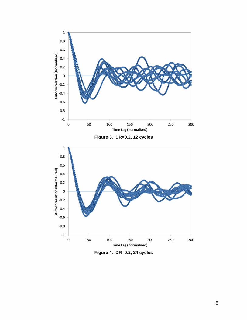
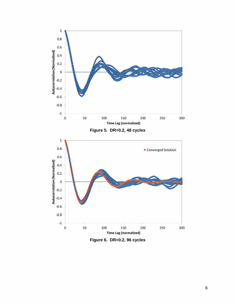
Figure 3 through Figure 6 show a composite of ten different trial calculations (using a different random noise seed) where the model corresponds to a decay ratio (DR) of 0.2 with an oscillation period of 100 units of Δt. As seen in Figure 3, the autocorrelation function is clearly unconverged when only 12 cycles (i.e., 1200 Δt’s). And even with as much as 96 cycles, the oscillations are more consistent among trials and better defined, but not fully converged.

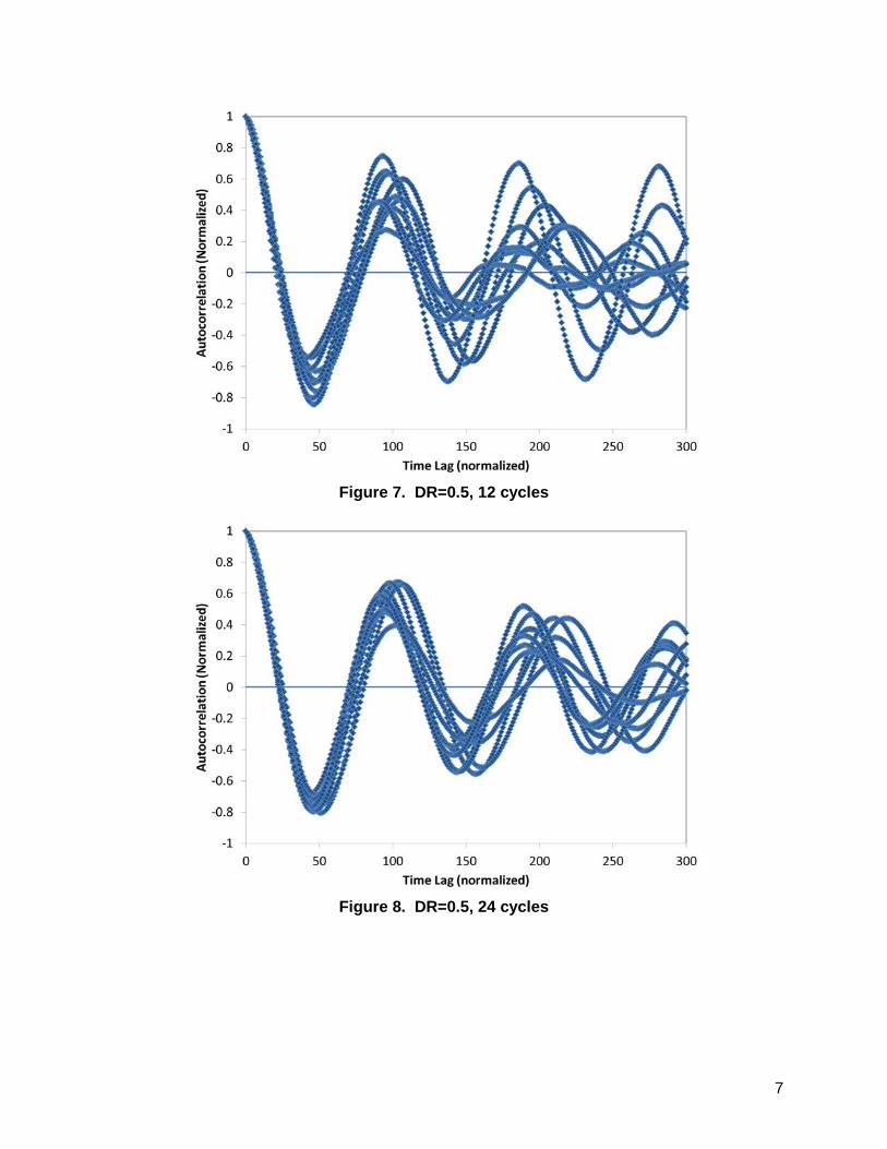
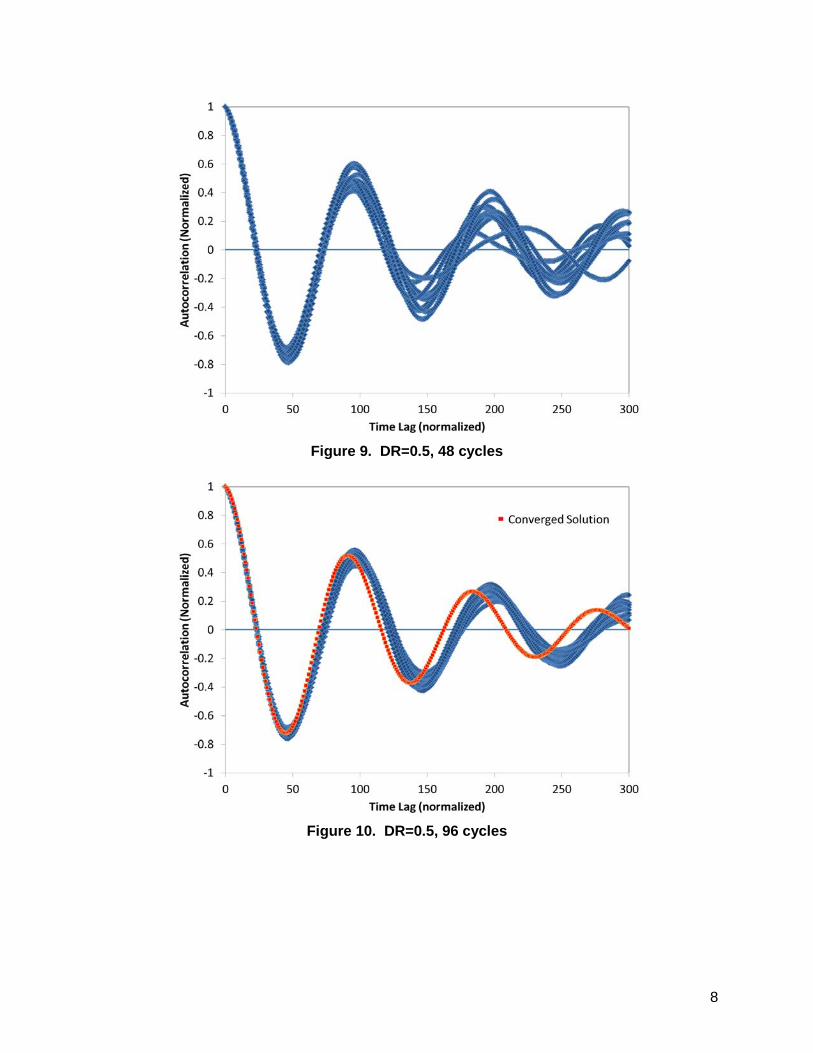
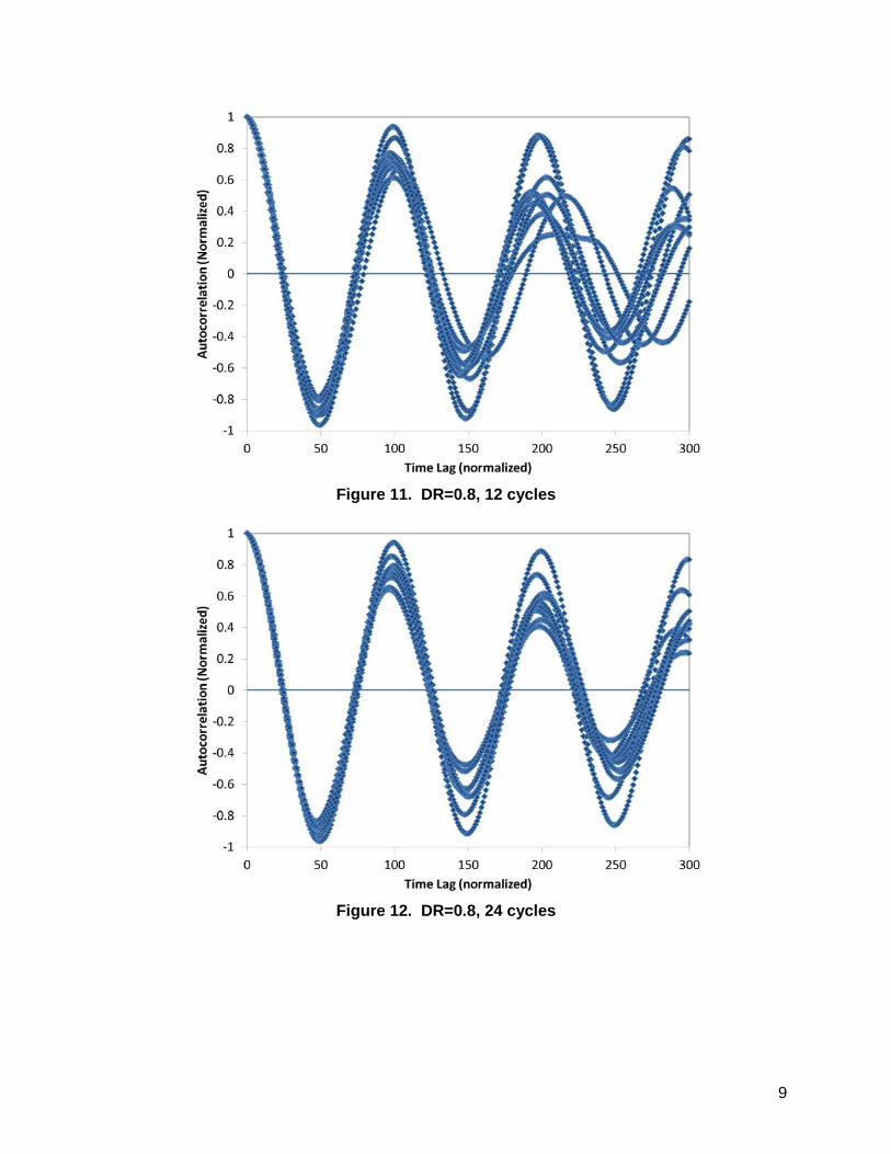
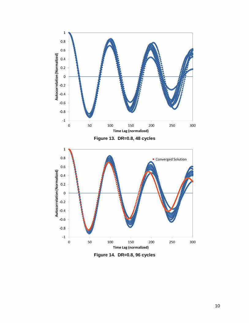
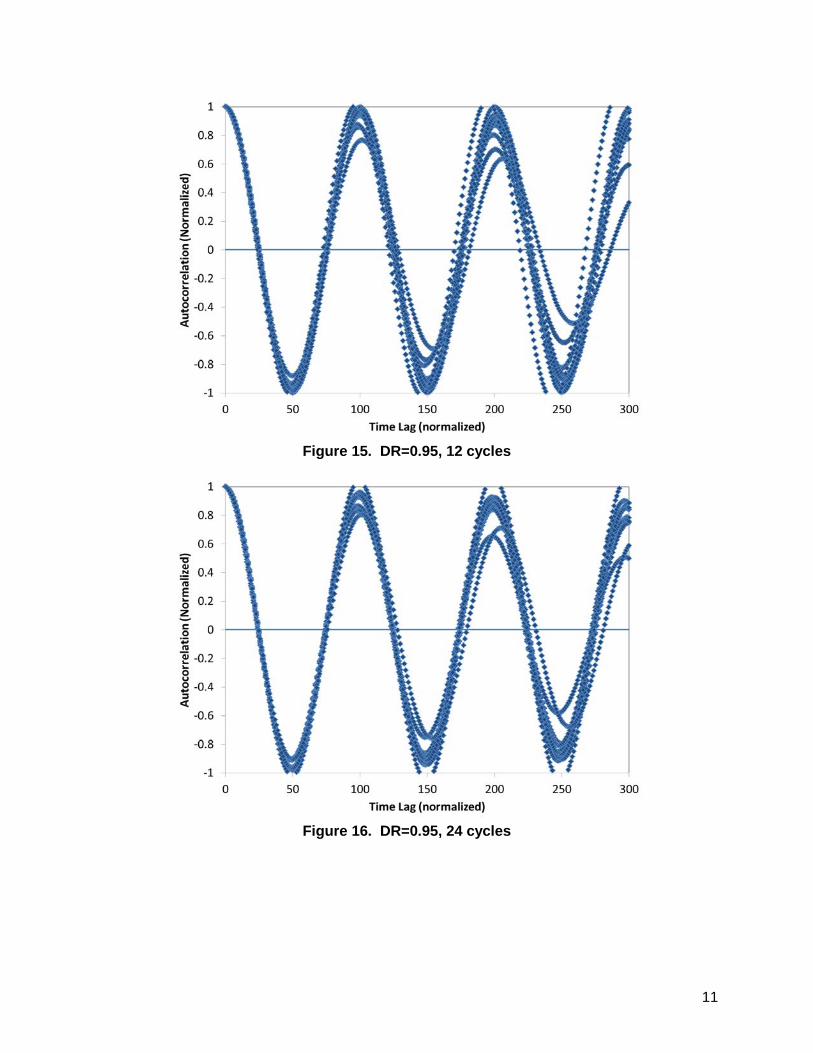
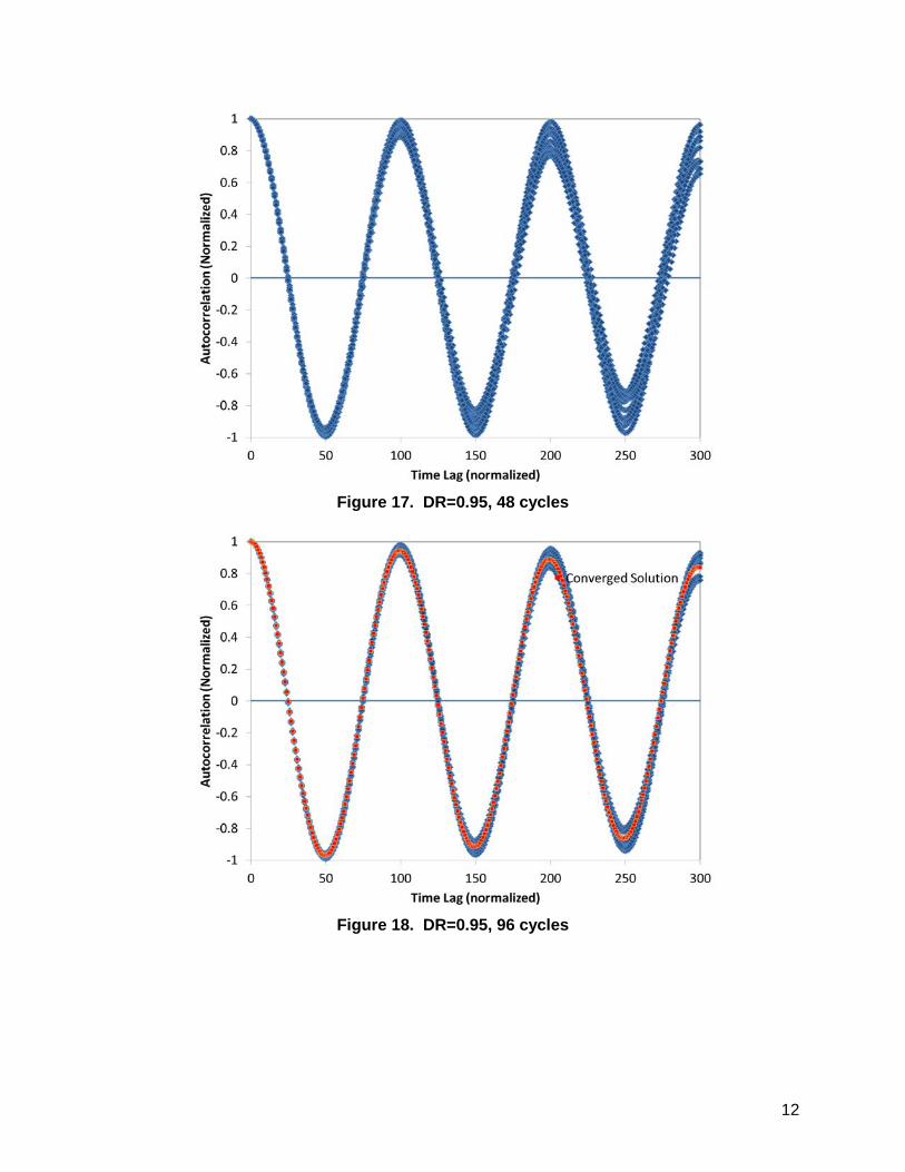
Figure 7 through Figure 10 show a similar progression with a DR of 0.5, Figure 11 through Figure 14 with a DR of 0.8, and Figure 15 through Figure 18 for a DR of 0.95. What we observe that the larger the DR (i.e., the more coherent oscillations are in the signal) the autocorrelation function converges more consistently. But, nevertheless, even with an almost unstable system (DR=0.95) and 96 cycles, attempting to identify the DR by finding the first peak in the oscillation requires very good convergence with lots and lots of data. For this reason, we propose to use a different approach to calculate the DR from the autocorrelation function.

5

Figure 3. DR=0.2, 12 cycles

Figure 4. DR=0.2, 24 cycles

6

Figure 5. DR=0.2, 48 cycles

Figure 6. DR=0.2, 96 cycles

7

Figure 7. DR=0.5, 12 cycles

Figure 8. DR=0.5, 24 cycles

8

Figure 9. DR=0.5, 48 cycles

Figure 10. DR=0.5, 96 cycles

9

Figure 11. DR=0.8, 12 cycles

Figure 12. DR=0.8, 24 cycles

10

Figure 13. DR=0.8, 48 cycles

Figure 14. DR=0.8, 96 cycles

11

Figure 15. DR=0.95, 12 cycles

Figure 16. DR=0.95, 24 cycles

12

Figure 17. DR=0.95, 48 cycles

Figure 18. DR=0.95, 96 cycles

13

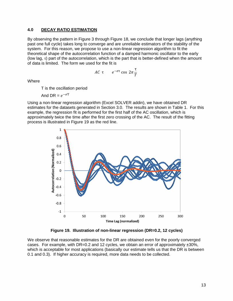
4.0 DECAY RATIO ESTIMATION

By observing the pattern in Figure 3 through Figure 18, we conclude that longer lags (anything past one full cycle) takes long to converge and are unreliable estimators of the stability of the system. For this reason, we propose to use a non-linear regression algorithm to fit the theoretical shape of the autocorrelation function of a damped harmonic oscillator to the early (low lag, τ) part of the autocorrelation, which is the part that is better-defined when the amount of data is limited. The form we used for the fit is

𝐴𝐴(τ) = 𝑒−𝜎τ cos (2𝜋τ𝑇

)

Where

T is the oscillation period

And DR = 𝑒−𝜎T

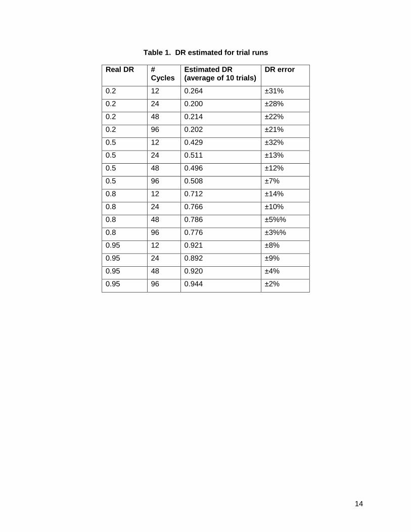
Using a non-linear regression algorithm (Excel SOLVER addin), we have obtained DR estimates for the datasets generated in Section 3.0. The results are shown in Table 1. For this example, the regression fit is performed for the first half of the AC oscillation, which is approximately twice the time after the first zero crossing of the AC. The result of the fitting process is illustrated in Figure 19 as the red line.

Figure 19. Illustration of non-linear regression (DR=0.2, 12 cycles)

We observe that reasonable estimates for the DR are obtained even for the poorly converged cases. For example, with DR=0.2 and 12 cycles, we obtain an error of approximately ±30%, which is acceptable for most applications (basically our estimate tells us that the DR is between 0.1 and 0.3). If higher accuracy is required, more data needs to be collected.

14

Table 1. DR estimated for trial runs

Real DR # Cycles

Estimated DR (average of 10 trials)

DR error

0.2 12 0.264 ±31%

0.2 24 0.200 ±28%

0.2 48 0.214 ±22%

0.2 96 0.202 ±21%

0.5 12 0.429 ±32%

0.5 24 0.511 ±13%

0.5 48 0.496 ±12%

0.5 96 0.508 ±7%

0.8 12 0.712 ±14%

0.8 24 0.766 ±10%

0.8 48 0.786 ±5%%

0.8 96 0.776 ±3%%

0.95 12 0.921 ±8%

0.95 24 0.892 ±9%

0.95 48 0.920 ±4%

0.95 96 0.944 ±2%

15

5.0 CONCLUSIONS

This paper has investigated the convergence rate and statistics of the autocorrelation function. The main conclusion from this study is that, if a limited dataset is available, the autocorrelation is likely not to be fully converged. And only the first cycle in the oscillation has any relevant information. Longer lags are randomly distributed, and unconverged. They are not a reliable indicator of the stability of the system.

We have proposed a method to estimate the decay ratio to within ±30%:

1. Identify the period of oscillation from the first zero-crossing of the autocorrelation. The period is four times the first zero-crossing.

2. Perform a linear regression to the measured AC(τ) data for time lags from 0 to approximately half the first period (the exact length of time is not crucial, and anything between 25% to 100% of the period is acceptable) using the following formula

AC(τ) = 1𝑁

�𝑥(𝑡)𝑥(𝑡 + τ)𝑁

t=0

3. The decay ratio can be estimated as DR = 𝑒−𝜎T, where T is the oscillation period

Note that care has to be exercised that the system can be represented by a simple damped harmonic oscillator. For more complex dynamic systems, this method may produce what is called the “apparent” decay ratio instead of the true “asymptotic” decay ratio, which determines the system stability. But if a ±30% accuracy is sufficient, this method is likely to produce useful results.