Author(s) Uygun, Adnan Title Monterey, California. Naval

Calhoun: The NPS Institutional ArchiveDSpace Repository

Theses and Dissertations 1. Thesis and Dissertation Collection, all items

2002-06

Network interdiction by Lagrangian relaxationand branch-and-bound

Uygun, AdnanMonterey, California. Naval Postgraduate School

http://hdl.handle.net/10945/5827

This publication is a work of the U.S. Government as defined in Title 17, UnitedStates Code, Section 101. Copyright protection is not available for this work in theUnited States.

Downloaded from NPS Archive: Calhoun

NAVAL POSTGRADUATE SCHOOL Monterey, California

THESIS

Approved for public release; distribution is unlimited.

NETWORK INTERDICTION BY LAGRANGIAN

RELAXATION AND BRANCH-AND-BOUND

by

Adnan Uygun

June 2002

Thesis Advisor: R. Kevin Wood Second Reader: Kelly J. Cormican

THIS PAGE INTENTIONALLY LEFT BLANK

i

REPORT DOCUMENTATION PAGE Form Approved OMB No. 0704-0188 Public reporting burden for this collection of information is estimated to average 1 hour per response, including the time for reviewing instruction, searching existing data sources, gathering and maintaining the data needed, and completing and reviewing the collection of information. Send comments regarding this burden estimate or any other aspect of this collection of information, including suggestions for reducing this burden, to Washington headquarters Services, Directorate for Information Operations and Reports, 1215 Jefferson Davis Highway, Suite 1204, Arlington, VA 22202-4302, and to the Office of Management and Budget, Paperwork Reduction Project (0704-0188) Washington DC 20503. 1. AGENCY USE ONLY (Leave blank)

2. REPORT DATE June 2002

3. REPORT TYPE AND DATES COVERED Master’s Thesis

4. TITLE AND SUBTITLE: Title (Mix case letters) Network Interdiction by Lagrangian Relaxatian and Branch-and-Bound 6. AUTHOR(S) Uygun, Adnan

5. FUNDING NUMBERS

7. PERFORMING ORGANIZATION NAME(S) AND ADDRESS(ES) Naval Postgraduate School Monterey, CA 93943-5000

8. PERFORMING ORGANIZATION REPORT NUMBER

9. SPONSORING / MONITORING AGENCY NAME(S) AND ADDRESS(ES) N/A

10. SPONSORING / MONITORING AGENCY REPORT NUMBER

11. SUPPLEMENTARY NOTES The views expressed in this thesis are those of the author and do not reflect the official policy or position of the Department of Defense or the U.S. Government. 12a. DISTRIBUTION / AVAILABILITY STATEMENT Approved for public release; distribution is unlimited.

12b. DISTRIBUTION CODE

13. ABSTRACT (maximum 200 words)

The maximum-flow network-interdiction problem (MXFI) arises when an interdictor, using limited interdiction

resources, wishes to restrict an adversary’s use of a capacitated network.

MXFI is not easy to solve when converted to a binary integer program. Derbes (1997) uses Lagrangian relaxation to

solve the problem, at least approximately, for a single value of available resource, R. Bingol (2001) extends this technique to

solve MXFI approximately for all integer values of R in a specified range. But, “problematic R-values” with substantial

optimality gaps do arise. We reduce optimality gaps in two ways. First, we find the best Lagrangian multiplier for problematic

R-values by following the slope of the Lagrangian function. Secondly, we apply a limited-enumeration branch-and-bound

algorithm.

We test our algorithms on six different test networks with up to 402 nodes and 1826 arcs. The algorithms are coded

in Java 1.3 and run on a 533 MHz Pentium III computer. The first technique takes at most 39.3 seconds for any problem, and

for one instance, it solves 8 of the problem’s 15 problematic R-values. For that problem, the second technique solves four of

the remaining problematic R-values, but run time increases by two orders of magnitude.

15. NUMBER OF PAGES

65

14. SUBJECT TERMS Network Interdiction, Mathematical Modeling, Lagrangian Relaxation, Branch-and-Bound

16. PRICE CODE

17. SECURITY CLASSIFICATION OF REPORT

Unclassified

18. SECURITY CLASSIFICATION OF THIS PAGE

Unclassified

19. SECURITY CLASSIFICATION OF ABSTRACT

Unclassified

20. LIMITATION OF ABSTRACT

UL

ii


iii

Approved for public release; distribution is unlimited.

NETWORK INTERDICTION BY LAGRANGIAN RELAXATION AND BRANCH-AND-BOUND

Adnan Uygun

First Lieutenant, Turkish Army B.S., Turkish Army Academy, 1997

Submitted in partial fulfillment of the requirements for the degree of

MASTER OF SCIENCE IN OPERATIONS RESEARCH

from the

NAVAL POSTGRADUATE SCHOOL June 2002

Author: Adnan Uygun

Approved by: R. Kevin Wood

Thesis Advisor

Kelly J. Cormican Second Reader

James N. Eagle Chairman, Department of Operations Research

iv


v

ABSTRACT

The maximum-flow network-interdiction problem (MXFI) arises when an

interdictor, using limited interdiction resources, wishes to restrict an adversary’s use of a

capacitated network.

MXFI is not easy to solve when converted to a binary integer program. Derbes

(1997) uses Lagrangian relaxation to solve the problem, at least approximately, for a single

value of available resource, R. Bingol (2001) extends this technique to solve MXFI

approximately for all integer values of R in a specified range. But, “problematic R-values”

with substantial optimality gaps do arise. We reduce optimality gaps in two ways. First,

we find the best Lagrangian multiplier for problematic R-values by following the slope of

the Lagrangian function. Secondly, we apply a limited-enumeration branch-and-bound

algorithm.

We test our algorithms on six different test networks with up to 402 nodes and 1826

arcs. The algorithms are coded in Java 1.3 and run on a 533 MHz Pentium III computer.

The first technique takes at most 39.3 seconds for any problem, and for one instance, it

solves 8 of the problem’s 15 problematic R-values. For that problem, the second technique

solves four of the remaining problematic R-values, but run time increases by two orders of

magnitude.

vi


vii

TABLE OF CONTENTS

I. INTRODUCTION .......................................................................................................1 A. BACKGROUND ..............................................................................................2 B. OUTLINE OF THESIS...................................................................................4

II. FUNDAMENTALS OF NETWORK INTERDICTION..........................................5 A. DEFINITIONS AND NOTATION.................................................................5 B. NETWORK INTERDICTION MODEL.......................................................6

1. Maximum Flow Network Interdiction Problem (MXFI).................6 2. An Integer Program for MXFI (MXFI-IP) .......................................7 3. Lagrangian Relaxation for MXFI (MXFI-LR) .................................8

III. NETWORK INTERDICTION BY LAGRANGIAN RELAXATION AND BRANCH-AND-BOUND ..........................................................................................11 A. PRELIMINARIES.........................................................................................11 B. THE LAGRANGIAN-RELAXATION MODEL........................................12 C. FINDING AN OPTIMAL λ FOR PROBLEMATIC R ............................18 D. RESTRICTED BRANCH-AND-BOUND ...................................................25

IV. COMPUTATIONAL RESULTS..............................................................................33 A. TEST NETWORK DESIGN ........................................................................33 B. RESULTS .......................................................................................................34

V. CONCLUSIONS AND FURTHER RESEARCH...................................................41 A. SUMMARY ....................................................................................................41 B. FURTHER RESEARCH...............................................................................42

LIST OF REFERENCES......................................................................................................45

INITIAL DISTRIBUTION LIST.........................................................................................47

viii


ix

LIST OF FIGURES Figure 1. NETSample. ...................................................................................................19 Figure 2. Lagrangian Function for ( ,1)z λ for NETSample. ...........................................19 Figure 3. Lagrangian Function of R = 2 for NETSample. ............................................21 Figure 4. Sample Enumeration Tree. ............................................................................27 Figure 5. Modified Enumeration Tree. ...........................................................................28 Figure 6. NET 3 3× . ......................................................................................................33

x


xi

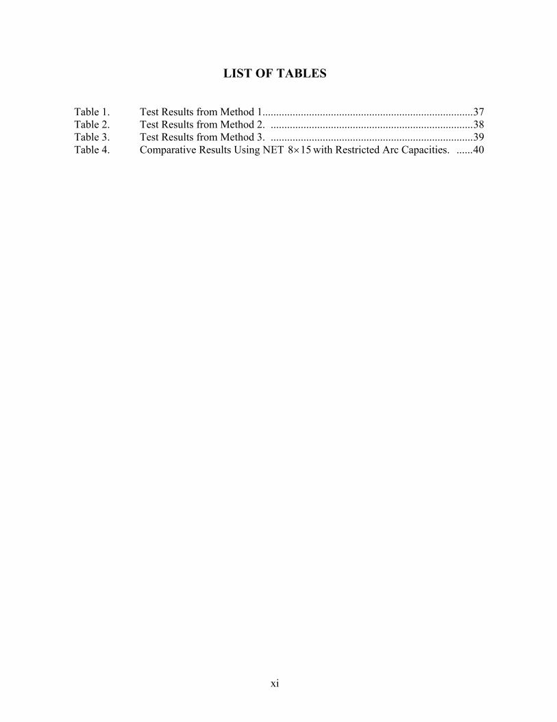
LIST OF TABLES Table 1. Test Results from Method 1.............................................................................37 Table 2. Test Results from Method 2. ..........................................................................38 Table 3. Test Results from Method 3. ..........................................................................39 Table 4. Comparative Results Using NET 8 15× with Restricted Arc Capacities. ......40

xii


xiii

ACKNOWLEDGMENTS

I must express my deepest gratitude and appreciation to Professor Kevin Wood for

his guidance, encouragement, and patience during this most challenging part of my

education at the Naval Postgraduate School. I wish to thank LCDR Kelly Cormican for his

valuable suggestions and motivational leadership. I am grateful to the Turkish Army for

providing me with the privilege of studying at NPS.

My special thanks go to my parents, Resul and Saziye Uygun, for their unending

support from thousands of miles away. Last but not least, I would like to thank my

nephew, Dorukhan Uygun, for being an inadvertent source of inspiration through his own

success.

xiv


xv

EXECUTIVE SUMMARY

This thesis is concerned with solving or approximately solving a maximum-flow

network-interdiction problem (MXFI). This problem arises when an interdictor, using

limited interdiction resources, wishes to restrict an adversary’s use of a capacitated

network. In particular, the adversary, or “network user” seeks to maximize flow through

the network, and the interdictor seeks to minimize that maximum flow by destroying arcs.

MXFI is not easy to solve when converted to a binary integer program. Derbes

(1997) uses Lagrangian relaxation to attempt to solve this problem for a single value of

interdiction resource, R. Bingol (2001) extends this technique to solve MXFI for all integer

values of R in some specified range assuming that exactly one unit of resource is required

to interdict an arc. However, about 25% of these values are “problematic” in tests, i.e.,

positive optimality gaps arise.

In our study, we first focus on decreasing the optimality gaps by finding the best

Lagrangian multiplier. We simply follow the slope of the Lagrangian function to

accomplish this. For most test problems, this method decreases the gap for problematic R-

values by approximately 50%. This method helps find better feasible solutions and

sometimes prove optimality. But, some large optimality gaps may remain.

We tackle the remaining problematic R-values with a restricted branch-and-bound

technique, which has only one level of enumeration below the root. This technique creates

a strict partition of the feasible region and the minimum lower bound from among these

partitions is a lower bound on the optimal solution value. In our tests, we solve

approximately 70% of the problematic R-values that remain after applying the first

technique. However, branch-and-bound increases run times dramatically.

Both procedures are written and compiled using the Java 1.3 programming

language. All tests are performed on a personal computer with a 533 MHz Pentium III

processor and 192 MB of RAM, running under the Windows XP operating system. For test

purposes, we have used 6 different grid networks. The smallest one has 27 nodes and 86

arcs and the largest one has 402 nodes and 1826 arcs.

xvi

Applying both techniques together, we have been able to either solve problematic

R-values exactly or improve their optimality gaps for most cases. In fact, 85% of the

problematic R-values are solved optimally in our tests. One problem with a large

optimality gap does not improve, however.

1

I. INTRODUCTION

This thesis develops a method based on Lagrangian relaxation to solve a maximum-

flow network-interdiction problem. This problem arises when an interdictor, using limited

interdiction resources, wishes to restrict an adversary’s use of a capacitated network. In

particular, the adversary, or “network user” seeks to maximize flow through the network,

and the interdictor seeks to minimize that maximum flow by destroying arcs.

The maximum-flow network-interdiction problem (MXFI), converted to an integer

program, is difficult to solve because of an interdiction-resource constraint. Derbes (1997)

uses Lagrangian relaxation to move this constraint into the objective function, and is able

to solve MXFI efficiently for certain resource levels R. However, he solves for only one

value of R at a time. The goal of this thesis is to solve MXFI efficiently for all reasonable

values of R in a single procedure.

The underlying reasons that motivate us to obtain solutions for all values of R are:

First, R may not be specified. For instance, at an early stage of planning, we may not know

how much resource will be available when the interdiction plan is to be carried out. Thus,

we would like to provide the decision-maker with solutions for all potential values of R.

Secondly, decision-makers often like to have some input on the amount of resource to be

expended. This helps them review and maybe revise their decisions. Finally, it is not

much harder to solve MXFI for all reasonable values of R than for a single value.

Derbes models the interdiction of arc k as requiring a small, integer amount of

resource, kr > 0. For the sake of simplicity, we assume kr = 1 for all interdictable arcs k,

although arcs may also be specified as non-interdictable. Derbes also considers a dynamic

version of MXFI in which flows require time to move through the network and interdicted

arcs can be repaired over time. The dynamic version of MXFI is beyond the scope of this

thesis.

Bingol (2001) investigates our version of MXFI and also attempts to solve for all R

using a Lagrangian-relaxation procedure. Essentially, he estimates the values of the

Lagrangian functions for all R simultaneously. He assumes that these functions only break

at points at which the Lagrangian multiplier equals the capacity of some arc. In carrying

2

out computations, he encounters some values of R for which his procedure cannot find an

exact solution, so he develops a heuristic to handle these cases and determines associated

optimality gaps. He does not, however, optimize the Lagrangian-based lower bounds.

In this thesis, we use a procedure similar to Bingol’s to find solutions for all values

of R but will optimize the Lagrangian lower bounds as needed. When significant

optimality gaps are identified, we apply a restricted branch-and-bound procedure to

improve the lower bounds and possibly identify better solutions. This procedure is

restricted to create enumeration trees having limited depth.

A. BACKGROUND

There are different types of network-interdiction problems. For instance, Israeli

(1999) focuses on Maximizing the Shortest Path (MXSP) to slow a network user’s

movement between two specified nodes in a network. The k-most-vital-arcs problem is a

special case of MXSP in which the interdictor seeks to destroy exactly k arcs to maximize

the shortest path length. Steinrauf (1991) designs a model to isolate a targeted demand

node in a network. Morton (2001) describes a stochastic network-interdiction model to

help detect the smuggling of stolen nuclear materials. However, in this thesis, we are only

concerned with the deterministic maximum-flow network-interdiction problem, MXFI.

The scientific literature on network interdiction begins with Wollmer (1966) who

focuses on “Removing Arcs from a Network,” where the objective is to maximize the

reduction of the flow between an origin and a destination node. Later, Wollmer (1970)

presents two algorithms for targeting strikes in an LOC (lines-of-communication) network

attempting to make the network user’s costs as large as possible over time. The LOC

networks are described by a directed network, with arcs representing road, rail, or

waterway segments. The costs in his study include both flow costs in dollars, vehicle

hours, manpower units, or any other appropriate measures; plus repair costs incurred by

strikes, measured in similar units.

McMasters and Mustin (1970) devise an algorithm to determine the optimum

interdiction plan for minimizing network flow capacity when the minimum capacity on an

arc is positive and the cost of interdiction is linear in the amount of arc capacity reduction.

3

Ratiff, Sicilia and Lubore (1975) show how to find a set of arcs, called “the N most

vital links,” whose simultaneous removal from a single-commodity flow network results in

the greatest decrease in the throughput capacity of the remaining system.

Steinrauf (1991) develops two mathematical programs to determine strategies to

interdict a network using limited resources. The first model identifies a set of arcs whose

interdiction minimizes the maximum flow through the network, constrained by the

available resources. This is essentially MXFI. The second model identifies a set of arcs to

interdict that isolates a target node and the largest possible set of contiguous nodes. The

latter model can be used if the exact location of a target node is uncertain.

Wood (1993) shows that the MXFI is NP-complete even if the interdiction of an arc

requires exactly one unit of resource. New, flexible integer-programming models are

developed for the problem and a number of variants (partial arc interdiction, multiple

sources and sinks, undirected networks, multiple resources, multiple commodities). Valid

inequalities and a reformulation are derived to tighten the LP relaxations of some of these

models.

Cormican (1995) solves MXFI using Bender’s decomposition, which takes

advantage of easy-to-solve network-flow subproblems. Cormican et al. (1998) solve

stochastic versions of MXFI where arc capacities and/or interdiction success may be

uncertain. Stochastic versions of MXFI are beyond the scope of this thesis, however.

Whiteman (1999) discusses techniques for planning the interdiction of a complex

infrastructure network to improve single-strike effectiveness. The motivation for his work

arises from the huge cost of modern weapons and delivery platforms and intolerance for

casualties, and the consequential desire to minimize the number of subsequent attacks. To

optimize target selection, he modifies the integer program developed by Wood (1993),

specifying different flow goals.

Bingol (2001) extends the earlier work by Derbes (1997) on a Lagrangian-

relaxation technique to solve MXFI for all integer values of total interdiction resource, R,

in some specified range. His basic procedure solves MXFI exactly for most values of R,

but “problematic values” of R arise with positive optimality gaps.

4

B. OUTLINE OF THESIS

This chapter has provided background on network interdiction problems and has

surveyed previous studies in this field. The following chapter explains MXFI in detail, and

develops the Lagrangian-relaxation technique for solving it, at least approximately. In

Chapter III, we first study the algorithms used by Derbes (1997) and Bingol (2001).

Subsequently, we present two new procedures to improve optimality gaps for problematic

R-values and sometimes even solve these problems exactly. Chapter IV provides the

computational results for the new procedures. Finally, Chapter V provides conclusions and

points out directions for further research.

5

II. FUNDAMENTALS OF NETWORK INTERDICTION

This chapter first defines necessary concepts and notation for our study. The

notation is similar to that used by Wood (1993) and Bingol (2001). The second part of the

chapter starts with MXFI, which is a min-max model, and develops a minimizing integer-

programming formulation (MXFI-IP) and a Lagrangian relaxation (MXFI-LR) of that

integer program.

A. DEFINITIONS AND NOTATION

G = (N, A) denotes a directed network with node set N and arc set A. An arc k = (i,

j) starts from “tail node” i and ends at “head node” j. Each arc k has a capacity uk > 0. The

network has a source node s and a sink node t. For mathematical purposes, we add to A the

artificial arc ( , )a t s= with au = ∞ . The forward star of node i, FS(i), includes all arcs of

the form (i, j). The reverse star of node i, RS(i), represents all arcs of the form (j, i).

In this study, only arc interdiction is allowed. In the test networks, rk is the amount

of interdiction resource necessary to destroy arc k. For simplicity, we assume rk = 1 or rk

= ∞; the latter case simply means the arc cannot be interdicted.

A cut (Ns, Nt) partitions the node set N into two subsets, Ns and Nt where s ∈ Ns and

t ∈ Nt. An arc (i, j) is a forward arc of cut (Ns, Nt) if i ∈ Ns and j ∈ Nt.

AC represents the set of forward arcs for cut (Ns, Nt). The capacity of a cut, u(Ns,

Nt), is the sum of the capacities of the forward arcs in that cut:

u(Ns, Nt)= ∑∈ CAk

ku .

If u(Ns, Nt) is the minimum of all cut capacities, then ( , )s tN N is a minimum cut.

We know by the maximum-flow minimum-cut theorem that the capacity of the minimum

cut equals the maximum s-t flow in that network; the maximum flow model will be

described shortly.

6

B. NETWORK INTERDICTION MODEL

Here, we define the basic MXFI, which is then converted into MXFI-IP.

Lagrangian relaxation for MXFI-IP is presented subsequently.

1. Maximum Flow Network Interdiction Problem (MXFI) In MXFI, an interdictor, using limited interdiction resources, destroys arcs of the

enemy’s network G= (N, A) and makes them useless. The objective is to minimize the

maximum amount of flow that the enemy, i.e., the network user, can transport through the

network. We define MXFI as a function of total interdiction resource R:

MXFI(R):

Indices:

i, j ∈ N nodes of network G=(N,A)

s ∈ N source node

t ∈ N sink node

k = (i, j) ∈A network arcs

a = (t, s) ∈A artificial return arc included in A

Data:

uk nominal, uninterdicted capacity of arc k

rk amount of resource necessary to interdict arc k (ra = ∞)

R total amount of available resource

Decision Variables:

yk amount of flow on arc k (network user)

xk 1 if interdiction of arc k is attempted (interdictor)

0 otherwise

7

Formulation:

( ) min max aXz R y

∈=

x y

s.t. 0)()(

=− ∑∑∈∈ iRSk

kiFSk

k yy ∀i ∈ N (1)

)1(0 kkk xuy −≤≤ ∀k ∈ A (2)

{ }where 0,1 , 0Ak k a

k AX r x R x

∈

= ∈ ≤ ≡

∑x . (3)

In this model, constraints (2) force capacities down to zero for all interdicted arcs.

For fixed x, the inner maximizing problem is a standard maximum-flow model, which

maximizes the flow from a source node to a sink node subject to flow-balance constraints

(1) and arc capacities (2). MXFI(R) can also be reformulated as MXFIR(R) (Cormican et

al. 1998):

MXFIR(R):

( ) min max a k kX k Az R y x y

∈∈

= −∑x y

s.t. 0)()(

=− ∑∑∈∈ iRSk

kiFSk

k yy ∀i ∈ N

kk uy ≤≤0 ∀k ∈ A

{ }where 0,1 , 0Ak k a

k AX r x R x

∈

= ∈ ≤ ≡

∑x .

2. An Integer Program for MXFI (MXFI-IP) Taking the dual of the inner maximization of MXFIR gives us a linear minimization

model (which is derived by Wood 1993 directly from MXFI):

8

MXFI-IP(R)

Indices: As in MXFI

Data: As in MXFI

Decision Variables:

αi 1 if i ∈ Nt and 0 if i ∈ Ns, for a model-identified cut (Ns,Nt)

βk if k is a forward arc of cut (Ns,Nt) and not interdicted, 0 otherwise

xk 1 if interdiction of arc k is interdicted, 0 otherwise (interdictor)

Formulation:

, ,

( ) min k kk A

z R u β∈

= ∑α β x

s.t. 0≥++− kkji x βαα ∀k = (i,j) ∈ A –{a} (4)

1≥++− aast x βαα for a = (t, s) (5)

Rxr kAk

k ≤∑∈

(6)

αi ∈ {0,1} ∀i ∈ N

xk , βk ∈ {0,1} ∀k ∈ A

αs ≡ 0, αt ≡ 1

βa ≡ xa ≡ 0

3. Lagrangian Relaxation for MXFI (MXFI-LR)

Lagrangian relaxation is a general solution strategy for solving mathematical

programs that permits us to decompose problems to exploit their structure. This solution

approach leads to bounds on the optimal objective function value and, frequently, to good,

though not necessarily optimal solutions (Ahuja, Magnanti and Orlin 1993, p. 601).

9

MXFI-IP can be difficult to solve because of constraint (6), so we transfer this

constraint into the objection function following Derbes (1997). After this modification, the

new model, MXFI-LR, can be easily solved, although it may not always yield an optimal

solution. The model is:

MXFI-LR (λ , R):

, ,

( , ) min ( )α β x k k k k

k A k Az R u r x Rλ β λ

∈ ∈

= + −∑ ∑ (7)

s.t. 0≥++− kkji x βαα ∀k = (i,j) ∈ A – {a}

1≥++− aast x βαα for a = (t, s)

αi ∈ {0,1} ∀i ∈ N

xk , βk ∈ {0,1} ∀k ∈ A

αs ≡ 0, αt ≡ 1

βa ≡ xa ≡ 0

The term )( Rxr kAk

k −∑∈

λ represents a penalty for exceeding or a reward for not consuming

the resource budget R. The parameter λ can be interpreted as the dual cost of interdicting

an arc.

The linear-programming relaxation of MXFIR has integer extreme points, so we

can take the dual of that relaxation to obtain MXFI-LRD after some simplifications

(Derbes 1997):

MXFI-LRD (λ , R):

RyRz a λλ −=y

max),(

s.t. 0)()(

=− ∑∑∈∈ iRSk

kiFSk

k yy ∀i ∈ N

10

},min{0 kkk ruy λ≤≤ ∀k ∈ A

Of course, z(λ,R) is only a lower bound on z(R), but we can use this lower bound,

and interdiction plans obtained during its solution to solve MXFI(R), at least

approximately. Procedures to do this are presented in the next chapter.

11

III. NETWORK INTERDICTION BY LAGRANGIAN RELAXATION AND BRANCH-AND-BOUND

This chapter explains our algorithm for solving MXFI. The algorithm uses MXFI-

LRD as Bingol (2001) does, but adds two new procedures to decrease optimality gaps. The

first procedure finds optimal Lagrangian multipliers, which Bingol’s approach does not do.

The second procedure implements a restricted version of branch-and-bound. “LRD” and

“MXFI-LRD” are used interchangeably below.

A. PRELIMINARIES

Derbes (1997) shows that Lagrangian relaxation can fail to solve MXFI(R) when

capacities are not unique, but may solve the problem correctly if the capacities are

perturbed slightly so as to be unique. We use the procedure suggested by Bingol (2001) to

guarantee unique capacities:

Procedure Perturb(u):

{ Order ku so that 1u ≤ 2u ≤ ··· ≤ u|A| ;

For (k and m such that 1−ku < ku = 1+ku = ··· = mku + < 1++mku ){

ku ← 104 uk;

1ku + ← 104 uk + 1; . . .

k mu + ← 104 uk + m − 1; } Return u;

}

So, suppose that u = (1, 1, 3, 3, 3). After running this procedure, the network has

unique arc capacities, u = (10000, 10001, 30000, 30001, 30002). These small perturbations

are unlikely to change the optimal solutions to MXFI. (A scaling factor larger than 104

would have to be used if the network were very large and there were many arcs with

12

identical original capacities.) The use of this procedure is assumed and not shown

explicitly below.

B. THE LAGRANGIAN-RELAXATION MODEL

The function ),( Rz λ , from MXFI-LRD ),( Rλ , is a piecewise-linear concave

function in λ for fixed R. Since LRD ( , )Rλ relaxes MXFI-IP(R), ( , ) ( )z R z Rλ ≤ for all

λ , where ( )z R is the optimal solution for MXFI-IP(R). Naturally, we wish to maximize

( , )z Rλ overλ .

Given a fixed λ , we can solve, or attempt to solve, MXFI(R) and obtain the

interdiction set ( )IA λ , for an unspecified R, through LRD ( , )Rλ as follows (Bingol 2001):

1. Modify ( , )G N A= such that arc capacities become min{ , }k k ku u rλ′ = k A∀ ∈ ,

and use a max-flow algorithm to find a minimum-capacity cut CA ,

2. Define the interdiction set ( )IA λ = {k ∈ CA | k ku rλ≥ }.

The solution found through LRD ( , )Rλ identifies a minimum cut ( , )s tN N that

corresponds to a feasible or infeasible solution x̂ to MXFI(R), where ˆ 1kx = ( )Ik A λ∀ ∈ ,

and ˆ 0kx = otherwise. If x̂ satisifies the budget constraint ˆk kk A

r x R∈

≤∑ , then it is a feasible

solution. By solving LRD ( , )Rλ for several values of λ , we may be able to find x̂ ,

with ˆk kk A

r x R∈

=∑ . (Intuitively, this seems more likely to occur at kuλ = which is why

Bingol only evaluates such values of λ.) In this case, MXFI(R) is solved exactly. If not,

we will establish a non-zero optimality gap.

To determine optimality gaps, we need upper and lower bounds on ( )z R . For a

feasible interdiction set ( )IA λ , the corresponding maximum flow is an upper bound (UB);

( , )z Rλ from LRD is a lower bound (LB) for ( )z R for anyλ ; the best LB from the

Lagrangian relaxation is found by solving max ( , )z Rλ

λ .

Derbes (1997) uses a binary search on the interval of uncertainty forλ to maximize

( , )z Rλ . His algorithm, when specialized for our version of MXFI(R), is:

13

Algorithm D(R):

Input: G= (N, A) directed network with source s∈N and sink t∈N; arcs indexed by k,

ku unique, scaled-up integer arc capacities ku > 0 , ∀k ∈ A,

rk rk = 1 for all interdictable arcs k ∈ A; kr = ∞ otherwise,

R total interdiction resource available.

Output: LB lower bound for the network interdiction problem given R;

{

Initialize: LB ←−∞ ; max max 1uλ ← + ; min min 1uλ ← − ; maxλ λ← ;

while ( max min 1λ λ− ≥ ) {

{ }min ,k k ku u rλ′ ← for all Ak ∈ ; /* adjust arc capacities */

/* maxFlow( ) below returns a min cut CA and max flow value f */

(AC, f ) ← maxFlow (G, s, t, ′u );

AI ← {k ∈ AC | ku′ = λ };

max{ , }LB LB f Rλ← − ;

if (| | )IA R= { break; } /* from while loop */

if (| | )IA R< { maxλ λ← ; }

if (| | )IA R> { minλ λ← ; }

min max( ) / 2λ λ λ= + ;

}

print (“ LB for R =”, R, “is”, LB);

}

In Algorithm D(R), the interval of uncertainty initially has left endpoint

min min 1uλ = − and right endpoint max max 1uλ = + . For max min( ) / 2λ λ λ= + , a max-flow

problem is solved in ( , )G N A= with max{ , }k k ku u rλ′ = and IA is determined. The

endpoints of the interval are adjusted by determining the sign of the slope of ( , )z Rλ which

14

is ˆsgn( )k kk

r x R−∑ : If | |IA R< , λ becomes the right endpoint, maxλ , of the interval. If

| |IA R> , then λ becomes the left endpoint, minλ , of the interval. If | |IA R= , then

MXFI(R) has been solved optimally. If an optimal solution to MXFI(R) is not found, this

process goes on until λ̂ is found such that min maxˆλ λ λ≤ ≤ and max min 1λ λ− < . This λ̂ is

close enough to *λ , because the arc capacities have been scaled up by a large

multiplicative factor. (See Section A of this chapter.)

With this procedure we can obtain a solution for only a single value of R. But, we

are interested in solving MXFI(R) for all “reasonable” values of R, which means

min[0,| |]R A∈ , where Amin is a minimum-cardinality cut consisting of only interdictable

arcs. (We assume such a cut exists.) In other words, |Amin| is the minimum resource level

that guarantees a feasible interdiction plan can force the network flow to zero.

Performing a binary search for each min[0,| |]R A∈ seems inefficient. This is

especially true because ),( Rz λ and ( , )z Rλ ′ are closely related:

( , ) ( , ) ( )z R z R R Rλ λ λ′ ′= + − .

Furthermore, ( , ) ( ,0)z R z Rλ λ λ= − where ( ,0)z λ is simply the maximum flow ( )f λ in

( , )G N A= with arc capacities max{ , }k k ku u rλ′ = k A∀ ∈ .

Bingol (2001) attempts to solve MXFI(R) for all (reasonable) values of R by

approximately solving LRD ( , )Rλ . He considers λ in the range max[0, ]u and assumes the

slope of ( , ) ( )z R f Rλ λ λ= − can change only at kuλ = . That is, he assumes that ( )IA λ

changes only in going from kuλ ε= − to kuλ ε= + for certain ku and some small 0ε > .

With this assumption, he can solve many instances of MXFI(R) with acceptable accuracy

by only evaluating ( , )z Rλ at such points. Bingol’s algorithm is given next. The routine

ProblematicRn() initially represents Bingol’s procedure ProblematicR1() for handling

problematic R-values. That will be replaced subsequently with our routine,

ProblematicR2(), to improve results.

15

Algorithm A: Attempts to solve MXFI(R) for each value of min[0,| |]R A∈ by computing

( , )z Rλ for 1 2 | |, , , Au u uλ = … and determining a feasible interdiction set ( )RIA

Input: G= (N, A) directed network with source s∈N and sink t∈N; arcs indexed by k

ku unique, scaled up integer arc capacities ku > 0 , ∀k ∈ A,

rk rk = 1 for all interdictable arcs k ∈ A; kr = ∞ otherwise.

Output: ˆ( )Rx optimal or suboptimal solution for MXFI(R),

( )RIA interdiction set ∀ R ∈ [0, |Amin|] that corresponds to ˆ( )Rx ,

z(R) for non-problematic R: optimal objective function value to MXFI(R),

UB(R) for problematic R: feasible objective value,

LB(R) for problematic R: lower bound on optimal objective value,

absGap(R) for problematic R: absolute optimality gap UB(R) − LB(R),

relGap(R) for problematic R: relative optimality gap 100×absGap(R)/LB(R).

{

/* define and order the candidate set of λ values */

Reorder arcs so that 1 2 | |Au u u< < ⋅⋅ ⋅ < ;

Initialize: | | 1; | | 1; 0; 0; 0; 1;R A R A f f lλ′ ′ ′← + ← + ← ← ← ←

while ( l ≤ | A | and R ≠ 0){

λ ← lu ;

{ }min ,k k ku u rλ′ ← for all Ak ∈ ; /* adjust arc capacities */


AI ← {k ∈ AC | ku′ = λ };

ˆ ˆ1 ; 0 \ ;k I k Ix k A x k A A← ∀ ∈ ← ∀ ∈

R ← | AI |;

z ← f − λ R;

/* ProblematicR1() is called by Bingol; we will call ProblematicR2() */

if (R′ − R > 1 ){ ProblematicRn( , , , , , , IR R f f Aλ λ′ ′ ′ ′ ); }

if ( )R R′≠ {

16

print (“ The optimal solution to MXFI(R) for R = ”, R, “is ”);

print ( x̂ , AI, z) ;

}

/* In the following case, we know that MXFI(R−1) will be solved by

evaluating ( , 1)z Rλ ε+ − for a small 0ε > */

if ( ku λ′ = for some k′ ∈ AI ){

AI ← AI − {k′};

R ← R − 1;

z ← z + ku ′ ;

ˆ 0;kx ′ ←

print (“ The optimal solution to MXFI(R) for R = ”, R, “is ”);


}

if ( )R R′ ≠ {

RR ←′ ; λ λ′← ; I IA A′ ← ; f ′←f; z′ ← z;

}

1+← ll ;

}

}

Algorithm A orders arcs by increasing capacity 1 2 | |Au u u< < ⋅⋅ ⋅ < and starts with

1uλ = . Because all arc capacities are λ , I CA A≡ , which corresponds to a post-

interdiction flow of zero. This effectively defines the solution 1ˆ ( )rx to MXFI 1( )r , where 1r

is the number of arcs in a minimum-cardinality cut consisting of only interdictable arcs. If

ku λ′ = for some k′ ∈ AI, we also find a solution to MXFI( 1 1r − ). If not, the next iteration

sets λ to 2u and attempts to find a solution 2ˆ ( )rx to MXFI( 2r ) such that 2 1r r< . If

2 1 1r r= − , the algorithm continues without need of ProblematicRn(), and repeats for

increasing values of kuλ = .

17

When we compute | |IR A= , we know that we solve *max ( ,| |) ( , )I Rz A z Rλ

λ λ= ,

i.e., we maximize the Lagrangian function ( , )z Rλ for | |IR A= . Furthermore, since

ˆk kk A

r x R∈

=∑ , *( , ) ( )Rz R z Rλ = ; therefore we have solved MXFI(R). However, difficulties

arise when the algorithm finds *( , ) ( )Rz R z Rλ = and *( , ) ( )Rz R z Rλ ′ ′ ′= for 1R R′ > + , but

not for 1, 2,..., 1.R R R′+ + − We call these “missing” or “problematic R-values.” For

problematic R-values, Bingol (2001) derives a heuristic, ProblematicR1() to find a feasible

solution and lower bound LB on *( , )Rz Rλ . The feasible solution gives an upper bound UB

for ( )z R , so he can compute an absolute, or relative optimality gap which are defined as

absGap=UB−LB and relGap= 100 × absGap/LB, respectively.

Procedure ProblematicR1 ( , , , , , , IR R f f Aλ λ′ ′ ′ ′ ) Input: R current R-value correctly solved,

R′ previous R-value correctly solved (R′ > R + 1), λ value of parameter that maximized z(λ,R) to solve MXFI(R), λ′ value of parameter that maximized z(λ,R′) to solve MXFI(R′), f maximum flow f(λ), f ′ maximum flow ( )f λ′ ,

IA′ interdiction set for MXFI( R′ ).

Output: ˆ ( )Rx feasible (possibly optimal) solution for MXFI(R), ( )R

IA interdiction set that corresponds to ˆ ( )Rx , UB(R) feasible objective value for ˆ ( )Rx , LB(R) lower bound on optimal objective value z(R), absGap(R) absolute optimality gap UB(R) − LB(R) for ˆ ( )Rx , relGap(R) relative optimality gap 100×absGap(R)/LB(R) ) for ˆ ( )Rx .

{ Initialize: UB ← f Rλ′ ′− ; I IA A′← ; for ( r = R′ − 1 down to R + 1 ){

kmin ← argminI

kk A

u′∈

;

LB ←max{ f − λr, f ′− λ′r }; UB ← UB +

minku ; absGap ← UB − LB;

18

relGap ← 100×absGap/LB; minI IA A k← − ; ˆ ˆ1 ; 0 \ ;k I k Ix k A x k A A← ∀ ∈ ← ∀ ∈

print (“ For problematic R = ”, r, “the approximate soln. to MXFI(R) is: ”); print ( x̂ , IA ,UB, LB, absGap, relGap ); } }

Algorithm A requires the solution of a sequence of maximum-flow problems. We

use the shortest augmenting path max-flow procedure, maxFlow(), (Edmonds and Karp

1972), which finds the maximum flow f, and a minimum-capacity cut AC. Since the flow

on each arc is non-decreasing, this procedure uses the previous flow level from the last

iteration, instead of starting from scratch. This is important for fast run-times.

C. FINDING AN OPTIMAL λ FOR PROBLEMATIC R

The procedure ProblematicR1() above does not find the best LB, i.e., it does not

maximize z(λ,R) for problematic R-values and therefore does not establish the best

achievable optimality gap. We can attempt to find the best lower bound by exploring the

region [ , ]R Rλ λ′ by defining a finer grid for λ . But this is computationally expensive and

requires solving many max-flow problems. At this point, Proposition 1 expedites the

process.

Proposition 1 (Derbes 1997): The Lagrangian function ),( Rz λ has a slope of

| ( ) |IA Rλ − , where | ( ) |IA λ is the number of arcs interdicted using λ .

19

Figure 1. NETSample. Letters and numbers represent arc labels and capacities, respectively. Unlabeled arcs cannot be interdicted. All labeled arcs have 1kr = .

Figure 1 shows a sample network, NETSample, which we will use to explain

Proposition 1. We will compute ( ,1)z λ and look at the function in detail:

D (9, 12)

B (1, 3)

C (5.5, 12)

E (15, 7)

0

3

6

9

12

15

0 3 6 9 12 15λ

z(λ,

1)

Figure 2. Lagrangian function for ( ,1)z λ for NETSample. The first number in parentheses is the value of parameter λ and the second number represents the value of the function.

If we compute the slope mBC of line BC in Figure 2, we see that BCm = | ( ) |IA Rλ −

= 3 −1 = 2. Likewise, | ( ) | 1 1 0CD Im A Rλ= − = − = , which also gives us the optimal

b 8

g 4

f 3

e 10

d 1 h 5

a 9

c 7 s t

20

solution for 1R = . (When the slope is zero, | ( ) | 1IA Rλ = = , and we obtain an exact

solution for MXFI(1).) These results are in accordance with Proposition 1.

For NETSample, if we run Algorithm A, we run into a missing value of R. We find

a solution for 3R = at 3 3λ = and 1R = at 1 7λ = , but not for 2R = . The solutions for

3R = and 1R = are (3)IA = {a, b, c} and (1)

IA = {e}. Bingol’s heuristic finds the UB and

LB for 2R = , with the following steps:

i. (2)

IA = (3)IA –{kmin} = { , , } { } { , }a b c c a b− = ,

ii. UB = z(3) + umin = 1 + 7 = 8, iii. LB = max }2)(,2)({ 3311 λλλλ −− ff = max {19 – 14, 10 6− } = 5, iv. absGap = 8 – 5 = 3, v. relGap = 100 × 3 / 5 = 60%.

The relative gap, relGap, is quite high. To reduce this optimality gap, we exploit

Proposition 1 and trace the function ( , )z Rλ more closely.

21

B (1,2) F (10, 2)

D

E (7, 5)

0

2

4

6

8

0 2 4 6 8 10λ

z(λ,

2)

C (3, 4)

Figure 3. Lagrangian Function of R = 2 for NETSample. The solid line denotes that the value of the function is computed for those λ values. The dotted line shows how procedure solveExact() computes the optimal λ .

ProblematicR1() finds LB = 5 for R = 2, which is the value of the function at point

E. But with Proposition 1, we can look for *2λ over the region [3, 7] to improve LB and

possibly solve MXFI. If ( ) 2I DA λ = (it is not in this case), then MXFI(2) is solved

exactly. Otherwise, we obtain an improved LB. To accomplish this, we do the following:

i. /* Find the slopes of associated lines */

CDm = | (3) |IA – R = 3 – 2 = 1, DEm = | (7) |IA – R = 1 2− = – 1, ii. /* *

2λ is the optimal parameter value for R =2 */ z( *

2λ ,2) =4 + (1)( *2λ – 3), z ( *

2λ ,2) = 5 + ( 1− )( *2λ – 7),

iii. /* Compute *

2λ from the equations above */ *2λ = 5.5 and z ( *

2λ ,2) = 6.5, iv. /* Check for optimality */

(5.5) 2IA ≠ , /* MXFI(2) is not solved exactly */

22

v. /* Compute the optimality gap with the new LB */ absGap = *

2( , 2)UB z λ− = 8 – 6.5 = 1.5, and relGap = *

2100 / ( , 2)absGap z λ× = 100 ×1.5 / 6.5 = 23.1%.

The relative gap has decreased from 60% to 23.1%. The best Lagrangian multiplier

is *2λ =5.5. Because Algorithm A computes ( , )z Rλ at ku k Aλ = ∀ ∈ , it would never

discover this LB. This example has only one missing R-value. However, there can be

contiguous problematic R-values. The following procedure will also handle these cases.

Procedure ProblematicR2( , , , , , , IR R f f Aλ λ′ ′ ′ ′ ): Input: R current R-value correctly solved , R′ previous R-value correctly solved (R′ > R + 1),

λ value of parameter at which R is solved, λ′ value of parameter at which R′ is solved,

f maximum flow f(λ ), f ′ maximum flow f(λ′ ).

Output: ˆ ( )Rx optimal or suboptimal solution for MXFI(R),

( )RIA interdiction set ∀ R ∈ [0, |Amin|] that corresponds to ˆ ( )Rx ,

z(R) for non-problematic R: optimal objective function value to MXFI(R),

UB(R) for problematic R: feasible objective value,

LB(R) for problematic R: lower bound on optimal objective value,

absGap(R) for problematic R: absolute optimality gap UB(R) − LB(R),

relGap(R) for problematic R: relative optimality gap 100×absGap(R)/LB(R). {

For (r = R′ −1 to R+1) {

point ← λ ; prevPoint ← λ′ ; prevR R′← ; curR R′← ;

if ( 1r R= + ){ curR R← ;}

while (point ≠ prevPoint) {

prevPoint ← point;

point ← ( ) /( )f f R R R Rλ λ′ ′ ′ ′− − + − ; /* see the explanation below */

min{ ,k ku u′ ← (point) kr } for all k ∈ A;

23

(AC , flow) ← maxFlow(G, s, t, ′u );

AI ← { |C kk A u λ′∈ = };

ˆ ˆ1 ; 0 \ ;k I k Ix k A x k A A← ∀ ∈ ← ∀ ∈

/* If the exact solution is found, then it prints the results */

if (| | )IA r= { print (“ The optimal solution to MXFI(R) for R = ”, R, “is ”);


prevPoint ← point ; /*get out of while loop */

curR r← ;

if ( 1prev curR R− = ) { prev curR R← ; }

}

if ( | |IA r> ) { λ′ ← point ; R′ ← | |IA ; f ′ ← flow; I IA A′ ← ; }

if ( | |IA r< ) { λ ← point ; R ← | | ;IA f ← flow;}

}

*rλ ← point ; /* The best Lagrangian multiplier is found */

if ( 1)prev curR R− > {

/* With revised values of λ and λ′ , we can reuse ProblematicR1() to

find a feasible solution and optimality gap for missing values of R */

ProblematicR1( ( ), , , , , , prevRprev cur IR R f f Aλ λ′ ′ );

/* Uncomment the next statement to invoke Branch() . Notice that UB(R) comes from ProblematicR1() */

/* Branch( prevR , curR , *1rλ ε+ − , ( )prevR

IA , UB(R)); */

prev curR R← ;

}

}

}

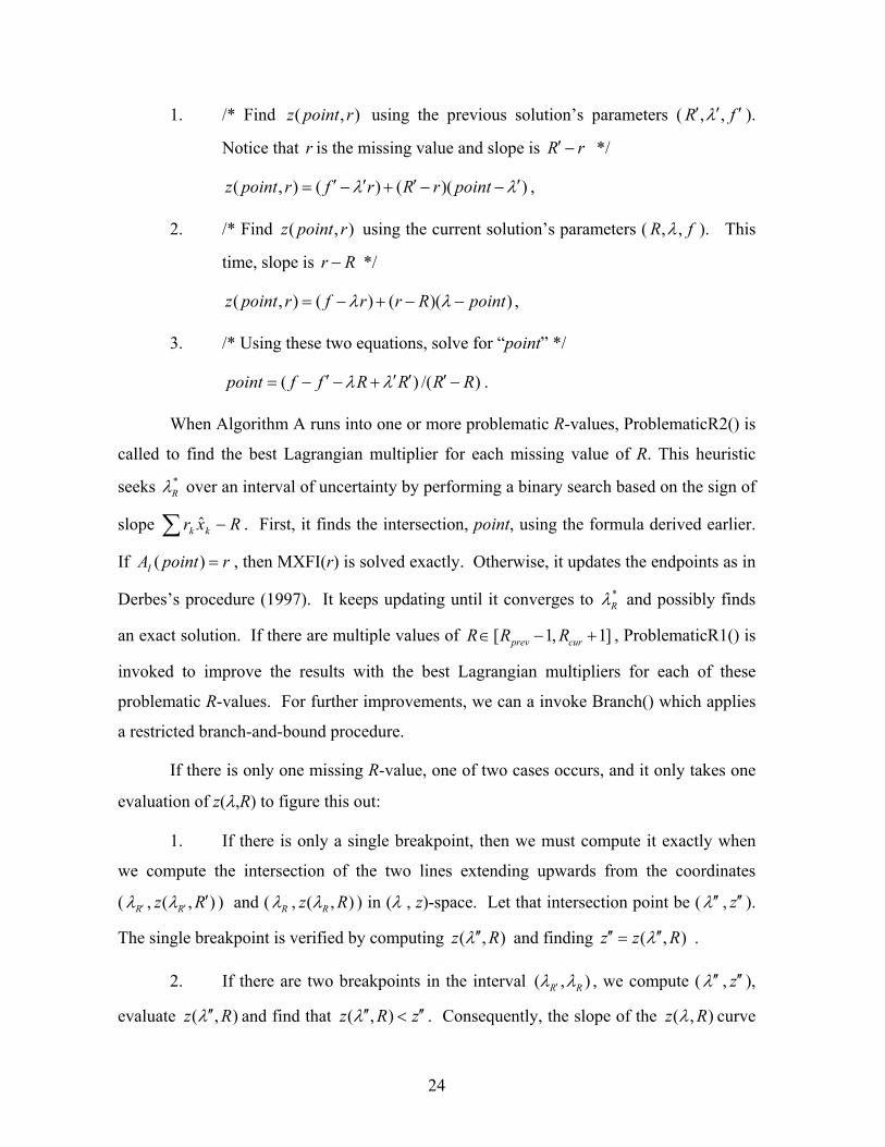
In our heuristic above, we derive the formula point = ( ) /( )f f R R R Rλ λ′ ′ ′ ′− − + −

in order to find the intersection with the following steps:

24

1. /* Find ( , )z point r using the previous solution’s parameters ( , ,R fλ′ ′ ′ ).

Notice that r is the missing value and slope is R r′ − */

( , ) ( ) ( )( )z point r f r R r pointλ λ′ ′ ′ ′= − + − − ,

2. /* Find ( , )z point r using the current solution’s parameters ( , ,R fλ ). This

time, slope is r R− */

( , ) ( ) ( )( )z point r f r r R pointλ λ= − + − − ,

3. /* Using these two equations, solve for “point” */

( ) /( )point f f R R R Rλ λ′ ′ ′ ′= − − + − .

When Algorithm A runs into one or more problematic R-values, ProblematicR2() is

called to find the best Lagrangian multiplier for each missing value of R. This heuristic

seeks *Rλ over an interval of uncertainty by performing a binary search based on the sign of

slope ∑ − Rxr kk ˆ . First, it finds the intersection, point, using the formula derived earlier.

If ( )IA point r= , then MXFI(r) is solved exactly. Otherwise, it updates the endpoints as in

Derbes’s procedure (1997). It keeps updating until it converges to *Rλ and possibly finds

an exact solution. If there are multiple values of [ 1, 1]prev curR R R∈ − + , ProblematicR1() is

invoked to improve the results with the best Lagrangian multipliers for each of these

problematic R-values. For further improvements, we can a invoke Branch() which applies

a restricted branch-and-bound procedure.

If there is only one missing R-value, one of two cases occurs, and it only takes one

evaluation of z(λ,R) to figure this out:

1. If there is only a single breakpoint, then we must compute it exactly when

we compute the intersection of the two lines extending upwards from the coordinates

( Rλ ′ , ( , )Rz Rλ ′ ′ ) and ( Rλ , ( , )Rz Rλ ) in (λ , z)-space. Let that intersection point be (λ′′ , z′′ ).

The single breakpoint is verified by computing ( , )z Rλ′′ and finding ( , )z z Rλ′′ ′′= .

2. If there are two breakpoints in the interval ( , )R Rλ λ′ , we compute (λ′′ , z′′),

evaluate ( , )z Rλ′′ and find that ( , )z R zλ′′ ′′< . Consequently, the slope of the ( , )z Rλ curve

25

must lie strictly between one and negative one. Since the slope can only change by integer

amounts, we have found a portion of the curve where the slope is zero and will,

consequently, have solved MXFI(R) optimally.

If there are sequential problematic R-values, there are three possibilities:

1. There may not be an exact solution for any of the problematic R-values. In

this case, the procedure finds *Rλ and then ProblematicR1() is called with updated

parameters to find the best LB. In fact, λ and λ′ computed earlier by Algorithm A are at

some ku . However, when computed by ProblematicR2(), either λ or λ′ becomes the best

Lagrangian multiplier, which helps improve LB for these problematic R-values. To invoke

Branch(), we use the following idea: When there are more than one problematic R-values at

one breakpoint, the best Lagrangian multiplier is the same for all these values. In other

words, for [ 1, 1]R R R′∈ − + , * * *1 2 1R R Rλ λ λ+ + −= = = . Therefore, we use only one of them

with a slight perturbation, *1rλ ε+ − , to invoke Branch(), where *

1| ( ) |I r prevA R Rλ ε+ ′− = = .

2. The interval of uncertainty might yield an exact solution for some of the

problematic R-values. If it does, then the procedure prints out the results of those values,

and prevR and curR establish new endpoints for the problematic R-values. If 1prev curR R− > ,

ProblematicR1() and/or Branch() can be invoked to find a feasible solution and optimality

gap for problematic [ 1, 1]cur prevR R R∈ + − as explained in the previous paragraph. Since

( )prevRIA and/or ( )curR

IA might change for the problematic [ 1, 1]cur prevR R R∈ + − , not only LB

but also UB are computed by ProblematicR1().

3. The procedure might solve MXFI(R) exactly for all missing R-values in the

sequence. In our tests in Chapter IV, we observe this in two instances out of 10 test

problems.

D. RESTRICTED BRANCH-AND-BOUND

Using procedure ProblematicR2() to solve MXFI, we may be able to reduce the

optimality gap by a substantial amount or solve MXFI exactly, for certain values of R.

26

However, there might be some problematic R-values for which the optimality gap is still

large. For these R-values, we can resort to branch-and-bound.

The usual idea of the branch-and-bound in the setting of integer programming is the

following: Assume that we have a feasible, binary integer-programming problem (BIP).

We can solve the BIP as a linear program (LP) (i.e., the linear-programming relaxation of

BIP) by ignoring the integer restrictions. If the LP optimal solution contains only binary-

valued variables we have solved the BIP. Otherwise, we select a fractional variable, say

kx , and branch on it. That is, we create two new LPs, LP1 and LP2, by introducing the

constraints 0kx = and 1kx = , respectively. An optimal solution to the original problem is

contained in the feasible region to at least one of these two problems. Next, we select one

of the problems, say LP1, solve it (the LP relaxation that is), and evaluate its objective. If

the objective is no better than the value of some incumbent integer solution (which we

obtained heuristically, say), then that problem is fathomed by bounds. If the problem is

infeasible, it is fathomed by infeasibility. If the solution is integer then we have fathomed

by integrality (and we save this solution as the incumbent if it is better than any we have

seen before). If none of those cases occur for LP1, we select a fractional variable and

recursively branch on it. Branch and bound stops when all nodes are fathomed: The best

solution found is optimal. (Note that some subproblems that have not been solved may be

fathomed using information from other subproblem solutions. For instance, if an optimal

integer solution to LP1 is found and its objective value equals that of LP, then LP2 is

implicitly fathomed by bounding.)

But in our scheme for solving MXFI, there are no fractional values. Thus, we need

a different partitioning scheme. We will base the partition on, essentially, setting 0=kx or

1=kx for ( )Ik A λ′∈ , where ( )IA Rλ′ > . In this case, “forcing arc k into the solution” is

equivalent to setting 1=kx and “forcing arc k out of the solution” corresponds to setting

0=kx . And, we will consider a node fathomed if, at that node:

1. | |IA R= (equivalent to being fathomed by integrality; an optimal solution to

the subproblem has been found), and

27

2. ( , )z R UBλ > . (Fathomed by bounding.)

If we use this technique in our problem, our enumeration tree might look like the

following, given ( )IA λ′ = {m, n, r} :

Figure 4. Sample Enumeration Tree for R = 1. Solutions are given next to nodes in curly braces and the branching decision is next to the branches: “ The initial solution at the root node at level 0 is {m, n, r}. “ m ” and “m” represent the exclusion and inclusion of arc m, respectively. Note that none of the nodes are fathomed in this sample enumeration tree.

In Figure 4, every time we force an arc in, we obtain the same solution. For

example, when arc m is included for the solution at Level 1, we get the solution {m, n, r}

from Level 0. But, it is unnecessary to consider a branch with {m, n, r}, because we have

already evaluated this solution. So, we modify the procedure as follows:

v v n

mm

{ , , }m n r { , }v y

{ , , }m n r (Level 0)

(Level 1)

(Level 2)

n

28

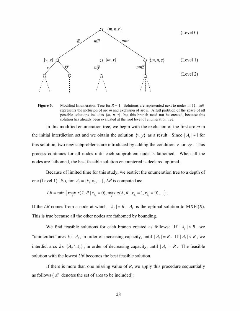
Figure 5. Modified Enumeration Tree for R = 1. Solutions are represented next to nodes in {}. nm represents the inclusion of arc m and exclusion of arc n. A full partition of the space of all possible solutions includes {m, n, r}, but this branch need not be created, because this solution has already been evaluated at the root level of enumeration tree.

In this modified enumeration tree, we begin with the exclusion of the first arc m in

the initial interdiction set and we obtain the solution },{ yv as a result. Since | | 1IA ≠ for

this solution, two new subproblems are introduced by adding the condition v or vy . This

process continues for all nodes until each subproblem node is fathomed. When all the

nodes are fathomed, the best feasible solution encountered is declared optimal.

Because of limited time for this study, we restrict the enumeration tree to a depth of

one (Level 1). So, for 1 2{ , , }IA k k= … , LB is computed as:

1 1 2min max ( , | 0), max ( , | 1, 0),{ }k k kLB z R x z R x x

λ λλ λ= = = = … .

If the LB comes from a node at which | |IA R= , IA is the optimal solution to MXFI(R).

This is true because all the other nodes are fathomed by bounding.

We find feasible solutions for each branch created as follows: If | |IA R> , we

“uninterdict” arcs Ik A∈ , in order of increasing capacity, until | |IA R= . If | |IA R< , we

interdict arcs { \ }C Ik A A∈ , in order of decreasing capacity, until | |IA R= . The feasible

solution with the lowest UB becomes the best feasible solution.

If there is more than one missing value of R, we apply this procedure sequentially

as follows ( A+ denotes the set of arcs to be included):

my

mnz

{ , , }m n r

m mn

{ , }v y

v vy { , }m y

mnz{ , , }m n z

(Level 0)

(Level 1)

(Level 2)

29

Procedure Branch( R′ , R, λ , ( )RIA ′ , UB(r))

Input: Network G= (N, A), source node s, sink node t, R current R-value correctly solved, R′ previous R-value correctly solved (R′ > R + 1),

λ value of parameter such as *1Rλ λ ε+= − ,

( )RIA ′ interdiction set that corresponds to ˆ( )R′x ,

UB(R) feasible objective value for ˆ ( )Rx .

Output: ˆ ( )Rx feasible (possibly optimal) solution for MXFI(R), ( )R

IA interdiction set that corresponds to ˆ ( )Rx , LB(R) possibly improved lower bound on optimal objective value z(R), ( )UB R possibly improved feasible objective value for ˆ ( )Rx , absGap(R) for problematic R: absolute optimality gap UB(R) − LB(R), relGap(R) for problematic R: relative optimality gap 100×absGap(R)/LB(R).

{

for (r = R′ – 1 to R + 1) { /* Solve for all missing values of R */

min{ , }k k R ku u rλ ′′ ← for all Ak ∈ ; /* adjust arc capacities */

( )LB r ←∞ ;

A+ ← Ø; /* This will be the set of arcs forced into the solution */

for (a = 1 to r + 1) { /* Include and exclude the arcs in AI(r) */

Let k be the ath arc in AI( r );

If ( k ∉ A+ ) { /* if k is not already forced in */

ku′ ← ku ; /* forces arc k out of the cut, i.e., sets ˆ 0kx = */

}


ÎA ← {k ∈ AC | ku′ = λ };

Î IA A A+← ∪ ;

ˆ ˆ1 ; 0 \ ;k I k Ix k A x k A A← ∀ ∈ ← ∀ ∈

ˆ| |local I RUB f A λ ′← − ;

30

/* Find a feasible solution */

if ( | |IA r> ) {

for ( | |IA down to r ) {

min arg minI

kk Ak u

∈← ;

minlocal local kUB UB u← + ;

min{ }I IA A k← − ;

ˆ 0kx ← ;

}

}

/* Find a feasible solution */

if ( | |IA r< ) {

for ( r down to | |IA ) {

max { / }arg max

C Ikk A A

k u∈

← ;

maxlocal local kUB UB u← − ;

max{ }I IA A k← + ;

ˆ 1kx ← ;

}

}

( 1)local RLB f r aλ ′= − − + ;

( ) min{ ( ), }localLB r LB r LB=

( ) min{ ( ), }localUB r UB r UB=

0;ku′ = /* Set 1kx = in the following subproblems */

{ };A A k+ +← ∪

}

absGap ( )r ← UB ( )r − LB ( )r ;

relGap ( )r ← 100×absGap ( )r /LB ( )r ;

print (“ For problematic R = ”, r, “the approximate soln. to MXFI(R) is: ”);

31

print ( x̂ , IA ,UB ( )r , LB ( )r , absGap ( )r , relGap ( )r ); }

}

In this procedure, we force an arc out of a solution by taking its capacity back to its

original level, k Ru λ ′> . This ensures that it will never be seen as interdicted since ÎA ≡ { k

∈ AC | ku′ = Rλ ′}. “Forcing in” is accomplished by setting 0ku′ = , which means that arc k is

destroyed and cannot be used.

Although it is not shown in the pseudo-code for simplicity, if | |IA r≠ , we keep

solving max-flow problems for kuλ ∈ to find | ( ) |IA rλ = . If it doesn’t exist, then we

find minλ and maxλ such that min max| ( ) | | ( ) |I IA r Aλ λ< < . After finding these values, we

compute localLB the way it is computed in ProblematicR1( ):

max max min minmax{( ( ) ( 1)), ( ( ) ( 1))}localLB f r a f r aλ λ λ λ= − − + − − + .

If we find LB UB= , then MXFI is solved exactly for that value of R. Otherwise, we

may obtain an improved LB and/or UB, which decreases the optimality gap.

32


33

IV. COMPUTATIONAL RESULTS

In this chapter, we describe the design of test problems, and provide computational

results for our Lagrangian-based procedures to solve MXFI.

A. TEST NETWORK DESIGN

We use grid networks to test our procedures. “NET a b× ” denotes such a network,

where a is the number of nodes on the horizontal axis and b is the number of nodes on the

vertical axis. The number of nodes in a grid network is | | 2N ab= + , and the number of

arcs is | | (5 4) 5 6A a b b= − − + . A representation of a small network is given in Figure 6:

Figure 6. NET 3 3× . Arc capacities ku and resources kr are not shown in this network. The source node and sink node are numbered 1 and 2, respectively.

As shown in Figure 6, all horizontal arcs lie in the direction of “west to east,” and

diagonal arcs are oriented in the southeast and northeast directions. There are also vertical

arcs, north-pointing and south-pointing, between adjacent nodes in a column of nodes;

although these are omitted in the first and last columns, where they would be superfluous

for maximizing flow. Arcs going out of the source node and going into the sink node have

infinite capacity and cannot be interdicted. (In fact, uninterdictable arcs have 999kr = ,

1

3

4

5 8

7

6 9

10

11

2

34

which effectively makes them uninterdictable.) All the other arcs are interdictable. Finite

arc capacities ku are drawn from a discrete uniform distribution with range [1,50].

We use the network generator written in C by Derbes (1997) and modify it for

different networks. The network files generated by this program provide the following

information about the structure of the network: number of nodes, number of arcs, source

and sink nodes. Also, each arc k receives a capacity ku , cost of repair kc , resource needed

to interdict kr , and “reparability” kp . However, we use only ku and kr in our tests.

B. RESULTS

We use six different grid networks for testing. The smallest one, NET 5 5× , has 27

nodes and 86 arcs. The largest one, NET 20 20× , has 402 nodes and 1826 arcs. All tests

are performed on a 533 MHz Pentium III personal computer with 192 MB of RAM and

running the Microsoft Windows XP Professional operating system. All programs are

written in the Java 1.3 programming language.

We use three different methods to test the effectiveness of our Lagrangian-based

procedures. Each method uses Algorithm A with a different procedure or procedures.

Procedure ProblematicR1() is the heuristic that Bingol (2001) uses to find a feasible

solution, and a lower bound on *( , )Rz Rλ . We use ProblematicR2() to find the best

Lagrangian multipliers. The procedure Branch() applies the restricted branch-and-bound

technique introduced in Chapter III. Method 1 uses ProblematicR1() integrated into

Algorithm A; this is the technique Bingol (2001) analyzes. In particular, every time

Algorithm A runs into a contiguous set of problematic R-values, ProblematicR1() is called

to find UB and LB for each. Method 2 works the same way, but ProblematicR2() is

invoked to find *Rλ for problematic R-values before parameters are passed on to

ProblematicR1() which is, in this case, only used to find feasible solution. Furthermore,

the indicated call to Branch() inside of ProblematicR2() is not made. Method 3 invokes

procedure ProblematicR2() exactly as stated in the text, i.e., with a call to Branch() if a

positive gap remains.

35

Since we are really only concerned with problematic R-values, the tables only

present: the problematic values R, total run-times, upper bounds ( )z R , lower bounds

( , )z Rλ , absolute gaps “absGap,” and relative gaps “relGap.” Tables also include the

uninterdicted maximum flow value *f .

Table 1 shows results for Method 1. Although all absolute gaps are small, relative

gaps can be as large as 25.0% when the divisor ( , )z Rλ is small. Each network that we

have tested has yielded one or more problematic values. Run-times are small, the largest

one being 31.5 cpu seconds.

Table 2 exhibits results for Method 2 using the same networks. Since the best

Lagrangian mulitiplier is not necessarily an integer, *( , )Rz Rλ might have fractional values.

“absGap” and “relGap” are the results computed with these fractional values. However,

optimal objective values must be integral, so it makes sense to round *( , )Rz Rλ up to the

nearest integer. Thus, “ absGap ” and “ relGap ” denote absolute and relative gaps

computed after this rounding. Of 36 problematic R-values found with Method 1, Method 2

solves 16 exactly. The largest remaining relative gap is 14.3% for 51R = in NET 20 20× .

Run-times increase only slightly for the networks that have a few problematic R-values. If

ProblematicR2() is invoked many times, the increase is about 25%.

Table 3 presents the results of Method 3 which invokes procedure Branch(). We

only pass on to this procedure the problematic R-values remaining after Method 2. With

this method, the number of remaining problematic R-values values goes down to four for

NET 20 20× . The largest relative gap drops to 7.1%, since a better feasible solution is

found by Branch(). There can be, unfortunately, a drastic increase in run-time; for

example, the run time increases from 31.5 seconds to 4013.7 seconds for NET 20 20× .

To explore the effectiveness of these methods further, we use NET 8 15× with

restricted capacities. There are four types of restricted capacities, denoted 16[1,2], 8[1,4],

4[1,8], 2[1,16]: The notation “ [1, ]p q ” indicates that the random capacities are drawn

uniformly from the set { , 2 , ,p p qp… }. Bingol (2001) finds problem instances like these,

with few distinct capacities, to be particularly difficult. That is, they tend to yield large

36

optimality gaps. We apply the same three methods as before: Table 4 includes only

problematic R-values with relative gaps higher than 5% remaining after Method 1.

We start with a total of 16 problematic values from Method 1. The largest relative

gap from Method 1 is 20%. By using Method 2, the number of problematic R-values goes

down to eight, with the largest gap being 6.1%. Four of these problematic values are

solved exactly by Method 3. However, there is no improvement in the relative gaps of the

remaining four.

37

G = (N, A ) Run Time (cpu sec.)

Problematic R -Values

6 55 53 2 3.8%2 159 152 7 4.6%

17 18 17 1 5.9%16 29 27 2 7.4%15 39 37 2 5.4%14 48 47 1 2.1%

6 202 200 2 1.0%5 228 227 1 0.4%

NET 8 12 690 [1,34] 1.0 15 189 188 1 0.5%40 5 4 1 25.0%39 7 6 1 16.7%34 27 26 1 3.8%24 146 145 1 0.7%23 165 162 3 1.9%22 181 180 1 0.6%17 279 278 1 0.4%

6 590 588 2 0.3%38 11 10 1 10.0%10 431 430 1 0.2%

9 463 462 1 0.2%3 686 684 2 0.3%

53 8 7 1 14.3%51 16 14 2 14.3%50 19 18 1 5.6%41 83 80 3 3.8%40 93 89 4 4.5%39 101 98 3 3.1%38 110 108 2 1.9%37 119 118 1 0.8%32 175 174 1 0.6%17 508 507 1 0.2%16 542 541 1 0.2%15 576 575 1 0.2%14 611 609 2 0.3%11 712 711 1 0.1%

7 859 858 1 0.1%

31.5NET 20 20 1173 [1,58]

[1,43] 7.5

NET 8 15 841 [1,43] 1.9

NET 15 15 878

NET 8 8 416 [1,22] 0.4

NET 5 5 234 [1,13] 0.1

),( Rz λ*f

×

×

×

×

×

×

R1absGap 1relGap( )z R

Table 1. Test Results for Method 1. This is essentially Bingol’s procedure (Bingol 2001) which uses

Algorithm A with ProblematicR1(), but not ProblematicR2() or Branch(). f ∗ shows maximum flow without interdiction. The column labeled “R” gives the range of interdiction resource levels tested; he maximum flow goes to 0 when R equals the second of the two numbers. Run times cover the whole procedure, but only problematic R-values remaining after the procedure is run are shown. ( )z R is the upper bound obtained from the best solution with ProblematicR1() and ( , )z Rλ is the largest value of Lagrangian function

obtained from MXFI-LRD. ( , )z Rλ is always integer since kuλ = for k A∈ .

“ 1absGap ” is ( ) ( , )z R z Rλ− and “ 1relGap ” is 1100 absGap / ( , )z Rλ× .

38


Problematic R -Values absGap relGap

6 55 53.5 1.5 2.8% 54 1 1.9% 3.8%2 159 152.5 6.5 4.3% 153 6 3.9% 4.6%

17 18 17.2 0.8 4.7% 18 - - 5.9%16 29 27.4 1.6 5.8% 28 1 3.6% 7.4%15 39 37.6 1.4 3.7% 38 1 2.6% 5.4%14 48 47.8 0.2 0.4% 48 - - 2.1%6 202 200 2.0 1.0% 200 2 1.0% 1.0%5 228 227 1.0 0.4% 227 1 0.4% 0.4%

NET 8 12 690 [1,34] 1.0 15 189 188.5 0.5 0.3% 189 - - 0.5%40 5 4.3 0.7 16.3% 5 - - 25.0%39 7 6.7 0.3 4.5% 7 - - 16.7%34 27 26.5 0.5 1.9% 27 - - 3.8%24 146 145.5 0.5 0.3% 146 - - 0.7%23 165 163 2.0 1.2% 163 2 1.2% 1.9%22 181 180.5 0.5 0.3% 181 - - 0.6%17 279 278.5 0.5 0.2% 279 - - 0.4%6 590 588.5 1.5 0.3% 589 1 0.2% 0.3%

38 11 10.5 0.5 4.8% 11 - - 10.0%10 431 430.3 0.7 0.2% 431 - - 0.2%9 463 462.7 0.3 0.1% 463 - - 0.2%3 686 684.5 1.5 0.2% 685 1 0.1% 0.3%

53 7 7 - - 7 - - 14.3%51 16 14 2.0 14.3% 14 2 14.3% 14.3%50 19 18 1.0 5.6% 18 1 5.6% 5.6%41 83 80.5 2.5 3.1% 81 2 2.5% 3.8%40 93 90 3.0 3.3% 90 3 3.3% 4.5%39 101 99.5 1.5 1.5% 100 1 1.0% 3.1%38 110 109 1.0 0.9% 109 1 0.9% 1.9%37 119 118.5 0.5 0.4% 119 - - 0.8%32 175 174.5 0.5 0.3% 175 - - 0.6%17 508 507.8 0.2 0.0% 508 - - 0.2%16 542 541.5 0.5 0.1% 542 - - 0.2%15 576 575.3 0.7 0.1% 576 - - 0.2%14 609 609 - - 609 - - 0.3%11 712 711.5 0.5 0.1% 712 - - 0.1%7 859 858 1.0 0.1% 858 1 0.1% 0.1%

NET 5 5 234 [1,13] 0.1

NET 8 8 416 [1,22] 0.7

NET 8 15 841 [1,43] 2.3

NET 15 15 878 [1,43] 10.3

NET 20 20 1173 [1,58] 39.3

*( , )Rz Rλ *( , )Rz Rλ *f

×

×

×

×

×

×

2absGapR 2relGap 1relGap( )z R

Table 2. Test Results for Method 2. This method uses Algorithm A and invokes ProblematicR2() and ProblematicR1(). ProblematicR2() finds the best Lagrangian multipliers *

Rλ for problematic R-values, which are then passed on to ProblematicR1() to find feasible

solutions. Since z(R) is integer, *( , )R

z Rλ is a valid lower bound on z(R). “ 2absGap ” is

*( ) ( , )Rz R z Rλ− and “ 2relGap ” is *

2100 absGap / ( , )Rz Rλ× . “ absGap ” is

*( ) ( , )Rz R z Rλ− and “ relGap ” is *100 absGap / ( , )Rz Rλ× . “-“ indicates that MXFI is solved optimally. Only two problematic R-values, R = 53 and R = 14 for NET 20 20× , are

solved exactly before rounding up *( , )Rz Rλ but, overall, more than 50% of the problematic

R-values are solved with rounding. 1relGap is shown for comparison.

39


Problematic R -Values

6 55 55 55 - - 3.8% 1.9%2 159 158 158 1 0.6% 4.6% 3.9%

17 18 18 18 - - 5.9% -16 29 29 29 - - 7.4% 3.6%15 39 39 39 - - 5.4% 2.6%14 48 48 48 - - 2.1% -

6 202 202 202 - - 1.0% 1.0%

5 228 228 228 - - 0.4% 0.4%NET 8 12 690 [1,34] 4.4 15 189 189 189 - - 0.5% -

40 5 4.3 5 - - 25.0% -39 7 6.7 7 - - 16.7% -34 27 27 27 - - 3.8% -24 146 146 146 - - 0.7% -23 165 165 165 - - 1.9% 1.2%22 181 181 181 - - 0.6% -17 279 279 279 - - 0.4% -

6 590 590 590 - - 0.3% 0.2%38 11 11 11 - - 10.0% -10 431 431 431 - - 0.2% -

9 463 463 463 - - 0.2% -3 686 686 686 - - 0.3% 0.1%

51 15 14 14 1 7.1% 14.3% 14.3%50 19 18 18 1 5.6% 5.6% 5.6%41 83 83 83 - - 3.8% 2.5%40 93 92 92 1 1.1% 4.5% 3.3%39 101 101 101 - - 3.1% 1.0%38 110 110 110 - - 1.9% 0.9%37 119 119 119 - - 0.8% -32 175 174.5 175 - - 0.6% -17 508 508 508 - - 0.2% -16 542 542 542 - - 0.2% -15 576 576 576 - - 0.2% -11 712 712 712 - - 0.1% -

7 859 859 859 - - 0.1% 0.1%

NET 5 5 234 [1,13] 0.2

25.2

NET 8 8 416 [1,22] 7.0

NET 8 15 841 [1,43]

NET 15 15 878 [1,43] 96.0

NET 20 20 1173 [1,58] 4013.7

L B

×

×

×

×

×

*f L B

×

3absGap 3relGap 1relGap 2relGapR ( )z R

Table 3. Test Results from Method 3. Method 3 is essentially Method 2 except that Branch() is invoked for problematic R-values that Method 2 cannot resolve. minLB =

1 1 2{max ( , | 0), max ( , | 1, 0), }k k kz R x z R x x

λ λλ λ= = = … . “ 3absGap ” is ( )z LBλ − and

“ 3relGap ” is 3100 absGap / LB × . Absolute and relative gaps computed with fractional values are not shown in this table. 12 problematic R-values out of the 16 remaining after Method 2 are solved exactly by Method 3. UB for R = 51 of NET 20 20× drops from 16 to 15, because a better feasible solution is found by Branch(). 1relGap and 2relGap are also shown in the table for comparison.

40

G =(N , A ) Problematic R -Values

24 320 304 5.3% 304 304 - - - -23 352 320 10.0% 320 320 - - - -22 384 336 14.3% 336 336 - - - -21 400 352 13.6% 352 352 - - - -20 416 368 13.0% 368 368 - - - -19 432 384 12.5% 400 394 1.5% 400 394 1.5%18 448 400 12.0% 432 420 2.9% 432 420 2.9%17 464 432 7.4% 464 446 4.0% 464 446 4.0%31 104 96 8.3% 96 96 - - - -30 120 104 15.4% 112 110 1.8% 112 112 -29 128 120 6.7% 128 123 4.1% 128 123 4.1%38 240 200 20.0% 200 200 - - - -37 280 240 16.7% 240 240 - - - -35 280 260 7.7% 280 264 6.1% 280 280 -34 340 320 6.3% 340 329 3.3% 340 340 -33 400 380 5.3% 400 393 1.8% 400 400 -

16[1,2]

8[1,4]

4[1,8]

2[1,16]

2relGap 3relGap1relGap ( )z R ( )z R( )z R L B *( , )Rz Rλ ),( Rz λ

Table 4. Comparative Test Results for NET 8 15× with Restricted Arc Capacities. “Methods” are defined in the text. Arc capacities denoted [1, ]p q

are drawn from the set { , 2 , ,p p qp… }. “ 1relGap , 2relGap , and 3relGap ” are the relative gaps obtained from Method 1, 2 and 3, respectively. Only R-values with relative gaps remaining greater than 5% after Method 1 are shown in this table. 50% of problematic R-values are solved exactly by Method 2, and 50% of those remaining are then solved by Method 3. Notice that UB for R = 30 of the network with arc capacities 8[1,4] has dropped from 120 to 112, because R=31 is solved exactly by Method 2, and this makes it possible to find a better feasible solution for R = 30.

Method 3Method 1 Method 2

41

V. CONCLUSIONS AND FURTHER RESEARCH

A. SUMMARY

The maximum-flow network-interdiction problem (MXFI) arises when an

“interdictor” uses limited interdiction resources to restrict an adversary’s use of a network.

Conceptually, the interdictor destroys arcs to minimize the maximum flow that the

adversary, or “network user,” can achieve through the network. In this study, we have

explored new Lagrangian-relaxation techniques for solving MXFI for all values of

interdiction resource R in a specified range. We assume that one unit of resource is

required to interdict an arc, so we only deal with integer values of R.

MXFI can be solved by means of integer programming, but this approach is slow.

Bingol (2001) modifies the Lagrangian-relaxation technique developed by Derbes (1997)

to solve MXFI for all R ∈ [1, min| |A ], where minA denotes a minimum cardinality cut

consisting of only interdictable arcs. The Lagrangian-relaxation technique solves a

sequence of max-flow problems with related arc capacities, and is therefore quite efficient.

Let ( )z R denote the optimal objective value to MXFI for a given R, and let

( , )z Rλ denote the Lagrangian lower bound on ( )z R given Lagrangian multiplier λ .

Essentially, Bingol (2001) evaluates ( , )z Rλ simultaneously for all R, but only for values

of λ equal to perturbed arc capacities. We follow this procedure—the range of λ is

correct—but, when ( , ) ( )z R z Rλ < for *Rλ = argmax ( , )z R

λλ , where ( )z R is the objective-

function value for the best feasible solution found. This is accomplished with a search

technique based on the slope of ( , )z Rλ with respect to λ . For most test problems, we can

decrease the optimality gap for “problematic R-values” by approximately 50%. A value of

R is “problematic” if Bingol’s procedure leaves ( , ) ( )z R z Rλ < . Although this approach

focuses on tightening lower bounds, it is also finds better feasible solutions on occasion,

and sometimes proves optimality of the best solution. However, some large optimality

gaps may remain.

42

We tackle the remaining problematic R-values with a modified branch-and-bound

procedure. This procedure uses a partition based on the best interdiction set found,

1 2{ , , , }I LA k k k= … . In particular, we solve 1 2

max ( , | 1, 0), ,k kz R x xλ

λ = = …

1 2max ( , | 1, 1,k kz R x x

λλ = = ,…

11, 0)

L Lk kx x−= = . ( max ( , | 1 )k Iz R x k A

λλ = ∀ ∈ is already

solved.) The minimum lower bound from these problems is a lower bound on the optimal

solution. This partitioning scheme can be applied recursively to solve MXFI exactly for a

given R, but we have only implemented a single application of the partition. That is, we

have limited the enumeration tree of this method to one level below the root. Using this

technique, we may find a lower bound which equals the upper bound obtained from the

best feasible solution. In this case, MXFI is solved. In our tests, we have solved

approximately 70% of the problematic R-values that remain after applying the first

technique. But, this procedure runs slowly because of the need to solve many max-flow

problems, so it is best used only when large optimality gaps are encountered.

Having used these two techniques together, we have been able to solve MXFI either

exactly or with small optimality gaps for most of the problematic R-values encountered.

But, we still cannot guarantee an exact solution or a small optimality gap.

B. FURTHER RESEARCH

In this thesis, we have used a restricted modified branch-and-bound procedure that

explores the enumeration tree only one level below the root. That is why some problematic

R-values still remain. A fully recursive implementation of the branch-and-bound algorithm

will solve MXFI exactly, at least in theory. Even the restricted branch-and-bound

procedure becomes slow because of the need to solve many max-flow problems. Thus, a

fully recursive procedure based on this methodology would be even slower. To make such

a procedure reasonably efficient, a faster maximum-flow algorithm should be used and

techniques for reoptimizing related maximum-flow problems should be explored.

For the sake of simplicity, we have assumed that that 1kr = for all interdictable arcs

k. That is, one unit of resource is needed to interdict any interdictable arc. Allowing

43

1kr > (but still integer) will make the problem harder. In this case, a complete branch-and-

bound procedure would become more important to possess.

We have assumed that grid networks are adequate representatives for real-world

networks, so we have performed our tests on these networks. However, we are uncertain

how well these procedures will perform on actual networks. Obviously, future research

should apply these techniques to more realistic networks.

44


45

LIST OF REFERENCES

Ahuja, R.K., Magnanti, T.L., and Orlin, J. B., Network Flows, Prentice Hall, New Jersey, 1993, pp. 601-603.

Akgun, I., “The K-Group Maximum-Flow Network Interdiction Problem,” Master’s Thesis, Naval Postgraduate School, Monterey, California, March 2000.

Balcioglu, A., “An Algorithm for Enumerating the Near-Minimum Weight s-t Cuts of a Graph,” Master’s Thesis, Naval Postgraduate School, Monterey, California, December 2000.

Bingol, L., “A Lagrangian Heuristic for Solving a Network Interdiction Problem,” Master’s Thesis, Naval Postgraduate School, Monterey, California, December 2001.

Cormican, K.J., “Computational Methods for Deterministic and Stochastic Network Interdiction Problems,” Master’s Thesis, Naval Postgraduate School, Monterey, California, March 1995.

Cormican, K.J., Morton, D.P., and Wood, R.K., “Stochastic Network Interdiction,” Operations Research, Vol. 46, pp. 184-197, 1998.

Derbes, H.D., “Efficiently Interdicting a Time-Expanded Transshipment Network,” Master’s Thesis, Naval Postgraduate School, Monterey, California, September 1997.

Edmonds, J., and Karp, R.M., “Theoretical Improvements in Algorithmic Efficiency for Network flow Problems,” Journal of the Association for Computing Machinery, Vol. 19, No. 2, April 1972.

Ford, L.R., Jr., and Fulkerson, D.R., “Maximal Flow through a Network,” Canadian Journal of Mathematics, 1956.

Ghare, P.M., Montgomery, D.C., and Turner, W.C., “Optimal Interdiction Policy for a Flow Network,” Naval Research Logistics Quarterly, Vol. 18, pp. 37-45, 1971.

Golden, B., “A Problem in Network Interdiction,” Naval Research Logistics Quarterly, Vol. 25, pp. 711-713, 1978.

Israeli, E., “System Interdiction and Defense,” Doctoral Dissertation, Naval Postgraduate School, Monterey, California, March 1999.

Israeli, E., and Wood, R.K., “Shortest Path Network Interdiction,” Networks, to appear.

Lubore, S.H., Ratliff, H.D., and Sicilia, G.T., “Finding the n most Vital Links in Flow Networks,” Management Science, Vol. 21, No. 5, 1975.

McMasters, A.W., and Mustin, T.M., “Optimal Interdiction of a Supply Network,” Naval Research Logistics Quarterly, Vol. 17, pp. 261-268, 1970.

Morton, D., “Stochastic Network Interdiction of Nuclear Material Smuggling,” Systems and Industrial Engineering Seminar, September 2001.

Steinrauf, R.L., “Network Interdiction Models,” Master’s Thesis, Naval Postgraduate School, Monterey, California, September 1991.

46

Taha, H.A., Operations Research, 6th ed., Prentice Hall, New Jersey, 1997, pp. 385-390.

Wevley, C.M., “The Quickest Path Network Interdiction Problem,” Master’s Thesis, Naval Postgraduate School, Monterey, California, March 1999.

Whiteman, P.S., “Improving Single Strike Effectiveness for Network Interdiction,” Military Operations Research, Vol. 4, pp.15-30, 1999.

Wollmer, R.D., “Removing Arcs from a Network,” Operations Research, Vol. 12, pp. 807-1076, 1964.

Wollmer, R.D., “Algorithm for Targeting Strikes in a Lines-of-Communication Network,” Operations Research, Vol. 18, pp.497-515, 1970.

Wood, R.K., ”Deterministic Network Interdiction,” Mathematical and Computer Modeling, Vol. 17, No. 2, pp. 1-18, 1993.

47

INITIAL DISTRIBUTION LIST

1. Defense Technical Information Center Ft. Belvoir, VA

2. Dudley Knox Library Naval Postgraduate School Monterey, CA

3. Professor R. Kevin Wood Department of Operations Research, Code OR/Wd Naval Postgraduate School Monterey, CA

4. LCDR Kelly J. Cormican Department of Operations Research, Code OR/CK Naval Postgraduate School Monterey, CA

5. Kara Kuvvetleri Komutanligi Kutuphane Bakanliklar, Ankara, TURKEY

6. Kara Harp Okulu Komutanligi Kutuphane Tuzla, Istanbul, TURKEY

7. Bilkent Universitesi Kutuphanesi Bilkent, Ankara, TURKEY

8. Orta Dogu Teknik Universitesi Kutuphanesi Balgat, Ankara, TURKEY

9. Bogazici Universitesi Kutuphanesi Bebek, Istanbul, TURKEY

10. Top. Utgm. Adnan Uygun Kara Kuvvetleri Komutanligi Bakanliklar, Ankara, TURKEY

Documents

Author(s) Uygun, Adnan Title Monterey, California. Naval