Author(s) Smith, Phillip. Title The uses of a polarimetric

This document was downloaded on May 04, 2015 at 23:42:35

Author(s) Smith, Phillip.

Title The uses of a polarimetric camera

Publisher Monterey California. Naval Postgraduate School

Issue Date 2008-09

URL http://hdl.handle.net/10945/3972

NAVAL

POSTGRADUATE SCHOOL

MONTEREY, CALIFORNIA

THESIS

Approved for public release; distribution is unlimited

THE USES OF A POLARIMETRIC CAMERA

by

Phillip Smith

September 2008

Thesis Advisor: R. C. Olsen Second Reader: R. Harkins

THIS PAGE INTENTIONALLY LEFT BLANK

i

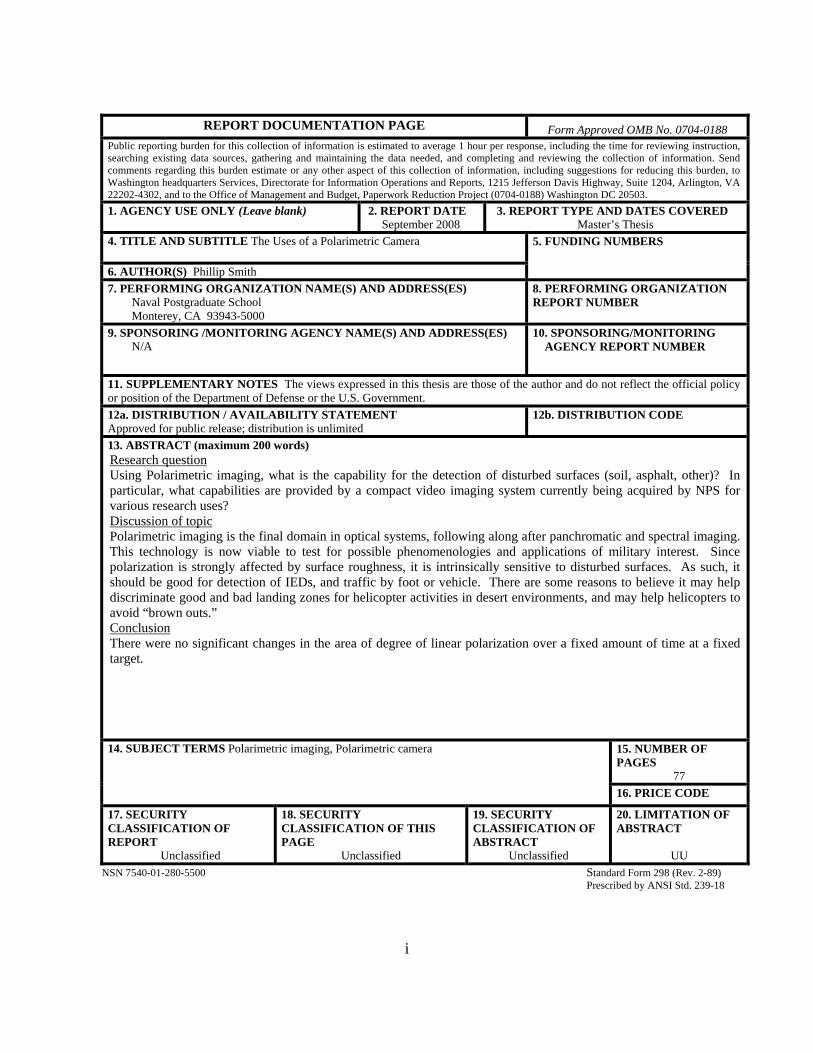
REPORT DOCUMENTATION PAGE Form Approved OMB No. 0704-0188

Public reporting burden for this collection of information is estimated to average 1 hour per response, including the time for reviewing instruction, searching existing data sources, gathering and maintaining the data needed, and completing and reviewing the collection of information. Send comments regarding this burden estimate or any other aspect of this collection of information, including suggestions for reducing this burden, to Washington headquarters Services, Directorate for Information Operations and Reports, 1215 Jefferson Davis Highway, Suite 1204, Arlington, VA 22202-4302, and to the Office of Management and Budget, Paperwork Reduction Project (0704-0188) Washington DC 20503. 1. AGENCY USE ONLY (Leave blank)

2. REPORT DATE September 2008

3. REPORT TYPE AND DATES COVERED Master’s Thesis

4. TITLE AND SUBTITLE The Uses of a Polarimetric Camera 6. AUTHOR(S) Phillip Smith

5. FUNDING NUMBERS

7. PERFORMING ORGANIZATION NAME(S) AND ADDRESS(ES) Naval Postgraduate School Monterey, CA 93943-5000

8. PERFORMING ORGANIZATION REPORT NUMBER

9. SPONSORING /MONITORING AGENCY NAME(S) AND ADDRESS(ES) N/A

10. SPONSORING/MONITORING AGENCY REPORT NUMBER

11. SUPPLEMENTARY NOTES The views expressed in this thesis are those of the author and do not reflect the official policy or position of the Department of Defense or the U.S. Government. 12a. DISTRIBUTION / AVAILABILITY STATEMENT Approved for public release; distribution is unlimited

12b. DISTRIBUTION CODE

13. ABSTRACT (maximum 200 words) Research question Using Polarimetric imaging, what is the capability for the detection of disturbed surfaces (soil, asphalt, other)? In particular, what capabilities are provided by a compact video imaging system currently being acquired by NPS for various research uses? Discussion of topic Polarimetric imaging is the final domain in optical systems, following along after panchromatic and spectral imaging. This technology is now viable to test for possible phenomenologies and applications of military interest. Since polarization is strongly affected by surface roughness, it is intrinsically sensitive to disturbed surfaces. As such, it should be good for detection of IEDs, and traffic by foot or vehicle. There are some reasons to believe it may help discriminate good and bad landing zones for helicopter activities in desert environments, and may help helicopters to avoid “brown outs.” Conclusion There were no significant changes in the area of degree of linear polarization over a fixed amount of time at a fixed target.

15. NUMBER OF PAGES

77

14. SUBJECT TERMS Polarimetric imaging, Polarimetric camera

16. PRICE CODE

17. SECURITY CLASSIFICATION OF REPORT

Unclassified

18. SECURITY CLASSIFICATION OF THIS PAGE

Unclassified

19. SECURITY CLASSIFICATION OF ABSTRACT

Unclassified

20. LIMITATION OF ABSTRACT

UU NSN 7540-01-280-5500 Standard Form 298 (Rev. 2-89) Prescribed by ANSI Std. 239-18

ii


iii

Approved for public release; distribution is unlimited

THE USES OF A POLARIMETRIC CAMERA

Phillip S. Smith Lieutenant, United States Navy

B.A., University of Missouri at Kansas City, 1998

Submitted in partial fulfillment of the requirements for the degree of

MASTER OF SCIENCE IN SPACE SYSTEMS OPERATIONS

from the

NAVAL POSTGRADUATE SCHOOL September 2008

Author: Phillip Smith

Approved by: R. C. Olsen Thesis Advisor

R. Harkins Second Reader

Rudy Panholzer Chairman, Space Systems Academic Group

iv


v

ABSTRACT

Research question

Using Polarimetric imaging, what is the capability for the detection of disturbed

surfaces (soil, asphalt, other)? In particular, what capabilities are provided by a compact

video imaging system currently being acquired by NPS for various research uses?

Discussion of topic

Polarimetric imaging is the final domain in optical systems, following along after

panchromatic and spectral imaging. This technology is now viable to test for possible

phenomenologies and applications of military interest. Since polarization is strongly

affected by surface roughness, it is intrinsically sensitive to disturbed surfaces. As such,

it should be good for detection of IEDs, and traffic by foot or vehicle. There are some

reasons to believe it may help discriminate good and bad landing zones for helicopter

activities in desert environments, and may help helicopters to avoid “brown outs.”

Conclusion

There were no significant changes in the area of degree of linear polarization over

a fixed amount of time at a fixed target.

vi


vii

TABLE OF CONTENTS

I. INTRODUCTION........................................................................................................1 A. WHAT IS LIGHT?..........................................................................................1 B. WHAT IS POLARIZATION?........................................................................2

1. Polarization Filters...............................................................................3 2. Radar.....................................................................................................4

C. APPLICATIONS IN POLARIMETRIC IMAGING...................................5

II. HISTORY AND BASICS OF POLARIMETRY......................................................7 A. POLARIZATION DEFINED .........................................................................7 B. EARLY HISTORY ..........................................................................................8 C. 17TH CENTURY...............................................................................................8 D. EARLY 19TH CENTURY................................................................................9 E. LATER 19TH CENTURY ..............................................................................11 F. 20TH CENTURY.............................................................................................12 G. POLARIZATION BY REFLECTION ........................................................13 H. PERCENT POLARIZATION ......................................................................15 I. UMOV EFFECT ............................................................................................16 J. STOKES VECTORS .....................................................................................16 K. DEGREE OF LINEAR POLARIZATION (DOLP) ..................................17 L. PHASE ANGLE OF POLARIZATION ......................................................18 M. PRESENTATION..........................................................................................18 N. SATURATION...............................................................................................19

III. CAMERA OPERATIONS ........................................................................................21

IV. DATA ANALYSIS AND CONCLUSION ...............................................................31 A. OBSERVATIONS..........................................................................................31 B. CONCLUSION ..............................................................................................46 C. SUMMARY ....................................................................................................47 D. FUTURE APPLICATIONS..........................................................................48

APPENDIX: COMPUTER CODE FOR IMAGE PROCESSING WITH IDL..............49

LIST OF REFERENCES......................................................................................................57

INITIAL DISTRIBUTION LIST .........................................................................................61

viii


ix

LIST OF FIGURES

Figure 1. Visible light region of the electromagnetic spectrum (From NASA, 2007)......1 Figure 2. The vector nature of electromagnetic waves (From Olsen, 2000) (E is in

the x direction, B is in the y direction, and the wave is propagating in the z direction) ............................................................................................................2

Figure 3. How unpolarized light becomes polarized (From The Physics Classroom Tutorial, 2008) ...................................................................................................3

Figure 4. A polarized filter (top) and a non-polarized image (From Meleg, n.d.) ............4 Figure 5. Various locations of land and the different polarization angles that can be

viewed from PALSAR (From Earth Observation Research Center, 1997) .......5 Figure 6. Maxwell’s equations for a transverse wave (From The Citizens’

Compendium, 2008) ..........................................................................................7 Figure 7. Polarized (left) and unpolarized (right) light (From University of Colorado

at Boulder, 2008) ...............................................................................................7 Figure 8. Double refraction (From University of Minnesota, 2008).................................9 Figure 9. Fresnel rhomb retarder (From CeNing Optics, 2006)......................................10 Figure 10. Brewster’s Angle (From Molecular Expressions, 2008) .................................11 Figure 11. Haidinger’s Brush (From Freebase alpha, 2008).............................................11 Figure 12. A light molecule bouncing off an object and heading out in multiple

directions (From Dutch, 1997).........................................................................13 Figure 13. Fresnel Equation (From Olsen, 2007)..............................................................14 Figure 14. Percent of polarization over the land at Shark Bay (From Israel & Duggin,

1992, p. 3) ........................................................................................................15 Figure 15. Percent of polarization over the open ocean and the waters in Shark Bay

(From Israel & Duggin, 1992, p. 2) .................................................................16 Figure 16. Stokes Vectors (From: Cady & Krings, 1998).................................................17 Figure 17. Stokes Vectors, horizontal, vertical, +/- 45, Right/Left-hand and

Unpolarized (From Cady & Krings, 1998) ......................................................18 Figure 18. Image of angle of polarization (From Bossa Nova Tech, 2007)......................20 Figure 19. The Salsa camera (From Bossa Nova Tech, 2007)..........................................21 Figure 20. Drawing of how camera hooks up to computer ...............................................22 Figure 21. Diagram of the inner workings of the SALSA camera (From: Bossa Nova

Tech, 2007) ......................................................................................................23 Figure 22. Salsa camera with computer setup looking south toward California Pacific

Highway 1........................................................................................................24 Figure 23. Front Panel and Visualization Window from the Bossa Nova software

(From Bossa Nova Tech, 2007) .......................................................................25 Figure 24. Menu Bar, the Controls window, and Indicators window from the Bossa

Nova software (From: Bossa Nova Tech, 2007) .............................................26 Figure 25. Region of Interest window and data from the ROI from the Bossa Nova

software (From Bossa Nova Tech, 2007) ........................................................26 Figure 26. Saving in the software (From Bossa Nova Tech, 2007) ..................................27

x

Figure 27. Auto Exposure, Gain and Resolution options in the software (From Bossa Nova Tech, 2007).............................................................................................29

Figure 28. Movie recording options in the software (From Bossa Nova Tech, 2007)......29 Figure 29. Images S(0), S(1), S(2), & S(3) along with RGB composite...........................33 Figure 30. S(0), S(1), S(2) and DOLP images of Bowling Ball, Styrofoam ball on

PVC pipe, and Bowling Pin .............................................................................34 Figure 31. Angle of Linear Polarization in both color and grey scale ..............................35 Figure 32. Polarization 1 & 2, along with Normal to surface and Vectors of

polarization ......................................................................................................36 Figure 33. UMOV effect, Regions of Interest and corresponding graphs ........................37 Figure 34. S(0), S(1), S(2) and DOLP images of Bowling ball on PVC pipe...................38 Figure 35. S(0), S(1), S(2) and DOLP images of a foggy morning over Pacific Grove,

CA....................................................................................................................39 Figure 36. Angle as color, Polarized 1 & 2, Intensity, Vectors of Polarization and

DOLP ...............................................................................................................40 Figure 37. S(0), S(1), S(2) and DOLP images of a pair of fishing boats in Monterey

Bay, Monterey, CA..........................................................................................41 Figure 38. S(0), S(1), S(2) and DOLP of a hotel on the beach in Monterey Bay,

Monterey, CA ..................................................................................................42 Figure 39. S(0), S(1), S(2) and DOLP of Herrmann Hall on campus of Naval Post

Graduate School in Monterey, CA...................................................................43 Figure 40. S0 (Animation, click to play)...........................................................................44 Figure 41. S1 (Animation, click to play)...........................................................................45 Figure 42. DOLP (Animation, click to play).....................................................................45 Figure 43. Regions of interest, Herrmann Hall .................................................................46 Figure 44. Change in the degree of linear polarization over four-hour period at

Herrmann Hall .................................................................................................47

xi

LIST OF TABLES

Table 1. Angle of Polarization in regard to Hue (From Bossa Nova Tech, 2007) ........19

xii


xiii

ACKNOWLEDGMENTS

I would like to acknowledge the following people in their help with this thesis:

• Professor R. C. Olsen • Angela Puetz • Michelle Lagana • Maj. C. Collier USMC • LT B. Barrick USN • ENS M. Eyler USN • Richard Black-Howell

xiv


1

I. INTRODUCTION

This thesis deals with observation of visible polarized light with a new camera. In

this thesis, the author explores the new opportunity of having a polarized camera to

gather data and examine the results without the need for outside analysis. A small review

of the history of polarization is first presented, to include some basic terms and ideas that

anyone needs to start to examine the results independently. The author has included a

wide variety of data sets from the camera that will then be the focus of this thesis.

A. WHAT IS LIGHT?

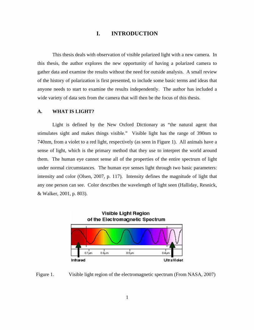
Light is defined by the New Oxford Dictionary as “the natural agent that

stimulates sight and makes things visible.” Visible light has the range of 390nm to

740nm, from a violet to a red light, respectively (as seen in Figure 1). All animals have a

sense of light, which is the primary method that they use to interpret the world around

them. The human eye cannot sense all of the properties of the entire spectrum of light

under normal circumstances. The human eye senses light through two basic parameters:

intensity and color (Olsen, 2007, p. 117). Intensity defines the magnitude of light that

any one person can see. Color describes the wavelength of light seen (Halliday, Resnick,

& Walker, 2001, p. 803).

Figure 1. Visible light region of the electromagnetic spectrum (From NASA, 2007)

2

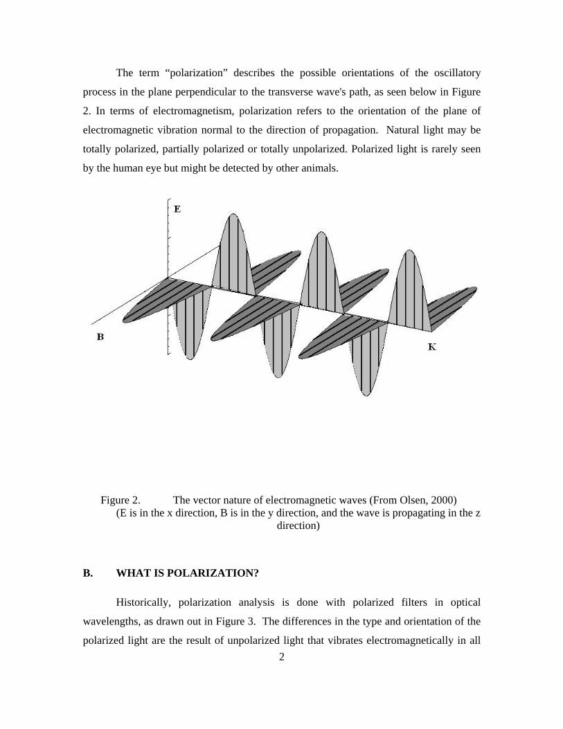
The term “polarization” describes the possible orientations of the oscillatory

process in the plane perpendicular to the transverse wave's path, as seen below in Figure

2. In terms of electromagnetism, polarization refers to the orientation of the plane of

electromagnetic vibration normal to the direction of propagation. Natural light may be

totally polarized, partially polarized or totally unpolarized. Polarized light is rarely seen

by the human eye but might be detected by other animals.

Figure 2. The vector nature of electromagnetic waves (From Olsen, 2000) (E is in the x direction, B is in the y direction, and the wave is propagating in the z

direction)

B. WHAT IS POLARIZATION?

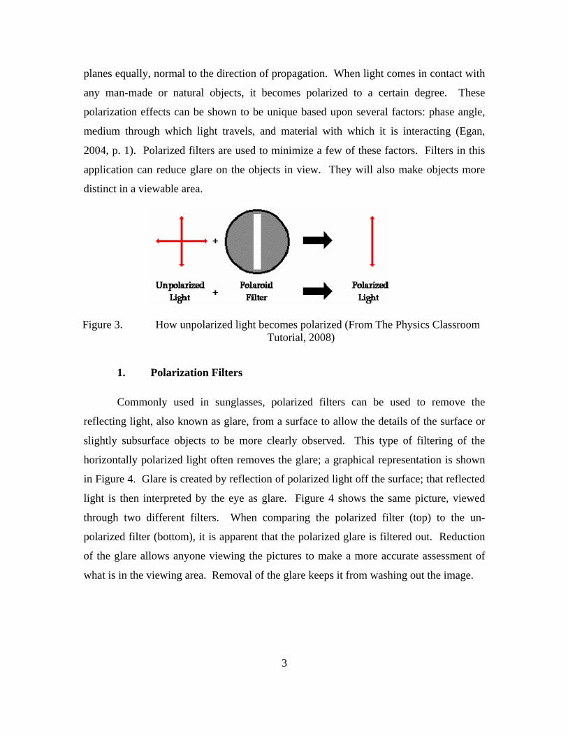
Historically, polarization analysis is done with polarized filters in optical

wavelengths, as drawn out in Figure 3. The differences in the type and orientation of the

polarized light are the result of unpolarized light that vibrates electromagnetically in all

3

planes equally, normal to the direction of propagation. When light comes in contact with

any man-made or natural objects, it becomes polarized to a certain degree. These

polarization effects can be shown to be unique based upon several factors: phase angle,

medium through which light travels, and material with which it is interacting (Egan,

2004, p. 1). Polarized filters are used to minimize a few of these factors. Filters in this

application can reduce glare on the objects in view. They will also make objects more

distinct in a viewable area.

Figure 3. How unpolarized light becomes polarized (From The Physics Classroom Tutorial, 2008)

1. Polarization Filters

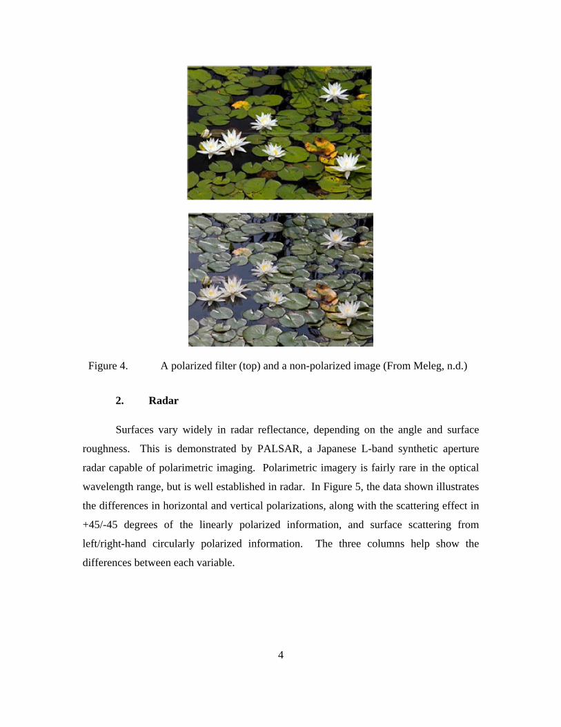
Commonly used in sunglasses, polarized filters can be used to remove the

reflecting light, also known as glare, from a surface to allow the details of the surface or

slightly subsurface objects to be more clearly observed. This type of filtering of the

horizontally polarized light often removes the glare; a graphical representation is shown

in Figure 4. Glare is created by reflection of polarized light off the surface; that reflected

light is then interpreted by the eye as glare. Figure 4 shows the same picture, viewed

through two different filters. When comparing the polarized filter (top) to the un-

polarized filter (bottom), it is apparent that the polarized glare is filtered out. Reduction

of the glare allows anyone viewing the pictures to make a more accurate assessment of

what is in the viewing area. Removal of the glare keeps it from washing out the image.

4

Figure 4. A polarized filter (top) and a non-polarized image (From Meleg, n.d.)

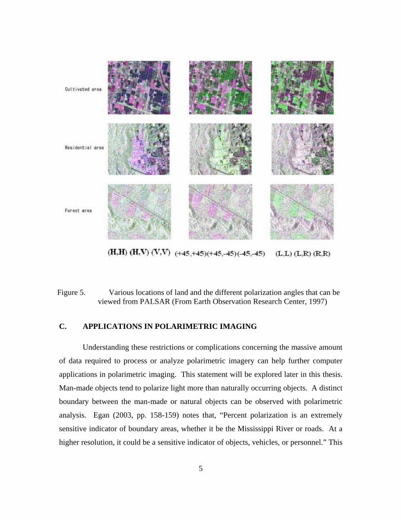
2. Radar

Surfaces vary widely in radar reflectance, depending on the angle and surface

roughness. This is demonstrated by PALSAR, a Japanese L-band synthetic aperture

radar capable of polarimetric imaging. Polarimetric imagery is fairly rare in the optical

wavelength range, but is well established in radar. In Figure 5, the data shown illustrates

the differences in horizontal and vertical polarizations, along with the scattering effect in

+45/-45 degrees of the linearly polarized information, and surface scattering from

left/right-hand circularly polarized information. The three columns help show the

differences between each variable.

5

Figure 5. Various locations of land and the different polarization angles that can be viewed from PALSAR (From Earth Observation Research Center, 1997)

C. APPLICATIONS IN POLARIMETRIC IMAGING

Understanding these restrictions or complications concerning the massive amount

of data required to process or analyze polarimetric imagery can help further computer

applications in polarimetric imaging. This statement will be explored later in this thesis.

Man-made objects tend to polarize light more than naturally occurring objects. A distinct

boundary between the man-made or natural objects can be observed with polarimetric

analysis. Egan (2003, pp. 158-159) notes that, “Percent polarization is an extremely

sensitive indicator of boundary areas, whether it be the Mississippi River or roads. At a

higher resolution, it could be a sensitive indicator of objects, vehicles, or personnel.” This

6

example shows the difference of objects, based on their ability to polarize light. In this

thesis, a new polarizing camera technology is applied to imagery analysis of natural and

man-made scenes.

7

II. HISTORY AND BASICS OF POLARIMETRY

A. POLARIZATION DEFINED

Polarization, sometimes called plane polarization or linear polarization, is an

electromagnetic wave in which the electric vector at a fixed point in space remains

pointing in a fixed direction, although varying in magnitude. A visualization of this can

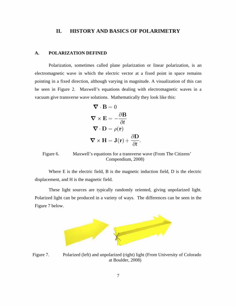
be seen in Figure 2. Maxwell’s equations dealing with electromagnetic waves in a

vacuum give transverse wave solutions. Mathematically they look like this:

Figure 6. Maxwell’s equations for a transverse wave (From The Citizens’ Compendium, 2008)

Where E is the electric field, B is the magnetic induction field, D is the electric

displacement, and H is the magnetic field.

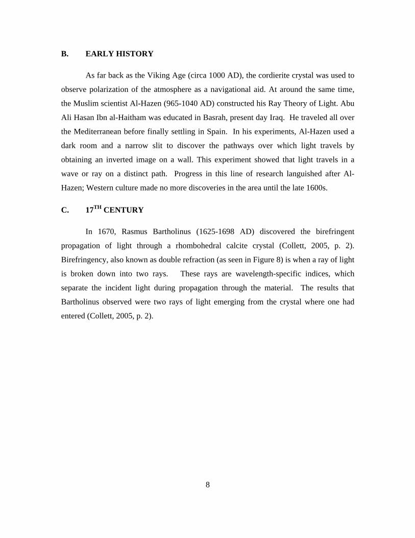
These light sources are typically randomly oriented, giving unpolarized light.

Polarized light can be produced in a variety of ways. The differences can be seen in the

Figure 7 below.

Figure 7. Polarized (left) and unpolarized (right) light (From University of Colorado at Boulder, 2008)

8

B. EARLY HISTORY

As far back as the Viking Age (circa 1000 AD), the cordierite crystal was used to

observe polarization of the atmosphere as a navigational aid. At around the same time,

the Muslim scientist Al-Hazen (965-1040 AD) constructed his Ray Theory of Light. Abu

Ali Hasan Ibn al-Haitham was educated in Basrah, present day Iraq. He traveled all over

the Mediterranean before finally settling in Spain. In his experiments, Al-Hazen used a

dark room and a narrow slit to discover the pathways over which light travels by

obtaining an inverted image on a wall. This experiment showed that light travels in a

wave or ray on a distinct path. Progress in this line of research languished after Al-

Hazen; Western culture made no more discoveries in the area until the late 1600s.

C. 17TH CENTURY

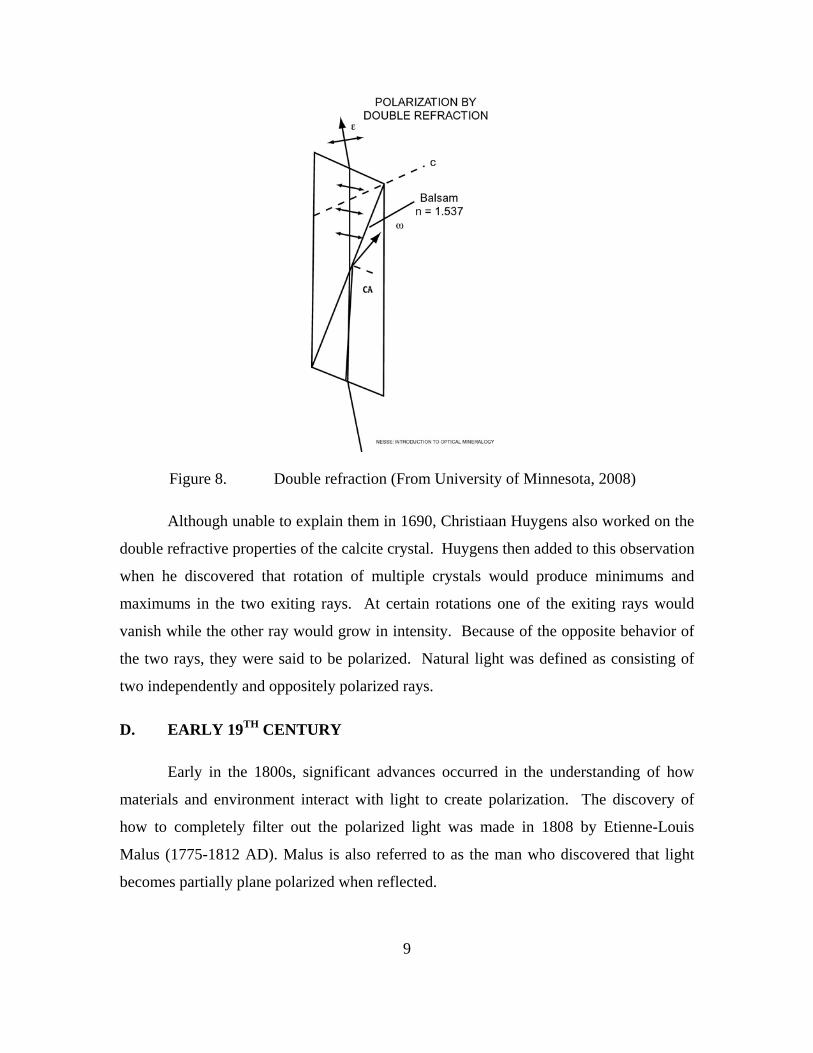
In 1670, Rasmus Bartholinus (1625-1698 AD) discovered the birefringent

propagation of light through a rhombohedral calcite crystal (Collett, 2005, p. 2).

Birefringency, also known as double refraction (as seen in Figure 8) is when a ray of light

is broken down into two rays. These rays are wavelength-specific indices, which

separate the incident light during propagation through the material. The results that

Bartholinus observed were two rays of light emerging from the crystal where one had

entered (Collett, 2005, p. 2).

9

Figure 8. Double refraction (From University of Minnesota, 2008)

Although unable to explain them in 1690, Christiaan Huygens also worked on the

double refractive properties of the calcite crystal. Huygens then added to this observation

when he discovered that rotation of multiple crystals would produce minimums and

maximums in the two exiting rays. At certain rotations one of the exiting rays would

vanish while the other ray would grow in intensity. Because of the opposite behavior of

the two rays, they were said to be polarized. Natural light was defined as consisting of

two independently and oppositely polarized rays.

D. EARLY 19TH CENTURY

Early in the 1800s, significant advances occurred in the understanding of how

materials and environment interact with light to create polarization. The discovery of

how to completely filter out the polarized light was made in 1808 by Etienne-Louis

Malus (1775-1812 AD). Malus is also referred to as the man who discovered that light

becomes partially plane polarized when reflected.

10

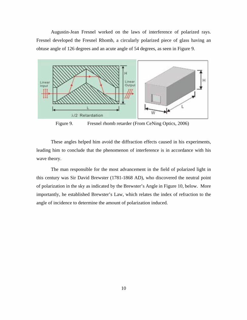
Augustin-Jean Fresnel worked on the laws of interference of polarized rays.

Fresnel developed the Fresnel Rhomb, a circularly polarized piece of glass having an

obtuse angle of 126 degrees and an acute angle of 54 degrees, as seen in Figure 9.

Figure 9. Fresnel rhomb retarder (From CeNing Optics, 2006)

These angles helped him avoid the diffraction effects caused in his experiments,

leading him to conclude that the phenomenon of interference is in accordance with his

wave theory.

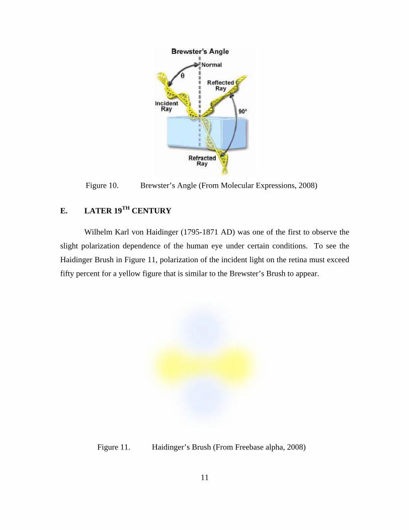
The man responsible for the most advancement in the field of polarized light in

this century was Sir David Brewster (1781-1868 AD), who discovered the neutral point

of polarization in the sky as indicated by the Brewster’s Angle in Figure 10, below. More

importantly, he established Brewster’s Law, which relates the index of refraction to the

angle of incidence to determine the amount of polarization induced.

11

Figure 10. Brewster’s Angle (From Molecular Expressions, 2008)

E. LATER 19TH CENTURY

Wilhelm Karl von Haidinger (1795-1871 AD) was one of the first to observe the

slight polarization dependence of the human eye under certain conditions. To see the

Haidinger Brush in Figure 11, polarization of the incident light on the retina must exceed

fifty percent for a yellow figure that is similar to the Brewster’s Brush to appear.

Figure 11. Haidinger’s Brush (From Freebase alpha, 2008)

12

In 1860, Gustav Kirchhoff (1824-1887) applied his Radiation Law to emanations

from natural substances. He found, in accordance with his law, that incandescent

tourmaline transmits polarized light by a filtration process. Some crystals such as

tourmaline selectively absorb light rays vibrating in one plane, but not those vibrations in

a plane at right angles. Thus, when a beam of light is transmitted through two filters, the

resultant light is polarized in one direction. If one then rotates the second filter by ninety

degrees from the first, no light is transmitted through the filters.

F. 20TH CENTURY

The early 1900s started off with several crucial and important discoveries in the

field of polarimetry. The first among these occurred in 1905, when Umov described how

the albedo and roughness of a surface related to the degree of polarization of the reflected

light (Konnen, 1985, p. 20). The so-called Umov Effect binds color and texture as they

are related to polarization. Umov’s discovery helped show a difference in polarization

between natural objects and man-made objects.

Arguably, the most influential discovery of the twentieth century was made by

Edwin H. Land, who in 1928 constructed the first polarized sheet filter. This innovation

allowed for much simpler and more efficient measurements of light polarization, which

set the foundation for many discoveries in the remainder of the century. Eastman Kodak

bought out Land’s company in 1934 for its light polarizers and photographic filters.

The mid 1900s revealed more about where and how polarized light is found in

nature. Scattered light underwater and starlight are both polarized. Biologically, bees

detect polarized light and use it as the primary method to determine their orientation. In

an experiment, octopus discriminated between light polarized at 45° from light polarized

at 135°, and the experimental situation made it very difficult to explain this by the

perception of scattering or reflexion patterns (Moody, 1962). In 1955, William A.

Shurcliff discovered that humans have the ability to distinguish between unpolarized light

and circularly polarized light. L. F. Jaffe found, in 1956’s “Effect of polarized light in

polarity of Fucus” that when the egg cells of certain algae are exposed to linear light they

develop in the direction of the light vibration.

13

In 1984, the crew of the Space Shuttle took on the roll of image collection for

polarimetric study. The crew of STS51A took a Hasselblad i500 EL/M 70-mm format

camera into space to take polarized images of the Shark Bay atoll. They found that “The

degree of polarization is sensitive to surface roughness. The ocean exhibited lower

radiometric values relative to the barren land but higher polarimetric values under similar

View/illumination geometries” (Israel & Duggin, 1992, p. 3).

Another advance came with the development of POLDER (POLarization and

Directionality of the Earth's Reflectances). POLDER is an imager developed jointly by

the French and Japanese. The first version of this hardware flew in orbit for eight

months, from August 1996 to June 1997. The next evolution flew in space rather

recently, from December 2002 to October 2003. POLDER has provided one of the first

global and systematic measurements of spectral, along with directional and polarized,

characteristics of solar radiation reflected by the Earth’s atmosphere (CNES, 2008).

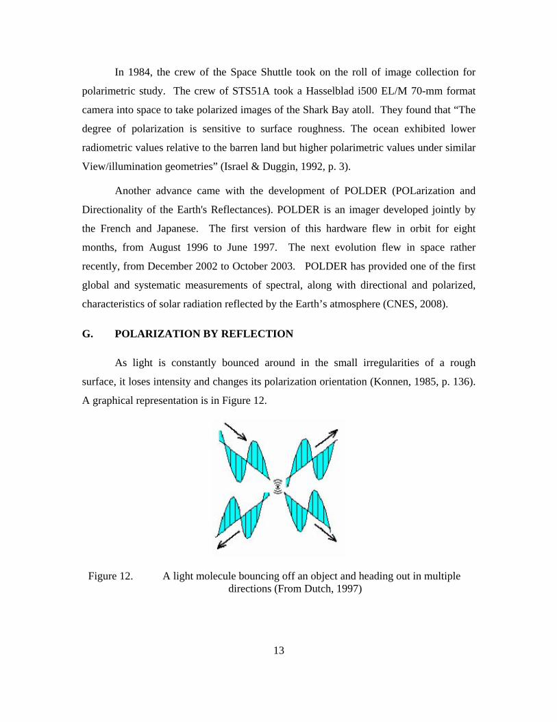
G. POLARIZATION BY REFLECTION

As light is constantly bounced around in the small irregularities of a rough

surface, it loses intensity and changes its polarization orientation (Konnen, 1985, p. 136).

A graphical representation is in Figure 12.

Figure 12. A light molecule bouncing off an object and heading out in multiple directions (From Dutch, 1997)

14

This diminishing effect will reduce the noise that a sensor can detect. A sensor, in

this case a camera, will measure a higher per capita ratio of polarized light in one

direction to the total intensity of the image. The diminishing effect can be detected

because a significant portion of light is weakened, scattered, and/or completely absorbed

at the reflecting surface. The highest degree of polarization is created by a single

reflection. Therefore, a bright, highly reflective surface will contain polarized light

tangential to the plane of the reflection, but it will also contain a significant amount of

light that is not polarized. This will lower the observed percentage of polarization or

degree of polarization (Konnen, 1985, p. 137).

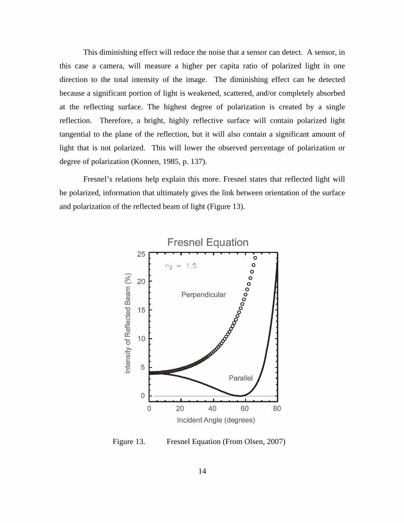
Fresnel’s relations help explain this more. Fresnel states that reflected light will

be polarized, information that ultimately gives the link between orientation of the surface

and polarization of the reflected beam of light (Figure 13).

Figure 13. Fresnel Equation (From Olsen, 2007)

15

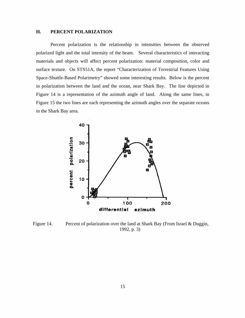
H. PERCENT POLARIZATION

Percent polarization is the relationship in intensities between the observed

polarized light and the total intensity of the beam. Several characteristics of interacting

materials and objects will affect percent polarization: material composition, color and

surface texture. On STS51A, the report “Characterization of Terrestrial Features Using

Space-Shuttle-Based Polarimetry” showed some interesting results. Below is the percent

in polarization between the land and the ocean, near Shark Bay. The line depicted in

Figure 14 is a representation of the azimuth angle of land. Along the same lines, in

Figure 15 the two lines are each representing the azimuth angles over the separate oceans

in the Shark Bay area.

Figure 14. Percent of polarization over the land at Shark Bay (From Israel & Duggin, 1992, p. 3)

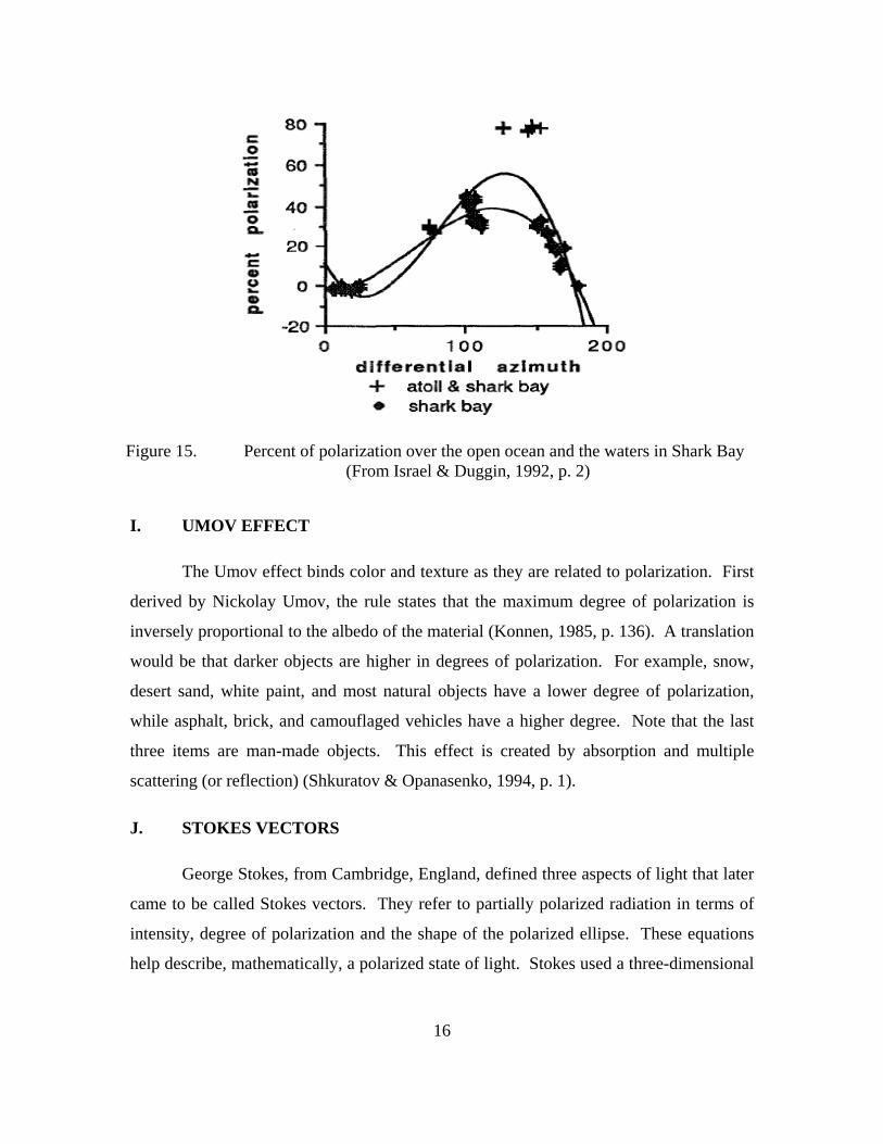
16

Figure 15. Percent of polarization over the open ocean and the waters in Shark Bay (From Israel & Duggin, 1992, p. 2)

I. UMOV EFFECT

The Umov effect binds color and texture as they are related to polarization. First

derived by Nickolay Umov, the rule states that the maximum degree of polarization is

inversely proportional to the albedo of the material (Konnen, 1985, p. 136). A translation

would be that darker objects are higher in degrees of polarization. For example, snow,

desert sand, white paint, and most natural objects have a lower degree of polarization,

while asphalt, brick, and camouflaged vehicles have a higher degree. Note that the last

three items are man-made objects. This effect is created by absorption and multiple

scattering (or reflection) (Shkuratov & Opanasenko, 1994, p. 1).

J. STOKES VECTORS

George Stokes, from Cambridge, England, defined three aspects of light that later

came to be called Stokes vectors. They refer to partially polarized radiation in terms of

intensity, degree of polarization and the shape of the polarized ellipse. These equations

help describe, mathematically, a polarized state of light. Stokes used a three-dimensional

17

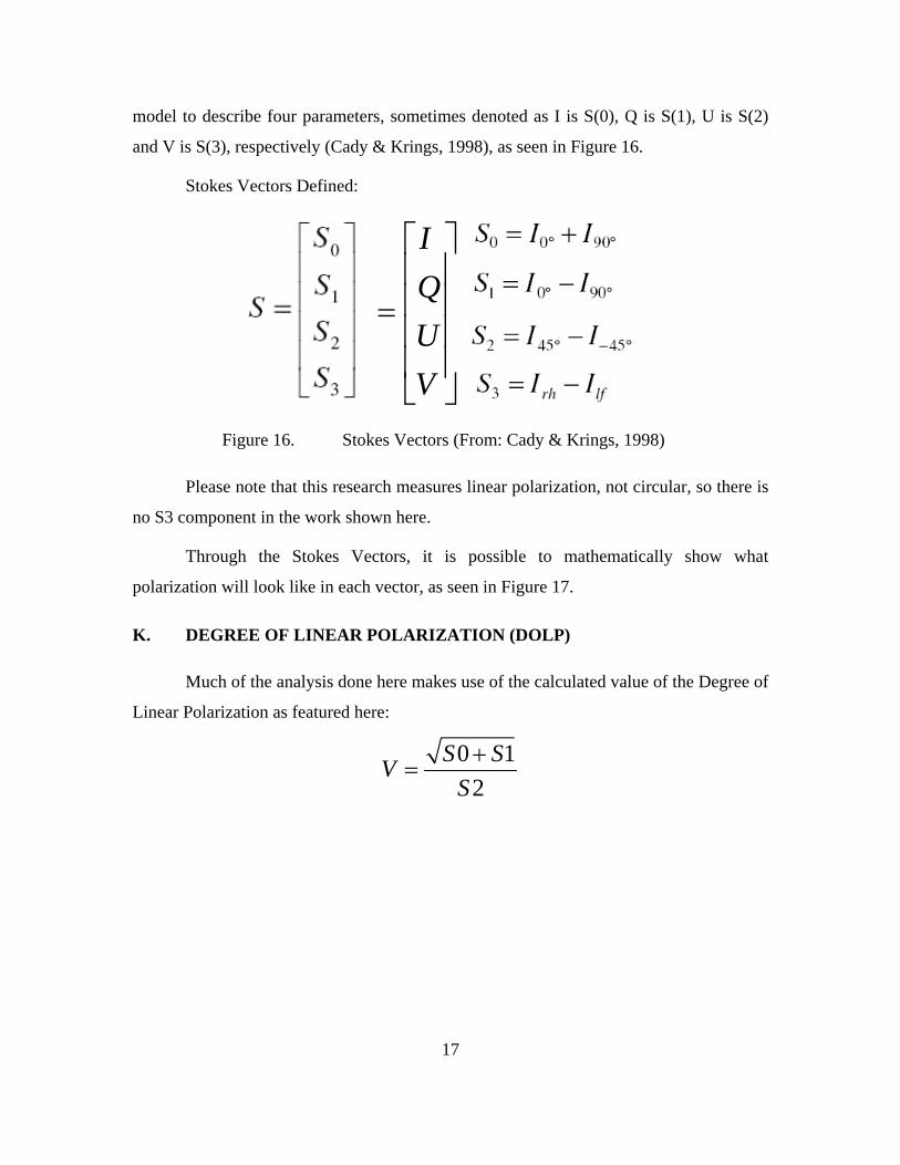
model to describe four parameters, sometimes denoted as I is S(0), Q is S(1), U is S(2)

and V is S(3), respectively (Cady & Krings, 1998), as seen in Figure 16.

Stokes Vectors Defined:

IQUV

⎡ ⎤⎢ ⎥⎢ ⎥=⎢ ⎥⎢ ⎥⎣ ⎦

Figure 16. Stokes Vectors (From: Cady & Krings, 1998)

Please note that this research measures linear polarization, not circular, so there is

no S3 component in the work shown here.

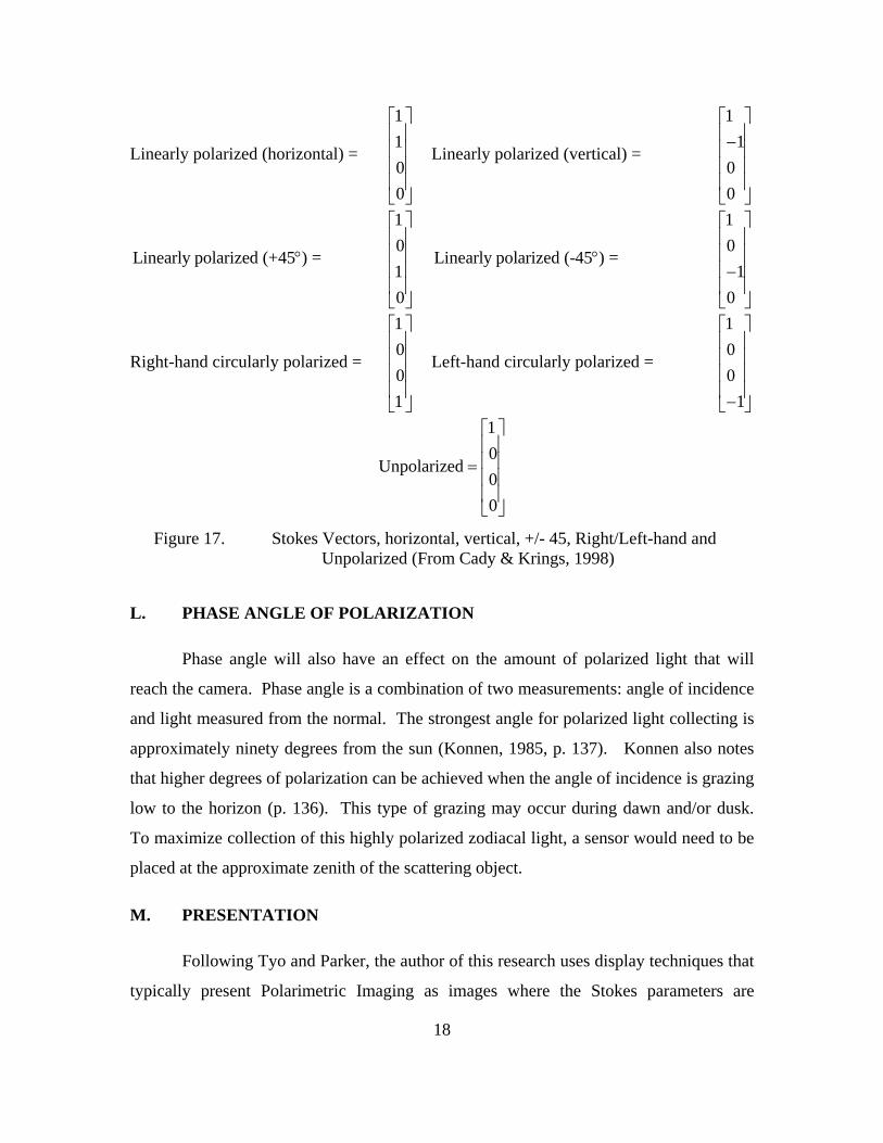
Through the Stokes Vectors, it is possible to mathematically show what

polarization will look like in each vector, as seen in Figure 17.

K. DEGREE OF LINEAR POLARIZATION (DOLP)

Much of the analysis done here makes use of the calculated value of the Degree of

Linear Polarization as featured here:

0 12

S SVS

+=

18

Linearly polarized (horizontal) =

1100

⎡ ⎤⎢ ⎥⎢ ⎥⎢ ⎥⎢ ⎥⎣ ⎦

Linearly polarized (vertical) =

11

00

⎡ ⎤⎢ ⎥−⎢ ⎥⎢ ⎥⎢ ⎥⎣ ⎦

Linearly polarized (+45 ) = °

1010

⎡ ⎤⎢ ⎥⎢ ⎥⎢ ⎥⎢ ⎥⎣ ⎦

Linearly polarized (-45 ) = °

10

10

⎡ ⎤⎢ ⎥⎢ ⎥⎢ ⎥−⎢ ⎥⎣ ⎦

Right-hand circularly polarized =

1001

⎡ ⎤⎢ ⎥⎢ ⎥⎢ ⎥⎢ ⎥⎣ ⎦

Left-hand circularly polarized =

100

1

⎡ ⎤⎢ ⎥⎢ ⎥⎢ ⎥⎢ ⎥−⎣ ⎦

10

Unpolarized00

⎡ ⎤⎢ ⎥⎢ ⎥=⎢ ⎥⎢ ⎥⎣ ⎦

Figure 17. Stokes Vectors, horizontal, vertical, +/- 45, Right/Left-hand and Unpolarized (From Cady & Krings, 1998)

L. PHASE ANGLE OF POLARIZATION

Phase angle will also have an effect on the amount of polarized light that will

reach the camera. Phase angle is a combination of two measurements: angle of incidence

and light measured from the normal. The strongest angle for polarized light collecting is

approximately ninety degrees from the sun (Konnen, 1985, p. 137). Konnen also notes

that higher degrees of polarization can be achieved when the angle of incidence is grazing

low to the horizon (p. 136). This type of grazing may occur during dawn and/or dusk.

To maximize collection of this highly polarized zodiacal light, a sensor would need to be

placed at the approximate zenith of the scattering object.

M. PRESENTATION

Following Tyo and Parker, the author of this research uses display techniques that

typically present Polarimetric Imaging as images where the Stokes parameters are

19

encoded in gray scale or color, with intensity, DOLP, or polarized angles as the primary

element of interest. An approach typically used here is to encode the average intensity

(S0) as intensity, the angle of polarization (S1) as hue, and DOLP as saturation (S2) in a

hue-saturation intensity (also known as Hue Sat value) color scheme (Tyo, et al., 2006;

Parker, 2007). More commonly, following Parker, the S0 is encoded as intensity, the

DOLP as hue and the S2 as saturation to obtain a more invariant display approach. This

seems to provide measurement parameters that are not as sensitive to external factors,

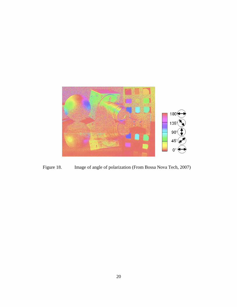
such as illumination and view angles. Figure 18 shows an image of what phase angle of

polarization can give you visually.

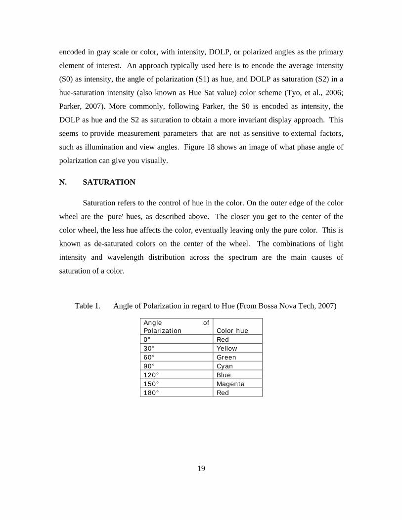
N. SATURATION

Saturation refers to the control of hue in the color. On the outer edge of the color

wheel are the 'pure' hues, as described above. The closer you get to the center of the

color wheel, the less hue affects the color, eventually leaving only the pure color. This is

known as de-saturated colors on the center of the wheel. The combinations of light

intensity and wavelength distribution across the spectrum are the main causes of

saturation of a color.

Table 1. Angle of Polarization in regard to Hue (From Bossa Nova Tech, 2007)

Angle of Polarization Color hue 0° Red 30° Yellow 60° Green 90° Cyan 120° Blue 150° Magenta 180° Red

20

Figure 18. Image of angle of polarization (From Bossa Nova Tech, 2007)

21

III. CAMERA OPERATIONS

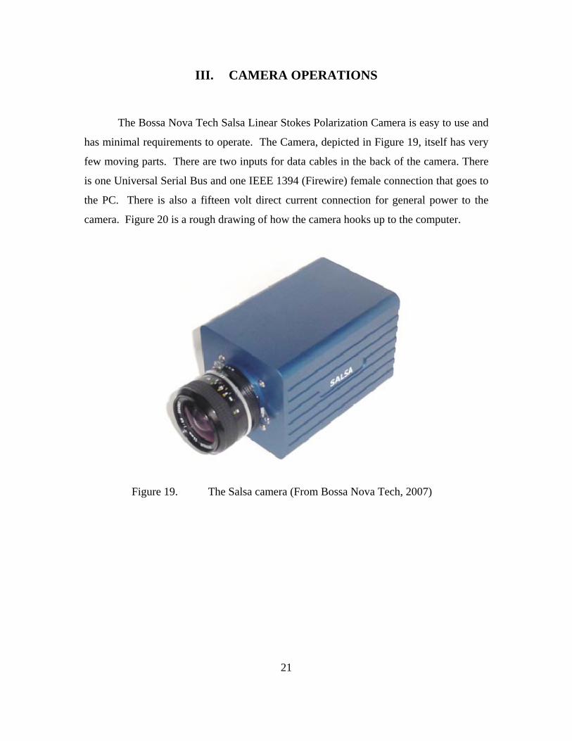
The Bossa Nova Tech Salsa Linear Stokes Polarization Camera is easy to use and

has minimal requirements to operate. The Camera, depicted in Figure 19, itself has very

few moving parts. There are two inputs for data cables in the back of the camera. There

is one Universal Serial Bus and one IEEE 1394 (Firewire) female connection that goes to

the PC. There is also a fifteen volt direct current connection for general power to the

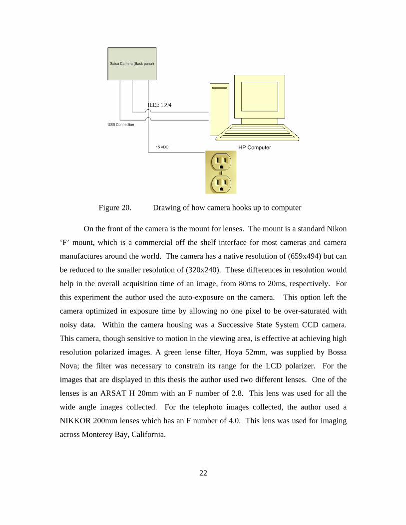
camera. Figure 20 is a rough drawing of how the camera hooks up to the computer.

Figure 19. The Salsa camera (From Bossa Nova Tech, 2007)

22

Figure 20. Drawing of how camera hooks up to computer

On the front of the camera is the mount for lenses. The mount is a standard Nikon

‘F’ mount, which is a commercial off the shelf interface for most cameras and camera

manufactures around the world. The camera has a native resolution of (659x494) but can

be reduced to the smaller resolution of (320x240). These differences in resolution would

help in the overall acquisition time of an image, from 80ms to 20ms, respectively. For

this experiment the author used the auto-exposure on the camera. This option left the

camera optimized in exposure time by allowing no one pixel to be over-saturated with

noisy data. Within the camera housing was a Successive State System CCD camera.

This camera, though sensitive to motion in the viewing area, is effective at achieving high

resolution polarized images. A green lense filter, Hoya 52mm, was supplied by Bossa

Nova; the filter was necessary to constrain its range for the LCD polarizer. For the

images that are displayed in this thesis the author used two different lenses. One of the

lenses is an ARSAT H 20mm with an F number of 2.8. This lens was used for all the

wide angle images collected. For the telephoto images collected, the author used a

NIKKOR 200mm lenses which has an F number of 4.0. This lens was used for imaging

across Monterey Bay, California.

23

For this experiment, the author used a Hewlett-Packard Pavilion Slimline s3400z,

which has a dual core Advance Micro Devices processor (BE-2400) running at 2.30 GHz.

The system came equipped with 4 GB of memory, and the 32 bit version of Windows

Vista Home Premium with service pack 1 installed. To run the Bossa Nova Tech Salsa

Linear Stokes Polarization Imaging Software—a requirement for taking pictures—the

software key (an actual, physical device) needs to be inserted into one of the Universal

Serial Bus (USB) ports on the computer. In addition to the key, the cables need to be

plugged into the appropriate ports on the computer. The camera requires at least one

USB port and one Firewire port on the computer. The final requirement is power; the

camera runs off a power adaptor that gives a 15 volt/1.2 amp output.

The software Bossa Nova has developed is rather simple to use and easily

navigable. Throughout this thesis, the author enjoyed a great dialog with the developers

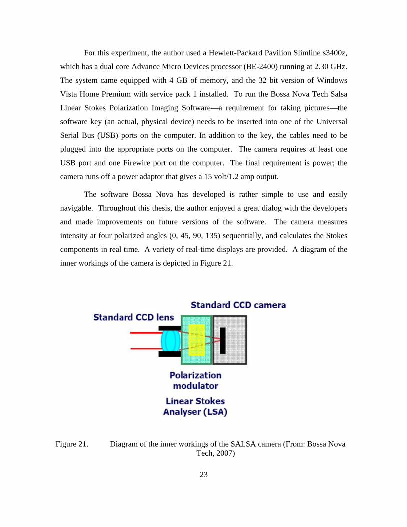
and made improvements on future versions of the software. The camera measures

intensity at four polarized angles (0, 45, 90, 135) sequentially, and calculates the Stokes

components in real time. A variety of real-time displays are provided. A diagram of the

inner workings of the camera is depicted in Figure 21.

Figure 21. Diagram of the inner workings of the SALSA camera (From: Bossa Nova Tech, 2007)

24

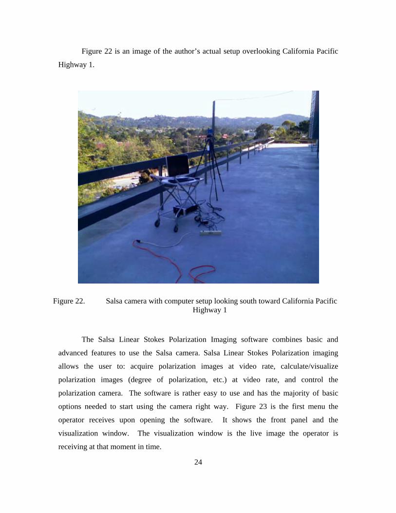
Figure 22 is an image of the author’s actual setup overlooking California Pacific

Highway 1.

Figure 22. Salsa camera with computer setup looking south toward California Pacific Highway 1

The Salsa Linear Stokes Polarization Imaging software combines basic and

advanced features to use the Salsa camera. Salsa Linear Stokes Polarization imaging

allows the user to: acquire polarization images at video rate, calculate/visualize

polarization images (degree of polarization, etc.) at video rate, and control the

polarization camera. The software is rather easy to use and has the majority of basic

options needed to start using the camera right way. Figure 23 is the first menu the

operator receives upon opening the software. It shows the front panel and the

visualization window. The visualization window is the live image the operator is

receiving at that moment in time.

25

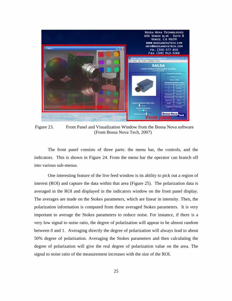
Figure 23. Front Panel and Visualization Window from the Bossa Nova software (From Bossa Nova Tech, 2007)

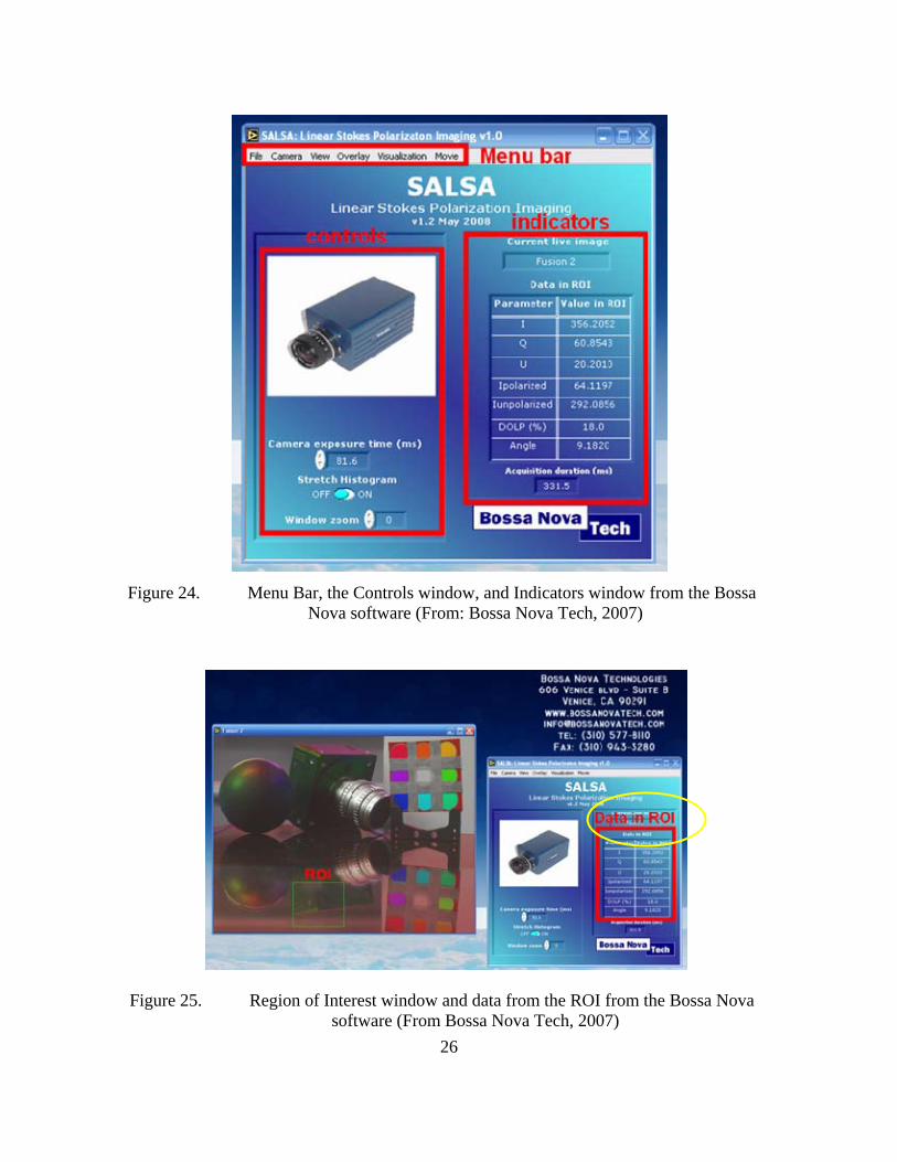
The front panel consists of three parts: the menu bar, the controls, and the

indicators. This is shown in Figure 24. From the menu bar the operator can branch off

into various sub-menus.

One interesting feature of the live feed window is its ability to pick out a region of

interest (ROI) and capture the data within that area (Figure 25). The polarization data is

averaged in the ROI and displayed in the indicators window on the front panel display.

The averages are made on the Stokes parameters, which are linear in intensity. Then, the

polarization information is computed from these averaged Stokes parameters. It is very

important to average the Stokes parameters to reduce noise. For instance, if there is a

very low signal to noise ratio, the degree of polarization will appear to be almost random

between 0 and 1. Averaging directly the degree of polarization will always lead to about

50% degree of polarization. Averaging the Stokes parameters and then calculating the

degree of polarization will give the real degree of polarization value on the area. The

signal to noise ratio of the measurement increases with the size of the ROI.

26

Figure 24. Menu Bar, the Controls window, and Indicators window from the Bossa Nova software (From: Bossa Nova Tech, 2007)

Figure 25. Region of Interest window and data from the ROI from the Bossa Nova software (From Bossa Nova Tech, 2007)

27

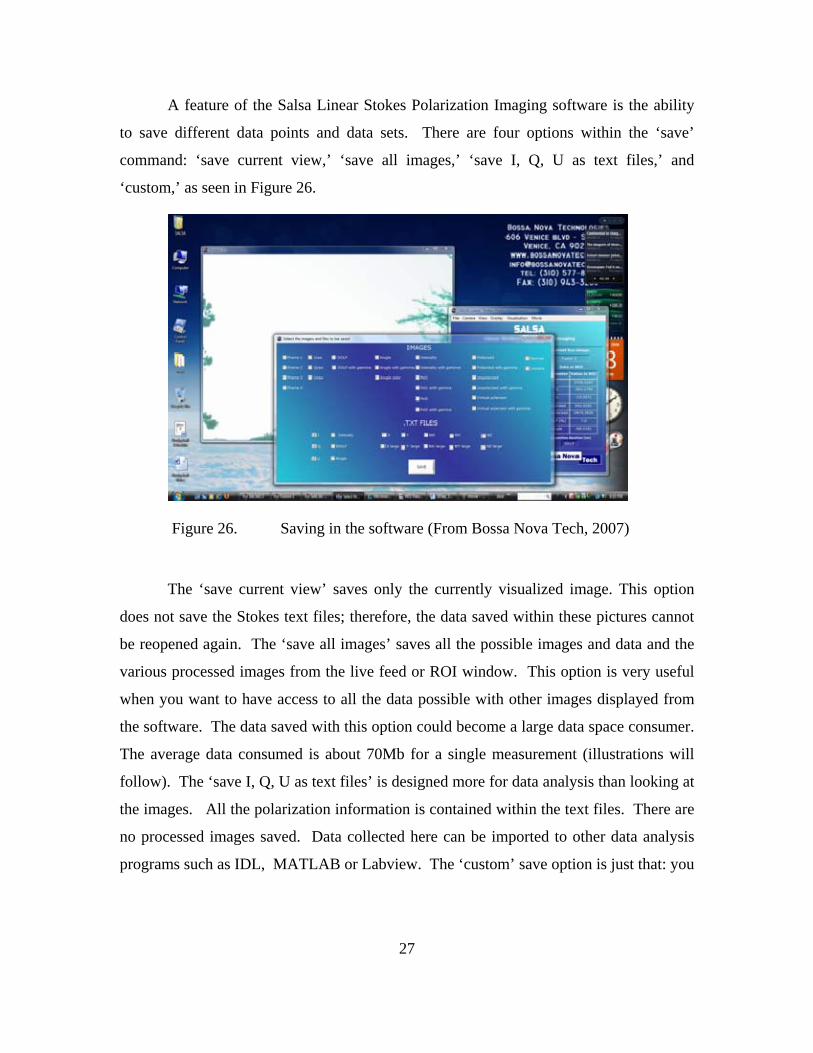
A feature of the Salsa Linear Stokes Polarization Imaging software is the ability

to save different data points and data sets. There are four options within the ‘save’

command: ‘save current view,’ ‘save all images,’ ‘save I, Q, U as text files,’ and

‘custom,’ as seen in Figure 26.

Figure 26. Saving in the software (From Bossa Nova Tech, 2007)

The ‘save current view’ saves only the currently visualized image. This option

does not save the Stokes text files; therefore, the data saved within these pictures cannot

be reopened again. The ‘save all images’ saves all the possible images and data and the

various processed images from the live feed or ROI window. This option is very useful

when you want to have access to all the data possible with other images displayed from

the software. The data saved with this option could become a large data space consumer.

The average data consumed is about 70Mb for a single measurement (illustrations will

follow). The ‘save I, Q, U as text files’ is designed more for data analysis than looking at

the images. All the polarization information is contained within the text files. There are

no processed images saved. Data collected here can be imported to other data analysis

programs such as IDL, MATLAB or Labview. The ‘custom’ save option is just that: you

28

can do any of the previous options plus a lot more. For example, if you want intensity,

degree of polarization and angle of polarization but do not want the unpolarized images,

this is the option you can use.

Like any other camera, the Salsa camera is equipped with a few basic functions:

Auto exposure, Gain and Resolution. With ‘autoexposure’ you can optimize the

exposure time to avoid overexposing some parts of the image. The best exposure time is

the one that will not overexpose the part of the image you are interested in. This option

gives you the advantage of not over-saturating any one pixel, which can lead to dark

images along with noisy data if there are bright reflections in the image. If the part of the

image you are interested in is dark, you can manually adjust the exposure time to reduce

noise. The Gain function allows you to choose from among three preset camera gains.

The lowest gain is associated with the lowest noise on the data and images. Gain can be

increased if the picture is very dark. It can also be amplified if you want to decrease the

acquisition duration by reducing the exposure time. The Resolution option allows

changing the resolution of the camera from the native (659x494) resolution to a smaller

(320x240) resolution. The lower resolution reduces the acquisition and processing times

and speeds display. In low resolution, the maximum exposure time is 20ms, whereas it is

80ms for the highest resolution. Something to keep in mind is that there is no

improvement in speed with a reduced resolution if the exposure time is above 20ms.

Reduce the resolution of the camera if you want to reduce the acquisition time to avoid

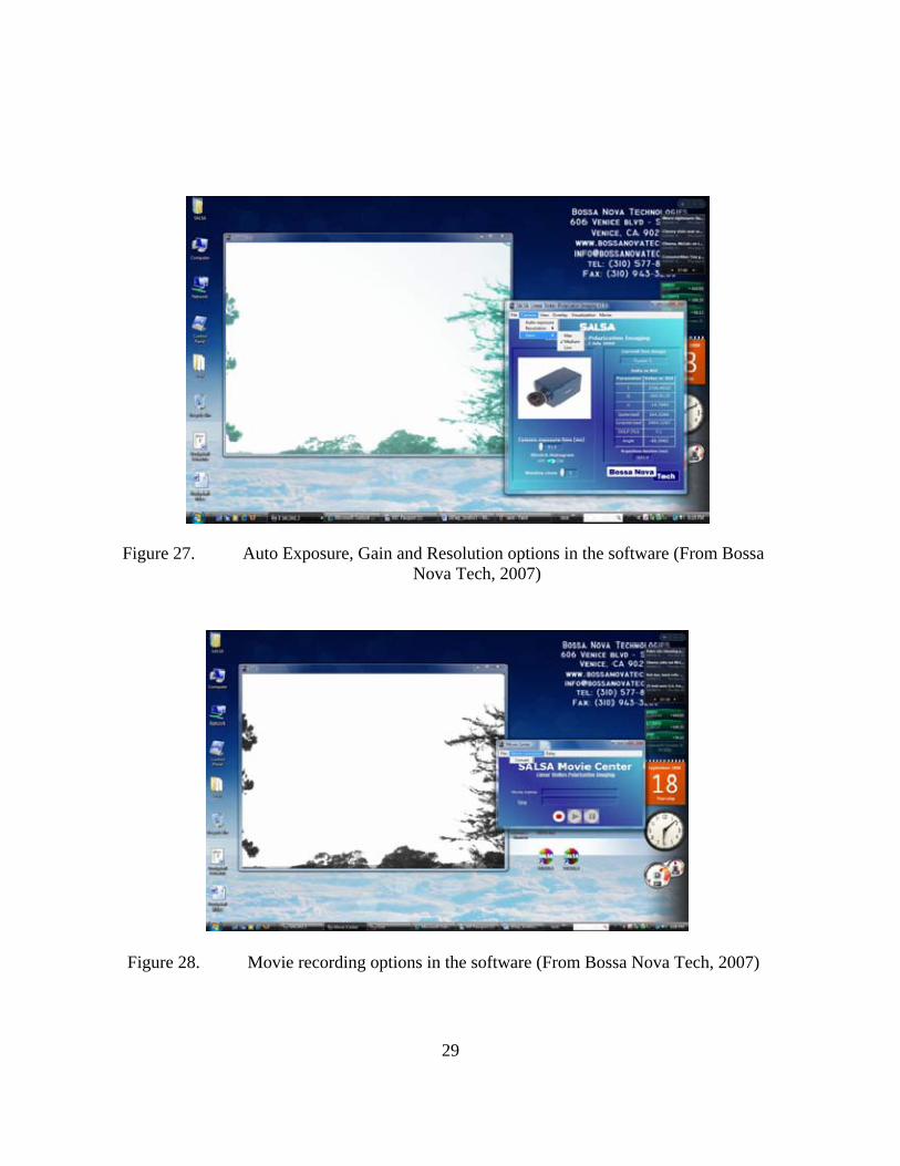
motion effects. These options are shown in Figure 27.

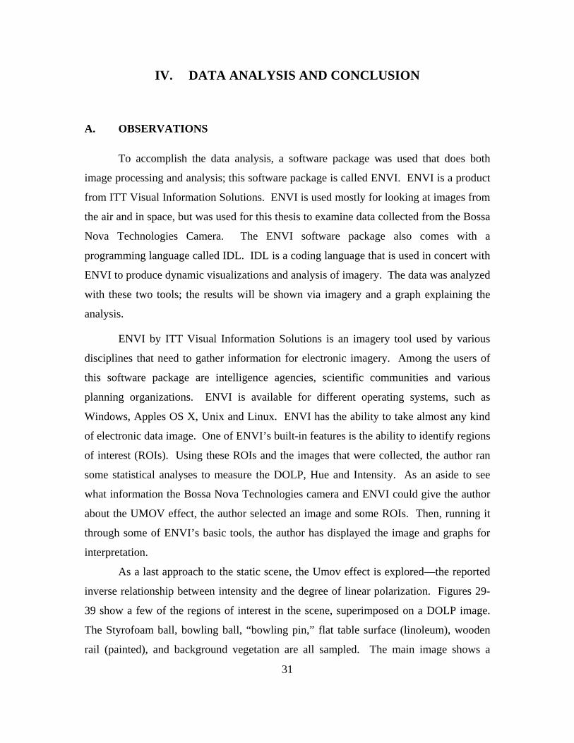
The camera also has a developing tool that Bossa Nova is experimenting with,

which uses the camera in a movie making sense. Within the software there is a sub-

heading for ‘Movie.’ This opens the movie center, shown in Figure 28. From here, you

can record as with a normal video camera. One of the initial troubles with this recording

option was that it only recorded data in AVI format—not the best format from which to

attempt to extract further information. The vendor is developing alternate video storage

formats that will allow for further processing the data.

29

Figure 27. Auto Exposure, Gain and Resolution options in the software (From Bossa Nova Tech, 2007)

Figure 28. Movie recording options in the software (From Bossa Nova Tech, 2007)

30


31

IV. DATA ANALYSIS AND CONCLUSION

A. OBSERVATIONS

To accomplish the data analysis, a software package was used that does both

image processing and analysis; this software package is called ENVI. ENVI is a product

from ITT Visual Information Solutions. ENVI is used mostly for looking at images from

the air and in space, but was used for this thesis to examine data collected from the Bossa

Nova Technologies Camera. The ENVI software package also comes with a

programming language called IDL. IDL is a coding language that is used in concert with

ENVI to produce dynamic visualizations and analysis of imagery. The data was analyzed

with these two tools; the results will be shown via imagery and a graph explaining the

analysis.

ENVI by ITT Visual Information Solutions is an imagery tool used by various

disciplines that need to gather information for electronic imagery. Among the users of

this software package are intelligence agencies, scientific communities and various

planning organizations. ENVI is available for different operating systems, such as

Windows, Apples OS X, Unix and Linux. ENVI has the ability to take almost any kind

of electronic data image. One of ENVI’s built-in features is the ability to identify regions

of interest (ROIs). Using these ROIs and the images that were collected, the author ran

some statistical analyses to measure the DOLP, Hue and Intensity. As an aside to see

what information the Bossa Nova Technologies camera and ENVI could give the author

about the UMOV effect, the author selected an image and some ROIs. Then, running it

through some of ENVI’s basic tools, the author has displayed the image and graphs for

interpretation.

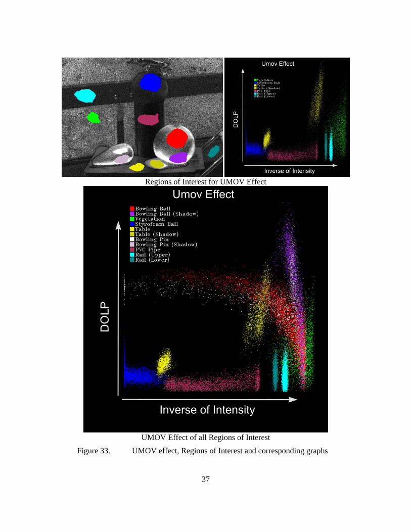
As a last approach to the static scene, the Umov effect is explored—the reported

inverse relationship between intensity and the degree of linear polarization. Figures 29-

39 show a few of the regions of interest in the scene, superimposed on a DOLP image.

The Styrofoam ball, bowling ball, “bowling pin,” flat table surface (linoleum), wooden

rail (painted), and background vegetation are all sampled. The main image shows a

32

scatter plot of the two parameters, the smaller inset plot removes the hard surfaces of the

bowling ball and pin, to make the vegetation clearer. There is some correlation between

the two imaging dimensions, but also some differentiation. DOLP is sensitive to shade,

particularly since the reflection in the shaded region includes elements from other nearby

surfaces. The Styrofoam ball, table, and PVC pipe show differentiation in brightness,

but the table in particular is distinguished from those two surfaces by polarization.

There were two avenues of approach to looking at the images. The first was to

look at the images that were single shot images (Figures 29 through 39), like still photos

or paintings.

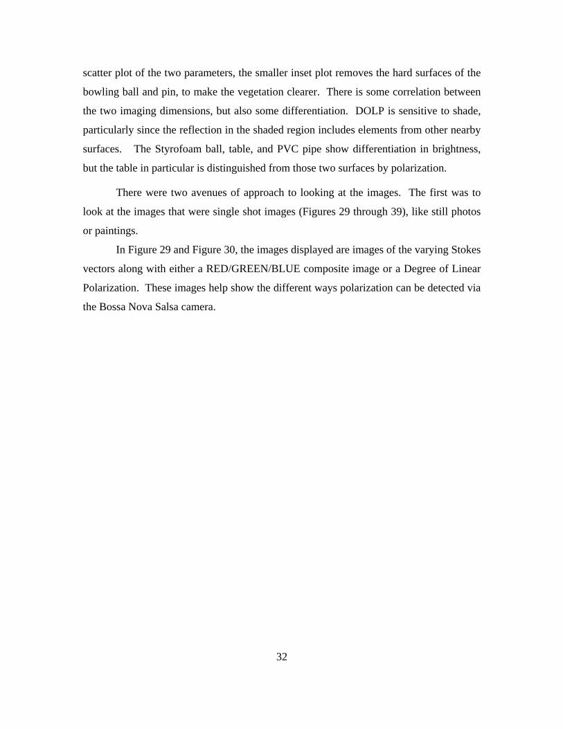
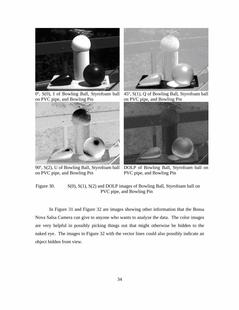
In Figure 29 and Figure 30, the images displayed are images of the varying Stokes

vectors along with either a RED/GREEN/BLUE composite image or a Degree of Linear

Polarization. These images help show the different ways polarization can be detected via

the Bossa Nova Salsa camera.

33

Raw Measurements at 0º, 45º, and 90º, 135 º in an RGB composite

0º, S(0), I of Bowling Ball, Styrofoam ball on PVC pipe, and Bowling Pin

45º, S(1), Q of Bowling Ball, Styrofoam ball on PVC pipe, and Bowling Pin

90º, S(2), U of Bowling Ball, Styrofoam ball on PVC pipe, and Bowling Pin

135º, S(3), V of Bowling Ball, Styrofoam ball on PVC pipe, and Bowling Pin

Figure 29. Images S(0), S(1), S(2), & S(3) along with RGB composite

34

0º, S(0), I of Bowling Ball, Styrofoam ball on PVC pipe, and Bowling Pin

45º, S(1), Q of Bowling Ball, Styrofoam ball on PVC pipe, and Bowling Pin

90º, S(2), U of Bowling Ball, Styrofoam ball on PVC pipe, and Bowling Pin

DOLP of Bowling Ball, Styrofoam ball on PVC pipe, and Bowling Pin

Figure 30. S(0), S(1), S(2) and DOLP images of Bowling Ball, Styrofoam ball on PVC pipe, and Bowling Pin

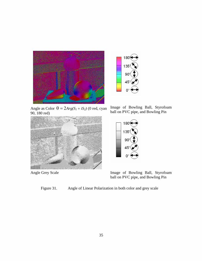
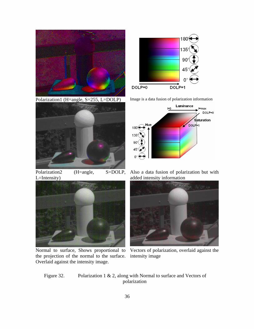
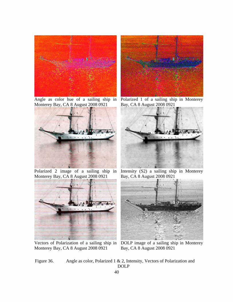
In Figure 31 and Figure 32 are images showing other information that the Bossa

Nova Salsa Camera can give to anyone who wants to analyze the data. The color images

are very helpful in possibly picking things out that might otherwise be hidden to the

naked eye. The images in Figure 32 with the vector lines could also possibly indicate an

object hidden from view.

35

Angle as Color θ = 2Arg(S1 + iS2) (0 red, cyan 90, 180 red)

Image of Bowling Ball, Styrofoam ball on PVC pipe, and Bowling Pin

Angle Grey Scale Image of Bowling Ball, Styrofoam ball on PVC pipe, and Bowling Pin

Figure 31. Angle of Linear Polarization in both color and grey scale

36

Polarization1 (H=angle, S=255, L=DOLP) Image is a data fusion of polarization information

Polarization2 (H=angle, S=DOLP, L=Intensity)

Also a data fusion of polarization but with added intensity information

Normal to surface, Shows proportional to the projection of the normal to the surface. Overlaid against the intensity image.

Vectors of polarization, overlaid against the intensity image

Figure 32. Polarization 1 & 2, along with Normal to surface and Vectors of polarization

37

Regions of Interest for UMOV Effect

UMOV Effect of all Regions of Interest

Figure 33. UMOV effect, Regions of Interest and corresponding graphs

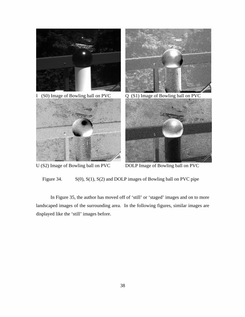
38

I (S0) Image of Bowling ball on PVC Q (S1) Image of Bowling ball on PVC

U (S2) Image of Bowling ball on PVC DOLP Image of Bowling ball on PVC

Figure 34. S(0), S(1), S(2) and DOLP images of Bowling ball on PVC pipe

In Figure 35, the author has moved off of ‘still’ or ‘staged’ images and on to more

landscaped images of the surrounding area. In the following figures, similar images are

displayed like the ‘still’ images before.

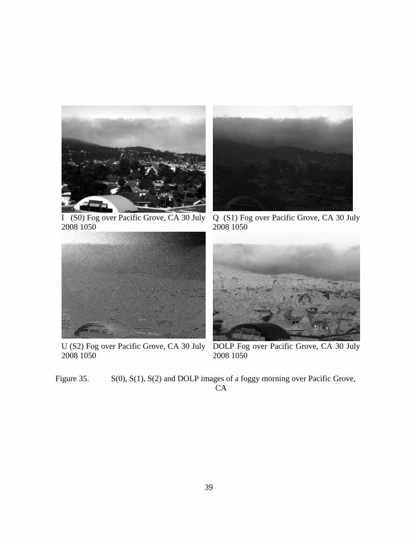
39

I (S0) Fog over Pacific Grove, CA 30 July 2008 1050

Q (S1) Fog over Pacific Grove, CA 30 July 2008 1050

U (S2) Fog over Pacific Grove, CA 30 July 2008 1050

DOLP Fog over Pacific Grove, CA 30 July 2008 1050

Figure 35. S(0), S(1), S(2) and DOLP images of a foggy morning over Pacific Grove, CA

40

Angle as color hue of a sailing ship in Monterey Bay, CA 8 August 2008 0921

Polarized 1 of a sailing ship in Monterey Bay, CA 8 August 2008 0921

Polarized 2 image of a sailing ship in Monterey Bay, CA 8 August 2008 0921

Intensity (S2) a sailing ship in Monterey Bay, CA 8 August 2008 0921

Vectors of Polarization of a sailing ship in Monterey Bay, CA 8 August 2008 0921

DOLP image of a sailing ship in Monterey Bay, CA 8 August 2008 0921

Figure 36. Angle as color, Polarized 1 & 2, Intensity, Vectors of Polarization and DOLP

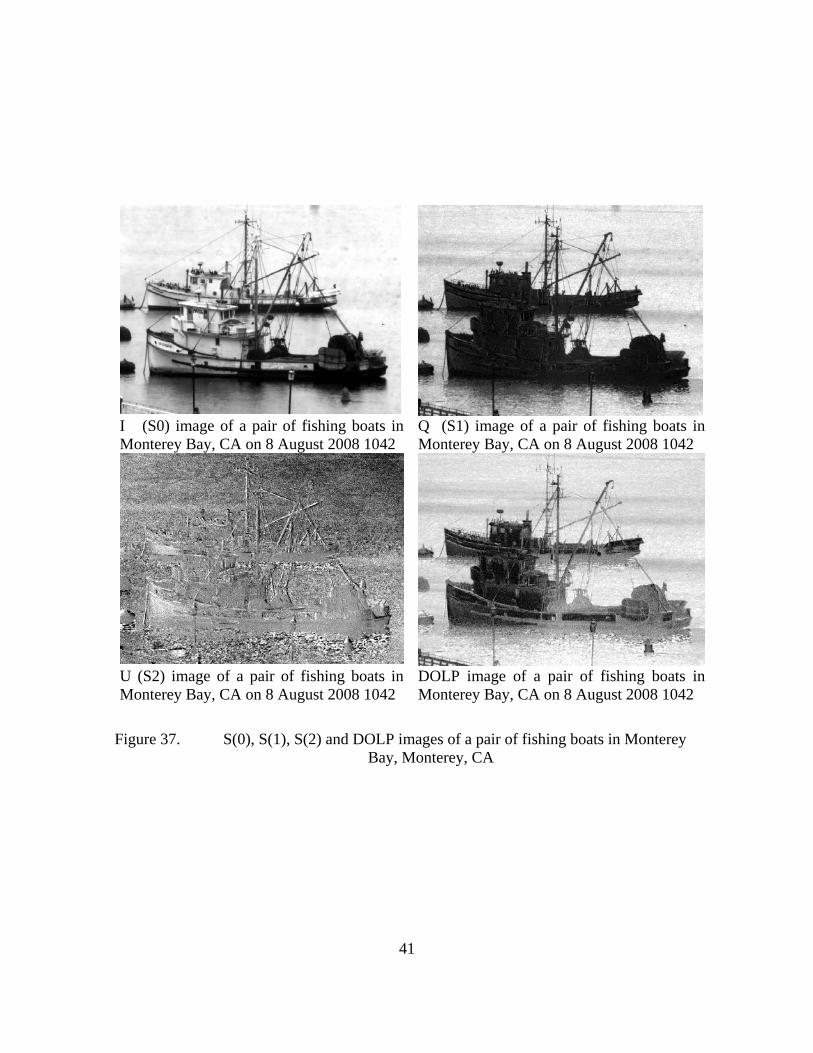
41

I (S0) image of a pair of fishing boats in Monterey Bay, CA on 8 August 2008 1042

Q (S1) image of a pair of fishing boats in Monterey Bay, CA on 8 August 2008 1042

U (S2) image of a pair of fishing boats in Monterey Bay, CA on 8 August 2008 1042

DOLP image of a pair of fishing boats in Monterey Bay, CA on 8 August 2008 1042

Figure 37. S(0), S(1), S(2) and DOLP images of a pair of fishing boats in Monterey Bay, Monterey, CA

42

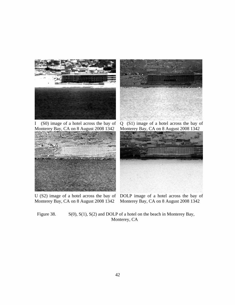
I (S0) image of a hotel across the bay of Monterey Bay, CA on 8 August 2008 1342

Q (S1) image of a hotel across the bay of Monterey Bay, CA on 8 August 2008 1342

U (S2) image of a hotel across the bay of Monterey Bay, CA on 8 August 2008 1342

DOLP image of a hotel across the bay of Monterey Bay, CA on 8 August 2008 1342

Figure 38. S(0), S(1), S(2) and DOLP of a hotel on the beach in Monterey Bay, Monterey, CA

43

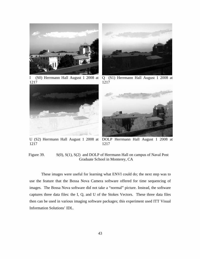
I (S0) Herrmann Hall August 1 2008 at 1217

Q (S1) Herrmann Hall August 1 2008 at 1217

U (S2) Herrmann Hall August 1 2008 at 1217

DOLP Herrmann Hall August 1 2008 at 1217

Figure 39. S(0), S(1), S(2) and DOLP of Herrmann Hall on campus of Naval Post Graduate School in Monterey, CA

These images were useful for learning what ENVI could do; the next step was to

use the feature that the Bossa Nova Camera software offered for time sequencing of

images. The Bossa Nova software did not take a “normal” picture. Instead, the software

captures three data files: the I, Q, and U of the Stokes Vectors. These three data files

then can be used in various imaging software packages; this experiment used ITT Visual

Information Solutions’ IDL.

44

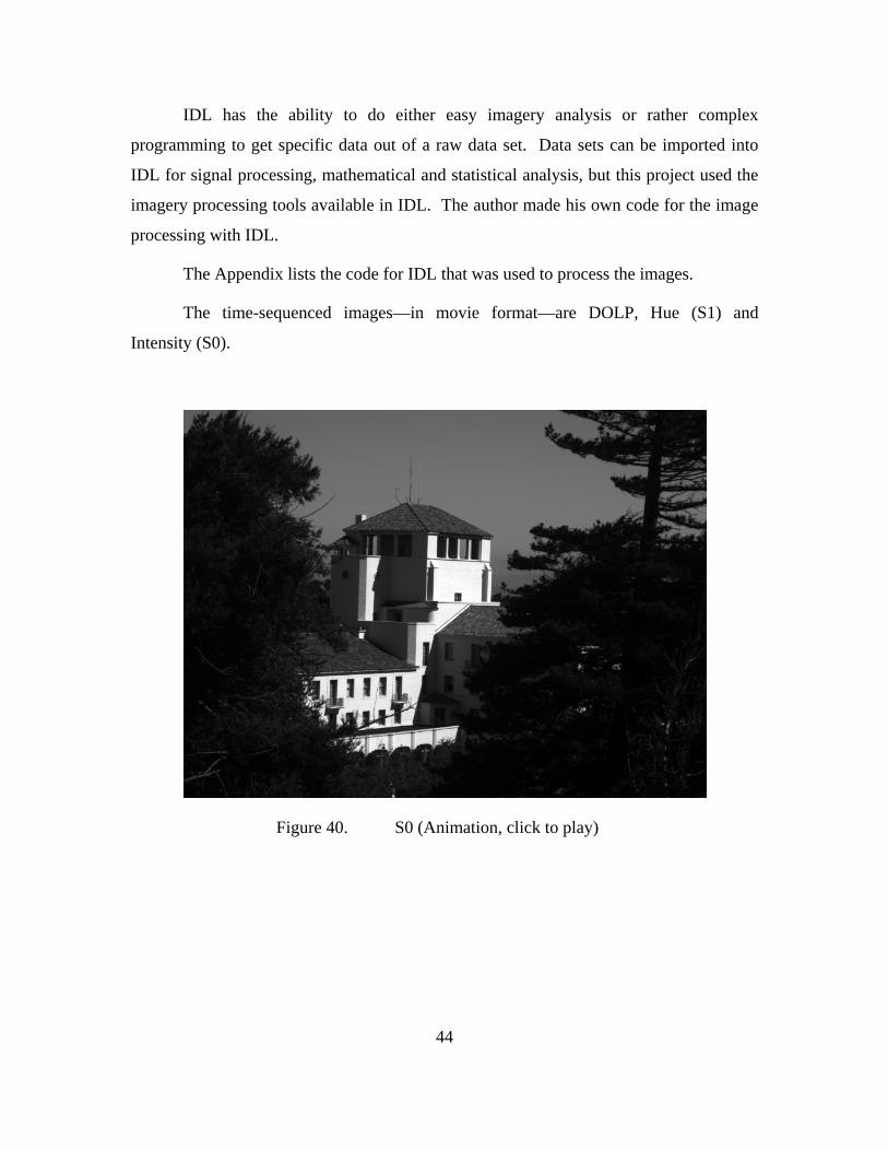
IDL has the ability to do either easy imagery analysis or rather complex

programming to get specific data out of a raw data set. Data sets can be imported into

IDL for signal processing, mathematical and statistical analysis, but this project used the

imagery processing tools available in IDL. The author made his own code for the image

processing with IDL.

The Appendix lists the code for IDL that was used to process the images.

The time-sequenced images—in movie format—are DOLP, Hue (S1) and

Intensity (S0).

Figure 40. S0 (Animation, click to play)

45

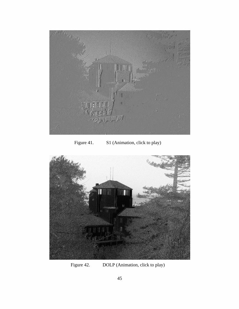
Figure 41. S1 (Animation, click to play)

Figure 42. DOLP (Animation, click to play)

46

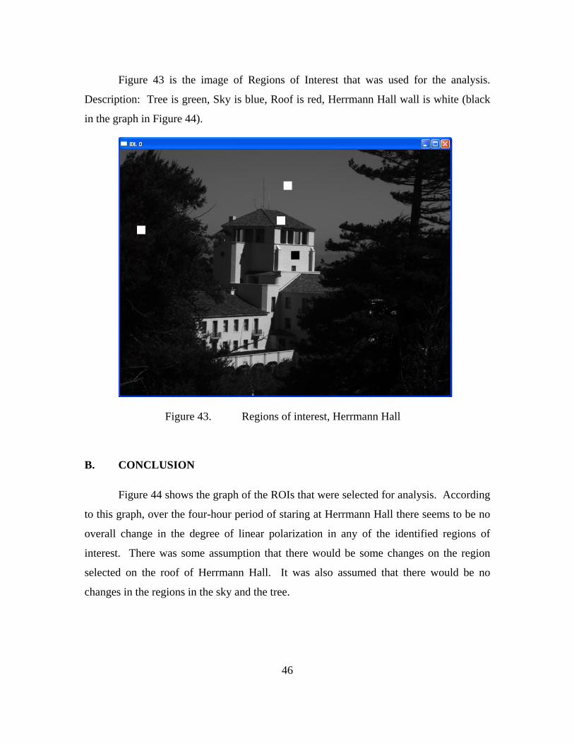
Figure 43 is the image of Regions of Interest that was used for the analysis.

Description: Tree is green, Sky is blue, Roof is red, Herrmann Hall wall is white (black

in the graph in Figure 44).

Figure 43. Regions of interest, Herrmann Hall

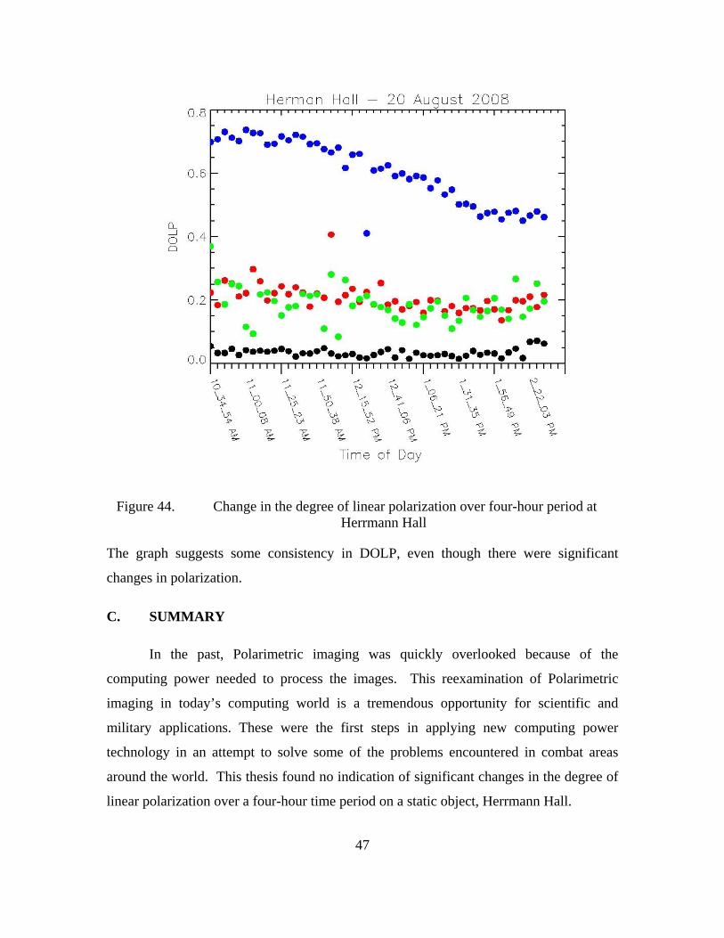
B. CONCLUSION

Figure 44 shows the graph of the ROIs that were selected for analysis. According

to this graph, over the four-hour period of staring at Herrmann Hall there seems to be no

overall change in the degree of linear polarization in any of the identified regions of

interest. There was some assumption that there would be some changes on the region

selected on the roof of Herrmann Hall. It was also assumed that there would be no

changes in the regions in the sky and the tree.

47

Figure 44. Change in the degree of linear polarization over four-hour period at

Herrmann Hall

The graph suggests some consistency in DOLP, even though there were significant

changes in polarization.

C. SUMMARY

In the past, Polarimetric imaging was quickly overlooked because of the

computing power needed to process the images. This reexamination of Polarimetric

imaging in today’s computing world is a tremendous opportunity for scientific and

military applications. These were the first steps in applying new computing power

technology in an attempt to solve some of the problems encountered in combat areas

around the world. This thesis found no indication of significant changes in the degree of

linear polarization over a four-hour time period on a static object, Herrmann Hall.

48

D. FUTURE APPLICATIONS

The next natural evolution for this research would be to move the camera out to

an area that either sees a high volume of pedestrian traffic or one that rarely sees any

physical change to the land, to see what information can be extracted from the camera in

the area of degree of linear polarization. Besides land, there could be great information

extracted in the area of shallow waters or shore areas by taking the camera to a shallow

water area and seeing what information could be extracted over a given period of time. A

longer-term goal could be a coupling of polarimetric imaging with a Coast Guard

Automatic Identification System (AIS) tracking system, in either a long loiter airship or a

low earth satellite system. These tools could enable protection of the U.S. coastline and

help protect the U.S. mercantile system and international economics.

49

APPENDIX: COMPUTER CODE FOR IMAGE PROCESSING WITH IDL

dir = 'S:\Polarimetry\SALSA_Data\pssmith_data\23jul20081134-ballsncone-time\'

dir = 'S:\Polarimetry\SALSA_Data\pssmith_data\20aug2008-herman-timed\'

dir = 'Q:\20aug2008-herman-timed\'

cd, dir

outdir = 'S:\Polarimetry\SALSA_Data\pssmith_data\20aug2008-herman-timed\Analysis\'

outdir = 'Q:\20aug2008-herman-timed\Analysis'

xdim = 782 & ydim = 582

files = file_search( dir, 'I.txt', count = nfiles)

help, files, nfiles

;nfiles = 1

dolp = fltarr(xdim,ydim, nfiles)

s0 = uintarr(xdim,ydim, nfiles)

s1 = intarr(xdim,ydim, nfiles)

s2 = intarr(xdim,ydim, nfiles)

dat = intarr( xdim, ydim)

s0_file = 'I.txt'

s1_file = 'Q.txt'

s2_file = 'U.txt'

;Display images to check

50

!order=1

window, 0, xsize = xdim, ysize = ydim


for ifile = 0, nfiles-1 do begin

file = files(ifile)

nele2 = strlen(file)

!p.title = strmid( file, nele2-25, 25)

nele = strlen( file)

nn = nele - 5

indir = strmid( file, 0, nn)

help, indir

dat = uintarr( xdim, ydim)

openr, 1, indir+s0_file

readf, 1, dat

close, 1

s0(*,*,ifile) = dat

wset, 1 & tvscl, dat

;wset, 0 & plot, dat, psym=3, ytitle ='S0'

dat = intarr( xdim, ydim)


readf, 1, dat

close, 1

s1(*,*,ifile) = dat

;wset, 1 & tvscl, dat

;wset, 0 & plot, dat, psym=3, ytitle = 'S1'

51


readf, 1, dat

close, 1

s2(*,*,ifile) = dat

;wset, 1 & tvscl, dat

;wset, 0 & plot, dat, psym=3, ytitle = 'S2'

endfor

s0 = float(S0)

s1 = float(S1)

s2 = float(S2)

;Calculate DOLP

dolp = (sqrt(s1^2 + s2^2))/s0

;Display images to check

!order=1


tvscl, dolp(*,*,0)

wset, 0

plot, dolp(*,*,0), psym = 3, ytitle = 'DOLP'

;Find 2% strecth thresholds

; pct_stretch, s0, 2, min_s0, max_s0

; pct_stretch, s1, 2, min_s1, max_s1

; pct_stretch, dolp, 2, min_dolp, max_dolp

;min_s0 = min(s0) & max_s0 = max(s0)

52

;min_s1 = min(s1) & max_s1 = max(s1)

;min_dolp = min(dolp) & max_dolp = max(dolp)

; tree - x= 40, y = 400

nx = 20

ny = 20

tree_x = 40 + indgen(nx)

tree_y = 180 + indgen(ny)

; herman

h_x = 405 + indgen(nx)

h_y = 240 + indgen(ny)

; roof

r_x = 370+1 + indgen(nx)

r_y = 160-2 + indgen(ny)

;sky

s_x = 387 + indgen(nx)

s_y = 75 + indgen(ny)

image = bytscl( s0)

for i = 0, ny-1 do begin

ty = tree_y(i)

image( tree_x, ty) = 255

hy = h_y(i)

image( h_x, hy) = 0

ry = r_y(i)

image( r_x, ry) = 254

sy = s_y(i)

image( s_x, sy) = 253

53

tv, image

endfor

rois = fltarr( nx, ny, nfiles, 4)

rois( 0:nx-1, 0:ny-1, 0:nfiles-1, 0) = dolp( tree_x, tree_y, 0:nfiles-1)

rois( 0:nx-1, 0:ny-1, 0:nfiles-1, 1) = dolp( h_x, h_y, 0:nfiles-1)

rois( 0:nx-1, 0:ny-1, 0:nfiles-1, 2) = dolp( r_x, r_y, 0:nfiles-1)

rois( 0:nx-1, 0:ny-1, 0:nfiles-1, 3) = dolp( s_x, s_y, 0:nfiles-1)

roi = reform( rois, 20*20, 48, 4)

roi2 = congrid( roi, 1, 48, 4)

red = 255

green = 255*256L

blue = 255* 256L * 256L

white = red+ green + blue

wset, 0

plot, roi(*,*,3), psym = 3, /nodata, ytitle = 'DOLP'

oplot, roi(*,*,3), psym = 3, color = blue

oplot, roi (*,*, 1), psym = 3, color = white

oplot, roi(*,*,2) , psym = 3, color = red

oplot, roi(*,*,0), psym = 3, color = green

wset, 1

radius = 0.5

54

circle = 2*!pi*findgen(9)/8

usersym, radius*sin(circle), radius*cos(circle), /fill

plot, roi2(*, *, 3), psym = 8, /nodata, ytitle = 'DOLP'

oplot, roi2(*,*,3), psym = 8, color = blue

oplot, roi2 (*,*, 1), psym = 8, color = white

oplot, roi2(*,*,2) , psym = 8, color = red

oplot, roi2(*,*,0), psym = 8, color = green

lables = strarr( 1, nfiles)

for ifile = 0, nfiles-1 do begin

file = files(ifile)

nc = strlen(file)

pos = nc-1

n1 = strpos( file, '\', pos, /reverse_search)

n2 = strpos( file, '\', n1-1, /reverse_search)

delta = n1 -n2

lable = strmid(file, n2+1, delta-1)

help, lable

lables( 0, ifile) = lable

endfor

window, 1, xsize = 900, ysize = 800

erase, white

!p.title = 'Herman Hall - 20 August 2008'

plot, roi2(*, *, 3), psym = 8, /nodata, ytitle = 'DOLP', $

xtickname = replicate(' ', nfiles), $

position = [150, 250, 850, 750] , /device, $

55

xticklen = -0.05, xstyle = 8, /noerase, color = 0


oplot, roi2 (*,*, 1), psym = 8, color = 0



axis, 0, 0.8, xax = 1, color = 0, xtickname = replicate(' ', 45)

for i = 0, 48, 5 do begin

xyouts, i, -0.05, lables(0, i), orient = 290, color = 0

endfor

xyouts, 24, -0.25, 'Time of Day', align = 0.5, size = 1.8, color = 0

red = 255

green = 255*256L

blue = 255* 256L * 256L

white = red+ green + blue

window, 2, xsize = 900, ysize = 800

erase, white

radius = 1.5

circle = 2*!pi*findgen(9)/8

usersym, radius*sin(circle), radius*cos(circle), /fill

!p.title = 'Herman Hall - 20 August 2008'

plot, roi2(*, *, 3), psym = 8, /nodata, ytitle = 'DOLP', $

xtickname = replicate(' ', nfiles), $

56

position = [150, 250, 850, 750] , /device, $

xticklen = -0.04, xstyle = 8, /noerase, color = 0, $

xthick = 2, ythick = 2, charsize = 1.6


oplot, roi2 (*,*, 1), psym = 8, color = 0



axis, 0, 0.8, xax = 1, color = 0, xtickname = replicate(' ', 45), xthick = 2

for i = 0, 48, 5 do begin

xyouts, i, -0.05, lables(0, i), orient = 290, color = 0,size = 1.3

endfor

xyouts, 24, -0.3, 'Time of Day', align = 0.5, size = 1.8, color = 0

;outfile = 'Herman.dat'

;openw, 5, outfile

;forwrt, 5, s0

;forwrt, 5, s1

;forwrt, 5, s2

;forwrt, 5, dolp

;close, 5

;stop

END

57

LIST OF REFERENCES

Andreou, A., & Kalayjian, Z. (2002, December). Polarization imaging: Principles and integrated polarimeters. IEEE Sensors Journal, 12(6).

Aytur, O. (n.d.). Experiment 8: polarization. Retrieved September 4, 2008, from http://www.ee.bilkent.edu.tr/~ee428/manual/html/node12.html

Bernard, G. D., & Wehner, R. (1977). Functional similarities between polarization vision and color vision. Optical Research, 17, 1019-1028.

Bossa Nova Tech. (2007). Salsa linear Stokes polarization imaging - user manual. Venice, CA: Bossa Nova Technologies.

Bossa Nova Tech. (2007). Polarization imaging SALSA camera applications. Venice, CA: Bossa Nova Technologies.

Brosseau, C. (1998). Fundamentals of polarized light: A statistical optica approach.

Danvers, MA: John Wiley & Sons.

Cady, F. M., & Krings, D. (1998, October). Spatially resolved Stokes vector measurements. Review of Scientific Instruments, 69(3491). Retrieved September 3, 2008, from http://scitation.aip.org/getabs/servlet/ GetabsServlet?prog= normal&id=RSINAK000069000010003491000001&idtype=cvips&gifs=yes

CeNing Optics. (2006). Fresnel rhomb retarders. Retrieved September 3, 2008, from http://www.cn-optics.com/product/Fresnel%20rhomb%20retarders.asp

Centre National D’Etudes Spatiales [CNES]. (2008). POLDER: Atmosphere, land, and ocean mission: Climate research and environment monitoring. Retrieved September 13, 2008 from http://smsc.cnes.fr/POLDER/

The Citizens’ Compendium. (2008). Maxwell equation. Retrieved September 18, 2008, from http://en.citizendium.org/wiki/Maxwell's_equations

Collett, E. (2005). Field guide to polarization. Bellingham, Wash.: SPIE Press.

Coulson, K., Whitehead, V., & Campbell, C. (1986). Polarized views of the Earth from orbital altitude. Proc. SPIE. 636-Oceans Optics, 8, 35-41.

Dozier, J. (2008). Al Hazan. Retrieved June 15, 2008, from http://www.geog.ecsb.edu/~jeff/115a/history/alhazen.html

Dutch, S. (1997). Light and polarization. Retrieved September 13, 2008, from http://www.uwgb.edu/dutchs/PETROLGY/GENLIGHT.HTM

58

Earth Observation Research Center. (1997). Polarimetric observation by PALSAR. Retrieved September 3, 2008, from http://www.eorc.jaxa.jp/ALOS/img_up/pal_polarization.htm

Egan, W. (1991). Terrestrial polarization imagery obtained from Space Shuttle characterization and interpretation. Applied Optics, 30, 435-442.

Egan, W. (1998, July). Polarization and surface roughness. SPIE Conference on Scattering and Surface Roughness II, 3426, 144-152.

Egan, W. (2003). Optical remote sensing: science and technology. New York: M. Dekker.

Fischer, P., Skelton, S. E., Leburn, C. G., Streuber, C. T., Wright, E. M., & Dholakia, K. (2007). The dark spots of Arago. Optics Express, 15(19), 11860-11873. Retrieved September 3, 2008, from http://www.opticsinfobase.org/abstract.cfm?URI=oe-15-19-11860

Freebase alpha. (2008). Haidinger’s brush. Retrieved September 3, 2008, from http://www.freebase.com/view/guid/9202a8c04000641f800000000006108a

Goldstein, D. H., & Collett, E. (2003). Polarized light (2nd rev. and expanded ed.). New York: M. Dekker.

Halliday, D., Resnick, R., & Walker, J. (2001). Fundamentals of physics (6th ed.). New York: John Wiley and Sons.

Israel, S. A., & Duggin, M. J. (1992). Characterization of terrestrial features using Space-Shuttle-based polarimetry. Geosciences and Remote Sensing Symposium, l2, 1547-1549.

Jenkins, F. A., & White, H. E. (1976). Fundamentals of optics. New York: McGraw Hill Inc.

Kalawasky, R. S. (1990, April 6). Polarimetric image processing: An important new tool for remote sensing. IEEE Colloquium on Recent Developments in Image Processing Applications in Remote Sensing, 1-7.

Konnen, G. P. (1985). Polarized light in nature (Geopolarisserd light in de natuur). New York: Cambridge University Press.

Lyot, B. (1929, January). Research on the polarization of light from planets and from some terrestrial substances. Annales de l’Observatoire de Paris, 8.

Meleg, E. (n.d.). Ethan Meleg nature photography. Retrieved September 13, 2008, from http://www.ethanmeleg.com/main.htm

59

Molecular Expressions. (2008). Polarized light microscopy interactive Java tutorials: Brewster’s Angle. Retrieved September 3, 2008, from http://micro.magnet.fsu.edu/primer/java/polarizedlight/brewster/

Moody, M. F. (1962). Evidence for the intraocular discrimination of vertically and horizontally polarized light by octopus. Journal of Experimental Biology, 39(1), 21-30. Retrieved September 3, 2008, from http://jeb.biologists.org/cgi/reprint/39/1/21

National Aeronautics and Space Administration (NASA). (2007). The electromagnetic spectrum. Retrieved September 3, 2008, from http://science.hq.nasa.gov/kids/imagers/ems/visible.html

Olsen, R. C. (2007). Remote sensing from air and space. Bellingham, WA: SPIE Press.

Paine, D., & Kiser, J. (2003). Aerial Photography and Image Interpretation. Danvers, MA: John Wiley & Sons.

Parker, T. C. (2007). An invariant display strategy for polarimetric imagery (U) (Masters Thesis, Naval Postgraduate School, December 2007).

Shkuratov., Y., & Opanasenko, N. (1998, November). Lunar surface imaging polarimetry: I. roughness and grain size. Icarus, 136(1), 69-103.

Sumrain, S, & Giakos, G. (2005, May). Efficient polarimetric detection of man-made targets. International Workshop on Imaging Systems and Techniques, 20-25.

The Physics Classroom Tutorial. (2008). Polarization by use of a Polaroid filter. Retrieved September 18, 2008, from http://www.glenbrook.k12.il.us/GBSSCI/PHYS/CLASS/light/u12l1e.html

The Tiffen Company. (2008). Tiffen circular polarizers. Retrieved September 3, 2008, from http://www.2filter.com/tiffen/TiffenPolarizerFilters.html

Tyo, S., et al. (1995, March). Polarization-difference imaging: A biologically inspired technique for observation through scattering media. Optics Letters, 20(6), 608-610.

Tyo, S., et al. (1996, April). Target detection on optical scattering media by polarization difference imaging. Applied Optics, 35(11), 1855-1870.

Tyo, S., et al. (1998, February). Colormetric representation for use with polarization-difference imagery in scattering media. Journal of Optical Scientists of America, 15(2), 367-374.

Tyo, S., et al. (2006, August 1). Review of passive imaging polarimerty for remote sensing application. Applied Optics 45(22), 5453-5469.

60

University of Colorado at Boulder. (2008). Polarization. Retrieved September 18, 2008, from http://www.colorado.edu/physics/2000/polarization/polarizationII.html

University of Minnesota Continental Tectonics & Metamorphic Geology. (2003). GEOL 2301 Minerology Fall 2003. Retrieved September 18, 2008, from http://www.geo.umn.edu/courses/2301/fall2003/min16_optics2.html

Walraven, R. (1977). Polarization imagery. SPIE Optical Polarimetry, 112, 165-167.

Walraven, R. (1981, January/February). Polarization imagery. Optical Engineering 20(1), 14-18.

Zallat, J., Graebling, P., & Takakura, Y. (2003). Using polarimetric imaging for material classification. International Conference on Image Processing, 827-830.

61

INITIAL DISTRIBUTION LIST

1. Defense Technical Information Center Ft. Belvoir, Virginia

2. Dudley Knox Library Naval Postgraduate School Monterey, California

Documents

Author(s) Smith, Phillip. Title The uses of a polarimetric