Embed Size (px)
Citation preview
This article appeared in a journal published by Elsevier. The attachedcopy is furnished to the author for internal non-commercial researchand education use, including for instruction at the authors institution
and sharing with colleagues.
Other uses, including reproduction and distribution, or selling orlicensing copies, or posting to personal, institutional or third party
websites are prohibited.
In most cases authors are permitted to post their version of thearticle (e.g. in Word or Tex form) to their personal website orinstitutional repository. Authors requiring further information
regarding Elsevier’s archiving and manuscript policies areencouraged to visit:
http://www.elsevier.com/copyright
Author's personal copy
Assessing the uncertainties of model estimates of primary productivityin the tropical Pacific Ocean
Marjorie A.M. Friedrichs a,⁎, Mary-Elena Carr b,1, Richard T. Barber c, Michele Scardi d,David Antoine e, Robert A. Armstrong f, Ichio Asanuma g, Michael J. Behrenfeld h,Erik T. Buitenhuis i, Fei Chai j, James R. Christian k, Aurea M. Ciotti l, Scott C. Doneym,Mark Dowell n, John Dunne o, Bernard Gentili e, Watson Gregg p, Nicolas Hoepffner n,Joji Ishizaka q, Takahiko Kameda r, Ivan Limam, John Marra s, Frédéric Mélin n,J. Keith Moore t, André Morel e, Robert T. O'Malley h, Jay O'Reilly u, Vincent S. Saba a,Marjorie Schmeltz b, Tim J. Smyth v, Jerry Tjiputraw, Kirk Waters x,Toby K. Westberry h, Arne Winguth y
a Virginia Institute of Marine Science, College of William and Mary, Gloucester Point VA, 23062-1346, USAb Jet Propulsion Laboratory, California Institute of Technology, 4800 Oak Grove Drive, Pasadena, CA 91101-8099, USAc Duke University Marine Lab, 135 Duke Marine Lab Road, Beaufort, NC 28516, USAd Department of Biology, University of Rome ‘Tor Vergata’, Via della Ricerca Scientifica, 00133 Roma, Italye Laboratoire d'Océanographie de Villefranche, CNRS et Université Pierre et Marie Curie, Paris 6, Francef School of Marine and Atmospheric Sciences, State University of New York at Stony Brook, Stony Brook, NY 11794, USAg Tokyo University of Information Sciences, 4-1-1, Onaridai, Wakaba, Chiba, 265-8501, Japanh Department of Botany and Plant Pathology, Cordley Hall 2082, Oregon State University, Corvallis, OR 97331-2902, USAi Laboratory for Global Marine and Atmospheric Chemistry, School of Environmental Sciences, University of East Anglia, Norwich NR4 7TJ, United Kingdomj School of Marine Sciences, University of Maine, Orono, ME 04469, USAk Fisheries and Oceans Canada, Victoria, BC, Canada V8L 4B2l UNESP-Campus do Litoral Paulista, Praça Infante Dom Henrique S/N, São Vicente, São Paulo CEP 11330-900, Brazilm Department of Marine Chemistry and Geochemistry, Woods Hole Oceanographic Institution, 266 Woods Hole Road, Woods Hole, MA 02543, USAn European Commission-Joint Research Centre, 21020 Ispra, Italyo Geophysical Fluid Dynamics Laboratory, Princeton, NJ 08540, USAp NASA Global Modeling and Assimilation Office, Goddard Space Flight Center, Greenbelt, MD 20771, USAq Faculty of Fisheries, Nagasaki University, 1-14 Bunkyo, Nagasaki, 852-8521, Japanr Group of Oceanography, National Research Institute of Far Seas Fisheries, 5-7-1 Shimizu-Orido, Shizuoka 424-8633, Japans Geology Department, Brooklyn College of the City University of New York, 2900 Bedford Ave., Brooklyn, NY 11210, USAt Department of Earth System Science, 3214 Croul Hall, University of California Irvine, Irvine, CA 92697-3100, USAu NOAA/NMFS Narragansett Laboratory, 28 Tarzwell Drive, Narragansett, RI, 02887 USAv Plymouth Marine Laboratory, Prospect Place, Plymouth, Devon PL1 3DH, United Kingdomw Bjerknes Center for Climate Research, Allegaten 70, 5007 Bergen, Norwayx NOAA Coastal Services Center, 2234 South Hobson Ave., Charleston, SC 29405-2413, USAy Department of Earth & Environmental Sciences, University of Texas at Arlington, Box 19049, Arlington, TX 76019-0049, USA
Journal of Marine Systems 76 (2009) 113–133
⁎ Corresponding author.E-mail addresses: [email protected] (M.A.M. Friedrichs), [email protected] (M.-E. Carr), [email protected] (R.T. Barber), [email protected] (M. Scardi),
[email protected] (D. Antoine), [email protected] (R.A. Armstrong), [email protected] (I. Asanuma), [email protected](M.J. Behrenfeld), [email protected] (E.T. Buitenhuis), [email protected] (F. Chai), [email protected] (J.R. Christian), [email protected] (A.M. Ciotti),[email protected] (S.C. Doney), [email protected] (M. Dowell), [email protected] (J. Dunne), [email protected] (B. Gentili), [email protected] (W. Gregg),[email protected] (N. Hoepffner), [email protected] (J. Ishizaka), [email protected] (T. Kameda), [email protected] (I. Lima),[email protected] (J. Marra), [email protected] (F. Mélin), [email protected] (J.K. Moore), [email protected] (A. Morel),[email protected] (R.T. O'Malley), [email protected] (J. O'Reilly), [email protected] (V.S. Saba), [email protected] (T.J. Smyth),[email protected] (J. Tjiputra), [email protected] (K. Waters), [email protected] (T.K. Westberry), [email protected] (A. Winguth).
1 Now at Columbia Climate Center, The Earth Institute at Columbia University, 2910 Broadway, New York, NY 10025, USA.
0924-7963/$ – see front matter © 2008 Elsevier B.V. All rights reserved.doi:10.1016/j.jmarsys.2008.05.010
Contents lists available at ScienceDirect
Journal of Marine Systems
j ourna l homepage: www.e lsev ie r.com/ locate / jmarsys
Author's personal copy
a r t i c l e i n f o a b s t r a c t
Article history:Received 2 November 2007Received in revised form 12 February 2008Accepted 20 May 2008Available online 29 May 2008
Depth-integrated primary productivity (PP) estimates obtained from satellite ocean color-basedmodels (SatPPMs) and those generated from biogeochemical ocean general circulation models(BOGCMs) represent a key resource for biogeochemical and ecological studies at global as well asregional scales. Calibration and validation of these PP models are not straightforward, however,and comparative studies show large differences betweenmodel estimates. The goal of this paper isto compare PP estimates obtained from 30 different models (21 SatPPMs and 9 BOGCMs) to atropical Pacific PP database consisting of ∼1000 14C measurements spanning more than a decade(1983–1996). Primaryfindings include: skill varied significantlybetweenmodels, but performancewas not a function of model complexity or type (i.e. SatPPM vs. BOGCM); nearly all modelsunderestimated the observed variance of PP, specifically yielding too few lowPP (b0.2 g Cm−2 d−1)values;more than half of the total root-mean-squaredmodel–data differences associatedwith thesatellite-based PPmodelsmight be accounted for by uncertainties in the input variables and/or thePP data; and the tropical Pacific database captures a broad scale shift from low biomass-normalized productivity in the 1980s to higher biomass-normalized productivity in the 1990s,which was not successfully captured by any of the models. This latter result suggests thatinterdecadal and global changes will be a significant challenge for both SatPPMs and BOGCMs.Finally, average root-mean-squared differences between in situ PP data on the equator at 140°Wand PP estimates from the satellite-based productivity models were 58% lower than analogousvalues computed in a previous PP model comparison 6 years ago. The success of these types ofcomparison exercises is illustrated by the continual modification and improvement of theparticipating models and the resulting increase in model skill.
© 2008 Elsevier B.V. All rights reserved.
Keywords:Primary productionModelingRemote sensingSatellite ocean colorStatistical analysisTropical Pacific Ocean (15°N to 15°S and 125°Eto 95°W)
1. Introduction
Marine primary productivity is a large and highly variablecomponent of the global carbon cycle and drives oceanbiogeochemical cycles of major chemical elements such assilicon, nitrogenandphosphorus. Fromanecological standpoint,primary productivity provides the upper bound for productionat higher trophic levels anddefines ecosystemcarrying capacity,a key factor for the design of marine protected areas. Awarenessof bottom-up forcing even to understand the dynamics of theupper trophic levels that form the most important commercialfisheries has increased (Pauly and Christensen, 1995; Ware andThomson, 2005). Calculating accurate primary productivity (PP)estimates over large areas is thus a primary step for ecosystemmodels charged with the task of assessing trophic dynamics.Reliable estimates of PP are also necessary for multiple otherapplications, including quantifying the flux of carbon dioxide(e.g. Bianchi et al., 2005), assessing export production (e.g. Boydand Trull, 2007) and estimating production of climate-activegases such as dimethyl sulfide (e.g. Larsen, 2005). Estimatingaccurate PP on global scales is also essential to understandingthe consequences of climate change on phytoplankton growth(Behrenfeld et al., 2006).
Although the broad spatial and temporal patterns ofproductivity were elucidated on the basis of compilations ofin situ measurements (Koblentz-Mishke et al., 1970; Berger,1989), global dynamics cannot be quantified without thequasi-synoptic view afforded by satellites. Consequently,there have been many efforts to develop models that usesatellite-derived information (e.g. surface chlorophyll, chl0;sea surface temperature, SST; and photosynthetically avail-able radiation, PAR) to estimate PP (SatPPMs hereafter; theseand other acronyms are defined in Table 1) (Platt andSathyendranath, 1993; Behrenfeld and Falkowski, 1997a).
Although there is considerable understanding of the photo-synthetic process and knowledge of the ocean optics thatdetermine ocean color signals, SatPPMs often have limitedsuccess reproducing the observed variability of PP data (Siegelet al., 2001; McClain et al., 2002).
Another approach to quantify global patterns of photo-synthesis is to use coupled biogeochemical ocean generalcirculation models (BOGCMs), which, as a result of increasedcomputational resources, can now be run globally at adequatehorizontal and vertical resolution. While these models para-meterize photosynthesis similarly to SatPPMs, BOGCMs addi-tionally have explicit compartments for different nutrients,detritus, and one or more functional or size groups ofphytoplankton and zooplankton and incorporate mechanisticknowledge of nutrient uptake and physical transport ofbiomass. Whereas SatPPMs require surface chlorophyll and
Table 1
Acronym Definition
PP Primary productivitySatPPM Satellite-based productivity modelBOGCM Biogeochemical ocean general circulation modelchl0 Surface chlorophyllSST Sea-surface temperaturePAR Photosynthetically available radiationMLD Mixed layer depthPPARR Primary Productivity Algorithm Round RobinHNLC High-nutrient low chlorophyllDI (DR) Depth-integrated (depth-resolved)WI (WR) Wavelength-integrated (wavelength-resolved)RMSD Root mean square differenceRMSDCP Centered-pattern root mean square differenceB BiasPCA Principal component analysisVGPM Vertically Generalized Productivity Model
114 M.A.M. Friedrichs et al. / Journal of Marine Systems 76 (2009) 113–133
Author's personal copy
temperature as input variables, BOGCMsexplicitly compute thesefields. Although surface chlorophyll fields can be assimilated intoBOGCMs (Friedrichs, 2002; Tjiputra et al., 2007; Gregg et al.,2009-thisvolume), the computational costofdoingso ishigh, andcan entail reductions in horizontal and vertical grid resolution.
While diverse approaches for estimating productivityfrom ocean color and with coupled ecosystem generalcirculation models are desirable as this field grows anddevelops, it is extremely important to quantify the perfor-mance of these various methods relative to observations andto elucidate the reasons underlying the similarities/differ-ences in model output. To this end, the Primary ProductivityAlgorithm Round Robin (PPARR) series has provided a contextinwhich the performance of primary productivity models canbe quantified. In addition, the PPARR exercises continue tohelp model developers and users understand the conditionsunder which each productivity model is most applicable (asummary of past PPARRs is given in Section 2). For any model,a vital element of model skill is the ability to reproduce in situobservations; in the case of PP models, measurements of PP. Ifobservations are representative and the data have undergonecareful quality control, firm conclusions can be reachedregarding the environmental conditions that challengemodel skill. These challenging conditions, in turn, can betaken into account by model developers and end-users toimprove model formulation and/or application.
This paper comparesoutputofmodels of productivitywith alarge quality-controlled database (ClimPP) spanningmore thana decade in the tropical Pacific Ocean. Since tropical andoligotrophic regions cover a large percentage of ocean surfacearea, it is critical that our ability tomodel them is improved. Thesize, temporal and spatial range, and consistent quality of thisdatabase help usmeet the data requirementsmentioned abovefor data–model intercomparisons. Although it is not possible tomake conclusive statements concerning global model perfor-mance based on a single regional comparison, improving PPestimates in the tropical Pacific will increase the skill of globalmodels because (1) this region represents a large fraction of theglobal ocean, and (2) this region represents one of the greatestcurrent challenges to PP modelers (Campbell et al., 2002;McClain et al., 2002).
The goal of this effort is thus to compare the skill of variousmodels (including both SatPPMs and BOGCMS) in estimatingPP within the tropical Pacific Ocean. Assessing the overall skillof the BOGCMs is far beyond the scope of this paper; here,only the skill of the BOGCMs in estimating PP is assessed.Additionally, we note up front that the identification of asingle best satellite-based PP model, or consensus model, isnot the goal of the PPARR exercises. Here we implement avariety of different skill assessment methodologies, andidentify which models perform well according to eachcriterion. These comparative results are relevant for thosewho wish to choose a single PP model to implement for agiven study. In addition, we highlight specific problems thattend to characterize the current generation of PP models. Thisinformation is of use to PPmodel developers, as they continueto adjust and improve their model formulations.
The background of the PPARR exercises is described in thenext section (Section 2), and is followed by an introduction tothe observational dataset and the methodologies employed toassess model performance (Section 3). Skill assessment results
are presented using Taylor and target diagrams as well ascumulative distribution functions. The impact of uncertaintiesin the input variables and in situ PP measurements are alsoquantified with error perturbation and principal componentanalyses (Section 4). Correlations between model errors andenvironmental variables are then discussed (Section 5), andweconclude with a summary in Section 6.
2. PPARR background
2.1. PPARR/PPARR2
For over a decade, NASA has supported research aiming toimprove our ability to quantify marine photosynthesis fromsatellites in the form of a series of round robin experiments forevaluation and comparison. The first two Primary ProductivityAlgorithmRoundRobin (PPARR) exercises used in situmeasure-ments of PP to quantify the ability of participating models topredict PP based on information accessible via remote sensing.While PPARR1 tested the approach with data from 25 stations,PPARR2 compared the output of twelve models using data from89 stations with wide geographic coverage (Campbell et al.,2002). The models that performed best were within a factor of2.4 (based on one standard deviation in log-difference errors) ofthe in situ 14C measurements. Of the eight regions representedin the comparison, the most serious biases were found in theequatorial Pacific, where all algorithms underestimated in situmeasurements by more than a factor of 2. If biases, which in allcases contributed significantly to absolute model–data misfit,could be corrected, then ten of the twelvemodels werewithin afactor of two of the in situ data.Model–datamisfit was lowest inregions that have historically contributed the most data forparameterization, i.e. the Atlantic, whereas misfit was high inboth the equatorial Pacific and the Southern Ocean.
2.2. PPARR3, phases 1 and 2
Phases 1 and 2 of the third primary production algorithmround robin consisted of an intercomparison and sensitivitystudy of global primary productivity fields computed from 24SatPPMs and 7 BOGCMs, but included no comparison with insitu PP measurements (Carr et al., 2006). The participatingmodels, which are not the same suite as those participating inthe current comparison, were provided with common inputfields of PAR, SST, chl0, and mixed layer depth (MLD), andproduced global average PP fields for 8 months of 1998 and1999. Maximum PP within the Atlantic and Pacific Oceansoccurred in the equatorial band (10°S–10°N; N0.5 g C m−2 d−1).The simulated global average PP varied by a factor of twobetween models, with model results diverging most at lowsurface temperatures (b10 °C), at high chlorophyll concentra-tions (N1 mg chl m−3), and within HNLC regions. The modelswere grouped based on pair-wise correlations and the modelclusteringwas independent of model complexity and primarilydepended on the form in which temperature was parameter-ized within the model.
3. Current PPARR methodology
In the earlier phases of PPARR3, global productivity fieldscomputed fromparticipating PPmodelswere compared among
115M.A.M. Friedrichs et al. / Journal of Marine Systems 76 (2009) 113–133
Author's personal copy
themselves and also with a ‘mean-model’ productivity field(Carr et al., 2006). This third and final phase of PPARR3 differssignificantly from the Carr et al. (2006) study in that heresimulated productivity fields were compared with shipboardmeasurements of 14C uptake, as in PPARR1 and PPARR2. Thiseffort expands significantly on PPARR2, in which only a smallnumber of models participated (ten versus thirty in this study),only a small dataset was used (b90 stations versus N900stations in this study), participation was almost exclusivelyfrom theUSA, BOGCMswere not invited to participate, and onlyrootmeansquare errorwaspresented.Wenote that thepresentcomparison exercise does not attempt to assess the overall skillof the participating biogeochemical models (Matsumoto et al.,2004; Doney et al., 2004; Najjar et al., 2007; Friedrichs et al.,2006, 2007). Instead, our goal is to compare the skill of theBOGCMs in estimating PP, allowing relative comparison withthat of the SatPPMs. To our knowledge, a PP comparison on thescale of this current exercise (21 SatPPMs and 9 BOGCMs) hasnot heretofore been conducted.
3.1. ClimPP dataset
The PP dataset used here (ClimPP; available as an electronicsupplement to this paper) was prepared by Barber andcollaborators. The dataset was not made available to themodel participants, and only a small subset of the ClimPP datawere publicly available, e.g. the data fromthe JointGlobalOceanFlux Study equatorial Pacific Process study (Barber et al., 1996)which makes up only a small subset of the ClimPP database.
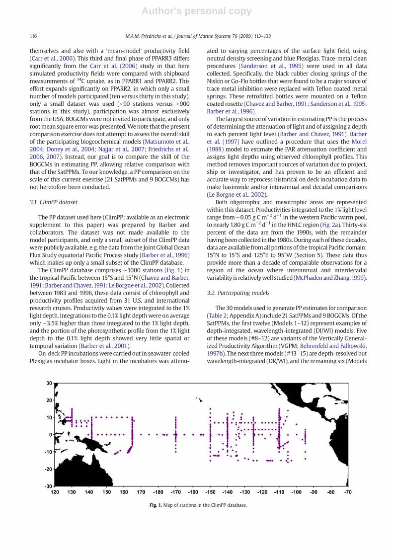
The ClimPP database comprises ∼1000 stations (Fig. 1) inthe tropical Pacific between 15°S and 15°N (Chavez and Barber,1991;Barber andChavez,1991; LeBorgneet al., 2002). Collectedbetween 1983 and 1996, these data consist of chlorophyll andproductivity profiles acquired from 31 U.S. and internationalresearch cruises. Productivity values were integrated to the 1%light depth. Integrations to the 0.1% light depthwere on averageonly ∼3.5% higher than those integrated to the 1% light depth,and the portion of the photosynthetic profile from the 1% lightdepth to the 0.1% light depth showed very little spatial ortemporal variation (Barber et al., 2001).
On-deck PP incubationswere carriedout in seawater-cooledPlexiglas incubator boxes. Light in the incubators was attenu-
ated to varying percentages of the surface light field, usingneutral density screening and blue Plexiglas. Trace-metal cleanprocedures (Sanderson et al., 1995) were used in all datacollected. Specifically, the black rubber closing springs of theNiskin or Go-Flo bottles that were found to be amajor source oftrace metal inhibition were replaced with Teflon coated metalsprings. These retrofitted bottles were mounted on a Tefloncoated rosette (Chavez and Barber,1991; Sanderson et al.,1995;Barber et al., 1996).
The largest sourceof variation in estimating PP is theprocessof determining the attenuation of light and of assigning a depthto each percent light level (Barber and Chavez, 1991). Barberet al. (1997) have outlined a procedure that uses the Morel(1988) model to estimate the PAR attenuation coefficient andassigns light depths using observed chlorophyll profiles. Thismethod removes important sources of variation due to project,ship or investigator, and has proven to be an efficient andaccurate way to reprocess historical on deck incubation data tomake basinwide and/or interannual and decadal comparisons(Le Borgne et al., 2002).
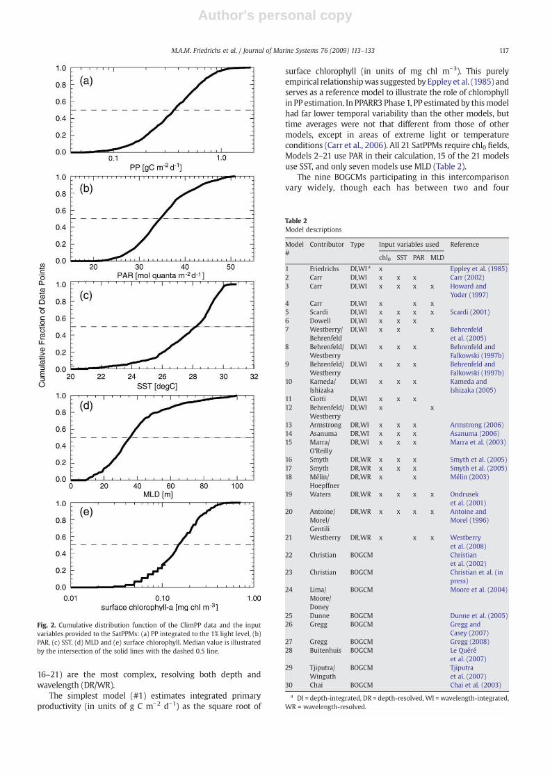
Both oligotrophic and mesotrophic areas are representedwithin this dataset. Productivities integrated to the 1% light levelrange from ∼0.05 g C m−2 d−1 in the western Pacific warm pool,to nearly 1.80 g Cm−2 d−1 in the HNLC region (Fig. 2a). Thirty-sixpercent of the data are from the 1990s, with the remainderhavingbeen collected in the1980s. Duringeachof thesedecades,data are available fromall portions of the tropical Pacificdomain:15°N to 15°S and 125°E to 95°W (Section 5). These data thusprovide more than a decade of comparable observations for aregion of the ocean where interannual and interdecadalvariability is relativelywell studied (McPhadenandZhang,1999).
3.2. Participating models
The30modelsused to generate PP estimates for comparison(Table 2;AppendixA) include21SatPPMsand9BOGCMs.Of theSatPPMs, the first twelve (Models 1–12) represent examples ofdepth-integrated, wavelength-integrated (DI/WI) models. Fiveof these models (#8–12) are variants of the Vertically General-ized Productivity Algorithm (VGPM; Behrenfeld and Falkowski,1997b). The next threemodels (#13–15) are depth-resolved butwavelength-integrated (DR/WI), and the remaining six (Models
Fig. 1. Map of stations in the ClimPP database.
116 M.A.M. Friedrichs et al. / Journal of Marine Systems 76 (2009) 113–133
Author's personal copy
16–21) are the most complex, resolving both depth andwavelength (DR/WR).
The simplest model (#1) estimates integrated primaryproductivity (in units of g C m−2 d−1) as the square root of
surface chlorophyll (in units of mg chl m−3). This purelyempirical relationshipwas suggested by Eppleyet al. (1985) andserves as a reference model to illustrate the role of chlorophyllin PP estimation. In PPARR3 Phase 1, PP estimated by thismodelhad far lower temporal variability than the other models, buttime averages were not that different from those of othermodels, except in areas of extreme light or temperatureconditions (Carr et al., 2006). All 21 SatPPMs require chl0 fields,Models 2–21 use PAR in their calculation, 15 of the 21 modelsuse SST, and only seven models use MLD (Table 2).
The nine BOGCMs participating in this intercomparisonvary widely, though each has between two and four
Fig. 2. Cumulative distribution function of the ClimPP data and the inputvariables provided to the SatPPMs: (a) PP integrated to the 1% light level, (b)PAR, (c) SST, (d) MLD and (e) surface chlorophyll. Median value is illustratedby the intersection of the solid lines with the dashed 0.5 line.
Table 2Model descriptions
Model#
Contributor Type Input variables used Reference
chl0 SST PAR MLD
1 Friedrichs DI,WI a x Eppley et al. (1985)2 Carr DI,WI x x x Carr (2002)3 Carr DI,WI x x x x Howard and
Yoder (1997)4 Carr DI,WI x x x5 Scardi DI,WI x x x x Scardi (2001)6 Dowell DI,WI x x x7 Westberry/
BehrenfeldDI,WI x x x Behrenfeld
et al. (2005)8 Behrenfeld/
WestberryDI,WI x x x Behrenfeld and
Falkowski (1997b)9 Behrenfeld/
WestberryDI,WI x x x Behrenfeld and
Falkowski (1997b)10 Kameda/
IshizakaDI,WI x x x Kameda and
Ishizaka (2005)11 Ciotti DI,WI x x x12 Behrenfeld/
WestberryDI,WI x x
13 Armstrong DR,WI x x x Armstrong (2006)14 Asanuma DR,WI x x x Asanuma (2006)15 Marra/
O'ReillyDR,WI x x x Marra et al. (2003)
16 Smyth DR,WR x x x Smyth et al. (2005)17 Smyth DR,WR x x x Smyth et al. (2005)18 Mélin/
HoepffnerDR,WR x x Mélin (2003)
19 Waters DR,WR x x x x Ondruseket al. (2001)
20 Antoine/Morel/Gentili
DR,WR x x x x Antoine andMorel (1996)
21 Westberry DR,WR x x x Westberryet al. (2008)
22 Christian BOGCM Christianet al. (2002)
23 Christian BOGCM Christian et al. (inpress)
24 Lima/Moore/Doney
BOGCM Moore et al. (2004)
25 Dunne BOGCM Dunne et al. (2005)26 Gregg BOGCM Gregg and
Casey (2007)27 Gregg BOGCM Gregg (2008)28 Buitenhuis BOGCM Le Quéré
et al. (2007)29 Tjiputra/
WinguthBOGCM Tjiputra
et al. (2007)30 Chai BOGCM Chai et al. (2003)
a DI = depth-integrated, DR = depth-resolved, WI = wavelength-integrated,WR = wavelength-resolved.
117M.A.M. Friedrichs et al. / Journal of Marine Systems 76 (2009) 113–133
Author's personal copy
phytoplankton functional groups, and each model containseither three or four nutrients. All BOGCMs except Model 29provide interannual, rather than climatological, PP distribu-tions. Although one BOGCM (#27) assimilates in situ NationalOcean Data Center chlorophyll data, none of the BOGCMsutilize any of the provided input fields (Table 2).
All 30 models provided estimates of productivity integratedto the 1% light level, for each of the ∼1000 ClimPP data points.Details regarding the structure of all 30participatingmodels arebeyond the scope of this paper, but key features of thesemodelsare provided in Table 2 and Appendix A. In addition, aforthcoming paper concentrates on identifying specific simila-rities and differences betweenmodel parameterizations, whichmay be affecting model performance (Saba et al., in prep.).
3.3. Input data variables for SatPPMs
Although none of themodelswere providedwith the PP data(Fig. 2a), the SatPPMs were provided with four types of inputvariables: daily mean chl0, PAR, SST, and MLD (Fig. 2b–e). Thesedata, along with the integrated productivities from the ClimPPdataset are included in this paperas anelectronic supplement. Asin PPARR2, chl0 was obtained from in situ data, rather thanremotely senseddata as inPPARR3Phase1.Although chlorophyllprofiles were available for each station, only the surface valueswere provided to the modelers. The profiles were used toestimate the depth of maximum chlorophyll (Section 5), but notprovided to the participants. NCEP/NCAR Reanalysis 1 data fordaily mean downward solar radiation flux data were down-loaded from theNational Oceanic&Atmospheric Administrationwebsite for the Physical Sciences Division of their Earth SystemResearch Laboratory. These NCEP/NCAR reanalysis data extendfrom1948until thepresent andareobtained froma state-of-the-art data assimilative analysis/forecast system. A factor of 0.43was used to convert these daily shortwave fluxes into PAR andproduced values that were in relatively good agreement(±10 mol quanta m−2 d−1) with PAR measurements obtainedon the Joint Global Ocean Flux Study equatorial Pacific ProcessStudy cruises. SST was obtained from the Advanced Very HighResolution Radiometer. MLD was obtained from a reduced-gravity, primitive equation tropical Pacific Oceanmodel (Murtu-gudde et al., 1996; Murtugudde and Busalacchi, 1998) with avariable depth mixed layer overlying 19 sigma layers. In thismodel, mixed layer thickness is determined using a “hybrid”mixed layer model (Chen et al., 1994) that considers both windstirring and shear instability, and produces interannual MLDestimates that are generally within ±20m of those derived frommeasurements collected on the Joint Global Ocean Flux Studyequatorial Pacific Process Study cruises.
Two models (e.g. Models 7 and 21) require information onparticulate backscatter at 443 nm (bbp), which is estimatedfrom ocean color remote sensing data (Maritorena et al., 2002).Since these data were not available for this pre-SeaWiFS eraClimPP dataset, monthly 9 km climatological bbp values (Sep.1997–Sep. 2007) were used for each given sample location.
3.4. Skill assessment strategies
The skill of the 30 participating models was assessed usingseveral strategies outlined below (also see Stowet al., 2009-thisvolume). Campbell et al. (2002) concluded in PPARR2 that the
total root mean square difference (RMSD) summed over the Ndata points provides a valuable comparison of PP models
RMSD ¼ 1N
∑N
i¼1Δ2
� �1=2
ð1Þ
Here model–data misfit in log10 space (Δ) is defined as:
Δ ið Þ ¼ log PPm ið Þð Þ−log PPd ið Þð Þwhere PPm(i) is modeled PP, obtained either via SatPPMs orBOGCMs, and PPd(i) represents the ClimPP data.
RMSD is composed of two components, the bias (B)representing the difference between the means of the twofields, and the centered pattern RMSD (RMSDCP; sometimesreferred to as the unbiased RMSD) representing the differ-ences in the variability of the two fields:
RMSD2 ¼ B2 þ RMSD2CP ð2Þ
The bias and RMSDCP (Tables 3 and 4) provide measures ofhow well the mean and variability are modeled, respectively:
B ¼ l̄og PPmð Þ− l̄og PPdð Þ ð3Þ
RMSDCP¼ 1N
∑Ni¼1 logPPm ið Þ− l̄ogPPm
� �− logPPd ið Þ− l̄ogPPd
� �� �2� �1=2
ð4Þ
Because the units of the above quantities are in decades oflog10 and not easily translated, a non-dimensional inversetransformed value for bias is presented:
Fmed ¼ 10B ð5Þwhere Fmed (Campbell et al., 2002) is the median value of theratio PPm ið Þ
PPd ið Þ ¼ 10Δi (Tables 3 and 4). Thus, if Fmed=2.0, themedian value of PPm(i) is a factor of two larger than themedian value of PPd(i); if Fmed=0.5, the median value of PPm(i) is a factor of two smaller than PPd(i).
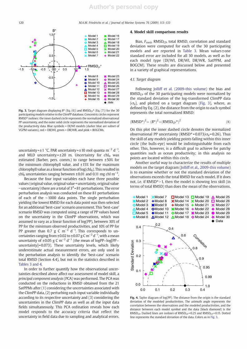
The novel target diagram (Jolliff et al., 2009-this volume) isused to visualize bias, RMSDCP, and total RMSD for the 30models on a single plot. On the target diagram, thesequantities are normalized by the standard deviation of logPPd(σd=0.279), i.e. normalized bias (B⁎) is defined as:
B⁎ ¼ B=σd; ð6Þ
Although RMSDCP is inherently a positive quantity,normalized RMSDCP (denoted as RMSDCP⁎) is defined as:
RMSDCP⁎ ¼ sign σm−σdð ÞRMSDCP=σd; ð7Þ
where σm is the standard deviation of logPPm, and thusRMSDCP⁎ can be either positive (indicating that the model isoverestimating the variance of the data) or negative (indicatingthat themodel is underestimating the variance of the data). It isimportant to note here that when the total RMSD statistic iscomputed, models that underestimate the observed variancetend to result in lower total RMSD scores than those thatoverestimate the variance (Jolliff et al., 2009-this volume).
For a given value of RMSDCP, a portion of the model–datamisfit will result fromphase differences between the simulatedand observed fields, and a portion will result from differences
118 M.A.M. Friedrichs et al. / Journal of Marine Systems 76 (2009) 113–133
Author's personal copy
between the amplitudes of the variations. Thus in addition toRMSDCP values, correlation coefficients and variances are alsocomputed (Tables 3 and 4) to understand the similarities anddifferences in model–data fit for each of the models participat-ing in this comparison. In Section 4.2 Taylor diagrams (Taylor,2001) are used to represent RMSDCP, correlation, and standarddeviation on a single plot.
The cumulative distribution function represents an alterna-tiveway to visualizemodel bias. Although B provides a succinctmeasure of the magnitude and sign of model bias, from thisstatistic alone it is not possible to determine whether positivebiases result from overestimating high values, or low values, orboth. A comparison of model and data cumulative distributionfunctions clearly reveals where in the spectrum of values thebiases occur, and is an excellentmethod for visualizingmedian,maximum and minimum values.
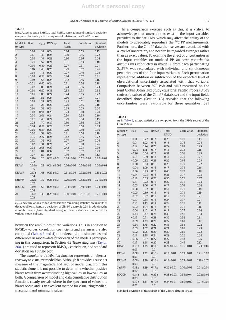
In a comparison exercise such as this, it is critical toacknowledge that uncertainties exist in the input variablesprovided to the SatPPMs, which may affect the ability of themodels to adequately reproduce the 14C PP measurements.Furthermore, the ClimPP data themselves are associated witha level of uncertainty and need to be regarded as ranges ratherthan as exact values. To examine the effect of uncertainties inthe input variables on modeled PP, an error perturbationanalysis was conducted in which PP from each participatingSatPPM was recalculated with individual and simultaneousperturbations of the four input variables. Each perturbationrepresented addition or subtraction of the expected level ofobservational uncertainty associated with that variable.Comparison between SST, PAR and MLD measured on theJoint Global Ocean Flux Study equatorial Pacific Process Studycruises (a subset of the ClimPP database) and the input fieldsdescribed above (Section 3.3) revealed that the followinguncertainties were reasonable for these quantities: SST
Table 4As in Table 3, except statistics are computed from the 1990s subset of theClimPP data
Model #or type
Bias Fmed RMSDCP TotalRMSD
Correlation Standarddeviation
1 −0.11 0.77 0.17 0.20 0.79 0.132 0.01 1.02 0.16 0.16 0.78 0.243 −0.12 0.74 0.20 0.24 0.67 0.254 0.04 1.11 0.17 0.18 0.72 0.185 −0.26 0.54 0.17 0.31 0.76 0.236 −0.01 0.99 0.18 0.18 0.78 0.277 −0.09 0.82 0.21 0.22 0.63 0.238 −0.20 0.64 0.16 0.25 0.77 0.229 0.04 1.09 0.16 0.17 0.78 0.1610 −0.36 0.43 0.17 0.40 0.72 0.1811 −0.14 0.73 0.16 0.21 0.77 0.2312 −0.19 0.65 0.23 0.30 0.79 0.3713 −0.15 0.72 0.16 0.22 0.78 0.2314 0.03 1.06 0.17 0.17 0.76 0.2415 −0.08 0.82 0.16 0.18 0.78 0.1816 −0.05 0.89 0.15 0.16 0.79 0.1917 −0.02 0.97 0.15 0.15 0.79 0.2118 −0.19 0.65 0.16 0.24 0.77 0.2119 0.15 1.43 0.18 0.24 0.75 0.1120 0.02 1.04 0.16 0.16 0.78 0.1621 0.04 1.10 0.17 0.18 0.75 0.2422 −0.33 0.47 0.28 0.43 0.59 0.3423 −0.15 0.71 0.28 0.32 0.52 0.3124 0.09 1.23 0.20 0.22 0.61 0.1725 0.24 1.75 0.22 0.33 0.58 0.2226 0.03 1.07 0.21 0.21 0.63 0.2327 0.02 1.05 0.20 0.20 0.64 0.2228 0.17 1.48 0.24 0.29 0.26 0.0629 −0.06 0.87 0.27 0.27 0.44 0.2630 0.17 1.48 0.22 0.28 0.46 0.12DI/WI 0.13±
0.031.35 0.18±
0.010.24±0.02 0.75±0.01 0.23±0.02
DR/WI 0.08±0.03
1.22 0.16±0.01
0.19±0.01 0.77±0.01 0.21±0.02
DR/WR 0.08±0.03
1.20 0.16±0.01
0.19±0.02 0.77±0.01 0.19±0.02
SatPPM 0.11±0.02
1.29 0.17±0.01
0.22±0.01 0.76±0.01 0.21±0.01
BOGCM 0.14±0.03
1.38 0.23±0.01
0.28±0.02 0.53±0.04 0.22±0.03
All 0.12±0.02
1.31 0.19±0.01
0.24±0.01 0.69±0.02 0.21±0.01
Standard deviation of this subset of the ClimPP dataset is 0.25.
Table 3Bias, Fmed (see text), RMSDCP, total RMSD, correlation and standard deviationcomputed for each participating model relative to the ClimPP dataset
Model #or type
Bias Fmed RMSDCP TotalRMSD
Correlation Standarddeviation
1 0.04 1.10 0.24 0.24 0.53 0.132 0.17 1.48 0.24 0.30 0.55 0.223 0.04 1.10 0.29 0.30 0.36 0.244 0.20 1.57 0.24 0.31 0.53 0.185 −0.09 0.80 0.25 0.27 0.51 0.216 0.16 1.43 0.25 0.29 0.57 0.267 0.05 1.13 0.27 0.27 0.49 0.258 −0.04 0.92 0.24 0.24 0.57 0.219 0.19 1.56 0.25 0.32 0.46 0.1610 −0.21 0.62 0.24 0.31 0.54 0.1811 0.02 1.06 0.24 0.24 0.56 0.2312 −0.01 0.97 0.33 0.33 0.53 0.3813 0.01 1.03 0.24 0.24 0.55 0.2214 0.18 1.53 0.24 0.30 0.57 0.2115 0.07 1.18 0.24 0.25 0.51 0.1816 0.11 1.28 0.23 0.26 0.55 0.1817 0.14 1.39 0.24 0.28 0.53 0.2018 −0.04 0.91 0.23 0.23 0.60 0.2019 0.30 2.01 0.24 0.39 0.55 0.1020 0.17 1.48 0.24 0.29 0.54 0.1521 0.25 1.79 0.30 0.39 0.36 0.2622 −0.24 0.58 0.29 0.37 0.56 0.3323 −0.05 0.89 0.29 0.29 0.50 0.3024 0.20 1.58 0.24 0.31 0.54 0.1925 0.35 2.22 0.24 0.42 0.55 0.2226 0.12 1.33 0.24 0.27 0.59 0.2627 0.12 1.31 0.24 0.27 0.60 0.2628 0.32 2.08 0.27 0.42 0.23 0.0829 0.00 1.01 0.32 0.32 0.37 0.2930 0.27 1.87 0.24 0.36 0.50 0.12DI/WI 0.10±
0.021.26 0.26±0.01 0.28±0.01 0.52±0.02 0.22±0.02
DR/WI 0.09±0.05
1.23 0.24±0.002 0.26±0.02 0.54±0.02 0.20±0.01
DR/WR 0.17±0.04
1.48 0.25±0.01 0.31±0.03 0.52±0.03 0.18±0.02
SatPPM 0.12±0.02
1.32 0.25±0.01 0.29±0.01 0.52±0.01 0.21±0.01
BOGCM 0.19±0.04
1.53 0.26±0.01 0.34±0.02 0.49±0.04 0.23±0.03
All 0.14±0.02
1.38 0.25±0.01 0.30±0.01 0.51±0.01 0.21±0.01
Fmed and correlation are non-dimensional; remaining statistics are in units ofdecades of log10. Standard deviation of ClimPP dataset is 0.28. In addition, theabsolute means (±one standard error) of these statistics are reported forvarious model subsets.
119M.A.M. Friedrichs et al. / Journal of Marine Systems 76 (2009) 113–133
Author's personal copy
uncertainty=±1 °C, PAR uncertainty=±10 mol quanta m−2 d−1,and MLD uncertainty=±20 m. Uncertainty for chl0 wasestimated (Barber, pers. comm.) to range between ±50% forthe minimum chlorophyll value, and ±15% for the maximumchlorophyll value asa linear functionof log(chl0). This resulted inchl0 uncertainties ranging between ±0.01 and 0.11 mg chl m−3.
Because the four input variables each have three possiblevalues (original value, original value+uncertainty, original value−uncertainty) there are a total of 34=81 perturbations. Theerrorperturbation analysis was conducted on these 81 perturbationsof each of the ∼1000 data points. The single perturbationyielding the lowest RMSD for each data point was then selectedfor anadditional ‘best-case’ scenario assessment. This ‘best-case’scenario RMSD was computed using a range of PP values basedon the uncertainty in the ClimPP observations, which wasassumed to vary as a linear function of log(PP), between 30% ofPP for the minimum observed productivities, and 10% of PP forPP greater than 0.7 g C m−2 d−1. This corresponds to un-certainties ranging from±0.02 to ±0.07 g Cm−2 d−1,with ameanuncertainty of ±0.05 g C m−2 d−1 (the mean of logPP–log[PP–uncertainty]=0.073). These uncertainty levels, which likelyunderestimate actual measurement errors, are only used inthe perturbation analysis to identify the ‘best-case’ scenariototal RMSD (Section 4.4), but not in the statistics described inTables 3 and 4.
In order to further quantify how the observational uncer-tainties described above affect our assessment of model skill, aprincipal component analysis (PCA)was performed. The PCAwasconducted on the reductions in RMSD obtained from the 21SatPPMs after (1) considering the uncertainties associated withthe ClimPP data, (2) perturbing each input variable individuallyaccording to its respective uncertainty and (3) considering theuncertainties in the ClimPP data as well as all the input datafields simultaneously. This PCA ordination reveals how eachmodel responds to the accuracy criteria that reflect theuncertainty in field data due to sampling and analytical errors.
4. Model skill comparison results
Bias, Fmed, RMSDCP, total RMSD, correlation and standarddeviation were computed for each of the 30 participatingmodels and are reported in Table 3. Mean values±onestandard error are included for all 30 models, as well as foreach model type (DI/WI, DR/WI, DR/WR, SatPPM, andBOGCM). These results are discussed below and presentedin a variety of graphical representations.
4.1. Target diagram
Following Jolliff et al. (2009-this volume) the bias andRMSDCP of the 30 participating models were normalized bythe standard deviation of the log-transformed ClimPP data(σd), and plotted on a target diagram (Fig. 3), where, asdefined by Eq. (2), the distance from the origin to each symbolrepresents the total normalized RMSD:
RMSD⁎ð Þ2¼ B⁎ð Þ2þ RMSDCP⁎ð Þ2 ð8ÞOn this plot the inner dashed circle denotes the normalizedobservational PP uncertainty (RMSD⁎=0.073/σd=0.26). Thusthe skill of anymodels yielding points fallingwithin this innercircle (the bulls-eye) would be indistinguishable from eachother. This, however, is a difficult goal to achieve for patchyquantities such as ocean productivity; in this analysis nopoints are located within this circle.
Another useful way to characterize the results of multiplemodels on the target diagram (Jolliff et al., 2009-this volume)is to examine whether or not the standard deviation of theobservations exceeds the total RMSD for each model. If it doesnot, i.e. if RMSD⁎N1, then the model is showing less skill (interms of total RMSD) than does the mean of the observations.
Fig. 3. Target diagram displaying B⁎ (Eq. (6)) and RMSDCP⁎ (Eq. (7)) for the 30participatingmodels relative to theClimPPdatabase. Concentric circles representRMSD⁎ isolines: the inner dashed circle represents the normalized observationalPP uncertainty, and the outer solid circle represents the normalized deviation ofthe productivity data. Blue symbols = DI/WI models (darker blue are subset ofVGPM variants), red = DR/WI, green = DR/WR, and pink = BOGCMs.
Fig. 4. Taylor diagram of log(PP). The distance from the origin is the standarddeviation of the modeled productivities. The azimuth angle represents thecorrelation between the observations and the modeled productivities, and thedistance between each model symbol and the data (black diamond) is theRMSDCP. Dashed lines are isolines of RMSDCP=0.25 and RMSDCP=0.15. Dottedline represents the standard deviation of the data. Colors as in Fig. 3.
120 M.A.M. Friedrichs et al. / Journal of Marine Systems 76 (2009) 113–133
Author's personal copy
Model results falling inside the outer circle, i.e. those withtotal RMSD values that are less than the standard deviation ofthe observations, tend to provide a better instantaneousestimate of productivity than the mean of the observations. Inthis analysis, eleven of the 30 models (37%) fell within thisouter circle (Fig. 3). These include 42% of the DI/WI models,67% of the DR/WI models, 33% of the DR/WR models and 22%of the BOGCMs. The model with the lowest normalized totalRMSD (RMSD⁎=0.82) is Model 18, a DR/WR model. Fourmodels have nearly equally low RMSD: two VGPM variants(Models 8 and 11), a depth-resolved model (Model 13) andthe simplistic sqrt(chl0) relationship (Model 1). The perfor-mance of the latter model, which does not use PAR, SST orMLD data, illustrates the importance of chl0 in the estimationof integrated productivity.
The target diagram (Fig. 3) also illustrates that most (23out of 30) models overestimated observed productivity(B⁎N0), whereas only 23% (7 out of 30) models under-estimated productivity. Three models (one SatPPM #19, andtwo BOGCMs #25, 28) had positive median biases greaterthan two (FmedN2.0; BN0.3; Table 3), i.e. in these cases themedian modeled value was more than twice the medianobserved value. Nearly half of the BOGCMs (four of nine) wereassociated with absolute biases greater than a factor of 1.7(FmedN1.7 or Fmedb0.59), whereas only two of the 21 SatPPMs,both DR/WR models, were associated with biases of thismagnitude. Interestingly, the overall magnitude of the meanbias was lower for the DI/WI models (0.10±0.02) than for theDR/WR models (0.17±0.04) and the BOGCMs (0.19±0.02).
The centered pattern RMSD (RMSDCP) provides a measureof how well the variability of a certain field is being modeled.Whereas bias for these models varied substantially, themagnitude of RMSDCP diverged much less among models(Table 3), ranging only from |RMSDCP⁎|=0.84 to 1.13 (Fig. 3).The RMSDCP was slightly, but not significantly, higher for theBOGCMs (j¯RMSD⁎
CP j=0.95±0.04) than for the SatPPMs(j¯RMSD⁎
CP j=0.90±0.02). There was also little significantdifference in j¯RMSD⁎
CP j for the different categories ofSatPPMs. All but four models (three BOGCMS and oneVGPM variant) underestimated the variance of observedproductivity (RMSDCP⁎b0).
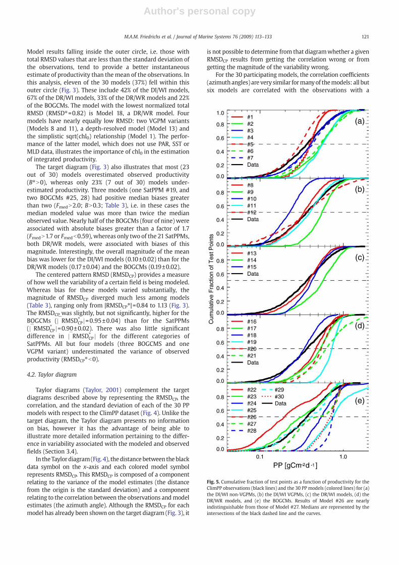
4.2. Taylor diagram
Taylor diagrams (Taylor, 2001) complement the targetdiagrams described above by representing the RMSDCP, thecorrelation, and the standard deviation of each of the 30 PPmodels with respect to the ClimPP dataset (Fig. 4). Unlike thetarget diagram, the Taylor diagram presents no informationon bias, however it has the advantage of being able toillustrate more detailed information pertaining to the differ-ence in variability associated with the modeled and observedfields (Section 3.4).
In theTaylordiagram(Fig. 4), thedistance between theblackdata symbol on the x-axis and each colored model symbolrepresents RMSDCP. This RMSDCP is composed of a componentrelating to the variance of the model estimates (the distancefrom the origin is the standard deviation) and a componentrelating to the correlation between the observations andmodelestimates (the azimuth angle). Although the RMSDCP for eachmodel has already been shown on the target diagram (Fig. 3), it
is not possible to determine from that diagramwhether a givenRMSDCP results from getting the correlation wrong or fromgetting the magnitude of the variability wrong.
For the 30 participating models, the correlation coefficients(azimuthangles) are very similar formanyof themodels: all butsix models are correlated with the observations with a
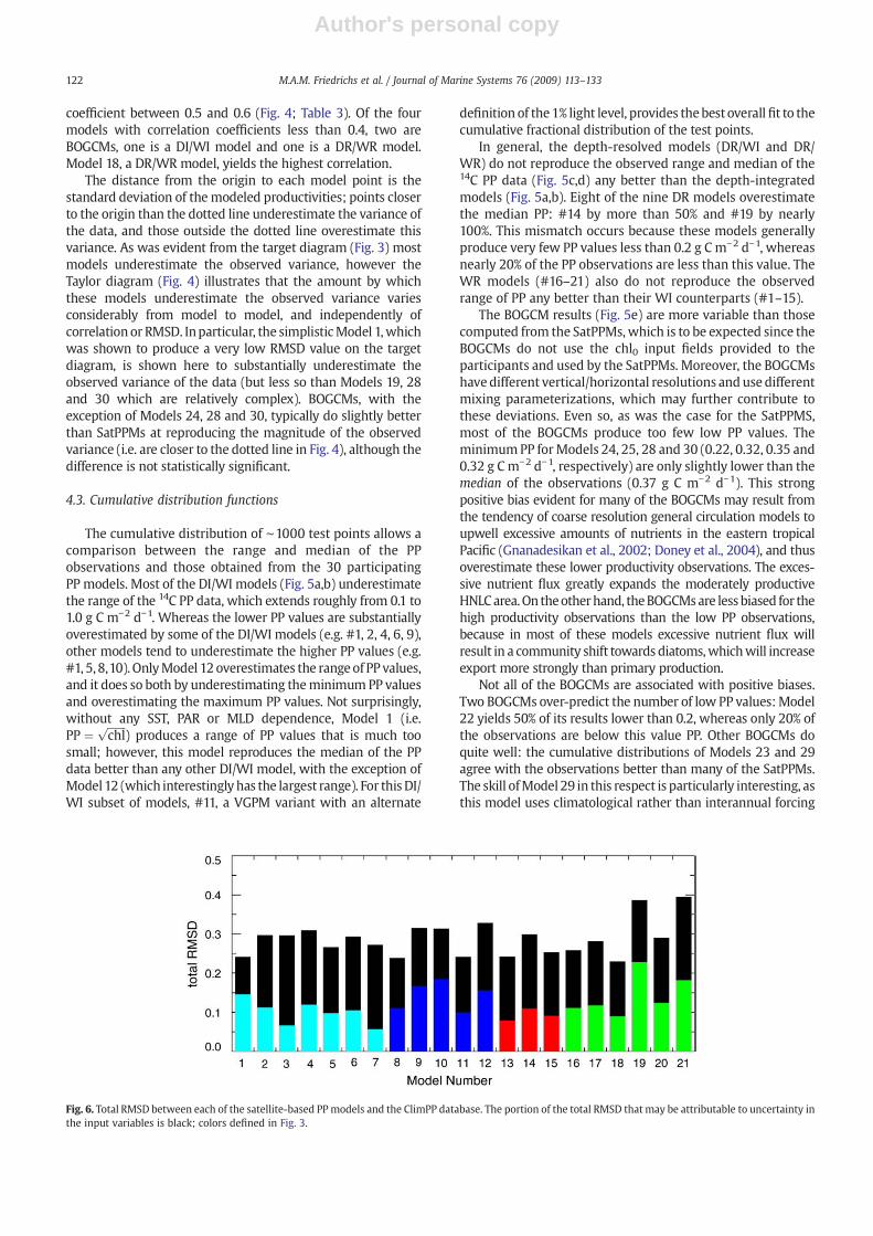
Fig. 5. Cumulative fraction of test points as a function of productivity for theClimPP observations (black lines) and the 30 PP models (colored lines) for (a)the DI/WI non-VGPMs, (b) the DI/WI VGPMs, (c) the DR/WI models, (d) theDR/WR models, and (e) the BOGCMs. Results of Model #26 are nearlyindistinguishable from those of Model #27. Medians are represented by theintersections of the black dashed line and the curves.
121M.A.M. Friedrichs et al. / Journal of Marine Systems 76 (2009) 113–133
Author's personal copy
coefficient between 0.5 and 0.6 (Fig. 4; Table 3). Of the fourmodels with correlation coefficients less than 0.4, two areBOGCMs, one is a DI/WI model and one is a DR/WR model.Model 18, a DR/WR model, yields the highest correlation.
The distance from the origin to each model point is thestandard deviation of themodeled productivities; points closerto the origin than the dotted line underestimate the variance ofthe data, and those outside the dotted line overestimate thisvariance. As was evident from the target diagram (Fig. 3) mostmodels underestimate the observed variance, however theTaylor diagram (Fig. 4) illustrates that the amount by whichthese models underestimate the observed variance variesconsiderably from model to model, and independently ofcorrelation or RMSD. Inparticular, the simplisticModel 1,whichwas shown to produce a very low RMSD value on the targetdiagram, is shown here to substantially underestimate theobserved variance of the data (but less so than Models 19, 28and 30 which are relatively complex). BOGCMs, with theexception of Models 24, 28 and 30, typically do slightly betterthan SatPPMs at reproducing the magnitude of the observedvariance (i.e. are closer to the dotted line in Fig. 4), although thedifference is not statistically significant.
4.3. Cumulative distribution functions
The cumulative distribution of ∼1000 test points allows acomparison between the range and median of the PPobservations and those obtained from the 30 participatingPP models. Most of the DI/WI models (Fig. 5a,b) underestimatethe range of the 14C PP data, which extends roughly from 0.1 to1.0 g C m−2 d−1. Whereas the lower PP values are substantiallyoverestimated by some of the DI/WI models (e.g. #1, 2, 4, 6, 9),other models tend to underestimate the higher PP values (e.g.#1, 5, 8,10). OnlyModel 12 overestimates the rangeof PP values,and it does so both by underestimating theminimum PP valuesand overestimating the maximum PP values. Not surprisingly,without any SST, PAR or MLD dependence, Model 1 (i.e.PP ¼
ffiffiffiffiffiffiffichl
p) produces a range of PP values that is much too
small; however, this model reproduces the median of the PPdata better than any other DI/WI model, with the exception ofModel12 (which interestingly has the largest range). For thisDI/WI subset of models, #11, a VGPM variant with an alternate
definition of the1% light level, provides thebest overallfit to thecumulative fractional distribution of the test points.
In general, the depth-resolved models (DR/WI and DR/WR) do not reproduce the observed range and median of the14C PP data (Fig. 5c,d) any better than the depth-integratedmodels (Fig. 5a,b). Eight of the nine DR models overestimatethe median PP: #14 by more than 50% and #19 by nearly100%. This mismatch occurs because these models generallyproduce very few PP values less than 0.2 g C m−2 d−1, whereasnearly 20% of the PP observations are less than this value. TheWR models (#16–21) also do not reproduce the observedrange of PP any better than their WI counterparts (#1–15).
The BOGCM results (Fig. 5e) are more variable than thosecomputed from the SatPPMs,which is to be expected since theBOGCMs do not use the chl0 input fields provided to theparticipants and used by the SatPPMs. Moreover, the BOGCMshavedifferent vertical/horizontal resolutions and use differentmixing parameterizations, which may further contribute tothese deviations. Even so, as was the case for the SatPPMS,most of the BOGCMs produce too few low PP values. TheminimumPP forModels 24, 25, 28 and 30 (0.22, 0.32, 0.35 and0.32 g Cm−2 d−1, respectively) are only slightly lower than themedian of the observations (0.37 g C m−2 d−1). This strongpositive bias evident for many of the BOGCMs may result fromthe tendency of coarse resolution general circulation models toupwell excessive amounts of nutrients in the eastern tropicalPacific (Gnanadesikan et al., 2002; Doney et al., 2004), and thusoverestimate these lower productivity observations. The exces-sive nutrient flux greatly expands the moderately productiveHNLCarea.On theotherhand, theBOGCMsare less biased for thehigh productivity observations than the low PP observations,because in most of these models excessive nutrient flux willresult in a community shift towards diatoms,whichwill increaseexport more strongly than primary production.
Not all of the BOGCMs are associated with positive biases.Two BOGCMs over-predict the number of low PP values:Model22 yields 50% of its results lower than 0.2, whereas only 20% ofthe observations are below this value PP. Other BOGCMs doquite well: the cumulative distributions of Models 23 and 29agree with the observations better than many of the SatPPMs.The skill ofModel 29 in this respect is particularly interesting, asthis model uses climatological rather than interannual forcing
Fig. 6. Total RMSD between each of the satellite-based PPmodels and the ClimPP database. The portion of the total RMSD that may be attributable to uncertainty inthe input variables is black; colors defined in Fig. 3.
122 M.A.M. Friedrichs et al. / Journal of Marine Systems 76 (2009) 113–133
Author's personal copy
fields. Overall, the performance of the BOGCMs varies substan-tially, and as a group ofmodels they do notmatch the range andmedian of the observed PP any better or worse than theSatPPMs.
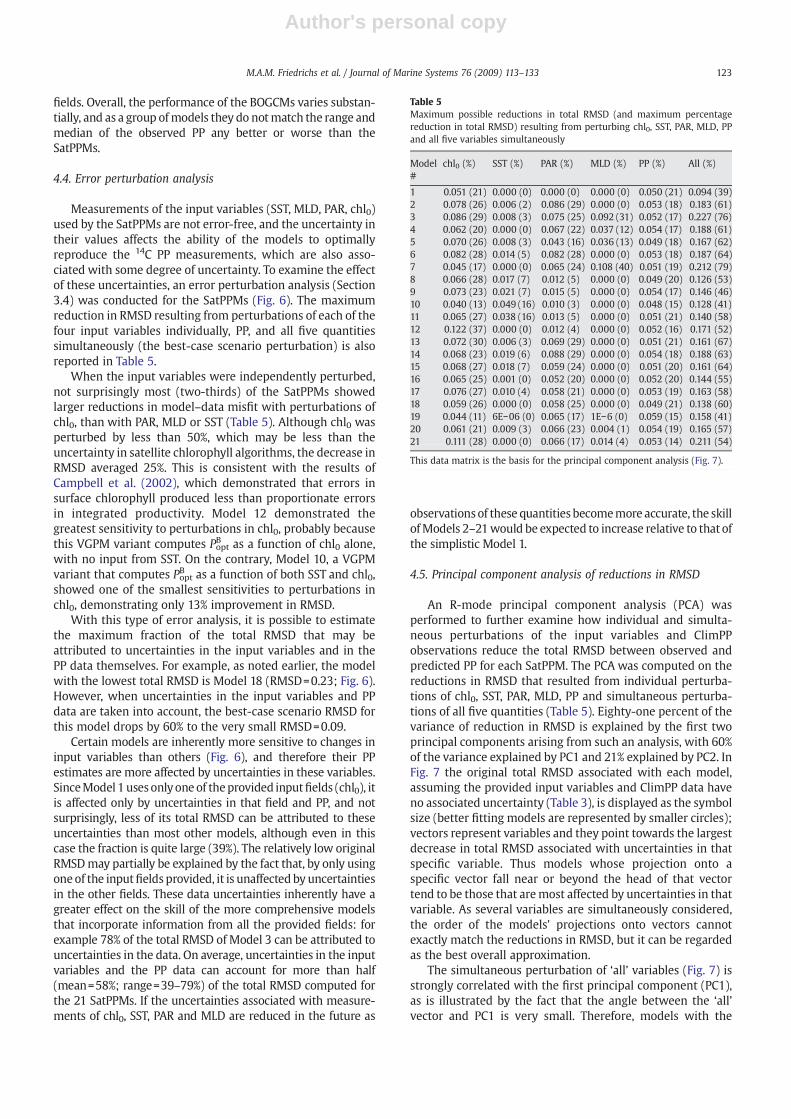
4.4. Error perturbation analysis
Measurements of the input variables (SST, MLD, PAR, chl0)used by the SatPPMs are not error-free, and the uncertainty intheir values affects the ability of the models to optimallyreproduce the 14C PP measurements, which are also asso-ciated with some degree of uncertainty. To examine the effectof these uncertainties, an error perturbation analysis (Section3.4) was conducted for the SatPPMs (Fig. 6). The maximumreduction in RMSD resulting from perturbations of each of thefour input variables individually, PP, and all five quantitiessimultaneously (the best-case scenario perturbation) is alsoreported in Table 5.
When the input variables were independently perturbed,not surprisingly most (two-thirds) of the SatPPMs showedlarger reductions in model–data misfit with perturbations ofchl0, than with PAR, MLD or SST (Table 5). Although chl0 wasperturbed by less than 50%, which may be less than theuncertainty in satellite chlorophyll algorithms, the decrease inRMSD averaged 25%. This is consistent with the results ofCampbell et al. (2002), which demonstrated that errors insurface chlorophyll produced less than proportionate errorsin integrated productivity. Model 12 demonstrated thegreatest sensitivity to perturbations in chl0, probably becausethis VGPM variant computes Popt
B as a function of chl0 alone,with no input from SST. On the contrary, Model 10, a VGPMvariant that computes PoptB as a function of both SST and chl0,showed one of the smallest sensitivities to perturbations inchl0, demonstrating only 13% improvement in RMSD.
With this type of error analysis, it is possible to estimatethe maximum fraction of the total RMSD that may beattributed to uncertainties in the input variables and in thePP data themselves. For example, as noted earlier, the modelwith the lowest total RMSD is Model 18 (RMSD=0.23; Fig. 6).However, when uncertainties in the input variables and PPdata are taken into account, the best-case scenario RMSD forthis model drops by 60% to the very small RMSD=0.09.
Certain models are inherently more sensitive to changes ininput variables than others (Fig. 6), and therefore their PPestimates are more affected by uncertainties in these variables.SinceModel 1 usesonlyoneof theprovided inputfields (chl0), itis affected only by uncertainties in that field and PP, and notsurprisingly, less of its total RMSD can be attributed to theseuncertainties than most other models, although even in thiscase the fraction is quite large (39%). The relatively low originalRMSDmay partially be explained by the fact that, by only usingoneof the inputfields provided, it is unaffected by uncertaintiesin the other fields. These data uncertainties inherently have agreater effect on the skill of the more comprehensive modelsthat incorporate information from all the provided fields: forexample 78% of the total RMSD of Model 3 can be attributed touncertainties in the data. On average, uncertainties in the inputvariables and the PP data can account for more than half(mean=58%; range=39–79%) of the total RMSD computed forthe 21 SatPPMs. If the uncertainties associated with measure-ments of chl0, SST, PAR and MLD are reduced in the future as
observationsof these quantities becomemore accurate, the skillofModels 2–21would be expected to increase relative to that ofthe simplistic Model 1.
4.5. Principal component analysis of reductions in RMSD
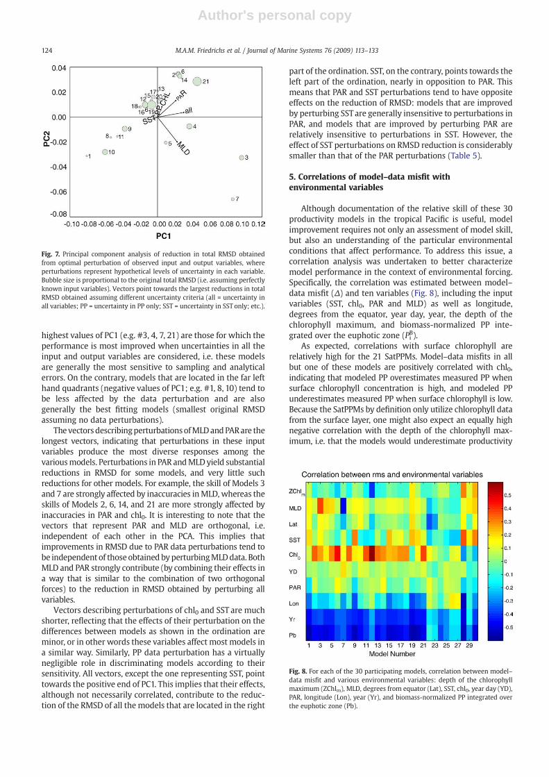
An R-mode principal component analysis (PCA) wasperformed to further examine how individual and simulta-neous perturbations of the input variables and ClimPPobservations reduce the total RMSD between observed andpredicted PP for each SatPPM. The PCA was computed on thereductions in RMSD that resulted from individual perturba-tions of chl0, SST, PAR, MLD, PP and simultaneous perturba-tions of all five quantities (Table 5). Eighty-one percent of thevariance of reduction in RMSD is explained by the first twoprincipal components arising from such an analysis, with 60%of the variance explained by PC1 and 21% explained by PC2. InFig. 7 the original total RMSD associated with each model,assuming the provided input variables and ClimPP data haveno associated uncertainty (Table 3), is displayed as the symbolsize (better fitting models are represented by smaller circles);vectors represent variables and they point towards the largestdecrease in total RMSD associated with uncertainties in thatspecific variable. Thus models whose projection onto aspecific vector fall near or beyond the head of that vectortend to be those that aremost affected by uncertainties in thatvariable. As several variables are simultaneously considered,the order of the models' projections onto vectors cannotexactly match the reductions in RMSD, but it can be regardedas the best overall approximation.
The simultaneous perturbation of ‘all’ variables (Fig. 7) isstrongly correlated with the first principal component (PC1),as is illustrated by the fact that the angle between the ‘all’vector and PC1 is very small. Therefore, models with the
Table 5Maximum possible reductions in total RMSD (and maximum percentagereduction in total RMSD) resulting from perturbing chl0, SST, PAR, MLD, PPand all five variables simultaneously
Model#
chl0 (%) SST (%) PAR (%) MLD (%) PP (%) All (%)
1 0.051 (21) 0.000 (0) 0.000 (0) 0.000 (0) 0.050 (21) 0.094 (39)2 0.078 (26) 0.006 (2) 0.086 (29) 0.000 (0) 0.053 (18) 0.183 (61)3 0.086 (29) 0.008 (3) 0.075 (25) 0.092 (31) 0.052 (17) 0.227 (76)4 0.062 (20) 0.000 (0) 0.067 (22) 0.037 (12) 0.054 (17) 0.188 (61)5 0.070 (26) 0.008 (3) 0.043 (16) 0.036 (13) 0.049 (18) 0.167 (62)6 0.082 (28) 0.014 (5) 0.082 (28) 0.000 (0) 0.053 (18) 0.187 (64)7 0.045 (17) 0.000 (0) 0.065 (24) 0.108 (40) 0.051 (19) 0.212 (79)8 0.066 (28) 0.017 (7) 0.012 (5) 0.000 (0) 0.049 (20) 0.126 (53)9 0.073 (23) 0.021 (7) 0.015 (5) 0.000 (0) 0.054 (17) 0.146 (46)10 0.040 (13) 0.049 (16) 0.010 (3) 0.000 (0) 0.048 (15) 0.128 (41)11 0.065 (27) 0.038 (16) 0.013 (5) 0.000 (0) 0.051 (21) 0.140 (58)12 0.122 (37) 0.000 (0) 0.012 (4) 0.000 (0) 0.052 (16) 0.171 (52)13 0.072 (30) 0.006 (3) 0.069 (29) 0.000 (0) 0.051 (21) 0.161 (67)14 0.068 (23) 0.019 (6) 0.088 (29) 0.000 (0) 0.054 (18) 0.188 (63)15 0.068 (27) 0.018 (7) 0.059 (24) 0.000 (0) 0.051 (20) 0.161 (64)16 0.065 (25) 0.001 (0) 0.052 (20) 0.000 (0) 0.052 (20) 0.144 (55)17 0.076 (27) 0.010 (4) 0.058 (21) 0.000 (0) 0.053 (19) 0.163 (58)18 0.059 (26) 0.000 (0) 0.058 (25) 0.000 (0) 0.049 (21) 0.138 (60)19 0.044 (11) 6E−06 (0) 0.065 (17) 1E−6 (0) 0.059 (15) 0.158 (41)20 0.061 (21) 0.009 (3) 0.066 (23) 0.004 (1) 0.054 (19) 0.165 (57)21 0.111 (28) 0.000 (0) 0.066 (17) 0.014 (4) 0.053 (14) 0.211 (54)
This data matrix is the basis for the principal component analysis (Fig. 7).
123M.A.M. Friedrichs et al. / Journal of Marine Systems 76 (2009) 113–133
Author's personal copy
highest values of PC1 (e.g. #3, 4, 7, 21) are those for which theperformance is most improved when uncertainties in all theinput and output variables are considered, i.e. these modelsare generally the most sensitive to sampling and analyticalerrors. On the contrary, models that are located in the far lefthand quadrants (negative values of PC1; e.g. #1, 8, 10) tend tobe less affected by the data perturbation and are alsogenerally the best fitting models (smallest original RMSDassuming no data perturbations).
Thevectors describingperturbationsofMLDandPARare thelongest vectors, indicating that perturbations in these inputvariables produce the most diverse responses among thevariousmodels. Perturbations in PAR andMLD yield substantialreductions in RMSD for some models, and very little suchreductions for other models. For example, the skill of Models 3and 7 are strongly affected by inaccuracies inMLD, whereas theskills of Models 2, 6, 14, and 21 are more strongly affected byinaccuracies in PAR and chl0. It is interesting to note that thevectors that represent PAR and MLD are orthogonal, i.e.independent of each other in the PCA. This implies thatimprovements in RMSD due to PAR data perturbations tend tobe independent of those obtained byperturbingMLDdata. BothMLD and PAR strongly contribute (by combining their effects ina way that is similar to the combination of two orthogonalforces) to the reduction in RMSD obtained by perturbing allvariables.
Vectors describing perturbations of chl0 and SST are muchshorter, reflecting that the effects of their perturbation on thedifferences between models as shown in the ordination areminor, or in other words these variables affect most models ina similar way. Similarly, PP data perturbation has a virtuallynegligible role in discriminating models according to theirsensitivity. All vectors, except the one representing SST, pointtowards the positive end of PC1. This implies that their effects,although not necessarily correlated, contribute to the reduc-tion of the RMSD of all the models that are located in the right
part of the ordination. SST, on the contrary, points towards theleft part of the ordination, nearly in opposition to PAR. Thismeans that PAR and SST perturbations tend to have oppositeeffects on the reduction of RMSD: models that are improvedby perturbing SST are generally insensitive to perturbations inPAR, and models that are improved by perturbing PAR arerelatively insensitive to perturbations in SST. However, theeffect of SST perturbations on RMSD reduction is considerablysmaller than that of the PAR perturbations (Table 5).
5. Correlations of model–data misfit withenvironmental variables
Although documentation of the relative skill of these 30productivity models in the tropical Pacific is useful, modelimprovement requires not only an assessment of model skill,but also an understanding of the particular environmentalconditions that affect performance. To address this issue, acorrelation analysis was undertaken to better characterizemodel performance in the context of environmental forcing.Specifically, the correlation was estimated between model–data misfit (Δ) and ten variables (Fig. 8), including the inputvariables (SST, chl0, PAR and MLD) as well as longitude,degrees from the equator, year day, year, the depth of thechlorophyll maximum, and biomass-normalized PP inte-grated over the euphotic zone (PiB).
As expected, correlations with surface chlorophyll arerelatively high for the 21 SatPPMs. Model–data misfits in allbut one of these models are positively correlated with chl0,indicating that modeled PP overestimates measured PP whensurface chlorophyll concentration is high, and modeled PPunderestimates measured PP when surface chlorophyll is low.Because the SatPPMs by definition only utilize chlorophyll datafrom the surface layer, one might also expect an equally highnegative correlation with the depth of the chlorophyll max-imum, i.e. that the models would underestimate productivity
Fig. 8. For each of the 30 participating models, correlation between model–data misfit and various environmental variables: depth of the chlorophyllmaximum (ZChlm), MLD, degrees from equator (Lat), SST, chl0, year day (YD),PAR, longitude (Lon), year (Yr), and biomass-normalized PP integrated overthe euphotic zone (Pb).
Fig. 7. Principal component analysis of reduction in total RMSD obtainedfrom optimal perturbation of observed input and output variables, whereperturbations represent hypothetical levels of uncertainty in each variable.Bubble size is proportional to the original total RMSD (i.e. assuming perfectlyknown input variables). Vectors point towards the largest reductions in totalRMSD obtained assuming different uncertainty criteria (all = uncertainty inall variables; PP = uncertainty in PP only; SST = uncertainty in SST only; etc.).
124 M.A.M. Friedrichs et al. / Journal of Marine Systems 76 (2009) 113–133
Author's personal copy
when themaximum chlorophyll concentration occurred belowone optical depth. Because large parts of this region arecharacterized by deep chlorophyll maxima (Barber et al.,1996; Le Borgne et al., 2002), the ClimPP dataset provides agood test of the impact of chlorophyll vertical structure onmodel misfit. However, Fig. 8 illustrates that the correlationbetween misfit and the depth of the chlorophyll maximum isgenerally less than 0.1. Only Model 12 produced misfits thatwere strongly correlated to the depth of the chlorophyllmaximum, overestimating the ClimPP data when the max-imum chlorophyll concentrationwas at the surface and under-estimating the ClimPP data when the maximum chlorophyllconcentration was deep. This latter behavior is what would beexpected from models that use only a surface value, and hasbeen a concern for the use of ocean color. The low correlationbetween misfit and depth of the chlorophyll maximum for thebulk of the models suggests that model assumptions typicallyused to characterize the depth profile of chlorophyll are fairlysound, and/or that the variations of PP in the deep chlorophyllmaximumdonot contribute strongly to vertically integrated PP.
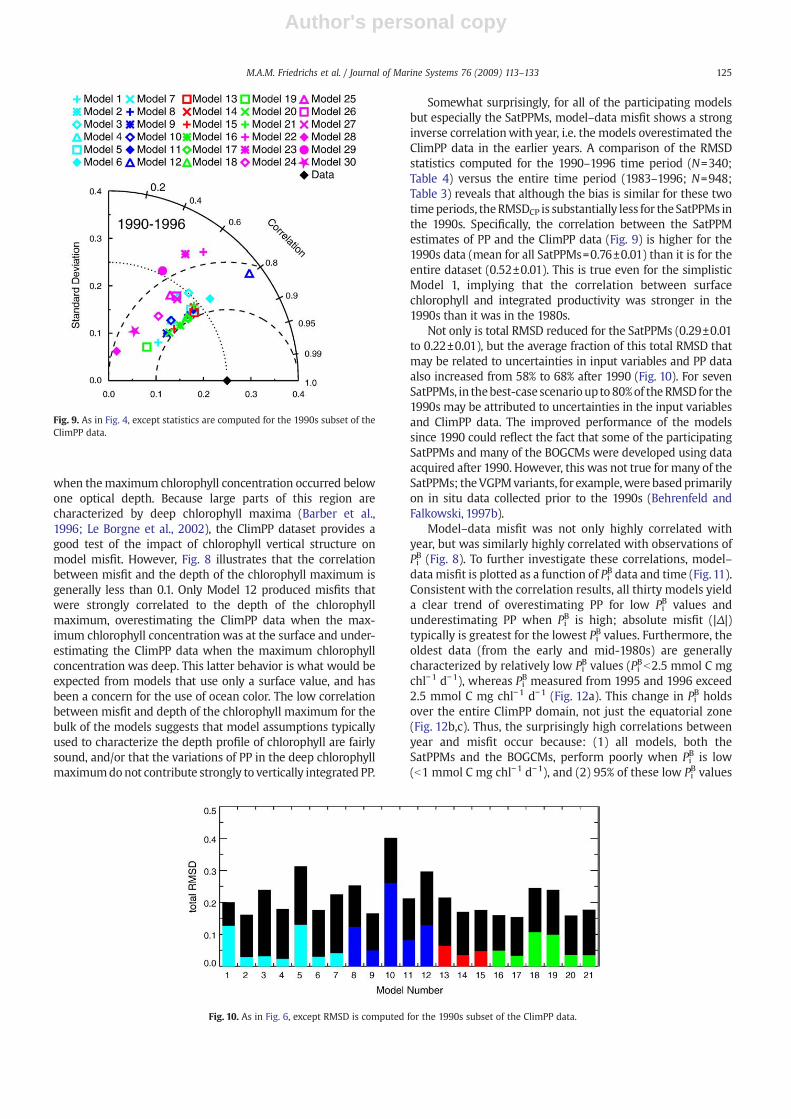
Somewhat surprisingly, for all of the participating modelsbut especially the SatPPMs, model–data misfit shows a stronginverse correlationwith year, i.e. the models overestimated theClimPP data in the earlier years. A comparison of the RMSDstatistics computed for the 1990–1996 time period (N=340;Table 4) versus the entire time period (1983–1996; N=948;Table 3) reveals that although the bias is similar for these twotimeperiods, theRMSDCP is substantially less for the SatPPMs inthe 1990s. Specifically, the correlation between the SatPPMestimates of PP and the ClimPP data (Fig. 9) is higher for the1990s data (mean for all SatPPMs=0.76±0.01) than it is for theentire dataset (0.52±0.01). This is true even for the simplisticModel 1, implying that the correlation between surfacechlorophyll and integrated productivity was stronger in the1990s than it was in the 1980s.
Not only is total RMSD reduced for the SatPPMs (0.29±0.01to 0.22±0.01), but the average fraction of this total RMSD thatmay be related to uncertainties in input variables and PP dataalso increased from 58% to 68% after 1990 (Fig. 10). For sevenSatPPMs, in thebest-case scenarioupto 80%of theRMSD for the1990s may be attributed to uncertainties in the input variablesand ClimPP data. The improved performance of the modelssince 1990 could reflect the fact that some of the participatingSatPPMs and many of the BOGCMs were developed using dataacquired after 1990. However, this was not true for many of theSatPPMs; theVGPMvariants, for example,were basedprimarilyon in situ data collected prior to the 1990s (Behrenfeld andFalkowski, 1997b).
Model–data misfit was not only highly correlated withyear, but was similarly highly correlated with observations ofPiB (Fig. 8). To further investigate these correlations, model–
data misfit is plotted as a function of PiB data and time (Fig. 11).Consistent with the correlation results, all thirty models yielda clear trend of overestimating PP for low Pi
B values andunderestimating PP when Pi
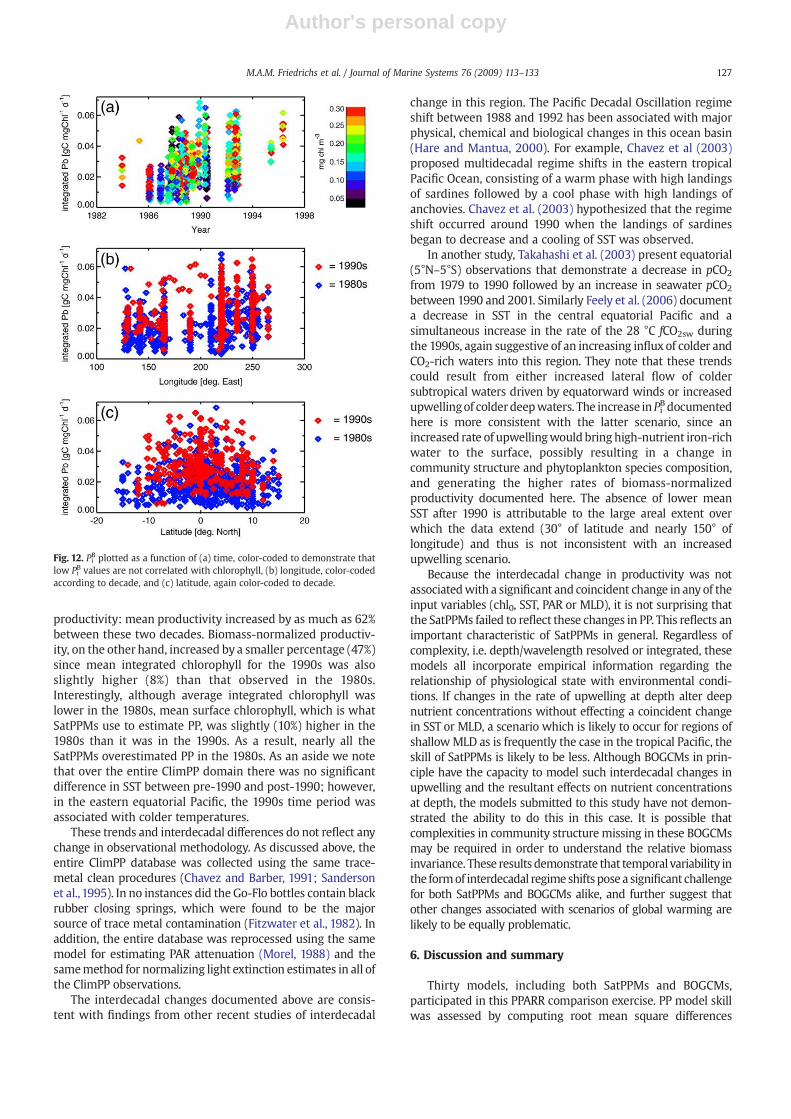
B is high; absolute misfit (|Δ|)typically is greatest for the lowest PiB values. Furthermore, theoldest data (from the early and mid-1980s) are generallycharacterized by relatively low Pi
B values (PiBb2.5 mmol C mgchl−1 d−1), whereas PiB measured from 1995 and 1996 exceed2.5 mmol C mg chl−1 d−1 (Fig. 12a). This change in Pi
B holdsover the entire ClimPP domain, not just the equatorial zone(Fig. 12b,c). Thus, the surprisingly high correlations betweenyear and misfit occur because: (1) all models, both theSatPPMs and the BOGCMs, perform poorly when Pi
B is low(b1 mmol C mg chl−1 d−1), and (2) 95% of these low Pi
B values
Fig. 10. As in Fig. 6, except RMSD is computed for the 1990s subset of the ClimPP data.
Fig. 9. As in Fig. 4, except statistics are computed for the 1990s subset of theClimPP data.
125M.A.M. Friedrichs et al. / Journal of Marine Systems 76 (2009) 113–133
Author's personal copy
occur in the 1980s (although there are more data pointspoleward of 10° in the 1980s than the 1990s (Fig. 12c), evenwhen only points between 10°N and 10°S are included, 95% ofthe Pi
Bb1 mmol C mg chl−1 d−1 values still occur in the 1980sportion of the ClimPP dataset). It is possible that the improved
performance of the models since 1990 is a reflection ofinherent problems associated with modeling low photo-synthesis rates for a given biomass.
The interdecadal variability in productivity per unitbiomass directly results from an increase in measured
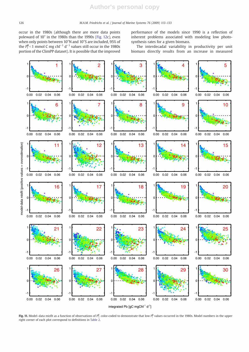
Fig. 11. Model–data misfit as a function of observations of PiB, color-coded to demonstrate that low PiB values occurred in the 1980s. Model numbers in the upper
right corner of each plot correspond to definitions in Table 2.
126 M.A.M. Friedrichs et al. / Journal of Marine Systems 76 (2009) 113–133
Author's personal copy
productivity: mean productivity increased by as much as 62%between these two decades. Biomass-normalized productiv-ity, on the other hand, increased by a smaller percentage (47%)since mean integrated chlorophyll for the 1990s was alsoslightly higher (8%) than that observed in the 1980s.Interestingly, although average integrated chlorophyll waslower in the 1980s, mean surface chlorophyll, which is whatSatPPMs use to estimate PP, was slightly (10%) higher in the1980s than it was in the 1990s. As a result, nearly all theSatPPMs overestimated PP in the 1980s. As an aside we notethat over the entire ClimPP domain there was no significantdifference in SST between pre-1990 and post-1990; however,in the eastern equatorial Pacific, the 1990s time period wasassociated with colder temperatures.
These trends and interdecadal differences do not reflect anychange in observational methodology. As discussed above, theentire ClimPP database was collected using the same trace-metal clean procedures (Chavez and Barber, 1991; Sandersonet al.,1995). In no instances did the Go-Flo bottles contain blackrubber closing springs, which were found to be the majorsource of trace metal contamination (Fitzwater et al., 1982). Inaddition, the entire database was reprocessed using the samemodel for estimating PAR attenuation (Morel, 1988) and thesamemethod for normalizing light extinction estimates in all ofthe ClimPP observations.
The interdecadal changes documented above are consis-tent with findings from other recent studies of interdecadal
change in this region. The Pacific Decadal Oscillation regimeshift between 1988 and 1992 has been associated with majorphysical, chemical and biological changes in this ocean basin(Hare and Mantua, 2000). For example, Chavez et al (2003)proposed multidecadal regime shifts in the eastern tropicalPacific Ocean, consisting of a warm phase with high landingsof sardines followed by a cool phase with high landings ofanchovies. Chavez et al. (2003) hypothesized that the regimeshift occurred around 1990 when the landings of sardinesbegan to decrease and a cooling of SST was observed.
In another study, Takahashi et al. (2003) present equatorial(5°N–5°S) observations that demonstrate a decrease in pCO2
from 1979 to 1990 followed by an increase in seawater pCO2
between 1990 and 2001. Similarly Feely et al. (2006) documenta decrease in SST in the central equatorial Pacific and asimultaneous increase in the rate of the 28 °C fCO2sw duringthe 1990s, again suggestive of an increasing influxof colder andCO2-rich waters into this region. They note that these trendscould result from either increased lateral flow of coldersubtropical waters driven by equatorward winds or increasedupwellingof colderdeepwaters. The increase inPi
B documentedhere is more consistent with the latter scenario, since anincreased rate of upwellingwould bring high-nutrient iron-richwater to the surface, possibly resulting in a change incommunity structure and phytoplankton species composition,and generating the higher rates of biomass-normalizedproductivity documented here. The absence of lower meanSST after 1990 is attributable to the large areal extent overwhich the data extend (30° of latitude and nearly 150° oflongitude) and thus is not inconsistent with an increasedupwelling scenario.
Because the interdecadal change in productivity was notassociatedwith a significant and coincident change in any of theinput variables (chl0, SST, PAR or MLD), it is not surprising thatthe SatPPMs failed to reflect these changes in PP. This reflects animportant characteristic of SatPPMs in general. Regardless ofcomplexity, i.e. depth/wavelength resolved or integrated, thesemodels all incorporate empirical information regarding therelationship of physiological state with environmental condi-tions. If changes in the rate of upwelling at depth alter deepnutrient concentrations without effecting a coincident changein SST or MLD, a scenario which is likely to occur for regions ofshallowMLD as is frequently the case in the tropical Pacific, theskill of SatPPMs is likely to be less. Although BOGCMs in prin-ciple have the capacity to model such interdecadal changes inupwelling and the resultant effects on nutrient concentrationsat depth, the models submitted to this study have not demon-strated the ability to do this in this case. It is possible thatcomplexities in community structure missing in these BOGCMsmay be required in order to understand the relative biomassinvariance. These results demonstrate that temporal variability inthe formof interdecadal regime shifts pose a significant challengefor both SatPPMs and BOGCMs alike, and further suggest thatother changes associated with scenarios of global warming arelikely to be equally problematic.
6. Discussion and summary
Thirty models, including both SatPPMs and BOGCMs,participated in this PPARR comparison exercise. PP model skillwas assessed by computing root mean square differences
Fig. 12. PiB plotted as a function of (a) time, color-coded to demonstrate thatlow Pi
B values are not correlated with chlorophyll, (b) longitude, color-codedaccording to decade, and (c) latitude, again color-coded to decade.
127M.A.M. Friedrichs et al. / Journal of Marine Systems 76 (2009) 113–133
Author's personal copy
(RMSD) and by using a variety of skill assessment tools todetermine how well each model reproduced log10PP from anextensive in situ tropical Pacific database (ClimPP). This regionof the ocean was chosen specifically because earlier PPmodeling efforts demonstrated that the tropical Pacific repre-sents a significant challenge for satellite-based PP models.
A primary result of this model intercomparison effort isthat although skill varied substantially among the participat-ing models, model skill was not associated with modelcomplexity or model type. Overall, there was little significantdifference in the performance of the three different classes ofSatPPMs represented here (based on depth and wavelengthresolution). Also, neither SatPPMs nor BOGCMs performedsignificantly better based on the full suite of skill assessmentmethodologies, revealing that using output from SatPPMs toevaluate BOGCM simulations of PP is not an adequate test ofBOGCM skill.
Most models substantially underestimated PP variability,often by more than a factor of two. Specifically many of themodels, including all 9 depth-resolved satellite-based models(though Model 18 to a much lesser degree), produced too fewlow PP values (b0.2 g Cm−2 d−1). PPmodel developers need tobe aware of this model shortcoming, and should note that animprovement in the ability of productivity models to estimatePP at low rates of productivity will have a significant impacton PP model skill in the tropical Pacific and other oligotrophicregions across the globe.
Whereas nearly all models underestimated PP variability,model performance differed substantially in terms of howwell the models reproduced the mean and median PP. Severalmodels overestimated the median productivity by a factor oftwo, others underestimated productivity by nearly a factor oftwo, and others presented almost no bias. Thus, the modelswith the greatest skill were generally those with the lowestbias. PPARR2 concluded that removing bias was an immediategoal to improve model performance. The present studyconfirms that several participatingmodels have accomplishedthis goal. Although, as noted above, in general there was littledifference in the performance of different classes of models,one exception is in terms of bias: the simplest models werecharacterized by significantly less bias than those thatresolved wavelength and depth.
In a best-case scenario, more than half of the total RMSDassociated with the SatPPMs could be attributed to uncertain-ties in input variables and the PP data. Whereas the skill ofcertain models could increase dramatically if the inputvariables were known more accurately (e.g. many of themodels that use the MLD fields), the skill of other models,including the simple square root of chlorophyll relationshipthat uses only the chl0 inputfield,wouldnot undergo the samelevel of improvement. In general, the subset of models basedon the Vertically Generalized Productivity Model (Behrenfeldand Falkowski,1997b) showa relatively small improvement inskill when uncertainties in input variables and PP data areconsidered, primarily because of their inherent insensitivity toPAR. On the contrary, the skills of PP models that utilize MLDin their computations of productivity are severely limited byuncertainties in MLD estimates, suggesting that furtherdevelopment of models that require MLD input fields is notadvised, especially since high quality MLD fields are notreadily available.
The specific models that demonstrate the greatest skill varydepending on which skill assessment methods are used. Forinstance, if total root mean square difference is used as thesingle criteria for skill, Model 18 (Mélin, 2003), which usesbiogeographical provinces to define the necessary modelparameters, performs best. Model 1, the simplistic sqrt(chl0)model, performs nearly as well according to this criterion,however this is partially due to the fact that models thatunderestimate variance result in lower total RMSD scores (Jolliffet al., 2009-this volume). Ten of the 30 models are associatedwith biases that are smaller than the levels of PPuncertaintyweassume here. One of the BOGCMs (Model 29: Tjiputra et al.,2007) produces the lowest bias, however one of the VGPMs(Model 12) and thedepth-resolvedModel 13 (Armstrong, 2006)also have negligible biases. In terms of reproducing theobserved PP variability, two depth and wavelength-resolvedmodels outperform the others (Model 16: Smyth et al., 2005and Model 18: Mélin, 2003). Model 18, as well as Model 27(Gregg, 2003) produce PP fields that are most highly correlatedwith thedata,whereasModel 29 (Tjiputra et al., 2007) producesPP fields that have nearly the same variance as the ClimPP data.Cumulative fractional distributions indicate that Model 11(Morel and Maritorena, 2001) produces PP distributions thatmost closely reproduce the observations. It is clearly notpossible to identify one single model that is most skilledaccording to all the criteria listed above, however, the specificmodels highlighted here are examples of models that performparticularly well in these analyses.
In order to better understand why certain models havegreater skill than others and what environmental conditionscontrol performance, correlations betweenmodel–data misfitand a number of relevant variables were computed. Surpris-ingly, model–data misfit was highly correlated to year foralmost all of the SatPPMs as well as for some of the BOGCMs.Both primary productivity and biomass-normalized produc-tivity in the ClimPP database were substantially higher in the1990s than in the 1980s. This interdecadal variability may beassociated with a change in upwelling rate within the tropicalPacific, a hypothesis that is consistent with previous studies(Takahashi et al., 2003; Chavez et al., 2003; Feely et al., 2006).The observed interdecadal change in integrated productivityper unit biomass within the ClimPP database was not asso-ciated with a coincident change in the surface expression ofchlorophyll, temperature, or PAR, probably because of thetypically shallow MLD in the tropical Pacific. As a result, theSatPPMs were unable to correctly estimate this interdecadalvariability in productivity. Although BOGCMs should theore-tically have the ability to replicate the increased upwelling ofnutrients and the effect of this on productivity, this study hasshown that this remains a challenge for the current genera-tion of BOGCMs. These results suggest that interdecadal andglobal changeswill be a significant challenge for both SatPPMsand BOGCMs alike.
The success of these types of comparison exercises isillustrated by the continual modification and improvement ofthe participating models and the resulting improvement inmodel skill. The previous PPARR2 exercise (Campbell et al.,2002) specifically highlighted bias as a major contributor tototal RMSD. As demonstrated here, bias has been effectivelyreduced in several participating models. PPARR2 used theJoint Global Ocean Flux Study equatorial Pacific process study
128 M.A.M. Friedrichs et al. / Journal of Marine Systems 76 (2009) 113–133
Author's personal copy
data collected on and off the equator at 140°W in 1992 tocompute the average total RMSD of log10PP for their twelveparticipating models. Using the identical dataset in ananalogous computation, the average total RMSD is computedfrom 20 of the SatPPMs participating in this exercise (Models2–21). The resulting RMSDs (on equator: 0.21; off equator:0.23) are 58% and 35% lower, respectively, then thosecomputed 6 years ago in PPARR2 (on equator: 0.50; offequator: 0.31). If this rate of model improvement continues,within a little more than a decade total RMSD can be expectedto fall to within the level of observational uncertainty (0.07).
Acknowledgements
This research was supported by a grant from the NationalAeronautics and Space Agency Ocean Biology and Biogeo-chemistry program (NNG06GA03G), as well as by numerousother grants to the various participating investigators. JasonJolliff, John Cullen and an anonymous reviewer providedmany useful comments, which improved the final version ofthe manuscript. The AVHRR Oceans Pathfinder SST data wereobtained from the Physical Oceanography Distributed ActiveArchive Center (PO.DAAC) at the NASA Jet PropulsionLaboratory, Pasadena, CA. Shortwave radiation data wereprovided by the NOAA-ESRL Physical Sciences Division,Boulder Colorado from their website at http://www.cdc.noaa.gov. We thank Raghu Murtugudde for providing themixed layer depths for the ClimPP database. We are alsograteful for the hard work of the many scientists who helpedacquire the ClimPP database. This is VIMS contribution #2904.
Appendix A
A.1. DI/WI SatPPMs
Model 1: This model estimates PP as:
PP g C m−2 d−1h i
¼ chl0 mg chl m−3� � 1=2(Eppley et al., 1985). It ignores any external forcing or
changes in physiological state. While other models incorpo-rate information regarding geography or forcing fields, thismodel assumes that the standing stock is sole determinant ofphotosynthetic rate. All biomass performs identically. Thissimplicity is inherently elegant because biomass is, for mostof the ocean, an excellent indicator of nutrient supply andpresence of light.
Model 2: This is a variant of the original Howard, Yoder,Ryan model (HYR, Howard and Yoder, 1997; Model 3) whichintegrates photosynthesis to the euphotic depth as defined inBehrenfeld and Falkowski (1997b) rather than to the MLD(Carr, 2002).
Model 3: This is the original HYR model, which for manyyears was a standard MODIS algorithm. Maximum growthrate is parameterized as a function of SST according to Eppley(1972). Primary productivity is integrated to the MLD ratherthan to the euphotic depth.
Model 4: This HYR variant uses MLD information toquantify the photoadaptive variables within the euphoticzone, as well as to address water column partitioning ofprimary productivity relative to euphotic depth.
Model 5: This model uses an artificial neural network toperform a generalized nonlinear regression of PP on severalpredictive variables, including latitude, longitude, day length,MLD, SST, Popt
B (computed according to Behrenfeld andFalkowski (1997b)), PAR, and chl0 (Scardi, 2000; Scardi, 2001).Since there are insufficient data to calibrate the neural networkthroughout the tropical Pacific, PP values from other models(VGPM, HYR, and theMOD-27 formulation (Esaias,1996)) wereconsidered measurements where there were none.
Model 6: This model is based on the formulation obtainedthrough dimensional analysis by Platt and Sathyendranath(1993). The photosynthetic parameter (Pmax
B ) is assigned bycombining a temperature-dependent relationship for themaximum growth rate (Eppley, 1972) with a variable carbonto chlorophyll ratio following the statistical relationship ofCloern et al. (1995). Primary production is integrated to the 1%light level.
Model 7: The Carbon-based Production Model (CbPM)represents a new approach to NPP assessment that utilizessatellite information on both surface chlorophyll and parti-culate backscatter (bbp) at 443 nm, which is converted intophytoplankton carbon biomass (C) (Behrenfeld et al., 2005).This expanded information set allows the ratio of chl:C to becalculated and related to phytoplankton growth rates (m),such that NPP is then calculated as the product of C andmu. Inthe current application of the CbPM, no field data wereprovided on bbp, so phytoplankton C was estimated using‘typical values’ derived from SeaWiFS data for a given samplelocation. This lack of coincident field bbp data compromisesthe performance of the CbPM in the current model-field datacomparison. Vertical structure in this version of the CbPM isas assumed in Model 8.
Model 8: The Vertically Generalized Production Model(VGPM) developed by Behrenfeld and Falkowski (1997b) isone of the most widely known and used WIDI PP models andis one of two standard MODIS algorithms. The maximumobserved photosynthetic rate within the water column, PoptB ,is obtained as a 7th-order polynomial of SST.
Model 9: This model only differs fromModel 8 in that PoptB isestimated as an exponential function of temperature followingEppley (1972).
Model 10: This VGPM variant formulates PoptB as a functionof SST and chl0 (Yamada et al., 2005; Kameda and Ishizaka,2005). The model is based on the assumptions that changes inchlorophyll concentration depend on the abundance of largephytoplankton and that chlorophyll-specific productivity isinversely proportional to phytoplankton size.
Model 11: This VGPM variant uses the continuous functionof Morel and Berthon (1989) to estimate total integratedchlorophyll, which in turn is used to estimate the euphoticdepth with the equations proposed by Morel and Maritorena(2001).
Model 12: This VGPM variant differs from Model 8 in thatPoptB (mg C mg chl−1 h−1) is estimated as a function of chl0 (mg
chl m−3) only. This empirical relationship was derived fromEqPac data (PoptB =24×chl0+1).
A.2. DR/WI SatPPMs
Model 13: Photosynthesis per unit chlorophyll was deter-mined using an optimality-based model of nitrogen allocation
129M.A.M. Friedrichs et al. / Journal of Marine Systems 76 (2009) 113–133
Author's personal copy
and photoacclimation (Armstrong, 2006), which is in turnbased on the model of Geider et al. (1998). Photoacclimationand nitrogen allocation are determined as a function of lightand temperature; therefore both PAR and SST are used in theproductivity algorithm. Maximum photosynthetic rates weretaken to be an average ofmaximumNPP and GPP estimated forT. weissflogii in Armstrong (2006), and were assumed to haveEppley temperature dependence. Through the photoadaptationalgorithm, chlorophyll reflects nitrogen status, so that noadditional assumptions about nutrient limitation are needed.Chlorophyll concentration was assumed constant over thephotic zone and equal to surface chlorophyll, so that lightdecreases exponentially with depth. Photic zone depth (1%light) was determined from chlorophyll concentration andassumed extinction coefficients. The photic zone was assumedtobewell-mixed and cellswere assumed tobephotoacclimatedto average (10%) light. Column productivity is the integral overthe photic zone of (photosynthesis/chlorophyll)⁎chlorophyll.
Model 14: In this model the depth distribution of PAR isdetermined by chl0 while the depth distribution of chlor-ophyll is given by the PAR profile and chl0. Total productivityis empirically estimated as a function of surface temperatureand depth-dependent PAR and chlorophyll (Asanuma, 2006).
Model 15: This model is based on chlorophyll-specificphytoplankton absorption, which is parameterized empiri-cally as a function of SST (Marra et al., 2003). Absorption byphotosynthetic pigments is distinguished from total absorp-tion; the former is used to calculate productivity and the latteris used to estimate light attenuation in the water column. Therate of photosynthesis is quantum yield times absorbedirradiance, obtained from a hyperbolic tangent and a constantmaximum quantum yield, ϕmax. The depth profile of chlor-ophyll is estimated assuming a Gaussian shape with para-meters determined by the surface value. The attenuationcoefficient of chlorophyll is also SST-dependent.
A.3. DR/WR SatPPMs
Model 16: This model is an implementation of the Morel(1991) model in which the depth distribution of chlorophyll isassumed constant throughout the water column. The broad-band incident PAR is spectrally resolved using a lookup tablegenerated from a single run of the Gregg and Carder (1990)marine irradiance model where the effects of clouds andaerosols are essentially linearly scaled. The model uses 60-mintime and 10-m depth steps at 5-nm wavelength resolutionwhen run using the global datasets (Smyth et al., 2005).
Model 17: This model is the lookup table described inSmyth et al. (2005) which uses a radiative transfermodel withparameterizations for Colored Dissolved Organic Matter(CDOM). The model is based on Morel (1991) with incidentirradiance parameterized in the same manner as Model 16.
Model 18: This model follows that of Platt and Sathyen-dranath (1988) as implemented at global scale by Longhurstet al. (1995). It uses biogeographical provinces to define thevalues of the parameters to describe the light–photosynthesiscurve and the chlorophyll depth profile. Photosyntheticparameters were updated using an extended dataset providedby the Bedford Institute of Oceanography and an extensiveliterature review. Spectral surface irradiance is first estimatedindependently with the model of Gregg and Carder (1990)
combinedwith a correction for cloud cover and then scaled tomatch the PAR values provided for the exercise. Spectral lightis subsequently propagated in the water column with a bio-optical model with updated parameterizations of the inherentoptical properties. All changes to the original implementationof Longhurst et al. (1995) are detailed by Mélin (2003).
Model 19: This model derives spectral irradiance from PARusing Tanre et al. (1990), and assumes a vertically uniformchlorophyll profile. Quantum yield is parameterized as amaximum value times both a light dependent term (Waterset al., 1994; Bidigare et al., 1992) and a temperature-dependentterm. Temperature dependence was assumed to be sigmoidal,andwas based on a vertical profile of temperature derived fromSST and MLD.
Model 20: This is a spectral light–photosynthesis modelpublished by Morel (1991). It is formulated using chlorophyll-specific wavelength-resolved absorption and quantum yield.Temperature dependence is given by the parameterizationof Pmax
B , which follows Eppley (1972). The chlorophyll profileis determined to be well-mixed or stratified accordingto the ratio of MLD and the euphotic depth, and if stratified,assigned a Gaussian profile as in Morel and Berthon (1989).Mean photo-physiological parameters are from Morel etal. (1996). The model is run in its ‘satellite’ version AntoineandMorel (1996), where PP is the product of integral biomass,the daily irradiance, and Ψ⁎ (the cross-section of algaefor photosynthesis per unit of areal chlorophyll biomass).Lookup tables for Ψ⁎ were previously generated using thefull DR/WR model, and are used to increase computationalefficiency.
Model 21: This model represents an expansion in both thephysiological attributes of the original CbPM (Model 7) and thespace- and time-resolution of the model, and is described indetail in Westberry et al. (2008). The model requires surfacechlorophyll concentration data and particulate backscattercoefficients (bbp) at 443 nm. As with Model #7, execution ofModel #21 for the current study required the estimation of bbpfrom the SeaWiFS record, as no coincident field data for bbpwere available. Vertical structure in chlorophyll concentrationin thismodel is drivenprimarily by photoacclimation of cellularchlorophyll, with additional adjustments made for changes innutrient stress through the water column.
A.4. BOGCMs
Model 22: This BOGCM (Christian et al., 2002) uses a 20-layer reduced-gravity σ-coordinate model, with the first layercorresponding to the ocean's mixed layer. The grid employedhere stretches from 124°E to 76°W with uniform 1° resolutionin longitude, and from 30°S to 30°N with maximal latitudinalresolution in the equatorial band (1/3° at latitudes b10°). Themodel was run using NCEP weekly (6 day) mean wind stressand monthly interannual precipitation. The nitrogen and ironbased ecosystem model has two size classes each of phyto-plankton, zooplankton, and detritus, and the nutrients nitrate,ammonium, and iron. Phytoplankton growth is simultaneouslylimited by irradiance as well as nitrogen and iron availability,with fixed Fe/N ratios so that iron in all compartments exceptthe dissolved pool is not modelled explicitly.
Model 23: This BOGCM is amodification ofModel 22 (Wanget al., 2005, 2006) and differs primarily by having a saturating
130 M.A.M. Friedrichs et al. / Journal of Marine Systems 76 (2009) 113–133
Author's personal copy
(Ivlev) rather than a nonsaturating (multiplicative) grazerfunctional response. In addition it utilizes an additionalquadratic mortality term that confers stability and suppressesoscillatory solutions in the case of saturable grazing (Wanget al., 2005). Additionalminormodifications fromthepublishedversions are discussed in Christian et al. (in press).
Model 24: The Biogeochemical Elemental Cycling (BEC)ocean model simulates the biogeochemical cycling of carbon,oxygen, nitrate, phosphate, iron, silicate, and alkalinity. Theecosystem has multiple, potentially growth limiting nutrients(nitrogen, phosphorus, silicon, and iron) and four phytoplank-ton groups (diatoms, diazotrophs, coccolithophores, and pico-phytoplankton) (Moore et al., 2002, 2004; Doney et al., 2009-this issue). Growth rates can be limited by available nutrientsand/or light levels. Full carbonate chemistry, as well as sinkingparticulate and semi-labile dissolved organic pools are includedin a global, 3D context without nutrient restoring (Moore et al.,2004). The BEC runs within the coarse resolution oceancomponent of the Community Climate System Model (Yeageret al., 2006), driven with time-varying atmospheric forcingfrom NCEP reanalysis and satellite data products (Doney et al.,2007).
Model 25: This prognostic ocean biogeochemistry/ecologymodel considers 25 tracers including three phytoplanktongroups, two forms of dissolved organic matter, heterotrophicbiomass, and dissolved inorganic species for coupled C, N, P, Si,Fe, CaCO3, O2 and lithogenic cycling with flexible N:P:Festoichiometry. The model includes such processes as gasexchange, atmospheric deposition, scavenging, N2 fixationand denitrification. Loss of phytoplankton is parameterizedthrough the size-based relationship of Dunne et al. (2005),river inputs, and sediment processes. This biogeochemistrywas run in the Modular Ocean Model version 4 (Griffies et al.,2005) with 50 vertical z-coordinate layers and a nominally 1°global resolution horizontal B-grid with tri-polar coordinatesto resolve the arctic and finer detail of 1/3° near the equator.The model was forced with 6-hourly and interannuallyvarying forcing from the atmospheric reanalysis of Large andYeager (2004).
Model 26: The NASA Ocean Biogeochemical Model(NOBM) simulates four phytoplankton groups (diatoms,chlorophytes, cyanobacteria, and coccolithophores) and fournutrients (nitrate, ammonium, silica, and iron) (Gregg andCasey, 2007). The model is approximately 0.8° resolutionwith14 vertical layers in quasi-isopycnal configuration. The modelwas forced by monthly mean winds and shortwave radiationfrom NCEP for 1979–2004.
Model 27: In this NOBM variant (Gregg, 2008), NODC datafor 1979–2004 were assimilated using the ConditionalRelaxation Analysis Method. The assimilation affected themodel representations of total chlorophyll (sum of the 4phytoplankton groups), but not the individual communitydistributions directly. Primary production was affected by thechange in total chlorophyll, as well as by indirect effects suchas subsurface irradiance resulting from absorption andscattering by the changed chlorophyll field.
Model 28: The PISCES-T model is a two phytoplankton,two zooplankton, three detritus, three nutrient DynamicGreen Ocean Model. It has variable Fe:C, Chl:C and Si:C ratiosand fixed N:C:O. It is embedded in the OPA8 OGCM, initializedwith observations, and forced by daily NCEP reanalysis
(Buitenhuis et al., 2006). No nutrient restoring was used.The model was run from 1948 to 2006 (Le Quere et al., 2007).
Model 29: The Hamburg Ocean Carbon Cycle (HAMOCC5)model uses monthly climatology forcing with approximately3.5°×3.5° horizontal degree resolution and 22 vertical layerswith thickness varying from 50 m at the surface to 700 m inthe deepest layer (Maier-Reimer, 1993). The model employsan NPZD-type ecosystem model with two phytoplanktonfunctional groups (diatoms and calcifiers) withmulti-nutrient(nitrate, phosphate, silicate and iron) limitation. Productivityis simulated with a 3-day time step (Six and Maier-Reimer,1996; Howard et al., 2006).
Model 30: The physical model is based on the RegionalOcean Modeling System (ROMS), which has been configuredfor the Pacific Ocean at 50-km horizontal resolution and 20vertical layers (Wang and Chao, 2004). The biogeochemicalmodel is based on the Carbon, Silicate, Nitrogen Ecosystem(CoSINE) model developed by Chai et al. (2002, 2003). TheCoSINE model includes silicate, nitrate and ammonium, twophytoplankton groups, two zooplankton grazers, and twodetrital pools. The model is initialized with climatological,temperature, salinity, nutrients and TCO2. When forced withdaily air–sea fluxes (wind stress, heat flux, and freshwaterexchange) derived from NCEP/NCAR reanalysis (Kalnay et al.,1996) for the period of 1984 to 2005, the Pacific ROMS-CoSINEmodel is able to realistically reproduce the evolution of ENSOevents (1992–93; 1997–98) as well as a sharp change of thecirculation and thermal structure for the Pacific Ocean in1998–99 (Liu and Chai, 2008).
Appendix B. Supplementary data
Supplementarydata associatedwith this article canbe found,in the online version, at doi:10.1016/j.jmarsys.2008.05.010.
References
Antoine, D., Morel, A., 1996. Oceanic primary production: I. Adaptation of aspectral light–photosynthesis model in view of application to satellitechlorophyll observations. Global Biogeochemical Cycles 10, 43–55.
Armstrong, R.A., 2006. Optimality-based modeling of nitrogen allocation andphoto acclimation in photosynthesis. Deep-Sea Research II 53, 513–531.
Asanuma, I., 2006. Depth and time resolved primary productivity modelexamined for optical properties of water, global climate change andresponse of carbon cycle in the equatorial Pacific and Indian Oceans andadjacent landmasses. Elsevier Oceanography Series 73, 89–106 pp.
Barber, R.T., Borden, L., Johnson, Z., Marra, J., Knudson, C., Trees, C., 1997.Ground truthing modeled kPAR and on deck primary productivityincubations with in situ observations. Ocean Optics XIII 2963, 834–839.
Barber, R.T., Chavez, F.P., 1991. Regulation of primary productivity rate in theequatorial Pacific Ocean. Limnology and Oceanography 36, 1803–1815.
Barber, R.T., Marra, J., Bidigare, R.C., Codispoti, L.A., Halpern, D., Johnson, Z., Latasa,M.,Goericke,R., Smith, S.L., 2001. Primaryproductivityand its regulation in theArabian Sea during 1995. Deep-Sea Research II 48, 1127–1172.
Barber, R.T., Sanderson, M.P., Lindley, S.T., Chai, F., Newton, J., Trees, C.C., Foley,D.G., Chavez, F.P., 1996. Primary productivity and its regulation in theequatorial Pacific during and following the 1991–1992 El Nino. Deep SeaResearch I 43, 933–969.
Behrenfeld, M.J., Falkowski, P.G., 1997a. A consumer's guide to phytoplanktonprimary productivity models. Limnology and Oceanography 42, 1479–1491.
Behrenfeld, M.J., Falkowski, P.G., 1997b. Photosynthetic rates derived fromsatellite-based chlorophyll concentration. Limnology and Oceanography42, 1–20.
Behrenfeld, M.J., Boss, E., Siegel, D.A., Shea, D.M., 2005. Carbon-based oceanproductivity and phytoplankton physiology from space. Global Biogeo-chemical Cycles 19, GB1006. doi:10.1029/2004GB002299.
Behrenfeld, M.J., O, ' Malley, R.T., Siegel, D.A., McClain, C.R., Sarmiento, J.L.,Feldman, G.C., Milligan, A.J., Falkowski, P.G., Letelier, R.M., Boss, E.S., 2006.
131M.A.M. Friedrichs et al. / Journal of Marine Systems 76 (2009) 113–133
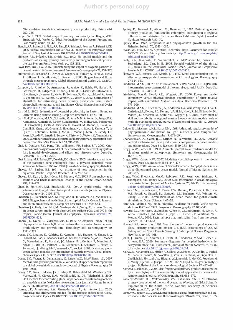
Author's personal copy
Climate-driven trends in contemporary ocean productivity. Nature 444,752–755.
Berger, W.H., 1989. Global maps of primary productivity. In: Berger, W.H.,Smetacek, V.S., Wefer, G. (Eds.), Productivity of the Ocean: Present andPast. Wiley, Berlin, pp. 429–455.
Bianchi, A.A., Bianucci, L., Piola, A.R., Pino, D.R., Schloss, I., Poisson, A., Balestrini, C.F.,2005. Vertical stratification and air–sea CO2 fluxes in the Patagonian shelf.Journal of Geophysical Research 110, C07003. doi:10.1029/2004JC002488.
Bidigare, R.R., Prézelin, B.B., Smith, R.C., 1992. Bio-optical models and theproblems of scaling, primary productivity and biogeochemical cycles inthe sea. Plenum Press, New York, pp. 175–212.
Boyd, P.W., Trull, T.W., 2007. Understanding the export of biogenic particles inoceanicwaters: is there consensus? Progress inOceanography 72, 276–312.
Buitenhuis, E., Le Quéré, C., Olivier, A., Grégory, B., Bunker, A., Hirst, A., Ikeda,T., O'Brien, T., Piontkovski, S., Straile, D., 2006. Biogeochemical fluxesthrough mesozooplankton. Global Biogeochemical Cycles 20, GB2003.doi:10.1029/2005GB002511.
Campbell, J., Antoine, D., Armstrong, R., Arrigo, K., Balch, W., Barber, R.,Behrenfeld, M., Bidigare, R., Bishop, J., Carr, M.-E., Esaias, W., Falkowski, P.,Hoepffner, N., Iverson, R., Kiefer, D., Lohrenz, S., Marra, J., Morel, A., Ryan,J., Vedernikov, V., Waters, K., Yentsch, C., Yoder, J., 2002. Comparison ofalgorithms for estimating ocean primary production from surfacechlorophyll, temperature, and irradiance. Global Biogeochemical Cycles16. doi:10.1029/2001GB001444.
Carr, M.E., 2002. Estimation of potential productivity in Eastern BoundaryCurrents using remote sensing. Deep-Sea Research II 49, 59–80.
Carr, M.-E., Friedrichs, M.A.M., Schmeltz, M., Aita, M.N., Antoine, D., Arrigo, K.R.,Asanuma, I., Aumont, O., Barber, R., Behrenfeld, M., Bidigare, R., Buitenhuis,E.T., Campbell, J., Ciotti, A., Dierssen, H., Dowell, M., Dunne, J., Esaias, W.,Gentili, B., Gregg, W., Groom, S., Hoepffner, N., Ishizaka, J., Kameda, T., LeQuéré, C., Lohrenz, S., Marra, J., Mélin, F., Moore, J., Morel, A., Reddy, T.E.,Ryan, J., Scardi,M., Smyth, T., Turpie, K., Tilstone,G.,Waters, K., Yamanaka, Y.,2006. A comparison of global estimates ofmarine primary production fromocean color. Deep-Sea Research II 53, 741–770.
Chai, F., Dugdale, R.C., Peng, T.H., Wilkerson, F.P., Barber, R.T., 2002. One-dimensional ecosystemmodel of the equatorial Pacific upwelling system.Part I: model development and silicon and nitrogen cycle. Deep-SeaResearch II 49, 2713–2745.
Chai, F., Jiang,M.S., Barber, R.T., Dugdale, R.C., Chao,Y., 2003. Interdecadalvariationof the transition zone chlorophyll front: a physical–biological modelsimulation between 1960 and 1990. Journal of Oceanography 59, 461–475.
Chavez, F.P., Barber, R.T., 1991. An estimate of new production in theequatorial Pacific. Deep-Sea Research 34, 1229–1243.
Chavez, F.P., Ryan, J., Lluch-Cota, S.E., Ñiquen, M.C., 2003. From anchovies tosardines and back: mulitdecadal change in the Pacific Ocean. Science299, 217–221.
Chen, D., Rothstein, L.M., Busalacchi, A.J., 1994. A hybrid vertical mixingscheme and its application to tropical ocean models. Journal of PhysicalOceanography 24, 2156–2179.
Christian, J.R., Verschell, M.A., Murtugudde, R., Busalacchi, A.J., McClain, C.R.,2002. Biogeochemical modelling of the tropical Pacific Ocean. I: Seasonaland interannual variability. Deep-Sea Research II 49, 509–543.
Christian, J.R., Feely, R.A., Ishii, M., Murtugudde, R., Wang, X., in press. Testingan ocean carbon model with observed sea surface pCO2 and DIC in thetropical Pacific Ocean. Journal of Geophysical Research. doi:10.1029/2007JC004428.
Cloern, J.E., Grenz, C., VidergarLucas, L., 1995. An empirical model of thephytoplankton chlorophyll:carbon ratio— the conversion factor betweenproductivity and growth rate. Limnology and Oceanography 40,1313–1321.
Doney, S.C., Lindsay, K., Caldeira, K., Campin, J.-M., Drange, H., Dutay, J.-C.,Follows, M., Gao, Y., Gnanadesikan, A., Gruber, N., Ishida, A., Joos, F., Madec,G., Maier-Reimer, E., Marshall, J.C., Matear, R.J., Monfray, P., Mouchet, A.,Najjar, R., Orr, J.C., Plattner, G.-K., Sarmiento, J., Schlitzer, R., Slater, R.,Totterdell, I.J., Weirig, M.-F., Yamanaka, Y., Yool, A., 2004. Evaluating globalocean carbon models: the importance of realistic physics. Global Biogeo-chemical Cycles 18, GB3017. doi:10.1029/2003GB002150.
Doney, S.C., Yeager, S., Danabasoglu, G., Large, W.G., McWilliams, J.C., 2007.Mechanisms governing interannual variability of upper-ocean temperaturein a global ocean hindcast simulation. Journal of Physical Oceanography 37,1918–1938.
Doney, S.C., Lima, I., Moore, J.K., Lindsay, K., Behrenfeld, M., Westberry, T.K.,Mahowald, N., Glover, D.M., McGillicuddy Jr., D.J., Takahashi, T., 2009.Skill metrics for confronting global upper ocean ecosystem-biogeochem-istrymodels againstfield andremote sensingdata. Journal ofMarine Systems76, 95–112 (this issue). doi:10.1016/j.jmarsys.2008.05.015.
Dunne, J.P., Armstrong, R.A., Gnanadesikan, A., Sarmiento, J.L., 2005.Empirical and mechanistic models for the particle export ratio. GlobalBiogeochemical Cycles 19, GB02390. doi:10.1029/2004GB002390.
Eppley, R., Steward, E., Abbott, M., Heyman, U., 1985. Estimating oceanprimary production from satellite chlorophyll: introduction to regionaldifferences and statistics for the southern California Bight. Journal ofPlankton Research 7, 57–70.
Eppley, R.W., 1972. Temperature and phytoplankton growth in the sea.Fisheries Bulletin 70, 1063–1085.
Esaias, W., 1996. MODIS Algorithm Theoretical Basis Document for ProductMOD-27: Ocean Primary Productivity. http://modis.gsfc.nasa.gov/data/atbd/atbd-mod24.pdf.
Feely, R.A., Takahashi, T., Wanninkhof, R., McPhaden, M., Cosca, C.E.,Sutherland, S.C., Carr, M.-E., 2006. Decadal variability of the air–seaCO2 fluxes in the equatorial Pacific Ocean. Journal of GeophysicalResearch 111, C08S90. doi:10.1029/2005JC003129.
Fitzwater, W.E., Knauer, G.A., Martin, J.H., 1982. Metal contamination and itseffect on primary production measurement. Limnology and Oceanography27, 544–551.
Friedrichs, M.A.M., 2002. The assimilation of SeaWiFS and JGOFS EqPac datainto amarine ecosystemmodel of the central equatorial Pacific. Deep-SeaResearch II 49, 289–319.
Friedrichs, M.A.M., Hood, R.R., Wiggert, J.D., 2006. Ecosystem modelcomplexity versus physical forcing: quantification of their relativeimpact with assimilated Arabian Sea data. Deep-Sea Research II 53,576–600.
Friedrichs, M.A.M., Dusenberry, J.A., Anderson, L.A., Armstrong, R.A., Chai, F.,Christian, J.R., Doney, S.C., Dunne, J., Fujii, M., Hood, R., McGillicuddy, D.J.,Moore, J.K., Schartau, M., Spitz, Y.H., Wiggert, J.D., 2007. Assessment ofskill and portability in regional marine biogeochemical models: role ofmultiple planktonic groups. Journal of Geophysical Research 112, C08001.doi:10.1029/2006JC003852.
Geider, R.J., MacIntyre, H.L., Kana, T.M., 1998. A dynamic regulatory model ofphytoplanktonic acclimation to light, nutrients, and temperature.Limnology and Oceanography 43, 679–694.
Gnanadesikan, A., Slater, R.D., Gruber, N., Sarmiento, J.L., 2002. Oceanicvertical exchange and new production: a comparison between modelsand observations. Deep-Sea Research II 49, 363–401.
Gregg, W.W., Carder, K.L., 1990. A simple spectral solar irradiance model forcloudless maritime atmospheres. Limnology and Oceanography 35,1657–1675.
Gregg, W.W., Casey, N.W., 2007. Modeling coccolithophores in the globaloceans. Deep-Sea Research II 54, 447–477.
Gregg, W.W., 2008. Assimilation of SeaWiFS ocean chlorophyll data into athree-dimensional global ocean model. Journal of Marine Systems 69,205–255.
Gregg, W.W., Friedrichs, MA.M., Robinson, A.R., Rose, K.A., Schlitzer, R.,Thompson, K.R., Doney, S.C., 2009. Skill assessment in ocean biologicaldata assimilation. Journal of Marine Systems 76, 16–33 (this volume).doi:10.1016/j.jmarsys.2008.05.006.
Griffies, S.M., Gnanadesikan, A., Dixon, K.W., Dunne, J.P., Gerdes, R., Harrison,M.J., Rosati, A., Russell, J.L., Samuels, B.L., Spelman, M.J., Winton, M.,Zhang, R., 2005. Formulation of an ocean model for global climatesimulations. Ocean Science 1, 45–79.
Hare, S.R., Mantua, N.J., 2000. Empirical evidence for North Pacific regimeshifts in 1977 and 1989. Progress in Oceanography 47, 103–145.
Howard, E.C., Henriksen, J.R., Buchan, A., Reisch, C.R., Bürgmann, H., Welsh, R.,Ye, W., González, J.M., Mace, K., Joye, S.B., Kiene, R.P., Whitman, W.B.,Moran, M.A., 2006. Bacterial taxa that limit sulfur flux from the ocean.Science 314, 649–652.
Howard, K.L., Yoder, J.A., 1997. Contribution of the sub-tropical oceans toglobal primary production. In: Liu, C.-T. (Ed.), Proceedings of COSPARColloquium on Space Remote Sensing of Subtropical Oceans. Pergamon,New York, pp. 157–168.
Jolliff, J., Kindle, J.C., Shulman, I., Penta, B., Friedrichs, M.A.M., Helber, R.,Arnone, R.A., 2009. Summary diagrams for coupled hydrodynamic-ecosystem model skill assessment. Journal of Marine Systems 76, 64–82(this volume). doi:10.1016/j.jmarsys.2008.05.014.
Kalnay, E., Kanamitsu, M., Kistler, R., Collins, W., Deaven, D., Gandin, L., Iredell,M., Saha, S., White, G., Woollen, J., Zhu, Y., Leetmaa, A., Reynolds, B.,Chelliah, M., Ebisuzaki, W., Higgins, W., Janowiak, J., Mo, K.C., Ropelewski,C., Wang, J., Jenne, R., Joseph, D., 1996. The NCEP/NCAR 40-year reanalysisproject. Bulletin of the American Meteorological Society 77, 437–471.
Kameda, T., Ishizaka, J., 2005. Size-fractionated primary production estimatedby a two-phytoplankton community model applicable to ocean colorremote sensing. Journal of Oceanography 61, 663–672.
Koblentz-Mishke, O.I., Volknovinsky, V.V., Kabanova, Y.G., 1970. Planktonprimary production of the world ocean. In: Wooster, W. (Ed.), ScientificExploration of the South Pacific. National Academy of Sciences,Washington, D.C., pp. 183–193.
Large,W.G., Yeager, S.G., 2004.Diurnal todecadal global forcing foroceanand sea-ice models: the data sets and flux climatologies. TN-460+STR, NCAR, p. 105.
132 M.A.M. Friedrichs et al. / Journal of Marine Systems 76 (2009) 113–133
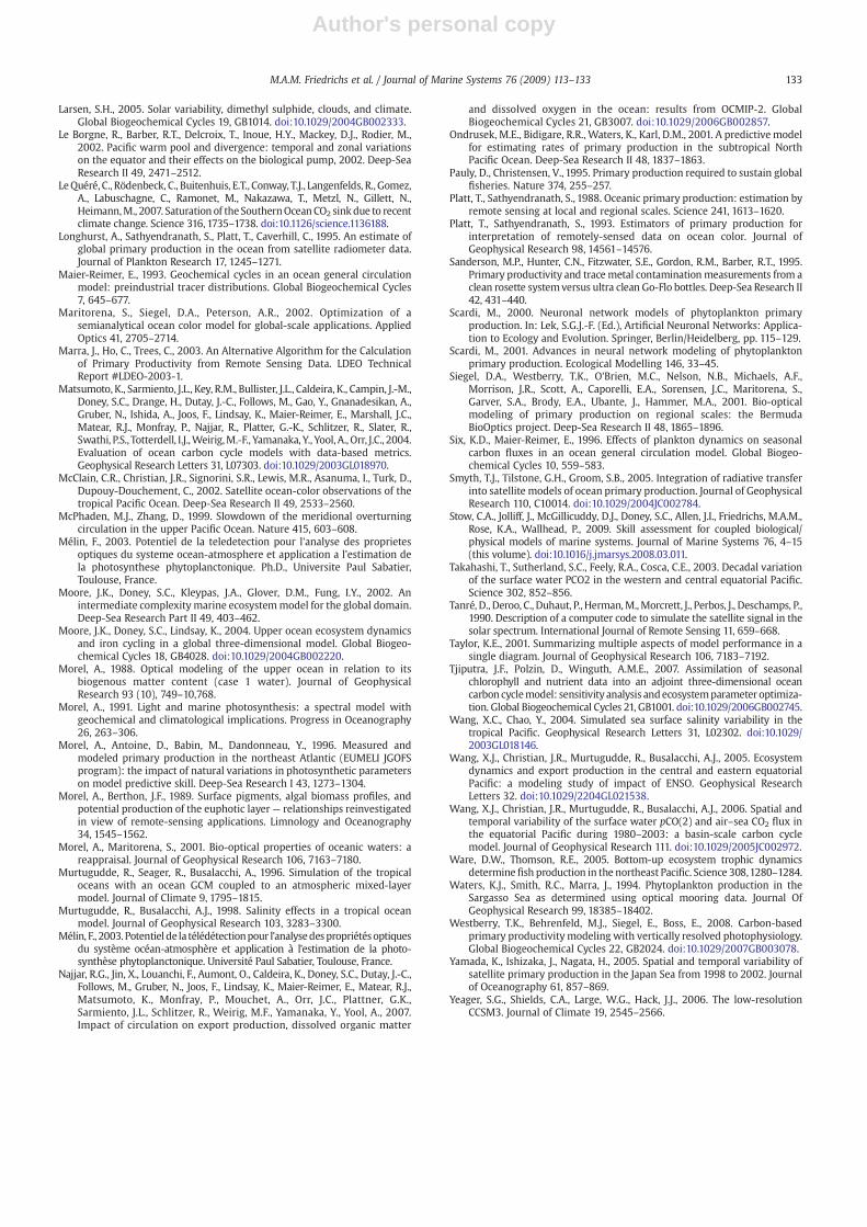
Author's personal copy
Larsen, S.H., 2005. Solar variability, dimethyl sulphide, clouds, and climate.Global Biogeochemical Cycles 19, GB1014. doi:10.1029/2004GB002333.
Le Borgne, R., Barber, R.T., Delcroix, T., Inoue, H.Y., Mackey, D.J., Rodier, M.,2002. Pacific warm pool and divergence: temporal and zonal variationson the equator and their effects on the biological pump, 2002. Deep-SeaResearch II 49, 2471–2512.
LeQuéré, C., Rödenbeck, C., Buitenhuis, E.T., Conway, T.J., Langenfelds, R., Gomez,A., Labuschagne, C., Ramonet, M., Nakazawa, T., Metzl, N., Gillett, N.,Heimann,M., 2007. Saturation of the SouthernOceanCO2 sink due to recentclimate change. Science 316, 1735–1738. doi:10.1126/science.1136188.
Longhurst, A., Sathyendranath, S., Platt, T., Caverhill, C., 1995. An estimate ofglobal primary production in the ocean from satellite radiometer data.Journal of Plankton Research 17, 1245–1271.
Maier-Reimer, E., 1993. Geochemical cycles in an ocean general circulationmodel: preindustrial tracer distributions. Global Biogeochemical Cycles7, 645–677.
Maritorena, S., Siegel, D.A., Peterson, A.R., 2002. Optimization of asemianalytical ocean color model for global-scale applications. AppliedOptics 41, 2705–2714.
Marra, J., Ho, C., Trees, C., 2003. An Alternative Algorithm for the Calculationof Primary Productivity from Remote Sensing Data. LDEO TechnicalReport #LDEO-2003-1.
Matsumoto, K., Sarmiento, J.L., Key, R.M., Bullister, J.L., Caldeira, K., Campin, J.-M.,Doney, S.C., Drange, H., Dutay, J.-C., Follows, M., Gao, Y., Gnanadesikan, A.,Gruber, N., Ishida, A., Joos, F., Lindsay, K., Maier-Reimer, E., Marshall, J.C.,Matear, R.J., Monfray, P., Najjar, R., Platter, G.-K., Schlitzer, R., Slater, R.,Swathi, P.S., Totterdell, I.J.,Weirig,M.-F., Yamanaka, Y., Yool, A., Orr, J.C., 2004.Evaluation of ocean carbon cycle models with data-based metrics.Geophysical Research Letters 31, L07303. doi:10.1029/2003GL018970.
McClain, C.R., Christian, J.R., Signorini, S.R., Lewis, M.R., Asanuma, I., Turk, D.,Dupouy-Douchement, C., 2002. Satellite ocean-color observations of thetropical Pacific Ocean. Deep-Sea Research II 49, 2533–2560.
McPhaden, M.J., Zhang, D., 1999. Slowdown of the meridional overturningcirculation in the upper Pacific Ocean. Nature 415, 603–608.
Mélin, F., 2003. Potentiel de la teledetection pour l'analyse des proprietesoptiques du systeme ocean-atmosphere et application a l'estimation dela photosynthese phytoplanctonique. Ph.D., Universite Paul Sabatier,Toulouse, France.
Moore, J.K., Doney, S.C., Kleypas, J.A., Glover, D.M., Fung, I.Y., 2002. Anintermediate complexity marine ecosystemmodel for the global domain.Deep-Sea Research Part II 49, 403–462.
Moore, J.K., Doney, S.C., Lindsay, K., 2004. Upper ocean ecosystem dynamicsand iron cycling in a global three-dimensional model. Global Biogeo-chemical Cycles 18, GB4028. doi:10.1029/2004GB002220.
Morel, A., 1988. Optical modeling of the upper ocean in relation to itsbiogenous matter content (case 1 water). Journal of GeophysicalResearch 93 (10), 749–10,768.
Morel, A., 1991. Light and marine photosynthesis: a spectral model withgeochemical and climatological implications. Progress in Oceanography26, 263–306.
Morel, A., Antoine, D., Babin, M., Dandonneau, Y., 1996. Measured andmodeled primary production in the northeast Atlantic (EUMELI JGOFSprogram): the impact of natural variations in photosynthetic parameterson model predictive skill. Deep-Sea Research I 43, 1273–1304.
Morel, A., Berthon, J.F., 1989. Surface pigments, algal biomass profiles, andpotential production of the euphotic layer— relationships reinvestigatedin view of remote-sensing applications. Limnology and Oceanography34, 1545–1562.
Morel, A., Maritorena, S., 2001. Bio-optical properties of oceanic waters: areappraisal. Journal of Geophysical Research 106, 7163–7180.
Murtugudde, R., Seager, R., Busalacchi, A., 1996. Simulation of the tropicaloceans with an ocean GCM coupled to an atmospheric mixed-layermodel. Journal of Climate 9, 1795–1815.
Murtugudde, R., Busalacchi, A.J., 1998. Salinity effects in a tropical oceanmodel. Journal of Geophysical Research 103, 3283–3300.
Mélin, F., 2003. Potentiel de la télédétectionpour ľanalysedespropriétésoptiquesdu système océan-atmosphère et application à ľestimation de la photo-synthèse phytoplanctonique. Université Paul Sabatier, Toulouse, France.
Najjar, R.G., Jin, X., Louanchi, F., Aumont, O., Caldeira, K., Doney, S.C., Dutay, J.-C.,Follows, M., Gruber, N., Joos, F., Lindsay, K., Maier-Reimer, E., Matear, R.J.,Matsumoto, K., Monfray, P., Mouchet, A., Orr, J.C., Plattner, G.K.,Sarmiento, J.L., Schlitzer, R., Weirig, M.F., Yamanaka, Y., Yool, A., 2007.Impact of circulation on export production, dissolved organic matter
and dissolved oxygen in the ocean: results from OCMIP-2. GlobalBiogeochemical Cycles 21, GB3007. doi:10.1029/2006GB002857.
Ondrusek, M.E., Bidigare, R.R., Waters, K., Karl, D.M., 2001. A predictive modelfor estimating rates of primary production in the subtropical NorthPacific Ocean. Deep-Sea Research II 48, 1837–1863.
Pauly, D., Christensen, V., 1995. Primary production required to sustain globalfisheries. Nature 374, 255–257.
Platt, T., Sathyendranath, S., 1988. Oceanic primary production: estimation byremote sensing at local and regional scales. Science 241, 1613–1620.
Platt, T., Sathyendranath, S., 1993. Estimators of primary production forinterpretation of remotely-sensed data on ocean color. Journal ofGeophysical Research 98, 14561–14576.
Sanderson, M.P., Hunter, C.N., Fitzwater, S.E., Gordon, R.M., Barber, R.T., 1995.Primary productivity and tracemetal contaminationmeasurements from aclean rosette systemversus ultra clean Go-Flo bottles. Deep-Sea Research II42, 431–440.
Scardi, M., 2000. Neuronal network models of phytoplankton primaryproduction. In: Lek, S.G.J.-F. (Ed.), Artificial Neuronal Networks: Applica-tion to Ecology and Evolution. Springer, Berlin/Heidelberg, pp. 115–129.
Scardi, M., 2001. Advances in neural network modeling of phytoplanktonprimary production. Ecological Modelling 146, 33–45.
Siegel, D.A., Westberry, T.K., O'Brien, M.C., Nelson, N.B., Michaels, A.F.,Morrison, J.R., Scott, A., Caporelli, E.A., Sorensen, J.C., Maritorena, S.,Garver, S.A., Brody, E.A., Ubante, J., Hammer, M.A., 2001. Bio-opticalmodeling of primary production on regional scales: the BermudaBioOptics project. Deep-Sea Research II 48, 1865–1896.
Six, K.D., Maier-Reimer, E., 1996. Effects of plankton dynamics on seasonalcarbon fluxes in an ocean general circulation model. Global Biogeo-chemical Cycles 10, 559–583.
Smyth, T.J., Tilstone, G.H., Groom, S.B., 2005. Integration of radiative transferinto satellite models of ocean primary production. Journal of GeophysicalResearch 110, C10014. doi:10.1029/2004JC002784.
Stow, C.A., Jolliff, J., McGillicuddy, D.J., Doney, S.C., Allen, J.I., Friedrichs, M.A.M.,Rose, K.A., Wallhead, P., 2009. Skill assessment for coupled biological/physical models of marine systems. Journal of Marine Systems 76, 4–15(this volume). doi:10.1016/j.jmarsys.2008.03.011.
Takahashi, T., Sutherland, S.C., Feely, R.A., Cosca, C.E., 2003. Decadal variationof the surface water PCO2 in the western and central equatorial Pacific.Science 302, 852–856.
Tanré, D., Deroo, C., Duhaut, P., Herman,M.,Morcrett, J., Perbos, J., Deschamps, P.,1990. Description of a computer code to simulate the satellite signal in thesolar spectrum. International Journal of Remote Sensing 11, 659–668.
Taylor, K.E., 2001. Summarizing multiple aspects of model performance in asingle diagram. Journal of Geophysical Research 106, 7183–7192.
Tjiputra, J.F., Polzin, D., Winguth, A.M.E., 2007. Assimilation of seasonalchlorophyll and nutrient data into an adjoint three-dimensional oceancarbon cyclemodel: sensitivity analysis andecosystemparameter optimiza-tion. Global Biogeochemical Cycles 21, GB1001. doi:10.1029/2006GB002745.
Wang, X.C., Chao, Y., 2004. Simulated sea surface salinity variability in thetropical Pacific. Geophysical Research Letters 31, L02302. doi:10.1029/2003GL018146.
Wang, X.J., Christian, J.R., Murtugudde, R., Busalacchi, A.J., 2005. Ecosystemdynamics and export production in the central and eastern equatorialPacific: a modeling study of impact of ENSO. Geophysical ResearchLetters 32. doi:10.1029/2204GL021538.
Wang, X.J., Christian, J.R., Murtugudde, R., Busalacchi, A.J., 2006. Spatial andtemporal variability of the surface water pCO(2) and air–sea CO2 flux inthe equatorial Pacific during 1980–2003: a basin-scale carbon cyclemodel. Journal of Geophysical Research 111. doi:10.1029/2005JC002972.
Ware, D.W., Thomson, R.E., 2005. Bottom-up ecosystem trophic dynamicsdeterminefish production in the northeast Pacific. Science 308,1280–1284.
Waters, K.J., Smith, R.C., Marra, J., 1994. Phytoplankton production in theSargasso Sea as determined using optical mooring data. Journal OfGeophysical Research 99, 18385–18402.
Westberry, T.K., Behrenfeld, M.J., Siegel, E., Boss, E., 2008. Carbon-basedprimary productivitymodeling with vertically resolved photophysiology.Global Biogeochemical Cycles 22, GB2024. doi:10.1029/2007GB003078.
Yamada, K., Ishizaka, J., Nagata, H., 2005. Spatial and temporal variability ofsatellite primary production in the Japan Sea from 1998 to 2002. Journalof Oceanography 61, 857–869.
Yeager, S.G., Shields, C.A., Large, W.G., Hack, J.J., 2006. The low-resolutionCCSM3. Journal of Climate 19, 2545–2566.
133M.A.M. Friedrichs et al. / Journal of Marine Systems 76 (2009) 113–133


![Author's personal copy - MITweb.mit.edu/nnf/publications/GHM145.pdfAuthor's personal copy completion in the reaction solution[8]. Indeed, we observed unreactedamino groupsin the polymer](https://img.pdfslide.us/doc/110x75/5e355eb1bb6d1a06f11a264c/authors-personal-copy-authors-personal-copy-completion-in-the-reaction-solution8.jpg)