Author's personal copy - University of California, Los …pdclab.seas.ucla.edu/Publications/XZhang/XZhang_GHu_GOrkoulas_PD...Author's personal copy Predictive control of surface mean

This article appeared in a journal published by Elsevier. The attachedcopy is furnished to the author for internal non-commercial researchand education use, including for instruction at the authors institution

and sharing with colleagues.

Other uses, including reproduction and distribution, or selling orlicensing copies, or posting to personal, institutional or third party

websites are prohibited.

In most cases authors are permitted to post their version of thearticle (e.g. in Word or Tex form) to their personal website orinstitutional repository. Authors requiring further information

regarding Elsevier’s archiving and manuscript policies areencouraged to visit:

http://www.elsevier.com/copyright

http://www.elsevier.com/copyright

Author's personal copy

Predictive control of surface mean slope and roughness in a thin filmdeposition process

Xinyu Zhang a, Gangshi Hu a, Gerassimos Orkoulas a, Panagiotis D. Christofides a,b,�

a Department of Chemical and Biomolecular Engineering, University of California, Los Angeles, CA 90095, USAb Department of Electrical Engineering, University of California, Los Angeles, CA 90095, USA

a r t i c l e i n f o

Article history:

Received 17 February 2010

Received in revised form

13 May 2010

Accepted 14 May 2010Available online 26 May 2010

Keywords:

Thin film growth

Process control

Film light reflectance

Computation

Dynamic simulation

Films

a b s t r a c t

This work focuses on the development of a model predictive control algorithm to simultaneously

regulate the surface slope and roughness of a thin film growth process to optimize thin film light

reflectance and transmittance. Specifically, a thin film deposition process modeled on a one-

dimensional triangular lattice that involves two microscopic processes: an adsorption process and a

migration process, is considered. Kinetic Monte Carlo (kMC) methods are used to simulate the thin film

deposition process. To characterize the surface morphology and to evaluate the light trapping efficiency

of the thin film, surface roughness and surface slope are introduced as the root mean squares of the

surface height profile and surface slope profile. An Edwards–Wilkinson (EW)-type equation is used to

describe the dynamics of the surface height profile and predict the evolution of the root-mean-square

(RMS) roughness and RMS slope. A model predictive control algorithm is then developed on the basis of

the EW equation model to regulate the RMS slope and the RMS roughness at desired levels by

optimizing the substrate temperature at each sampling time. The model parameters of the EW equation

are estimated from simulation data through least-square methods. Closed-loop simulation results

demonstrate the effectiveness of the proposed model predictive control algorithm in successfully

regulating the RMS slope and the RMS roughness at desired levels that optimize thin film light

reflectance and transmittance.

& 2010 Elsevier Ltd. All rights reserved.

1. Introduction

Photovoltaic (solar) cells are an important source of sustain-able energy. Currently, the limited conversion efficiency of thesolar power prevents the wide application of solar cells. Thin-filmsilicon solar cells are currently the most developed and widelyused solar cells. Research on optical and electrical modeling ofthin-film silicon solar cells indicates that the scattering propertiesof the thin film interfaces are directly related to the light trappingprocess and the efficiencies of thin-film silicon solar cells (Krcet al., 2003; Muller et al., 2004). Recent studies on enhancing thin-film solar cell performance (Zeman and Vanswaaij, 2000; Porubaand Fejfar, 2000; Muller et al., 2004; Springer and Poruba, 2004;Rowlands et al., 2004) have shown that film surface and interfacemorphology, characterized by root-mean-square roughness (RMSroughness, r) and root-mean-square slope (RMS slope, m), play animportant role in enhancing absorption of the incident light bythe semiconductor layers. Specifically, significant increase of

conversion efficiency by introducing appropriately rough inter-faces has been reported in several works (Tao and Zeman, 1994;Leblanc and Perrin, 1994; Krc and Zeman, 2002). To provide aconcrete example of this issue, we focus on a typical p-i-n thin-film solar cell (Fig. 1). In this thin-film solar cell, light comes intothe hydrogenated amorphous silicon (a-Si:H) semiconductorlayers (p, i, n layers) through a front transparent conductingoxide (TCO) layer (made, for example, of ZnO:Al), and part of thislight is absorbed by the semiconductor layers before it reaches theback TCO layer. At the back TCO layer, the remaining light is eitherreflected back to the semiconductor layers to potentially beabsorbed again or leaves the system by transmitting through theback TCO layer. The reflected light that is not absorbed reachesthe front TCO layer again and this process of reflection andtransmission is repeated until all the light leaves the cell or isabsorbed by the cell. We focus on a thin film a-Si:H p-i-n solar cellwith glass/ZnO:Al as the front TCO layer and ZnO:Al as the backTCO layer to demonstrate quantitatively the influence of surface/interface r and m on thin film light reflectance and transmittance.

Light scattering (Rayleigh scattering) occurs when the incidentlight goes through a rough interface (e.g., the front TCO surface orthe TCO-p interface) where it is divided into four components:specular reflection, specular transmission, diffused reflection anddiffused transmission; see Fig. 2 (Tao and Zeman, 1994; Leblanc

ARTICLE IN PRESS

Contents lists available at ScienceDirect

journal homepage: www.elsevier.com/locate/ces

Chemical Engineering Science

0009-2509/$ - see front matter & 2010 Elsevier Ltd. All rights reserved.

doi:10.1016/j.ces.2010.05.025

� Corresponding author at: Department of Chemical and Biomolecular Engineering,

University of California, Los Angeles, CA 90095, USA. Tel.: +1 310 794 1015;

fax: +1 310 206 4107.

E-mail address: [email protected] (P.D. Christofides).

Chemical Engineering Science 65 (2010) 4720–4731

Author's personal copyARTICLE IN PRESS

and Perrin, 1994). If a rough thin film surface is illuminated with abeam of monochromatic light at normal incidence, the totalreflectance, R, can be approximately calculated as follows (Davies,1954):

R¼ R0 exp �4pr2

l2

� �

þR0

Z p=2

02p4 a

l

� �2 r

l

� �2

ðcosyþ1Þ4 sinyexp �ðpa sin yÞ2

l2

" #dy,

ð1Þ

where R0 is the reflectance of a perfectly smooth surface of thesame material, r is the RMS roughness, y is the incident angle, l isthe light wavelength and a is the auto-covariance length. It can beproved that a¼

ffiffiffi2p

r=m, where m is the RMS slope of the profile ofthe surface (Bennett and Porteus, 1961). The numericalintegration result of Eq. (1) is shown in Fig. 3. From this plot,it can be inferred that both r and m strongly influence the

intensity of light reflection (and therefore, light transmission) bythe surface/interface. Specifically, in a thin-film solar cell, theobjective is to maximize the generation of electricity in thei-layer, so it is necessary to control the intensities and directionsof light reflection and transmission at the front and back TCOlayers, as well as at the TCO-p and n-TCO interfaces by attainingproper values of r and m during the thin-film manufacturingprocess. Specifically, when light first comes into the front TCOlayer, appropriate values of r and m are needed for the surface ofthe TCO layer to maximize the transmission, T, through the TCOlayer. At the back n-TCO interface layer, certain surfacemorphology is also required to maximize the reflection, R, oflight back to the cell. The distributions of the four components oflight reflectance and transmittance are also affected by m and r

(Krc and Zeman, 2002, 2004) even though this dependence cannotbe expressed by an approximate equation like the one of Eq. (1).Therefore, it is important during the manufacturing of thin-filmsolar cells to regulate process input variables like precursor flowrates and temperature such that the surfaces/interfaces of theproduced thin-film solar cells have appropriate values (set-points)of r and m that optimize light reflectance and transmittance.

In the context of modeling and control of thin film micro-structure and surface morphology, two mathematical modelingapproaches have been developed and widely used: kinetic MonteCarlo (kMC) methods and stochastic differential equation (SDE)models. KMC methods were initially introduced to simulate thinfilm microscopic processes based on the microscopic rules and thethermodynamic and kinetic parameters obtained from experi-ments and molecular dynamics simulations (Levine et al., 1998;Zhang et al., 2004; Levine and Clancy, 2000; Christofides et al.,2008). Since kMC models are not available in closed form, theycannot be readily used for feedback control design and system-level analysis. On the other hand, SDE models can be derived fromthe corresponding master equation of the microscopic processand/or identified from process data (Christofides et al., 2008;Ni and Christofides, 2005; Hu et al., 2009b–d). The closed formof SDE models enables their use as the basis for the design offeedback controllers which can regulate thin film surface rough-ness, film porosity, and film thickness using either deposi-tion rate or substrate temperature as manipulated input (Hu et al.,2009b–d). Recent research work has also focused on multiscalemodeling and identification methods for control of surface morphol-ogy (Varshney and Armaou, 2006). Furthermore, computationally

Fig. 1. Typical structure of a p-i-n thin-film solar cell with front transparent

conducting oxide (TCO) layer and back contact.

Specular reflection, RspDiffused reflection, Rd

Incident light

RoughInterface

n1n2

Diffused transmission, Td

Specular transmission, Tsp

Fig. 2. Light scattering at a rough interface: specular reflection, Rsp, diffused

reflection, Rd, specular transmission, Tsp, and diffused transmission, Td. n1 and n2

are the refractive indices of the two substances above and below the rough

interface, respectively.

0 50 100 150 2000

0.2

0.4

0.6

0.8

1

r (nm)

R/R

0

m = 0.5m = 1m = 2m = 3m = 10m = 25

Fig. 3. Reflectance of thin film surface as a function of r for different m.

X. Zhang et al. / Chemical Engineering Science 65 (2010) 4720–4731 4721


efficient multiobjective optimization methods for microscopicsystems using in situ adaptive tabulation techniques have beendeveloped (Varshney and Armaou, 2005, 2008). However, simul-taneous feedback control of RMS slope and roughness of surfaceheight profiles in thin film deposition processes has not beenstudied.

Motivated by the above considerations, this work focuses onthe development of a model predictive control algorithm tosimultaneously regulate the surface slope and roughness of a thinfilm growth process to optimize thin film light reflectance andtransmittance. Specifically, a thin film deposition process mod-eled on a one-dimensional triangular lattice that involves twomicroscopic processes: an adsorption process and a migrationprocess, is considered. Kinetic Monte Carlo methods are used tosimulate the thin film deposition process. To characterize thesurface morphology and to evaluate the light trapping efficiencyof the thin film, surface roughness and surface slope areintroduced as the root mean squares of the surface height profileand surface slope profile. An Edwards–Wilkinson (EW)-typeequation is used to describe the dynamics of the surface heightprofile and predict the evolution of the RMS roughness and RMSslope. A model predictive control algorithm is then developed onthe basis of the EW equation model to regulate the RMS slope andthe RMS roughness at desired levels by optimizing the substratetemperature at each sampling time. The model parameters of theEW equation are estimated from simulation data through least-square methods. Closed-loop simulation results are presented todemonstrate the effectiveness of the proposed model predictivecontrol algorithm in successfully regulating the RMS slope and theRMS roughness at desired levels that optimize thin film lightreflectance and transmittance.

2. Thin film deposition process

In this section, a thin film growth process is considered andmodeled by using an on-lattice kMC model on a triangular lattice.Vacancies and overhangs are allowed to develop inside the film(Hu et al., 2009a, d). Definitions of surface height profile, root-mean-square roughness, and RMS slope are also introduced in thissection.

2.1. On-lattice kinetic Monte Carlo model

The one-dimensional triangular lattice in which the thin filmdeposition process takes place is shown in Fig. 4. Film growthoccurs in the direction perpendicular to the lateral direction, i.e.,the vertical direction as shown in Fig. 4. Periodic boundaryconditions are applied in the lateral direction, i.e., the horizontaldirection as shown in Fig. 4. In the triangular lattice, themaximum number of nearest neighboring particles around agiven particle is six. In the one-dimensional triangular latticemodel, a particle with only one nearest neighbor (and the rest fiveneighboring sites being vacant) is considered unstable and issubject to instantaneous surface relaxation. When a particle issubject to instantaneous surface relaxation, it moves to thenearest vacant site that is the most stable, i.e., the site with themost nearest neighbors; see Huang et al. (in press) for a detaileddescription of the relaxation process. To initiate the thin filmdeposition process, a fully packed and fixed substrate layer isplaced in the bottom of the lattice at the beginning of thedeposition process; see Fig. 4.

In this thin film deposition process, two different micro-processes take place and significantly influence the thin filmsurface morphology (Wang and Clancy, 2001; Yang et al., 1997):an adsorption process, where vertically incident particles are

deposited from the gas phase into the thin film, and a migrationprocess, where particles on the thin film overcome the energybarriers of their sites and move to neighboring vacant sites. In anadsorption process, the initial positions of the incident particlesare randomly determined with a uniform probability distributionfunction in the gas phase domain. In a migration process, theprobability that an on-film particle is subject to migration (i.e.,migration rate) follows an Arrhenius-type law, where the pre-exponential factor and the activation energy are taken from asilicon film (Hu et al., 2009a). However, substrate particles andthe particles fully surrounded by six nearest neighbors cannotmove.

The stochastic nature of the microscopic deposition process iscaptured by using a kinetic Monte Carlo (kMC) algorithm tosimulate the evolution of the deposition process. The microscopicrules of these micro-processes are used in the kMC algorithm tosimulate the thin film deposition process. In the kMC simulation,each Monte Carlo event represents a specific microprocess, e.g.,adsorption of a particle from the gas phase or migration of aparticle on the thin film. In the kMC simulation, the timeincrement after a successfully executed Monte Carlo eventdepends on the total rate of all possible events in the latticemodel of the thin film at the time of the execution of the event. Inthis work, a continuous-time Monte Carlo (CTMC)-type method(e.g., Vlachos et al., 1993) is used to implement the kMCsimulations.

The thin film surface morphology depends on the adsorptionand the migration processes. As a result of the complex interplaybetween the adsorption process and the migration process, thethin film surface morphology achieves a thermal balance. Thisthermal balance can be represented by certain values of surfaceroughness and surface slope, the definitions of which areintroduced in the next subsection. The macroscopic variables ofthe deposition process have a strong influence on the resultingfilm surface morphology. The two variables that are considered inthis work are the adsorption rate and the substrate temperature.Specifically, the adsorption rate, which is denoted by W, is definedas the number of deposited layers per second. The substratetemperature, which is denoted by T, influences the migration ratevia the Arrhenius rate law.

We note that the deposition rate as an operating condition inthis work is different from the rate of change of film thickness.The deposition rate here refers to the number of fully packed

Gas phase

Gas phaseparticles

Particleson lattice

SubstrateParticlesSubstrate

Fig. 4. Thin film growth process on a triangular lattice. The arrows denote

adsorption and migration processes.

X. Zhang et al. / Chemical Engineering Science 65 (2010) 4720–47314722


layers deposited per second and, in a vapor deposition processmodel, is determined from the flux rate at the gas-phase/surfaceboundary. With a constant deposition rate, the same amount ofparticles is deposited in the same time period (in the sense ofexpected value). Meanwhile, with different substrate tempera-tures, different film microstructures may form with different filmporosity and film thickness. Thus, process operating conditionslike the deposition rate or the substrate temperature, can beconstant or vary with respect to time. These operating variablescan be used as the manipulated variables for the control of thethin film surface morphology expressed in terms of RMS surfaceslope and RMS surface roughness.

2.2. Definition of variables

In this section, two variables, RMS surface roughness andRMS surface slope, are precisely defined to characterize the filmsurface morphology and calculate the reflectance of a surface/interface. The surface height profile is used to represent the filmsurface morphology in the one-dimensional lattice model and isdefined as the connection of the centers of the surface particles.Surface particles are the particles that can be reached from abovein the vertical direction without being fully blocked by otherparticles on the film (Hu et al., 2009a, d). Fig. 5 shows an exampleof the surface height profile of a given thin film configuration. TheRMS surface roughness and RMS surface slope can be then definedon the basis of the surface height profile of the thin film.

Surface roughness is a commonly used measure of thin filmsurface morphology. In this work, surface roughness is defined asthe root mean square of the surface height profile. Specifically, thedefinition of RMS surface roughness is given as follows:

r¼1

2L

X2L

i ¼ 1

ðhi�hÞ2" #1=2

, ð2Þ

where r denotes the RMS surface roughness, hi, i¼1,2,y,2L, is thesurface height at the i-th position in the unit of layer, L is thenumber of sites on the lateral direction, and h ¼ ð1=2LÞ

P2Li ¼ 1 hi is

the average surface height.

From the expression of surface light reflectance of Eq. (1) andthe dependence of light reflectance in Fig. 3, the RMS surface slopeis also an important variable that determines the surfacemorphology in addition to the RMS roughness. In this work, theRMS slope represents the extent of surface slope and is defined asthe root-mean-square of surface slope profile similarly to thedefinition of the RMS roughness of Eq. (2) in the following form:

m¼1

2L

X2L

i ¼ 1

ðhsi Þ

2

" #1=2

, ð3Þ

where m denotes the RMS slope and hsi , i¼1,2,y,2L, is the surface

slope at the i-th position. Both m and hsi are dimensionless

variables. The surface slope profile is obtained from the surfaceheight profile using a first-order finite-difference approximationas follows:

hsi ¼ðhiþ1�hiÞ

ffiffiffi3p

=2

1=2¼

ffiffiffi3pðhiþ1�hiÞ, ð4Þ

where the constant,ffiffiffi3p

, is derived from the geometric ratiobetween the single-layer height and the interval betweenadjacent height positions in the triangular lattice. Due to theuse of PBCs, the slope at the right most boundary position (hs

2L) iscomputed from the right most and the left most surface heights,i.e., hs

2L ¼ffiffiffi3pðh1�h2LÞ. Fig. 5 also shows an example of the surface

slope profile obtained from the surface height profile.The behavior of RMS slope, i.e., its dynamics and dependence

on the operating conditions and on the lattice size, has beenstudied in previous work (Huang et al., in press). For the purposeof theoretical analysis and control design, the square of RMSroughness (surface roughness square, r2) and the square of RMSslope (mean slope square, m2), are used in the analysis andcontroller design later in this work. Specifically, the expectedmean slope square increases from zero and reachesa steady state at large times. The dynamics and the steady-state values of the expected mean slope square depend onthe operating conditions, i.e., the substrate temperature and theadsorption rate. Thus, the substrate temperature and/or theadsorption rate may be used as the manipulated inputs in themodel predictive control design.

3. Closed-form dynamic model construction

3.1. Edward–Wilkinson model

The dynamics and evolution of the surface height profileof the thin film growth process of Fig. 4 can be described byan Edwards–Wilkinson (EW)-type equation (Edwards andWilkinson, 1982; Family, 1986; Hu et al., 2009a; Huang et al., inpress). The EW equation is a second-order stochastic PDE thathas the following form (Edwards and Wilkinson, 1982; Hu et al.,2009a):

@h

@t¼ rhþn

@2h

@x2þxðx,tÞ, ð5Þ

subject to the following PBCs:

hð�L0,tÞ ¼ hðL0,tÞ,@h

@xð�L0,tÞ ¼

@h

@xðL0,tÞ, ð6Þ

and the initial condition:

hðx,0Þ ¼ h0ðxÞ, ð7Þ

where xA ½�L0,L0� is the spatial coordinate, t is the time, and rh

and n are model parameters. Specifically, rh is related to thegrowth of average surface height and n is related to the effect ofsurface particle relaxation and migration. Since rh is only related

Surface slope profile

Surfaceparticles

Surface height profile

Particlesundersurface

x

hΔxΔ

Fig. 5. An example showing the definition of the surface height profile and the

calculation of the corresponding surface slope profile.



to the average surface height, this term can be ignored for thepurpose of modeling and control of the RMS slope, i.e., rh¼0, (Huet al., 2009a; Huang et al., in press).

In the EW equation of Eq. (5), xðx,tÞ is a Gaussian white noiseterm with the following expressions for its mean and covariance:

/xðx,tÞS¼ 0,

/xðx,tÞxðx0,t0ÞS¼ s2dðx�x0Þdðt�t0Þ, ð8Þ

where / �S denotes the mean value, s2 is a parameter whichmeasures the noise intensity, and dð�Þ denotes the standard Diracdelta function.

To obtain the dynamics of the RMS slope, we first solve the EWequation using modal decomposition. A direct computation of theeigenvalue problem of the linear second-order operator of Eq. (5)yields the eigenvalues, ln, and the eigenfunctions, fnðxÞ. Due to theeigenspectrum of the second-order operator and the nature of thedeposition process, l0 ¼ 0 (which corresponds to the averagesurface height) and lno0 for nZ1. The solution of Eq. (5) is thenexpanded in an infinite series in terms of the eigenfunctions. Bysubstituting the expansion into Eq. (5) and taking the inner productwith the adjoint eigenfunctions, the following system of infinitestochastic ordinary differential equations (ODEs) is obtained:

dan

dt¼ lnanþx

naðtÞ, n¼ 0,1, . . . ,1, ð9Þ

where xna is the projection of the noise xðx,tÞ in the n-th ODE. Since

the infinite stochastic ODEs of Eq. (9) are linear and uncoupled, thestate variance can be directly obtained from the analytical solutionof Eq. (9) as follows:

/a2nðtÞS¼�

s2

2lnþ /a2

nðt0ÞSþs2

2ln

� �e2lnðt�t0Þ, n¼ 1,2, . . . ,1:

ð10Þ

The dynamics of the surface roughness square and of the meanslope square can be obtained from the solution of the statevariance of Eq. (10). The surface roughness square in thecontinuum domain in which the EW equation is constructed isdefined as the square of the standard deviation of the surfaceheight profile from its average height as follows:

r2ðtÞ ¼1

2L0

Z L0

�L0

½hðx,tÞ�hðtÞ�2 dx, ð11Þ

where hðtÞ ¼ ð1=2L0ÞR L0

�L0hðx,tÞdx is the average surface height

which corresponds to the zeroth state in Eq. (9). The expectedsurface roughness square, /r2ðtÞS, can then be rewritten in termsof the state variance, /a2

nðtÞS, as follows:

/r2ðtÞS¼1

2L0

X1n ¼ 1

/a2nðtÞS: ð12Þ

However, the mean slope square cannot be defined in thecontinuum domain similarly to the surface roughness square of Eq.(11) because such a definition leads to an infinite value of meanslope square (Huang et al., in press). To calculate the mean slopesquare and derive its dynamic behavior, the mean slope squareshould be obtained from the solution of the EW equation under asuitable finite-difference discretization of the continuum surfaceheight profile. Specifically, a spatial discretization is introduced tothe continuum domain, [�L0, L0], with evenly distributed nodes inspace. The number of nodes equals the lattice size of the kMCmodel, L. With the finite-dimensional discretization, the meanslope square of a discrete surface height profile can be computedin a similar fashion to Eq. (3) as follows:

m2 ¼1

2L

X2L

i ¼ 1

hiþ1�hi

Dx

� �2

, ð13Þ

where hi denotes the surface height at the i-th node and Dx¼ L0=L

denotes the interval between two adjacent nodes. The expected meanslope square can then be expressed as the sum of weighted modalstate variances as follows (Huang et al., in press):

/m2ðtÞS¼X1n ¼ 1

Kn/a2nðtÞS where Kn ¼

2

LðDxÞ3sin2 np

2L

� �: ð14Þ

Using the analytical solutions of the expected surface rough-ness square of Eq. (12) and of the expected mean slope square ofEq. (14), we can obtain the behavior of the surface roughnesssquare and of the mean slope square from the EW equation andfrom the lattice model. These analytical solutions will be laterused to predict the evolution of the expected surface roughnesssquare and of the expected mean slope square in the modelparameter estimation and in the controller design.

Remark 1. The EW equation of Eq. (5) is appropriate as a dynamicmodel for a random deposition with instantaneous relaxationprocess, as was established in our previous research work (Hu et al.,2009a). Specifically, our previous work has focused on the scalingproperties of the porous thin film deposition process used in thiswork and has rigorously demonstrated an EW-consistent behaviorof this process. Thus, the EW equation is a good choice as thedynamic model for the evolution of surface height profile, especiallyfrom a control point of view. The applicability of the EW equationmodel for the control algorithm design is demonstrated via thenumerical simulations in Section 5. In general, the EW equation isan appropriate model for many deposition processes with certainmicroscopic rules that lead to a thermal balance between adsorp-tion and relaxation/migration during thin film growth.

Remark 2. The use of modal decomposition for order reduction ofthe EW equation of Eq. (5) is appropriate because the EWequation is linear in h and its parameters are constant betweentwo successive sampling times/control actions. Furthermore, theopen- and closed-loop simulations in Section 5 demonstrate thatthe use of the modal decomposition to solve the model used forcontroller design yields very good closed-loop response.

3.2. Model parameter estimation and dependence on substrate

temperature

In the EW equation of Eq. (5), there are three parameters rh, n,and s2. The dependence of the model parameters, n and s2, on theoperating conditions, i.e., the adsorption rate and the substratetemperature, is determined from the kMC simulation data. In thiswork, we only consider the temperature dependence of modelparameters and use the substrate temperature as the manipulatedinput for control purposes (see Section 4). Deposition rate isanother choice for manipulated variable, and it can be imple-mented via the control of inlet flow rate and/or precursorconcentration. Multivariable feedback control with temperatureand deposition rate as manipulated variables can be done but it isoutside the scope of this work.

In this work, the model parameter estimation is conducted on thebasis of the RMS slope so that the dynamics of the surface slope canbe captured by the EW equation in a more accurate fashion. Speci-fically, these parameters are estimated by matching the predictedevolution profiles of mean slope square to the ones obtained fromthe kMC simulations of the thin film deposition process in a least-square sense where the following cost is minimized:

minn,s2

XN1

k ¼ 1

/m2ðtkÞS�X1n ¼ 1

Kn/a2nðtkÞS

" #2

, ð15Þ

where N1 is the number of data points used for parameter estimationand /m2ðtkÞS is the expected mean slope square computed from



100 independent kMC simulations with identical and time-invariantoperating conditions. The prediction of the state variance, /a2

nðtkÞS,is obtained from the analytical solution of Eq. (10). In this work, thedeposition rate is fixed at W0¼1 layer/s for all simulations. Elevensubstrate temperature values ranging from 300 to 700 K are sampledfor the computation of the dependence of the parameters onsubstrate temperature.

Fig. 6 shows the steady-state values of the expected meanslope square at different substrate temperatures computed fromthe EW equation with the estimated parameters and from thekMC simulations; the agreement is excellent for all substratetemperatures. The dependence of the model parameters onthe substrate temperature is shown in Fig. 7 and is used in theformulation of the model predictive controller. The EW-typeequation with parameters estimated under time-invariantoperating conditions is suitable for the purpose of model predictivecontrol design because the control input in the MPC formulation ispiecewise constant, i.e., the manipulated substrate temperatureremains constant between two consecutive sampling times, andthus, the dynamics of the microscopic process can be predicted usingthe closed-form dynamic models with estimated parameters.

The temperature dependence of model parameters can be verifiedby comparing the predictions of the expected mean slope squarefrom the EW equation with the estimated parameters to thecorresponding profiles obtained from the KMC simulations, as shownin Figs. 8 and 9. We see that the EW equation with the estimatedparameters is consistent with the kMC simulations in terms of theexpected mean slope square at varying substrate temperatures.

It has been demonstrated that for a broad range of tempera-ture variation the porous thin film growth process exhibits EW-type behavior (Hu et al., 2009a). Thus, each time a newtemperature condition (control actuation) is applied to the thinfilm growth process, the process follows the EW equationbehavior but with different model parameters, which depend onthe new temperature condition.

4. Model predictive control

In this section, a model predictive controller is developed onthe basis of the constructed closed-form dynamic model. Thecontrol objective is to regulate the expected mean slope square

300 400 500 600 7000

5

10

15

20

T (K)

<m2 >

ss

EW equationKMC

Fig. 6. Steady-state values of the expected mean slope square computed from the

EW equation (solid line) and from the kMC simulations (dashed line) at different

substrate temperatures; W¼1 layer/s.

300 400 500 600 700−20

−10

0

Substrate temperature T (K)

ln(ν

)

0

0.05

0.1

σ2

ln(ν)

σ2

Fig. 7. Dependence of lnðnÞ and s2 on substrate temperature; W¼1 layer/s.

0 1000 2000 3000 4000 50000

5

10

15

20

Time (s)

<m2 >

KMC simulationPrediction of EW equation

Fig. 8. Comparison of EW-model prediction and kMC simulation results for /m2S;

T¼500 K and W¼1 layer/s.

0 1000 2000 3000 4000 50000

1

2

3

4

5

Time (s)

<m2 >

KMC simulationPrediction of EW equation

Fig. 9. Comparison of EW-model prediction and kMC simulation results for /m2S;

T¼600 K and W¼1 layer/s.



and the expected surface roughness square of the thin film todesired levels which optimize the light trapping efficiency, i.e.,minimizing or maximizing the light reflectance of the surface orinterface in thin-film solar cells. The dynamics of the mean slopesquare and of the surface roughness square are described by theEW equation of the surface height profile of Eq. (5) withappropriately estimated parameters.

4.1. MPC formulation

In this subsection, we consider the problem of regulation ofRMS slope and RMS roughness of thin film to desired levels withina model predictive control framework. The expected values ofmean slope square and of surface roughness square, /m2S and/r2S, are chosen as the control objectives. The substratetemperature is used as the manipulated input. When temperatureis used as the manipulated input, the deposition rate is fixed at acertain value, W0, during the entire closed-loop simulation. Toaccount for a number of practical considerations, severalconstraints are added to the controller. First, there is a constrainton the range of variation of the substrate temperature. Thisconstraint ensures validity of the on-lattice kMC model. Anotherconstraint is imposed on the rate of change of the substratetemperature to account for actuator limitations. The controlaction at time t is obtained by solving a finite-horizon optimalcontrol problem. The cost function in the optimal control problemincludes penalty on the deviation of /r2S and /m2S from theirset-point values, which are computed to optimize the lightreflectance of the thin film. The optimization problem is subjectto the dynamics of the surface height. The optimal temperatureprofile is calculated by solving a finite-dimensional optimizationproblem in a receding horizon fashion. Specifically, the MPCproblem is formulated as follows:

minT1 ,...,Ti ,...,Tp

J¼Xp

i ¼ 1

qm2 ,im2

set�/m2ðtiÞSm2

set

� �2

þqr2 ,ir2

set�/r2ðtiÞSr2

set

� �2( )

subject to@h

@t¼ rhþn

@2h

@x2þxðx,tÞ,

r2ðtÞ ¼1

2L0

Z L0

�L0

½hðx,tÞ�hðtÞ�2 dx,

m2ðtÞ ¼1

2L

X2L

i ¼ 1

hiþ1�hi

Dx

� �2

,

TminoTioTmax, ðTiþ1�TiÞ=D rLT ,

i¼ 1,2, . . . ,p, ð16Þ

where t is the current time, D is the length of the samplinginterval, p is the number of prediction steps, pD is the specifiedprediction horizon, ti, i¼1,2,y,p, is the time of the ith predictionstep ðti ¼ tþ iDÞ, Ti, i¼1,2,y,p, is the substrate temperature at theith step (Ti¼T(ti)), qr2 ,i and qm2 ,i, i¼1,2,y,p, are the weightingpenalty factors for the deviations of /r2S and /m2S from theirrespective set-points, r2

set and m2set, at the ith prediction step, Tmin

and Tmax are the lower and upper bounds on the substratetemperature, respectively, and LT is the limit on the rate of changeof the substrate temperature. The optimal temperature profile,(T1, T2,y,Tp), is obtained from the solution of the optimizationproblem of (16), which minimizes the deviation of the expectedmean slope square and of the expected surface roughness squarefrom their respective set-point values within the predictionhorizon.

The EW equation model is a stable system, guaranteed by theeigenspectrum of the second-order spatial differential operatorwith a positive coefficient. In this work, the optimizationformulations in the MPC algorithms are solved on an open-loop

operating basis at each sampling time (even though feedback isincluded at each sampling time via the measurements). Thus, theinherent stability of the EW-equation model ensures a stableclosed-loop operation under the model predictive controller.

4.2. MPC formulation based on finite-dimensional approximations

The surface roughness square and the mean slope square interms of the state variance, Eqs. (12) and (14), respectively,require computation of infinite sums. Thus, the model predictivecontroller of (16) is infinite-dimensional and cannot be imple-mented in practice. To this end, finite-dimensional approxima-tions (with a sufficiently large number of slow modes) can be usedto approximately predict the dynamics of the surface roughnesssquare and of the mean slope square as follows:

/~r2ðtÞS¼

1

2L0

XN

n ¼ 1

/a2nðtÞS, / ~m2

ðtÞS¼XN

n ¼ 1

Kn/a2nðtÞS, ð17Þ

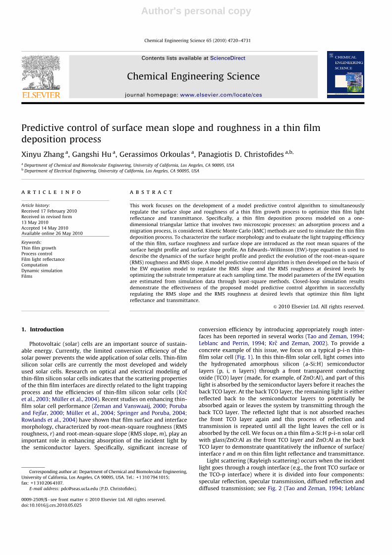
where N denotes the dimension of the approximation and thetilde symbols denote the association of these variables with afinite-dimensional system.

Fig. 10 shows the profiles of the reconstructed surfaceroughness square and mean slope square obtained from thefinite-dimensional approximations of Eq. (17) and compares themwith the values of the surface roughness square and of the meanslope square computed from the definitions of Eqs. (2) and (3). Itcan be seen from Fig. 10 that as the order of the approximationincreases, the reconstructed values are approaching the actualvalues computed from the definitions. Thus, the finite-dimensional approximation, that contains a finite number ofmodes, can be used for model prediction in the model predictivecontrol formulation. Note that, although a higher-order modelgenerally yields a more accurate approximation, the choice of thedimension of the reduced-order model is limited by the latticesize/discretization size. In the closed-loop simulations, the valuesof states are reconstructed from the discrete surface height profileby taking the inner product with the adjoint eigenfunctions. Dueto the finite number of discrete surface height points, there is alimited number (half of the discrete surface height points) ofstates (modes) that can be used to obtained correct estimates ofthe surface roughness square and of the mean slope square. Thislimited availability of the states is an additional reason for using areduced-order model in the MPC formulation. The MPC

0 20 40 60 80 1000.2

0.4

0.6

0.8

1

r2

Mode

0

20

40

60

80

m2

r2 (finite approximation)r2 (from surface profile)

m2 (finite approximation)m2 (from surface profile)

Fig. 10. Profiles of reconstructed surface roughness square and mean slope square

from the finite-dimensional approximation.



formulation based on the finite-dimensional approximation of theEW equation has the following form:

minT1 ,...,Ti ,...,Tp

J¼Xp

i ¼ 1

qm2 ,im2

set�/ ~m2ðtiÞS

m2set

" #2

þqr2 ,ir2

set�/~r2ðtiÞS

r2set

" #28<:

9=;

subject to /a2nðtiÞS¼�

s2

2lnþ a2

nðtÞþs2

2ln

� �e2lniD,

/~r2ðtiÞS¼

1

2L0

XN

n ¼ 1

/a2nðtiÞS,

/ ~m2ðtiÞS¼

XN

n ¼ 1

Kn/a2nðtiÞS,

TminoTioTmax, jðTiþ1�TiÞ=DjrLT ,

i¼ 1,2, . . . ,p: ð18Þ

5. Closed-loop simulations

In this section, we apply the proposed predictive controller of(18) to the kMC model of the thin film deposition process toregulate the surface slope and roughness at desired levels. Thesubstrate temperature is used as the manipulated variable, whichcan be implemented via a heating/cooling system. The adsorptionrate is kept constant during all deposition runs. The controlledvariables are the expected values of the mean slope square and ofthe surface roughness square at the end of the deposition process.

In the closed-loop simulations, the surface height profile isobtained from the surface morphology of the thin film from thekMC simulations and is transferred to the controller (statefeedback control) at each sampling time. A finite number of slowmodes are reconstructed from the surface height profile and areused to calculate the predictions of the mean slope square and ofthe surface roughness square along the prediction horizon. Theestimated parameters and the dependence of the parameters onsubstrate temperature is used when solving the optimizationproblem in the model predictive controller. The constrainedoptimization problem formulated in the MPC of (18) is solved andthe optimal input temperature profile is obtained and is applied tothe closed-loop system. The optimization problem is solved via alocal constrained minimization algorithm with a broad set ofinitial guesses. The measurement of thin film surface morphologyis a challenging issue, especially in real-time. Several techniqueshave been developed that enable surface height measurementsduring the operation of a deposition process like atomic forcemicroscopy. The surface information can be also obtained bycombining the on-line probing and off-line measurements.

After being computed from the solution of the optimizationproblem, the optimal manipulated input is applied to the thin filmgrowth process in a sample-and-hold fashion, i.e., the substratetemperature remains constant until the next sampling time. TheEW model constructed from the open-loop simulation data can beused in the MPC design since the manipulated input in the closed-loop system changes slowly with respect to the dynamics of theevolution of surface roughness and slope.

5.1. Separate regulation of surface slope and roughness

We first consider the control problems of separately regulatingsurface roughness and slope. Specifically, closed-loop simulationsof the slope-only control problem are carried out by assigning thefollowing values to the weighting factors in the MPC formulationof (18): qr2 ¼ 0:0 and qm2 ¼ 1:0. Two set-point values, m2

set¼0.5and 5, are considered. The order of finite-dimensional approx-imation used in the MPC formulation is N¼100. The depositionrate is fixed at W¼1 layer/s, which is appropriate from a practical

standpoint, and the initial substrate temperature is T¼500 K. Thevariation of temperature is from 400 to 700 K. The maximum rateof change of the temperature is LT¼1 K/s, which is also appro-priate from a practical standpoint. The number of prediction stepsis p¼5 and the prediction step size is D¼ 5 s. The sampling time isalso 5 s. Since the sampling time equals the prediction step size,only the first value of the manipulated input trajectory, T1, isapplied to the deposition process (i.e., kMC model) during thetime interval between two successive sampling times, ðt,tþDÞ. Atthe time tþD, the surface height profile is sampled and the MPCproblem of (16) is solved to obtain the next optimal manipulatedinput trajectory. The closed-loop simulation duration is 1000 s. Allexpected values are obtained from 200 independent simulationruns to evaluate the statistics of closed-loop performance.

Figs. 11 and 12 show, respectively, the profiles of the expectedmean slope square and of the expected substrate temperature inthe closed-loop simulation where the set-point of the mean slopesquare is 0.5. In Fig. 12, the substrate temperature increaseslinearly from the initial temperature of 500 K due to the constrainton the rate of change of the temperature. At large times

0 200 400 600 800 10000

1

2

3

4

5

6

Time (s)

<m2 >

Fig. 11. Profile of the expected mean slope square under closed-loop operation

(solid line); m2set¼0.5 (dashed line).

0 200 400 600 800 1000500

520

540

560

580

600

620

640

Time (s)

<T>

(K)

Fig. 12. Profile of the expected substrate temperature under closed-loop

operation; m2set¼0.5.



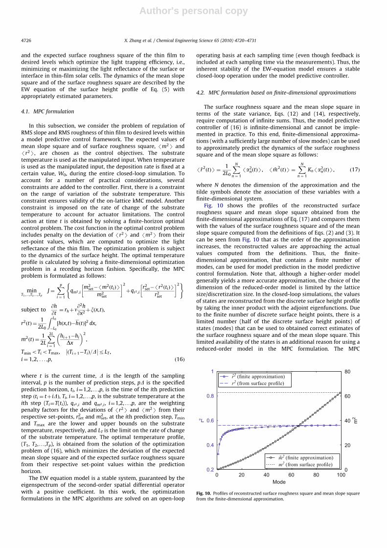
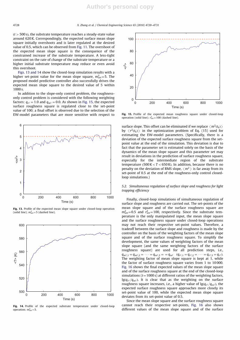
ðt4500 sÞ, the substrate temperature reaches a steady-state valuearound 620 K. Correspondingly, the expected surface mean slopesquare initially overshoots and is later regulated at the desiredvalue of 0.5, which can be observed from Fig. 11. The overshoot ofthe expected mean slope square is the consequence of theconstrained increase of the substrate temperature. A less-tightconstraint on the rate of change of the substrate temperature or ahigher initial substrate temperature may reduce or even avoidthis overshoot.

Figs. 13 and 14 show the closed-loop simulation results with ahigher set-point value for the mean slope square, m2

set¼5. Theproposed model predictive controller also successfully drives theexpected mean slope square to the desired value of 5 within1000 s.

In addition to the slope-only control problem, the roughness-only control problem is considered with the following weightingfactors: qr2 ¼ 1:0 and qm2 ¼ 0:0. As shown in Fig. 15, the expectedsurface roughness square is regulated close to the set-pointvalue of 100; a final offset is observed due to the selection of theEW-model parameters that are more sensitive with respect to

surface slope. This offset can be eliminated if we replace /m2ðtkÞSby /r2ðtkÞS in the optimization problem of Eq. (15) used forestimating the EW-model parameters. (Specifically, there is adeviation of the expected surface roughness square from the set-point value at the end of the simulation. This deviation is due tofact that the parameter set is estimated solely on the basis of thedynamics of the mean slope square and this parameter set mayresult in deviations in the prediction of surface roughness square,especially for the intermediate region of the substratetemperature ð500 KoTo650 KÞ. In addition, because there is nopenalty on the deviation of RMS slope, /m2S is far away from itsset-point of 0.5 at the end of the roughness-only control closed-loop simulations.)

5.2. Simultaneous regulation of surface slope and roughness for light

trapping efficiency

Finally, closed-loop simulations of simultaneous regulation ofsurface slope and roughness are carried out. The set-points of themean slope square and of the surface roughness square arem2

set¼0.5 and r2set¼100, respectively. Since the substrate tem-

perature is the only manipulated input, the mean slope squareand the surface roughness square under closed-loop operationsmay not reach their respective set-point values. Therefore, atradeoff between the surface slope and roughness is made by thecontroller on the basis of the weighting factors of the mean slopesquare and of the surface roughness square. To simplify thedevelopment, the same values of weighting factors of the meanslope square (and the same weighting factors of the surfaceroughness square) are used for all prediction steps, i.e.,qm2 ,1 ¼ qm2 ,2 ¼ � � � ¼ qm2 ,5 ¼ ¼ qm2 ðqr2 ,1 ¼ qr2 ,2 ¼ � � � ¼ qr2 ,5 ¼ qr2 Þ.The weighting factor of mean slope square is kept at 1, whilethe factor of surface roughness square varies from 1 to 10 000.Fig. 16 shows the final expected values of the mean slope squareand of the surface roughness square at the end of the closed-loopsimulations (t¼1000 s) at different ratios of the weighting factors,lgðqr2=qm2 Þ. It is clear that as the weighting on the surfaceroughness square increases, i.e., a higher value of lgðqr2=qm2 Þ, theexpected surface roughness square approaches more closely itsset-point value of 100, while the expected mean slope squaredeviates from its set-point value of 0.5.

Since the mean slope square and the surface roughness squarecannot reach their respective set-points, Fig. 16 also showsdifferent values of the mean slope square and of the surface

0 200 400 600 800 10000

1

2

3

4

5

6

Time (s)

<m2 >

Fig. 13. Profile of the expected mean slope square under closed-loop operation

(solid line); m2set¼5 (dashed line).

0 200 400 600 800 1000500

520

540

560

580

600

Time (s)

<T>

(K)

Fig. 14. Profile of the expected substrate temperature under closed-loop

operation; m2set¼5.

0 200 400 600 800 10000

20

40

60

80

100

Time (s)

<r2 >

Fig. 15. Profile of the expected mean roughness square under closed-loop

operation (solid line); r2set¼100 (dashed line).



roughness square which are obtained at the end of the closed-loop simulations with different weighting factors of the meanslope square and of the surface roughness square. The lightreflectance of these thin films obtained from the closed-loopsimulations of simultaneous regulation can be computed from theresulting RMS surface slope and RMS roughness using Eq. (1), asshown in Fig. 17. In Fig. 17, the RMS slope, m, and the RMSroughness, r, are computed as the square roots of /m2S and /r2S,respectively. The RMS roughness is also scaled with (bymultiplying) a physical factor, 6.5 nm, so that the set-pointvalue, r2

set, together with m2set, corresponds to an optimal value

(maximum) of the light reflectance in Eq. (1).It can be seen from Fig. 17 that different values of light

reflectance of thin film are obtained at different ratios of theweighting factors, lgðqr2=qm2 Þ. A plot with contours of the lightreflectance is given in Fig. 18, which shows the dependence of theRMS slope, the RMS roughness, and the corresponding lightreflectance of the thin film on the weighting factors. We note thatthe values of the RMS roughness in Figs. 17 and 18 are also scaled

with the same factor as the one for r2set. An optimal weighting

scheme can be determined based on Figs. 17 and 18. For example,in the case where a high light reflectance is desired to improve thelight trapping efficiency (e.g., for the back TCO layer that reflectsthe transmitted light back to the p-i-n layers of the thin film), acombination of the weighting factors, qr2 ¼ 1 and qm2 ¼ 1, can beused in the closed-loop operation.

For a perspective of the surface morphology of the thin films,representative snapshots of the film surface microstructure at theend of single open-loop and closed-loop simulations (t¼1000 s)are shown in Fig. 19. Three closed-loop cases are compared: (1)slope-only control, (2) roughness-only control, and (3) andsimultaneous control of slope and roughness. It can bee seen inFig. 19 that different values of the mean slope square and of thesurface roughness square are achieved at the end of simulations. Inthe open-loop simulation, the substrate temperature and theadsorption rate are fixed and the surface slope and roughnessevolve following the open-loop dynamics. In the slope-only androughness-only control, the mean slope square and the surfaceroughness square are regulated around their respective set-pointvalues, m2

set¼0.5 and r2set¼100, at the end of the simulation. In the

case of simultaneous control of slope and roughness, a trade-off ismade between the mean slope square and the surface roughnesssquare. Specifically, different surface height profiles can beobserved in Fig. 19 under open-loop operation and underdifferent closed-loop operations. A nearly smooth surface heightprofile is obtained under slope-only control with a low RMS slope(since the RMS slope set-point, 0.5, is quite low) and a certain levelof RMS roughness; these values of RMS slope and roughness resultin a reflectance value of R/R0¼0.69 which could be appropriate fora back TCO layer. On the other hand, roughness-only controlresults in a rough surface height profile with both large slopefluctuation (high RMS slope) and large height fluctuation (highRMS roughness); these values of RMS slope and roughness resultin a reflectance value of R/R0¼0.18 which could be appropriate fora front TCO layer. The surface height profile under simultaneouscontrol of slope and roughness with weighting factor ratiolgðqr2=qm2 Þ ¼ 3 results in an ‘‘intermediate’’ surface height profile,as can be seen in Fig. 19, between slope-only control androughness-only control, and a reflectance value of R/R0¼0.46which could be appropriate for an intermediate solar cell layer.Therefore, by appropriately choosing the set-points for RMS

0 1 2 3 40

20

40

60

80

100

<r2 >

lg(qr2/qm

2)

0

0.5

1

1.5

2

2.5

<m2 >

<r2>

<m2>

Fig. 16. Profiles of /r2S (solid line) and /m2S (dashed line) at the end of closed-

loop simulations (t¼1000 s) for different penalty weighting factors: qm2 ¼ 1 and

1rqr2 r10 000.

0 1 2 3 4

0.4

0.5

0.6

0.7

0.8

lg(qr2/qm2)

R/R

0

Fig. 17. Dependence of light reflectance of thin film on the ratio of the weighting

factors, lgðqr2 =qm2 Þ; r2set¼100 and m2

set¼0.5.

m

r (m

)

0.5 1 1.5 2 2.5 3

1

2

3

4

5

6

7

8

9

x 10−8

0.1

0.2

0.3

0.4

0.5

0.6

0.7

0.8

0.9

Fig. 18. Light reflectance of thin films deposited under closed-loop operations

with different weighting schemes.



roughness and RMS slope as well as the weighting factors, we canproduce layers that have a broad range of reflectance values.

Remark 3. In this work, the expected values of roughness andslope are compared to their respective set-points at the end of thedeposition (t¼1000 s). The film thickness is not considered as acontrol objective. In some applications, there are stringentrequirements for specific film thickness. If this is the case, modelpredictive controllers can be developed for simultaneous regula-tion of surface roughness, film porosity, and film thickness byincluding cost penalty on the deviation of film thickness from adesired minimum value or by implementing the thicknessrequirement as a constraint (Hu et al., 2009c; Zhang et al., inpress).

6. Conclusions

A model predictive control algorithm was developed toregulate the surface slope and roughness of a thin film growthprocess. The thin film deposition process was modeled on a one-dimensional triangular lattice that involves two microscopicprocesses: an adsorption process and a migration process. Kinetic

Monte Carlo methods were used to simulate the thin filmdeposition process. To characterize the surface morphology andto evaluate the light trapping efficiency of the thin film, surfaceroughness and surface slope were introduced as the root meansquares of the surface height profile and surface slope profile. AnEW-type equation was used to describe the dynamics of thesurface height profile and predict the evolution of the RMSroughness and RMS slope. A model predictive control algorithmwas then developed on the basis of the EW equation model tosimultaneously regulate the RMS slope and the RMS roughness atdesired levels by optimizing the substrate temperature at eachsampling time. The model parameters of the EW equation wereestimated from simulation data through least-square methods.Closed-loop simulation results were presented to demonstrate theeffectiveness of the proposed model predictive control algorithmin successfully regulating the RMS slope and the RMS roughnessat desired levels that optimize thin film light reflectance andtransmittance.

Acknowledgment

Financial support from NSF, CBET-0652131, is gratefullyacknowledged.

References

Bennett, H.E., Porteus, J.O., 1961. Relation between surface roughness and specularreflectance at normal incidence. Journal of the Optical Society of America 51,123–129.

Christofides, P.D., Armaou, A., Lou, Y., Varshney, A., 2008. Control and Optimizationof Multiscale Process Systems. Birkhauser, Boston.

Davies, H., 1954. The reflection of electromagnetic waves from a rough surface.Proceedings of the Institution of Electrical Engineers 101, 209.

Edwards, S.F., Wilkinson, D.R., 1982. The surface statistics of a granular aggregate.Proceedings of the Royal Society of London Series A—Mathematical Physicaland Engineering Sciences 381, 17–31.

Family, F., 1986. Scaling of rough surfaces: effects of surface diffusion. Journal ofPhysics A: Mathematical and General 19, L441–L446.

Hu, G., Huang, J., Orkoulas, G., Christofides, P.D., 2009a. Investigation of filmsurface roughness and porosity dependence on lattice size in a porous thinfilm deposition process. Physical Review E 80, 041122.

Hu, G., Orkoulas, G., Christofides, P.D., 2009b. Modeling and control of film porosityin thin film deposition. Chemical Engineering Science 64, 3668–3682.

Hu, G., Orkoulas, G., Christofides, P.D., 2009c. Regulation of film thickness, surfaceroughness and porosity in thin film growth using deposition rate. ChemicalEngineering Science 64, 3903–3913.

Hu, G., Orkoulas, G., Christofides, P.D., 2009d. Stochastic modeling and simulta-neous regulation of surface roughness and porosity in thin film deposition.Industrial & Engineering Chemistry Research 48, 6690–6700.

Huang, J., Hu, G., Orkoulas, G., Christofides, P.D., Dynamics and lattice-sizedependence of surface mean slope in thin film deposition. Industrial &Engineering Chemistry Research, in press, doi:10.1021/ie10012w.

Krc, J., Smole, F., Topic, M., 2003. Analysis of light scattering in amorphous Si:Hsolar cells by a one-dimensional semi-coherent optical model. Progress inPhotovoltaics: Research and Applications 11, 15–26.

Krc, J., Zeman, M., 2002. Experimental investigation and modelling of lightscattering in a-Si:H solar cells deposited on glass/ZnO:Al substrates. MaterialResearch Society 715, A13.3.1–A13.3.6.

Krc, J., Zeman, M., 2004. Optical modeling of thin-film silicon solar cells depositedon textured substrates. Thin Solid Films 451, 298–302.

Leblanc, F., Perrin, J., 1994. Numerical modeling of the optical properties ofhydrogenated amorphous-silicon-based p-i-n solar cells deposited onrough transparent conducting oxide substrates. Journal of Applied Physics75, 1074.

Levine, S.W., Clancy, P., 2000. A simple model for the growth of polycrystalline Siusing the kinetic Monte Carlo simulation. Modelling and Simulation inMaterials Science and Engineering 8, 751–762.

Levine, S.W., Engstrom, J.R., Clancy, P., 1998. A kinetic Monte Carlo study of thegrowth of Si on Si(1 0 0) at varying angles of incident deposition. SurfaceScience 401, 112–123.

Muller, J., Rech, B., Springer, J., Vanecek, M., 2004. TCO and light trapping in siliconthin film solar cells. Solar Energy 77, 917–930.

Ni, D., Christofides, P.D., 2005. Multivariable predictive control of thin filmdeposition using a stochastic PDE model. Industrial & Engineering ChemistryResearch 44, 2416–2427.

0 20 40 60 80 100

1260

1280

1300Open−loop: r2 = 131.1, m2 = 19.62, R/R0=0.10

Hei

ght (

laye

rs)

0 20 40 60 80 100

960

980

1000

Slope−only control: r2 = 19.0, m2 = 0.57, R/R0=0.69

Hei

ght (

laye

rs)

0 20 40 60 80 100

1340

1360

1380

Roughness−only control: r2 = 83.0, m2 = 20.79, R/R0=0.18

Hei

ght (

laye

rs)

Hei

ght (

laye

rs)

Width (sites)0 20 40 60 80 100

960

980

1000

Slope and roughness control: r2=59.3, m2=0.78, R/R0=0.46

Fig. 19. Snapshots of the film microstructure at the end of simulations (t¼1000 s)

under open-loop and closed-loop operations. The open-loop operating conditions:

T ¼ 500 K and W¼1.0 layer/s; the set-points in closed-loop simulation: r2set¼100

and m2set¼0.5; the weighting factor ratio in the simultaneous regulation:

lgðqr2=qm2 Þ ¼ 3.



Poruba, A., Fejfar, A., 2000. Optical absorption and light scattering in microcrystal-line silicon thin films and solar cells. Journal of Applied Physics 88,148–160.

Rowlands, S.F., Livingstone, J., Lund, C.P., 2004. Optical modelling of thin film solarcells with textured interfaces using the effective medium approximation. SolarEnergy 76, 301–307.

Springer, J., Poruba, A., 2004. Improved three-dimensional optical model for thin-film silicon solar cells. Journal of Applied Physics 96, 5329–5337.

Tao, G., Zeman, M., 1994. Optical modeling of a-Si:H based solar cells on texturedsubstrates. In: 1994 IEEE First World Conference on Photovoltaic EnergyConversion. Conference Record of the 24th IEEE Photovoltaic SpecialistsConference-1994 (Cat. no. 94CH3365-4), vol. 1, p. 666.

Varshney, A., Armaou, A., 2005. Multiscale optimization using hybrid PDE/kMCprocess systems with application to thin film growth. Chemical EngineeringScience 60, 6780–6794.

Varshney, A., Armaou, A., 2006. Identification of macroscopic variables for low-order modeling of thin-film growth. Industrial & Engineering ChemistryResearch 45, 8290–8298.

Varshney, A., Armaou, A., 2008. Reduced order modeling and dynamic optimiza-tion of multiscale pde/kmc process systems. Computers & Chemical Engineer-ing 32, 2136–2143.

Vlachos, D.G., Schmidt, L.D., Aris, R., 1993. Kinetics of faceting of crystals in growth,etching, and equilibrium. Physical Review B 47, 4896–4909.

Wang, L., Clancy, P., 2001. Kinetic Monte Carlo simulation of the growth ofpolycrystalline Cu films. Surface Science 473, 25–38.

Yang, Y.G., Johnson, R.A., Wadley, H.N.G., 1997. A Monte Carlo simulation of thephysical vapor deposition of nickel. Acta Materialia 45, 1455–1468.

Zeman, M., Vanswaaij, R., 2000. Optical modeling of a-Si:H solar cells with roughinterfaces: effect of back contact and interface roughness. Journal of AppliedPhysics 88, 6436–6443.

Zhang, P., Zheng, X., Wu, S., Liu, J., He, D., 2004. Kinetic Monte Carlo simulation ofCu thin film growth. Vacuum 72, 405–410.

Zhang, X., Hu, G., Orkoulas, G., Christofides, P.D., Controller and estimator designfor regulation of film thickness, surface roughness and porosity in a multiscalethin film growth process. Industrial & Engineering Chemistry Research, inpress, doi:10.1021/ic901396g.


Documents

Author's personal copy - University of California, Los …pdclab.seas.ucla.edu/Publications/XZhang/XZhang_GHu_GOrkoulas_PD...Author's personal copy Predictive control of surface mean