Author's personal copy - CHRSs personal copy Watershed rainfall forecasting using neuro-fuzzy ... Rainfall forecasting Arti cial Neural Network ... commonly coupled with heavy rainfall

Author's personal copy

Watershed rainfall forecasting using neuro-fuzzy networkswith the assimilation of multi-sensor information

Fi-John Chang a,⇑, Yen-Ming Chiang b, Meng-Jung Tsai a, Ming-Chang Shieh c, Kuo-Lin Hsu d,Soroosh Sorooshian d

a Department of Bioenvironmental Systems Engineering, National Taiwan University, Taipei, Taiwanb Department of Hydraulic Engineering, Zhejiang University, Hangzhou, Chinac Water Resources Agency, Ministry of Economic Affairs, Taipei, Taiwand Center for Hydrometeorology and Remote Sensing, Department of Civil and Environmental Engineering, University of California, Irvine, CA, USA

a r t i c l e i n f o

Article history:Received 25 June 2013Received in revised form 9 October 2013Accepted 9 November 2013Available online 19 November 2013This manuscript was handled byKonstantine P. Georgakakos, Editor-in-Chief,with the assistance of Hervé AndrieuAssociate Editor

Keywords:Data mergingData assimilationRadarSatelliteRainfall forecastingArtificial Neural Network

s u m m a r y

The complex temporal heterogeneity of rainfall coupled with mountainous physiographic context makesa great challenge in the development of accurate short-term rainfall forecasts. This study aims to explorethe effectiveness of multiple rainfall sources (gauge measurement, and radar and satellite products) forassimilation-based multi-sensor precipitation estimates and make multi-step-ahead rainfall forecastsbased on the assimilated precipitation. Bias correction procedures for both radar and satellite precipita-tion products were first built, and the radar and satellite precipitation products were generated throughthe Quantitative Precipitation Estimation and Segregation Using Multiple Sensors (QPESUMS) and thePrecipitation Estimation from Remotely Sensed Information using Artificial Neural Networks-Cloud Clas-sification System (PERSIANN-CCS), respectively. Next, the synthesized assimilated precipitation wasobtained by merging three precipitation sources (gauges, radars and satellites) according to their individ-ual weighting factors optimized by nonlinear search methods. Finally, the multi-step-ahead rainfall fore-casting was carried out by using the adaptive network-based fuzzy inference system (ANFIS). TheShihmen Reservoir watershed in northern Taiwan was the study area, where 641 hourly data sets of thir-teen historical typhoon events were collected. Results revealed that the bias adjustments in QPESUMSand PERSIANN-CCS products did improve the accuracy of these precipitation products (in particular,30–60% improvement rates for the QPESUMS, in terms of RMSE), and the adjusted PERSIANN-CCS andQPESUMS individually provided about 10% and 24% contribution accordingly to the assimilated precipi-tation. As far as rainfall forecasting is concerned, the results demonstrated that the ANFIS fed with theassimilated precipitation provided reliable and stable forecasts with the correlation coefficients higherthan 0.85 and 0.72 for one- and two-hour-ahead rainfall forecasting, respectively. The obtained forecast-ing results are very valuable information for the flood warning in the study watershed during typhoonperiods.

� 2013 Elsevier B.V. All rights reserved.

1. Introduction

Rainfall is a key hydrological variable that links the atmosphereand land surface processes. The complex temporal heterogeneity oftyphoon rainfall coupled with mountainous physiographic contextmakes the development of accurate forecasting reservoir inflowseveral hours ahead of time a great challenge. Typhoons arecommonly coupled with heavy rainfall. For instance, the highestrainfall record of Typhoon Morakot was over 1000 mm/day insouthern Taiwan in 2009. Due to abundant rainwater, the inunda-tion disaster occurred in most of this area and caused more than

USD 0.5 billion losses. The fatally rainfall-induced landslide buriedthe entire Shaoling village, which killed about 500 people in thevillage alone. Consequently short-term typhoon rainfall forecastingis recognized as the most important study for reservoir watershedmanagement and flood mitigation in Taiwan. As far as rainfall fore-casting is concerned, the accuracy of precipitation products andtheir nowcasting is continuously improved and becomes more reli-able for practical applications in recent years. For example, Koberet al. (2012) blended a probabilistic nowcasting method with ahigh-resolution numerical weather prediction assimilated for con-vective precipitation forecasts. Haiden et al. (2011) presented theintegrated nowcasting through a comprehensive analysis systemand provided the products of precipitation amount and types.Sokol (2006) applied a multiple linear regression model

0022-1694/$ - see front matter � 2013 Elsevier B.V. All rights reserved.http://dx.doi.org/10.1016/j.jhydrol.2013.11.011

⇑ Corresponding author. Tel.: +886 2 23639461; fax: +886 2 23635854.E-mail address: [email protected] (F.-J. Chang).

Journal of Hydrology 508 (2014) 374–384

Contents lists available at ScienceDirect

Journal of Hydrology

journal homepage: www.elsevier .com/locate / jhydrol


complemented by a correction procedure for nowcasting of 1-hprecipitation using radar and numerical weather prediction data.Sokol and Pesice (2012) proposed a model SAM for nowcasting 1to 3-h precipitation totals and improved forecasts accuracy. Zah-raei et al. (2012) introduced a pixel-based algorithm for short-termquantitative precipitation forecasting using radar-based rainfalldata and shown promising performance in severe stormsforecasting.

Precipitation observations, in general, are available from severalsources, such as ground rain gauges, radars and satellites. Thesesources not only have significant differences in both spatial andtemporal resolutions but also have different limitations subjectto hardware mechanisms. Ground gauges observe surface precipi-tation continuously and directly, however, gauges are sparsely lo-cated and only provide point-scale measurements, which implythe spatial representation of gauges is weak. Radars use reflectedmicrowave energy to derive precipitation at a height betweenabout 500 m and 5000 m above sea level, however, radar coverageis many times limited by orography. Satellites, whose coverage isnot limited by orography, provide rapid precipitation informationover large areas. However, satellite measurements not only areindirectly related to surface precipitation but also have lower spa-tial and temporal resolutions, as compared to those of radar prod-ucts. On account of the different strengths and weaknesses of eachmeasurement technology, a potential advantage is thereby to inte-grate precipitation measurements from different measurementapparatuses such as gauges, radars and satellites for improvingthe accuracy of rainfall forecast (Grecu and Krajewski, 2000; Kiddet al., 2003; Chiang et al., 2007a; Mittermaier, 2008).

The Artificial Neural Network (ANN) was inspired by neurobiol-ogy to perform brain-like computations and has been recognizedas an effective tool for modeling complex nonlinear systems inthe last two decades. The applications of ANNs to various aspectsof hydrological modeling have provided many promising results,such as rainfall estimation/prediction (Hong et al., 2005, 2006;Chiang et al., 2007a; Chen et al., 2011), flood forecasting (Chiangand Chang, 2009; Siou et al., 2011; Yilmaz et al., 2011), and waterlevel prediction (Chiang et al., 2010; Adamowski and Chan, 2011).Neuro-fuzzy systems that combine ANNs and fuzzy theories haveproven to be another powerful intelligent system and havereceived much attention in recent years (Chang et al., 2005;Coulibaly and Evora, 2007; Firat, 2008; Lohani et al., 2011). BothANNs and fuzzy theories have been developed to simulate thethinking process of human brain for learning similar strategies orexperiences to make optimal decisions. Nevertheless, the funda-mental mechanisms of these two theories are different, in whichANNs offer a superior capability to extract significant features fromcomplex databases and are capable of learning the relationshipbetween any data pairs, whereas the fuzzy logic is based on theway how brains deal with inexact information. Due to the lack oflearning capability for fuzzy theories, it is difficult to tune the fuzzyrules and membership functions based on training data. Therefore,the neuro-fuzzy system was developed for capturing the advanta-ges and strengths of both ANNs and fuzzy logic in a single frame-work. The adaptive network-based fuzzy inference system(ANFIS), proposed by Jang (1993), is one of the famous neuro-fuzzysystems and has been applied to modeling daily discharge re-sponses (Kurtulus and Razack, 2010), water level prediction(Chiang et al., 2011), and rainfall-runoff simulations (Shu andOuarda, 2008).

This study aims at providing reliable and accurate short-termtyphoon rainfall forecasts using artificial intelligent (AI) techniquesbased on the assimilation of satellite- and radar-derived rainfallestimations and ground gauge measurements. The organizationof this paper is addressed as follows. The description of the studyarea, ground measurements, radar-derived and satellite-derived

precipitation estimation as well as the model construction is pro-vided in Section 2. Section 3 presents the methodologies, includingthe back-propagation neural network (BPNN) for bias adjustment,the genetic algorithm (GA) for data merge, and the ANFIS for rain-fall forecasting. Section 4 shows the results and comparison of twobias correction strategies, the effectiveness of merging precipita-tion products, and the performance of rainfall forecasting. Finally,the conclusions are given in Section 5.

2. Materials

2.1. Study area and gauging station datasets

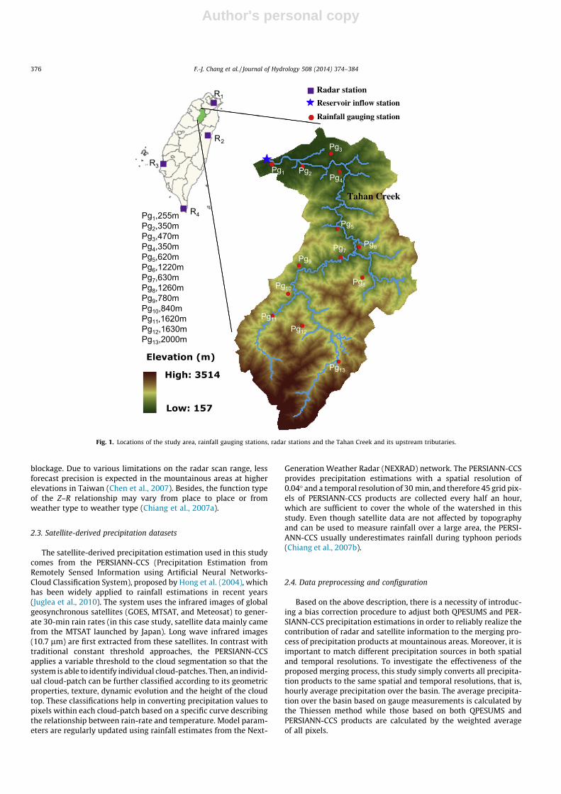
The study area of this study belongs to the Shihmen Reservoirwatershed and is located on the upstream of the Tahan River innorthern Taiwan. Fig. 1 shows the locations of the Shihmen Reser-voir watershed where the reservoir inflow gauging station isdenoted with a blue1 star, each radar station is denoted with a purplesquare, and each of thirteen rain gauging stations is denoted with a reddot. All the thirteen rain gauging stations are spatially well distributedbelow 2000 m in elevation. Under this condition, no rain gauge is setup above 2000 m. Alternatively, remote sensing, such as radar and sa-tellite, is considered to provide rainfall information for areas above2000 m. This watershed receives an annual rainfall of about2500 mm, which mainly comes from typhoons. Because rainwaterusually occurs in a short duration with great intensity, heavy rainfallcoupled with huge runoff would flows into the Reservoir in just a cou-ple of hours. Consequently, reliable typhoon rainfall forecasting playsan important role in reservoir operation and management because ty-phoons usually affect Taiwan for about 3–5 days. Four types of data,including reservoir inflow (m3/s), rain gauge measurements (mm),and radar- and satellite-derived precipitation estimations (mm) werecollected from 2006 to 2009 in this study. A total of 641 hourly dataassociated with thirteen historical typhoon events were obtained.

2.2. Radar-derived precipitation datasets

The radar-derived precipitation estimation applied in this studycan be referred to the QPESUMS (Quantitative Precipitation Esti-mation and Segregation Using Multiple Sensors) system (http://qpesums.cwb.gov.tw/taiwan-html2/), which was developed bythe Central Weather Bureau (CWB) of Taiwan and the NationalSevere Storms Laboratory (NSSL) of National Oceanic and Atmo-spheric Agency (NOAA) of the USA. The QPESUMS system mainlycomposes of four weather Doppler radars that cover the whole ofTaiwan and the adjacent ocean, and it records base reflectivity witha spatial resolution of 0.0125� in both longitude and latitude and atemporal resolution of 10 min. The R1 radar station has the shortestdistance to the study area (less than 80 km) and is located at lon-gitude 121.46�E and latitude 25.04�N with an elevation of 760 m.This radar belongs to the Weather Surveillance Radar 1988 Doppler(WSR-88D) with a wavelength of 10 cm (S-band) and performsapproximately 10 different elevation scans (between 0.5� and 15�above the horizon) that consist of a complete volume scan. Thebeam width is 0.857�. The system generates the constant altitudeplan position indicators (CAPPI) at the elevation of 1000 m andestimates rainfall using the Z–R relation with the function typeZ = 32.5R1.65. Therefore, the records of 434 grid pixels are collectedto cover the whole of the watershed for every 10 min. Even thoughthe QPESUMS system is used to monitor rainfall in Taiwan, the Z–Rrelationship for converting radar reflectivity to rainfall rates can beaffected by various problems, such as ground clutter and beam

1 For interpretation of color in Figs. 1 and 5, the reader is referred to the webversion of this article.

F.-J. Chang et al. / Journal of Hydrology 508 (2014) 374–384 375


blockage. Due to various limitations on the radar scan range, lessforecast precision is expected in the mountainous areas at higherelevations in Taiwan (Chen et al., 2007). Besides, the function typeof the Z–R relationship may vary from place to place or fromweather type to weather type (Chiang et al., 2007a).

2.3. Satellite-derived precipitation datasets

The satellite-derived precipitation estimation used in this studycomes from the PERSIANN-CCS (Precipitation Estimation fromRemotely Sensed Information using Artificial Neural Networks-Cloud Classification System), proposed by Hong et al. (2004), whichhas been widely applied to rainfall estimations in recent years(Juglea et al., 2010). The system uses the infrared images of globalgeosynchronous satellites (GOES, MTSAT, and Meteosat) to gener-ate 30-min rain rates (in this case study, satellite data mainly camefrom the MTSAT launched by Japan). Long wave infrared images(10.7 lm) are first extracted from these satellites. In contrast withtraditional constant threshold approaches, the PERSIANN-CCSapplies a variable threshold to the cloud segmentation so that thesystem is able to identify individual cloud-patches. Then, an individ-ual cloud-patch can be further classified according to its geometricproperties, texture, dynamic evolution and the height of the cloudtop. These classifications help in converting precipitation values topixels within each cloud-patch based on a specific curve describingthe relationship between rain-rate and temperature. Model param-eters are regularly updated using rainfall estimates from the Next-

Generation Weather Radar (NEXRAD) network. The PERSIANN-CCSprovides precipitation estimations with a spatial resolution of0.04� and a temporal resolution of 30 min, and therefore 45 grid pix-els of PERSIANN-CCS products are collected every half an hour,which are sufficient to cover the whole of the watershed in thisstudy. Even though satellite data are not affected by topographyand can be used to measure rainfall over a large area, the PERSI-ANN-CCS usually underestimates rainfall during typhoon periods(Chiang et al., 2007b).

2.4. Data preprocessing and configuration

Based on the above description, there is a necessity of introduc-ing a bias correction procedure to adjust both QPESUMS and PER-SIANN-CCS precipitation estimations in order to reliably realize thecontribution of radar and satellite information to the merging pro-cess of precipitation products at mountainous areas. Moreover, it isimportant to match different precipitation sources in both spatialand temporal resolutions. To investigate the effectiveness of theproposed merging process, this study simply converts all precipita-tion products to the same spatial and temporal resolutions, that is,hourly average precipitation over the basin. The average precipita-tion over the basin based on gauge measurements is calculated bythe Thiessen method while those based on both QPESUMS andPERSIANN-CCS products are calculated by the weighted averageof all pixels.

Reservoir inflow station

Rainfall gauging station

Pg1 Pg2 Pg4

Pg12

Pg11

Pg13

Pg9

Pg7

Pg10Pg8

Pg6

Pg5

Pg3

Pg1,255mPg2,350mPg3,470mPg4,350mPg5,620mPg6,1220mPg7,630mPg8,1260mPg9,780mPg10,840mPg11,1620mPg12,1630mPg13,2000m

Radar stationR1

R2

R3

R4

Tahan Creek

Fig. 1. Locations of the study area, rainfall gauging stations, radar stations and the Tahan Creek and its upstream tributaries.

376 F.-J. Chang et al. / Journal of Hydrology 508 (2014) 374–384


As for the configuration of thirteen typhoon events, 7 eventswith 350 hourly data were arranged in the training phase for cali-brating the model structure and parameters, 3 events with 153hourly data were arranged in the validation phase for determiningthe training epochs in order to avoid over-fitting problems, and theremaining 3 events with 138 hourly data were arranged in the test-ing phase for evaluating the performance and generalization capa-bility of the determined network. Table 1 shows the statistics ofthese three independent datasets.

3. Methodology

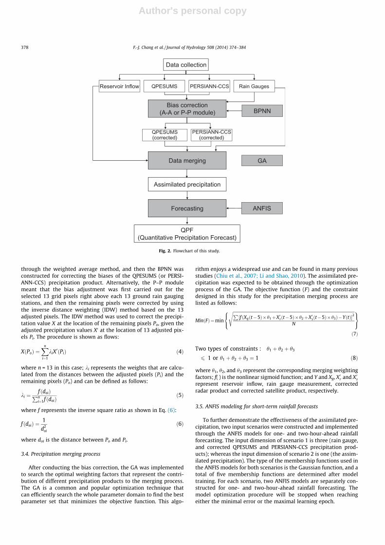
A novel approach that comprises two main parts is proposed:(1) the bias correction and the assimilation of multi-sensor rainfallinformation using the BPNN and the GA, respectively; and (2) theconstruction of multi-step-ahead rainfall forecasting through theANFIS. The first part is mainly to explore the effectiveness of assim-ilating multiple rainfall sources (satellite precipitation product,radar precipitation product and ground gauge measurements),and the second part intends to provide reliable and accurate1–2 h-ahead rainfall forecasts based on the assimilated precipita-tion. Fig. 2 illustrates the schematic flowchart of this study. Thedetailed procedures and a brief introduction of the implementationmethods, i.e., BPNN and ANFIS, are given as follows:

3.1. Back-propagation neural network (BPNN)

The BPNN is widely used for hydrological modeling and hasreceived numerous successes in simulations and predictions. TheBPNN has unique advantages such as the excellent convergencecapability. The steepest descent method is one of the algorithmsthat are frequently adopted for training the BPNN, but, however,it often suffers from local optimizations. To overcome this problem,the conjugate gradient algorithm has now become much popularbecause it represents a compromise between the simplicity ofthe steepest descent method and the fast quadratic convergenceof the Newton’s method. In general, the conjugate gradient algo-rithm makes a good uniform progress toward the solution at eachstep and has been found to be effective in searching a better solu-tion than the steepest descent method (Haykin, 1999; Chiang et al.,2004). Therefore, the conjugate gradient algorithm was applied inthis study for model calibration.

3.2. Adaptive network-based fuzzy inference system (ANFIS)

The ANFIS has received much attention because of its outstand-ing capability of learning any real continuous function. The ANFISnot only maintains the learning ability of ANNs for mapping aninput space onto an output space but also possesses the advanta-ges of fuzzy if-then rules for describing the local behavior of suchmapping. The system results can then be obtained through the rea-soning capability of fuzzy logics. The architecture of the ANFIS con-sists of five layers, and the training of the ANFIS can be referred to ahybrid learning algorithm, that is, an incorporation of the gradient

descent method and the least-squares method. Furthermore, thedetermination of the number of fuzzy rules is an important stepwhen applying the ANFIS. When the number of rules increases,the number of parameters determined will become enormous,which will consume considerable computational time and, evenworse, result in decreasing the capability of generalization. Tosolve this problem, the fuzzy subtractive clustering algorithm isadopted for establishing the relationship between input and out-put variables. The fuzzy subtractive clustering algorithm can effec-tively distinguish the fuzzy qualities associated with each of theclusters through the minimum number of rules. Details of the AN-FIS modeling with the fuzzy subtractive clustering can be found inChang and Chang (2001).

3.3. BPNN modeling for bias corrections

According to the correlation analysis between reservoir inflowand all rain gauges at different lag times, it suggested that the timeof concentration in the study area was about 5–7 h. Nevertheless,the inflow prediction could merely be performed at a lead timeof 5 h only if observations were available. In other words, rainfallforecasting at lead times of 1 and 2 h should be provided if theinflow prediction is required for a lead time of 7 h. Eq. (1) showsthe relationship between rainfall and inflow when constructingthe rainfall–runoff model.

Yðt þ nÞ ¼ f ðXgðt þ n� 5Þ; Xgðt þ n� 6Þ; Xgðt þ n� 7ÞÞ ð1Þ

where Y and Xg denote reservoir inflow and rain gauge measure-ments, respectively. The f( ) is a nonlinear transfer function, i.e., asigmoid function, and t and n are current time and forecast leadtime, respectively.

To correct the bias of each precipitation product, the BPNN wasused to find the nonlinear function. Two independent BPNNs wereseparately fed with uncorrected QPESUMS and PERSIANN-CCS pre-cipitation data for fitting the ground gauge values of training data-sets. As far as the model setting was concerned, the BPNNconsisted of three layers: an input layer with a single input (QPE-SUMS or PERSIANN-CCS precipitation data); a hidden layer withhidden nodes determined by trial-and-error (usually less than 5nodes); and an output layer with a single output (corrected rainfall(X0)). The optimization/stop criteria included the minimal error(0.0001 mm/h) and the number of learning iterations (1000). Themodel optimization procedure would stop when reaching eitherof the two criteria. Because the direct outputs of the model mightnot provide a meaningful representation as compared with thoseof the original QPESUMS and PERSIANN-CCS precipitation prod-ucts, it was necessary to specifically present the biases and randomerrors of the original QPESUMS and PERSIANN-CCS precipitationproducts. Therefore, coefficients a and b were assumed for the pur-pose of transforming the BPNN outputs into the following formats:

X0rðtÞ ¼ a1XrðtÞ þ b1 ð2Þ

X0sðtÞ ¼ a2XsðtÞ þ b2 ð3Þ

where X 0r and X0s represent the corrected radar and satellite products(BPNN outputs), respectively. a and b represent the random andbias errors of uncorrected (original) radar and satellite precipitationproducts (Xr and Xs, respectively).

The bias correction procedure consisted of two modules (area toarea (A–A) and point to point (P–P) modules), which investigatedthe influence of spatial resolution of rainfall on the bias correction.The A–A module meant that the bias correction was performedwith a basin-scale average precipitation product. In other words,the A–A module simply calculated the average precipitation overthe basin based on the QPESUMS (or PERSIANN-CCS) products

Table 1Statistics of ground precipitation measurements in different datasets.

Event (a) Max. Min. Meanb SDc

Training 7 (350) 44.4 0 6.5 8.2Validation 3 (153) 33.2 0 4.3 6.2Testing 3 (138) 26.9 0 5.1 6.2

a Number of data.b Unit (mm/h).c Standard deviation.



through the weighted average method, and then the BPNN wasconstructed for correcting the biases of the QPESUMS (or PERSI-ANN-CCS) precipitation product. Alternatively, the P–P modulemeant that the bias adjustment was first carried out for theselected 13 grid pixels right above each 13 ground rain gaugingstations, and then the remaining pixels were corrected by usingthe inverse distance weighting (IDW) method based on the 13adjusted pixels. The IDW method was used to correct the precipi-tation value X at the location of the remaining pixels Po, given theadjusted precipitation values X0 at the location of 13 adjusted pix-els Pi. The procedure is shown as flows:

XðPoÞ ¼Xn

i¼1

kiX0ðPiÞ ð4Þ

where n = 13 in this case; ki represents the weights that are calcu-lated from the distances between the adjusted pixels (Pi) and theremaining pixels (Po) and can be defined as follows:

ki ¼f ðdoiÞPni¼1f ðdoiÞ

ð5Þ

where f represents the inverse square ratio as shown in Eq. (6):

f ðdoiÞ ¼1

d2oi

ð6Þ

where doi is the distance between Po and Pi.

3.4. Precipitation merging process

After conducting the bias correction, the GA was implementedto search the optimal weighting factors that represent the contri-bution of different precipitation products to the merging process.The GA is a common and popular optimization technique thatcan efficiently search the whole parameter domain to find the bestparameter set that minimizes the objective function. This algo-

rithm enjoys a widespread use and can be found in many previousstudies (Chiu et al., 2007; Li and Shao, 2010). The assimilated pre-cipitation was expected to be obtained through the optimizationprocess of the GA. The objective function (F) and the constraintdesigned in this study for the precipitation merging process arelisted as follows:

MinðFÞ¼min

ffiffiffiffiffiffiffiffiffiffiffiffiffiffiffiffiffiffiffiffiffiffiffiffiffiffiffiffiffiffiffiffiffiffiffiffiffiffiffiffiffiffiffiffiffiffiffiffiffiffiffiffiffiffiffiffiffiffiffiffiffiffiffiffiffiffiffiffiffiffiffiffiffiffiffiffiffiffiffiffiffiffiffiffiffiffiffiffiffiffiffiffiffiffiffiffiffiffiffiffiffiffiffiffiffiffiffiffiffiffiffiffiffiffiffiffiffiffiffiffiffiffiffiP½f ðXgðt�5Þ�h1þX 0rðt�5Þ�h2þX 0sðt�5Þ�h3Þ�YðtÞ�2

N

s8<:9=;ð7Þ

Two types of constraints : h1 þ h2 þ h3

6 1 or h1 þ h2 þ h3 ¼ 1 ð8Þ

where h1, h2, and h3 represent the corresponding merging weightingfactors; f( ) is the nonlinear sigmoid function; and Y and Xg, X 0r and X 0srepresent reservoir inflow, rain gauge measurement, correctedradar product and corrected satellite product, respectively.

3.5. ANFIS modeling for short-term rainfall forecasts

To further demonstrate the effectiveness of the assimilated pre-cipitation, two input scenarios were constructed and implementedthrough the ANFIS models for one- and two-hour-ahead rainfallforecasting. The input dimension of scenario 1 is three (rain gauge,and corrected QPESUMS and PERSIANN-CCS precipitation prod-ucts); whereas the input dimension of scenario 2 is one (the assim-ilated precipitation). The type of the membership functions used inthe ANFIS models for both scenarios is the Gaussian function, and atotal of five membership functions are determined after modeltraining. For each scenario, two ANFIS models are separately con-structed for one- and two-hour-ahead rainfall forecasting. Themodel optimization procedure will be stopped when reachingeither the minimal error or the maximal learning epoch.

Reservoir Inflow PERSIANN-CCS Rain Gauges

Bias correction(A-A or P-P module)

Data merging

Forecasting

GA

ANFIS

BPNN

QPF(Quantitative Precipitation Forecast)

QPESUMS(corrected)

PERSIANN-CCS(corrected)

Assimilated precipitation

Data collection

QPESUMS

Fig. 2. Flowchart of this study.



3.6. Evaluation criteria

Several statistical criteria were selected for evaluating the mod-el performance. The agreement between observations and fore-casts was calculated based on correlation coefficient (CC), rootmean square error (RMSE), normalized root mean square error(NRMSE), and mean absolute error (MAE). The RMSE is used as acommon performance measure and usually results in larger errorsthat occur in the vicinity of high flows in general; whereas the MAEcomputes all deviations from the original data series and is notweighted towards high values. A skill score (SS) was also usedfor evaluating the percentage improvement in any target modelwith respect to a reference model. These criteria are defined asfollows:

CC ¼PN

i¼1ðXðiÞ � XÞðbXðiÞ � bXÞffiffiffiffiffiffiffiffiffiffiffiffiffiffiffiffiffiffiffiffiffiffiffiffiffiffiffiffiffiffiffiffiffiffiffiffiffiffiffiffiffiffiffiffiffiffiffiffiffiffiffiffiffiffiffiffiffiffiffiffiffiffiffiffiffiffiffiffiPNi¼1ðXðiÞ � XÞ2

PNi¼1ðbXðiÞ � bXÞ2

r ð9Þ

RMSE ¼

ffiffiffiffiffiffiffiffiffiffiffiffiffiffiffiffiffiffiffiffiffiffiffiffiffiffiffiffiffiffiffiffiffiffiffiffiffiffiffiPNi¼1ðbXðiÞ � XðiÞÞ

2

N

sð10Þ

NRMSE ¼ 1r

ffiffiffiffiffiffiffiffiffiffiffiffiffiffiffiffiffiffiffiffiffiffiffiffiffiffiffiffiffiffiffiffiffiffiffiffiffiffiffiPNi¼1ðbXðiÞ � XðiÞÞ

2

N

sð11Þ

MAE ¼PN

i¼1 ðbXðiÞ � XðiÞÞ��

Nð12Þ

SS ¼ ERM � ETM

ERM

� �� 100% ð13Þ

where bX is the estimated rainfall (mm/h), X is the observed rainfall(mm/h), and X and bX� are the mean of observed and estimated rain-fall, respectively. r is the standard deviation. ETM and ERM are thestatistical error measurements in any target and reference models,respectively. For rainfall forecasting, the target and reference mod-els were the ANFIS models fed with input scenarios 2 and 1, respec-tively. A positive SS indicates the performance of the model fed withinput scenario 2 is better than that of input scenario 1.

4. Results and discussion

4.1. Bias corrections for QPESUMs and PERSIANN-CCS products

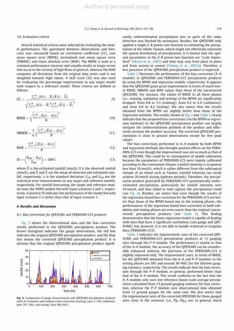
Fig. 3 shows the observational data and the bias correctionresults performed in the QPESUMS precipitation product. Thebrown histogram indicates the gauge observations, the red lineindicates the original QPESUMS precipitation product, and the blueline means the corrected QPESUMS precipitation product. It isobvious that the original QPESUMS precipitation product signifi-

cantly underestimated precipitation due to parts of the radardetection was blocked by mountains. Besides, the QPESUMS onlyapplied a single Z–R power-law function to estimating the precip-itation of the whole Taiwan, which might not effectively representthe spatial distribution of precipitation. It is known that the opti-mal parameters in the Z–R power-law function are ‘‘scale depen-dent’’ (Morin et al., 2003) and they may vary from place to placeand from season to season (Chiang et al., 2007a). Therefore, alow precision of the QPESUMS precipitation product is expected.

Table 2 illustrates the performance of the bias correction (A–Amodule) in QPESUMS and PERSIANN-CCS precipitation productsby using the BPNN and regression models, respectively. It appearsthat the QPESUMS gains great improvement in terms of much low-er RMSE, NRMSE and MAE values than those of the uncorrectedQPESUMS. For instance, the values of RMSE in all three phases(i.e., training, validation and testing) of the BPNN are significantlydropped: from 8.8 to 3.3 (training); from 6.2 to 2.4 (validation);and from 6.8 to 4.2 (testing). We also notice that the resultsobtained from the BPNN are slightly better than those of theregression methods. The results shown in Fig. 3 and Table 2 clearlyindicate that the proposed bias corrections (via the BPNN or regres-sion methods) in the QPESUMS precipitation product can largelymitigate the underestimation problem of the product and effec-tively increase the product accuracy. The corrected QPESUMS pre-cipitation is close to ground observations except for few peakvalues.

The bias corrections performed in A–A module by both BPNNand regression methods also brought positive effects on the PERSI-ANN-CCS even though the improvement was not as much as that ofthe QPESUMS. This could be in consequence of model calibrationbecause the parameters of PERSIANN-CCS were mainly calibratedaccording to the continental climate (rainfall intensity is in generalless than 10 mm/h), which is rather different from the subtropicalclimate of an island such as Taiwan (rainfall intensity can easilyachieve 20 mm/h during typhoon periods). Therefore, the precipi-tation product generated by PERSIANN-CCS systematically under-estimated precipitation, particularly for rainfall intensity over10 mm/h, and thus failed to well capture the precipitation trend(see Fig. 4). Besides, we notice that even though the results ofthe regression-based bias correction for the PERSIANN-CCS are bet-ter than those of the BPNN-based one in the training phases, theperformances of the regression-based bias correction in both vali-dation and testing phases are even worse than the original (uncor-rected) precipitation products (see Table 2). This findingdemonstrates that the linear regression model is capable of dealingwith data that have a significant correlation (rain gauge and QPE-SUMS), but, however, it is not able to handle scattered or irregulardata (PERSIANN-CCS).

Table 3 indicates the improvement rates of the corrected QPE-SUMS and PERSIANN-CCS precipitation products at 13 gaugingsites through the P–P module. The performance is similar to thatof the A–A module: the accuracy of the QPESUMS can be consider-ably enhanced whereas the precision of the PERSIANN-CCS isslightly improved only. The improvement rates, in terms of RMSE,for the QPESUMS obtained from the A–A and P–P modules in thetesting phases are 38% and around 30–60% (for the thirteen gaug-ing stations), respectively. The results indicate that the bias correc-tion through the P–P module, in general, performed better thanthat of the A–A module. This result conforms to the fact that theA–A module only uses one reference (basin-scale average precipi-tation calculated from 13 ground gauging stations) for bias correc-tion, whereas the P–P module uses observational data obtainedfrom 13 ground gauges for the same task. We also notice thatthe improvement rates of the corrected OPESUMS for those gaugedsites close to the reservoir (i.e., Pg1–Pg4) are, in general, much

0 100 200 300 400 500 600 7000

10

20

30

40

50

time (hr)

rain

fall

(mm

)

gaugewithout correctioncorrected

Fig. 3. Comparison of gauge measurements and QPESUMS precipitation productswith (A–A module) and without a bias correction (training: hour 1–350; validation:hour 351–503; and testing: hour 504–641).



higher than those of the upstream gauged sites (i.e., far from thereservoir, Pg9–Pg13).

After conducting bias corrections, we found that the precision ofthe PERSIANN-CCS was slightly improved only and the improve-ment rates of the OPESUMS in P–P module were larger for gaugesat lower elevations than those at higher elevations. The counter-measures to those phenomena can be further explored in futurework for improving the precision of the remote-sensing precipita-tion products.

4.2. Assimilation of multiple precipitation sources

Even through the bias correction of the PERSIANN-CCS is notsignificant, the PERSIANN-CCS precipitation product may has

potential advantages on data merging because the mechanismsbetween the radar and satellite detection are distinguishing.Besides, the radar coverage could be limited or affected by topog-raphy because the study area belongs to a mountainous watershed.Moreover, the spatial representation of ground gauges is low, and,in particular, no rain gauging station is located above 2000 m in thestudy area. As for satellite images, they are not limited by topogra-phy and are able to provide rapid measurements over large areas.In other words, information comes from satellites may possessimportant precipitation characteristics that may not be capturedby radars or ground gauges. Therefore, the gauge, radar and satel-lite information were taken into consideration for precipitationmerging in this study. Two nonlinear optimization search methods,i.e., the GA and the least square method (LSM), were conducted tosearch the optimal merging weighting factors through minimizingEq. (7).

Table 4 shows the optimal merging weighting factors of theassimilated precipitation obtained from the GA and the LSM, inwhich the optimal value of a merging weighting factor representsthe contribution percentage of the corresponding precipitationsource over the assimilated precipitation. Basically, both GA andLSM produced similar results (similar weighting factors and per-formance) under the same conditions. In the present study, theindividual contribution of rain gauge measurements, QPESUMSand PERSIANN-CCS information to the assimilated precipitationsubject to the constraint of h1 + h2 + h3 = 1 was 69–79%, 14–25%and 6–7% accordingly when the A–A module was applied, whereas

Table 2Performance of the bias corrections (A–A module) in QPESUMS and PERSIANN-CCS precipitation products through the BPNN and regression models.

Correction QPESUMS PERSIANN-CCS

Before BPNN Regression Before BPNN Regression

TrainingRMSEa 8.8 3.3 3.4 8.7 8.4 7.1NRMSEa 1.08 0.40 0.42 1.07 1.03 0.87MAEa 5.4 2.0 2.1 5.4 5.2 5.3

ValidationRMSE 6.2 2.4 2.6 6.6 6.5 8.5NRMSE 0.99 0.39 0.43 1.07 1.05 1.37MAE 3.4 1.6 1.6 3.9 3.8 6.5

TestingRMSE 6.8 4.2 4.4 7.2 6.9 7.4NRMSE 1.09 0.67 0.70 1.15 1.11 1.18MAE 4.1 2.4 2.5 4.7 4.8 5.9

a Unit (mm/h).

0 100 200 300 400 500 600 7000

10

20

30

40

50

time (hr)

rain

fall

(mm

)

gaugewithout correctioncorrected

Fig. 4. Comparison of gauge measurements and PERSIANN-CCS precipitationproducts with (A–A module) and without a bias correction (training: hour 1–350;validation: hour 351–503; and testing: hour 504–641).

Table 3Improvement rates of the corrected QPESUMS and PERSIANN-CCS precipitationproducts (P–P module) at 13 rain gauge stations in the testing phase.

RMSE MAE

QPESUMS(%)

PERSIANN-CCS(%)

QPESUMS(%)

PERSIANN-CCS(%)

Pg1 60.3 3.2 60.8 5.1Pg2 52.1 1.9 43.8 1.1Pg3 51.3 0.5 49.5 0.3Pg4 54.1 2.7 52.7 0.9Pg5 30.8 1.5 22.9 0.8Pg6 51.5 2.0 51.9 -0.2Pg7 47.3 0.1 47.5 1.3Pg8 51.7 1.1 52.0 1.0Pg9 43.6 1.8 44.4 0.7Pg10 41.8 2.8 43.6 1.5Pg11 31.8 1.8 37.3 2.3Pg12 44.0 3.3 44.4 1.6Pg13 35.6 1.9 31.8 0.1

Table 4Optimal merging weighting factors for different precipitation products derived fromthe GA and least square method (LSM), and the comparison of ground measurementsand the assimilated precipitation in terms of RMSE.

h1 + h2 + h3 6 1a Module h1 h2 h3 Testing performance(RMSEb)

GA A–A 0.59 0.29 0.06 615P–P 0.56 0.30 0.06 613

LSM A–A 0.56 0.30 0.07 615P–P 0.56 0.30 0.07 613

h1+h2+h3 6 1GA A–A 0.79 0.14 0.07 622

P–P 0.66 0.24 0.10 619LSM A–A 0.69 0.25 0.06 620

P–P 0.69 0.23 0.08 619

a h1, h2, h3 represent the merging weighting factors corresponding to rain gaugemeasurement, corrected radar product and corrected satellite product, respectively.

b Unit (m3/s).



66–69%, 23–24% and 8–10% accordingly when the P–P module wasused. When under the constraint of h1 + h2 + h3 6 1, the optimalweighting factors were more consistent for both A–A and P–P mod-ules no matter which search method was used.

According to the performance obtained from these two types ofconstraints, it shows that a lower RMSE value could be gainedwhen the constraint of h1 + h2 + h3 6 1 was given. We notice thatthe sum of the optimal weighting factors is less than 0.95 for all

cases, which could result in the underestimation of the assimilatedprecipitation. This phenomenon implies an important fact thatnone of these three precipitation sources can observe or detectthe whole rain system or provide sufficient precipitation informa-tion. Even though the assimilated precipitation synthesized in thisstudy produced the minimal simulation errors as compared withany of these precipitation products, some precipitation characteris-tics must have existed, which needs to be explored by specific

0

5

10

15

20

25

30

1 8 15 22 29 36 43 50 57 64 71 78 85 92 99 106 113 120 127 134

Rai

nfal

l (m

m)

Time (hr)

Radar

Satellite

Gauge

Gauge

Assimilation

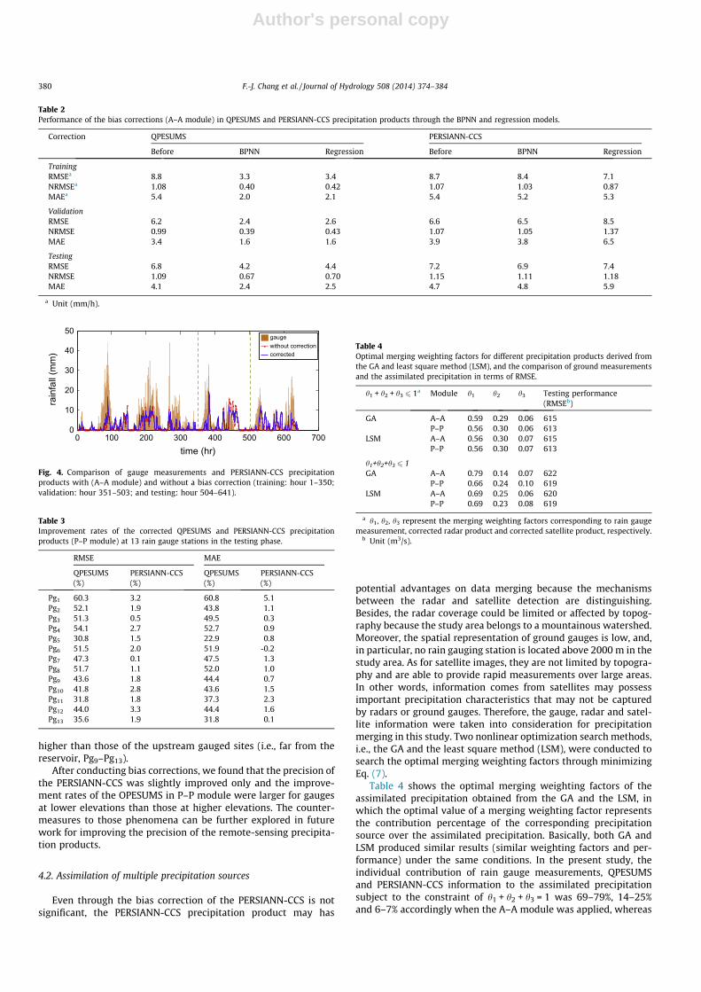
Fig. 5. Contribution of gauge, radar and satellite precipitation products to the assimilated precipitation (A–A module).

Table 5Comparison of rainfall forecasts obtained from the A–A module-based scenarios 1 and 2.

Scenario 1a Scenario 2b

ANFIS ANFIS Regression

Training Validation Testing Training Validation Testing Training Validation Testing

t + 1CC 0.85 0.80 0.71 0.88 0.85 0.85 0.83 0.84 0.83RMSEc 4.33 4.12 4.70 3.88 3.52 3.37 4.55 3.54 3.45MAEc 2.65 2.56 3.07 2.39 2.00 2.23 2.81 2.29 2.36

t + 2CC 0.77 0.74 0.61 0.78 0.79 0.72 0.72 0.74 0.69RMSE 5.21 4.53 5.29 5.05 4.02 4.43 5.67 4.41 4.49MAE 3.32 2.92 3.77 3.14 2.65 3.15 3.63 3.05 3.38

a Inputs: rain gauge, QPESUMS, and PERSIANN-CCS precipitation.b Input: assimilated precipitation.c Unit (mm/h).

0 10 20 30 400

10

20

30

40

observation (mm)

pred

ictio

n (m

m)

0 10 20 30 400

10

20

30

40

observation (mm)

pred

ictio

n (m

m)

(a) one-hour-ahead forecasting (b) two-hour-ahead forecasting

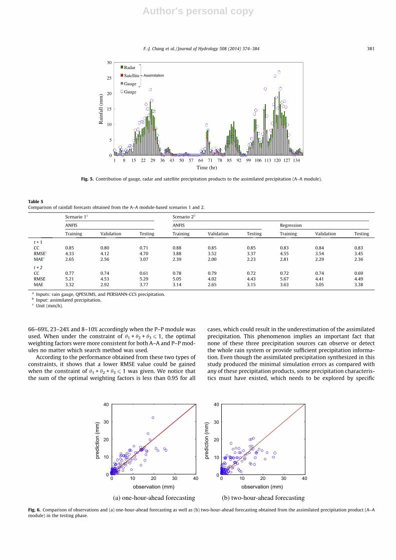
Fig. 6. Comparison of observations and (a) one-hour-ahead forecasting as well as (b) two-hour-ahead forecasting obtained from the assimilated precipitation product (A–Amodule) in the testing phase.



approaches such as the numerical weather analysis. Further inves-tigation of this issue should be another interesting topic and wouldbe of great importance in improving the understanding of real rain-fall system.

Fig. 5 illustrates the comparison of ground measurements (bluecircle) and the assimilated precipitation in A–A module (histo-gram), where the gray, green and red bars individually indicatethe contribution of the gauge measurements, radar and satelliteprecipitation products to the assimilated precipitation, respec-tively. It is clear that both QPESUMS and PERSIANN-CCS informa-tion do participate in the merging process even though theircontributions are relatively low as compared with gauge measure-ments. Besides, the contribution of the PERSIANN-CCS is evenlower than that of the QPESUMS. It might be because the correctedQPESUMS captured precipitation behavior more accurately thanthe corrected PERSIANN-CCS (Figs. 3 and 4). Consequently theimprovement made by the satellite precipitation product is rela-tively limited in this study case.

4.3. Rainfall forecasting by ANFIS models

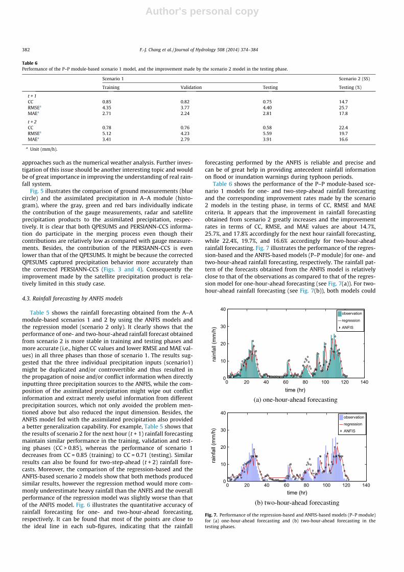
Table 5 shows the rainfall forecasting obtained from the A–Amodule-based scenarios 1 and 2 by using the ANFIS models andthe regression model (scenario 2 only). It clearly shows that theperformance of one- and two-hour-ahead rainfall forecast obtainedfrom scenario 2 is more stable in training and testing phases andmore accurate (i.e., higher CC values and lower RMSE and MAE val-ues) in all three phases than those of scenario 1. The results sug-gested that the three individual precipitation inputs (scenario1)might be duplicated and/or controvertible and thus resulted inthe propagation of noise and/or conflict information when directlyinputting three precipitation sources to the ANFIS, while the com-position of the assimilated precipitation might wipe out conflictinformation and extract merely useful information from differentprecipitation sources, which not only avoided the problem men-tioned above but also reduced the input dimension. Besides, theANFIS model fed with the assimilated precipitation also provideda better generalization capability. For example, Table 5 shows thatthe results of scenario 2 for the next hour (t + 1) rainfall forecastingmaintain similar performance in the training, validation and test-ing phases (CC > 0.85), whereas the performance of scenario 1decreases from CC = 0.85 (training) to CC = 0.71 (testing). Similarresults can also be found for two-step-ahead (t + 2) rainfall fore-casts. Moreover, the comparison of the regression-based and theANFIS-based scenario 2 models show that both methods producedsimilar results, however the regression method would more com-monly underestimate heavy rainfall than the ANFIS and the overallperformance of the regression model was slightly worse than thatof the ANFIS model. Fig. 6 illustrates the quantitative accuracy ofrainfall forecasting for one- and two-hour-ahead forecasting,respectively. It can be found that most of the points are close tothe ideal line in each sub-figures, indicating that the rainfall

forecasting performed by the ANFIS is reliable and precise andcan be of great help in providing antecedent rainfall informationon flood or inundation warnings during typhoon periods.

Table 6 shows the performance of the P–P module-based sce-nario 1 models for one- and two-step-ahead rainfall forecastingand the corresponding improvement rates made by the scenario2 models in the testing phase, in terms of CC, RMSE and MAEcriteria. It appears that the improvement in rainfall forecastingobtained from scenario 2 greatly increases and the improvementrates in terms of CC, RMSE, and MAE values are about 14.7%,25.7%, and 17.8% accordingly for the next hour rainfall forecasting,while 22.4%, 19.7%, and 16.6% accordingly for two-hour-aheadrainfall forecasting. Fig. 7 illustrates the performance of the regres-sion-based and the ANFIS-based models (P–P module) for one- andtwo-hour-ahead rainfall forecasting, respectively. The rainfall pat-tern of the forecasts obtained from the ANFIS model is relativelyclose to that of the observations as compared to that of the regres-sion model for one-hour-ahead forecasting (see Fig. 7(a)). For two-hour-ahead rainfall forecasting (see Fig. 7(b)), both models could

Table 6Performance of the P–P module-based scenario 1 model, and the improvement made by the scenario 2 model in the testing phase.

Scenario 1 Scenario 2 (SS)

Training Validation Testing Testing (%)

t + 1CC 0.85 0.82 0.75 14.7RMSEa 4.35 3.77 4.40 25.7MAEa 2.71 2.24 2.81 17.8

t + 2CC 0.78 0.76 0.58 22.4RMSEa 5.12 4.23 5.59 19.7MAEa 3.41 2.79 3.91 16.6

a Unit (mm/h).

0 20 40 60 80 100 120 1400

10

20

30

40

time (hr)

rain

fall

(mm

/h)

observation

regression

ANFIS

(a) one-hour-ahead forecasting

0 20 40 60 80 100 120 1400

10

20

30

40

time (hr)

rain

fall

(mm

/h)

observation

regression

ANFIS

(b) two-hour-ahead forecasting

Fig. 7. Performance of the regression-based and ANFIS-based models (P–P module)for (a) one-hour-ahead forecasting and (b) two-hour-ahead forecasting in thetesting phases.



still capture the main trend and the variation of observations butthe effect of time-lag occurred. Overall, these results demonstratethat the thirteen rainfall gauging stations indeed contributed themost to the assimilated precipitation while both QPESUMS- andPERSIANN-CCS-derived precipitation products made certain con-tributions to the assimilated precipitation, which shows the effec-tiveness of merging multiple precipitation sources in improvingthe accuracy and reliability of rainfall forecasting.

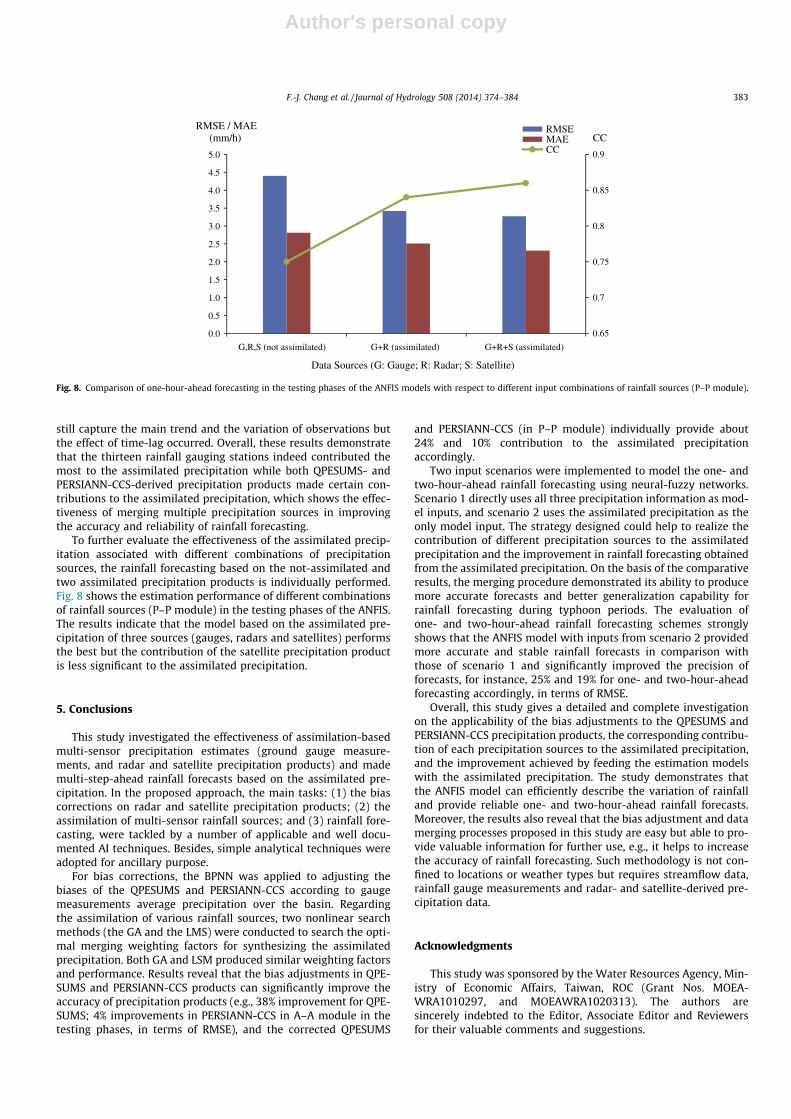
To further evaluate the effectiveness of the assimilated precip-itation associated with different combinations of precipitationsources, the rainfall forecasting based on the not-assimilated andtwo assimilated precipitation products is individually performed.Fig. 8 shows the estimation performance of different combinationsof rainfall sources (P–P module) in the testing phases of the ANFIS.The results indicate that the model based on the assimilated pre-cipitation of three sources (gauges, radars and satellites) performsthe best but the contribution of the satellite precipitation productis less significant to the assimilated precipitation.

5. Conclusions

This study investigated the effectiveness of assimilation-basedmulti-sensor precipitation estimates (ground gauge measure-ments, and radar and satellite precipitation products) and mademulti-step-ahead rainfall forecasts based on the assimilated pre-cipitation. In the proposed approach, the main tasks: (1) the biascorrections on radar and satellite precipitation products; (2) theassimilation of multi-sensor rainfall sources; and (3) rainfall fore-casting, were tackled by a number of applicable and well docu-mented AI techniques. Besides, simple analytical techniques wereadopted for ancillary purpose.

For bias corrections, the BPNN was applied to adjusting thebiases of the QPESUMS and PERSIANN-CCS according to gaugemeasurements average precipitation over the basin. Regardingthe assimilation of various rainfall sources, two nonlinear searchmethods (the GA and the LMS) were conducted to search the opti-mal merging weighting factors for synthesizing the assimilatedprecipitation. Both GA and LSM produced similar weighting factorsand performance. Results reveal that the bias adjustments in QPE-SUMS and PERSIANN-CCS products can significantly improve theaccuracy of precipitation products (e.g., 38% improvement for QPE-SUMS; 4% improvements in PERSIANN-CCS in A–A module in thetesting phases, in terms of RMSE), and the corrected QPESUMS

and PERSIANN-CCS (in P–P module) individually provide about24% and 10% contribution to the assimilated precipitationaccordingly.

Two input scenarios were implemented to model the one- andtwo-hour-ahead rainfall forecasting using neural-fuzzy networks.Scenario 1 directly uses all three precipitation information as mod-el inputs, and scenario 2 uses the assimilated precipitation as theonly model input. The strategy designed could help to realize thecontribution of different precipitation sources to the assimilatedprecipitation and the improvement in rainfall forecasting obtainedfrom the assimilated precipitation. On the basis of the comparativeresults, the merging procedure demonstrated its ability to producemore accurate forecasts and better generalization capability forrainfall forecasting during typhoon periods. The evaluation ofone- and two-hour-ahead rainfall forecasting schemes stronglyshows that the ANFIS model with inputs from scenario 2 providedmore accurate and stable rainfall forecasts in comparison withthose of scenario 1 and significantly improved the precision offorecasts, for instance, 25% and 19% for one- and two-hour-aheadforecasting accordingly, in terms of RMSE.

Overall, this study gives a detailed and complete investigationon the applicability of the bias adjustments to the QPESUMS andPERSIANN-CCS precipitation products, the corresponding contribu-tion of each precipitation sources to the assimilated precipitation,and the improvement achieved by feeding the estimation modelswith the assimilated precipitation. The study demonstrates thatthe ANFIS model can efficiently describe the variation of rainfalland provide reliable one- and two-hour-ahead rainfall forecasts.Moreover, the results also reveal that the bias adjustment and datamerging processes proposed in this study are easy but able to pro-vide valuable information for further use, e.g., it helps to increasethe accuracy of rainfall forecasting. Such methodology is not con-fined to locations or weather types but requires streamflow data,rainfall gauge measurements and radar- and satellite-derived pre-cipitation data.

Acknowledgments

This study was sponsored by the Water Resources Agency, Min-istry of Economic Affairs, Taiwan, ROC (Grant Nos. MOEA-WRA1010297, and MOEAWRA1020313). The authors aresincerely indebted to the Editor, Associate Editor and Reviewersfor their valuable comments and suggestions.

0.65

0.7

0.75

0.8

0.85

0.9

0.0

0.5

1.0

1.5

2.0

2.5

3.0

3.5

4.0

4.5

5.0

G,R,S (not assimilated) G+R (assimilated) G+R+S (assimilated)

CCRMSE / MAE

(mm/h)

Data Sources (G: Gauge; R: Radar; S: Satellite)

RMSEMAECC

Fig. 8. Comparison of one-hour-ahead forecasting in the testing phases of the ANFIS models with respect to different input combinations of rainfall sources (P–P module).



References

Adamowski, J., Chan, H.F., 2011. A wavelet neural network conjunction model forgroundwater level forecasting. Journal of Hydrology 407, 28–40.

Chang, L.C., Chang, F.J., 2001. Intelligent control for modelling of real-time reservoiroperation. Hydrological Processes 15 (9), 1621–1634.

Chang, Y.T., Chang, L.C., Chang, F.J., 2005. Intelligent control for modeling of real-time reservoir operation, Part II: artificial neural network with operating rulecurves. Hydrological Processes 19 (7), 1431–1444.

Chen, C.-Y. et al., 2007. Improving debris flow monitoring in Taiwan by using high-resolution rainfall products from QPESUMS. Natural Hazards 40 (2), 447–461.

Chen, S.T., Yu, P.S., Liu, B.W., 2011. Comparison of neural network architectures andinputs for radar rainfall adjustment for typhoon events. Journal of Hydrology405 (1–2), 150–160.

Chiang, Y.M., Chang, F.J., 2009. Integrating hydrometeorological information forrainfall–runoff modelling by artificial neural networks. Hydrological Processes23 (11), 1650–1659.

Chiang, Y.M., Chang, L.C., Chang, F.J., 2004. Comparison of static-feedforward anddynamic-feedback neural networks for rainfall–runoff modeling. Journal ofHydrology 290 (3–4), 297–311.

Chiang, Y.M., Hsu, K.L., Chang, F.J., Hong, Y., Sorooshian, S., 2007b. Merging multipleprecipitation sources for flash flood forecasting. Journal of Hydrology 340 (3–4),183–196.

Chiang, Y.M., Chang, F.J., Jou, B.J.D., Lin, P.F., 2007a. Dynamic ANN for precipitationestimation and forecasting from radar observations. Journal of Hydrology 334(1–2), 250–261.

Chiang, Y.M., Chang, L.C., Tsai, M.J., Wang, Y.F., Chang, F.J., 2010. Dynamic neuralnetworks for real-time water level predictions of sewerage systems-coveringgauged and ungauged sites. Hydrology and Earth System Sciences 14 (7), 1309–1319.

Chiang, Y.M., Chang, L.C., Tsai, M.J., Wang, Y.F., Chang, F.J., 2011. Auto-control ofpumping operations in sewerage systems by rule-based fuzzy neural networks.Hydrology and Earth System Sciences 15 (1), 185–196.

Chiu, Y.C., Chang, L.C., Chang, F.J., 2007. Using a hybrid genetic algorithm-simulatedannealing algorithm for fuzzy programming of reservoir operation.Hydrological Processes 21 (23), 3162–3172.

Coulibaly, P., Evora, N.D., 2007. Comparison of neural network methods for infillingmissing daily weather records. Journal of Hydrology 341 (1–2), 27–41.

Firat, M., 2008. Comparison of artificial intelligence techniques for river flowforecasting. Hydrology and Earth System Sciences 12 (1), 123–139.

Grecu, M., Krajewski, W.F., 2000. A large-sample investigation of statisticalprocedures for radar-based short-term quantitative precipitation forecasting.Journal of Hydrology 239 (1–4), 69–84.

Haiden, T. et al., 2011. The Integrated Nowcasting through Comprehensive Analysis(INCA) system and its validation over the eastern Alpine region. Weather andForecasting 26 (2), 166–183.

Haykin, S., 1999. Neural Networks, A Comprehensive Foundation. Prentice Hall,Upper Saddle River.

Hong, Y., Hsu, K.L., Sorooshian, S., Gao, X.G., 2004. Precipitation estimation fromremotely sensed imagery using an artificial neural network cloud classificationsystem. Journal of Applied Meteorology 43 (12), 1834–1852.

Hong, Y., Hsu, K.L., Sorooshian, S., Gao, X.G., 2005. Self-organizing nonlinear output(SONO): a neural network suitable for cloud patch-based rainfall estimation atsmall scales. Water Resources Research 41 (3).

Hong, Y., Chiang, Y.M., Liu, Y., Hsu, K.L., Sorooshian, S., 2006. Satellite-basedprecipitation estimation using watershed segmentation and growinghierarchical self-organizing map. International Journal of Remote Sensing 27(23–24), 5165–5184.

Jang, J.S.R., 1993. Anfis – adaptive-network-based fuzzy inference system. IEEETransactions on Systems Man and Cybernetics 23 (3), 665–685.

Juglea, S., Kerr, Y., Mialon, A., Lopez-Baeza, E., Hsu, K., 2010. Soil moisture modellingof a SMOS pixel: interest of using the PERSIANN database over the ValenciaAnchor Station. Hydrology and Earth System Sciences 14 (8), 1509–1525.

Kidd, C., Kniveton, D.R., Todd, M.C., Bellerby, T.J., 2003. Satellite rainfall estimationusing combined passive microwave and infrared algorithms. Journal ofHydrometeorology 4 (6), 1088–1104.

Kober, K., Craig, G.C., Keil, C., Doernbrack, A., 2012. Blending a probabilisticnowcasting method with a high-resolution numerical weather predictionensemble for convective precipitation forecasts. Quarterly Journal of the RoyalMeteorological Society 138 (664), 755–768.

Kurtulus, B., Razack, M., 2010. Modeling daily discharge responses of a large karsticaquifer using soft computing methods: artificial neural network and neuro-fuzzy. Journal of Hydrology 381 (1–2), 101–111.

Li, M., Shao, Q., 2010. An improved statistical approach to merge satellite rainfallestimates and raingauge data. Journal of Hydrology 385 (1–4), 51–64.

Lohani, A.K., Goel, N.K., Bhatia, K.K.S., 2011. Comparative study of neural network,fuzzy logic and linear transfer function techniques in daily rainfall–runoffmodelling under different input domains. Hydrological Processes 25 (2), 175–193.

Mittermaier, M.P., 2008. Introducing uncertainty of radar-rainfall estimates to theverification of mesoscale model precipitation forecasts. Natural Hazards andEarth System Sciences 8 (3), 445–460.

Morin, E., Krajewski, W.F., Goodrich, D.C., Gao, X., Sorooshian, S., 2003. Estimatingrainfall intensities from weather radar data: the scale-dependency problem.Journal of Hydrometeorology 4 (5), 782–797.

Shu, C., Ouarda, T.B.M.J., 2008. Regional flood frequency analysis at ungauged sitesusing the adaptive neuro-fuzzy inference system. Journal of Hydrology 349 (1–2), 31–43.

Siou, L.K.A., Johannet, A., Borrell, V., Pistre, S., 2011. Complexity selection of a neuralnetwork model for karst flood forecasting: the case of the Lez Basin (southernFrance). Journal of Hydrology 403 (3–4), 367–380.

Sokol, Z., 2006. Nowcasting of 1-h precipitation using radar and NWP data. Journalof Hydrology 328 (1–2), 200–211.

Sokol, Z., Pesice, P., 2012. Nowcasting of precipitation–advective statistical forecastmodel (SAM) for the Czech Republic. Atmospheric Research 103, 70–79.

Yilmaz, A.G., Imteaz, M.A., Jenkins, G., 2011. Catchment flow estimation usingartificial neural networks in the mountainous Euphrates Basin. Journal ofHydrology 410 (1–2), 134–140.

Zahraei, A., Hsu, K.L., Sorooshian, S., Gourley, J.J., Lakshmanan, V., Hong, Y., Bellerby,T., 2012. Quantitative precipitation nowcasting: a Lagrangian pixel-basedapproach. Atmospheric Research 118, 418–434.


Documents

Author's personal copy - CHRSs personal copy Watershed rainfall forecasting using neuro-fuzzy ... Rainfall forecasting Arti cial Neural Network ... commonly coupled with heavy rainfall