Author's personal copys personal copy value ofIi r as a correction to be applied by the user. It is clear that the quality of the dierential ionospheric correc-tion will depend on

This article appeared in a journal published by Elsevier. The attachedcopy is furnished to the author for internal non-commercial researchand education use, including for instruction at the authors institution

and sharing with colleagues.

Other uses, including reproduction and distribution, or selling orlicensing copies, or posting to personal, institutional or third party

websites are prohibited.

In most cases authors are permitted to post their version of thearticle (e.g. in Word or Tex form) to their personal website orinstitutional repository. Authors requiring further information

regarding Elsevier’s archiving and manuscript policies areencouraged to visit:

http://www.elsevier.com/copyright

http://www.elsevier.com/copyright

Author's personal copy

Trans-ionospheric GPS signal delay gradients observed overmid-latitude Europe during the geomagnetic storms of

October–November 2003

S.M. Stankov *, R. Warnant, K. Stegen

Department of Geophysics, Royal Meteorological Institute, B-1180 Brussels, Belgium

Received 21 July 2008; received in revised form 15 December 2008; accepted 16 December 2008

Abstract

Ionospheric disturbances are known to have adverse effects on the satellite-based communication and navigation. One particular typeof ionospheric effects, observed during major geomagnetic storms and threatening the integrity performance of both ground-based andspace-based GNSS augmentation systems, is the sharp increase/decrease in the ionospheric delay that propagates in horizontal direction,thus called for convenience ‘moving ionospheric wall’. This paper presents preliminary results from researching such anomalous iono-spheric delay gradients at European middle latitudes during the storm events of 29 October 2003 and 20 November 2003. For the pur-pose, 30-s GPS data from the Belgian permanent network was used for calculating and analysing the slant ionospheric delay and totalelectron content values. It has been found that, during these two particular storm events, substantial gradients did occur in Europealthough they were not so pronounced as in the American sector.� 2009 Published by Elsevier Ltd on behalf of COSPAR.

Keywords: GNSS; GBAS; SBAS; Aircraft navigation; Ionospheric storm; Ionospheric irregularity

1. Introduction

Satellite navigation uses GNSS (Global NavigationSatellite System) satellite broadcasts to calculate position;however, although possessing many advantages above theconventional navigation aids, the satellite-based navigationis prone to ionospheric effects. When electromagnetic sig-nals traverse the ionosphere, the free electrons cause adelay in comparison to the same signal travelling through‘ionosphere-free’ space. Such a delay induces an error onthe computed position, which error is highly variable, dif-ficult to model, and predict. The differential Global Posi-tioning System (DGPS) approach to correcting for theionospheric delay is based on carrier-smoothed codeobservables and uses a network of fixed, ground-based ref-erence stations to broadcast the difference between the

positions indicated by the satellite systems and the knownfixed positions. The underlying premise is that any tworeceivers that are close together would experience similarerrors. Thus, for a given satellite i and a receiver u, the codemeasurement performed by the user is affected by an iono-spheric error I i

u (also called ionospheric slant delay) whichto a good approximation is given by I i

u ¼ Kf 2 TECi

u. In thisformula, I i

u is the error in metres, K is a constant (equalto 40.3 m3/s2), f is the carrier frequency of the signal (inHz), and TECi

u is the total electron content (TEC), i.e. theintegral of the electron density along the satellite-to-recei-ver ray path. TEC is usually measured in terms of TECunits (TECU), where one TECU corresponds to 1 � 1016

electrons per square metre and, at the GPS L1 frequencyof 1.57542 GHz, is equivalent to a delay of 0.542 ns (i.e.to a path length increase of 0.163 m). Simultaneously, thecode measurement made at a reference station r and thesame satellite i, is affected by an ionospheric error,I i

r ¼ Kf 2 TECi

r. In fact, the reference station provides the

0273-1177/$36.00 � 2009 Published by Elsevier Ltd on behalf of COSPAR.

doi:10.1016/j.asr.2008.12.012

* Corresponding author. Tel.: +32 60 39 54 35; fax: +32 60 39 54 23.E-mail address: [email protected] (S.M. Stankov).

www.elsevier.com/locate/asr

Available online at www.sciencedirect.com

Advances in Space Research 43 (2009) 1314–1324


value of I ir as a correction to be applied by the user. It is

clear that the quality of the differential ionospheric correc-tion will depend on the difference, I i

u � I ir, between the ion-

ospheric slant delays experienced by the user and thereference station (Klobuchar, 1996; Hofmann-Wellenhofet al., 2008). To enhance the quality of the DGPS correc-tion and integrity information, particularly for real-timeapplications such as aircraft navigation, the Ground BasedAugmentation System (GBAS) and the Space Based Aug-mentation System (SBAS) have been developed. Analogueversion of GBAS is the US Local Area Augmentation Sys-tem (LAAS) (Braff, 1998), and similar versions of theSBAS system are the US Wide Area Augmentation System(WAAS) (FAA, 2001), the European Geostationary Navi-gation Overlay Service (EGNOS) (Ventura-Traveset andFlament, 2007), and Japan’s Multi-Functional SatelliteAugmentation System (MSAS).

Many applications (e.g. the aircraft precision verticalguidance), require precise correction and bounding of theionospheric delay errors. The task is complicated by theever-changing ionospheric dynamics, characterized by sub-stantial variations in the vertical and horizontal electrondensity distribution that depends on solar/geomagneticactivity, season and local time (Akasofu and Chapman,1972; Davies, 1990; Hargreaves, 1992). Delays tend to belarger at higher solar activity, larger around the equinoxes,and larger during the day than at night. Additionally,strong ionospheric disturbances, occurring as a result ofsolar events (e.g. solar flares) leading to geomagneticstorms, are capable of inducing large variability in the ion-ospheric delays, thus posing a real threat to aircraft precisepositioning/navigation (Blanch et al., 2001; Luo et al.,2003). Ionospheric storms, and the associated ionosphericspatial and temporal gradients, may also lead to NetworkRTK (Real Time Kinematic) performance degradation(Stankov and Jakowski, 2007). It should be mentioned thathorizontal ionospheric gradients in general are known toaffect other GNSS applications too, these including dual-frequency users where higher-order effects need to be miti-gated in pursue of very high precision (Strangeways, 2000).In the case of LAAS, dual-frequency techniques can deliverrobustness against ionospheric temporal gradients; how-ever, since the raw-code ionospheric delay remains in thesmoothed measurements, large ionospheric spatial gradi-ents still pose a threat (Konno et al., 2006).

Anomalous ionospheric spatial gradients, characterizedwith sharp increase/decrease in ionospheric delays over rel-atively short horizontal distance are of particular concernconsidering their sudden appearance, like a wave with asteep front (or in other popular words, like a moving ‘ion-osphere wall’), their relatively fast propagation and chang-ing behavioural patterns. The concern is due to the worst-case scenarios suggesting that such ‘walls’ might actuallyescape detection and thus cause integrity failures. Forexample, in the case of a GBAS-equipped airport, a situa-tion may occur when the ionospheric wave front may comefrom behind an aircraft (approaching the airport for land-

ing) and overtake this aircraft while also crossing one ormore GPS-to-aircraft signal ray paths. In this way, a differ-ential range error builds up until the wave front passes overthe GBAS ground facility (Luo et al., 2004). Actually, the‘moving ionosphere wall’ phenomenon was originally dis-covered with WAAS post-processed and bias-corrected(a.k.a. ‘supertruth’) data obtained during ionosphericstorms of the recent solar activity maximum (Blanchet al., 2001; Walter et al., 2001; Datta-Barua et al., 2002;Luo et al., 2002, 2003). Exemplary results from the geo-magnetic storm of 6 April 2000 are given in Fig. 1. Similarfeatures were also observed for the storms on 29 October2003 and 20 November 2003 (Dehel et al., 2004). Suchpotentially hazardous ionospheric effects are not yet fullyinvestigated and/or understood.

This paper summarizes our observation of anomalousionospheric delay behaviour in Europe and our prelimin-ary research on the ‘moving ionosphere wall’ phenomenon.Comparisons have been made with corresponding Ameri-can observations during the storms of 29 October and 20November 2003.

2. Case studies

GPS code and phase dual-frequency measurements canbe used to reconstruct the slant TEC in the direction ofall satellites in view from a given GPS station. For the pur-pose of studying ionospheric gradient anomalies, we haveused GPS data, at a 30-s sampling rate, from the Belgianpermanent network of about 70 GNSS stations. However,a smaller selection of stations is used here (Fig. 2, left),namely BRUS (50�470N, 04�210E), DENT (50�560N,03�230E), BREE (51�080N, 05�380E), WARE (50�410N,05�140E), and DOUR (50�050N, 04�350E), chosen becauseof their location and distribution, suitable for researchingthe targeted phenomenon and for adequate comparisonwith the US results. Each station is assigned a unique sym-bol/line which will be used when plotting the measurementsmade at this station. GPS measurements have beenprocessed using a technique developed by Warnant andPottiaux (2000) assuming the standard thin shell model,i.e. the entire ionospheric electron density is assumed con-centrated in a very thin shell at a fixed height (e.g. 350 km).Each ionospheric GPS measurement is represented by alocation in this shell called Ionospheric Piercing Point(IPP) which is the intersection of the GPS signal ray path(from the satellite to the ground reference station) withthe thin shell (Davies, 1990; Leitinger, 1996).

Although data from all the selected stations were pro-cessed and analysed, mostly the measurements from theBREE-WARE-DOUR set of stations is of particular inter-est to us in this study and will be presented in more detail.These three stations were selected because of their geo-graphic locations – optimal distance from one anotherand alignment – suitable for detection of the ionosphericdisturbances and anomalies we are focused on in thispaper. Such selection is well justified, considering the typi-

S.M. Stankov et al. / Advances in Space Research 43 (2009) 1314–1324 1315


cal propagation patterns of ionospheric disturbances dur-ing storms in NNE–SSW direction. To demonstrate thispropagation pattern, the TEC relative deviation from itsmonthly median value is calculated over a grid coveringthe European area. For a given grid point’s location andtime, the relative deviation TECrel (interchangeably, dTEC)is calculated by subtracting the monthly median value,TECmed, from the measured value, TECmes, and dividingthe difference by the TECmed value, i.e. TECrel =(TECmes � TECmed)/TECmed. The median value is com-puted from the sample consisting of the TECmes valuesobtained for the same hour and location within a month-long period centred at this particular time. TECrel is widelyused in the ionospheric research as it enhances the iono-spheric perturbation effects and facilitates the interpreta-tion. For convenience, the TECrel value may be displayedin percentage terms like in the here-provided example ofa typical ionospheric storm development (Fig. 2, right).The observed increase of dTEC between 06:00 and 14:00UT appears first in the northern high latitudes and then

propagates steadily in equatorward direction. The develop-ment and propagation of such an increase is explained withthe action of an eastward directed electric field which pen-etrates from high latitudes toward lower latitudes and thuslifts up the plasma via the electromagnetic (E � B) drifteffect, resulting in a reduced loss rate, that is, in a positivedTEC response (Stankov et al., 2006). In fact, the moving‘ionospheric walls’ detected in the American sector duringthe storms in April 2000, October 2003, and November2003, follow the above-described propagation pattern.

2.1. The ionospheric storm on 29 October 2003

In October 2003 the geomagnetic activity was relativelylow except during the last three days when a large stormtook place. The events at the end of October 2003 werecharacterized by a series of large radiation bursts at theSun and huge coronal mass ejections (CMEs) causingsevere perturbations in the geomagnetic field and in thegeo-plasma environment formed by the magneto- and

Fig. 1. The geomagnetic storm on 6 April 2000. Ionospheric delay gradients (left) moving through multiple sites in the Washington D.C. area (right).(Source: Dehel et al., 2004; US National Geodetic Survey).

Fig. 2. Left: Map of Belgium with the GPS stations used for this study. Right: Maps of the relative TEC deviation (dTEC, in percentage terms) from thecorresponding monthly median values observed during the storm of 24 July 2004. Notice the NNE–SSW propagation pattern of the ionosphericdisturbances.

1316 S.M. Stankov et al. / Advances in Space Research 43 (2009) 1314–1324


ionosphere. On 28 October, while the sunspot group 486faced directly toward Earth, a huge solar flare wasobserved which was the third largest on record since1976. The corresponding CME left the sun at about2000 km/s reaching the Earth magnetosphere in about19 h, around 06:00 UT on 29th October. The subsequentgeomagnetic storm was one of the largest in the past 40years continuing well into 30th and 31st of October. Formost of the time on 29 October the recorded planetary geo-magnetic index Kp was close to its maximum possiblevalue, indicating severe geomagnetic and ionospheric con-ditions (Fig. 4, bottom). Similarly, the other geomagneticindex, Dst, strongly related to the magnetospheric parame-ters, reached values of about �400 nT, thus confirming theextreme intensity and duration of the magnetic storm.These conditions set the background for observing andexperiencing strong ionospheric effects.

During the storm period of 29–31 October 2003,reported were several significant malfunctions due to theadverse effects of the ionosphere perturbations such asinterruption of the WAAS service and degradation ofmid-latitudes GPS reference services. Analyses of thisstorm using stations from the CORS (Continuously Oper-ating Reference Stations) network in USA revealed steepionospheric walls (sharp depletion) (Fig. 3) movingthrough with high speeds and gradients of hundreds ofmm/km (Dehel et al., 2004). A simple way to determinethe direction of the wall movement is by comparing thedelay vs. time profiles from several stations. Thus, thealmost identical profiles at HAG1 and ANP1 suggest thatthe wall passed over those two stations at the same time– in a SW direction perpendicular to the HAG1–ANP1line. The movement is similar to that in the previous caseof 6 April 2000 (Fig. 1) when the pairs WIL1-SHK1,PSU1-RED1, and GAIT-HNPT were consecutively passedover.

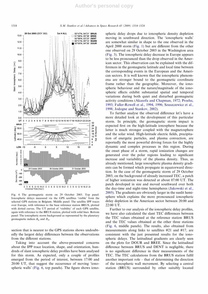
As already stated, it will be interesting to see if similaranomalies are observed here in Europe. For the purpose,we have analysed all available observations carried out atthe selected network of GPS stations in Belgium during thisparticular ionospheric storm. The ionospheric delay mea-surements from 29 October 2003 deduced from all satellite

links on this day are plotted in the top panel of Fig. 4 withreferences to the corresponding ionospheric piercing points(IPP) given in the middle panel. The figure clearly showsthe sharp increase of the ionospheric delay during the mainphase of the storm in the morning hours. This increase issustained well into the afternoon hours in accordance tothe extreme geomagnetic activity conditions. It is followedby a significant drop of the delay in the period between17:00 and 20:00 UT; hence, it is more likely to observeoccurrences of ‘ionospheric walls’ within this time period.

The figure also suggests that a proper detection andanalysis of ‘ionospheric walls’ will have to deal with vari-ous inconveniences, such as the irregular coverage of thesatellite IPP traces, different shape and orientation of thesetraces, short-term visibility of GPS satellites, etc. Themajority of the slant ionospheric delay profiles, obtainedfrom a satellite link, appear in the U-type shapes (Fig. 5,left panel). The ionospheric effects are much smaller whenthe satellite is overhead and become greater and greater asthe satellite nears the horizon because the signal is affectedfor a longer time. Thus, the increases in both ends can beexplained with the effect of the gradually decreasing satel-lite elevation angle (hence increasing slant delay) combinedwith the effect of latitudinal and/or zonal gradients in theionospheric density. Such combination of conditions seri-ously impedes the analysis. In the case presented for satel-lite #5, the IPP traces have relatively small latitudinalresolution and large longitudinal coverage. As a result,what we see is a negligible latitudinal gradient except inthe middle of the time period, i.e. between 13:00 and15:00 UT when the IPPs positions are close to the GPS sta-tions. Obviously, a gradual decrease of the electron densityoccurs in latitude direction, with higher values at the south-ern station DOUR and lower values in the northern sta-tions WARE and BREE. A longitudinal gradient seemsto also occur with higher densities observed in the West.Another frequently observed situation is presented in theright-hand panel of Fig. 5 (satellite #16) when one partof the IPP trace has East–West orientation and the otherone has North–South orientation. Thus, the former partenhances the possible longitudinal gradient and the latterpart enhances the latitudinal gradient. Again, the IPP trace

Fig. 3. The geomagnetic storm on 29 October 2003. Large ionospheric delay gradients (‘ionospheric walls’) (left) observed among CORS clusters in theWashington D.C. area (right). (Source: Dehel et al., 2004; US National Geodetic Survey).



section that is nearest to the GPS stations shows undoubt-edly the largest delay differences between the observationsfrom the different stations.

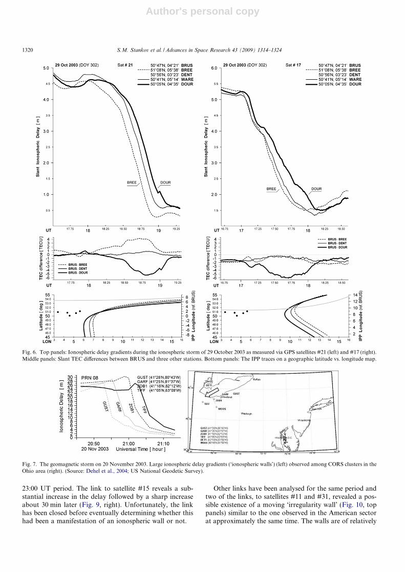
Taking into account the above-presented concernsabout the IPP trace location, shape, and orientation, hun-dreds of slant ionospheric delay profiles have been analysedfor this storm. As expected, only a couple of profilesemerged from the period of interest, between 17:00 and20:00 UT, that suggest the occurrence of moving ‘iono-spheric walls’ (Fig. 6, top panels). The figure shows iono-

spheric delay drops due to ionospheric density depletionmoving in southward direction. The ‘ionospheric walls’are somewhat similar in shape to the one observed in theApril 2000 storm (Fig. 1) but are different from the otherone observed on 29 October 2003 in the Washington area(Fig. 3). The ionospheric delay decrease in Europe appearsto be less pronounced than the drop observed in the Amer-ican sector. This observation can be explained with the dif-ferences in the geomagnetic latitude and local time betweenthe corresponding events in the European and the Ameri-can sectors. It is well known that the ionospheric phenom-ena are stronger bound to the geomagnetic coordinateframe rather than the geographic. Moreover, the iono-spheric behaviour and the nature/magnitude of the iono-spheric effects exhibit substantial spatial and temporalvariations during both quiet and disturbed geomagneticactivity conditions (Akasofu and Chapman, 1972; Proelss,1993; Fuller-Rowell et al., 1994, 1996; Szuszczewicz et al.,1998; Jodogne and Stankov, 2002).

To further analyse the observed difference let’s have amore detailed look at the development of this particularstorm. In principle, the geomagnetic storm impact isexpected first on the high-latitude ionosphere because thelatter is much stronger coupled with the magnetosphereand the solar wind. High-latitude electric fields, precipita-tion of energetic particles, and plasma convection, arereportedly the most powerful driving forces for the highlydynamic and complex processes in this region. Duringthe onset phase of a storm, rapid ionization changes aregenerated over the polar regions leading to significantincrease and variability of the plasma density. Thus, asalready mentioned, large ionospheric plasma density gradi-ents can be formed which propagate in equatorward direc-tion. In the case of the geomagnetic storm of 29 October2003, on the background of already increased TEC, a patchof higher ionization was detected at about 07:00 UT. Thepatch developed in size and moved southward over boththe day-time and night-time hemispheres (Jakowski et al.,2005). The gradients are obviously larger in the sunlit hemi-sphere which explains the more pronounced ionosphericdelay depletion in the American sector between 20:00 and22:00 UT.

Further to our analysis of the ionospheric delay profiles,we have also calculated the slant TEC differences betweenthe TEC values obtained at the reference station BRUSand the TEC values obtained at the other three stations(Fig. 6, middle panels). The results, also obtained frommeasurements along links to satellites #21 and #17, areconsistent with the just presented results for the iono-spheric delays. The latitudinal gradients are clearly seenon the plots for DOUR and BREE. Since the latitudinaldifference between BRUS and DENT is negligible, thereis no significant difference in their measurements of theTEC. The TEC calculations from the BRUS station fulfilanother important role – that of determining the directionof the ionospheric wall movement. By selecting a centralstation (BRUS) surrounded by other suitably located

Fig. 4. The geomagnetic storm on 29 October 2003. Top panel:Ionospheric delays measured via the GPS satellites ‘visible’ from theselected GPS stations in Belgium. Middle panel: The satellite IPP tracesover Europe, with reference to the base reference station BRUS, plottedwith dotted curves. The UT period of ‘visibility’ of each GPS satellite,again with reference to the BRUS station, plotted with solid lines. Bottompanel: The ionospheric storm background as represented by the planetarygeomagnetic indices Kp and Dst.



stations in all possible directions, a star-like formation isset that can help to estimate, to a great level of precision,the direction of the ionospheric gradients propagation.For example one can easily distinguish the almost flat curverepresenting the BRUS-DENT difference from the oppo-sitely varying BRUS-BREE and BRUS-DOUR differences(Fig. 6, middle left panel).

2.2. The ionospheric storm on 20 November 2003

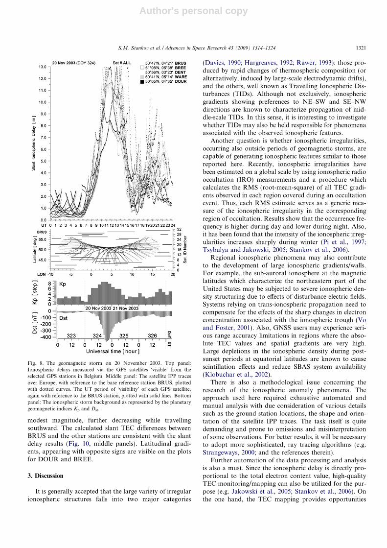
A full halo coronal mass ejection (CME) associated witha relatively moderate, M-class, solar flare started on 18November 2003. The CME, accompanied by a high-speed(about 700 km/s) solar wind and a strong southward com-ponent (about 60 nT at 1 AU) of the interplanetary mag-netic field (IMF), reached the Earth’s magnetosphere on20 November 2003, thus inducing the most intense geo-magnetic storm of the current solar cycle. The geomagneticstorm commenced at 08:03 UT and by 20:00 UT the Dst

index reached the �472 nT mark (Fig. 8, bottom panels).As during the previous storm of 29 October, large iono-

spheric gradients (‘ionospheric walls’) (Fig. 7, left panel)were observed among CORS clusters in the Ohio area(right panel) on 20 November 2003. The ionospheric gradi-ent is shown crossing the station GUST, then GARF,ZOB1, then TIFF (Fig. 7, right panel). The GARF toZOB1 gradient was estimated to be about 20 m in 50 km

distance (i.e. 400 mm/km) and the speed of the wall wasestimated at about 250 m/s (Dehel et al., 2004).

Again, similarly to the case of the 29 October 2003storm, the available GPS observations from 20 November2003 have been analysed. The ionospheric delay measure-ments deduced from all satellite links on this day are plot-ted in the upper panel of Fig. 8, again with references to thecorresponding ionospheric piercing points given in the bot-tom panel. The figure clearly shows the sharp increase ofthe ionospheric delay soon after the onset of the storm fol-lowed by a sharp decrease during the ‘negative phase’ ofthe storm. Very interesting is the period of major perturba-tions of the delay in the evening period between 17:00 and23:00 UT. We will turn our attention to this particular per-iod with the purpose of finding steep ionospheric density/delay gradients.

Again, the task is complicated due to the great variabil-ity in satellite IPP trace shapes and orientations (Fig. 9,left). Although the decrease of the ionospheric delay inthe afternoon hour is clearly visible, the magnitude of thedecrease and the speed of this decrease vary significantlyfrom link to link. Notice how, despite the time coincidenceof satellite visibility, the measurements along the link tosatellite #30 deviate significantly from the measurementsbased on other satellite links. It confirms again the impor-tance of proper consideration of the IPP trace characteris-tics. As mentioned above, the attention is on the 17:00 to

Fig. 5. Top panels: Ionospheric delays during the storm of 29 October 2003 as measured via GPS satellites #5 (left) and #16 (right). Bottom panels: Thesatellite IPP traces on a geographic latitude vs. longitude map. The longitudinal excursion of the satellite IPP (ref. station BRUS) during the selected UTperiod is plotted with a solid line.



23:00 UT period. The link to satellite #15 reveals a sub-stantial increase in the delay followed by a sharp increaseabout 30 min later (Fig. 9, right). Unfortunately, the linkhas been closed before eventually determining whether thishad been a manifestation of an ionospheric wall or not.

Other links have been analysed for the same period andtwo of the links, to satellites #11 and #31, revealed a pos-sible existence of a moving ‘irregularity wall’ (Fig. 10, toppanels) similar to the one observed in the American sectorat approximately the same time. The walls are of relatively

Fig. 6. Top panels: Ionospheric delay gradients during the ionospheric storm of 29 October 2003 as measured via GPS satellites #21 (left) and #17 (right).Middle panels: Slant TEC differences between BRUS and three other stations. Bottom panels: The IPP traces on a geographic latitude vs. longitude map.

Fig. 7. The geomagnetic storm on 20 November 2003. Large ionospheric delay gradients (‘ionospheric walls’) (left) observed among CORS clusters in theOhio area (right). (Source: Dehel et al., 2004; US National Geodetic Survey).



modest magnitude, further decreasing while travellingsouthward. The calculated slant TEC differences betweenBRUS and the other stations are consistent with the slantdelay results (Fig. 10, middle panels). Latitudinal gradi-ents, appearing with opposite signs are visible on the plotsfor DOUR and BREE.

3. Discussion

It is generally accepted that the large variety of irregularionospheric structures falls into two major categories

(Davies, 1990; Hargreaves, 1992; Rawer, 1993): those pro-duced by rapid changes of thermospheric composition (oralternatively, induced by large-scale electrodynamic drifts),and the others, well known as Travelling Ionospheric Dis-turbances (TIDs). Although not exclusively, ionosphericgradients showing preferences to NE–SW and SE–NWdirections are known to characterize propagation of mid-dle-scale TIDs. In this sense, it is interesting to investigatewhether TIDs may also be held responsible for phenomenaassociated with the observed ionospheric features.

Another question is whether ionospheric irregularities,occurring also outside periods of geomagnetic storms, arecapable of generating ionospheric features similar to thosereported here. Recently, ionospheric irregularities havebeen estimated on a global scale by using ionospheric radiooccultation (IRO) measurements and a procedure whichcalculates the RMS (root-mean-square) of all TEC gradi-ents observed in each region covered during an occultationevent. Thus, each RMS estimate serves as a generic mea-sure of the ionospheric irregularity in the correspondingregion of occultation. Results show that the occurrence fre-quency is higher during day and lower during night. Also,it has been found that the intensity of the ionospheric irreg-ularities increases sharply during winter (Pi et al., 1997;Tsybulya and Jakowski, 2005; Stankov et al., 2006).

Regional ionospheric phenomena may also contributeto the development of large ionospheric gradients/walls.For example, the sub-auroral ionosphere at the magneticlatitudes which characterize the northeastern part of theUnited States may be subjected to severe ionospheric den-sity structuring due to effects of disturbance electric fields.Systems relying on trans-ionospheric propagation need tocompensate for the effects of the sharp changes in electronconcentration associated with the ionospheric trough (Voand Foster, 2001). Also, GNSS users may experience seri-ous range accuracy limitations in regions where the abso-lute TEC values and spatial gradients are very high.Large depletions in the ionospheric density during post-sunset periods at equatorial latitudes are known to causescintillation effects and reduce SBAS system availability(Klobuchar et al., 2002).

There is also a methodological issue concerning theresearch of the ionospheric anomaly phenomena. Theapproach used here required exhaustive automated andmanual analysis with due consideration of various detailssuch as the ground station locations, the shape and orien-tation of the satellite IPP traces. The task itself is quitedemanding and prone to omissions and misinterpretationof some observations. For better results, it will be necessaryto adopt more sophisticated, ray tracing algorithms (e.g.Strangeways, 2000; and the references therein).

Further automation of the data processing and analysisis also a must. Since the ionospheric delay is directly pro-portional to the total electron content value, high-qualityTEC monitoring/mapping can also be utilized for the pur-pose (e.g. Jakowski et al., 2005; Stankov et al., 2006). Onthe one hand, the TEC mapping provides opportunities

Fig. 8. The geomagnetic storm on 20 November 2003. Top panel:Ionospheric delays measured via the GPS satellites ‘visible’ from theselected GPS stations in Belgium. Middle panel: The satellite IPP tracesover Europe, with reference to the base reference station BRUS, plottedwith dotted curves. The UT period of ‘visibility’ of each GPS satellite,again with reference to the BRUS station, plotted with solid lines. Bottompanel: The ionospheric storm background as represented by the planetarygeomagnetic indices Kp and Dst.



for covering larger areas thus allowing for easier detectionand analysis of dynamic ionospheric structures. On theother hand, since TEC values at grid points are mostlyobtained by interpolating between measured values, TECgradients obtained in this way may smooth out the realgradients and thus deem the interpretation incorrect.Therefore, the TEC mapping should be made with a veryhigh spatial and temporal resolution, and for aircraft nav-igation purposes, it should be provided in real time. Real-time reconstruction of the vertical ionospheric density dis-tribution via simultaneous GNSS and digital ionosondemeasurements (Stankov et al., 2003, 2005), can also be uti-lized, e.g. for map verification purposes or for ionosphericslab thickness estimation. The latter can provide valuableclues about the local depth of the ionosphere that may inturn help the estimation of the maximum ionospheric delayand the ionospheric threat modelling in general (Blanchet al., 2001). Short-term forecasting of the ionosphericparameters (e.g. Houminer and Soicher, 1996; Muhtarovand Kutiev, 1999; Stankov et al., 2004) is also a key instru-ment in the ionospheric effects mitigation.

It is therefore expected that the combined use of diverseobservation techniques and the utilization of complexmonitoring/modelling approaches would bring more reli-

able results in mitigating the effects of the ionosphericgradients.

4. Conclusions

TEC and ionospheric delay measurements, performedin Belgium during the geomagnetic storms of 29 October2003 and 20 November 2003, have been analysed insearch of anomalous moving ionospheric walls similarto those reported for the United States. It has beenfound that such similar ionospheric delay gradients didoccur in Europe during these storms, although they werenot so pronounced as in the American sector. Furtherresearch is needed, with available data from other geo-magnetic storm events, in order to analyse this interest-ing phenomenon. In particular, it remains to beinvestigated whether ionospheric effects of such scale/nat-ure are due to concrete ionospheric conditions that devel-oped during these events only or, in general, the localionosphere conditions in US are more susceptible to suchphenomena. In this sense, one important objective shouldbe to assess the integrity risk to GBAS/SBAS servicesand thus to determine if additional protection is neededfor GNSS-based aircraft navigation in Europe.

Fig. 9. Top panels: Ionospheric delays during the storm of 20 November 2003 as measured via GPS satellite selection 3 (#06, #17, #24, #25, #30) (left)and satellite #15 (right). Bottom left panel: The satellite IPP traces with reference to the base reference station BRUS, plotted with dotted curves and thecorresponding UT periods of GPS ‘visibility’ plotted with solid lines. Bottom right panel: The satellite IPP traces on a geographic latitude vs. longitudemap (right).



Acknowledgements

This research is supported by the Royal MeteorologicalInstitute of Belgium via Grant GJU/06/2423/CTR/GALO-CAD and the RMI Centre of Excellence.

References

Akasofu, S.I., Chapman, S. Solar-Terrestrial Physics. Oxford UniversityPress, Oxford, UK, 901 pp., 1972.

Blanch, J., Walter, T., Enge, P. Ionospheric threat model methodology forWAAS, in: Proceedings of the ION Annual Meeting, June 2001,Albuquerque, NM, pp. 508–513, 2001.

Braff, R. Description of the FAA’s Local Area Augmentation System(LAAS). J. Inst. Navigation 44 (4), 411–424 (Winter 1997–1998), 1998.

Datta-Barua, S., Walter, T., Pullen, S., Luo, M., Blanch, J., Enge, P.Using WAAS ionospheric data to estimate LAAS short baselinegradients, in: Proceedings of the ION National Technical Meeting,January 28–30, 2002, San Diego, CA, pp. 523–531, 2002.

Davies, K. Ionospheric Radio. Peter Peregrinus Ltd., London, UK, 1990.

Dehel, T., Lorge, F., Warburton, J., Nelthropp, D. Satellite navigation vs.the ionosphere: where are we, and where are we going? in: Proceedingsof the ION GNSS, September 21–24, 2004, Long Beach, CA, pp. 375–386, 2004.

Federal Aviation Administration (FAA). Specification for the Wide AreaAugmentation System (WAAS). Document DTFA01-96-C-00025Modification No. 0111/FAA-E- 2892b Change 2 (August 13, 2001),US Department of Transportation, 2001.

Fuller-Rowell, T.J., Codrescu, M.V., Moffett, R.J., Quegan, S. Responseof the thermosphere and ionosphere to geomagnetic storms. J.Geophys. Res. 99 (3), 3893–3914, 1994.

Fuller-Rowell, T.J., Codrescu, M.V., Rishbeth, H., Moffett, R.J., Quegan,S. On the seasonal response of the thermosphere and ionosphere togeomagnetic storms. J. Geophys. Res. 101 (2), 2343–2353, 1996.

Hargreaves, J.K. The Solar-Terrestrial Environment. Cambridge Univer-sity Press, Cambridge, 1992.

Hofmann-Wellenhof, B., Lichtenegger, H., Wasle, E. GNSS – GlobalNavigation Satellite Systems: GPS, GLONASS & More. Springer,Vienna, New York, 516 pp., 2008.

Houminer, Z., Soicher, H. Improved short-term predictions of foF2

using GPS time delay measurements. Radio Sci. 31 (5), 1099–1108,1996.

Fig. 10. Top panels: Ionospheric delay gradients during the ionospheric storm of 20 November 2003 as measured via GPS satellites #11 (left) and #31 (right).Middle panels: Slant TEC differences between BRUS and three other stations. Bottom panels: The IPP traces on a geographic latitude vs. longitude map.



Jakowski, N., Stankov, S.M., Klaehn, D. Operational space weatherservice for GNSS precise positioning. Ann. Geophys. 23 (9), 3071–3079, 2005.

Jodogne, J.C., Stankov, S.M. Ionosphere–plasmasphere response togeomagnetic storms studied with the RMI-Dourbes comprehensivedatabase. Ann. Geophys. 45 (5), 629–647, 2002.

Klobuchar, J.A. Ionospheric effects on GPS, in: Parkinson, B.W., Spilker,J.J. Jr. (Eds.), Global Positioning System: Theory and Application,vol. 164. American Institute of Aeronautics and Astronautics, Wash-ington, DC, pp. 485–515, 1996.

Klobuchar, J.A., Doherty, P., El-Arini, M.B., Lejeune, R., Dehel, T. Totalelectron content effects on GNSS augmentation system, in: Proceed-ings of the XXVIIth URSI General Assembly, Maastricht, 2002.

Konno, H., Pullen, S., Rife, J., Enge, P. Evaluation of two types of dual-frequency differential GPS techniques under anomalous ionosphereconditions, in: Proceedings of the ION National Technical Meeting,January 18–20, 2006, Monterey, CA, vol. 2, pp. 735–747, 2006.

Leitinger, R. Ionospheric electron content, in: Dieminger, W., Hartmann,G.K., Leitinger, R. (Eds.), The Upper Atmosphere – Data Analysisand Interpretation. Springer, Berlin, pp. 660–672, 1996.

Luo, M., Pullen, S., Akos, D., Xie, G., Datta-Barua, S., Walter, T., Enge,P. Assessment of ionospheric impact on LAAS using WAAS super-truth data, in: Proceedings of the ION Annual Meeting, June 24–26,2002, Albuquerque, NM, pp. 175–186, 2002.

Luo, M., Pullen, S., Dennis, J., Konno, H., Xie, G., Walter, T., Enge, P.,Datta-Barua, S., Dehel, T. LAAS ionosphere spatial gradient threatmodel and impact of LGF and airborne monitoring, in: Proceedings ofthe ION GPS, September 9–12, 2003, Portland, OR, pp. 2255–2274,2003.

Luo, M., Pullen, S., Ene, A., Qiu, D., Walter, T., Enge, P. Ionosphericthreat to LAAS: updated model, user impact, and mitigations, in:Proceedings of the ION GNSS, September 21–24, 2004, Long Beach,CA, pp. 2771–2785, 2004.

Muhtarov, P., Kutiev, I. Autocorrelation method for temporal interpo-lation and short-term prediction of ionospheric data. Radio Sci. 34,459–464, 1999.

Pi, X., Mannucci, A.J., Lindqwister, U.J., Ho, C.M. Monitoring of globalionospheric irregularities using the worldwide GPS network. Geophys.Res. Lett. 24, 2283, 1997.

Proelss, G.W. On explaining the local time variation of ionospheric stormeffects. Ann. Geophys. 11 (1), 1–9, 1993.

Rawer, K. Wave Propagation in the Ionosphere. Kluwer Academic,Dordrecht, Boston, 486 pp., 1993.

Stankov, S.M., Jakowski, N., Heise, S., Muhtarov, P., Kutiev, I., Kutiev,R. A new method for reconstruction of the vertical electron densitydistribution in the upper ionosphere and plasmasphere. J. Geophys.Res. 108 (A5), 1164, 2003.

Stankov, S.M., Kutiev, I.S., Jakowski, N., Wehrenpfennig, A. GPS TECforecasting based on auto-correlation analysis. Acta Geod. Geophys.Hung. 39 (1), 1–14, 2004.

Stankov, S.M., Jakowski, N., Heise, S. Reconstruction of ion and electrondensity profiles from space-based measurements of the upper electroncontent. Planet. Space Sci. 53 (9), 945–957, 2005.

Stankov, S.M., Jakowski, N., Tsybulya, K., Wilken, V. Monitoring thegeneration and propagation of ionospheric disturbances and effects onGNSS positioning. Radio Sci. 41 (5), RS6S09, 2006.

Stankov, S.M., Jakowski, N. Ionospheric effects on GNSS referencenetwork integrity. J. Atmos. Solar Terr. Phys. 69 (4–5), 485–499,2006.

Strangeways, H.J. Effect of horizontal gradients on ionosphericallyreflected or transionospheric paths using a precise homing-in method.J. Atmos. Solar Terr. Phys. 62 (15), 1361–1376, 2000.

Szuszczewicz, E.P., Lester, M., Wilkinson, P., Blanchard Abdu, M.,Hanbaba, R., Igarashi, K., Pulinets, S., Reddy, B.M. A comparativestudy of global ionospheric responses to intense magnetic stormconditions. J. Geophys. Res. 103 (A6), 11665–11684, 1998.

Tsybulya, K., Jakowski, N. Medium- and small-scale ionospheric irreg-ularities detected by GPS radio occultation method. Geophys. Res.Lett. 32, L09103, 1998.

Ventura-Traveset, J., Flament, D. (Eds.), EGNOS � The EuropeanGeostationary Navigation Overlay System � A Cornerstone ofGalileo. European Space Agency, ESA SP-1303, 2007.

Vo, H.B., Foster, J.C. A quantitative study of ionospheric densitygradients at midlatitudes. J. Geophys. Res. 106 (A10), 21555–21563,2001.

Walter, T., Hansen, A., Blanch, J., Enge, P., Mannucci, A., Pi, X., Sparks,L., Iijima, B., El-Arini, B., Lejeune, R., Hagen, M., Altshuler, E.,Fries, R., Chu, A. Robust detection of ionospheric irregularitiesnavigation. J. Inst. Navigation 48 (2), 89–100, 2001.

Warnant, R., Pottiaux, E. The increase of the ionospheric activityas measured by GPS. Earth Planets Space 52 (11), 1055–1060,2000.


Documents

Author's personal copys personal copy value ofIi r as a correction to be applied by the user. It is clear that the quality of the dierential ionospheric correc-tion will depend on