Author's personal copy - Monash Universityusers.monash.edu.au/~jpwalker/papers/jhydrol14-1.pdf · Author's personal copy Assessing arti cial neural networks and statistical methods

This article appeared in a journal published by Elsevier. The attachedcopy is furnished to the author for internal non-commercial researchand education use, including for instruction at the authors institution

and sharing with colleagues.

Other uses, including reproduction and distribution, or selling orlicensing copies, or posting to personal, institutional or third party

websites are prohibited.

In most cases authors are permitted to post their version of thearticle (e.g. in Word or Tex form) to their personal website orinstitutional repository. Authors requiring further information

regarding Elsevier’s archiving and manuscript policies areencouraged to visit:

http://www.elsevier.com/authorsrights

http://www.elsevier.com/authorsrights

Author's personal copy

Assessing artificial neural networks and statistical methods for infillingmissing soil moisture records

Gift Dumedah ⇑, Jeffrey P. Walker, Li ChikDepartment of Civil Engineering, Monash University, Building 60, Melbourne, 3800 Victoria, Australia

a r t i c l e i n f o

Article history:Received 9 December 2013Received in revised form 4 April 2014Accepted 28 April 2014Available online 9 May 2014This manuscript was handled by AndrasBardossy, Editor-in-Chief, with theassistance of Attilio Castellarin, AssociateEditor

Keywords:Soil moistureTemporal stabilityMissing valuesArtificial neural networksRough sets

s u m m a r y

Soil moisture information is critically important for water management operations including floodforecasting, drought monitoring, and groundwater recharge estimation. While an accurate and continu-ous record of soil moisture is required for these applications, the available soil moisture data, in practice,is typically fraught with missing values. There are a wide range of methods available to infillinghydrologic variables, but a thorough inter-comparison between statistical methods and artificial neuralnetworks has not been made. This study examines 5 statistical methods including monthly averages,weighted Pearson correlation coefficient, a method based on temporal stability of soil moisture, and aweighted merging of the three methods, together with a method based on the concept of rough sets.Additionally, 9 artificial neural networks are examined, broadly categorized into feedforward, dynamic,and radial basis networks. These 14 infilling methods were used to estimate missing soil moisture recordsand subsequently validated against known values for 13 soil moisture monitoring stations for three dif-ferent soil layer depths in the Yanco region in southeast Australia. The evaluation results show that thetop three highest performing methods are the nonlinear autoregressive neural network, rough setsmethod, and monthly replacement. A high estimation accuracy (root mean square error (RMSE) of about0:03 m3=m3) was found in the nonlinear autoregressive network, due to its regression based dynamicnetwork which allows feedback connections through discrete-time estimation. An equally high accuracy(0.05 m3=m3 RMSE) in the rough sets procedure illustrates the important role of temporal persistence ofsoil moisture, with the capability to account for different soil moisture conditions.

Crown Copyright � 2014 Published by Elsevier B.V. All rights reserved.

1. Introduction

Moisture in the upper layers of the soil is a vital component ofthe total water balance in the Earth-atmosphere system, playing acrucial role in several hydrological processes. Soil moisture is oneof the main factors influencing the partitioning of rainfall intoinfiltration and runoff (Mahmood, 1996; Thornthwaite, 1961),controlling the exchange of water and energy between the landsurface and the atmosphere (Legates et al., 2010; Berg andMulroy, 2006; Trenberth and Guillemot, 1998; Houser et al.,1998; Reynolds et al., 2002), and the subsurface water drainagethat influences the leaching of contaminants to groundwater(Langevin and Panday, 2012; Legates et al., 2010). The reliabilityof the above mentioned applications usually depends on theavailability of a continuous time series of soil moisture record.Typically, soil moisture data acquired through ground (or in situ)measurements have missing values due to equipment malfunction,

logger storage overruns, data retrieval problems, and/or severeweather conditions (Dumedah and Coulibaly, 2011; Coulibalyand Evora, 2007). Consequently, the infilling of missing soilmoisture values becomes a necessary procedure to generate a con-tinuous time series record.

Several studies have infilled hydrologic variables includingprecipitation (Mwale et al., 2012; Nkuna and Odiyo, 2011;Coulibaly and Evora, 2007; French et al., 1992; Luck et al.,2000; Abebe et al., 2000; ASCE Task Committee on Applicationof Artificial Neural Networks in Hydrology, 2000b), streamflow(Mwale et al., 2012; Ng and Panu, 2010; Ng et al., 2009;Elshorbagy et al., 2000; ASCE Task Committee on Application ofArtificial Neural Networks in Hydrology, 2000b), evapotranspira-tion (Abudu et al., 2010), air temperature (Coulibaly and Evora,2007; Schneider, 2001), and soil moisture (Gao et al., 2013;Wang et al., 2012; Dumedah and Coulibaly, 2011). The infillingmethods employed in the above studies ranged from statisticalmethods (Gao et al., 2013; Wang et al., 2012; Dumedah andCoulibaly, 2011) to artificial neural networks (Mwale et al.,2012; Nkuna and Odiyo, 2011; Coulibaly and Evora, 2007), with

http://dx.doi.org/10.1016/j.jhydrol.2014.04.0680022-1694/Crown Copyright � 2014 Published by Elsevier B.V. All rights reserved.

⇑ Corresponding author. Tel.: +61 414 273 492.E-mail address: [email protected] (G. Dumedah).

Journal of Hydrology 515 (2014) 330–344

Contents lists available at ScienceDirect

Journal of Hydrology

journal homepage: www.elsevier .com/locate / jhydrol


varying levels of accuracy. While several studies have exploreddifferent infilling approaches, very few studies have beenundertaken to actually reconstruct soil moisture records usingboth statistical and artificial neural network methods. As a result,this study investigates 5 statistical and 9 artificial neural networkmethods, a total of 14 methods to estimate missing soil moisturerecords. The soil moisture monitoring network located in theYanco region of southeast Australia (Smith et al., 2012) is usedas the demonstration data set.

The statistical methods include monthly replacement, weightedPearson correlation, station relative difference, and a weightedmerger of the three statistical methods. Moreover, a method basedon the concept of rough sets (Pawlak, 1997; Pawlak et al., 1995;Pawlak, 1982) was used to determine patterns of temporal stabilityof soil moisture to account for different moisture conditions. Theartificial neural networks (ANNs) evaluated in this stud are broadlycategorized into feedforward group, dynamic group and radialbasis group. Detailed descriptions for the statistical and ANNmethods are provided in the methods section. The selectedapproaches constitute a varied range of methodologies to facilitatea comprehensive inter-comparison between a range of statisticaland ANNs with the potential to identify high performing methodsto infill missing soil moisture. The infilling methods have beenevaluated for their estimation accuracy across 13 soil moisturemonitoring stations independently at three different soil layerdepths in the Yanco area. Moreover, an evaluation of the soilmoisture across the 13 monitoring stations in space and their per-sistence of relative moisture conditions over several time periodswas demonstrated. These space–time distributions are presentedfor the entire period of the chosen soil moisture data, and alsoon a month-by-month basis.

2. Study area and soil moisture data

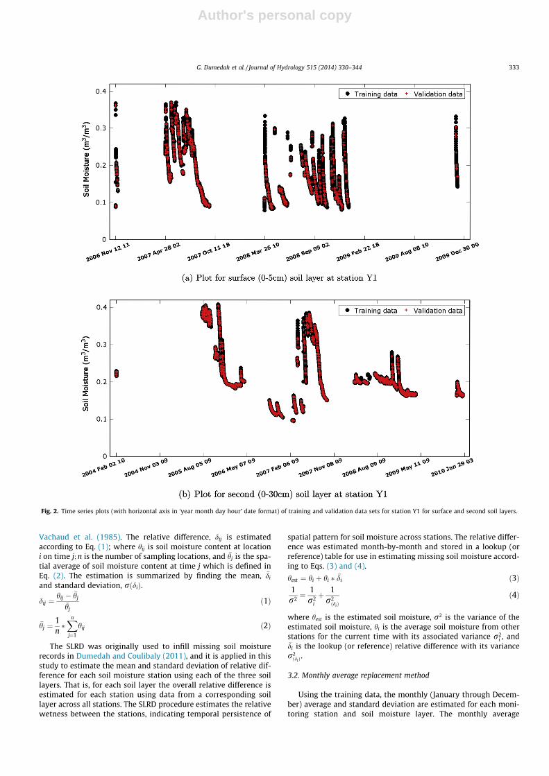
The Yanco area shown in Fig. 1 is a 60 km� 60 km area, locatedin the western plains of the Murrumbidgee Catchment in southeastAustralia where the topography is flat with very few geologicaloutcroppings. Soil texture types are predominantly sandy loams,scattered clays, red brown earths, transitional red brown earth,sands over clay, and deep sands. According to the Digital Atlas ofAustralian Soils, the dominant soil is characterized by plains withdomes, lunettes, and swampy depressions, and divided by contin-uous or discontinuous low river ridges associated with priorstream systems (McKenzie et al., 2000). The area is traversed bypresent stream valleys, layered soil or sedimentary materials com-mon at fairly shallow depths; chief soils are hard alkaline red soils,gray and brown cracking clays.

The Yanco area has 13 soil moisture profile stations which formpart of the OzNet hydrological monitoring network (www.ozne-t.org.au) in the Murrumbidgee Catchment. Generally, profile soilmoisture monitoring at all the stations in the Yanco area have beenin operation since 2004 using Campbell Scientific water contentreflectometers (CS615, CS616) and the Stevens Hydraprobe for foursoil layers: 0–5 cm (or 0–7 cm), 0–30 cm, 30–60 cm and 60–90 cm(Smith et al., 2012). Sensor response to soil moisture varies withsalinity, bulk density, soil type and temperature, so a site-specificsensor calibration has been undertaken using both laboratoryand field measurements for both the reflectometers and theHydraprobes (Western et al., 2000; Western and Seyfried, 2005;Yeoh et al., 2008). As the CS615 and CS616 sensors are particularlysensitive to soil temperature fluctuations (Rüdiger et al., 2010),temperature sensors were installed to provide a continuous recordof soil temperature at the midpoint along the reflectometers.

Fig. 1. Yanco study area in south-east Australia showing the location of soil moisture stations and the soil texture distribution.

G. Dumedah et al. / Journal of Hydrology 515 (2014) 330–344 331


Calibration relationships between the sensor observations, coin-ciding with traditional Time-Domain Reflectometer (TDR)measurements and thermo-gravimetric measurements have beenestablished for both sensors. The average root mean square errorwas found to be 0:03 m3=m3 for both the Campbell Scientific(Yeoh et al., 2008) and Hydraprobe (Merlin et al., 2007) sensors.The soil moisture observations were made at half-hourly timeintervals, but it is noted that the infilling procedure was appliedto an hourly version of the data.

3. Methods for infilling missing soil moisture records

Using the raw soil moisture data, a complete data set wasretrieved by removing all periods with missing records, such thatall soil moisture records were temporally consistent (or common)to all stations for a specific soil layer (Dumedah and Coulibaly,2011; Coulibaly and Evora, 2007). In other words, the completedata set is spatially complete in a way that each record in the dataset at any one station has corresponding records available acrossthe remaining 12 stations for the specified soil layer. As a result,three complete data sets were derived, with each data set corre-sponding to one of the first three soil layer depths. The rationaleto generate the complete data set in this manner is partly becausesoil moisture records are usually missing at the same station for allthree soil depths at any given time period. This approach to gener-ate the complete data record allows the infilling of soil moisture forany soil depth using information from other monitoring stations,when records from other soil depths are often missing. That is,when soil moisture is missing at the one (e.g., surface) soil layerfor any given monitoring station, there is high probability thatthe soil moisture is also missing at the other (e.g., second and third)soil layers for the same station. In practice, it is easier to find dataat other monitoring stations to infill soil moisture for the stationwith the missing record for the specified time period.

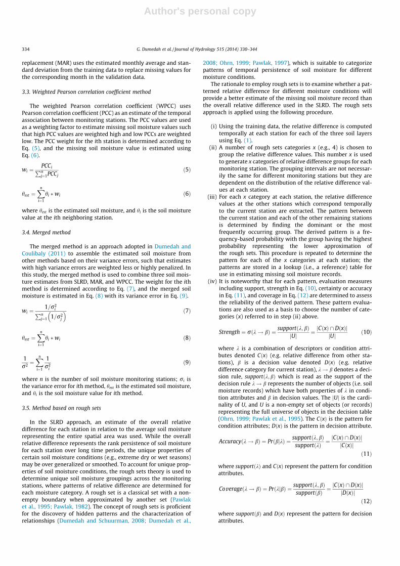
It is noted that soil moisture data from only the first three soillayers are used in this study due to limited records available acrossstations for the 60–90 cm soil layer. The complete data set wasdivided into two: a training data set, and a validation data set.Using the complete data set, 20% of its records were randomlyremoved (temporally and independent of monitoring station) tomakeup the validation data set, with the remaining 80% constitut-ing the training data set for model development. As a result, all theinfilling methods were developed or trained using the training dataset, and subsequently evaluated against known values in the vali-dation data set. The validation data of 20% represents a consider-able proportion of missing soil moisture compared to theproportion of missing values found in past studies, including Gaoet al. (2013); Wang et al. (2012); Dumedah and Coulibaly (2011);and Coulibaly and Evora (2007). The descriptive statistics alongwith the number of records for the training and validation data setsare summarized in Table 1. A time series plot of the training andvalidation data sets for the first and second soil layers at stationY1 is shown in Fig. 2. This plot also illustrates the huge disparitiesin the number of records and the time periods when soil moistureis available between different soil layer depths. It is noted that thenumber of records in the training and validation data sets for spe-cific soil layers is the same across all the monitoring stations, inaccordance with the definition of the complete data. Althoughthe number of records in the validation data set is the same for aspecific soil layer, their time periods are unique as they were ran-domly generated for each station independently. The infillingmethods applied for estimating the missing soil moisture aredescribed in the following sections.

3.1. Station layer relative difference method

The station layer relative difference (SLRD) method is based onthe concept of temporal stability of soil moisture, and usesparametric test of relative difference, which was proposed by

Table 1Number of records, mean and standard deviation of soil moisture (m3=m3) for training and validation data sets for the three soil layers across all 13 soil moisture monitoringstations.

Station Statistic 0–5 cm 0–30 cm 30–60 cm

Training Validation Training Validation Training Validation

1–13 Records 5500 1375 15577 3895 15577 38951 Mean 0.083 0.079 0.146 0.147 0.264 0.263

STD 0.045 0.043 0.036 0.037 0.049 0.0472 Mean 0.184 0.183 0.215 0.215 0.248 0.246

STD 0.068 0.067 0.075 0.077 0.106 0.1043 Mean 0.125 0.127 0.125 0.125 0.153 0.152

STD 0.033 0.033 0.041 0.041 0.042 0.0404 Mean 0.171 0.173 0.272 0.271 0.223 0.223

STD 0.077 0.078 0.091 0.091 0.071 0.0715 Mean 0.147 0.144 0.167 0.166 0.285 0.285

STD 0.066 0.064 0.040 0.039 0.045 0.0456 Mean 0.158 0.154 0.177 0.181 0.269 0.267

STD 0.104 0.105 0.105 0.107 0.080 0.0777 Mean 0.112 0.112 0.187 0.187 0.361 0.361

STD 0.052 0.052 0.064 0.063 0.037 0.0388 Mean 0.101 0.103 0.106 0.106 0.235 0.236

STD 0.073 0.073 0.038 0.038 0.024 0.0259 Mean 0.206 0.202 0.174 0.175 0.377 0.377

STD 0.090 0.090 0.046 0.044 0.057 0.05810 Mean 0.155 0.152 0.221 0.220 0.326 0.327

STD 0.076 0.076 0.102 0.101 0.079 0.08011 Mean 0.113 0.115 0.267 0.269 0.403 0.402

STD 0.073 0.074 0.118 0.119 0.111 0.11112 Mean 0.143 0.145 0.236 0.237 0.337 0.343

STD 0.066 0.066 0.089 0.089 0.091 0.08913 Mean 0.166 0.169 0.206 0.204 0.247 0.247

STD 0.075 0.077 0.107 0.106 0.077 0.075

332 G. Dumedah et al. / Journal of Hydrology 515 (2014) 330–344


Vachaud et al. (1985). The relative difference, dij is estimatedaccording to Eq. (1); where hij is soil moisture content at locationi on time j; n is the number of sampling locations, and �hj is the spa-tial average of soil moisture content at time j which is defined inEq. (2). The estimation is summarized by finding the mean, �di

and standard deviation, rðdiÞ.

dij ¼hij � �hj

�hjð1Þ

�hj ¼1n�Xn

j¼1

hij ð2Þ

The SLRD was originally used to infill missing soil moisturerecords in Dumedah and Coulibaly (2011), and it is applied in thisstudy to estimate the mean and standard deviation of relative dif-ference for each soil moisture station using each of the three soillayers. That is, for each soil layer the overall relative difference isestimated for each station using data from a corresponding soillayer across all stations. The SLRD procedure estimates the relativewetness between the stations, indicating temporal persistence of

spatial pattern for soil moisture across stations. The relative differ-ence was estimated month-by-month and stored in a lookup (orreference) table for use in estimating missing soil moisture accord-ing to Eqs. (3) and (4).

hest ¼ hi þ hi � �di ð3Þ1r2 ¼

1r2

i

þ 1r2ðdiÞ

ð4Þ

where hest is the estimated soil moisture, r2 is the variance of theestimated soil moisture, hi is the average soil moisture from otherstations for the current time with its associated variance r2

i , and�di is the lookup (or reference) relative difference with its variancer2ðdiÞ.

3.2. Monthly average replacement method

Using the training data, the monthly (January through Decem-ber) average and standard deviation are estimated for each moni-toring station and soil moisture layer. The monthly average

Fig. 2. Time series plots (with horizontal axis in ‘year month day hour’ date format) of training and validation data sets for station Y1 for surface and second soil layers.



replacement (MAR) uses the estimated monthly average and stan-dard deviation from the training data to replace missing values forthe corresponding month in the validation data.

3.3. Weighted Pearson correlation coefficient method

The weighted Pearson correlation coefficient (WPCC) usesPearson correlation coefficient (PCC) as an estimate of the temporalassociation between monitoring stations. The PCC values are usedas a weighting factor to estimate missing soil moisture values suchthat high PCC values are weighted high and low PCCs are weightedlow. The PCC weight for the ith station is determined according toEq. (5), and the missing soil moisture value is estimated usingEq. (6).

wi ¼PCCiPnj¼1PCCj

ð5Þ

hest ¼Xn

i¼1

hi �wi ð6Þ

where hest is the estimated soil moisture, and hi is the soil moisturevalue at the ith neighboring station.

3.4. Merged method

The merged method is an approach adopted in Dumedah andCoulibaly (2011) to assemble the estimated soil moisture fromother methods based on their variance errors, such that estimateswith high variance errors are weighted less or highly penalized. Inthis study, the merged method is used to combine three soil mois-ture estimates from SLRD, MAR, and WPCC. The weight for the ithmethod is determined according to Eq. (7), and the merged soilmoisture is estimated in Eq. (8) with its variance error in Eq. (9).

wi ¼1=r2

iPnj¼1 1=r2

j

� � ð7Þ

hest ¼Xn

i¼1

hi �wi ð8Þ

1r2 ¼

Xn

i¼1

1r2

i

ð9Þ

where n is the number of soil moisture monitoring stations; ri isthe variance error for ith method, hest is the estimated soil moisture,and hi is the soil moisture value for ith method.

3.5. Method based on rough sets

In the SLRD approach, an estimate of the overall relativedifference for each station in relation to the average soil moisturerepresenting the entire spatial area was used. While the overallrelative difference represents the rank persistence of soil moisturefor each station over long time periods, the unique properties ofcertain soil moisture conditions (e.g., extreme dry or wet seasons)may be over generalized or smoothed. To account for unique prop-erties of soil moisture conditions, the rough sets theory is used todetermine unique soil moisture groupings across the monitoringstations, where patterns of relative difference are determined foreach moisture category. A rough set is a classical set with a non-empty boundary when approximated by another set (Pawlaket al., 1995; Pawlak, 1982). The concept of rough sets is proficientfor the discovery of hidden patterns and the characterization ofrelationships (Dumedah and Schuurman, 2008; Dumedah et al.,

2008; Ohrn, 1999; Pawlak, 1997), which is suitable to categorizepatterns of temporal persistence of soil moisture for differentmoisture conditions.

The rationale to employ rough sets is to examine whether a pat-terned relative difference for different moisture conditions willprovide a better estimate of the missing soil moisture record thanthe overall relative difference used in the SLRD. The rough setsapproach is applied using the following procedure.

(i) Using the training data, the relative difference is computedtemporally at each station for each of the three soil layersusing Eq. (1).

(ii) A number of rough sets categories x (e.g., 4) is chosen togroup the relative difference values. This number x is usedto generate x categories of relative difference groups for eachmonitoring station. The grouping intervals are not necessar-ily the same for different monitoring stations but they aredependent on the distribution of the relative difference val-ues at each station.

(iii) For each x category at each station, the relative differencevalues at the other stations which correspond temporallyto the current station are extracted. The pattern betweenthe current station and each of the other remaining stationsis determined by finding the dominant or the mostfrequently occurring group. The derived pattern is a fre-quency-based probability with the group having the highestprobability representing the lower approximation ofthe rough sets. This procedure is repeated to determine thepattern for each of the x categories at each station; thepatterns are stored in a lookup (i.e., a reference) table foruse in estimating missing soil moisture records.

(iv) It is noteworthy that for each pattern, evaluation measuresincluding support, strength in Eq. (10), certainty or accuracyin Eq. (11), and coverage in Eq. (12) are determined to assessthe reliability of the derived pattern. These pattern evalua-tions are also used as a basis to choose the number of cate-gories (x) referred to in step (ii) above.

Strength ¼ rðk! bÞ ¼ supportðk; bÞjUj ¼ jCðxÞ \ DðxÞj

jUj ð10Þ

where k is a combination of descriptors or condition attri-butes denoted CðxÞ (e.g. relative difference from other sta-tions), b is a decision value denoted DðxÞ (e.g. relativedifference category for current station), k! b denotes a deci-sion rule, supportðk;bÞ which is read as the support of thedecision rule k! b represents the number of objects (i.e. soilmoisture records) which have both properties of k in condi-tion attributes and b in decision values. The jUj is the cardi-nality of U, and U is a non-empty set of objects (or records)representing the full universe of objects in the decision table(Ohrn, 1999; Pawlak et al., 1995). The CðxÞ is the pattern forcondition attributes; DðxÞ is the pattern in decision attribute.

Accuracyðk! bÞ ¼ PrðbjkÞ ¼ supportðk;bÞsupportðkÞ ¼

jCðxÞ \ DðxÞjjCðxÞj

ð11Þ

where supportðkÞ and CðxÞ represent the pattern for conditionattributes.

Coverageðk! bÞ ¼ PrðkjbÞ ¼ supportðk; bÞsupportðbÞ ¼

jCðxÞ \ DðxÞjjDðxÞj

ð12Þ

where supportðbÞ and DðxÞ represent the pattern for decisionattributes.



(v) To infill a missing record at a monitoring station, the relativedifference is determined for the other monitoring stationswith available soil moisture record for the specified time.The estimated relative difference values are compared tothe lookup (i.e. the reference) patterns to find a matchingcategory for the current station.

(vi) The matching category is then applied to estimate the miss-ing soil moisture record. The rough sets infilling procedure issuch that different (or unique) relative difference values willbe used for the same station depending on the matchingbetween the current pattern and the lookup pattern foundduring the training stage. That is, the rough sets procedureprovides several lookup patterns to account for a specific soilmoisture condition (wet, dry, etc).

3.6. Artificial neural network models

Artificial neural networks have been used to infill hydrologicalvariables including evapotranspiration, precipitation, air tempera-ture, and streamflow (ASCE Task Committee on Application ofArtificial Neural Networks in Hydrology, 2000b). The three broadgroups of ANN which have been widely used in several studies,and used in this study to infill missing soil moisture recordsinclude: feedforward network, dynamic network, and radial basisnetwork. Feedforward neural networks represent nonlinear staticconfigurations with no feedback or delay components such thatthe output is derived from the input through a feedforward con-nection (Beale et al., 2012; Hagan et al., 1996). Dynamic networks,in contrast, use the direct input–output relationships together withfeedbacks from current or previous inputs, outputs, or states of thenetwork (Beale et al., 2012; Coulibaly and Evora, 2007; Haganet al., 1996). Radial basis networks have a similar configurationas feedforward networks but use memory-based learning for theirdesign in a way that learning is viewed as a curve-fitting problemin a high-dimensional space (Beale et al., 2012; ASCE TaskCommittee on Application of Artificial Neural Networks inHydrology, 2000a; Hagan et al., 1996). Radial basis networks spe-cifically have a single hidden layer with linear output layer andare considered local approximations. The individual ANNs arebriefly described below.

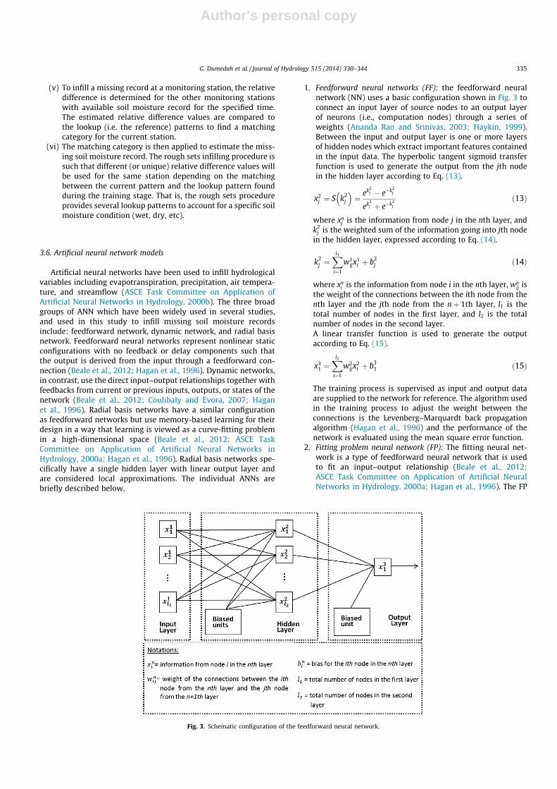
1. Feedforward neural networks (FF): the feedforward neuralnetwork (NN) uses a basic configuration shown in Fig. 3 toconnect an input layer of source nodes to an output layerof neurons (i.e., computation nodes) through a series ofweights (Ananda Rao and Srinivas, 2003; Haykin, 1999).Between the input and output layer is one or more layersof hidden nodes which extract important features containedin the input data. The hyperbolic tangent sigmoid transferfunction is used to generate the output from the jth nodein the hidden layer according to Eq. (13).

x2j ¼ S k2

j

� �¼ ek2

j � e�k2j

ek2j þ e�k2

j

ð13Þ

where xnj is the information from node j in the nth layer, and

k2j is the weighted sum of the information going into jth node

in the hidden layer, expressed according to Eq. (14).

k2j ¼

Xl1

i¼1

w1ijx

1i þ b2

j ð14Þ

where xni is the information from node i in the nth layer, wn

ij isthe weight of the connections between the ith node from thenth layer and the jth node from the nþ 1th layer, l1 is thetotal number of nodes in the first layer, and l2 is the totalnumber of nodes in the second layer.A linear transfer function is used to generate the outputaccording to Eq. (15).

x31 ¼

Xl2

i¼1

w2ijx

2i þ b3

1 ð15Þ

The training process is supervised as input and output dataare supplied to the network for reference. The algorithm usedin the training process to adjust the weight between theconnections is the Levenberg–Marquardt back propagationalgorithm (Hagan et al., 1996) and the performance of thenetwork is evaluated using the mean square error function.

2. Fitting problem neural network (FP): The fitting neural net-work is a type of feedforward neural network that is usedto fit an input–output relationship (Beale et al., 2012;ASCE Task Committee on Application of Artificial NeuralNetworks in Hydrology, 2000a; Hagan et al., 1996). The FP

Fig. 3. Schematic configuration of the feedforward neural network.



establishes a relationship between the station under inves-tigation (output data) and the remaining stations (inputdata). The output layer consists of one node which repre-sents the station under investigation, while the input layercontains 12 nodes, each representing one of the remaining12 stations. The network configuration and the transferfunctions in the hidden and output layer are exactly thesame as the feedforward neural network.

3. Cascade-forward neural networks (CF): The cascade-forwardneural network has a similar configuration as the FF net-work, but includes additional layers to learn complexinput–output relationships more quickly (Beale et al.,2012; Hagan et al., 1996). The additional layers allowweight connection from the input to each layer, and fromeach layer to the successive layers (Omaima AL-Allaf,2012; Beale et al., 2012). The transfer function for the hid-den layer in the FF layout is also used in the CF, but thetransfer function for the output layer is no longer a linearfunction but a hyperbolic tangent sigmoid transfer functionas in the hidden layer.

4. Pattern recognition neural network (PR): The pattern recogni-tion neural network uses the same configuration as the FFnetwork but includes a classification of the input data intospecific classes (ASCE Task Committee on Application ofArtificial Neural Networks in Hydrology, 2000a; Haganet al., 1996). In reference to the FF configuration, the PR usesa hyperbolic tangent sigmoid transfer function for both thehidden and output layer. The hyperbolic tangent sigmoidtransfer function is used in the output layer because theoutput of the function ranges between �1 and +1, for classi-fication of input into different categories.

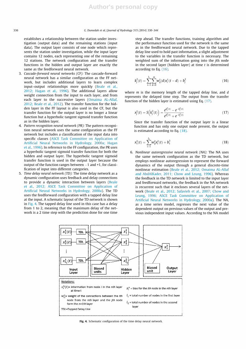
5. Time delay neural network (TD): The time delay network as adynamic configuration uses feedback and delay connectionsto provide a dynamic interaction between layers (Bealeet al., 2012; ASCE Task Committee on Application ofArtificial Neural Networks in Hydrology, 2000a). The TDuses the feedforward configuration with a tapped delay lineat the input. A schematic layout of the TD network is shownin Fig. 4. The tapped delay line used in this case has a delayfrom 1 to 2, meaning that the maximum delay of the net-work is a 2 time step with the prediction done for one time

step ahead. The transfer functions, training algorithm andthe performance function used for the network is the sameas in the feedforward neural network. Due to the tappeddelay line used to hold past information, a slight adjustmentto the variables in the transfer function is necessary. Theweighted sum of the information going into the jth nodein the second layer (hidden layer) at time t is determinedaccording to Eq. (16).

k2j ðtÞ ¼

Xl1

i¼1

Xm

d¼0

w1ijðdÞx1

i ðt � dÞ þ b2j ð16Þ

where m is the memory length of the tapped delay line, and drepresents the delayed time step. The output from the transferfunction of the hidden layer is estimated using Eq. (17).

x2j ðtÞ ¼ S k2

j ðtÞ� �

¼ ek2j ðtÞ � e�k2

j ðtÞ

ek2j ðtÞ þ e�k2

j ðtÞð17Þ

Since the transfer function of the output layer is a linearfunction and has only one output node present, the outputis estimated according to Eq. (18).

x31ðtÞ ¼

Xl2

i¼1

w2ijx

2i ðtÞ þ b3

1 ð18Þ

6. Nonlinear autoregressive neural network (NA): The NA usesthe same network configuration as the TD network, butemploys nonlinear autoregression to represent the forwarddynamics of the output through a general discrete-timenonlinear estimation (Beale et al., 2012; Omaima AL-Allafand AbdAlKader, 2011; Chow and Leung, 1996). Whereasthe feedback in the TD network is limited to the input layerand feedforward networks, the feedback in the NA networkis recurrent such that it encloses several layers of the net-work (Beale et al., 2012; Safavieh et al., 2007; Chow andLeung, 1996; ASCE Task Committee on Application ofArtificial Neural Networks in Hydrology, 2000a). The NA,as a time series model, regresses the next value of thedependent output on previous values of the output and pre-vious independent input values. According to the NA model

Fig. 4. Schematic configuration of the time delay neural network.



defined in Eq. (19), an accurate estimation of the output is afunction of the information on previous values on the out-put variable y and the exogenously determined variable usuch that.

yt ¼ Fðyt�1; yt�2; yt�3; . . . ; yt�Dy;ut ;ut�1;ut�2;ut�3; . . . ;ut�Du Þ

ð19Þ

where yt is the output variable of interest to be predicted, F isthe nonlinear network; and ut is the exogenously determinedinput variable associated with yt . The exogenous inputs,ut; . . . ; ut�Du can be determined with an input delay line withmemory of order Du. Similarly, the endogenous inputs,yt�1; . . . ; yt�Dy

can be estimated with an input delay line withmemory of order Dy. That is, the NA relates the current outputvalue to be estimated with (i) previous values of the outputvariable and (ii) current and previous values of the exogenousinputs.

7. Nonlinear autoregressive neural network with external input(NAE): The NAE has a similar configuration as the NA neuralnetwork, with the same transfer function, training algorithmand performance function (Beale et al., 2012; Omaima AL-Allaf and AbdAlKader, 2011; Chow and Leung, 1996). Whilethe NA does not use exogenous inputs the NAE specificallyemploys the external inputs to estimate the output.

8. Exact radial basis network (RBE): The radial basis neural net-work is a three layer: input, hidden and output network pro-posed by Broomhead and Lowe (1988). The RBE has asimilar configuration as the feedforward network, but itstransfer function in the hidden layer is a radial basis func-tion. The radial basis function estimates the output by usingthe standard Euclidean distance between the input and itscorresponding weight (Beale et al., 2012; ASCE TaskCommittee on Application of Artificial Neural Networks inHydrology, 2000a; Hagan et al., 1996). That is, for each nodethe Euclidean distance between the center and the inputvector is estimated and subsequently transformed by a non-linear function that determines the output of the nodes inthe hidden layer (ASCE Task Committee on Application ofArtificial Neural Networks in Hydrology, 2000a).

9. Generalized regression neural network (GR): The GR networkuses the same network configuration as the radial basislayer but with additional special linear layer. In the GR,the number of nodes can be as many as the number of inputvectors, and nodes weighted input is the standard Euclideandistance between the input vector and its weight vector(Beale et al., 2012).

To allow the network configurations to function at their optimallevel, the number of nodes in each of the layers for all the networkswas determined. Typically, the number of input nodes in the inputlayer is determined by the number of soil moisture monitoring sta-tions available. The NA and NAE neural networks used 13 inputnodes; all the remaining networks used 12 nodes in the inputlayer. The optimal number of nodes in the hidden layer of the neu-ral network is determined using a trial-and-error procedure for allnetworks except the exact radial basis neural network and the gen-eralized regression neural network. The number of nodes testedranged from 2 to 30; the optimal number of nodes and its associ-ated trained network were used to infill the missing soil moisturerecord for subsequent validation period with known data.

4. Results and discussion

The application of the 14 infilling methods is presented in twostages. The first stage illustrates the spatial–temporal variation of

soil moisture for the 13 monitoring stations; whereas the secondstage presents the evaluation of the infilling methods to estimatethe soil moisture records. The infilling methods are evaluated inthree phases: surface soil layer, second soil layer, and the third soillayer independently.

4.1. Space–time variation of station soil moisture

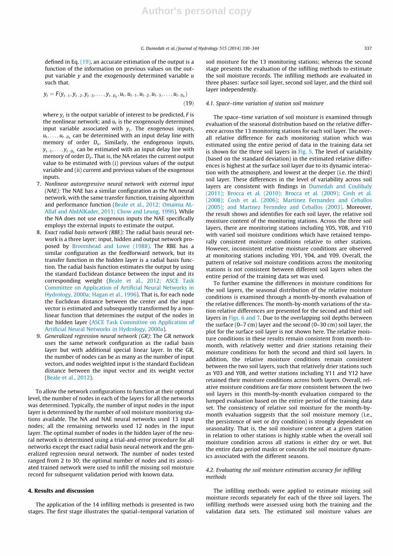
The space–time variation of soil moisture is examined throughevaluation of the seasonal distribution based on the relative differ-ence across the 13 monitoring stations for each soil layer. The over-all relative difference for each monitoring station which wasestimated using the entire period of data in the training data setis shown for the three soil layers in Fig. 5. The level of variability(based on the standard deviation) in the estimated relative differ-ences is highest at the surface soil layer due to its dynamic interac-tion with the atmosphere, and lowest at the deeper (i.e. the third)soil layer. These differences in the level of variability across soillayers are consistent with findings in Dumedah and Coulibaly(2011); Brocca et al. (2010); Brocca et al. (2009); Cosh et al.(2008); Cosh et al. (2006); Martinez Fernandez and Ceballos(2005); and Martnez Fernndez and Ceballos (2003). Moreover,the result shows and identifies for each soil layer, the relative soilmoisture content of the monitoring stations. Across the three soillayers, there are monitoring stations including Y05, Y08, and Y10with varied soil moisture conditions which have retained tempo-rally consistent moisture conditions relative to other stations.However, inconsistent relative moisture conditions are observedat monitoring stations including Y01, Y04, and Y09. Overall, thepattern of relative soil moisture conditions across the monitoringstations is not consistent between different soil layers when theentire period of the training data set was used.

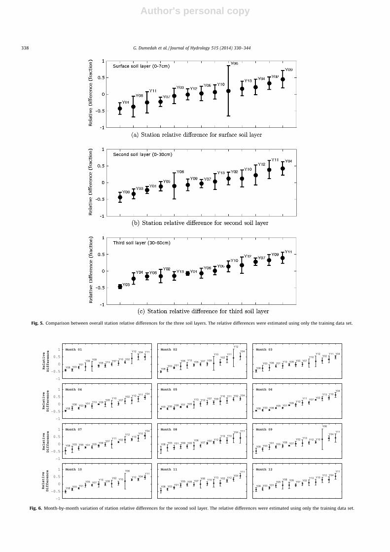
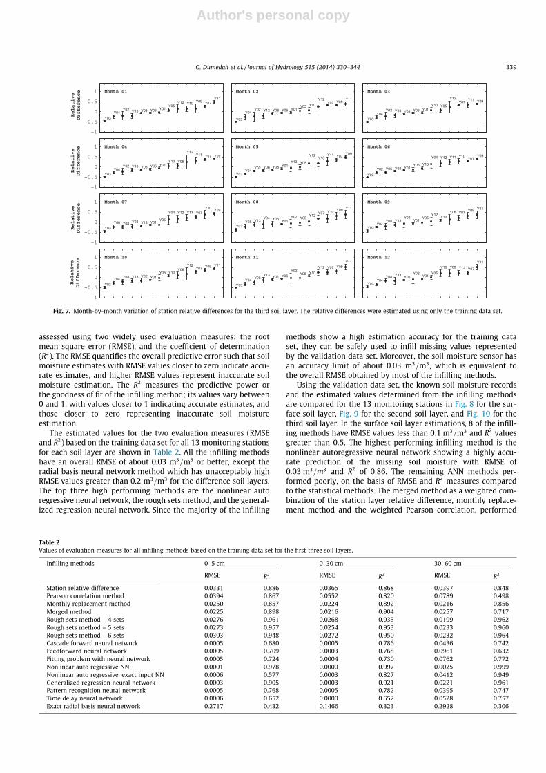
To further examine the differences in moisture conditions forthe soil layers, the seasonal distribution of the relative moistureconditions is examined through a month-by-month evaluation ofthe relative differences. The month-by-month variations of the sta-tion relative differences are presented for the second and third soillayers in Figs. 6 and 7. Due to the overlapping soil depths betweenthe surface (0–7 cm) layer and the second (0–30 cm) soil layer, theplot for the surface soil layer is not shown here. The relative mois-ture conditions in these results remain consistent from month-to-month, with relatively wetter and drier stations retaining theirmoisture conditions for both the second and third soil layers. Inaddition, the relative moisture conditions remain consistentbetween the two soil layers, such that relatively drier stations suchas Y03 and Y08, and wetter stations including Y11 and Y12 haveretained their moisture conditions across both layers. Overall, rel-ative moisture conditions are far more consistent between the twosoil layers in this month-by-month evaluation compared to thelumped evaluation based on the entire period of the training dataset. The consistency of relative soil moisture for the month-by-month evaluation suggests that the soil moisture memory (i.e.,the persistence of wet or dry condition) is strongly dependent onseasonality. That is, the soil moisture content at a given stationin relation to other stations is highly stable when the overall soilmoisture condition across all stations is either dry or wet. Butthe entire data period masks or conceals the soil moisture dynam-ics associated with the different seasons.

4.2. Evaluating the soil moisture estimation accuracy for infillingmethods

The infilling methods were applied to estimate missing soilmoisture records separately for each of the three soil layers. Theinfilling methods were assessed using both the training and thevalidation data sets. The estimated soil moisture values are



Fig. 5. Comparison between overall station relative differences for the three soil layers. The relative differences were estimated using only the training data set.

Fig. 6. Month-by-month variation of station relative differences for the second soil layer. The relative differences were estimated using only the training data set.



assessed using two widely used evaluation measures: the rootmean square error (RMSE), and the coefficient of determination(R2). The RMSE quantifies the overall predictive error such that soilmoisture estimates with RMSE values closer to zero indicate accu-rate estimates, and higher RMSE values represent inaccurate soilmoisture estimation. The R2 measures the predictive power orthe goodness of fit of the infilling method; its values vary between0 and 1, with values closer to 1 indicating accurate estimates, andthose closer to zero representing inaccurate soil moistureestimation.

The estimated values for the two evaluation measures (RMSEand R2) based on the training data set for all 13 monitoring stationsfor each soil layer are shown in Table 2. All the infilling methodshave an overall RMSE of about 0.03 m3=m3 or better, except theradial basis neural network method which has unacceptably highRMSE values greater than 0.2 m3=m3 for the difference soil layers.The top three high performing methods are the nonlinear autoregressive neural network, the rough sets method, and the general-ized regression neural network. Since the majority of the infilling

methods show a high estimation accuracy for the training dataset, they can be safely used to infill missing values representedby the validation data set. Moreover, the soil moisture sensor hasan accuracy limit of about 0.03 m3=m3, which is equivalent tothe overall RMSE obtained by most of the infilling methods.

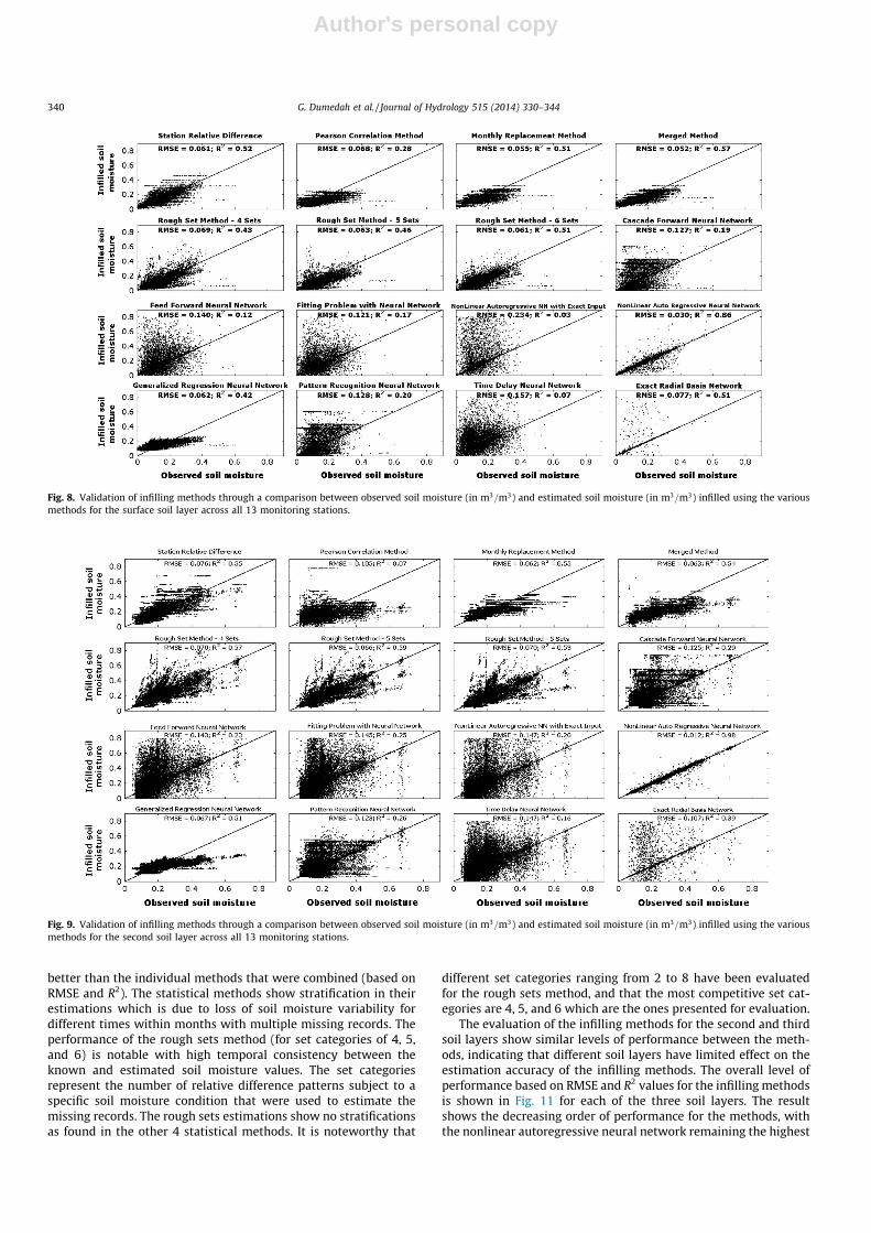
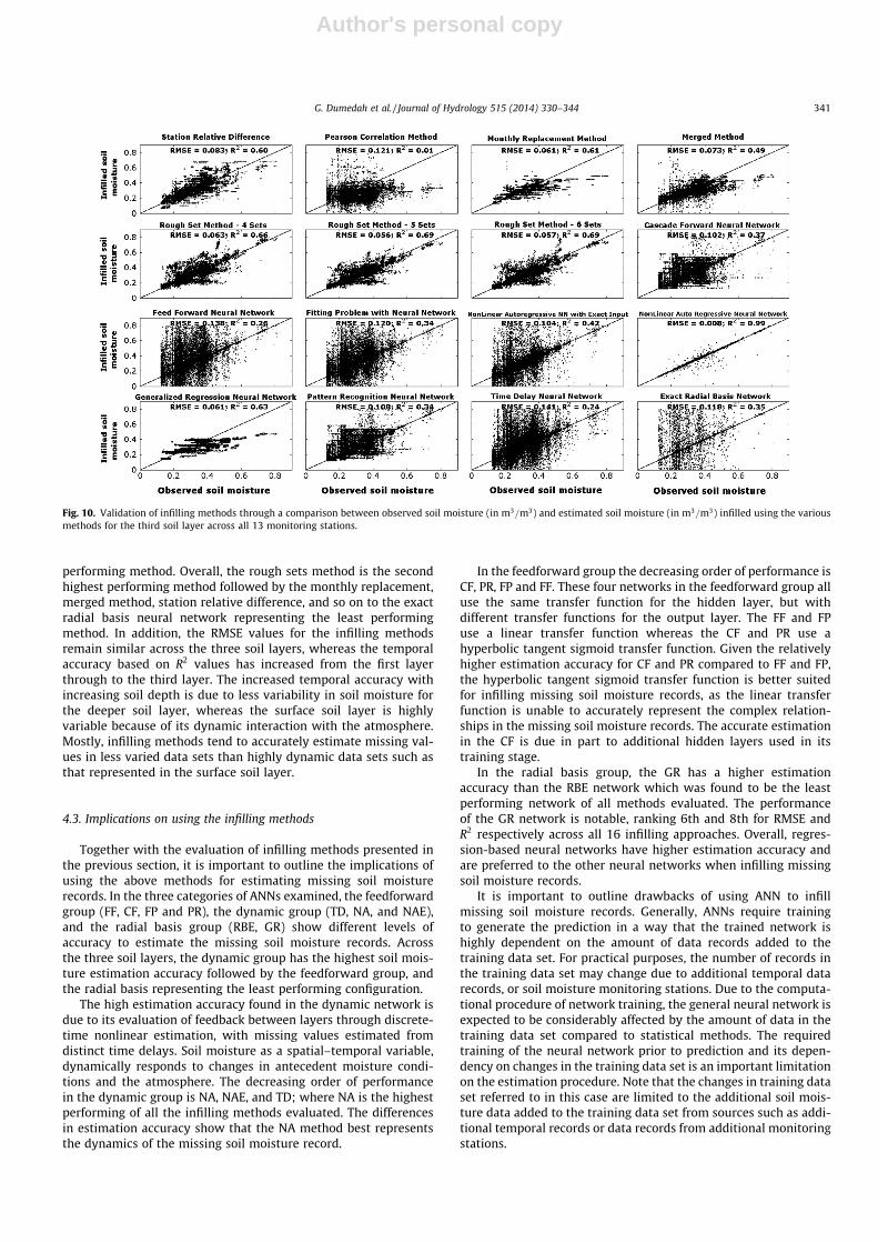
Using the validation data set, the known soil moisture recordsand the estimated values determined from the infilling methodsare compared for the 13 monitoring stations in Fig. 8 for the sur-face soil layer, Fig. 9 for the second soil layer, and Fig. 10 for thethird soil layer. In the surface soil layer estimations, 8 of the infill-ing methods have RMSE values less than 0:1 m3=m3 and R2 valuesgreater than 0:5. The highest performing infilling method is thenonlinear autoregressive neural network showing a highly accu-rate prediction of the missing soil moisture with RMSE of0:03 m3=m3 and R2 of 0:86. The remaining ANN methods per-formed poorly, on the basis of RMSE and R2 measures comparedto the statistical methods. The merged method as a weighted com-bination of the station layer relative difference, monthly replace-ment method and the weighted Pearson correlation, performed

Fig. 7. Month-by-month variation of station relative differences for the third soil layer. The relative differences were estimated using only the training data set.

Table 2Values of evaluation measures for all infilling methods based on the training data set for the first three soil layers.

Infilling methods 0–5 cm 0–30 cm 30–60 cm

RMSE R2 RMSE R2 RMSE R2

Station relative difference 0.0331 0.886 0.0365 0.868 0.0397 0.848Pearson correlation method 0.0394 0.867 0.0552 0.820 0.0789 0.498Monthly replacement method 0.0250 0.857 0.0224 0.892 0.0216 0.856Merged method 0.0225 0.898 0.0216 0.904 0.0257 0.717Rough sets method – 4 sets 0.0276 0.961 0.0268 0.935 0.0199 0.962Rough sets method – 5 sets 0.0273 0.957 0.0254 0.953 0.0233 0.960Rough sets method – 6 sets 0.0303 0.948 0.0272 0.950 0.0232 0.964Cascade forward neural network 0.0005 0.680 0.0005 0.786 0.0436 0.742Feedforward neural network 0.0005 0.709 0.0003 0.768 0.0961 0.632Fitting problem with neural network 0.0005 0.724 0.0004 0.730 0.0762 0.772Nonlinear auto regressive NN 0.0001 0.978 0.0000 0.997 0.0025 0.999Nonlinear auto regressive, exact input NN 0.0006 0.577 0.0003 0.827 0.0412 0.949Generalized regression neural network 0.0003 0.905 0.0003 0.921 0.0221 0.961Pattern recognition neural network 0.0005 0.768 0.0005 0.782 0.0395 0.747Time delay neural network 0.0006 0.652 0.0000 0.652 0.0528 0.757Exact radial basis neural network 0.2717 0.432 0.1466 0.323 0.2928 0.306



better than the individual methods that were combined (based onRMSE and R2). The statistical methods show stratification in theirestimations which is due to loss of soil moisture variability fordifferent times within months with multiple missing records. Theperformance of the rough sets method (for set categories of 4, 5,and 6) is notable with high temporal consistency between theknown and estimated soil moisture values. The set categoriesrepresent the number of relative difference patterns subject to aspecific soil moisture condition that were used to estimate themissing records. The rough sets estimations show no stratificationsas found in the other 4 statistical methods. It is noteworthy that

different set categories ranging from 2 to 8 have been evaluatedfor the rough sets method, and that the most competitive set cat-egories are 4, 5, and 6 which are the ones presented for evaluation.

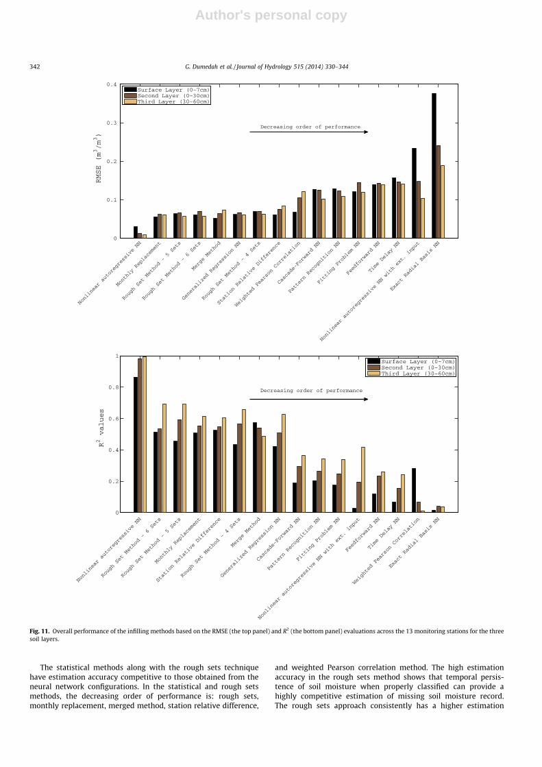
The evaluation of the infilling methods for the second and thirdsoil layers show similar levels of performance between the meth-ods, indicating that different soil layers have limited effect on theestimation accuracy of the infilling methods. The overall level ofperformance based on RMSE and R2 values for the infilling methodsis shown in Fig. 11 for each of the three soil layers. The resultshows the decreasing order of performance for the methods, withthe nonlinear autoregressive neural network remaining the highest

Fig. 8. Validation of infilling methods through a comparison between observed soil moisture (in m3=m3) and estimated soil moisture (in m3=m3) infilled using the variousmethods for the surface soil layer across all 13 monitoring stations.

Fig. 9. Validation of infilling methods through a comparison between observed soil moisture (in m3=m3) and estimated soil moisture (in m3=m3) infilled using the variousmethods for the second soil layer across all 13 monitoring stations.



performing method. Overall, the rough sets method is the secondhighest performing method followed by the monthly replacement,merged method, station relative difference, and so on to the exactradial basis neural network representing the least performingmethod. In addition, the RMSE values for the infilling methodsremain similar across the three soil layers, whereas the temporalaccuracy based on R2 values has increased from the first layerthrough to the third layer. The increased temporal accuracy withincreasing soil depth is due to less variability in soil moisture forthe deeper soil layer, whereas the surface soil layer is highlyvariable because of its dynamic interaction with the atmosphere.Mostly, infilling methods tend to accurately estimate missing val-ues in less varied data sets than highly dynamic data sets such asthat represented in the surface soil layer.

4.3. Implications on using the infilling methods

Together with the evaluation of infilling methods presented inthe previous section, it is important to outline the implications ofusing the above methods for estimating missing soil moisturerecords. In the three categories of ANNs examined, the feedforwardgroup (FF, CF, FP and PR), the dynamic group (TD, NA, and NAE),and the radial basis group (RBE, GR) show different levels ofaccuracy to estimate the missing soil moisture records. Acrossthe three soil layers, the dynamic group has the highest soil mois-ture estimation accuracy followed by the feedforward group, andthe radial basis representing the least performing configuration.

The high estimation accuracy found in the dynamic network isdue to its evaluation of feedback between layers through discrete-time nonlinear estimation, with missing values estimated fromdistinct time delays. Soil moisture as a spatial–temporal variable,dynamically responds to changes in antecedent moisture condi-tions and the atmosphere. The decreasing order of performancein the dynamic group is NA, NAE, and TD; where NA is the highestperforming of all the infilling methods evaluated. The differencesin estimation accuracy show that the NA method best representsthe dynamics of the missing soil moisture record.

In the feedforward group the decreasing order of performance isCF, PR, FP and FF. These four networks in the feedforward group alluse the same transfer function for the hidden layer, but withdifferent transfer functions for the output layer. The FF and FPuse a linear transfer function whereas the CF and PR use ahyperbolic tangent sigmoid transfer function. Given the relativelyhigher estimation accuracy for CF and PR compared to FF and FP,the hyperbolic tangent sigmoid transfer function is better suitedfor infilling missing soil moisture records, as the linear transferfunction is unable to accurately represent the complex relation-ships in the missing soil moisture records. The accurate estimationin the CF is due in part to additional hidden layers used in itstraining stage.

In the radial basis group, the GR has a higher estimationaccuracy than the RBE network which was found to be the leastperforming network of all methods evaluated. The performanceof the GR network is notable, ranking 6th and 8th for RMSE andR2 respectively across all 16 infilling approaches. Overall, regres-sion-based neural networks have higher estimation accuracy andare preferred to the other neural networks when infilling missingsoil moisture records.

It is important to outline drawbacks of using ANN to infillmissing soil moisture records. Generally, ANNs require trainingto generate the prediction in a way that the trained network ishighly dependent on the amount of data records added to thetraining data set. For practical purposes, the number of records inthe training data set may change due to additional temporal datarecords, or soil moisture monitoring stations. Due to the computa-tional procedure of network training, the general neural network isexpected to be considerably affected by the amount of data in thetraining data set compared to statistical methods. The requiredtraining of the neural network prior to prediction and its depen-dency on changes in the training data set is an important limitationon the estimation procedure. Note that the changes in training dataset referred to in this case are limited to the additional soil mois-ture data added to the training data set from sources such as addi-tional temporal records or data records from additional monitoringstations.

Fig. 10. Validation of infilling methods through a comparison between observed soil moisture (in m3=m3) and estimated soil moisture (in m3=m3) infilled using the variousmethods for the third soil layer across all 13 monitoring stations.



The statistical methods along with the rough sets techniquehave estimation accuracy competitive to those obtained from theneural network configurations. In the statistical and rough setsmethods, the decreasing order of performance is: rough sets,monthly replacement, merged method, station relative difference,

and weighted Pearson correlation method. The high estimationaccuracy in the rough sets method shows that temporal persis-tence of soil moisture when properly classified can provide ahighly competitive estimation of missing soil moisture record.The rough sets approach consistently has a higher estimation

Fig. 11. Overall performance of the infilling methods based on the RMSE (the top panel) and R2 (the bottom panel) evaluations across the 13 monitoring stations for the threesoil layers.



accuracy than the station layer relative difference for each of thethree soil layers, meaning that the rough sets grouping whichaccounts for the unique moisture conditions provides a better esti-mation procedure than the lumped station relative differenceacross the entire time period. Specifically, the rough sets methodhas an accuracy increase of 5% in RMSE and 3% in R2 when com-pared to the station relative difference method, thus demonstrat-ing the significance of the rough sets approximation.

5. Conclusions

This study has evaluated 14 infilling methods includingartificial neural network and statistical techniques, to estimatemissing soil moisture records at 13 monitoring stations indepen-dently for three different soil layers. An evaluation of the estimatedsoil moisture values against known records showed that the topthree highest performing methods are the nonlinear autoregressiveneural network, the rough sets method, and the monthly replace-ment. The high estimation accuracy (RMSE of 0.03 m3=m3) foundin the NA network was the result of its regression based dynamicnetwork, which allows feedback connections through discrete-time estimation. Despite the high estimation accuracy of the NAnetwork, the ANNs in general lack a space–time explanation orany insight into the relative soil moisture conditions at the moni-toring stations. Hence, the NA method is best suited for soil mois-ture estimations for cases where the physical space–timerelationships between monitoring stations are not of primaryfocus.

The rough sets approach is advantageous because of its equallyhigh estimation accuracy (RMSE of 0.05 m3=m3) associated with itspattern-based and space–time explanation of relative moistureconditions across monitoring stations. The equally high estimationaccuracy in the rough sets procedure illustrates the important roleof temporal persistence in soil moisture and its grouping toaccount for different soil moisture conditions (e.g. wet, dry, etc).The estimation procedure also illustrates the utility of the roughsets approximation to determine patterns of temporal persistenceof soil moisture that are relevant to different moisture conditions.Consequently, the rough sets method is the preferred approach toextrapolating soil moisture in space and time for other locations,with the capability to account for seasonality. It is noteworthy thatwhile the monthly replacement provides an accurate estimation ofthe missing soil moisture, its infilled values are usually stratifiedinto layers due to multiple missing values in the same month.

The findings from this study point to the potential of thesemethods to infill other hydrologic variables such as air and soiltemperature, precipitation, and evapotranspiration, which are alsoplagued with missing records. Moreover, the findings are directlyapplicable to soil moisture time series data from remote sensing,which can be affected by missing records due to radio frequencyinterference, frozen and ice conditions, problems with retrievalalgorithm convergence, and satellite orbital issues.

Acknowledgements

This work was supported by funding from the AustralianResearch Council (DP0879212). The program for the infilling meth-ods used herein is available upon request from the first author at:[email protected].

References

Abebe, A., Solomatine, D., Venneker, R., 2000. Application of adaptive fuzzy rule –based models for reconstruction of missing precipitation events. Hydrol. Sci. J.45 (3), 425–436.

Abudu, S., Salim Bawazir, A., Phillip King, J., 2010. Infilling missing dailyevapotranspiration data using neural networks. J. Irrig. Drain. Eng. 136 (5),317–325.

Ananda Rao, M., Srinivas, J., 2003. Neural Networks: Algorithms and Applications.Alpha Science International, Pangbourne, ISBN-13: 978-1842651315. p. 239.

ASCE Task Committee on Application of Artificial Neural Networks in Hydrology,2000a. Artificial neural networks in hydrology I: preliminary concepts. J. Hydrol.Eng. 5 (2), 115–123.

ASCE Task Committee on Application of Artificial Neural Networks in Hydrology,2000b. Artificial neural networks in hydrology II: hydrologic applications. J.Hydrol. Eng. 5 (2), 124–137.

Beale, M.H., Hagan, M.T., Demuth, H.B., 2012. Neural Network Toolbox: Users Guide.The MathWorks, Inc.

Berg, A.A., Mulroy, K., 2006. Streamflow predictability given macro-scale estimatesof the initial soil moisture status. Hydrol. Sci. J. 51 (4), 642–654.

Brocca, L., Melone, F., Moramarco, T., Morbidelli, R., 2009. Soil moisture temporalstability over experimental areas in central italy. Geoderma 148, 364–374.

Brocca, L., Melone, F., Moramarco, T., Morbidelli, R., 2010. Spatial–temporalvariability of soil moisture and its estimation across scales. Water Resour.Res. 43, W02516.

Broomhead, D.S., Lowe, D., 1988. Multivariable functional interpolation andadaptive networks. Complex Syst. 2, 321–355.

Chow, T.W.S., Leung, C.T., 1996. Nonlinear autoregressive integrated neural networkdel for short-term load forecasting. IEEE Proc. – Gener., Trans. Distrib 43 (5),500–506.

Cosh, M.H., Jackson, T.J., Starks, P., Heathman, G., 2006. Temporal stability of surfacesoil moisture in the little washita river watershed and its applications insatellite soil moisture product validation. J. Hydrol. 323 (1-4), 168–177.

Cosh, M.H., Jackson, T.J., Moran, S., Bindlish, R., 2008. Temporal persistence andstability of surface soil moisture in a semi – arid watershed. Remote Sens.Environ. 112, 304–313.

Coulibaly, P., Evora, N., 2007. Comparison of neural network methods for infillingmissing daily weather records. J. Hydrol. 341 (1-2), 27–41.

Dumedah, G., Coulibaly, P., 2011. Evaluation of statistical methods for infillingmissing values in high-resolution soil moisture data. J. Hydrol. 400 (1-2), 95102.http://dx.doi.org/10.1016/j.jhydrol.2011.01.028.

Dumedah, G., Schuurman, N., 2008. Minimizing the effects of inaccurate sedimentdescription in borehole data using rough set theory and transition probability. J.Geogr. Syst. 10 (3), 291–315.

Dumedah, G., Schuurman, N., Yang, W., 2008. Minimizing effects of scale distortionfor spatially grouped census data using rough sets. J. Geogr. Syst. 10 (1), 47–69.

Elshorbagy, A.A., Panu, U.S., Simonovic, S.P., 2000. Group – based estimation ofmissing hydrological data: Ii. Application to streamflows. Hydrol. Sci. J. 45 (6),867–880.

French, M., Krajewski, W., Cuykendall, R., 1992. Rainfall forecasting in space andtime using a neural network. J. Hydrol. 137 (1-4), 1–31.

Gao, X., Wu, P., Zhao, X., Wang, J., Shi, Y., Zhang, B., Tian, L., Li, H., 2013. Estimation ofspatial soil moisture averages in a large gully of the loess plateau of chinathrough statistical and modeling solutions. J. Hydrol. 486, 466–478, <http://www.sciencedirect.com/science/article/pii/S0022169413001492>.

Hagan, M., Demuth, H., Beale, M., 1996. Neural network design. ElectricalEngineering Series. Brooks/Cole, <http://books.google.com.au/books?id=cUNJAAAACAAJ>.

Haykin, S., 1999. Neural Networks: A Comprehensive Foundation. Prentice-Hall,Englewood Cliffs, NJ, vol. 2nd ed.

Houser, P.R., Shuttleworth, W.J., Famiglietti, J.S., Gupta, H.V., Syed, K.H., Goodrich,D.C., 1998. Integration of soil moisture remote sensing and hydrologic modelingusing data assimilation. Water Resour. Res. 34 (12), 3405–3420.

Langevin, C.D., Panday, S., 2012. Future of groundwater modeling. Ground Water 50,334–339. http://dx.doi.org/10.1111/j.1745–6584.2012.00937.x.

Legates, D.R., Mahmood, R., Levia, D.F., DeLiberty, T.L., Quiring, S.M., Houser, C.,Nelson, F.E., 2010. Soil moisture: a central and unifying theme in physicalgeography. Prog. Phys. Geogr. 34 (6). http://dx.doi.org/10.1177/0309133310386514.

Luck, K., Ball, J., Sharma, A., 2000. A study of optimal model lag and spatial inputs toartificial neural network for rainfall forecasting. J. Hydrol. 227 (1-4), 56–65.

Mahmood, R., 1996. Scale issues in soil moisture modeling: problems and prospects.Prog. Phys. Geogr. 20 (3), 273–291.

Martinez Fernandez, J., Ceballos, A., 2005. Mean soil moisture estimation usingtemporal stability analysis. J. Hydrol. 312, 28–38.

Martnez Fernndez, J., Ceballos, A., 2003. Temporal stability of soil moisture in alarge – field experiment in spain. Soil Sci. Soc. Am. J. 67, 1647–1656.

McKenzie, N., Jacquier, D., Ashton, L., Cresswell, H., 2000. Estimation of SoilProperties Using the Atlas of Australian Soils. Tech. Rep., CSIRO Land and WaterTechnical Report 11/00. <http://www.clw.csiro.au/publications/technical2000/>.

Merlin, O., Walker, J., Panciera, R., Young, R., Kalma, J., Kim, E., December 2007.Calibration of a soil moisture sensor in heterogeneous terrain with the NationalAirborne Field Experiment (NAFE) data. In: MODSIM2007, InternationalCongress on Modelling and Simulation. Modelling and Simulation Society ofAustralia and New Zealand, pp. 2604–2610.

Mwale, F.D., Adeloye, A.J., Rustum, R., 2012. Infilling of missing rainfall andstreamflow data in the Shire River basin, Malawi - A self organizing mapapproach. Phys. Chem. Earth, 34–43.

Ng, W., Panu, U.S., 2010. Comparisons of traditional and novel stochastic models forthe generation of daily precipitation occurrences. J. Hydrol. 380 (1-2), 222–236.



Ng, W., Panu, U.S., Lennox, W., 2009. Comparative studies in problems of missingextreme daily streamflow records. J. Hydrol. Eng. 14 (1), 91–100.

Nkuna, T.R., Odiyo, J.O., 2011. Filling of missing rainfall data in Luvuvhu RiverCatchment using artificial neural networks. Phys. Chem. Earth 36, 830–835.

Ohrn, A., 1999. Discernibility and Rough Sets in Medicine: Tools and Applications,Computer and Information Science, Norwegian University of Science andTechnology, Trondheim.

Omaima AL-Allaf, N.A., 2012. Cascade-Forward vs. Function Fitting Neural Networkfor Improving Image Quality and Learning Time in Image Compression System.In: World Congress on Engineering 2012 (WCE 2012), The 2012 InternationalConference of Signal and Image Engineering (ICSIE2012), Imperial CollegeLondon, in London, UK, 4-6 July, 2012.

Omaima AL-Allaf, N.A., AbdAlKader, S.A., 2011. Nonlinear Autoregressive neuralnetwork for estimation soil temperature: a comparison of differentoptimization neural network algorithms. UBICC J. Issue ICIT2011 6 (4), 43–51.

Pawlak, Z., 1982. Rough sets. Int. J. Comput. Inform. Sci. 11, 341–356. http://dx.doi.org/10.1007/BF01001956.

Pawlak, Z., 1997. Rough set approach to knowledge-based decision support. Eur. J.Oper. Res. 99, 48–57. http://dx.doi.org/10.1016/S0377–2217(96)00382–7.

Pawlak, Z., Grzymala-Bausse, J., Slowinski, R., Ziarko, W., 1995. Rough sets.Commun. ACM 38 (11), 89–95. http://dx.doi.org/10.1145/219717.219791.

Reynolds, R.W., Rayner, N.A., Smith, T.M., Stokes, D.C., Wang, W., 2002. An improvedin situ and satellite SST analysis for climate. J. Clim. 15 (13), 1609–1625.

Rüdiger, C., Western, A., Walker, J., Smith, A., Kalma, J., Willgoose, G., 2010. Towardsa general equation for frequency domain reflectometers. J. Hydrol. 383, 319–329.

Safavieh, E., Andalib, S., Andalib, A., 2007. Forecasting the unknown dynamics inNN3 database using a nonlinear autoregressive recurrent neural network. In:

Proceedings of International Joint Conference on Neural Networks (IJCNN),Orlando, FL, pp. 2105–2109. <http://dx.doi.org/10.1109/IJCNN.2007.4371283>.

Schneider, T., 2001. Analysis of incomplete climate data: estimation of mean valuesand covariance matrices and imputation of missing values. J. Clim. 14 (5), 853–871.

Smith, A.B., Walker, J.P., Western, A.W., Young, R.I., Ellett, K.M., Pipunic, R.C.,Grayson, R.B., Siriwardena, L., Chiew, F.H.S., Richter, H., 2012. Themurrumbidgee soil moisture monitoring network data set. Water Resour. Res.48 (W07701). http://dx.doi.org/10.1029/2012WR011976.

Thornthwaite, C.W., 1961. The task ahead. Ann. Assoc. Am. Geogr. 51 (4), 345–356.Trenberth, K.E., Guillemot, C.J., 1998. Evaluation of the atmospheric moisture and

hydrological cycle in the ncep/ncar reanalyses. Clim. Dyn. 14 (3), 213–231.Vachaud, G., Passerat De Silans, A., Balabanis, P., Vauclin, M., 1985. Temporal

stability of spatially measured soil water probability density function. Soil Sci.Soc. Am. J. 49, 822–828.

Wang, G., Garcia, D., Liu, Y., de Jeu, R., Dolman, A.J., 2012. A three-dimensional gapfilling method for large geophysical datasets: application to global satellite soilmoisture observations. Environ. Model. Softw. 30, 139–142, <http://www.sciencedirect.com/science/article/pii/S1364815211002453>.

Western, A., Seyfried, M., 2005. A calibration and temperature correction procedurefor the water-content reflectometer. Hydrol. Proces. 19, 3785–3793.

Western, A., Young, R., Chiew, F., 2000. Murrumbidgee Soil Moisture MonitoringNetwork Field Calibration. Cooperative Research Centre for CatchmentHydrology, Dept. of Civil and Environmental Engineering, The University ofMelbourne, Australia.

Yeoh, N., Walker, J., Young, R., Rüdiger, C., Smith, A., Ellett, K., Pipunic, R., Western,A., 2008. Calibration of the Murrumbidgee Monitoring Network CS616 SoilMoisture Sensors. Master’s Thesis, Dept. of Civil and EnvironmentalEngineering, The University of Melbourne, Australia.


Documents

Author's personal copy - Monash Universityusers.monash.edu.au/~jpwalker/papers/jhydrol14-1.pdf · Author's personal copy Assessing arti cial neural networks and statistical methods