Author's personal copy - Mark Tygert's homepagetygert.com/butterfly.pdfAuthor's personal copy Short Note Fast algorithms for spherical harmonic expansions, III Mark Tygert Courant

This article appeared in a journal published by Elsevier. The attachedcopy is furnished to the author for internal non-commercial researchand education use, including for instruction at the authors institution

and sharing with colleagues.

Other uses, including reproduction and distribution, or selling orlicensing copies, or posting to personal, institutional or third party

websites are prohibited.

In most cases authors are permitted to post their version of thearticle (e.g. in Word or Tex form) to their personal website orinstitutional repository. Authors requiring further information

regarding Elsevier’s archiving and manuscript policies areencouraged to visit:

http://www.elsevier.com/copyright

http://www.elsevier.com/copyright

Author's personal copy

Short Note

Fast algorithms for spherical harmonic expansions, III

Mark TygertCourant Institute of Mathematical Sciences, NYU, 251 Mercer St., New York, NY 10012, United States

a r t i c l e i n f o

Article history:Received 13 December 2009Received in revised form 5 April 2010Accepted 10 May 2010Available online 23 May 2010

Keywords:ButterflyAlgorithmSpherical harmonicTransformInterpolative decomposition

a b s t r a c t

We accelerate the computation of spherical harmonic transforms, using what is known asthe butterfly scheme. This provides a convenient alternative to the approach taken in thesecond paper from this series on ‘‘Fast algorithms for spherical harmonic expansions”.The requisite precomputations become manageable when organized as a ‘‘depth-first tra-versal” of the program’s control-flow graph, rather than as the perhaps more natural‘‘breadth-first traversal” that processes one-by-one each level of the multilevel procedure.We illustrate the results via several numerical examples.

� 2010 Elsevier Inc. All rights reserved.

1. Introduction

The butterfly algorithm, introduced in [10,11], is a procedure for rapidly applying certain matrices to arbitrary vectors.(Section 3 below provides a brief introduction to the butterfly.) The present paper uses the butterfly method in order toaccelerate spherical harmonic transforms. The butterfly procedure does not require the use of extended-precision arithmeticin order to attain accuracy very close to the machine precision, not even in its precomputations — unlike the alternative ap-proach taken in the predecessor [15] of the present paper.

Unlike some previous works on the butterfly, the present article does not use on-the-fly evaluation of individual entries ofthe matrices whose applications to vectors are being accelerated. Instead, we require only efficient evaluation of full columnsof the matrices, in order to make the precomputations affordable. Furthermore, efficient evaluation of full columns enablesthe acceleration of the application to vectors of both the matrices and their transposes. On-the-fly evaluation of columns ofthe matrices associated with spherical harmonic transforms is available via the three-term recurrence relations satisfied byassociated Legendre functions (see, for example, Section 5 below).

The precomputations for the butterfly become affordable when organized as a ‘‘depth-first traversal” of the program’scontrol-flow graph, rather than as the perhaps more natural ‘‘breadth-first traversal” that processes one-by-one each levelof the multilevel butterfly procedure (see Section 4 below).

The present article is supposed to complement [11,15], combining ideas from both. Although the present paper is self-contained in principle, we strongly encourage the reader to begin with [11,15]. The original is [10]. Major recent develop-ments are in [4,17]. The introduction in [15] summarizes most prior work on computing fast spherical harmonic transforms;a new application appears in [12]. These articles and their references highlight the computational use of spherical harmonictransforms in meteorology and quantum chemistry. The structure of the remainder of the present article is as follows: Sec-tion 2 reviews elementary facts about spherical harmonic transforms. Section 3 describes basic tools from previous works.

0021-9991/$ - see front matter � 2010 Elsevier Inc. All rights reserved.doi:10.1016/j.jcp.2010.05.004

E-mail address: [email protected]

Journal of Computational Physics 229 (2010) 6181–6192

Contents lists available at ScienceDirect

Journal of Computational Physics

journal homepage: www.elsevier .com/locate / jcp


Section 4 organizes the preprocessing for the butterfly to make memory requirements affordable. Section 5 outlines theapplication of the butterfly scheme to the computation of spherical harmonic transforms. Section 6 describes the resultsof several numerical tests. Section 7 draws some conclusions.

Throughout, we abbreviate ‘‘interpolative decomposition” to ‘‘ID” (see Section 3.1 for a description of the ID). The butter-fly procedures formulated in [10,11] and the present paper all use the ID for efficiency.

2. An overview of spherical harmonic transforms

The spherical harmonic expansion of a bandlimited function f on the surface of the sphere has the form

f ðh;uÞ ¼X2l�1

k¼0

Xk

m¼�k

bmk Pjmjk ðcosðhÞÞeimu; ð1Þ

where (h,u) are the standard spherical coordinates on the two-dimensional surface of the unit sphere in R3, h 2 (0,p) andu 2 (0,2p), and Pjmjk is the normalized associated Legendre function of degree k and order jmj (see, for example, Section 3.3for the definition of normalized associated Legendre functions). Please note that the superscript m in bm

k denotes an index,rather than a power. ‘‘Normalized” refers to the fact that the normalized associated Legendre functions of a fixed order areorthonormal on (�1,1) with respect to the standard inner product. Obviously, the expansion (1) contains 4l2 terms. The com-plexity of the function f determines l.

In many areas of scientific computing, particularly those using spectral methods for the numerical solution of partial dif-ferential equations, we need to evaluate the coefficients bm

k in an expansion of the form (1) for a function f given by a table ofits values at a collection of appropriately chosen nodes on the two-dimensional surface of the unit sphere. Conversely, giventhe coefficients bm

k in (1), we often need to evaluate f at a collection of points on the surface of the sphere. The former isknown as the forward spherical harmonic transform, and the latter is known as the inverse spherical harmonic transform.A standard discretization of the surface of the sphere is the ‘‘tensor product”, consisting of all pairs of the form (hk,uj), withcos(h0),cos(h1), . . ., cos(h2l�2),cos(h2l�1) being the Gauss–Legendre quadrature nodes of degree 2l, that is,

�1 < cosðh0Þ < cosðh1Þ < . . . < cosðh2l�2Þ < cosðh2l�1Þ < 1 ð2Þ

and

P02lðcosðhkÞÞ ¼ 0 ð3Þ

for k = 0,1, . . .,2l�2,2l � 1, and with u0,u1, . . .,u4l�3,u4l�2 being equispaced on the interval (0,2p), that is,

uj ¼2p jþ 1

2

� �4l� 1

ð4Þ

for j = 0,1, . . .,4l � 3,4l � 2. This leads immediately to numerical schemes for both the forward and inverse spherical har-monic transforms whose costs are proportional to l3.

Indeed, given a function f defined on the two-dimensional surface of the unit sphere by (1), we can rewrite (1) in the form

f ðh;uÞ ¼X2l�1

m¼�2lþ1

eimuX2l�1

k¼jmjbm

k Pjmjk ðcosðhÞÞ: ð5Þ

For a fixed value of h, each of the sums over k in (5) contains no more than 2l terms, and there are 4l � 1 such sums (onefor each value of m); since the inverse spherical harmonic transform involves 2l values h0,h1, . . .,h2l�2,h2l�1, the cost of eval-uating all sums over k in (5) is proportional to l3. Once all sums over k have been evaluated, each sum over m may be eval-uated for a cost proportional to l (since each of them contains 4l � 1 terms), and there are (2l)(4l � 1) such sums to beevaluated (one for each pair (hk,uj)), leading to costs proportional to l3 for the evaluation of all sums over m in (5). The costof the evaluation of the whole inverse spherical harmonic transform (in the form (5)) is the sum of the costs for the sumsover k and the sums over m, and is also proportional to l3; a virtually identical calculation shows that the cost of evaluatingof the forward spherical harmonic transform is also proportional to l3.

A trivial modification of the scheme described in the preceding paragraph uses the fast Fourier transform (FFT) to evaluatethe sums over m in (5), approximately halving the operation count of the entire procedure. Several other careful consider-ations (see, for example, [2,13]) are able to reduce the costs by 50% or so, but there is no simple trick for reducing the costs ofthe whole spherical harmonic transform (either forward or inverse) below l3. The present paper presents faster (albeit morecomplicated) algorithms for both forward and inverse spherical harmonic transforms. Specifically, the present article pro-vides a fast algorithm for evaluating a sum over k in (5) at h = h0,h1, . . .,h2l�2,h2l�1, given the coefficients bm

jmj; bmjmjþ1; . . . ;

bm2l�2; b

m2l�1, for a fixed m. Moreover, the present paper provides a fast algorithm for the inverse procedure of determining

the coefficients bmjmj; b

mjmjþ1; . . . ; bm

2l�2; bm2l�1 from the values of a sum over k in (5) at h = h0,h1, . . .,h2l�2,h2l�1. FFTs or fast discrete

sine and cosine transforms can be used to handle the sums over m in (5) efficiently. See [12] for a detailed summary andnovel application of the overall method. The present article modifies portions of the method of [12,15], focusing exclusivelyon the modifications.

6182 M. Tygert / Journal of Computational Physics 229 (2010) 6181–6192


3. Preliminaries

In this section, we summarize certain facts from mathematical and numerical analysis, used in Sections 4 and 5. Sec-tion 3.1 describes interpolative decompositions (IDs). Section 3.2 outlines the butterfly algorithm. Section 3.3 summarizesbasic properties of normalized associated Legendre functions.

3.1. Interpolative decompositions

In this subsection, we define interpolative decompositions (IDs) and summarize their properties.The following lemma states that, for any m � n matrix A of rank k, there exist an m � k matrix A(k) whose columns con-

stitute a subset of the columns of A, and a k � n matrix eA, such that

1. some subset of the columns of eA makes up the k � k identity matrix,2. eA is not too large, and3. AðkÞm�k � eAk�n ¼ Am�n.

Moreover, the lemma provides an approximation

AðkÞm�k � eAk�n � Am�n ð6Þ

when the exact rank of A is greater than k, yet the (k + 1)st greatest singular value of A is still small. The lemma is a refor-mulation of Theorem 3.2 in [9] and Theorem 3 in [5]; its proof is based on techniques described in [6,8,16]. We will refer tothe approximation in (6) of A as an interpolative decomposition (ID). We call eA the ‘‘interpolation matrix” of the ID.

Lemma 3.1. Suppose that m and n are positive integers, and A is a real m � n matrix.Then, for any positive integer k with k 6m and k 6 n, there exist a real k � n matrix eA, and a real m � k matrix A(k) whose

columns constitute a subset of the columns of A, such that

1. some subset of the columns of eA makes up the k � k identity matrix,2. no entry of eA has an absolute value greater than 1,3. the spectral norm (that is, the l2-operator norm) of eA satisfies keAk�nk2 6

ffiffiffiffiffiffiffiffiffiffiffiffiffiffiffiffiffiffiffiffiffiffiffiffiffiffikðn� kÞ þ 1

p,

4. the least (that is, the kth greatest) singular value of eA is at least 1,5. AðkÞm�k � eAk�n ¼ Am�n when k = m or k = n, and6. when k < m and k < n, the spectral norm (that is, the l2-operator norm) of AðkÞm�k � eAk�n � Am�n satisfies

AðkÞm�k � eAk�n � Am�n

�� 26

ffiffiffiffiffiffiffiffiffiffiffiffiffiffiffiffiffiffiffiffiffiffiffiffiffiffikðn� kÞ þ 1

qrkþ1; ð7Þ

where rk+1 is the (k + 1)st greatest singular value of A.

Properties 1, 2, 3, and 4 in Lemma 3.1 ensure that the ID AðkÞ � eA of A is a numerically stable representation. Also, Property 3follows directly from Properties 1 and 2, and Property 4 follows directly from Property 1.

Remark 3.2. Existing algorithms for the computation of the matrices A(k) and eA in Lemma 3.1 are computationallyexpensive. We use instead the algorithm of [5,8] to produce matrices A(k) and eA which satisfy slightly weaker conditions thanthose in Lemma 3.1. We compute A(k) and eA such that

1. some subset of the columns of eA makes up the k � k identity matrix,2. no entry of eA has an absolute value greater than 2,3. the spectral norm (that is, the l2-operator norm) of eA satisfies keAk�nk2 6

ffiffiffiffiffiffiffiffiffiffiffiffiffiffiffiffiffiffiffiffiffiffiffiffiffiffiffiffiffi4kðn� kÞ þ 1

p,

4. the least (that is, the kth greatest) singular value of eA is at least 1,5. AðkÞm�k � eAk�n ¼ Am�n when k = m or k = n, and6. when k < m and k < n, the spectral norm (that is, the l2-operator norm) of AðkÞm�k � eAk�n � Am�n satisfies

AðkÞm�k � eAk�n � Am�n

�� 26

ffiffiffiffiffiffiffiffiffiffiffiffiffiffiffiffiffiffiffiffiffiffiffiffiffiffiffiffiffi4kðn� kÞ þ 1

qrkþ1; ð8Þ

where rk+1 is the (k + 1)st greatest singular value of A.

For any positive real number e, the algorithm can identify the least k such that kAðkÞ � eA � Ak2 � e. Furthermore, thealgorithm computes both A(k) and eA using at most

CID ¼ Oðkmn logðnÞÞ ð9Þ

M. Tygert / Journal of Computational Physics 229 (2010) 6181–6192 6183


floating-point operations, typically requiring only

C0ID ¼ OðkmnÞ: ð10Þ

3.2. The butterfly algorithm

In this subsection, we outline a simple case of the butterfly algorithm from [10,11]; see [11] for a detailed description.Suppose that n is a positive integer, and A is an n � n matrix. Suppose further that e and C are positive real numbers, and k

is a positive integer, such that any contiguous rectangular subblock of A containing at most Cn entries can be approximatedto precision e by a matrix whose rank is k (using the Frobenius/Hilbert–Schmidt norm to measure the accuracy of theapproximation); we will refer to this hypothesis as ‘‘the rank property”. The running-time of the algorithm will be propor-tional to k2/C; taking C to be roughly proportional to k suffices for many matrices of interest (including nonequispacedand discrete Fourier transforms), so ideally k should be small. We will say that two matrices G and H are equal to precisione, denoted G � H, to mean that the spectral norm (that is, the l2-operator norm) of G � H is OðeÞ.

We now explicitly use the rank property for subblocks of multiple heights, to illustrate the basic structure of the butterflyscheme.

Consider any two adjacent contiguous rectangular subblocks L and R of A, each containing at most Cn entries and havingthe same numbers of rows, with L on the left and R on the right. Due to the rank property, there exist IDs

L � LðkÞ � eL ð11Þ

and

R � RðkÞ � eR; ð12Þ

where L(k) is a matrix having k columns, which constitute a subset of the columns of L, R(k) is a matrix having k columns,which constitute a subset of the columns of R; eL and eR are matrices each having k rows, and all entries of eL and eR have abso-lute values of at most 2.

To set notation, we concatenate the matrices L and R, and split the columns of the result in half (or approximately in half),obtaining T on top and B on the bottom:

ðLjRÞ ¼ TB

� �: ð13Þ

Observe that the matrices T and B each have at most Cn entries (since L and R each have at most Cn entries). Similarly, weconcatenate the matrices L(k) and R(k), and split the columns of the result in half (or approximately in half), obtaining T(2k) andB(2k):

ðLðkÞjRðkÞÞ ¼ Tð2kÞ

Bð2kÞ

!: ð14Þ

Observe that the 2k columns of T(2k) are also columns of T, and that the 2k columns of B(2k) are also columns of B.Due to the rank property, there exist IDs

Tð2kÞ � TðkÞ � gTð2kÞ ð15Þ

and

Bð2kÞ � BðkÞ � gBð2kÞ ; ð16Þwhere T(k) is a matrix having k columns, which constitute a subset of the columns of T(2k), B(k) is a matrix having k columns,which constitute a subset of the columns of Bð2kÞ;

gTð2kÞ and gBð2kÞ are matrices each having k rows, and all entries of gTð2kÞ andgBð2kÞ have absolute values of at most 2.Combining (11)–(16) yields that

T � T ðkÞ � gT ð2kÞ �eL 00 eR

!ð17Þ

and

B � BðkÞ � gBð2kÞ �eL 00 eR

!: ð18Þ

If we use m to denote the number of rows in L (which is the same as the number of rows in R), then the number of col-umns in L (or R) is at most Cn/m, and so the total number of entries in the matrices in the right-hand sides of (11) and (12)can be as large as 2mk + 2k(Cn/m), whereas the total number of nonzero entries in the matrices in the right-hand sides of (17)and (18) is at most mk + 4k2 + 2k(Cn/m). If m is nearly as large as possible — nearly n — and k and C are much smaller than n,



then mk + 4k2 + 2k(Cn/m) is about half (2mk + 2k(Cn/m)). Thus, the representation provided in (17) and (18) of the mergedmatrix from (13) is more efficient than that provided in (11) and (12), both in terms of the memory required for storage,and in terms of the number of operations required for applications to vectors. Notice the advantage of using the rank prop-erty for blocks of multiple heights.

Naturally, we may repeat this process of merging adjacent blocks and splitting in half the columns of the result, updatingthe compressed representations after every split. We start by partitioning A into blocks each dimensioned n � bCc (exceptpossibly for the rightmost block, which may have fewer than bCc columns), and then repeatedly group unprocessed blocks(of whatever dimensions) into disjoint pairs, processing these pairs by merging and splitting them into new, unprocessedblocks having fewer rows. The resulting multilevel representation of A allows us to apply A with precision e from the left

to any column vector, or from the right to any row vector, using just Oððk2=CÞn logðnÞÞ floating-point operations (there will

be OðlogðnÞÞ levels in the scheme, and each level except for the last will only involve Oðn=CÞ interpolation matrices of dimen-

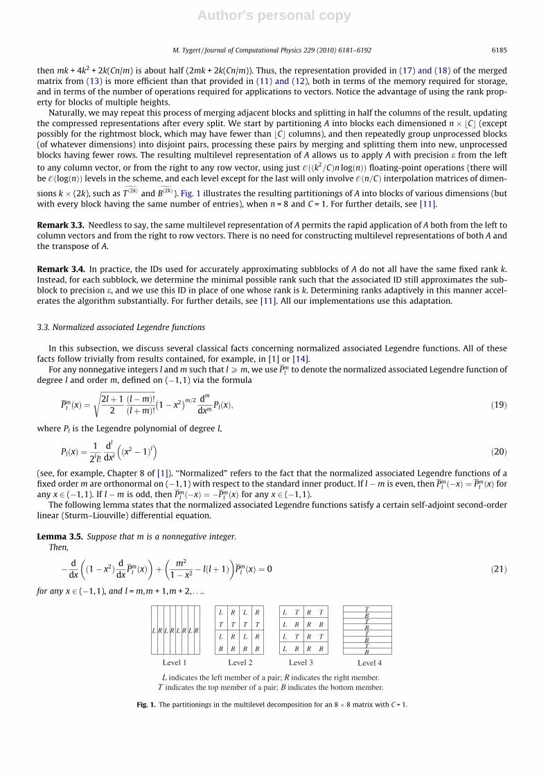
sions k � (2k), such as gT ð2kÞ and gBð2kÞ ). Fig. 1 illustrates the resulting partitionings of A into blocks of various dimensions (butwith every block having the same number of entries), when n = 8 and C = 1. For further details, see [11].

Remark 3.3. Needless to say, the same multilevel representation of A permits the rapid application of A both from the left tocolumn vectors and from the right to row vectors. There is no need for constructing multilevel representations of both A andthe transpose of A.

Remark 3.4. In practice, the IDs used for accurately approximating subblocks of A do not all have the same fixed rank k.Instead, for each subblock, we determine the minimal possible rank such that the associated ID still approximates the sub-block to precision e, and we use this ID in place of one whose rank is k. Determining ranks adaptively in this manner accel-erates the algorithm substantially. For further details, see [11]. All our implementations use this adaptation.

3.3. Normalized associated Legendre functions

In this subsection, we discuss several classical facts concerning normalized associated Legendre functions. All of thesefacts follow trivially from results contained, for example, in [1] or [14].

For any nonnegative integers l and m such that l P m, we use Pml to denote the normalized associated Legendre function of

degree l and order m, defined on (�1,1) via the formula

Pml ðxÞ ¼

ffiffiffiffiffiffiffiffiffiffiffiffiffiffiffiffiffiffiffiffiffiffiffiffiffiffiffiffiffiffiffi2lþ 1

2ðl�mÞ!ðlþmÞ!

s1� x2� �m=2 dm

dxmPlðxÞ; ð19Þ

where Pl is the Legendre polynomial of degree l,

PlðxÞ ¼1

2ll!

dl

dxlðx2 � 1Þl�

ð20Þ

(see, for example, Chapter 8 of [1]). ‘‘Normalized” refers to the fact that the normalized associated Legendre functions of afixed order m are orthonormal on (�1,1) with respect to the standard inner product. If l �m is even, then Pm

l ð�xÞ ¼ Pml ðxÞ for

any x 2 (�1,1). If l �m is odd, then Pml ð�xÞ ¼ �Pm

l ðxÞ for any x 2 (�1,1).The following lemma states that the normalized associated Legendre functions satisfy a certain self-adjoint second-order

linear (Sturm–Liouville) differential equation.

Lemma 3.5. Suppose that m is a nonnegative integer.Then,

� ddxð1� x2Þ d

dxPm

l ðxÞ� �

þ m2

1� x2 � lðlþ 1Þ� �

Pml ðxÞ ¼ 0 ð21Þ

for any x 2 (�1,1), and l = m,m + 1,m + 2, . . ..

Level 1 Level 2 Level 3

R L R L R L RL

L R L R

B

T T T T

B B B

L R L R

L R

L

L

L

R

R

R

T

B

T

T T

B

B B

TBTBTBTB

Level 4

L indicates the left member of a pair; R indicates the right member.T indicates the top member of a pair; B indicates the bottom member.

Fig. 1. The partitionings in the multilevel decomposition for an 8 � 8 matrix with C = 1.



The following lemma states that the normalized associated Legendre function of order m and degree m + 2n has exactly nzeros inside (0,1), and, moreover, that the normalized associated Legendre function of order m and degree m + 2n + 1 also hasexactly n zeros inside (0,1).

Lemma 3.6. Suppose that m and n are nonnegative integers with n > 0.Then, there exist precisely n real numbers x0,x1, . . .,xn�2,xn�1 such that

0 < x0 < x1 < . . . < xn�2 < xn�1 < 1 ð22Þ

and

Pmmþ2nðxjÞ ¼ 0 ð23Þ

for j = 0,1, . . .,n � 2,n � 1.Moreover, there exist precisely n real numbers y0,y1, . . .,yn�2,yn�1 such that

0 < y0 < y1 < . . . < yn�2 < yn�1 < 1 ð24Þ

and

Pmmþ2nþ1ðyjÞ ¼ 0 ð25Þ

for j = 0,1, . . .,n � 2,n � 1.Suppose that m and n are nonnegative integers with n > 0. Then, we define real numbers q0,q1, . . .,qn�2,qn�1,r0,r1, . . .,

rn�2,rn�1, and rn via the formulae

qj ¼2ð2mþ 4nþ 1Þ

1� ðxjÞ2�

ddx Pm

mþ2nðxjÞ� �2 ð26Þ

for j = 0,1, . . .,n � 2,n � 1, where x0,x1, . . .,xn�2,xn�1 are from (23),

rj ¼2ð2mþ 4nþ 3Þ

1� ðyjÞ2

� ddx Pm

mþ2nþ1ðyjÞ� �2 ð27Þ

for j = 0,1, . . .,n � 2,n � 1, where y0,y1, . . .,yn�2,yn�1 are from (25), and

rn ¼2mþ 4nþ 3ddx Pm

mþ2nþ1ð0Þ� �2 : ð28Þ

The following lemma describes what are known as Gauss–Jacobi quadrature formulae corresponding to associated Legen-dre functions.

Lemma 3.7. Suppose that m and n are nonnegative integers with n > 0.Then,Z 1

�1dx 1� x2� �m

pðxÞ ¼Xn�1

j¼0

qj 1� ðxjÞ2� m

pðxjÞ ð29Þ

for any even polynomial p of degree at most 4n � 2, where x0,x1, . . .,xn�2,xn�1 are from (23), and q0,q1, . . .,qn�2,qn�1 are definedin (26).

Furthermore,Z 1

�1dxð1� x2ÞmpðxÞ ¼ rnpð0Þ þ

Xn�1

j¼0

rj 1� ðyjÞ2

� mpðyjÞ ð30Þ

for any even polynomial p of degree at most 4n, where y0,y1, . . .,yn�2,yn�1 are from (25), and r0,r1, . . .,rn�1,rn are defined in (27)and (28).

Remark 3.8. Formulae (35) and (36) of [15] incorrectly omitted the factors (1 � (xj)2)m and (1 � (yj)2)m appearing in the anal-ogous (29) and (30) above.

Suppose that m is a nonnegative integer. Then, we define real numbers cm,cm+1,cm+2, . . . and dm,dm+1,dm+2, . . . via theformulae

cl ¼ffiffiffiffiffiffiffiffiffiffiffiffiffiffiffiffiffiffiffiffiffiffiffiffiffiffiffiffiffiffiffiffiffiffiffiffiffiffiffiffiffiffiffiffiffiffiffiffiffiffiffiffiffiffiffiffiffiffiffiffiffiffiffiffiffiffiffiffiffiffiffiffiffiffiffiffiffiffiffiffiffiffiffiffiffiffiffiffiffiffiffiffiffiffiffiðl�mþ 1Þðl�mþ 2Þðlþmþ 1Þðlþmþ 2Þ

ð2lþ 1Þð2lþ 3Þ2ð2lþ 5Þ

sð31Þ



for l = m,m + 1,m + 2, . . ., and

dl ¼2lðlþ 1Þ � 2m2 � 1ð2l� 1Þð2lþ 3Þ ð32Þ

for l = m,m + 1,m + 2, . . ..The following lemma states that the normalized associated Legendre functions of a fixed order m satisfy a certain three-

term recurrence relation.

Lemma 3.9. Suppose that m is a nonnegative integer.Then,

x2Pml ðxÞ ¼ dlPm

l ðxÞ þ clPmlþ2ðxÞ ð33Þ

for any x 2 (�1,1), and l = m or l = m + 1, and

x2Pml ðxÞ ¼ cl�2Pm

l�2ðxÞ þ dlPml ðxÞ þ clPm

lþ2ðxÞ ð34Þ

for any x 2 (�1,1), and l = m + 2,m + 3,m + 4, . . ., where cm,cm+1,cm+2, . . . are defined in (31), and dm,dm+1,dm+2, . . . are defined in(32).

4. Precomputations for the butterfly scheme

In this section, we discuss the preprocessing required for the butterfly algorithm summarized in Section 3.2. We will beusing the notation detailed in Section 3.2.

Perhaps the most natural organization of the computations required to construct the multilevel representation of an n � nmatrix A is first to process all blocks having n rows (Level 1 in Fig. 1 above), then to process all blocks having about n/2 rows(Level 2 in Fig. 1), then to process all blocks having about n/4 rows (Level 3 in Fig. 1), and so on. Indeed, [11] uses this orga-nization, which amounts to a ‘‘breadth-first traversal” of the control-flow graph for the program applying A to a vector (see,for example, [3] for an introduction to ‘‘breadth-first” and ‘‘depth-first” orderings). This scheme for preprocessing is efficientwhen the entries of A can be efficiently computed on-the-fly, individually. (Of course, we are assuming that A has a suitablerank property, that is, that there are positive real numbers e and C, and a positive integer k, such that any contiguous rect-angular subblock of A containing at most Cn entries can be approximated to precision e by a matrix whose rank is k, using theFrobenius/Hilbert–Schmidt norm to measure the accuracy of the approximation. Often, taking C to be roughly proportionalto k suffices, and ideally k and e are small.) If the entries of A cannot be efficiently computed individually, however, then the‘‘breadth-first traversal” may need to store Oðn2Þ entries at some point during the precomputations, in order to avoid recom-puting entries of the matrix.

If individual columns of A (but not necessarily arbitrary individual entries) can be computed efficiently, then ‘‘depth-first

traversal” of the control-flow graph requires only Oððk2=CÞn logðnÞÞ floating-point words of memory at any point during the

precomputations, for the following reason. We will say that we ‘‘process” a block of A to mean that we merge it with another,and split and recompress the result, producing a pair of new, unprocessed blocks. Rather than starting the preprocessing byconstructing all blocks having n rows, we construct each such block only after processing as many blocks as possible whichprevious processing creates, but which have not yet been processed. Furthermore, we construct each block having n rowsonly after having already constructed (and possibly processed) all blocks to its left. To reiterate, we construct a block havingn rows only after having exhausted all possibilities for both creating and processing blocks to its left.

For each processed block B, we need only store the interpolation matrix gBð2kÞ and the indices of the columns chosen for theID; we need not store the k columns of B(k) selected for the ID, since the algorithm for applying A (or its transpose) to a vectornever explicitly uses any columns of a block that has been merged with another and split, but instead interpolates from (or

anterpolates to) the shorter blocks arising from the processing. Conveniently, the matrix gBð2kÞ that we must store is small —no larger than k � (2k). For each unprocessed block B, we do need to store the k columns in B(k) selected for the ID, in addition

to storing gBð2kÞ and the indices of the columns chosen for the ID, facilitating any subsequent processing. Although B(k) mayhave many rows, it has only as many rows as B and hence is smaller when B has fewer rows. Thus, every time we process apair of tall blocks, producing a new pair of blocks having half as many rows, the storage requirements for all these blockstogether nearly halve. By always processing as many already constructed blocks as possible, we minimize the amount ofmemory required.

5. Spherical harmonic transforms via the butterfly scheme

In this section, we describe how to use the butterfly algorithm to compute fast spherical harmonic transforms, via appro-priate modifications of the algorithm of [15].



We substitute the butterfly algorithm for the divide-and-conquer algorithm of [7] used in Section 3.1 of [15], otherwiseleaving the approach of [15] unchanged. Specifically, given numbers b0,b1, . . .,bn�2,bn�1, we use the butterfly scheme to com-pute the numbers a0,a1, . . .,an�2,an�1 defined via the formula

ai ¼Xn�1

j¼0

bjffiffiffiffiffiqip

Pmmþ2jðxiÞ ð35Þ

for i = 0,1, . . .,n � 2,n � 1, where m is a nonnegative integer, Pmm; P

mmþ2; . . . ; Pm

mþ2n�2; Pmmþ2n are the normalized associated Legendre

functions of order m defined in (19), x0,x1, . . .,xn�2,xn�1 are the positive zeros of Pmmþ2n from (23), and q0,q1, . . .,qn�2,qn�1 are the

corresponding quadrature weights from (29). Similarly, given numbers a0,a1, . . .,an�2,an�1, we use the butterfly scheme tocompute the numbers b0,b1, . . .,bn�2,bn�1 satisfying (35). The factors

ffiffiffiffiffiffiq0p

;ffiffiffiffiffiffiq1p

; . . . ;ffiffiffiffiffiffiffiffiffiffiqn�2p

;ffiffiffiffiffiffiffiffiffiffiqn�1p

ensure that the linear trans-formation mapping b0,b1, . . .,bn�2,bn�1 to a0,a1, . . .,an�2,an�1 via (35) is unitary (due to (19), (29), and the orthonormality of thenormalized associated Legendre functions on (�1,1)), so that the inverse of the linear transformation is its transpose.

Moreover, given numbers m0,m1, . . .,mn�2,mn�1, we use the butterfly scheme to compute the numbers l0,l1, . . .,ln�2,ln�1

defined via the formula

li ¼Xn�1

j¼0

mjffiffiffiffiffirip

Pmmþ2jþ1ðyiÞ ð36Þ

for i = 0,1, . . .,n � 2,n � 1, where m is a nonnegative integer, Pmmþ1; P

mmþ3; . . . ; Pm

mþ2n�1; Pmmþ2nþ1 are the normalized associated

Legendre functions of order m defined in (19), y0,y1, . . .,yn�2,yn�1 are the positive zeros of Pmmþ2nþ1 from (25), and

r0,r1, . . .,rn�2,rn�1 are the corresponding quadrature weights from (30). Similarly, given numbers l0,l1, . . .,ln�2,ln�1, weuse the butterfly scheme to compute the numbers m0,m1, . . .,mn�2,mn�1 satisfying (36). As above, the factorsffiffiffiffiffiffir0p

;ffiffiffiffiffiffir1p

; . . . ;ffiffiffiffiffiffiffiffiffiffirn�2p

;ffiffiffiffiffiffiffiffiffiffirn�1p

ensure that the linear transformation mapping m0,m1, . . .,mn�2,mn�1 to l0,l1, . . .,ln�2,ln�1 via(36) is unitary, so that its inverse is its transpose.

Computing spherical harmonic transforms requires several additional computations, detailed in [15]. (See also Remark5.1 below.) The butterfly algorithm replaces only the procedure described in Section 3.1 of [15].

In order to use (35) and (36) numerically, we need to precompute the positive zeros x0,x1, . . .,xn�2,xn�1 of Pmmþ2n from (23),

the corresponding quadrature weights q0,q1, . . .,qn�2,qn�1 from (29), the positive zeros y0,y1, . . .,yn�2,yn�1 of Pmmþ2nþ1 from

(25), and the corresponding quadrature weights r0,r1, . . .,rn�2,rn�1 from (30). Section 3.3 of [15] describes suitable proce-dures (based on integrating the ordinary differential equation in (21) in ‘‘Prüfer coordinates”). We found it expedient to per-form this preprocessing in extended-precision arithmetic, in order to compensate for the loss of a couple of digits of accuracyrelative to the machine precision.

To perform the precomputations described in Section 4 above associated with (35) and (36), we need to be able to eval-uate efficiently all n functions Pm

m; Pmmþ2; . . . ; Pm

mþ2n�4; Pmmþ2n�2 at any of the precomputed positive zeros x0,x1, . . .,xn�2,xn�1 of

Pmmþ2n from (23), and, similarly, we need to be able to evaluate efficiently all n functions Pm

mþ1; Pmmþ3; . . . ; Pm

mþ2n�3; Pmmþ2n�1 at

any of the precomputed positive zeros y0,y1, . . .,yn�2,yn�1 of Pmmþ2nþ1 from (25). For this, we may use the recurrence relations

(33) and (34), starting with the values of PmmðxiÞ; Pm

mþ1ðyiÞ; Pmmþ2ðxiÞ, and Pm

mþ3ðyiÞ obtained via (19). (We can counter underflowby tracking exponents explicitly, in the standard fashion.) Such use of the recurrence is a classic procedure; see, for example,Chapter 8 of [1]. The recurrence appears to be numerically stable when used for evaluating normalized associated Legendrefunctions of order m and of degrees at most m + 2n � 1, at these special points x0,x1, . . .,xn�2,xn�1 and y0,y1, . . .,yn�2,yn�1, evenwhen n is very large. We did not need to use extended-precision arithmetic for this preprocessing.

Remark 5.1. The formula (88) in [15] that is analogous to (35) of the present paper omits the factorsffiffiffiffiffiffiq0p

;ffiffiffiffiffiffiq1p

; . . . ;ffiffiffiffiffiffiffiffiffiffiqn�2p

;ffiffiffiffiffiffiffiffiffiffiqn�1p

included in (35). Obviously, the vectors

ða0;a1; . . . ;an�2;an�1Þ> ð37Þ

and

a0ffiffiffiffiffiffiq0p ;

a1ffiffiffiffiffiffiq1p ; . . . ;

an�2ffiffiffiffiffiffiffiffiffiffiqn�2p ;

an�1ffiffiffiffiffiffiffiffiffiffiqn�1p

� �>ð38Þ

differ by a diagonal transformation, and so we can obtain either one from the other efficiently. In fact, the well-conditionedmatrix A from Section 3.1 of [15] represents the same diagonal transformation, mapping (37) to (38). Similar remarks applyto (36), of course.

6. Numerical results

In this section, we describe the results of several numerical tests of the algorithm of the present paper. (Computing spher-ical harmonic transforms requires several additional computations, detailed in [15] — see Section 5 for further information.The butterfly algorithm replaces only the procedure described in Section 3.1 of [15].)



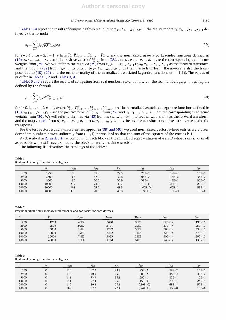
Tables 1–4 report the results of computing from real numbers b0,b1, . . .,bn�2,bn�1 the real numbers a0,a1, . . .,an�2,an�1 de-fined by the formula

ai ¼Xn�1

j¼0

bjffiffiffiffiffiqip

Pmmþ2jðxiÞ ð39Þ

for i = 0,1, . . .,n � 2,n � 1, where Pmm; P

mmþ2; . . . ; Pm

mþ2n�2; Pmmþ2n are the normalized associated Legendre functions defined in

(19), x0,x1, . . .,xn�2,xn�1 are the positive zeros of Pmmþ2n from (23), and q0,q1, . . .,qn�2,qn�1 are the corresponding quadrature

weights from (29). We will refer to the map via (39) from b0,b1, . . .,bn�2,bn�1 to a0,a1, . . .,an�2,an�1 as the forward transform,and the map via (39) from a0,a1, . . .,an�2,an�1 to b0,b1, . . .,bn�2,bn�1 as the inverse transform (the inverse is also the trans-pose, due to (19), (29), and the orthonormality of the normalized associated Legendre functions on (�1,1)). The values ofm differ in Tables 1, 2 and Tables 3, 4.

Tables 5 and 6 report the results of computing from real numbers m0,m1, . . .,mn�2,mn�1 the real numbers l0,l1, . . .,ln�2,ln�1

defined by the formula

li ¼Xn�1

j¼0

mjffiffiffiffiffirip

Pmmþ2jþ1ðyiÞ ð40Þ

for i = 0,1, . . .,n � 2,n � 1, where Pmmþ1; P

mmþ3; . . . ; Pm

mþ2n�1; Pmmþ2nþ1 are the normalized associated Legendre functions defined in

(19), y0,y1, . . .,yn�2,yn�1 are the positive zeros of Pmmþ2nþ1 from (25), and r0,r1, . . .,rn�2,rn�1 are the corresponding quadrature

weights from (30). We will refer to the map via (40) from m0,m1, . . .,mn�2,mn�1 to l0,l1, . . .,ln�2,ln�1 as the forward transform,and the map via (40) from l0,l1, . . .,ln�2,ln�1 to m0,m1, . . .,mn�2,mn�1 as the inverse transform (as above, the inverse is also thetranspose).

For the test vectors b and m whose entries appear in (39) and (40), we used normalized vectors whose entries were pseu-dorandom numbers drawn uniformly from (�1,1), normalized so that the sum of the squares of the entries is 1.

As described in Remark 3.4, we compute for each block in the multilevel representation of A an ID whose rank is as smallas possible while still approximating the block to nearly machine precision.

The following list describes the headings of the tables:

Table 1Ranks and running-times for even degrees.

n m kmax kavg kr tdir tfwd tinv

1250 1250 170 65.3 29.5 .25E�2 .18E�2 .15E�22500 2500 168 67.0 32.6 .98E�2 .46E�2 .38E�25000 5000 195 70.5 35.9 .39E�1 .12E�1 .96E�2

10000 10000 247 73.5 38.7 .15E�0 .28E�1 .23E�120000 20000 308 75.9 41.5 (.60E�0) .67E�1 .55E�140000 40000 379 78.0 43.8 (.24E+1) .16E�0 .13E�0

Table 2Precomputation times, memory requirements, and accuracies for even degrees.

n m tquad tcomp mmax efwd einv

1250 1250 .46E2 .96E0 .86E6 .62E�14 .19E�132500 2500 .92E2 .41E1 .20E7 .37E�14 .25E�135000 5000 .18E3 .17E2 .50E7 .59E�14 .43E�13


Table 3Ranks and running-times for even degrees.


1250 0 110 67.0 23.3 .25E�2 .18E�2 .15E�22500 0 110 70.0 25.0 .98E�2 .48E�2 .40E�25000 0 111 73.9 26.1 .39E�1 .12E�1 .10E�1

10000 0 111 77.3 26.8 .15E�0 .29E�1 .24E�120000 0 112 80.2 27.1 (.60E�0) .68E�1 .57E�140000 0 169 82.7 27.4 (.24E+1) .16E�0 .13E�0



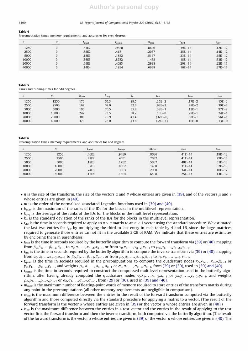
� n is the size of the transform, the size of the vectors a and b whose entries are given in (39), and of the vectors l and mwhose entries are given in (40).� m is the order of the normalized associated Legendre functions used in (39) and (40).� kmax is the maximum of the ranks of the IDs for the blocks in the multilevel representation.� kavg is the average of the ranks of the IDs for the blocks in the multilevel representation.� kr is the standard deviation of the ranks of the IDs for the blocks in the multilevel representation.� tdir is the time in seconds required to apply an n � n matrix to an n � 1 vector using the standard procedure. We estimated

the last two entries for tdir by multiplying the third-to-last entry in each table by 4 and 16, since the large matricesrequired to generate those entries cannot fit in the available 2 GB of RAM. We indicate that these entries are estimatesby enclosing them in parentheses.� tfwd is the time in seconds required by the butterfly algorithm to compute the forward transform via (39) or (40), mapping

from b0,b1, . . .,bn�2,bn�1 to a0,a1, . . .,an�2,an�1, or from m0,m1, . . .,mn�2,mn�1 to l0,l1, . . .,ln�2,ln�1.� tinv is the time in seconds required by the butterfly algorithm to compute the inverse transform via (39) or (40), mapping

from a0,a1, . . .,an�2,an�1 to b0,b1, . . .,bn�2,bn�1, or from l0,l1, . . .,ln�2,ln�1 to m0,m1, . . .,mn�2,mn�1.� tquad is the time in seconds required in the precomputations to compute the quadrature nodes x0,x1, . . .,xn�2,xn�1 or

y0,y1, . . .,yn�2,yn�1, and weights q0,q1, . . .,qn�2,qn�1 or r0,r1, . . .,rn�2,rn�1, from (29) or (30), used in (39) and (40).� tcomp is the time in seconds required to construct the compressed multilevel representation used in the butterfly algo-

rithm, after having already computed the quadrature nodes x0,x1, . . .,xn�2,xn�1 or y0,y1, . . .,yn�2,yn�1, and weightsq0,q1, . . .,qn�2,qn�1 or r0,r1, . . .,rn�2,rn�1, from (29) or (30), used in (39) and (40).� mmax is the maximum number of floating-point words of memory required to store entries of the transform matrix during

any point in the precomputations (all other memory requirements are negligible in comparison).� efwd is the maximum difference between the entries in the result of the forward transform computed via the butterfly

algorithm and those computed directly via the standard procedure for applying a matrix to a vector. (The result of theforward transform is the vector a whose entries are given in (39) or the vector l whose entries are given in (40).)� einv is the maximum difference between the entries in a test vector and the entries in the result of applying to the test

vector first the forward transform and then the inverse transform, both computed via the butterfly algorithm. (The resultof the forward transform is the vector a whose entries are given in (39) or the vector l whose entries are given in (40). The

Table 4Precomputation times, memory requirements, and accuracies for even degrees.




Table 5Ranks and running-times for odd degrees.


1250 1250 170 65.3 29.5 .25E�2 .17E�2 .15E�22500 2500 169 67.0 32.6 .98E�2 .48E�2 .39E�25000 5000 196 70.5 35.9 .39E�1 .12E�1 .97E�2

10000 10000 247 73.5 38.7 .15E�0 .28E�1 .24E�120000 20000 308 75.9 41.4 (.60E�0) .68E�1 .56E�140000 40000 379 78.0 43.8 (.24E+1) .16E�0 .13E�0

Table 6Precomputation times, memory requirements, and accuracies for odd degrees.






result of the inverse transform is the vector b whose entries are given in (39) or the vector m whose entries are given in(40).) Thus, einv measures the accuracy of the butterfly algorithm without reference to the standard procedure for apply-ing a matrix to a vector (unlike efwd).

For the first level of the multilevel representation of the n � n matrix, we partitioned the matrix into blocks each dimen-sioned n � 60 (except for the rightmost block, since n is not divisible by 60). Every block on every level has about the samenumber of entries (specifically, 60n entries). We wrote all code in Fortran 77, compiling it using the Lahey–Fujitsu Linux Ex-press v6.2 compiler, with optimization flag --o2 enabled. We ran all examples on one core of a 2.7 GHz Intel Core 2 Duomicroprocessor with 3 MB of L2 cache and 2 GB of RAM. As described in Section 5, we used extended-precision arithmeticduring the portion of the preprocessing requiring integration of an ordinary differential equation, to compute quadraturenodes and weights (this is not necessary to attain high accuracy, but does yield a couple of extra digits of precision). Other-wise, our code is compliant with the IEEE double-precision standard (so that the mantissas of variables have approximatelyone bit of precision less than 16 digits, yielding a relative precision of about .2E–15).

Remark 6.1. Tables 1, 3, and 5 indicate that the linear transformations in (39) and (40) satisfy the rank property discussed inSection 3.2, with arbitrarily high precision, at least in some averaged sense. Furthermore, it appears that the parameter kdiscussed in Section 3.2 can be set to be independent of the order m and size n of the transforms in (39) and (40), with theparameter C discussed in Section 3.2 roughly proportional to k. The acceleration provided by the butterfly algorithm thus issufficient for computing fast spherical harmonic transforms, and is competitive with the approach taken in [15] (thoughmuch work remains in optimizing both approaches in order to gauge their relative performance). Unlike the approach takenin [15], the approach of the present paper does not require the use of extended-precision arithmetic during theprecomputations in order to attain accuracy close to the machine precision, even while accelerating spherical harmonictransforms about as well. Moreover, the butterfly can be easier to implement.

Remark 6.2. The values in Tables 2, 4, and 6 vary with the size n of the transforms in (39) and (40) as expected. The valuesfor tquad are consistent with the expected values of a constant times n. The values for tcomp are consistent with the expectedvalues of a constant times n2 (with the constant being proportional to kavg). The values for mmax are consistent with theexpected values of a constant times n log(n) (again with the constant being proportional to kavg); these modest memoryrequirements make the preprocessing feasible for large values of n such as those in the tables.

Remark 6.3. In the current technological environment, neither the scheme of [15] nor the approach of the present paper isuniformly superior to the other. For example, the theory from [15] is rigorous and essentially complete, while the theory ofthe present article ideally should undergo further development, to prove that the rank properties discussed in Remark 6.1 areas strong as numerical experiments indicate, yielding the desired acceleration. In contrast, to attain accuracy close to themachine precision, the approach of [15] requires the use of extended-precision arithmetic during its precomputations,whereas the scheme of the present paper does not. Implementing the procedure of the present article can be easier. Finally,an anonymous referee kindly compared the running-times of the implementations reported in [15] and the present paper,noticing that the newer computer system used in the present article is about 2.7 times faster than the old system; the algo-rithms of [15] and of the present article are roughly equally efficient — certainly neither appears to be more than twice fasterthan the other. However, both implementations are rather crude, and could undoubtedly benefit from further optimizationby experts on computer architectures; also, we made no serious attempt to optimize the precomputations. Furthermore,with the advent of multicore and distributed processors, coming changes in computer architectures might affect the twoapproaches differently, as they may parallelize and utilize cache in different ways. In the end, the use of one approach ratherthan the other may be a matter of convenience, as the two methods are yielding similar performance.

7. Conclusions

This article provides an alternative means for performing the key computational step required in [15] for computing fastspherical harmonic transforms. Unlike the implementation described in [15] of divide-and-conquer spectral methods, thebutterfly scheme of the present paper does not require the use of extended precision during the compression precomputa-tions in order to attain accuracy very close to the machine precision. With the butterfly, the required amount of preprocess-ing is quite reasonable, certainly not prohibitive.

Unfortunately, there seems to be little theoretical understanding of why the butterfly procedure works so well for asso-ciated Legendre functions (are the associated transforms nearly weighted averages of Fourier integral operators?). Completeproofs such as those in [11,15] are not yet available for the scheme of the present article. By construction, the butterfly en-ables fast, accurate applications of matrices to vectors when the precomputations succeed. However, we have yet to provethat the precomputations will compress the appropriate n � n matrix enough to enable applications of the matrix to vectorsusing only Oðn logðnÞÞ floating-point operations (flops). Nevertheless, the scheme has succeeded in all our numerical tests.We hope to produce rigorous mathematical proofs that the precomputations always compress the matrices as much as theydid in our numerical experiments.



The precomputations for the algorithm of the present article require Oðn2Þ flops. The precomputations for the algorithm of[15] also require Oðn2Þ flops as implemented for the numerical examples of that paper; however, the procedure of [7] leadsnaturally to precomputations for the approach of [15] requiring only Oðn logðnÞÞ flops (though these ‘‘more efficient” precom-putations do not become more efficient in practice until n is absurdly large, too large even to estimate reliably). We do notexpect to be able to accelerate the precomputations for the algorithm of the present article without first producing the rig-orous mathematical proofs mentioned in the previous paragraph. Even so, the current amount of preprocessing is not unrea-sonable, as the numerical examples of Section 6 illustrate.

Acknowledgements

We would like to thank V. Rokhlin for his advice, for his encouragement, and for the use of his software libraries, all ofwhich have greatly enhanced this paper and the associated computer codes. We are also grateful to R.R. Coifman and Y.Shkolnisky. We would like to thank the anonymous referees for their useful suggestions.

References

[1] M. Abramowitz, I.A. Stegun (Eds.), Handbook of Mathematical Functions, Dover Publications, New York, 1972.[2] J.C. Adams, P.N. Swarztrauber, SPHEREPACK 3.0: A model development facility, Mon. Wea. Rev. 127 (1999) 1872–1878.[3] A. Aho, J. Hopcroft, J. Ullman, Data Structures and Algorithms, Addison-Wesley, 1987.[4] E. Candès, L. Demanet, L. Ying, A fast butterfly algorithm for the computation of Fourier integral operators, Multiscale Model. Simul. 7 (4) (2009) 1727–

1750.[5] H. Cheng, Z. Gimbutas, P.-G. Martinsson, V. Rokhlin, On the compression of low rank matrices, SIAM J. Sci. Comput. 26 (4) (2005) 1389–1404.[6] S.A. Goreinov, E.E. Tyrtyshnikov, The maximal-volume concept in approximation by low-rank matrices, in: V. Olshevsky (Ed.), Structured Matrices in

Mathematics, Computer Science, and Engineering I: Proceedings of an AMS-IMS-SIAM Joint Summer Research Conference, University of Colorado,Boulder, June 27–July 1, 1999, vol. 280 of Contemporary Mathematics, AMS Publications, Providence, RI, 2001, pp. 47–51.

[7] M. Gu, S.C. Eisenstat, A divide-and-conquer algorithm for the symmetric tridiagonal eigenproblem, SIAM J. Matrix Anal. Appl. 16 (1995) 172–191.[8] M. Gu, S.C. Eisenstat, Efficient algorithms for computing a strong rank-revealing QR factorization, SIAM J. Sci. Comput. 17 (4) (1996) 848–869.[9] P.-G. Martinsson, V. Rokhlin, M. Tygert, On interpolation and integration in finite-dimensional spaces of bounded functions, Commun. Appl. Math.

Comput. Sci. 1 (2006) 133–142.[10] E. Michielssen, A. Boag, A multilevel matrix decomposition algorithm for analyzing scattering from large structures, IEEE Trans. Antennas Propag. 44

(8) (1996) 1086–1093.[11] M. O’Neil, F. Woolfe, V. Rokhlin, An algorithm for the rapid evaluation of special function transforms, Appl. Comput. Harmon. Anal. 28 (2) (2010) 203–

226.[12] M.G. Reuter, M.A. Ratner, T. Seideman, A fast method for solving both the time-dependent Schrödinger equation in angular coordinates and its

associated ‘‘m-mixing” problem, J. Chem. Phys. 131 (2009) 094108-1–094108-6.[13] P.N. Swarztrauber, W.F. Spotz, Generalized discrete spherical harmonic transforms, J. Comput. Phys. 159 (2) (2000) 213–230.[14] G. Szegö, Orthogonal Polynomials, eleventh ed., vol. 23, Colloquium Publications, American Mathematical Society, Providence, RI, 2003.[15] M. Tygert, Fast algorithms for spherical harmonic expansions, II, J. Comput. Phys. 227 (8) (2008) 4260–4279.[16] E.E. Tyrtyshnikov, Incomplete cross approximation in the mosaic-skeleton method, Computing 64 (4) (2000) 367–380.[17] L. Ying, Sparse Fourier transform via butterfly algorithm, SIAM J. Sci. Comput. 31 (3) (2009) 1678–1694.


Documents

Author's personal copy - Mark Tygert's homepagetygert.com/butterfly.pdfAuthor's personal copy Short Note Fast algorithms for spherical harmonic expansions, III Mark Tygert Courant