Author's personal copy - Faculdade de Engenharia da

This article appeared in a journal published by Elsevier. The attachedcopy is furnished to the author for internal non-commercial researchand education use, including for instruction at the authors institution

and sharing with colleagues.

Other uses, including reproduction and distribution, or selling orlicensing copies, or posting to personal, institutional or third party

websites are prohibited.

In most cases authors are permitted to post their version of thearticle (e.g. in Word or Tex form) to their personal website orinstitutional repository. Authors requiring further information

regarding Elsevier’s archiving and manuscript policies areencouraged to visit:

http://www.elsevier.com/copyright

http://www.elsevier.com/copyright

Author's personal copy

J. Non-Newtonian Fluid Mech. 165 (2010) 247–262

Contents lists available at ScienceDirect

Journal of Non-Newtonian Fluid Mechanics

journa l homepage: www.e lsev ier .com/ locate / jnnfm

Numerical solution of the PTT constitutive equation for unsteadythree-dimensional free surface flows

M.F. Toméa,∗, G.S. Pauloa,1, F.T. Pinhob, M.A. Alvesc

a Departamento de Matemática Aplicada e Estatística, Instituto de Ciências Matemáticas e de Computacão, Universidade de São Paulo, Av. Trabalhador Sãocarlense,400 - Caixa Postal 668, CEP 13560-970, São Carlos, SP, Brazilb CEFT - Departamento de Engenharia Mecânica - Faculdade de Engenharia da Universidade do Porto Rua Dr. Roberto Frias s/n, 4200-465 Porto, Portugalc CEFT - Departamento de Engenharia Química - Faculdade de Engenharia da Universidade do Porto, Rua Dr. Roberto Frias s/n, 4200-465 Porto, Portugal

a r t i c l e i n f o

Article history:Received 18 June 2009Received in revised form 5 November 2009Accepted 23 December 2009

Three-dimensional viscoelastic flowFree surfacePTT modelFinite differenceMarker-and-cellJet bucklingExtrudate swell

a b s t r a c t

This work deals with the development of a numerical technique for simulating three-dimensionalviscoelastic free surface flows using the PTT (Phan-Thien–Tanner) nonlinear constitutive equation. Inparticular, we are interested in flows possessing moving free surfaces. The equations describing thenumerical technique are solved by the finite difference method on a staggered grid. The fluid is modelledby a Marker-and-Cell type method and an accurate representation of the fluid surface is employed. Thefull free surface stress conditions are considered. The PTT equation is solved by a high order method,which requires the calculation of the extra-stress tensor on the mesh contours. To validate the numericaltechnique developed in this work flow predictions for fully developed pipe flow are compared with ananalytic solution from the literature. Then, results of complex free surface flows using the PTT equationsuch as the transient extrudate swell problem and a jet flowing onto a rigid plate are presented. Aninvestigation of the effects of the parameters ε and � on the extrudate swell and jet buckling problems isreported.

© 2010 Elsevier B.V. All rights reserved.

1. Introduction

Industrial flows of viscoelastic materials, such as polymer melts,often involve non-isothermal three-dimensional flow with mul-tiple moving free surfaces. From a numerical point of view thecorresponding free surface conditions are not yet satisfactorilydealt with. Some of the difficulties relate to the treatment of theadvective terms in the rheological constitutive equation and how toaccurately impose the free surface stress conditions. Nonetheless,many authors have developed a variety of numerical techniquesfor simulating viscoelastic free surface flows. For instance, Keun-ings and his co-workers were among the earliest contributorsto viscoelastic two-dimensional free surface flows (e.g. [7,8,15]).Other classical works in the field were, for instance, the earlyattempts at simulating extrudate swell of an upper convectedMaxwell (UCM) fluid by Tanner [28] and Ryan and Dutta [27].Crochet and Keunings [10] presented a methodology for solvingcircular and planar extrudate swell using the Oldroyd-B model and

∗ Corresponding author. Tel.: +55 16 3307 1942; fax: +55 16 3371 2238.E-mail addresses: [email protected] (M.F. Tomé), [email protected]

(G.S. Paulo), [email protected] (F.T. Pinho), [email protected] (M.A. Alves).1 Currently at Departamento de Matemática, Estatística e Computacão, Universi-

dade Estadual Paulista, Brazil. Tel.: +55 16 3307 1942; fax: +55 16 3371 2238.

compared favourably their numerical results with available exper-imental data. Literature on three-dimensional flows with movingfree surfaces are scarce (e.g. [6,9,13,30,31]). Among the constitutivemodels used, the nonlinear Phan-Thien–Tanner (PTT) constitu-tive equation provides a better fitting to the rheology of polymermelts and concentrated solutions than other simpler models suchas the UCM or Oldroyd-B. This fact, amongst others, motivatedvarious researchers to solve contraction flows in two and threedimensions using the PTT model (see [2–4,35,36]), but its appli-cation to three-dimensional free surface flows has not yet beendemonstrated.

In this work we present a numerical method capable of simu-lating three-dimensional free surface flows governed by the PTTconstitutive equation. It is an extension to three dimensions of thetwo-dimensional technique presented by Paulo et al. [19,21]. Thenumerical technique is based on the discretization by the finitedifference scheme on a staggered grid while the fluid is tracedby a Marker-and-Cell approach [13]. The numerical results werevalidated against the analytic solution of Alves et al. [1] for fullydeveloped pipe flow of PTT fluids. Then, results obtained from thesimulation of three-dimensional problems involving moving freesurfaces, such as jet buckling and the time-dependent extrudateswell, are given. Moreover, an investigation of the effects of thePTT parameters ε and � on the extrudate swell and jet buckling wasperformed.

0377-0257/$ – see front matter © 2010 Elsevier B.V. All rights reserved.doi:10.1016/j.jnnfm.2009.12.007


248 M.F. Tomé et al. / J. Non-Newtonian Fluid Mech. 165 (2010) 247–262

2. Governing equations

The equations governing incompressible isothermal flows arethe mass conservation equation

∂ui∂xi

= 0, (1)

and the equation of motion

�DuiDt

= − ∂p∂xi

+ ∂�ik∂xk

+ �gi (2)

where t is the time,ui is the velocity vector, p is the pressure,� is thefluid density, gi is the gravitational field and �ij is the extra-stresstensor. The symbol D/Dt = (∂(•)/∂t) + (∂(uk •)/∂xk) represents thematerial derivative. In this work we shall be concerned with flows ofviscoelastic fluids governed by the nonlinear constitutive equationPTT (Phan-Thien–Tanner) (see [22])

f (�kk)�ij + ��ij = 2�Dij (3)

where

Dij = 12

(∂uj∂xi

+ ∂ui∂xj

)is the rate of deformation tensor, � is the fluid relaxation time and� is the polymer viscosity coefficient. f (�kk) is the linearized stresscoefficient function, proposed in the original paper of Phan-Thienand Tanner [22] and is given by

f (�kk) = 1 + �ε

��kk. (4)

The symbol (�· ) represents the Gordon–Schowalter convected

derivative defined as Eq. (5)

��ij = D�ij

Dt− �jk

(∂ui∂xk

− �Dik)

− �ik(∂uj∂xk

− �Djk). (5)

The positive parameters ε and � can be used to control viscoelasticproperties, such as the amount of strain-hardening in extensionalflow and the second normal stress difference coefficient in shearflow, respectively.

2.1. Problem formulation

To solve Eqs. (1)–(3) the EVSS transformation (Elastic-ViscousStress-Splitting) [23] is adopted. This formulation splits the poly-mer extra-stress tensor �ij into the sum of a Newtonian contribution2�Dij and an elastic contribution represented by tensor Sij , accord-ing to

�ij = 2�Dij + Sij. (6)

Back-substituting Eq. (6) into Eqs. (2), (3) and (5) we obtain thetransformed equations which we write in non-dimensional form:

∂ui∂t

+ ∂(uk ui)∂xk

= − ∂p∂xi

+ 1Re

∂2ui∂xk∂xk

+ ∂Sik∂xk

+ 1Fr2gi, (7)

f (Skk)Sij +We�Sij = 2

1Re

[1 − f (Skk)]Dij − 2We

Re

�Dij (8)

where f (Skk) = 1 + εReWe(Skk); Re = �UL/�, We = �U/L and Fr =U/√L g denote the Reynolds, Weissenberg and Froude numbers,

respectively. In these non-dimensional numbers, g is the gravita-tional constant and U, L, � and � denote typical velocity, length,density and viscosity scales, respectively. Equations above werenormalized according to

xk = Lxk, ui = Uui, Sij = �U2Sij, gi = ggi,

t = (L/U)t, p = �U2p,

where the overbars indicate the non-dimensional quanti-ties. For conciseness the overbars were dropped in Eqs. (7)and (8), whereas the mass conservation Eq. (1) remainsunchanged.

3. Boundary conditions

To solve Eqs. (1), (7) and (8) we need to specify appropri-ate boundary conditions for ui. For the momentum equation, weemploy the no-slip condition (ui = 0) on stationary rigid bound-aries. At fluid entrances (inflows) the normal velocityun is specifiedwhile the two tangential components ut1 and ut2 are set to zero. Onoutflows (fluid exits) we impose homogeneous Neumann condi-tions, namely ∂un/∂n = 0, ∂ut1/∂n = 0 and ∂ut2/∂n = 0.

3.1. Free surface stress conditions

We shall consider unsteady free surface flows of a viscoelasticfluid moving into a passive atmosphere (which we may take to be atzero relative pressure). In the absence of surface tension effects thenormal and tangential components of the stress must be continu-ous across any free surface, so that on such a surface (see Batchelor[5])

niijnj = 0, t1iijnj = 0, t2iijnj = 0, (9)

where ni as before, denotes unit normal vector to the surface, t1iand t2i denote the two unit tangential vectors to the surface and ijis the normalized total stress tensor given by

ij = −pıij +2ReDij + Sij.

4. Computation of the stress on mesh boundaries

When solving the constitutive equation it is necessary to employan appropriate effective method to approximate the derivativesof the advective terms in order to obtain accurate results andavoid unphysical solutions. In this work we employ the highorder stabilized upwind scheme CUBISTA developed by Alves etal. [2] for viscoelastic models. This scheme requires the valuesof a generic variable, say , that can be positioned upstream(U), downstream (D) or remote-upstream (R) with respect toa reference point (see Fig. 1) at which the variable is being approx-imated (P). Therefore, when calculating the advective terms ofthe stress equations near boundaries, the values of the compo-nents of the non-Newtonian stress tensor on mesh boundaries

Fig. 1. Reference points used for the CUBISTA upwind scheme.


M.F. Tomé et al. / J. Non-Newtonian Fluid Mech. 165 (2010) 247–262 249

are required. We point out that many authors do not com-pute the non-Newtonian stress tensor on rigid boundaries andtherefore when calculating the non-Newtonian stress tensor onpoints that lie near the boundaries (e.g. rigid walls, outflows)they employ a lower order method, often the first order upwindscheme.

To compute the non-Newtonian stress tensor on rigid walls weemploy a methodology similar to that used by Tomé et al. [33] forthe flow of an Oldroyd-B fluid in two dimensions. First we makethe change of variables Sij = e−(1/We)t Sij in Eq. (8) and obtain theequation:

e−1We t[f (Sij) − 1]Sij +We

�Sij = 2

1Re

[1 − f (Sij)]Dij − 2e1We tWe

Re

�Dij.

(10)

Eq. (10) provides a (6 × 6)-nonlinear system for the componentsof tensor Sij . We use the no-slip condition and solve this systemanalytically. The details of the analytic solution of this nonlinearsystem are given in Appendix A.

4.1. Computation of the non-Newtonian stress tensor on inflowand outflow boundaries

These can be specified as follows:

Inflow boundary: If the velocity at the fluid entrance un is con-stant then we follow the strategy of Crochet and Marchal [16] andMompean and Deville [17], namely:

Sij = 0.

For fully developed pipe flows there is a complete analytic solutionof the stress equations which is given in Section 7.Outflow boundary: At the fluid exit, we impose homogeneous Neu-mann conditions for the components of non-Newtonian stresstensor (see [17,33]) namely

∂Sij∂n

= 0.

5. GENSMAC-PTT3D

The method of solution is based on the ideas of Tomé et al. [31]for an Oldroyd-B fluid. It is an extension of the numerical methoddeveloped by Paulo et al. [21] for simulating two-dimensional vis-coelastic free surface flows governed by the PTT model. We solvethe momentum equations followed by the solution of the consti-tutive equation. Thus, to solve Eqs. (1), (7) and (8) we proceed asfollows.

We assume that at time t0 the velocity field ui(xl, t0) and thenon-Newtonian stress tensor Sij(xl, t0) are known and the values ofui and Sij on the boundary are given. The new fields ui(xl, t), p(xl, t)and Sij(xl, t), at the new time level t = t0 + ıt, are calculated asfollows:

Step 1: Let p(xl, t) be a pressure field that satisfies the correct pres-sure condition on the free surface (9).

Step 2: Calculate the intermediate velocity field ui(xl, t) from themomentum equation

∂ui∂t

= −∂(uk ui)∂xk

− ∂p

∂xi+ 1Re

∂2ui∂xk∂xk

+ ∂Sik∂xk

+ 1Fr2gi, (11)

with ui(xl, t) = ui(xl, t0) and it must obey the same bound-ary conditions of velocity ui(xl, t).

Step 3: Solve the Poisson equation for the potential function (xl, t)

∂2 (xl, t)∂xk∂xk

= ∂uk(xl, t)∂xk

(12)

subject to the boundary conditions (see Tomé and McKee[34]): ∂ /∂n = 0 on rigid boundary and inflows and = 0on free surfaces and outflows.

Step 4: Compute the final velocity

ui(xl, t) = ui(xl, t) − ∂ (xl, t)∂xk

. (13)

Step 5: Compute the pressure field from (see Tomé et al. [32])

p(xl, t) = p(xl, t) + (xl, t)ıt

. (14)

Step 6: Calculation of the non-Newtonian tensor Sij(xl, t)6.1 Update the non-Newtonian tensor on rigid boundaries

according to the equations derived in Section 4.6.2 Update the non-Newtonian tensor on inflows

and outflows according to the equations given inSection 4.1.

6.3 Compute the non-Newtonian tensor Sij(xl, t) elsewherefrom Eq. (8).

Step 7: Update the markers positions: the last step in the calcula-tion is to move the markers to their new positions. This isperformed by solving

dxidt

= ui, (15)

for each particle. The fluid surface is defined by a piecewiselinear surface composed of triangles and quadrilateralshaving marker particles on their vertices. For details seeCastelo et al. [9].

6. Finite difference approximation

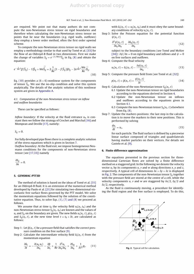
The equations presented in the previous section for three-dimensional Cartesian flows are solved by a finite differencemethod on a staggered grid. In the following we denote the velocityvector ui by its components u, v and w along directions x, y and z,respectively. A typical cell of dimensions ıx × ıy× ız is displayedin Fig. 2. The components of the non-Newtonian tensor Sij togetherwith the pressure field are stored at the centre of a cell, while thevelocity components u, v and w are staggered by ıx/2, ıy/2 andız/2, respectively.

As the fluid is continuously moving, a procedure for identify-ing the fluid region and the free surface is employed. To do this,

Fig. 2. Typical cell for calculation.



the cells within the mesh are flagged as: Empty (E) – cells that donot contain fluid; Full (F) – Cells full of fluid that do not share aface with an Empty cell; Surface (S) – Cells that contain fluid andshare at least one face with an Empty cell (these cells contain thefree surface); Boundary (B) – Cells that define a rigid boundary,where the no-slip condition is verified; Inflow (I) – Cells that definean inflow boundary; Outflow (O) – Cells that define an outflowboundary.

The time derivative in the intermediate velocity field Eq. (11) isapproximated by the explicit Euler method while the linear spatialterms are approximated by central differences. The advective termsare approximated by the CUBISTA method. Details of this high orderupwind scheme can be found in Alves et al. [2]. For instance, the x-component momentum Eq. (7) is approximated by the followingfinite difference equation

ui+ 12 ,j,k

= ui+ 12 ,j,k

+ıt[−A(uu)i+ 1

2 ,j,k−A(vu)i+ 1

2 ,j,k−A(wu)i+ 1

2 ,j,k

− pi+1,j,k − pi,j,kıx

+ 1Re

(ui− 1

2 ,j,k− 2ui+ 1

2 ,j,k+ ui+ 3

2 ,j,k

ıx2

+ui+ 1

2 ,j−1,k − 2ui+ 12 ,j,k

+ ui+ 12 ,j+1,k

ıy2

+ui+ 1

2 ,j,k−1 − 2ui+ 12 ,j,k

+ ui+ 12 ,j,k+1

ız2

)

+Sxxi+1,j,k − Sxx

i,j,k

ıx+Syxi+ 1

2 ,j+ 12 ,k

− Syxi+ 1

2 ,j− 12 ,k

ıy

+Szxi+ 1

2 ,j,k+ 12

− Szxi+ 1

2 ,j,k− 12

ız+ 1Fr2gx

],

(16)

where the advective terms A(uu)i+(1/2),j,k, A(vu)i+(1/2),j,k andA(wu)i+(1/2),j,k are approximated by the CUBISTA method and thesubscripts i, j, k denote the location in the mesh where the quan-tities are calculated. Terms like Syx

i+(1/2),j+(1/2),k are obtained byaveraging the nearest neighbours, for instance,

Syxi+ 1

2 ,j+ 12 ,k

=Syxi,j,k

+ Syxi+1,j,k + Syx

i,j+1,k + Syxi+1,j+1,k

4.

Here, and elsewhere when necessary, the components of the ten-sors Sij and Dij are indicated by superscripts, for conciseness. Thedifference equations for the y and z-components of the momentumequation are obtained similarly.

The Poisson Eq. (12), the final velocity correction (13) and thepressure Eq. (14) are equal to the corresponding equations forNewtonian flows. Therefore, the corresponding approximationsfor Eqs. (12), (13) and (14) using finite differences can be foundin Tomé et al. [30] (for reasons of space they are not presentedhere).

The constitutive Eq. (8) is approximated by finite differences andapplied at cell centres. The time derivative and the linear spatialderivatives are approximated by the explicit Euler method and bycentral differences, respectively. Attention is given to the advec-tive terms which are discretized by using the high order upwindCUBISTA method [2]. For instance, the x-component of the mod-ified constitutive Eq. (8) is approximated by the following finitedifference equation

(Sxxi,j,k

)(n+1) = Sxxi,j,k

+ ıt{

− 1We

(f (Skk))|i,j,kSxxi,j,k −A(uSxx)i,j,k

−A(vSxx)i,j,k −A(wSxx)i,j,k + 2(1 − �)Dxxi,j,kSxxi,j,k

+[

(2 − �)ui,j+ 1

2 ,k− ui,j− 1

2 ,k

ıy− �

vi+ 12 ,j,k

− vi− 12 ,j,k

ıx

]Sxyi,j,k

+[

(2 − �)ui,j,k+ 1

2− ui,j,k− 1

2

ız− �

wi+ 12 ,j,k

−wi− 12 ,j,k

ıx

]Sxzi,j,k

+ 2ReWe

[1 − f (Skk)|i,j,k]Dxxi,j,k − 2Re

(Dxx (n+1)i,j,k

− Dxxi,j,k

ıt

+(A(uDxx) +A(vDxx) +A(wDxx))i,j,k − 2(1 − �)(Dxxi,j,k

)2

−

⎡⎢⎣(2 − �)

ui,j+ 12 ,k

− ui,j− 12 ,k

ıy− �

vi+ 12 ,j,k

− vi−

12, j, k

ıx

⎤⎥⎦Dxyi,j,k

−[

(2 − �)ui,j,k+ 1

2− ui,j,k− 1

2

ız− �

wi+ 12 ,j,k

−wi− 12 ,j,k

ıx

]Dxzi,j,k

)},

(17)

where,

Dxxi,j,k

=(ui+(1/2),j,k − ui−(1/2),j,k

ıx

),

Dxyi,j,k

= 12

(ui,j+(1/2),k − ui,j−(1/2),k

ıy+ vi+(1/2),j,k − vi−(1/2),j,k

ıx

),

Dxzi,j,k

= 12

(ui,j,k+(1/2) − ui,j,k−(1/2)

ız+ wi+(1/2),j,k −wi−(1/2),j,k

ıx

),

(18)

and f (Skk)|i,j,k = 1 + εReWe(Sxxi,j,k

+ Syyi,j,k

+ Szzi,j,k

).In Eq. (17) terms which are not defined at cell positions are

obtained by averaging, e.g.

wi+ 12 ,j,k

:=wi,j,k+(1/2) +wi+1,j,k+(1/2) +wi,j,k−(1/2) +wi+1,j,k−(1/2)

4.

The finite difference equations for the components Syy, Szz , Sxy,Syz and Sxz are similar to Eq. (17).

6.1. Approximation of the components of non-Newtonian stresstensor on rigid boundaries

When computing the advective terms of Eq. (17) using theCUBISTA scheme on nodes adjacent to a rigid boundary the value ofSxx on the boundary cells is required. The derivation of the equationsfor calculating the non-Newtonian stress tensor on rigid bound-aries is lengthy and for this reason it is considered in Appendix Aand their discretization is presented in Appendix B.

6.2. Free surface stress conditions

By taking ni = (nx, ny, nz), t1i = (t1x, t1y, t1z) and t2i =(t2x, t2y, t2z), the stress conditions (9) can be written in Cartesiancoordinates in the form of

p = 2Re

[∂u

∂xn2x + ∂v

∂yn2y + ∂w

∂zn2z +

(∂v∂x

+ ∂u

∂y

)nxny

+(∂w

∂x+ ∂u

∂z

)nxnz +

(∂w

∂y+ ∂v∂z

)nynz

]+Sxxn2

x + Syyn2y + Szzn2

z + 2[Sxynxny + Sxznxnz + Syznynz],

(19)



Fig. 3. Examples of plane surfaces which approximate the real free surface: (a) 1D-surface; (b) 2D-surface; (c) 3D-surface.

2∂u

∂xnxt1x + 2

∂v∂ynyt1y+2

∂w

∂znzt1z+

(∂v∂x

+ ∂u

∂y

)(t1xny + t1ynx)

+(∂w

∂x+ ∂u

∂z

)(t1xnz + t1znx)+

(∂w

∂y+∂v∂z

)(t1ynz + t1zny) =

−Re[Sxxnxt1x + Syynyt1y + Szznzt1z + Sxy(t1xny + t1ynx)

+Sxz(t1xnz + t1znx) + Syz(t1ynz + t1znx)],

(20)

2∂u

∂xnxt2x+2

∂v∂ynyt2y+2

∂w

∂znzt2z +

(∂v∂x

+ ∂u

∂y

)(t2xny + t2ynx)

+(∂w

∂x+ ∂u

∂z

)(t2xnz + t2znx) +

(∂w

∂y+ ∂v∂z

)(t2ynz + t2zny) =

−Re[Sxxnxt2x + Syynyt2y + Szznzt2z + Sxy(t2xny + t2ynx)

+Sxz(t2xnz + t2znx) + Syz(t2ynz + t2znx)].

(21)

To apply these conditions we follow the ideas of Tomé et al.[30]. We assume that the mesh spacing is small so that the freesurface can be approximated by a set of linear surfaces. Three typesof linear surfaces are considered: 1D-surface, 2D-surface and 3D-surface (see Fig. 3). The finite difference equations arising fromthese approximations are the same as those for an Oldroyd-B fluidand for this reason they are not presented here. Details of thesefinite differences can be found in Tomé et al. [31].

6.3. Time-step calculation

To increase the efficiency of the method an automatic procedureis employed to compute the time-step at each calculational cycle.We select a ıt that satisfies the conditions below (written in non-dimensional form):

ıtCFL <h

ui, interpreted component-wise (22)

ıtVISC <

⎧⎪⎨⎪⎩Reh2

6, if Re < 1,

h2

6, otherwise.

(23)

where h is the mesh spacing. Inequality (22) represents theCourant–Friedrichs–Lewy (CFL) restriction while (23) gives theusual viscous restriction. The time-step selected is given by

ıt = A ∗ min{A1 ∗ ıtCFL, A2 ∗ ıtvisc},where 0< A,A1, A2 < 1. The implementation of these inequalitiesfollows the procedure described in Tomé et al. [30].

7. Validation of the approach: fully developed pipe flow

The analytic solution for fully developed pipe flows of PTT fluidswas presented by Alves et al. [1] (see also [18] for the special case

� = 0 – SPTT Model). In non-dimensional form this solution is givenby Eqs. (24)–(27) below using a cylindrical Coordinate system:

w(r) = 12Re

��pz(1 − r2) + 1

ReWe2�(2 − �)�pz

(1+ 2�

)[ln

1 +√

1 − (ar)2

1 +√

1 − a2

+(

1 +√

1 − a2

)−(

1 +√

1 − (ar)2)]

,

(24)

�zr(r) = 12�pzr, (25)

�zz(r) = 12ReWe�

(1 −

√1.0 − (ar)2

), ar ≤ 1, (26)

�rr(r) = − �

(2 − �)�zz(r), (27)

where a = −ReWe�pz√�(2 − �), � ≤ 2 and � = �(2 − �)/ε(1 − �).

To simulate pipe flow using the 3D numerical technique describedin this paper, we need to write these equations in a Cartesian coordi-nate system (x, y, z) to employ them as inflow boundary conditionin appropriate problems. By using a rotation matrix, it can be shownthat the components of the extra-stress tensor, written in three-dimensional Cartesian coordinates, are given by

�xx(x, y) = − x2

2ReWe(2 − �)(x2 + y2)

(1 −

√1 − a2(x2 + y2)

),

(28)

�yy(x, y) = − y2

2ReWe(2 − �)(x2 + y2)

(1 −

√1 − a2(x2 + y2)

),

(29)

�zz(x, y) = − 12ReWe�

(1 −

√1 − a2(x2 + y2)

), (30)

�xy(x, y) = − xy

2ReWe(2 − �)(x2 + y2)

(1 −

√1 − a2(x2 + y2)

),

(31)

�xz(x, y) = 12�pzx, (32)

�yz(x, y) = 12�pzy. (33)

The velocity w(x, y) is given by (24) where r =√x2 + y2 and u =

v = 0.We validated the treatment of the viscoelastic extra-stress ten-

sor on rigid boundaries and on interior points by simulating pipefilling followed by pipe flow. We considered a pipe of radius R andlength 5R. At the pipe entrance we imposed the analytic values



of the velocity w(x, y) given by (24) as well the analytic values ofthe components of the non-Newtonian tensor, Sxx(x, y), Syy(x, y),Szz(x, y), Sxy(x, y), Sxz(x, y) and Syz(x, y) according to Eqs. (28)–(33)(we recall that Sij and �ij are related by the EVSS formulation (see Eq.(6))). At the pipe walls the velocity satisfied the no-slip condition(in this paper the walls do not move) and the non-Newtonian ten-sor Sij was calculated by the equations derived in Section 4. At thepipe exit the velocity satisfied the conditions given on Section 3 andthe non-Newtonian tensor Sij satisfied the homogeneous Neumanncondition (see Section 4.1).

The simulation started with the pipe empty and the fluid wasinjected through the pipe entrance which was gradually filled. Ini-tially, there was a free surface within the pipe. On the free surfaceof the fluid the boundary conditions were the free surface stressconditions presented in Section 3.1. The numerical solutions werecalculated using the numerical method presented in Section 5.

We simulated the pipe flow with the following input dataand scaling parameters: ε = 0.2, � = 0.15, R = L = 1.0 cm, U =1.0 cm s−1, � = 1000 kg m−3, � = 0.13333 Pa s and � = 0.6 s, so thatRe = 0.75 andWe = 0.6. The normalized value�pz = −3.9054 waschosen so that wmax = w(0,0) = 1 (see Eq. (24)), i.e., the velocityscale used in the non-dimensionalization (U) was the centrelinevelocity.

To analyse the convergence of GENSMAC3D-PTT on this problemwe computed the numerical solution on three meshes:

M12: 12 × 12 × 60 cells (12 cells across the diameter),M16: 16 × 16 × 80 cells (16 cells across the diameter),M20: 20 × 20 × 100 cells (20 cells across the diameter).

We simulated the pipe flow until steady state was achieved andcalculated the numerical solutions at the cross-section z = 5R/2for meshes M12, M16 and M20. We performed 3D-plotting withboth numerical and analytic solutions and the 3D plots displayedgood agreement between the two solutions. However, for ease ofunderstanding we present two-dimensional plots of the resultsonly. Thus, we shall either fix y = 0.5 and vary x or fix x = 0.5 andvary y, i.e., the profiles shown are off centred. Note that by choos-ing x = 0 the analytic expressions for �xx, �xy and �xz show that theyvanish (�yy, �xy and �yz also vanish if we choose y = 0). The numer-ical solutions together with the analytic solutions are displayed inFigs. 4 and 5.

We can observe in Figs. 4 and 5 that the numerical solutionsobtained using the three meshes are in good agreement with theanalytic solutions. Moreover, we can see that as the mesh is refinedthe numerical solutions converge to the analytic solutions.

Fig. 4. Numerical and analytic solutions of the velocity w at time t = 50 s. Resultsshown at y = 0.5 and z = 5/2. APO refers to Alves et al. [1] analytic solution.

To confirm the convergence of GENSMAC3D-PTT for each simu-lation we computed the relative errors between the exact solution(�ij) and the numerical solutions (�∗

ij) as

E(�) =

√√√√√√√∑(i,j)

(�ij − �∗ij)2

∑(i,j)

�2ij

. (34)

Table 1 shows the errors obtained on the three meshes whileFig. 6 displays the errors as a function of the mesh spacing h. Table 1shows that the errors decrease with mesh refinement with thosefor velocity being very small (E(w) � 1%) and those of stress beinglarger but not exceeding 4% in the finer mesh. These results validatethe numerical method developed in this work for solving the PTTmodel for three-dimensional flows.

8. The effects of ε and � on extensional and shear viscosities

The dimensionless shear and extensional viscosities are shownin Fig. 7 for a range of ε and � values. In Fig. 7(a) we illustrate theinfluence of the ε parameter, keeping � = 0.03, and in Fig. 7(b) theinfluence of � for ε = 0.01. It is clear that ε influences mostly theextensional viscosity, and for small values of ε the plateau of theextensional viscosity at high strain rates is found to be inverselyproportional to this parameter. On the other hand, parameter �influences mostly the shear viscosity with shear thinning takingplace at lower shear rates as � increases.

For high ε values (about 0.5) the extensional viscosity does notincrease significantly above the Newtonian plateau, and a quasi-Newtonian behaviour is expected under strong extensional flow. Infact, for ε > 0.5 an inversion in the extensional viscosity behaviouris observed, with a minimum value occurring at high strain rates, indeep contrast with the behaviour at lower ε values, where higherextensional viscosities are found.

In summary, Fig. 7 shows that the effects of viscoelasticity pro-vided by the PTT model will be stronger if ε and � are small.

9. Numerical simulation of the time-dependent extrudateswell

When a jet of fluid leaves a tube and flows into the air then undercertain circumstances the diameter of the jet can become signifi-cantly larger than the diameter of the tube. This phenomenon isknown as extrudate swell and it is an important effect caused byviscoelasticity. It occurs mainly because of the effects associated tothe first normal stress difference at the tube exit. Many applica-tions in the polymer industry suffer from this problem and manyresearchers have developed a fair amount of numerical techniquesto simulate the extrudate swell both in two- and three-dimensions(e.g. [10,14,15,27,28,31,33], to mention only a few). The swellingratio is defined by Sr = (Dmax − D)/D, where Dmax represents themaximum diameter of the extrudate and D is the tube diameter.

We shall demonstrate that GENSMAC3D-PTT can simulate thetransient extrudate swell of highly viscoelastic jets. The three-dimensional viscoelastic jet emerging from a pipe was simulatedimposing at the pipe exit the velocity and stress fields corre-sponding to fully developed flow. For the Reynolds numbers underconsideration, it would be more realistic to impose fully devel-oped flow conditions at a plane upstream of the exit and to letthe flow evolve and adapt prior to exit. However, since our pur-pose was essentially that of assessing the code performance in freeflow, the fully developed conditions were imposed right at the exit.Therefore, the simulations started with the fluid emerging into theatmosphere through the pipe exit. When the jet emerges into the



Fig. 5. Numerical and analytic solutions at time t = 50 s. Components �xx , �zz , �xy , �xz are shown at y = 0.5 and z = 5/2 while components �yy and �yz were evaluated at x = 0.5and z = 5/2. APO refers to Alves et al. [1] analytic solution.

Table 1Errors of the numerical solutions obtained on various meshes according to Eq. (34).

Mesh E(w) E(�xx) E(�yy) E(�zz) E(�xy) E(�xz) E(�yz)

M12 0.00982 0.0671 0.0671 0.0640 0.0599 0.0268 0.0268M16 0.00707 0.0370 0.0371 0.0390 0.0474 0.0139 0.0140M20 0.00258 0.0331 0.0331 0.0329 0.0327 0.0104 0.0104

Reference is the analytic solution of Alves et al. [1].



Fig. 6. Decrease of the errors as a function of the mesh spacing h.

air, it continues to flow moving the free surface in the atmosphere.On the free surface of the fluid the boundary conditions were thosepresented in Section 3.1. A circular outflow boundary with diam-eter of 6R was colocated at a distance of 10R from the pipe exit.Fig. 8 displays the domain and the objects used in the simulationsof the transient extrudate swell. We performed several simulationswhere we fixed the Reynolds number and varied the Weissenbergnumber.

The input data used were ε = 0.3, � = 0.01, L = R = 1 cm(radius of the pipe), U = wmax = 1 cm s−1, � = 1000 kg m−3, � =0.13333 Pa s, so that Re = 0.75. We chose � = 0.1 s, 0.5 s, 1.0 s toobtain We = 0.1,0.5,1.0, respectively. According to the analyticsolution of Eq. (24), to maintain wmax = 1 cm s−1 the normalizedpressure gradient was set to �pz = −5.2701, −4.3983, −3.4601,for We = 0.1,0.5,1.0, respectively. In these simulations a dimen-sionless mesh spacing of ıx = ıy = ız = 0.125 was employed giving(48 × 48 × 160) cells within the flow domain. Hereafter, we shallrefer to this mesh as MSWELL.

Fig. 9 shows the results obtained from the simulations forWe = 0.1,0.5,1.0 at times t = 5 s, 17.5 s and 42.5 s. At time t = 5 swe can already observe that larger Weissenberg numbers have

Fig. 7. Extensional viscosity (�e) as function of the strain rate and shear viscosityas function of the shear rate for the PTT model: influence of the parameter ε for� = 0.03 (above); influence of the � parameter for ε = 0.01 (below).

larger swelling and the differences become more noticeable as timeincreases. At time t = 42.5 s the swelling ratios (Sr) calculated forthese three flows were 11.54% for We = 0.1, 29.23% for We = 0.5and 32.30% for We = 1.0. We point out that these swelling ratiosdo not change if the calculations are left to proceed further, hence

Fig. 8. Numerical simulation of the time-dependent extrudate swell: description of the flow domain. (a) Three-dimensional region; (b) Objects used: 3D-tube (gray surface),pipe exit (yellow surface) and outflow boundary (pink surface). For interpretation of the references to color in this figure legend, the reader is referred to the web version ofthe article.



Fig. 9. Numerical solution of the time-dependent extrudate swell. Fluid flow visu-alization at selected times. ε = 0.3, � = 0.01, Re = 0.75 andWe = 0.1,0.5,1.0.

the simulations were stopped at t = 42.5 s (results for t > 42.5 sare not shown here). The swelling ratios obtained forWe = 0.5 andWe = 1.0 are very similar, most probably because the value of εused in these simulations is large. Indeed, in the next section weshow that the value of parameter ε has a strong influence on theextrudate swell phenomenon, as it is anticipated from the materialfunctions shown in Fig. 7.

9.1. The effect of the ε parameter on the extrudate swell

In this section we demonstrate that extrudate swell predicted bythe PTT model is strongly affected by parameter ε. In particular, weshow that for high values ofε (ε > 0.5), the PTT model applied to theextrudate swell can produce results similar to the Newtonian case,in accordance with the extensional viscosity behaviour illustratedin Fig. 7.

We carried out various simulations where the following datawere kept fixed: � = 0.01, L = R = 1 cm, U = wmax = 1 cm s−1, � =1000 kg m−3, � = 0.2 Pa s and � = 0.5 s. The flow domain and themesh employed were the same used in the previous section (seeFig. 8 and MSWELL). With these data we have Re = 0.5 andWe = 0.5.To show that the ε parameter has a strong influence on the extru-date swell we performed four simulations where ε assumed thevalues 10−3,10−2,10−1 and 1 (cf. Fig. 7(a) for details of shearand extensional viscosity behaviour). Fig. 10 displays the three-dimensional view of the results obtained at times t = 10 s, 20 s andt = 30 s, while Fig. 11 shows a front view of the results at times t =

Fig. 10. Numerical simulation of the extrudate swell for various values of ε andRe = 0.5, We = 0.5, � = 0.01. Fluid flow visualization at times t = 10 s (a), t = 20 s(b) and t = 30 s (c).

20 s and t = 30 s. The variation of swelling ratio with ε is displayedin Fig. 12. Swelling decreases as ε increases and the maximumswelling (Sr = 38.33%) is seen for ε = 10−3. For ε = 1, and althoughthe Weissenberg number is large (We = 0.5), the swelling ratiowas small (21.67%), which is similar to the swell produced by GNFfluids. This variation can be understood on the basis of the exten-sional viscosity behaviour of the PTT fluid. Fig. 7 illustrates that asε increases, the extensional viscosity of the fluid decreases signifi-cantly. The normal stresses in shear flow (not represented in Fig. 7)also decrease as ε increases. Thus, the effective Weissenberg num-ber is smaller for higher values of ε, and therefore the flow becomesless elastic. The effective Weissenberg number (We∗) is determinedasWe∗ = � ( ) , where the characteristic shear rate is estimated as = U/L and the effective relaxation time as� ( ) = �1( )/[2� ( )],where �1 represents the first normal stress difference coefficient.The effective Weissenberg numbers for the cases shown in Fig. 11are We∗ = 0.5,0.498,0.478, and 0.386 for ε = 10−3,10−2,10−1

and 1, respectively, thus justifying the observed behaviour in theextrudate swell for different ε values atWe = 0.5.

9.2. The effect of parameter � on the extrudate swell

To show that the parameter�has an effect on the extrudate swellphenomenon we performed several simulations for increasingvalues of �, keeping all other data constant.



Fig. 11. Fluid flow visualization of the simulation of the extrudate swell. Re = 0.5,We = 0.5, � = 0.01. Frontal view at times t = 20 s (a) and t = 30 s (b).

The following input data were kept fixed: L = 1 cm (radius),U = wmax = 1 cm s−1, � = 1000 kg m−3, � = 0.2 Pa s, ε = 0.01 and� = 0.5 s, leading to Re = 0.5 and We = 0.5. The flow domain andthe mesh employed were the same used in the previous Sec-tion (see Fig. 8 and MSWELL). We performed four simulationswhere the parameter � assumed the values of 0.001,0.01,0.1,0.2,respectively. To maintain wmax = 1 in Eq. (24), for each value of� the normalized pressure gradient was set to �pz = −7.368012,−7.3177, −6.8385, −6.34025, respectively.

Fig. 13 displays the fluid flow visualization obtained from thesesimulations at different times while Fig. 14 shows the front view ofthe results at time t = 30 s. We can observe in both of these figuresthat as � increases from 0.01 to 0.2 the swelling decreases by a smallamount of order 5%. This is confirmed in Fig. 15 where it is shown

Fig. 12. Swelling ratio as a function of ε. Re = 0.5,We = 0.5, � = 0.01.

Fig. 13. Numerical simulation of the extrudate swell for various values of � andRe = 0.5,We = 0.5, ε = 0.1. Fluid flow visualization at times (a) t = 10 s, (b) t = 20 s,(c) t = 30 s.

that the swelling ratios vary from 30.87% at � = 0.2 to a maximumof 35.57% for � = 0.001. The effect of � on the extrudate swell wasnot too pronounced as in the case of the parameter ε. Indeed, themain effect of this parameter is on�2, and does not have a strongeffect on �E which is the more important property for this type offlow.

Fig. 14. Numerical solution of the time-dependent extrudate swell for various val-ues of �. Re = 0.5,We = 0.5, ε = 0.1. Front view at time t = 30 s.



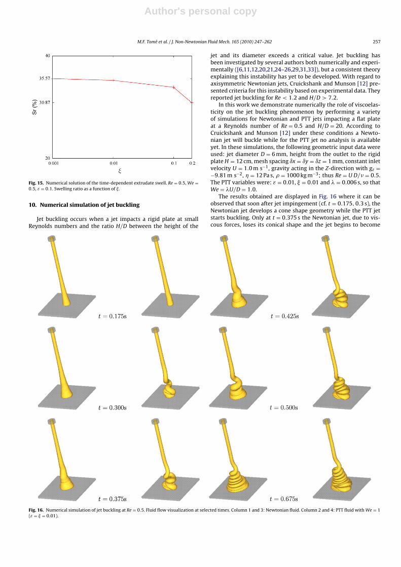
Fig. 15. Numerical solution of the time-dependent extrudate swell. Re = 0.5,We =0.5, ε = 0.1. Swelling ratio as a function of �.

10. Numerical simulation of jet buckling

Jet buckling occurs when a jet impacts a rigid plate at smallReynolds numbers and the ratio H/D between the height of the

jet and its diameter exceeds a critical value. Jet buckling hasbeen investigated by several authors both numerically and experi-mentally ([6,11,12,20,21,24–26,29,31,33]), but a consistent theoryexplaining this instability has yet to be developed. With regard toaxisymmetric Newtonian jets, Cruickshank and Munson [12] pre-sented criteria for this instability based on experimental data. Theyreported jet buckling for Re < 1.2 and H/D > 7.2.

In this work we demonstrate numerically the role of viscoelas-ticity on the jet buckling phenomenon by performing a varietyof simulations for Newtonian and PTT jets impacting a flat plateat a Reynolds number of Re = 0.5 and H/D = 20. According toCruickshank and Munson [12] under these conditions a Newto-nian jet will buckle while for the PTT jet no analysis is availableyet. In these simulations, the following geometric input data wereused: jet diameter D = 6 mm, height from the outlet to the rigidplateH = 12 cm, mesh spacing ıx = ıy = ız = 1 mm, constant inletvelocity U = 1.0 m s−1, gravity acting in the Z-direction with gz =−9.81 m s−2, � = 12 Pa s, � = 1000 kg m−3; thus Re = U D/� = 0.5.The PTT variables were: ε = 0.01, � = 0.01 and � = 0.006 s, so thatWe = �U/D = 1.0.

The results obtained are displayed in Fig. 16 where it can beobserved that soon after jet impingement (cf. t = 0.175,0.3 s), theNewtonian jet develops a cone shape geometry while the PTT jetstarts buckling. Only at t = 0.375 s the Newtonian jet, due to vis-cous forces, loses its conical shape and the jet begins to become

Fig. 16. Numerical simulation of jet buckling at Re = 0.5. Fluid flow visualization at selected times. Column 1 and 3: Newtonian fluid. Column 2 and 4: PTT fluid withWe = 1(ε = � = 0.01).



Fig. 17. Numerical simulation of a jet flowing onto a rigid surface. Fluid flow visualization at selected times. First column: Newtonian jet with Re = 1.5; Second column: PTTjet with Re = 1.5,We = 10 and ε = � = 0.8; Third column: PTT jet with Re = 1.5,We = 10 and ε = � = 0.01.

unstable. At subsequent times it is clear that the Newtonian jetalso undergoes buckling and we can see that at time t = 0.675 sboth jets present the coiling effect.

10.1. The effect of the ε and � parameters on jet buckling

The results obtained in Sections 9 and 9.1 for the extrudate swellshowed that although the value of We was large, depending onthe values selected for ε and �, the viscoelastic effects may not betoo pronounced. A similar situation is observed in the jet bucklingflow and to further demonstrate this fact we have performed threeadditional simulations of a jet flowing onto a rigid surface. The firstsimulation, illustrated in Fig. 17 shows a Newtonian jet impingingon a rigid surface with a Reynolds number ofRe = 1.5 andH/D = 20(U = 1 m s−1, D = 0.006 m, H = 12 cm). The input data used in thisNewtonian simulation were the same as those employed in Section10, except for the lower viscosity of � = 4 Pa s required to produceRe = 1.5. The second simulation considered the same data used inthe first simulation for the PTT model but now with parameters� = 0.06 s, ε = � = 0.8. To show that the parameters ε and � canaffect this problem, a third simulation using ε = � = 0.01 was per-formed (the other input data were kept unchanged). Therefore, inthese two PTT simulations we had Re = 1.5 andWe = 10, but thesetwo non-dimensional numbers were based on zero shear rate fluidproperties. As shown in Fig. 17, the differences between the resultsof these two PTT fluid simulations are dramatic. Indeed, accord-ing to Cruickshank’s predictions the Newtonian jet did not presentthe buckling phenomenon and this is confirmed in our predictionswhere the jet flows smoothly in the radial direction. However,

although the zero shear rate Weissenberg number is quite high(We = 10), the results from the simulation using ε = � = 0.8 displaya flow behaviour similar to the Newtonian case while the simula-tion with ε = � = 0.01 shows that the jet has buckled. Presumably,this happened because of the increase of the extensional viscos-ity after the jet impinged on the solid surface which made the jetmore viscous inhibiting the flow in the radial direction. This facthas been confirmed for two-dimensional PTT jets (see Paulo et al.[21]). These results demonstrate that if the values of parameters εand � are large then the effect of viscoelasticity is diminished, asillustrated in the rheology plots of Fig. 7.

11. Conclusions

This paper presented a finite difference technique for solv-ing three-dimensional free surface flows described by thePhan-Thien–Tanner constitutive equation. The numerical methoddescribed herein used a Marker-and-Cell approach to model thefluid and an accurate approximation of the free surface stress con-ditions was employed. The numerical method developed in thiswork was included into the Freeflow3D simulation system [9]extending Freeflow3D to viscoelastic flows described by PTT flu-ids. The flow in a three-dimensional pipe was simulated and thenumerical results were compared with the corresponding analyticsolutions. The agreement between the two solutions was good andmesh refinement demonstrated the convergence of the numeri-cal technique. Numerical results for the transient extrudate swelland jet buckling were presented and included an investigation ofthe effects of the parameters ε and � on these flows. It was found



that these parameters have a strong effect on these flows. Theextrudate swell was studied for Weissenberg numbers in the range[0, 1] but depending on the parameters ε and �, converged solu-tions can be obtained at higher We. In contrast, for the jet bucklingflow, an upper limit in the Weissenberg number was not observed.The numerical technique presented in this paper proved capableof simulating fully three-dimensional unsteady free surface flowsgoverned by the PTT constitutive equation. However, it has somelimitations that have to be addressed in the future. It is the caseof the momentum equations which are solved explicitly, there-fore imposing a restriction on the time-step size and consequently,realistic simulations can take many hours of CPU time. The simula-tions presented in this paper were performed on a computer with16GB memory, processor Intel Xeon E5345 of 2.33 GHz. One singlesimulation of the extrudate swell took about 70 h while one simu-lation of jet buckling took an average of 50 h. Therefore, an implicitmethod for solving the momentum equations and the paralleliza-tion of the code would result in large gains, a code improvement tobe undertaken in the future.

Acknowledgments

We gratefully acknowledge the support from the Brazilianfunding agencies: FAPESP - Fundacão de Amparo a pesquisa doEstado de São Paulo (project No. 04/16064–9), CNPq - ConselhoNacional de Desenvolvimento Científico e Tecnológico (grantsNos. 304422/2007-0, 470764/2007-4) and CAPES/GRICES grant No.136/5. FTP and MAA acknowledge the funding by GRICES/CAPESproject number 4.1.3(CAPES/CPLP) and by FCT through projectsPTDC/EQU-FTT/71800/2006 and PTDC/EQU-FTT/70727/2006.

Appendix A.

A.1. Calculation of the non-Newtonian tensor on rigid boundaries

To obtain expressions for the components of the non-Newtonianstress tensor on rigid boundaries we extend the accurate methodol-ogy employed in the two-dimensional case (see Paulo et al. [21]) tothe three-dimensional case. The components of the non-Newtoniantensor on rigid boundaries are calculated from Eq. (10) (presentedin Section 4) which we assume to hold with the initial conditionSij = 0. From Eq. (10) we obtain

∂Sij∂t

= −�Re e−t

We SkkSij −∂(uk Sij)

∂xk+ Sjk

(∂ui∂xk

− � Dik)

+Sik(∂uj∂xk

− � Djk)

− 2� SkkDij −2Ree

t

We

{∂Dij∂t

+ ∂(uk Dij)

∂xk

−Djk(∂ui∂xk

− � Dik)

− Dik(∂uj∂xk

− � Djk)} (A.1)

Eq. (A.1) is solved on rigid boundaries parallel to the xy-plane;rigid boundaries parallel to the xz-plane and rigid boundaries par-allel to the yz-plane as follows.

A plane normal to coordinate n has two tangential directions ut1and ut2 . From the no-slip condition we have

∂

∂xt1= ∂

∂xt2= 0 ⇒ ∂un

∂xn= 0

(from continuity and no summation on n). (A.2)

Thus, only the derivatives ∂ui/∂xj with i = t1, t2 and j = n are notzero.

Expansion of Eq. (A.1) and application of these conditions leadsto a set of simplified equations. This set represents a (6 × 6)-nonlinear system for the unknowns Sij . This nonlinear system mustbe calculated on all rigid boundaries for each computational cell.

However, the termRe e−(t/We), which multiplies the nonlinear termsis usually considerably less than unity in which case the corre-sponding nonlinear terms of Eq. (A.1) may be neglected. Hence,at the cells lying at rigid boundaries Eq. (A.3) is solved after simpli-fication with the above no-slip condition

∂Sij∂t

= +Sjk(∂ui∂xk

− � Dik)

+ Sik(∂uj∂xk

− � Djk)

− 2� SkkDij

− 2Ree

t

We

{∂Dij∂t

− Djk(∂ui∂xk

− � Dik)

− Dik(∂uj∂xk

− � Djk)} (A.3)

By making t1 = x, t2 = y and n = z, the simplified form of Eq. (A.3)can be solved for Sij by integrating it over the interval [t, t + ıt].

In general form, the integrals, such as∫ t+ıt

t

(∂V

∂zSlm)

(x, y, z, s) ds,

are approximated by the trapezoidal rule, namely∫ t+ıt

t

(∂V

∂zSlm)

(x, y, z, s)ds

= ıt

2

[(∂V

∂zSlm)

(x, y, z, t) +(∂V

∂zSlm)

(x, y, z, t + ıt)],

where V denotes either u or v while l and m denotes either x, y or z.

Integrals like∫ t+ıtt

e(1/We)s(∂V(x, y, z, s)/∂z)ds are solved by themean value theorem, namely∫ t+ıt

t

e1We s∂V(x, y, z, s)

∂zds = e 1

We t(e1We ıt − 1)We

∂V(x, y, z, t∗)∂z

,

where t∗ ∈ [t, t + ıt], while integrals such as∫ t+ıtt

e(1/We)s∂/∂s(∂V(x, y, z, s)/∂z

)ds are calculated using integration by parts,

∫ t+ıt

t

e1We s

∂

∂s

(∂V(x, y, z, s)

∂z

)ds

= e 1We t

[e

1We ıt

∂V(x, y, z, t + ıt)∂z

− ∂V(x, y, z, t)∂z

− (e1We ıt − 1)

∂V(x, y, z, t∗)∂z

],

where

∂V(x, y, z, t∗)∂z

= 12

[∂V(x, y, z, t)

∂z+ ∂V(x, y, z, t + ıt)

∂z

].

Thus, integrating the simplified form of Eq. (A.3) over the inter-val [t, t + ıt] we get,

S(n+1)ij

= Sij +ıt

2

[Sjk

(∂ui∂xk

− � Dik)

+ Sik(∂uj∂xk

− � Djk)

+S(n+1)jk

(∂u(n+1)i

∂xk− � D(n+1)

ik

)+ S(n+1)

ik

(∂u(n+1)j

∂xk− � D(n+1)

jk

)]−ıt �(SjkDij + S(n+1)

jkD(n+1)ij

)

−2We

Ree

t

We (eıt − 1)

{−Djk

(∂ui(t∗)∂xk

− � Dik(t∗)

)−Dik

(∂uj(t∗)

∂xk− � Djk(t∗)

)}− 2Ree

t

We [eıt

We D(n+1)ij

− Dij − (eıt

We − 1)Dij(t∗)]

(A.4)

where t∗ ∈ [t, t + ıt].



Eq. (A.4) represents a (6 × 6)-linear system for the componentsS(n+1)ij

. By multiplying it by the factor e−(t+ıt/We) we obtain an

expression for the components of S(n+1)ij

as follows:

S(n+1)ij

= e−ıt

We Sij +ıt

2

{e

−ıt

We

[Sjk

(∂ui∂xk

− � Dik)

+ Sik(∂uj∂xk

− � Djk)]

+S(n+1)jk

(∂u(n+1)i

∂xk− � D(n+1)

ik

)+ S(n+1)

ik

(∂u(n+1)j

∂xk− � D(n+1)

jk

)}

−ıt � [e−ıt

We SkkDij + S(n+1)kk

D(n+1)ij

]

−2We

Re(1 − e−

ıt

We )

{−Djk(t∗)

(∂ui(t∗)∂xk

− � Dik(t∗)

)−Dik(t∗)

(∂uj(t∗)

∂xk− � Djk(t∗)

)}− 2Re

[D(n+1)ij

− e−ıt

We Dij − (1 − e−ıt

We )Dij(t∗)].

(A.5)

To solve this system of equations we expand (A.5) and substitutethe equations of Sxx, Syy, Szz and Sxy into the equations for Sxz andSyz . In this case we obtain the following (2 × 2)-linear system forthe unknowns Sxz (n+1) and Syz (n+1){a1X + b1Y = c1a2X + b2Y = c2

(A.6)

where X = Sxz (n+1) and Y = Syz (n+1). The coefficients a1, b1 and c1are given by

a1 = 1 +[�(2 − �) + 2ε(1 − �)

](ıt2

)2(∂u(n+1)

∂z

)2

+ (2 − �) �4

(ıt

2

)2(∂v(n+1)

∂z

)2

b1 =[

3�4

(2 − �) + ε(2 − �) − ε�](

ıt

2

)2∂u(n+1)

∂z

∂v(n+1)

∂z

c1 = e− 1We ıt

{Sxz − Cıt

2∂u(n+1)

∂z

[Sxx + (2 − �)

(ıt

2∂u

∂zSxz

+WeRe

(e1We ıt − 1)

(∂u(t∗)∂z

)2)]

+ (1 − C)ıt

2∂u(n+1)

∂z[Szz

−�(ıt

2∂u

∂zSxz + ıt

2∂v∂zSyz + We

Re(e

1Weıt − 1)

((∂u(t∗)∂z

)2

− �2ıt

2∂v(n+1)

∂z

[Sxy +

(∂v(t∗)∂z

)2))]

+ (2 − �)(ıt

4∂u

∂zSyz

+ıt4∂v∂zSxz+We

Re(e

1Weıt − 1)

∂u(t∗)∂z

∂v(t∗)∂z

)]−εıt

2∂u(n+1)

∂z

[Syy

+(2 − �)(ıt

2∂v∂zSyz + We

Re(e

1Weıt − 1)

(∂v(t∗)∂z

)2)]

− �2ıt

2∂u

∂zSxx − �

2ıt

2∂v∂zSxz + (2 − �)ıt

4∂u

∂zSzz

−εıt2∂u

∂z(Sxx + Syy + Szz)

− 1Re

⎡⎣e ıtWe ∂u(n+1)

∂z− ∂u

∂z− (e

ıt

We − 1)∂u(t∗)∂z

⎤⎦⎫⎬⎭

where C = ((�/2) + ε). The expressions for a2, b2, c2 are similar toa1, b1, c1. The solution of Eq. the (A.6) is given by

Sxz(n+1) =

(c1a1

− b1

a1

(a2c1 − a1c2)(a2b1 − a1b2)

)(A.7)

Syz(n+1) =

((a2c1 − a1c2)(a2b1 − a1b2)

)(A.8)

since of course a1 /= 0 and (a2b1 − a1b2) /= 0.Once Syz (n+1) and Sxz (n+1) have been computed, the other com-

ponents of the non-Newtonian tensor Sij can be calculated from Eq.(A.5).

Appendix B.

In this section we present the equations for calculating the non-Newtonian tensor Sij on rigid boundaries which are parallel to thexy-plane. The equations for obtaining the tensor Sij on rigid bound-aries parallel to the xz- and yz-planes are obtained in the samemanner and therefore they are not given here.

B.1. Boundary cells having only the bottom (or top) facecontiguous with an interior cell face

Rigid boundaries parallel to the xy-plane are identified byboundary cells with the top (or bottom) face in contact with an inte-rior cell face (F or S cell). The values of Sxx, Syy, Szz , Sxy, Sxz and Syz atthe centre of boundary cells are calculated from equations derivedin Section A.1. For instance, if we consider Fig. B.1, then the non-Newtonian tensor Sij at cell centres is obtained as follows. First, wediscretize Eqs. (A.7), (A.8) and (A.5) to calculate an approximationfor Sij on the top face (i, j, k + 1

2 ) of a cell as follows.

Sxx(n+1)

i,j,k+ 12

= e− 1We

ıtSxxi,j,k+ 1

2

+ (2 − �) ıt2

[e−

1We

ıt(∂u

∂zSxz

)∣∣∣i,j,k+ 1

2

+(∂u(n+1)

∂zSxz

(n+1))∣∣∣

i,j,k+ 12

]+ (2 − �)We

Re(1 − e 1

Weıt)

[∂u(t∗)∂z

∣∣∣i,j,k+ 1

2

]2

,

(B.1)

Fig. B.1. Boundary cell with the top face contiguous with an interior cell face.



Syy (n+1)

i,j,k+ 12

= e− 1WeıtSyy

i,j,k+ 12

+ (2 − �) ıt2

[e−

1Weıt

(∂v∂zSyz

)∣∣∣i,j,k+ 1

2

+(∂v(n+1)

∂zSyz

(n+1)

)∣∣∣i,j,k+ 1

2

]+ (2 − �)We

Re(1 − e 1

Weıt )

(∂v(t∗)∂z

∣∣∣i,j,k+ 1

2

)2

,

(B.2)

Szz (n+1)

i,j,k+ 12

= e−1We

ıtSzzi,j,k+ 1

2

− � ıt2

[e−

1Weıt

(∂u

∂zSxz

)∣∣∣i,j,k+ 1

2

+(∂u(n+1)

∂zSxz

(n+1)

)∣∣∣i,j,k+ 1

2

]− � ıt

2

[e−

1Weıt

(∂v∂zSyz

)∣∣∣i,j,k+ 1

2

+(∂v(n+1)

∂zSyz

(n+1)

)∣∣∣i,j,k+

12

]− �We

Re(1 − e 1

Weıt )

[(∂u(t∗)∂z

∣∣∣i,j,k+ 1

2

)2

+(∂v(t∗)∂z

∣∣∣i,j,k+ 1

2

)2],

(B.3)

Sxy (n+1)

i,j,k+ 12

= e− 1WeıtSxy

i,j,k+ 12

+(

1 − �

2

)ıt

2

[e−

1Weıt

(∂u

∂zSyz

)i,j,k+ 1

2

+(∂u(n+1)

∂zSyz

(n+1)

)i,j,k+ 1

2

]+(

1 − �

2

)ıt

2

[e−

1Weıt

(∂v∂zSxz

)i,j,k+ 1

2

+(∂v(n+1)

∂zSxz

(n+1)

)i,j,k+ 1

2

]+(2 − �)We

Re(1 − e 1

Weıt)∂u(t∗)∂z

∣∣∣i,j,k+ 1

2

∂v(t∗)∂z

∣∣∣i,j,k+ 1

2

,

(B.4)

Sxz (n+1)i,j,k+ 1

2=(c1a1

− b1

a1

(a2c1 − a1c2)(a2b1 − a1b2)

)∣∣∣i,j,k+ 1

2

(B.5)

Syz (n+1)i,j,k+ 1

2=(

(a2c1 − a1c2)(a2b1 − a1b2)

)∣∣∣i,j,k+ 1

2

(B.6)

since of course a1|i,j,k+(1/2) /= 0 and (a2b1 − a1b2)|i,j,k+(1/2) /= 0. Theconstants a1, b1, c1, a2, b2 and c2 have been defined in Section A.1.

The values of (∂u(t∗)/∂z)|i,j,k+(1/2) and (∂v(t∗)/∂z)|i,j,k+(1/2) areobtained by averaging between times tn and tn+1, namely

∂u(t∗)∂z

∣∣∣∣i,j,k+ 1

2

= 12

[∂u

∂z

∣∣∣∣i,j,k+ 1

2

+ ∂u(n+1)

∂z

∣∣∣∣i,j,k+ 1

2

],

∂v(t∗)∂z

∣∣∣∣i,j,k+ 1

2

= 12

[∂v∂z

∣∣∣∣i,j,k+ 1

2

+ ∂v(n+1)

∂z

∣∣∣∣i,j,k+ 1

2

],

and the spatial derivatives are approximated by

∂u

∂z

∣∣∣∣i,j,k+ 1

2

=uni,j,k+1−un

i,j,k+12

ız/2,

∂u(n+1)

∂y

∣∣∣∣i,j,k+ 1

2

=u(n+1)i,j,k+1−u(n+1)

i,j,k+ 12

ız/2,

∂v∂z

∣∣∣∣i,j,k+ 1

2

=vni,j,k+1 − vn

i,j,k+ 12

ız2

,∂v(n+1)

∂z

∣∣∣∣i,j,k+ 1

2

=v(n+1)i,j,k+1 − v(n+1)

i,j,k+ 12

ız2

.

The velocities at (i, j, k + 1) are given by

ui,j,k+1 =ui+ 1

2 ,j,k+1+ui− 12 ,j,k+1

2and vi,j,k+1 =

vi,j+ 12 ,k+1 + vi,j− 1

2 ,k+1

2,

respectively. Finally, the values of Sxxi,j,k

, Syyi,j,k

, Szzi,j,k

, Sxyi,j,k

, Sxzi,j,k

and

Syzi,j,k

are obtained using linear interpolation between the nodes(i, j, k + (1/2)) and (i, j, k + 1).

References

[1] M.A. Alves, F.T. Pinho, P.J. Oliveira, Study of steady pipe and channel flows ofa single-mode Phan-Thien–Tanner fluid, J. Non-Newtonian Fluid Mech. 101(2001) 55–76.

[2] M.A. Alves, P.J. Oliveira, F.T. Pinho, A convergent and universally bounded inter-polation scheme for the treatment of advection, Int. J. Numer. Meth. Fluids 41(2003) 47–75.

[3] M.A. Alves, P.J. Oliveira, F.T. Pinho, Benchmark solutions for the flow of Oldroyd-b and PTT fluids in planar contractions, J. Non-Newtonian Fluid Mech. 110(2003) 45–75.

[4] M.A. Alves, F.T. Pinho, P.J. Oliveira, Viscoleastic flow in a 3D Square/squarecontraction, J. Rheol. 52 (2003) 1347–1368.

[5] G.K. Batchelor, An Introduction of Fluid Dynamics, Cambridge University Press,Cambridge, 1967.

[6] A. Bonito, M. Picasso, M. Laso, Numerical simulation of 3d viscoelastic flowswith free surfaces, J. Comput. Phys. 215 (2006) 691–716.

[7] D. Bousfield, R. Keunings, M. Denn, Transient deformation of an inviscid inclu-sion in a viscoelastic extensional flow, J. Non-Newtonian Fluid Mech. 27 (1988)205–221.

[8] D. Bousfield, R. Keunings, G. Marruci, M. Denn, Nonlinear analysis of the surfacetension driven breakup of viscoelastic filaments, J. Non-Newtonian Fluid Mech.21 (1986) 79–97.

[9] A. Castelo, M.F. Tomé, C.N.L. César, S. McKee, J.A. Cuminato, Freeflow: an inte-grated simulation system for three-dimensional free surface flows, J. Comput.Visual. Sci. 2 (2000) 199–210.

[10] M.J. Crochet, R. Keunings, Finite element analysis of die-swell of a highly elasticfluid, J. Non-Newtonian Fluid Mech. 10 (1982) 339–356.

[11] J.O. Cruickshank, Low-Reynolds-number instabilities in stagnating jet flows, J.Fluid Mech. 193 (1988) 111–127.

[12] J.O. Cruickshank, B.R. Munson, Viscous-fluid buckling of plane axisymmetricjets, J. Fluid Mech. 113 (1981) 221–239.

[13] F.H. Harlow, J.E. Welch, The MAC method, Phys. Fluids 8 (1965) 2182–2189.[14] R. Keunings, An algorithm for the simulation of transient viscoelastic flows with

free surfaces, J. Comput. Phys. 62 (1986) 199–220.[15] R. Keunings, D. Bousfield, Analysis of surface tension driven leveling in hori-

zontal viscoelastic films, J. Non-Newtonian Fluid Mech. 22 (1987) 219–233.[16] J.M. Marchal, M.J. Crochet, A new mixed finite element for calculating viscoelas-

tic flow, J. Non-Newtonian Fluid Mech. 26 (1987) 77–114.[17] G. Mompean, M. Deville, Unsteady finite volume of Oldroyd-B fluid through a

three-dimensional planar contraction, J. Non-Newtonian Fluid Mech. 72 (1997)253–279.

[18] P.J. Oliveira, F.T. Pinho, Analytical solution for fully developed channel and pipeflow of Phan-Thien–Tanner fluids, J. Fluid Mech. 387 (1999) 271–280.

[19] G.S. Paulo, Solucão numérica do modelo PTT para escoamentos incompressíveiscom superfícies livres, Ph.D. thesis, ICMC/USP, 2006 (in Portuguese).

[20] G.S. Paulo, M.F. Tomé J.A. Cuminato, A. Castelo, Exact solution of the SPTT modelfor fully developed channel flows, Proceedings of COBEM 2005 (Ouro Preto -MG), CD-ROM, 2005.

[21] G.S. Paulo, M.F. Tomé, S. McKee, A marker-and-cell approach to viscoelastic freesurface flows using the PTT model, J. Non-Newtonian Fluid Mech. 147 (2007)149–174.

[22] N. Phan-Thien, R.I. Tanner, A new constitutive equation derived from networktheory, J. Non-Newtonian Fluid Mech. 2 (1977) 353–365.

[23] D. Rajagopalan, R.C. Armstrong, R.A. Brown, Finite element methods for calcula-tion of steady viscoelastic flow using constitutive equations with a Newtonianviscosity, J. Non-Newtonian Fluid Mech. 36 (1990) 159–192.

[24] N.M. Ribe, A general theory of the dynamics of thin viscous sheets, J. Fluid Mech.457 (2002) 255–283.

[25] N.M. Ribe, Periodic folding of viscous jets, Phys. Rev. E 68 (2003), Art. No. 036305Part 2.

[26] N.M. Ribe, Coiling of viscous jets, Proc. R. Soc. Lond. Series A - Math. Phys. Eng.Sci. 460 (2004) 3223–3239.

[27] M.E. Ryan, A. Dutta, A finite difference simulation of extrudate swell, in:Proceedings of Second World Congress of Chemical Engineering, 1981, pp.277–281.

[28] R.I. Tanner, A theory of die-swell, J. Pol. Sci. 8 (1970) 2067–2078.[29] M.F. Tomé, L. Grossi, A. Castelo, J.A. Cuminato, N. Mangiavacchi, V.G. Ferreira,

F.S. Sousa, S. McKee, A numerical method for solving three-dimensional gener-alized Newtonian free surface flows, J. Non-Newtonian Fluid Mech. 123 (2004)85–103.

[30] M.F. Tomé, A. Castelo, J.A. Cuminato, N. Mangiavacchi, S. McKee, GENSMAC3D:a numerical method for solving unsteady three-dimensional free surface flows,Int. J. Numer. Meth. Fluids 37 (2001) 747–796.

[31] M.F. Tomé, A. Castelo, V.G. Ferreira, S. McKee, A finite difference techniquefor solving the Oldroyd-B model for 3D-unsteady free surface flows, J. Non-Newtonian Fluid Mech. 154 (2008) 179–206.

[32] M.F. Tomé, B. Duffy, S. McKee, A numerical technique for solving unsteadynon-Newtonian free surface flows, J. Non-Newtonian Fluid Mech. 62 (1996)9–34.



[33] M.F. Tomé, N. Mangiavacchi, A. Castelo, J.A. Cuminato, S. McKee, A finite dif-ference technique for simulating unsteady viscoelastic free surface flows, J.Non-Newtonian Fluid Mech. 106 (2002) 61–106.

[34] M.F. Tomé, S. McKee, GENSMAC: a computational marker-and-cell methodfor free surface flows in general domains, J. Comput. Phys. 110 (1994)171–186.

[35] S. Xue, N. Phan-Thien, R.I. Tanner, Numerical study of secondary flows ofviscoelastic fluid in straight pipes by an implicit finite volume method, J. Non-Newtonian Fluid Mech. 59 (1995) 191–213.

[36] S. Xue, N. Phan-Thien, R.I. Tanner, Numerical study of secondary flows ofviscoelastic fluid in straight pipes by an implicit finite volume method, J. Non-Newtonian Fluid Mech. 74 (1998) 195–245.

Documents

Author's personal copy - Faculdade de Engenharia da