Embed Size (px)
Citation preview

http://www.jstor.org
Economic Growth and the EnvironmentAuthor(s): Gene M. Grossman and Alan B. KruegerSource: The Quarterly Journal of Economics, Vol. 110, No. 2, (May, 1995), pp. 353-377Published by: The MIT PressStable URL: http://www.jstor.org/stable/2118443Accessed: 19/08/2008 07:17
Your use of the JSTOR archive indicates your acceptance of JSTOR's Terms and Conditions of Use, available at
http://www.jstor.org/page/info/about/policies/terms.jsp. JSTOR's Terms and Conditions of Use provides, in part, that unless
you have obtained prior permission, you may not download an entire issue of a journal or multiple copies of articles, and you
may use content in the JSTOR archive only for your personal, non-commercial use.
Please contact the publisher regarding any further use of this work. Publisher contact information may be obtained at
http://www.jstor.org/action/showPublisher?publisherCode=mitpress.
Each copy of any part of a JSTOR transmission must contain the same copyright notice that appears on the screen or printed
page of such transmission.
JSTOR is a not-for-profit organization founded in 1995 to build trusted digital archives for scholarship. We work with the
scholarly community to preserve their work and the materials they rely upon, and to build a common research platform that
promotes the discovery and use of these resources. For more information about JSTOR, please contact [email protected].

ECONOMIC GROWTH AND THE ENVIRONMENT*
GENE M. GROSSMAN AND ALAN B. KRUEGER
We examine the reduced-form relationship between per capita income and various environmental indicators. Our study covers four types of indicators: urban air pollution, the state of the oxygen regime in river basins, fecal contamination of ri'ver basins, and contamination of river basins by heavy metals. We find no evidence that environmental quality deteriorates steadily with economic growth. Rather, for most indicators, economic growth brings an initial phase of deterioration followed by a subsequent phase of improvement. The turning points for the different pollutants vary, but in most cases they come before a country reaches a per capita income of $8000.
I. INTRODUCTION
Will continued economic growth bring ever greater harm to the earth's environment? Or do increases in income and wealth sow the seeds for the amelioration of ecological problems? The answers to these questions are critical for the design of appropriate development strategies for lesser developed countries.
Exhaustible and renewable natural resources serve as inputs into the production of many goods and services. If the composition of output and the methods of production were immutable, then damage to the environment would be inextricably linked to the scale of global economic activity. But substantial evidence suggests that development gives rise to a structural transformation in what an economy produces (see Syrquin [1989]). And societies have shown remarkable ingenuity in harnessing new technologies to conserve scarce resources. In principle, the forces leading to change in the composition and techniques of production may be suffi- ciently strong to more than offset the adverse effects of increased economic activity on the environment. In this paper we address this empirical issue using panel data on ambient pollution levels in many countries.
Examination of the empirical relationship between national income and measures of environmental quality began with our
*We thank the Ford Foundation, the Sloan Foundation, the John S. Guggen- heim Memorial Foundation, the Institute for Policy Reform, and the Centers of International Studies and of Economic Policy Studies at Princeton University for financial support. We are grateful to Peter Jaffee, who tutored us on the various dimensions of water quality, to Robert Bisson, who provided us with the GEMS/ Water data, and to seminar participants at the O.E.C.D. Development Centre and the Institute for International Economic Studies in Stockholm, Sweden, who gave us helpful comments and suggestions. Special thanks go to James Laity, whose research assistance was simply extraordinary.
? 1995 by the President and Fellows of Harvard College and the Massachusetts Institute of Technology. The Quarterly Journal of Economics, May 1995
354 QUARTERLY JOURNAL OF ECONOMICS
paper on the likely environmental impacts of a North American Free Trade Agreement [Grossman and Krueger 1993]. There we estimated reduced-form regression models relating three indica- tors of urban air pollution to characteristics of the site and city where pollution was being monitored and to the national income of the country in which the city was located. Selten and Song [1992] and Holtz-Eakin and Selden [1992] have used similar methods to relate estimated rates of emission of several air pollutants (with estimates formed by multiplying the aggregate national consump- tion of each of several fuel types by technical coefficients that are meant to reflect contemporaneous abatement practices in each country) to the national income level of the emitting country. The World Bank Development Report [1992] also reports evidence on the relationship between several measures of environmental qual- ity and levels of national GDP.1 These studies tend to find that environmental degradation and income have an inverted U-shaped relationship, with pollution increasing with income at low levels of income and decreasing with income at high levels of income.
The main contribution of the present paper is that it employs reliable data and a common methodology to investigate the relation- ship between the scale of economic activity and environmental quality for a broad set of environmental indicators. We attempt to include in our study all of the dimensions of environmental quality for which actual measurements have been taken by comparable methods in a variety of countries. To this end, we use all of the available panel data in the Global Environmental Monitoring System's (GEMS) tracking of urban air quality in different cities in the developed and developing world. And we use much of the panel data from the GEMS monitoring of water quality in river basins around the globe. Although these measures are far from a compre- hensive list of all relevant variables describing the state of the ecosystem, the variety in the types of pollutants included in our investigation may allow generalization (with caveats) to some other types of environmental problems, and it is more comprehen- sive than that used in previous studies.
1. The report includes estimates of the relationship between income and the percentage of the population without access to safe water or urban sanitation, using internal World Bank data, and on the relationship between income and municipal solid waste per capita, using O.E.C.D. and World Resources Institute estimates for 39 countries complied for the year 1985. A background study for this report (see Shafik and Bandyopadhyay [1992]) also examined total and annual deforestation between 1961 and 1986 for samples of 77 and 66 countries, respectively, plus two of the water-quality indicators studied here.
ECONOMIC GROWTH AND THE ENVIRONMENT 355
In the next section we describe the environmental indicators and the sources of our data. We discuss briefly the anthropogenic sources of the various pollutants and the health hazards they pose, and note the forms of environmental degradation that are absent from our study. Section III details the common methodology that we employ in analyzing the cross-national and time-series pollution data. The results of our analysis are presented and discussed in Section IV. The final section discusses the consistency of our findings with those reported by other authors and comments on the lessons to be drawn from them.
II. THE ENVIRONMENTAL INDICATORS
Environmental quality has many dimensions. Our lives are affected by the air we breathe, the water we drink, the beauty we observe in nature, and the diversity of species with which we come into contact. The productivity of our resources in producing goods and services is influenced by climate, rainfall, and the nutrients in the soil. We experience discomfort from excessive noise and crowding, and from the risk of nuclear catastrophe. Each of these dimensions of environmental quality (and others) may respond to economic growth in a different way. Therefore, a study of environ- ment and growth should aim to be as comprehensive as possible.
Unfortunately, a paucity of data limits the scope of any such study. Only in recent years have the various aspects of environmen- tal quality been carefully assessed and only a small number of indicators have been comparably measured in a variety of countries at different stages of development. Comparability and reliability are the central aims of the effort spearheaded by GEMS, a joint project of the World Health Organization and the United Nations Environmental Programme. For almost two decades GEMS has monitored air and water quality in a cross section of countries. These panel data provide the basis for our research.
The GEMS/Air project monitors air pollution in selected urban areas. Concentrations of sulfur dioxide (SO2) and suspended particulate matter are measured on a daily (or sometimes less frequent) basis; and the raw data are used to calculate the median, eightieth percentile, ninety-fifth percentile, and ninety-eighth per- centile observation in a given year.2 GEMS also reports informa-
2. The GEMS data for 1977-1984 are published by the World Health Organiza- tion in the series Air Quality in Selected Urban Areas. We obtained unpublished data for 1985-1988 from the U. S. Environmental Protection Agency.
356 QUARTERLY JOURNAL OF ECONOMICS
tion about the monitoring stations, including the nature of the land use nearby and the type of the monitoring instrument used. As some of the methods used to measure suspended particulates reflect primarily concentrations of coarser, heavier particles while others capture quantities of finer, lighter particles, and as the different types of particles pose different health risks, we have chosen to divide the sample for suspended particles into two subsamples, one for "heavy particles" and the other for "smoke."
Participation in the GEMS/Air project has varied over time. For SO2, the sample comprised 47 cities in 28 countries in 1977, 52 cities in 32 countries in 1982, and 27 cities in 14 countries in 1988. A total of 42 countries are represented in the sample. Heavy particles were monitored in 21 cities in 11 countries in 1977, 36 cities in 17 countries in 1982, and 26 cities in 13 countries in 1988, with 29 countries represented in all. The sample for smoke included 18 cities in 13 countries in 1977, 13 cities in 9 countries in 1982, and 7 cities in 4 countries in 1988, with a total of 19 countries in all. In all cases, monitoring sites were chosen to be fairly representative of the geographic and economic conditions that exist in different regions of the world [Bennett et al. 1985].
The air quality variables in our study are among the most commonly used indicators of air pollution in cities and other densely populated areas. Sulfur dioxide and suspended particles are found in great quantities in many cities, and their severe effects on human health and the natural environment have long been recognized. Important forms of urban air pollution absent from our sample include nitrogen oxides, carbon monoxide, and lead. Perhaps more important is the omission of the air pollutants that affect the global atmosphere, and specifically those that contribute to ozone depletion and to the greenhouse effect. These would include chlorofluorocarbons (CFC's), carbon dioxide, methane, nitrous oxide, and tropospheric ozone.
Both sulfur dioxide and suspended particulate matter (espe- cially, the finer particles) have been linked to lung damage and other respiratory disease.3 Sulfur dioxide is emitted naturally by volcanoes, decaying organic matter, and sea spray. The major anthropogenic sources include the burning of fossil fuels in electric- ity generation and home heating, and the smelting of nonferrous
3. For example, Lave and Seskin [1970] find that variation in SO2 and population density together explain two-thirds of the variation in death from bronchitis in a sample of U. S. cities. See also Dockery et al. [1993] and U. S. Environmental Protection Agency [1982].
ECONOMIC GROWTH AND THE ENVIRONMENT 357
ores [World Resources Institute 1988]. Automobile exhaust and certain chemical manufacturers are also sources of SO2 in some countries [Kormondy 1989]. Particulates are generated naturally by dust, sea spray, forest fires, and volcanoes. Economic activities responsible for pollution of this sort include certain industrial processes and domestic fuel combustion.
The GEMS/Water project monitors various dimensions of water quality in river basins, lakes, and groundwater aquifers. The number of observations from lake and groundwater stations is, however, too small for any meaningful statistical analysis. There- fore, we focus our attention on the data that describe the state of river basins. In choosing where to locate its monitoring stations, GEMS/Water has given priority to rivers that are major sources of water supply for municipalities, irrigation, livestock, and selected industries. A number of stations were included to monitor interna- tional rivers and rivers discharging into oceans and seas. Again, the project aimed for representative global coverage. The available water data cover the period from 1979 to 1990. By January 1990 the project had the active participation of 287 river stations in 58 different countries. Each such station reports thirteen basic chemi- cal, physical, and microbiological variables, several globally signifi- cant pollutants including various heavy metals and pesticides, and a number of site-specific, optional variables. Information also is provided about the measurement method and frequency of observa- tion, as well as the exact location of the monitoring station.4 Our study makes use of all variables that can be considered indicators of water quality, provided that they have anthropogenic constituents and that at least ten countries are represented in the sample.
We focus on three categories of indicators relating to water quality. First, we examine the state of the oxygen regime. Aquatic life requires dissolved oxygen to metabolize organic carbon. Con- tamination of river water by human sewage or industrial dis- charges (by, for example, pulp and paper mills) increases the concentration of organic carbon in forms usable by bacteria. The more numerous are the bacteria, the greater is the demand for dissolved oxygen, leaving less oxygen for fish and other higher forms of aquatic life. At high levels of contamination the fish population begins to die off. A similar problem can arise when river
4. Summary data are published triennially by the Global Environmental Monitoring System in the series GEMS/Water Data Summary. We obtained raw data from Robert Bisson of the Canada Centre for Inland Waters, which is the WHO Collaborating Centre for Surface and Groundwater Quality.
358 QUARTERLY JOURNAL OF ECONOMICS
water is overenriched by nutrients such as are contained in runoff from agricultural areas where fertilizers are used intensively. Excess nitrogen and phosphorus promote algal growth. The de- cay of dying algae consumes oxygen, which is lost to the fish population.
Some GEMS/Water stations directly monitor the level of dissolved oxygen in a river as an indication of the state of the oxygen regime. Other stations measure instead the contamination by organic compounds as an indication of the competing demands for oxygen. One measure of this, called biological oxygen demand (BOD), is the amount of natural oxidation that occurs in a sample of water in a given period of time. Another measure, called chemical oxygen demand (COD), is the amount of oxygen con- sumed when a chemical oxidant is added to a sample of water. Whereas dissolved oxygen is a direct measure of water quality, BOD and COD are inverse measures, indicating the presence of contaminants that will eventually cause oxygen loss. Some stations measure all three water quality indicators. We investigate the relationship between levels of income and all three of these indicators of the state of the oxygen regime, as well as the concentration of nitrates in the river water.
Pathogenic contamination is our second indicator of water quality. Pathogens in sewage cause a variety of debilitating and sometimes fatal diseases such as gastroenteritis, typhoid, dysen- tery, cholera, hepatitis, schistosomiasis, and giardiasis. The pres- ence of pathogens is not a consequence of economic activity per se, but rather contamination occurs when raw sewage is discharged without adequate treatment. The GEMS/Water project monitors fecal coliform-which are harmless bacteria found in great num- bers in human and animal feces-as an indicator of the presence of the harmful pathogens. The data set includes concentrations of fecal coliform in rivers in 42 different countries. In some cases, GEMS has monitored total coliform instead of (or in addition to) fecal coliform. Total coliform are a broader class of bacteria which, unlike fecal coliform, include some organisms that are found naturally in the environment. For this reason, the concentration of total coliform is considered to be an inferior indicator of fecal contamination. Nonetheless, we estimate the relationship between levels of national income and concentrations of total coliform found in rivers located in 22 countries.
Heavy metals comprise our third category of water pollution. Metals discharged by industry, mining, and agriculture accumulate
ECONOMIC GROWTH AND THE ENVIRONMENT 359
into bottom sediment, which then is released slowly over time. The metals show up in drinking water and bioaccumulate in fish and shellfish that are later ingested by humans. The GEMS/Water project monitors a number of heavy metals (as well as some other toxics), but the sample sizes for some are too small to allow statistical analysis. We examine concentrations of lead, cadmium, arsenic, mercury and nickel, all of which have reasonable numbers of observations from rivers located in at least ten countries. The health risks associated with these particular metals are many: lead causes convulsions, anemia, kidney damage, brain damage, cancer, and birth defects; cadmium is associated with tumors, renal dysfunction, hypertension, and arteriosclerosis; arsenic induces vomiting, poisoning, liver damage, and kidney damage; mercury contributes to irritability, depression, kidney and liver damage, and birth defects; and nickel causes gastrointestinal and central nervous system damage and cancer.
As we have noted, the GEMS data do not cover all dimensions of environmental quality. Besides the air pollutants that affect global atmospheric conditions, important omissions include indus- trial waste, soil degradation, deforestation, and loss of biodiversity. While we view our inability to examine the effects of growth on these forms of environmental damage as unfortunate, we believe that there is much to be learned from studying how the many indicators of air and water quality respond to changes in output levels.
III. METHODOLOGICAL ISSUES
To study the relationship between pollution and growth, we estimate several reduced-form equations that relate the level of pollution in a location (air or water) to a flexible function of the current and lagged income per capita in the country and to other covariates. An alternative to our reduced-form approach would be to model the structural equations relating environmental regula- tions, technology, and industrial composition to GDP, and then to link the level of pollution to the regulations, technology and industrial composition. We think there are two main advantages to a reduced-form approach. First, the reduced-form estimates give us the net effect of a nation's income on pollution. If the structural equations were estimated, one would need to solve back to find the net effect of income changes on pollution, and confidence in the implied estimates would depend upon the precision and potential

360 QUARTERLY JOURNAL OF ECONOMICS
biases of the estimates at every stage. Second, the reduced-form approach spares us from having to collect data on pollution regulations and the state of technology, data which are not readily available and are of questionable validity. A limitation of the reduced-form approach, however, is that it is unclear why the estimated relationship between pollution and income exists. Never- theless, we think that documenting the reduced-form relationship between pollution and income is an important first step.
Specifically, we estimate
(1) Yit = Gito, + GitP2 + Gi3t3 + Git-04 + GUit-45
+ Gi3t6 + Xit'P7 + Eit,
where Yit is a measure of water or air pollution in station i in year t, Git is GDP per capita in year t in the country in which station i is located, Git- is the average GDP per capita over the prior three years, Xit is a vector of other covariates, and fi is an error term. The
O3's are parameters to be estimated. For the air pollutants the dependent variable is defined as the
median daily concentration of the pollutant at each site over the course of the year. The mean values of the air pollutants were not reported. Other percentiles of air pollutants were reported, and our analysis of the ninety-fifth percentile concentrations indicated qualitatively similar results. For the water pollutants we used the mean value of the pollutant over the course of the year as our dependent variable, because median values were omitted whenever there were fewer than four observations above the minimum detectable level of the measuring device.
Except for two pollutants we measure the dependent variables as a concentration level (e.g., Rg per cubic meter). The exceptions are total coliform and fecal coliform, which we measure as log(1 + Y), where Yis the concentration level. The reasons for this transformation are (i) the coliform grow exponentially, (ii) the distribution of the coliform is (highly) positively skewed, and (iii) we cannot take the log of Y in some cases because the level of coliform is reported as zero whenever the reading falls below the minimum detectable level of the measuring device.
The key GDP variable is taken from Summers and Heston [1991], and in principle measures output per capita in relation to a common set of international prices.5 Although our measures of
5. The Summers and Heston data are available only through 1988, whereas the water pollution data are available through 1990. World Bank GDP estimates,
ECONOMIC GROWTH AND THE ENVIRONMENT 361
pollution pertain to specific cities or sites on rivers, GDP is measured at the country level. Since environmental standards are often set at a national level, using country-level GDP per capita (as opposed to local income) is arguably appropriate. Moreover, data on city or river level GDP per capita are not readily available, and are not as comparable across countries as are the Summers and Heston data. We have included a cubic of the average GDP per capita in the preceding three years to proxy the effect of "permanent income" and because past income is likely to be a relevant determinant of current environmental standards. As a practical matter, however, lagged and current GDP per capita are highly correlated, so including just current (or just lagged) GDP per capita does not qualitatively change the results. Experimentation with unre- stricted dummy variables indicating ranges of GDP suggested that the cubic specification is flexible enough to describe the varied relationships between pollution and GDP.
In estimating the relationship between pollution and national income, we adjusted for the year in which the measurement was taken by including a linear time trend as a separate regressor.6 We did so because we did not want to attribute to national income growth any improvements in local environmental quality that might actually be due to global advances in the technology for environmental preservation or to an increased global awareness of the severity of environmental problems.
We included additional covariiates besides income and time to describe characteristics of the site where the monitoring stations were located and to describe the specific method of monitoring. Since these location-specific variables are unlikely to be correlated with national income, their inclusion is not necessary for unbiased estimation of the coefficients of interest. However, by including these additional variables, we are able to reduce the residual variance in the relationship between pollution and income and thus generate more precise estimates. In our estimation using the various measures of urban air pollution, we used dummy variables indicating the location of the monitoring station within the city (central city or suburban) and the nature of the land use nearby the station (industrial, commercial, residential, or unknown). We also
however, are available through 1990. To increase the sample, we used the ratio of the Summers and Heston GDP data to World Bank GDP data in 1988 to index-link the World Bank data in 1989 and 1990.
6. When we experimented by including unrestricted year dummies, the coefficients on them were approximately linear, and the other coefficients were not meaningfully different.
362 QUARTERLY JOURNAL OF ECONOMICS
included the population density of the city, a dummy indicating whether the city is located along a coastline (reflecting the dispersal properties of the local atmosphere), and-for the two types of suspended particles-a dummy indicating whether the city is located within 100 miles of a desert. For pollutants that were measured with different measuring devices at different stations, we included dummies indicating the type of measuring device, to account for the fact that some monitoring devices are more sensitive than others.7
We used a more limited set of covariates for the water pollutants because the data set provided less information about the placement of the monitoring station. In addition to the GDP per capita terms and the time trend, we included the mean annual water temperature in the river in which the monitoring station is located.8 This is a pertinent explanatory variable because, for many pollutants, the rate of dissolution depends on the temperature of the water. Finally, where appropriate, we included dummies indicating the type of measuring device used to monitor the pollutant.
A final methodological issue concerns the appropriate estima- tor of equation (1). If there are any characteristics of the monitor- ing sites that influence pollution but are not included in our list of independent variables, these will induce a temporal correlation in the error term, fit. To account for this, we estimate equation (1) by generalized least squares (GLS). More specifically, we assume the error term is the sum of two components:
Eit= -i + eit)
where cai is a site-specific random component and ci is an idiosyn- cratic error component. We assume that cov (a?,cxj) = 0 and COV (Ei',Ejt) = 0 for i ? j and t ? s. We employ a random-effects estimator that takes into account the unbalanced nature of our panel.
7. All of these variables except population density, location on a coast, and location near a desert, are available in the GEMS data. We derived the other variables by inspecting maps and country almanacs.
8. For about one-third of the observations, we lacked information on the mean annual water temperature. In these cases we imputed temperature values by first running a regression of the mean water temperature on the latitude of the river for the subsample containing mean temperature, and then constructing fitted values using the estimated regression coefficient and the latitude of the river with missing temperature data. In practice we suspect this procedure works well because latitude accounts for over 70 percent of the variation in mean water temperature.
ECONOMIC GROWTH AND THE ENVIRONMENT 363
IV. RESULTS
We have estimated equation (1) for each of the pollutants described in Section II. The GLS estimates are reported in Appendixes 1-4. The tables in these appendixes also show the p-values for the three current income variables, the three lagged income variables, and the six income variables taken together. In view of the strong multicollinearity between current and lagged GDP, as well as among powers of GDP, it is difficult to infer much about the individual coefficients. However, in most cases the collection of current and lagged GDP terms is highly significant. It appears therefore that national income is an important determi- nant of local air and water pollution.
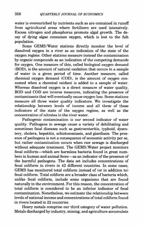
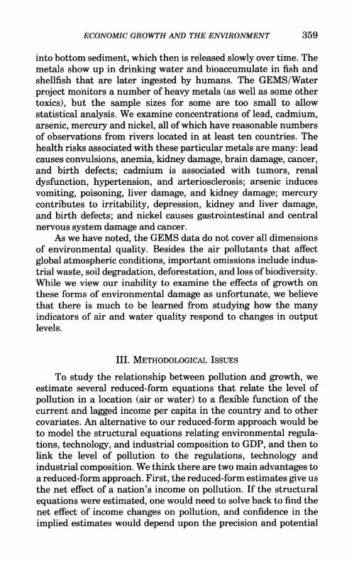
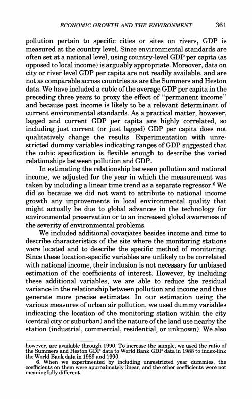
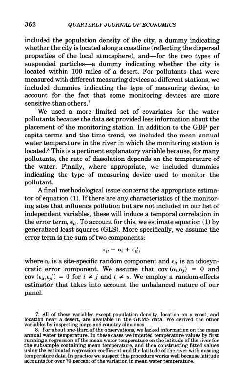
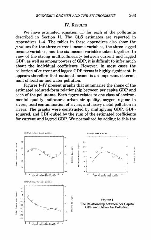
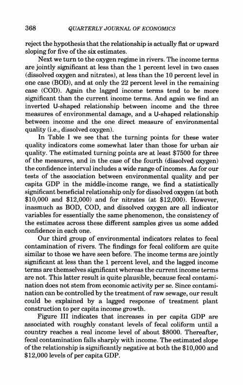
Figures I-IV present graphs that summarize the shape of the estimated reduced-form relationship between per capita GDP and each of the pollutants. Each figure relates to one class of environ- mental quality indicators: urban air quality, oxygen regime in rivers, fecal contamination of rivers, and heavy metal pollution in rivers. The graphs were constructed by multiplying GDP, GDP- squared, and GDP-cubed by the sum of the estimated coefficients for current and lagged GDP. We normalized by adding to this the
GEMS/AIR: Sulphur Dioxide in Cities GEMS/AIR: Smoke in Cities
-2 4
50 -150-
'a ~~~~~ lo * ~~~~~1 3'z
0 l l lOGItq... ..
0 2 A A A 10 12 14 IA... 6 . . .. . 18 0 2 A A 8 10 12 GOP Per Capita (19A5 SIOGOM) GOP Per Capita (1985 $1IG2-s)
GEMS/AIR. Heavy Particles An CAtAes
25~~~~~~~~~~~~~~~~ - I
100~~~~~~~~~~~~~~~~~~~~~0
X -1050 \9 ? -. Th FIGURE I 5
\--I o The ~~~~Relationship between per Capita
-200 GDP and Urban Air Pollution A -250 -2
-~~~~~~~~~~~~~~~~~~~~~~5 -5
0 2 4 6 8 10 12 14 16 18 GOP Per Capita (19M5 S1,OO0s)
364 QUARTERLY JOURNAL OF ECONOMICS
GEMS/WATER: Dissolved Oxygen in Rivers GEMS/WATER: Biological Oxygen Demand in Rivers
-2 -3
6 - L - - ? r 1 3 0~~~~~~~~~~~~~~~~~~6 0 2 2~~~~~~~~~~~~~~~~~~~~0-
-2 E
0 0~~~~~~~~~~- s-
-6 r-2 -20 --1
O 2 4 6 8 TO 12 14 16 18 0 2 4 6 8 10 12 14 16 1A GOP Per Capita (1985 $1,000s) GDP Per Capita t19A5 $1,000s)
GEMS/WATER: Chemical Oxygen Demand in Rivers GEMS/WATER: Nitrates in Rivers
350 - l l l l l l l l l l -3 l l l l l l l l l l -3
,, 300 - 10
20 2 . 8- -2
a 200 A 6
- " 150 X-O 0 o A 2 - A 50 -2c
0 2 A 6 A TO 12 T4 16 TA 0 2 4 6 A TO 12 T4 16 TA GDP Per Capita (1985 $1,000s) GDP Per Capita (1985 51,000s)
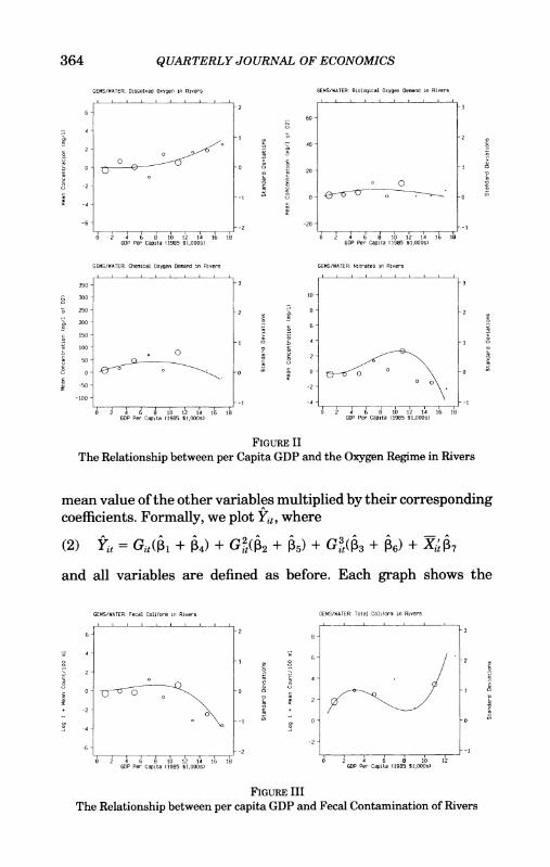
FIGURE II
The Relationship between per Capita GDP and the Oxygen Regime in Rivers
mean value of the other variables multiplied by their corresponding coefficients. Formally, we plot Yj,, where
(2) Yt = G-t(I3 + N) + G (P2 + P5) + G ($3 + I6) + XitAP7
and all variables are defined as before. Each graph shows the
GEMS/WATER: Fecal Coliform in Rivers GEMS/WATER: Total Coliform in Rivers
6- 2 8-
6 2 A 2~~~~~~~~~~~~~~~~~~~~
2 -
0 - 0~~~~~~~A- 0
-G -2 -T~~~~~~~~~~~~~~~~~~~
O 2 A 6 A 10 12 TA 16 TA 0 2 A 6 A 10 12 GDP Per Capita (1985 $T,000s) GDP Per Capita (T985 $ T,000s)
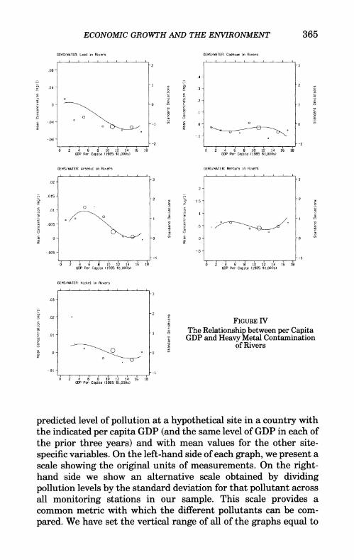
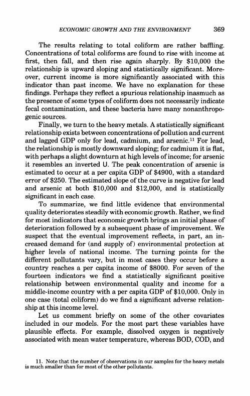
FIGURE III
The Relationship between per capita GDP and Fecal Contamination of Rivers
ECONOMIC GROWTH AND THE ENVIRONMENT 365
GEMS/WATER: Lead in Rivers GEMS/WATER: Cadmium in Rivers
0 .0 41-2 -3
.08 - DtoI -04 -1 0~~~~~~~~~~~~~~~~~~~~~~~. 0
0 2 4 6 8 10 12 14 16 18 0 2 4 6 8 10 12 14 16 18 GOP Per Capita (1985 S1,000s) GOP Per Capita (1985 S1,000s)
GEMS/WATER: Arsenci Rivers GEMS/WATER: MercuryinRvr
33 3
-, ohs
2 , -5 <2 .
0 -
0 -0
-.005-.
l 2 -
0 2 4 6 8 10 12 14 16 18 0 2 4 6 8 10 12 14 16 18 GDP Per Capita (1985 $1,000s) GDP Per Capita (1985 $1,000s)
GEMS/WATER: Nickel in Rivers
- ~ ~ ~ ~ ~ ~ ~ ~ ~ ~ ~ ~ ~ ~~ ~~~~~~~~~~~
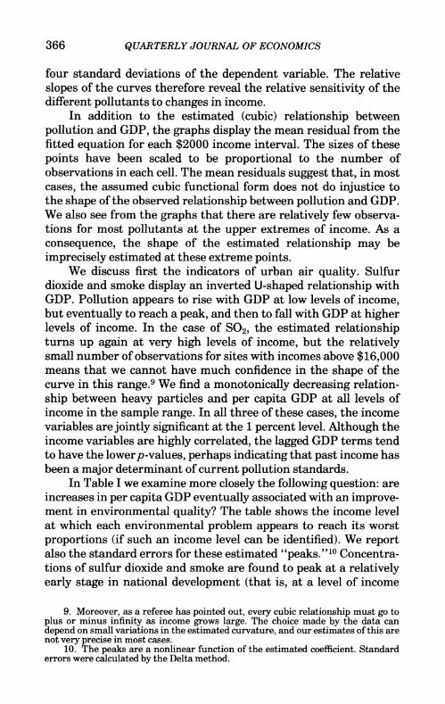
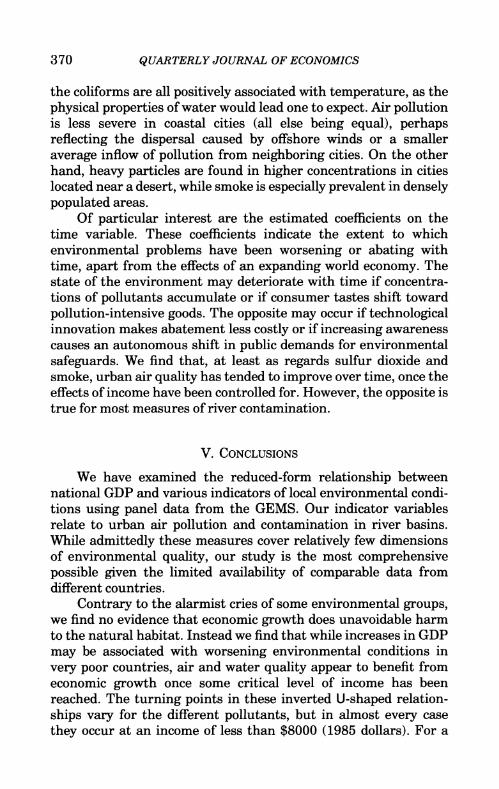
E .02 - . -2 c FIGURER -
X01 The Relationship between per Capita
c 01 - r ~~~~~GDP and Heavy Metal Contamination X
O~~~~ ~~ t) O _O On ~~~of Rivers 0 l0
-01 -1
0 2 4 6 8 10 12 14 16 18 GDP Per Capita (1985 $1,000s)
predicted level of pollution at a hypothetical site in a country with the indicated per capita GDP (and the same level of GDP in each of the prior three years) and with mean values for the other site- specific variables. On the left-hand side of each graph, we present a scale showing the original units of measurements. On the right- hand side we show an alternative scale obtained by dividing pollution levels by the standard deviation for that pollutant across all monitoring stations in our sample. This scale provides a common metric with which the different pollutants can be com- pared. We have set the vertical range of all of the graphs equal to
366 QUARTERLY JOURNAL OF ECONOMICS
four standard deviations of the dependent variable. The relative slopes of the curves therefore reveal the relative sensitivity of the different pollutants to changes in income.
In addition to the estimated (cubic) relationship between pollution and GDP, the graphs display the mean residual from the fitted equation for each $2000 income interval. The sizes of these points have been scaled to be proportional to the number of observations in each cell. The mean residuals suggest that, in most cases, the assumed cubic functional form does not do injustice to the shape of the observed relationship between pollution and GDP. We also see from the graphs that there are relatively few observa- tions for most pollutants at the upper extremes of income. As a consequence, the shape of the estimated relationship may be imprecisely estimated at these extreme points.
We discuss first the indicators of urban air quality. Sulfur dioxide and smoke display an inverted U-shaped relationship with GDP. Pollution appears to rise with GDP at low levels of income, but eventually to reach a peak, and then to fall with GDP at higher levels of income. In the case of SO2, the estimated relationship turns up again at very high levels of income, but the relatively small number of observations for sites with incomes above $16,000 means that we cannot have much confidence in the shape of the curve in this range.9 We find a monotonically decreasing relation- ship between heavy particles and per capita GDP at all levels of income in the sample range. In all three of these cases, the income variables are jointly significant at the 1 percent level. Although the income variables are highly correlated, the lagged GDP terms tend to have the lowerp-values, perhaps indicating that past income has been a major determinant of current pollution standards.
In Table I we examine more closely the following question: are increases in per capita GDP eventually associated with an improve- ment in environmental quality? The table shows the income level at which each environmental problem appears to reach its worst proportions (if such an income level can be identified). We report also the standard errors for these estimated "peaks." 10 Concentra- tions of sulfur dioxide and smoke are found to peak at a relatively early stage in national development (that is, at a level of income
9. Moreover, as a referee has pointed out, every cubic relationship must go to plus or minus infinity as income grows large. The choice made by the data can depend on small variations in the estimated curvature, and our estimates of this are not very precise in most cases.
10. The peaks are a nonlinear function of the estimated coefficient. Standard errors were calculated by the Delta method.
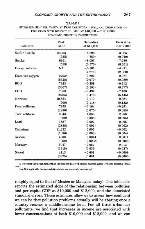
ECONOMIC GROWTH AND THE ENVIRONMENT 367
TABLE I ESTIMATED GDP PER CAPITA AT PEAK POLLUTION LEVEL, AND DERIVATIVES OF
POLLUTION WITH RESPECT TO GDP AT $10,000 AND $12,000 (STANDARD ERRORS IN PARENTHESES)
Peak Derivative Derivative Pollutant GDP at $10,000 at $12,000
Sulfur dioxide $4053 -5.295 -3.065 (355) (.780) (0.910)
Smoke 6151 -8.053 -7.780 (539) (3.570) (8.651)
Heavy particles NA -5.161 -4.811 (2.271) (2.080)
Dissolved oxygen 2703a 0.202 0.277 (5328) (0.070) (0.080)
BOD 7623 -0.358 -0.612 (3307) (0.503) (0.777)
COD 7853 -3.494 -7.106 (2235) (3.470) (5.445)
Nitrates 10,524 0.110 -0.384 (500) (0.118) (0.132)
Fecal coliform 7955 -0.164 -0.391 (1296) (0.075) (0.085)
Total coliform 3043 1.083 2.950 (309) (0.323) (0.895)
Lead 1887 -0.007 -0.005 (2838) (0.002) (0.002)
Cadmium 11,632 0.005 -0.002 (1096) (0.006) (0.004)
Arsenic 4900 -0.0014 -0.0011 (250) (0.0903) (0.0002)
Mercury 5047 -0.057 -0.013 (1315) (0.039) (0.037)
Nickel 4113 -0.001 -0.0009 (3825) (0.001) (0.0006)
a. We report the trough rather than the peak for dissolved oxygen, because higher levels are desirable in this case.
NA: Not applicable (because relationship is monotonically decreasing).
roughly equal to that of Mexico or Malaysia today). The table also reports the estimated slope of the relationship between pollution and per capita GDP at $10,000 and $12,000, and the associated standard errors. These estimates allow us to assess how confident we can be that pollution problems actually will be abating once a country reaches a middle-income level. For all three urban air pollutants, we find that increases in income are associated with lower concentrations at both $10,000 and $12,000, and we can
368 QUARTERLY JOURNAL OF ECONOMICS
reject the hypothesis that the relationship is actually flat or upward sloping for five of the six estimates.
Next we turn to the oxygen regime in rivers. The income terms are jointly significant at less than the 1 percent level in two cases (dissolved oxygen and nitrates), at less than the 10 percent level in one case (BOD), and at only the 22 percent level in the remaining case (COD). Again the lagged income terms tend to be more significant than the current income terms. And again we find an inverted U-shaped relationship between income and the three measures of environmental damage, and a U-shaped relationship between income and the one direct measure of environmental quality (i.e., dissolved oxygen).
In Table I we see that the turning points for these water quality indicators come somewhat later than those for urban air quality. The estimated turning points are at least $7500 for three of the measures, and in the case of the fourth (dissolved oxygen) the confidence interval includes a wide range of incomes. As for our tests of the association between environmental quality and per capita GDP in the middle-income range, we find a statistically significant beneficial relationship only for dissolved oxygen (at both $10,000 and $12,000) and for nitrates (at $12,000). However, inasmuch as BOD, COD, and dissolved oxygen are all indicator variables for essentially the same phenomenon, the consistency of the estimates across these different samples gives us some added confidence in each one.
Our third group of environmental indicators relates to fecal contamination of rivers. The findings for fecal coliform are quite similar to those we have seen before. The income terms are jointly significant at less than the 1 percent level, and the lagged income terms are themselves significant whereas the current income terms are not. This latter result is quite plausible, because fecal contami- nation does not stem from economic activity per se. Since contami- nation can be controlled by the treatment of raw sewage, our result could be explained by a lagged response of treatment plant construction to per capita income growth.
Figure III indicates that increases in per capita GDP are associated with roughly constant levels of fecal coliform until a country reaches a real income level of about $8000. Thereafter, fecal contamination falls sharply with income. The estimated slope of the relationship is significantly negative at both the $10,000 and $12,000 levels of per capita GDP.
ECONOMIC GROWTH AND THE ENVIRONMENT 369
The results relating to total coliform are rather baffling. Concentrations of total coliforms are found to rise with income at first, then fall, and then rise again sharply. By $10,000 the relationship is upward sloping and statistically significant. More- over, current income is more significantly associated with this indicator than past income. We have no explanation for these findings. Perhaps they reflect a spurious relationship inasmuch as the presence of some types of coliform does not necessarily indicate fecal contamination, and these bacteria have many nonanthropo- genic sources.
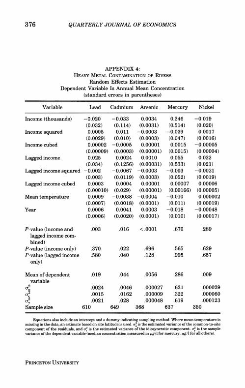
Finally, we turn to the heavy metals. A statistically significant relationship exists between concentrations of pollution and current and lagged GDP only for lead, cadmium, and arsenic.1" For lead, the relationship is mostly downward sloping; for cadmium it is flat, with perhaps a slight downturn at high levels of income; for arsenic it resembles an inverted U. The peak concentration of arsenic is estimated to occur at a per capita GDP of $4900, with a standard error of $250. The estimated slope of the curve is negative for lead and arsenic at both $10,000 and $12,000, and is statistically significant in each case.
To summarize, we find little evidence that environmental quality deteriorates steadily with economic growth. Rather, we find for most indicators that economic growth brings an initial phase of deterioration followed by a subsequent phase of improvement. We suspect that the eventual improvement reflects, in part, an in- creased demand for (and supply of) environmental protection at higher levels of national income. The turning points for the different pollutants vary, but in most cases they occur before a country reaches a per capita income of $8000. For seven of the fourteen indicators we find a statistically significant positive relationship between environmental quality and income for a middle-income country with a per capita GDP of $10,000. Only in one case (total coliform) do we find a significant adverse relation- ship at this income level.
Let us comment briefly on some of the other covariates included in our models. For the most part these variables have plausible effects. For example, dissolved oxygen is negatively associated with mean water temperature, whereas BOD, COD, and
11. Note that the number of observations in our samples for the heavy metals is much smaller than for most of the other pollutants.
370 QUARTERLY JOURNAL OF ECONOMICS
the coliforms are all positively associated with temperature, as the physical properties of water would lead one to expect. Air pollution is less severe in coastal cities (all else being equal), perhaps reflecting the dispersal caused by offshore winds or a smaller average inflow of pollution from neighboring cities. On the other hand, heavy particles are found in higher concentrations in cities located near a desert, while smoke is especially prevalent in densely populated areas.
Of particular interest are the estimated coefficients on the time variable. These coefficients indicate the extent to which environmental problems have been worsening or abating with time, apart from the effects of an expanding world economy. The state of the environment may deteriorate with time if concentra- tions of pollutants accumulate or if consumer tastes shift toward pollution-intensive goods. The opposite may occur if technological innovation makes abatement less costly or if increasing awareness causes an autonomous shift in public demands for environmental safeguards. We find that, at least as regards sulfur dioxide and smoke, urban air quality has tended to improve over time, once the effects of income have been controlled for. However, the opposite is true for most measures of river contamination.
V. CONCLUSIONS
We have examined the reduced-form relationship between national GDP and various indicators of local environmental condi- tions using panel data from the GEMS. Our indicator variables relate to urban air pollution and contamination in river basins. While admittedly these measures cover relatively few dimensions of environmental quality, our study is the most comprehensive possible given the limited availability of comparable data from different countries.
Contrary to the alarmist cries of some environmental groups, we find no evidence that economic growth does unavoidable harm to the natural habitat. Instead we find that while increases in GDP may be associated with worsening environmental conditions in very poor countries, air and water quality appear to benefit from economic growth once some critical level of income has been reached. The turning points in these inverted U-shaped relation- ships vary for the different pollutants, but in almost every case they occur at an income of less than $8000 (1985 dollars). For a
ECONOMIC GROWTH AND THE ENVIRONMENT 371
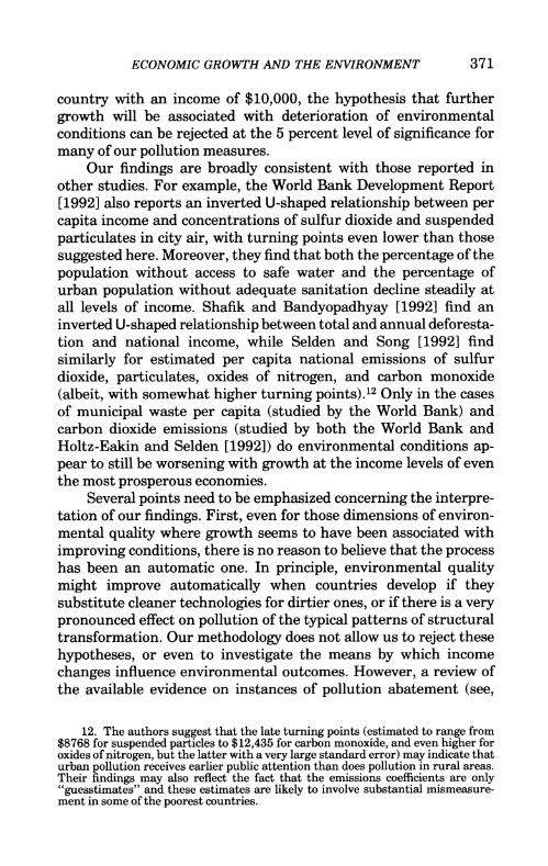
country with an income of $10,000, the hypothesis that further growth will be associated with deterioration of environmental conditions can be rejected at the 5 percent level of significance for many of our pollution measures.
Our findings are broadly consistent with those reported in other studies. For example, the World Bank Development Report [1992] also reports an inverted U-shaped relationship between per capita income and concentrations of sulfur dioxide and suspended particulates in city air, with turning points even lower than those suggested here. Moreover, they find that both the percentage of the population without access to safe water and the percentage of urban population without adequate sanitation decline steadily at all levels of income. Shafik and Bandyopadhyay [1992] find an inverted U-shaped relationship between total and annual deforesta- tion and national income, while Selden and Song [1992] find similarly for estimated per capita national emissions of sulfur dioxide, particulates, oxides of nitrogen, and carbon monoxide (albeit, with somewhat higher turning points).12 Only in the cases of municipal waste per capita (studied by the World Bank) and carbon dioxide emissions (studied by both the World Bank and Holtz-Eakin and Selden [1992]) do environmental conditions ap- pear to still be worsening with growth at the income levels of even the most prosperous economies.
Several points need to be emphasized concerning the interpre- tation of our findings. First, even for those dimensions of environ- mental quality where growth seems to have been associated with improving conditions, there is no reason to believe that the process has been an automatic one. In principle, environmental quality might improve automatically when countries develop if they substitute cleaner technologies for dirtier ones, or if there is a very pronounced effect on pollution of the typical patterns of structural transformation. Our methodology does not allow us to reject these hypotheses, or even to investigate the means by which income changes influence environmental outcomes. However, a review of the available evidence on instances of pollution abatement (see,
12. The authors suggest that the late turning points (estimated to range from $8768 for suspended particles to $12,435 for carbon monoxide, and even higher for oxides of nitrogen, but the latter with a very large standard error) may indicate that urban pollution receives earlier public attention than does pollution in rural areas. Their findings may also reflect the fact that the emissions coefficients are only "guesstimates" and these estimates are likely to involve substantial mismeasure- ment in some of the poorest countries.

372 QUARTERLY JOURNAL OF ECONOMICS
e.g., OECD [1991]) suggests that the strongest link between income and pollution in fact is via an induced policy response. As nations or regions experience greater prosperity, their citizens demand that more attention be paid to the noneconomic aspects of their living conditions. The richer countries, which tend to have relatively cleaner urban air and relatively cleaner river basins, also have relatively more stringent environmental standards and stricter enforcement of their environmental laws than the middle-income and poorer countries, many of which still have pressing environmen- tal problems to address.
Second, it is possible that downward sloping and inverted U-shaped patterns might arise because, as countries develop, they cease to produce certain pollution-intensive goods, and begin instead to import these products from other countries with less restrictive environmental protection laws. If this is the main explanation for the (eventual) inverse relationship between a country's income and pollution, then future development patterns could not mimic those of the past. Developing countries will not always be able to find still poorer countries to serve as havens for the production of pollution-intensive goods. However, the available evidence does not support the hypothesis that cross-country differ- ences in environmental standards are an important determinant of the global pattern of international trade (see, e.g., Tobey [1990] and Grossman and Krueger [1993]). While- some "environmental dumping" undoubtedly takes place, the volume of such trade is probably too small to account for the reduced pollution that has been observed to accompany episodes of economic growth.
Finally, it should be stressed that there is nothing at all inevitable about the relationships that have been observed in the past. These patterns reflected the technological, political, and economic conditions that existed at the time. The low-income countries of today have a unique opportunity to learn from this history and thereby avoid some of the mistakes of earlier growth experiences. With the increased awareness of environmental haz- ards and the development in recent years of new technologies that are cleaner than ever before, we might hope to see the low-income countries turn their attention to preservation of the environment at earlier stages of development than has previously been the case.
ECONOMIC GROWTH AND THE ENVIRONMENT 373
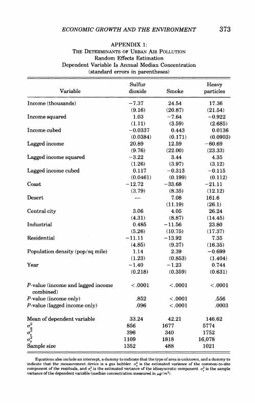
APPENDIX 1: THE DETERMINANTS OF URBAN AIR POLLUTION
Random Effects Estimation Dependent Variable Is Annual Median Concentration
(standard errors in parentheses)
Sulfur Heavy Variable dioxide Smoke particles
Income (thousands) -7.37 24.54 17.36 (9.16) (20.87) (21.54)
Income squared 1.03 -7.64 -0.922 (1.11) (3.59) (2.685)
Income cubed -0.0337 0.443 0.0136 (0.0384) (0.171) (0.0903)
Lagged income 20.89 12.59 -60.69 (9.76) (22.00) (23.33)
Lagged income squared -3.22 3.44 4.35 (1.26) (3.97) (3.12)
Lagged income cubed 0.117 -0.313 -0.115 (0.0461) (0.199) (0.112)
Coast -12.72 -33.68 -21.11 (3.79) (8.35) (12.12)
Desert - 7.08 161.6 (11.19) (26.1)
Central city 3.06 4.05 26.24 (4.31) (8.87) (14.45)
Industrial 0.485 -11.56 23.80 (5.26) (10.75) (17.37)
Residential -11.11 -13.92 7.35 (4.85) (9.37) (16.35)
Population density (pop/sq mile) 1.14 2.39 -0.699 (1.23) (0.853) (1.404)
Year -1.40 -1.23 0.744 (0.218) (0.359) (0.631)
P-value (income and lagged income <.0001 <.0001 <.0001 combined)
P-value (income only) .852 <.0001 .556 P-value (lagged income only) .096 <.0001 .0003
Mean of dependent variable 33.24 42.21 146.62 c02 856 1677 5774
2 396 340 1752 2 1109 1818 16,078
Sample size 1352 488 1021
Equations also include an intercept, a dummy to indicate that the type of area is unknown, and a dummy to indicate that the measurement device is a gas bubbler. 2 is the estimated variance of the common-to-site component of the residuals, and re2 is the estimated variance of the idiosyncratic component. '2 is the sample variance of the dependent variable (median concentration measured in pIg/m3).
374 QUARTERLY JOURNAL OF ECONOMICS
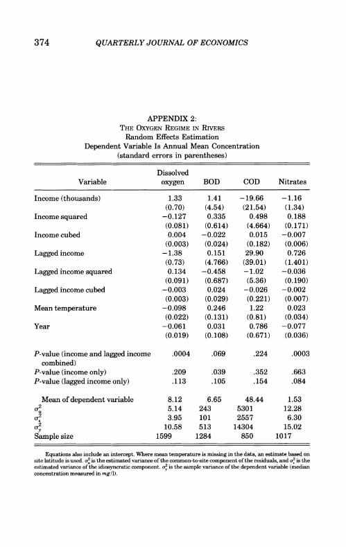
APPENDIX 2: THE OXYGEN REGIME IN RIVERs
Random Effects Estimation Dependent Variable Is Annual Mean Concentration
(standard errors in parentheses)
Dissolved Variable oxygen BOD COD Nitrates
Income (thousands) 1.33 1.41 -19.66 -1.16 (0.70) (4.54) (21.54) (1.34)
Income squared -0.127 0.335 0.498 0.188 (0.081) (0.614) (4.664) (0.171)
Income cubed 0.004 -0.022 0.015 -0.007 (0.003) (0.024) (0.182) (0.006)
Lagged income -1.38 0.151 29.90 0.726 (0.73) (4.766) (39.01) (1.401)
Lagged income squared 0.134 -0.458 -1.02 -0.036 (0.091) (0.687) (5.36) (0.190)
Lagged income cubed -0.003 0.024 -0.026 -0.002 (0.003) (0.029) (0.221) (0.007)
Mean temperature -0.098 0.246 1.22 0.023 (0.022) (0.131) (0.81) (0.034)
Year -0.061 0.031 0.786 -0.077 (0.019) (0.108) (0.671) (0.036)
P-value (income and lagged income .0004 .069 .224 .0003 combined)
P-value (income only) .209 .039 .352 .663 P-value (lagged income only) .113 .105 .154 .084
Mean of dependent variable 8.12 6.65 48.44 1.53 2 5.14 243 5301 12.28 2 3.95 101 2557 6.30 g2 10.58 513 14304 15.02
Sample size 1599 1284 850 1017
Equations also include an intercept. Where mean temperature is missing in the data, an estimate based on site latitude is used. a. is the estimated variance of the common-to-site component of the residuals, and od is the estimated variance of the idiosyncratic component. a' is the sample variance of the dependent variable (median concentration measured in mg/l).
ECONOMIC GROWTH AND THE ENVIRONMENT 375
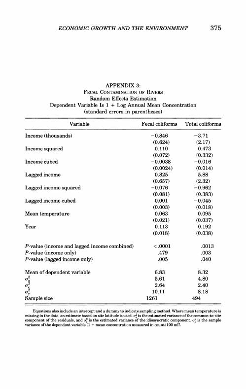
APPENDIX 3: FECAL CONTAMINATION OF RIVERS
Random Effects Estimation Dependent Variable Is 1 + Log Annual Mean Concentration
(standard errors in parentheses)
Variable Fecal coliforms Total coliforms
Income (thousands) -0.846 -3.71 (0.624) (2.17)
Income squared 0.110 0.473 (0.072) (0.332)
Income cubed -0.0038 -0.016 (0.0024) (0.014)
Lagged income 0.825 5.88 (0.657) (2.32)
Lagged income squared -0.076 -0.962 (0.081) (0.383)
Lagged income cubed 0.001 -0.045 (0.003) (0.018)
Mean temperature 0.063 0.095 (0.021) (0.037)
Year 0.113 0.192 (0.018) (0.038)
P-value (income and lagged income combined) <.0001 .0013 P-value (income only) .479 .003 P-value (lagged income only) .005 .040
Mean of dependent variable 6.83 8.32 2 5.61 4.80
oe2 2.64 2.40 o2 10.11 8.18 Sample size 1261 494
Equations also include an intercept and a dummy to indicate sampling method. Where mean temperature is missing in the data, an estimate based on site latitude is used. a, is the estimated variance of the common-to-site component of the residuals, and a,, is the estimated variance of the idiosyncratic component. a, is the sample variance of the dependent variable (1 + mean concentration measured in count/ 100 mUl.
376 QUARTERLY JOURNAL OF ECONOMICS
APPENDIX 4: HEAVY METAL CONTAMINATION OF RIVERS
Random Effects Estimation Dependent Variable Is Annual Mean Concentration
(standard errors in parentheses)
Variable Lead Cadmium Arsenic Mercury Nickel
Income (thousands) -0.020 -0.033 0.0034 0.246 -0.019 (0.032) (0.114) (0.0031) (0.514) (0.020)
Income squared 0.0005 0.011 -0.0003 -0.039 0.0017 (0.0029) (0.010) (0.0003) (0.047) (0.0016)
Income cubed 0.00002 -0.0005 0.00001 0.0015 -0.00005 (0.00009) (0.0003) (0.00001) (0.0015) (0.00004)
Lagged income 0.025 0.0024 0.0010 0.055 0.022 (0.034) (0.1256) (0.00031) (0.533) (0.021)
Lagged income squared - 0.002 -0.0067 -0.0003 -0.003 -0.0021 (0.003) (0.0119) (0.0003) (0.052) (0.0019)
Lagged income cubed 0.0003 0.0004 0.00001 0.00007 0.00006 (0.00010) (0.029) (0.00001) (0.00166) (0.00005)
Mean temperature 0.0009 -0.0038 -0.0004 -0.010 0.000002 (0.0007) (0.0018) (0.0001) (0.011) (0.00019)
Year 0.0006 0.0041 0.0003 -0.018 -0.00048 (0.0006) (0.0020) (0.0001) (0.010) (0.00017)
P-value (income and .003 .016 <.0001 .670 .289 lagged income com- bined)
P-value (income only) .370 .022 .696 .565 .629 P-value (lagged income .580 .040 .128 .995 .657
only)
Mean of dependent .019 .044 .0056 .286 .009 variable
2 .0024 .0046 .000027 .631 .000029
a2 .0015 .0162 .000009 .322 .000060 y2 .0021 .028 .000048 .619 .000123
Sample size 610 649 368 637 350
Equations also include an intercept and a dummy indicating sampling method. Where mean temperature is missing in the data, an estimate based on site latitude is used. o2 is the estimated variance of the common-to-site component of the residuals, and o,2 is the estimated variance of the idiosyncratic component. a, is the sample variance of the dependent variable (median concentration measured in Ag/l for mercury, Ag/l for all others).
PRINCETON UNIVERSITY
ECONOMIC GROWTH AND THE ENVIRONMENT 377
REFERENCES
Bennett, Burton G., Jan G. Kretzschmar, Gerald G. Akland, and Henk W. de Koning, "Urban Air Pollution Worldwide," Environmental Science and Tech- nology, XIX (1985), 298-304.
Dockery, Douglas W., et al., "An Association Between Air Pollution and Mortality in Six U. S. Cities," New England Journal of Medicine, CCCXXIX (1993), 1753-59.
Grossman, Gene M, and Alan B. Krueger, "Environmental Impacts of a North American Free Trade Agreement," in The U. S.-Mexico Free Trade Agreement, P. Garber, ed. (Cambridge, MA: MIT Press, 1993).
Holtz-Eakin, Douglas, and Thomas M. Selden, "Stoking the Fires? CO2 Emissions and Economic Growth," NBER Working Paper No. 4248, 1992.
Kormondy, Edward J., ed., International Handbook of Pollution Control (New York and Westport, CT: Greenwood Press, 1989).
Lave, Lester B., and E. P. Seskin, "Air Pollution and Human Health," Science, CLXIX (1970), 723-33.
Organization for Economic Cooperation and Development, The State of the Environment (Paris: OECD, 1991).
Selden, Thomas M., and Daqing Song, "Environmental Quality and Development: Is There a Kuznets Curve for Air Pollution Emissions?" Journal of Environmen- tal Economics and Management, XXVII (1994), 147-62.
Shafik, Nemat, and Sushenjit Bandyopadhyay, "Economic Growth and Environmen- tal Quality: Time Series and Cross-Country Evidence," World Bank Policy Research Working Paper WPS 904, 1992.
Summers, Robert, and Alan Heston, "The Penn World Table (Mark 5): An Expanded Set of International Comparisons, 1950-1988," Quarterly Journal of Economics, CVI (1989), 327-69.
Syrquin, Moshe, "Patterns of Structural Change," in Handbook of Development Economics, vol. 1, H. Chenery and T. N. Srinivasan, eds. (Amsterdam: North-Holland, 1989).
Tobey, James A., "The Effects of Domestic Environmental Policies on Patterns of World Trade: An Empirical Test," Kyklos, XLIII (1990), 191-209.
U. S. Environmental Protection Agency, Air Quality Criteria for Particulate Matter and Sulfur Oxides (Research Triangle Park, NC: U. S. Environmental Protec- tion Agency, 1982).
World Bank, World Development Report 1992: Development and the Environment (Washington, DC: The World Bank, 1992).
World Resources Institute, World Resources 1988-89 (New York: Oxford Univer- sity Press, 1988).


![1. Introduction - NBER · 2020. 3. 20. · scale, technique and composition effects has proven useful in other contexts [see Grossman and Krueger (1993), Copeland and Taylor (1994,1995)]](https://img.pdfslide.us/doc/110x75/611bd9537a48324096699165/1-introduction-nber-2020-3-20-scale-technique-and-composition-effects-has.jpg)