Authors: 1,2, Stephen L. Macknik1,3, Susana Martinez …smc.neuralcorrelate.com/files/publications/mccamy_jphysiology2014.pdf · This is an Accepted Article that has been peer-reviewed

This is an Accepted Article that has been peer-reviewed and approved for publication in the The Journal of

Physiology, but has yet to undergo copy-editing and proof correction. Please cite this article as an 'Accepted

Article'; doi: 10.1113/jphysiol.2014.279059.

This article is protected by copyright. All rights reserved. 0

Title: Different fixational eye movements mediate the prevention and the reversal of visual

fading

Running title: Fading prevention by fixational eye movements

Authors: Michael B. McCamy1,2

, Stephen L. Macknik1,3

, Susana Martinez-Conde1

Affiliations: 1Department of Neurobiology, Barrow Neurological Institute, Phoenix, AZ,

USA

2School of Mathematical and Statistical Sciences, Arizona State University, Tempe, AZ,

USA

3Department of Neurosurgery, Barrow Neurological Institute, Phoenix, AZ, USA

Keywords: Vision, adaptation, eye position

Total number of words (excluding references and figure legends): 7419

Table of Contents: Neuroscience - behavioural/systems/cognitive

Corresponding author: Correspondence should be addressed to Susana Martinez-Conde,

Department of Neurobiology, Barrow Neurological Institute, 350 W Thomas Rd. Phoenix,

AZ 85013, USA. E-mail: [email protected]

Key points summary:

Fixational eye movements (microsaccades, drift, and tremor) are thought to improve

visibility during fixation by thwarting neural adaptation to unchanging stimuli, but

how the different fixational eye movements influence this process is a matter of

debate.

Prior studies confounded the reversal of fading (where vision is restored after fading)

with its prevention (where fading is blocked before it happens). We found that,

whereas microsaccades are most important to reversing fading, both microsaccades

and drift help to prevent it.

mailto:[email protected]


Drift’s contribution to preventing fading is potentially larger than that of

microsaccades, but microsaccades prevent fading with higher efficacy than drift.

Microsaccades prevent foveal and peripheral fading in an equivalent fashion, and

microsaccadic efficacy does not depend on microsaccade size, number, or direction.

Further, faster drift may prevent fading better than slower drift

These combined findings help reconcile the long-standing controversy concerning the

roles of microsaccades and drift in visibility during fixation

ABSTRACT

Fixational eye movements (FEMs; including microsaccades, drift and tremor) are thought to

improve visibility during fixation by thwarting neural adaptation to unchanging stimuli, but

how the different FEM types influence this process is a matter of debate. Attempts to answer

this question have been hampered by the failure to distinguish between the prevention of

fading (where fading is blocked before it happens in the first place) and the reversal of fading

(where vision is restored after fading has already occurred). Because fading during fixation is

a detriment to clear vision, the prevention of fading --which avoids visual degradation before

it happens-- is a more desirable scenario than improving visibility after fading has occurred.

Yet, previous studies have not examined the role of FEMs in the prevention of fading, but

have focused on visual restoration instead. Here we set out to determine the differential

contributions and efficacies of microsaccades and drift to preventing fading in human vision.

Our results indicate that both microsaccades and drift mediate the prevention of visual fading.

We also found that drift is a potentially larger contributor to preventing fading than

microsaccades, although microsaccades are more effective than drift. Microsaccades

moreover prevented foveal and peripheral fading in an equivalent fashion, and their efficacy

was independent of their size, number, and direction. Our data also suggest that faster drift

may prevent fading better than slower drift. These findings may help to reconcile the long-

standing controversy concerning the comparative roles of microsaccades and drift in visibility

during fixation.


INTRODUCTION

When eye movements are eliminated, stationary or unchanging objects fade from

perception (Ditchburn and Ginsborg, 1952; Riggs and Ratliff, 1952 p.52; Yarbus, 1957).

Outside of the laboratory, our eyes are never still, however: even when we attempt to fixate

our gaze on an object of interest, small ocular motions, called fixational eye movements

(FEMs: including microsaccades, drift and tremor) shift our eye position. FEMs are thought

to help visibility during fixation by thwarting neural adaptation to unchanging stimuli

(Martinez-Conde et al., 2004, 2013; Engbert and Mergenthaler, 2006), but how the different

FEM types influence this process is a matter of debate. Attempts to answer this question have

been hampered by the failure to distinguish between the prevention of fading (where fading is

blocked before it happens in the first place) and the reversal of fading (where vision is

restored after fading has already occurred). There has been a relative dearth of research to

specify the oculomotor mechanisms underlying the prevention of fading.

Because fading during fixation is a detriment to clear vision, the prevention of fading

--which avoids visual degradation before it happens during fading-- is a more desirable

scenario than improving visibility after fading has occurred. Thus, determining how the

different eye movement types prevent fading is more important than establishing how they

restore visibility once fading has taken place. Yet, previous studies have not examined the

role of FEMs in the prevention of fading , but have focused on restoration instead (Martinez-

Conde et al., 2006; Troncoso et al., 2008; McCamy et al., 2012; Costela et al., 2013). It

follows that no research to date has determined the differential effects of each individual

FEM type on fading prevention, as we now do here. Recently, we developed a principled

quantitative method to determine the contribution and efficacy of microsaccades and other

eye movements to reversing fading during fixation (McCamy et al., 2012). Here we have

enhanced the method to determine the differential contributions and efficacies of

microsaccades and drift to preventing fading.

Our results indicate that both microsaccades and drift work to prevent fading. We also

found that drift is a potentially larger contributor to fading prevention than microsaccades,

although microsaccades are more effective than drift. Microsaccades moreover prevented

foveal and peripheral fading in an equivalent fashion, and their efficacy was independent of

their size, number, and direction. Our data also suggest that faster drift may prevent fading

better than slower drift. These findings may help to reconcile the long-standing controversy

concerning the comparative roles of microsaccades and drift in visibility during fixation.


METHODS

Ethics statement

Experiments were approved by the Barrow Neurological Institute Institutional Review

Board (protocol number 04BN039) and conformed to the Declaration of Helsinki. Written

informed consent was obtained from each participant.

Subjects

Seven subjects (5 males) with normal or corrected-to-normal vision participated in the

experiments. Six subjects were naive and were paid $15/session. For one subject, 2

experimental sessions were discarded due to pupil occlusion (which made the data too noisy

for accurate microsaccade detection). Three other subjects lost 5 or less trials of data, out of

256 trials, due to pupil occlusion (the eye position was lost by the eye tracker); these data

losses did not significantly affect the results.

Experimental design

Subjects rested their forehead and chin on the EyeLink 1000 head/chin support ~57

cm away from a linearized video monitor (Barco Reference Calibrator V, 75 Hz refresh rate).

The experiment consisted of 5 ~ 1-1.5 hours sessions, each including 64 randomly

interleaved trials. The first session was counted as a training session and not included in the

analyses.

Illusory fading condition. While fixating a small red spot (with a diameter of 0.05

degrees of visual angle (deg)) on the center of the screen, subjects continuously reported

whether a stimulus was faded/fading (button press) or intensified/intensifying (button release)

(Martinez-Conde et al., 2006) (Fig. 1A). To start the trial, subjects pressed a key and the

stimulus appeared on the screen. The stimulus was a two-lobe Gabor patch with a peak-to-

trough width of 2.5 deg (Gaussian standard deviations of x = 1.5 deg and y = 1 deg; sine wave

period of 5 deg; sine wave phase of 0 deg). The Gabor had a maximum contrast of 40% from

peak-to-trough and the same average luminance (50%) as the background. The Gabor was

presented at random eccentricities of 0 deg, 3 deg, 6 deg, 9 deg (measured from the center of

the fixation point to the center of the Gabor). The position of the Gabor varied randomly

across trials at one of the eight points of the compass, to control for possible contrast

adaptation effects across trials. The orientation of the Gabor also varied randomly between 0º


(here, ° represents circular angle) and 360º in each trial, to control for orientation adaptation

effects. After 30 seconds, the stimuli disappeared and the trial ended. To disregard the

potential effect of the initial stimulus onset transient at the start of each trial, we conducted

analyses only on data recorded after the first second of the trial. A minimum average of 2

transitions per 30 second trial was imposed to ensure that the subjects experienced the

illusion; one subject was discontinued after the training session due to this restriction.

Real fading condition. Experimental details were as in the Illusory fading condition;

however, the Gabor now physically faded and intensified (Fig. 1B). The Gabor always started

at 40% contrast. Then, according to the times of transitions reported by the subject in prior

randomly chosen Illusory fading trials, the Gabor faded/intensified in step fashion to a

lower/higher contrast randomly chosen from the set: 0%, 10%, 20%, 30%, 40%. To avoid

perceptual transitions due to illusory fading which might interfere with the physical

transitions, the Gabor moved at a constant speed (0.1 cycles/s) in a circular path of 1.25 deg

radius. The parameters for the movement of the Gabor were the minimal values found to

make the Gabor continuously visible at any given contrast.

Subjects performed this task well (95 ± 15% of real fadings detected; 97 ± 16% of

reports of real fading were hits), and their reaction times provided tight estimates of reaction

times in the Illusory fading condition, necessary for the contribution and efficacy analyses

(Fig. 3). The data from the Real fading trials were not otherwise subjected to additional

analyses.

<<<PLEASE INSERT FIGURE 1 AROUND HERE>>>

Eye movement analyses

Microsaccade and blink detection. Eye position was acquired noninvasively with a

fast video-based eye tracker at 500 Hz (EyeLink 1000, SR Research). EyeLink 1000 records

eye movements simultaneously in both eyes (instrument noise 0.01 deg RMS). We identified

and removed blink periods as portions of the raw data where pupil information was missing.

We also removed portions of data where very fast decreases and increases in pupil area

occurred (> 50 units/sample, such periods are probably semi-blinks where the pupil is never

fully occluded) (Troncoso et al., 2008). We added 200 ms before and after each blink/semi-

blink to eliminate the initial and final parts where the pupil was still partially occluded

(Troncoso et al., 2008). Saccades were identified with a modified version of the algorithm


developed by Engbert & Kliegl (Engbert and Kliegl, 2003; Laubrock et al., 2005; Engbert,

2006; Engbert and Mergenthaler, 2006; Rolfs et al., 2006) with = 4 (used to obtain the

velocity threshold) and a minimum saccadic duration of 6 ms. To reduce the amount of

potential noise, we considered only binocular saccades, that is, saccades with a minimum

overlap of one data sample in both eyes (Laubrock et al., 2005; Engbert, 2006; Engbert and

Mergenthaler, 2006; Rolfs et al., 2006).

Some saccades are followed by a fast and small saccadic eye movement in the

opposite direction, called dynamic overshoot, which is often more prominent in the eye that

moves in the abducting direction (Kapoula et al., 1986). Unlike the return saccade in a

square-wave jerk, a dynamic overshoot follows a saccade with very short latency between the

two movements. We identified dynamic overshoots as saccades that occurred less than 20 ms

after a preceding saccade (Møller et al., 2002) and we did not regard them as new saccades.

Instead, we added the duration of the overshoot into the duration of the saccade, thus

considering it part of the saccade. Microsaccades were defined as saccades with magnitude <

1 deg in each eye (Martinez-Conde et al., 2004). To calculate (micro)saccade properties such

as magnitude and peak velocity we averaged the values for the right and left eyes. The mean

of the median intersaccadic interval (including saccades and microsaccades) across subjects

was 285 ms (± 27 s.e.m.).

Drift periods. Drift periods were defined as the eye-position epochs between

(micro)saccades and blinks. We removed 10 ms from the start and end of each of these

epochs (because of imperfect detection of blinks and (micro)saccades), and we filtered the

remaining eye-position data with a low-pass Butterworth filter of order 13 and a cut-off

frequency of 30 Hz (Di Stasi et al., 2013). Because drifts are not generally conjugate

(Krauskopf et al., 1960; Yarbus, 1967; Martinez-Conde et al., 2004), we used data from both

the left and right eye. For instance, any given drift period had a unique maximum (mean,

standard deviation) drift speed for each eye. The values reported in Figs. 6-7 were found by

averaging all data from both eyes. The average duration of drifts across subjects was 1.11 s (±

0.19 s.e.m.). The mean maximum drift duration across subjects was 11.24 s (± 1.40 s.e.m.).

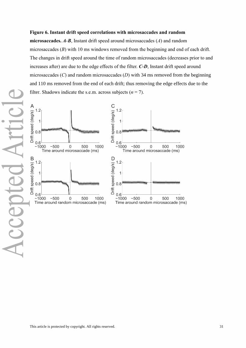
Removing filter edge effects. Before calculating drift properties (such as the mean and

maximum speed), we removed an additional 34 ms from the beginning and 110 ms from the

end of each drift period as defined above, to reduce edge effects due to the filter. We

determined that filter edge effects caused artificial increases/decreases in drift speed before


microsaccades (Fig. 6A) because we observed increases/decreases seen in the drift speed

correlation with random microsaccades (Fig. 6B). The values (34 and 110 ms) chosen were

determined by finding when the drift speed around random microsaccades (black solid line in

Fig. 6B) was first within 5% of the average drift speed (dotted horizontal line Fig. 6B). This

choice resulted in a flat correlation of drift speed with random microsaccades; thus it

removed any detectable edge effects (Fig. 6D). The removal of the edge effects due to the

filter was especially important in our analyses because microsaccade rates differ between the

two regions compared in Fig. 7. If filter edge effects had remained, we would have obtained

artificial results because the increased numbers of microsaccades would have resulted in

more instances of higher drift speeds. Finally, because we had to remove 144 ms from each

drift’s duration (34 ms from the beginning and 110 ms from the end), drifts shorter than 300

ms were not analyzed in Fig. 7A.

Removing post-saccadic drift effects. After we removed the edge effects due to the

filter, we still observed increases in drift speed after microsaccades (Fig. 6C). These are real

increases as opposed to artificial ones caused by the filter because these increases are not

seen for the correlation with random microsaccades (Fig. 6D). This agrees with recent

research reporting increased post-saccadic drift (Chen and Hafed, 2013). To analyze drift

properties without the effects of post-saccadic drift (Fig. 7B), we removed 380 ms from the

beginning of each drift (and still the 110 ms from the end for the filter edge effects) before

calculating drift properties. This value was determined by finding where the drift speed after

a microsaccade (black solid line in Fig. 6C) first equaled the average drift speed (dotted

horizontal line Fig. 6C). The correlation of drift speed with microsaccades becomes

completely flat with this choice (Fig. 6A). Finally, because we had to remove 490 ms from

each drift’s duration (380 ms from the beginning for post-saccadic drift and 110 ms from the

end for the filter edge effects), drifts shorter than 600 ms were not analyzed in Fig. 7B.


Contribution and efficacy

Correlograms and notation. Let ,MX ,SX ,BX and FX denote the microsaccade,

saccade, blink, and fading report (F) stochastic onset processes, and A M S BX X X X of

all eye movements. Let *N be the number of times * occurs. Let ( )

( ) ( ) ( )AF F

j t

A

I

t j t jX X


(where ( )I t is as above), be the correlation of AX with FX , and ( 1) 1

( ) ξ ( )t w n

AF AFt wnn t

the correlogram of AX with FX (bin width w = 50 ms). We take the convention that ( )AF n

refers to the bin value of AF at bin n, and ( )AF t refers to the bin value of bin n, where wn

t w(n + 1) 1 (we adopt the same convention for any other function that is binned in time,

such as ,AFB defined below).

Contribution and efficacy development. The concepts of contribution and efficacy

have been used to measure the strength of connection between two neurons (Levick et al.,

1972; Mastronarde, 1987; Aertsen et al., 1989; Reid and Alonso, 1995; Alonso et al., 1996,

2001; Usrey et al., 1998, 1999), and recently in determining the impact of microsaccades in

restoring faded vision (McCamy et al., 2012). Here we are concerned with the impact of

microsaccades in the prevention of fading. Thus, we include no analyses concerning the

efficacy and contribution of different eye movement types to the reversal of fading

(previously reported by (McCamy et al., 2012), using this dataset). The present analyses do

not overlap with the previous analyses unless otherwise noted.

We defined the contribution of microsaccades to the prevention of fading, ( ),R M as

the percentage of fading prevention reports (R; to be defined below) caused by

microsaccades, and the efficacy of microsaccades in preventing fading, ( ),R M as the

percentage of microsaccades which caused a prevented fading report. That is:

number of s caused by microsaccades, and

total number of s( )R

R

RM

number of microsaccades which caused a .

number of microsaccades eligible to cause( )

a R M

R

R

To calculate the contribution and efficacy of microsaccades in preventing fading,

along with those of other eye movements, we estimated the number of Rs caused by

microsaccades, as well as those caused by saccades, blinks, and combinations thereof.

Because we did not ask subjects (nor could we have asked them) to report when the stimulus

was prevented from fading, we first had to take some steps to define what a report of fading

prevention was. The most crucial step to this was to find the microsaccades (and other eye

movements) that we know did not prevent fading (i.e. did not prevent an F). Importantly,

only eye movements occurring during a specific window of time in the “intensified region”

(i.e. the time in which the stimulus was reported as intensified/intensifying) did not prevent


an F. We call this window of time the “trough interval” because it corresponds to the trough

of the correlogram between eye movements and Fs, and we denote it by .

Defining the trough interval . We estimated in two steps: 1) First, we used the

distribution of the subjects’ reaction times to target fading in the Real fading condition

(which we denote by Frt) to estimate the reaction times in the Illusory fading condition. We

required to be contained within the interval [ , ]F b a (where the interval [a, b] contains

98% of the data from Frt, discarding the top and bottom 1%; Fig. 3A); we restricted to be

contained in F because eye movements in F are the only ones which did not prevent an F,

as these are the only eye movements which occurred within the reaction times of the subject.

2) We further refined 's limits as follows. Let AF be the correlogram of all eye movement

onsets (microsaccades, saccades, and blinks) with Fs. Also, let the baseline, ,AFB be the

expected value of AF assuming that the eye movements and Fs were independent

(Mastronarde, 1987; McCamy et al., 2012) (see the "Correlogram baseline and trough

interval" section below for an exact definition of the baseline; Fig. 3B). We took as the

interval of time inside of F where AF was below AFB (Levick et al., 1972; Mastronarde,

1987; Palm et al., 1988; Aertsen et al., 1989; Alonso et al., 1996; Usrey et al., 1998, 1999;

Grun, 2009; McCamy et al., 2012) and contiguous with the minimum bin closest to the Fs

(see the "Correlogram baseline and trough interval" section below for an exact definition of ;

Fig. 3B). If no bin of AF within F was significantly below AFB , we took as nonexistent

and the contribution and efficacy as zero for that subject.

Defining prevented fading reports. Having defined , we defined a report of the

prevention of fading (R) as follows. If for a given interval of time [x, y], whose duration

equals 's duration, and which is contained in the intensified region, the stimulus was not

subsequently reported as fading at some point during the interval [y, y + a], we equated that

to a subjects report, at time t = y + a, that the stimulus was prevented from fading. This

means that any given interval with 's duration inside of the intensified region occurring

before satisfies this criterion. Any interval or any interval after does not satisfy this

criterion by definition. We call the intensified region before the prevention region and

denote it by (Fig. 3B). To obtain distinct reports of fading prevention with corresponding

distinct prevention intervals, we divided the prevention region into disjoint "prevention

intervals," which we denote by ,i of the same duration as . See “Prevention and eligible


intervals” section for more details. Each i corresponds to exactly one report of fading

prevention (i.e. one R). Our goal was to estimate the number of microsaccades in the i that

caused an R.

Contribution and efficacy definitions To calculate the number of Rs caused by

microsaccades, one cannot simply add the number of microsaccades that occurred within the

,i for two reasons: 1) Some i may have contained multiple microsaccades or

combinations of microsaccades and other eye movements (i.e. blinks or saccades) (Fig. 4).

The simple addition of the number of microsaccades in all the i could thus result in some

Rs being counted as caused more than once, leading to an overestimate of microsaccadic

contribution and efficacy. 2) Some microsaccades that occurred within a i may not have

caused an R; thus, counting them as causal would overestimate their contribution and

efficacy.


Multiple eye movements To account for the possibility that multiple eye movements

may have led to an R (reason 1 above), we defined the event: M = event that only

microsaccades (one or more) occurred over a time interval of duration equal to 's duration

(Fig. 4). We defined analogous events for saccades (S), blinks (B), microsaccades and

saccades (MS), microsaccades and blinks (MB), saccades and blinks (SB), and

microsaccades, saccades, and blinks (MSB) and calculated the contribution, ( ),R E and

efficacy, ( ),R E of each event E = M, S, B, MS, MB, SB, and MSB. That is, for each E, we

calculated:

number of s caused by , and

total number of s( )R

R E

RE

number of which caused a .

number of eligible to cau(

s)

e a R

R

E RE

E

The definitions of the ocular events E ensure a one-to-one correspondence between the

caused Rs and the causal ocular events within the ;i thus, the numerators of ( )R E and

( )R E represent the same quantity even though their semantics differ.

Control level To account for the possibility that some of the Es occurring within the

i may not have caused a R (reason 2 above), we estimated the number of non-causal Es

within the i from the trough interval . Es in did not prevent fading, but they were


nevertheless eligible to prevent fading because they occurred in the intensified region. We

call the probability of an E occurring within the , ( | ),P E the control level. If RN was the

total number of Rs, then the expected number of non-causal Es that occurred within the i

was estimated, using the control level, as ( | ) .RP E N

Definitions The total number of Es that occurred is ( ) ,| i RP E N thus we took the

difference between ( | ) RiP E N and ( | ) RP E N as our estimate of the causal number of Es,

i.e. the numerator of both ( )R E and ( ).R E Therefore, the contribution and efficacy of an

ocular event E are:

( | ) ( | )( | ) ( | ), a d) n( R R

R

iR i

P E N PE

E NP E P E

N

( | ) ( | )

[ ( | ) ( | )]) ,( R R

E

i RiR

E

P E N P E N NP E P E

N NE

where EN is the number of Es that were eligible to cause an R (Fig. 5). Eligible Es are those

that occurred in the intensified region before the termination of (we call this the "eligible

region" and denote it by ); Es that occurred after cannot be counted as eligible because the

subject’s perception had already changed at some point during the interval and so those Es

were not in the intensified region and were thus unable to prevent fading. We took

( | ) ,EN P E T d where d is the duration of , ( | )P E was estimated using "eligible

intervals" in the same way ( | )iP E was found (see the "Prevention and eligible intervals"

section below; Fig. 3B), and T is the amount of time spent in by the subject.


Correlogram baseline and trough interval. We estimated the baseline, ,AFB using

the data from the intensified region before .F We chose this region because microsaccades

and other eye movements in this region are completely independent of the Fs as they

occurred outside of the reaction time window in both directions of time. If {0,1}J indexes

when AX is in the intensified region before ,F then we took the baseline rate to be

( ) ( ).

( )

AtA

t

X t J tr

J t


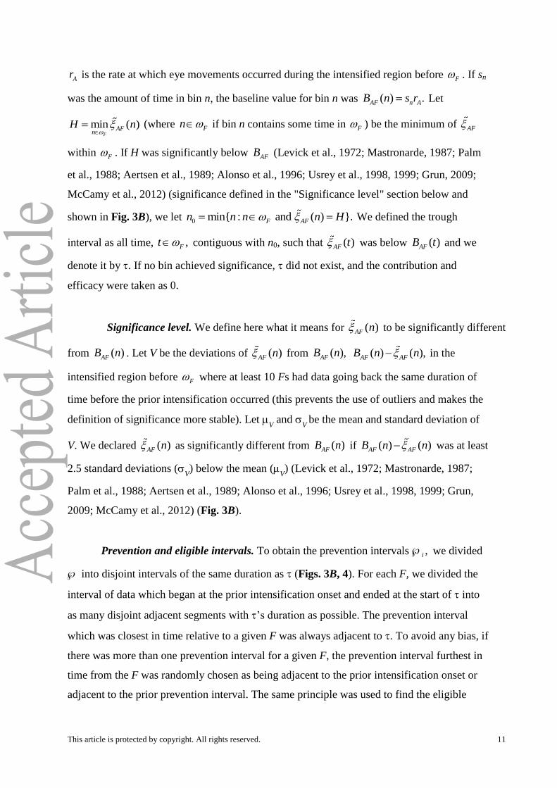
Ar is the rate at which eye movements occurred during the intensified region before F . If sn

was the amount of time in bin n, the baseline value for bin n was ( ) .AF n AB n s r Let

min ( )F

AFn

H n

(where Fn if bin n contains some time in F ) be the minimum of AF

within F . If H was significantly below AFB (Levick et al., 1972; Mastronarde, 1987; Palm

et al., 1988; Aertsen et al., 1989; Alonso et al., 1996; Usrey et al., 1998, 1999; Grun, 2009;

McCamy et al., 2012) (significance defined in the "Significance level" section below and

shown in Fig. 3B), we let 0 min{ : and ( ) }.F AFn n n n H We defined the trough

interval as all time, ,Ft contiguous with n0, such that ( )AF t was below ( )AFB t and we

denote it by . If no bin achieved significance, did not exist, and the contribution and

efficacy were taken as 0.

Significance level. We define here what it means for ( )AF n to be significantly different

from ( )AFB n . Let V be the deviations of ( )AF n from ( ),AFB n ( ) ( ),AF AFB n n in the

intensified region before F where at least 10 Fs had data going back the same duration of

time before the prior intensification occurred (this prevents the use of outliers and makes the

definition of significance more stable). Let V and

V be the mean and standard deviation of

V. We declared ( )AF n as significantly different from ( )AFB n if ( ) ( )AF AFn nB was at least

2.5 standard deviations (V) below the mean (

V) (Levick et al., 1972; Mastronarde, 1987;

Palm et al., 1988; Aertsen et al., 1989; Alonso et al., 1996; Usrey et al., 1998, 1999; Grun,

2009; McCamy et al., 2012) (Fig. 3B).

Prevention and eligible intervals. To obtain the prevention intervals ,i we divided

into disjoint intervals of the same duration as (Figs. 3B, 4). For each F, we divided the

interval of data which began at the prior intensification onset and ended at the start of into

as many disjoint adjacent segments with ’s duration as possible. The prevention interval

which was closest in time relative to a given F was always adjacent to . To avoid any bias, if

there was more than one prevention interval for a given F, the prevention interval furthest in

time from the F was randomly chosen as being adjacent to the prior intensification onset or

adjacent to the prior prevention interval. The same principle was used to find the eligible


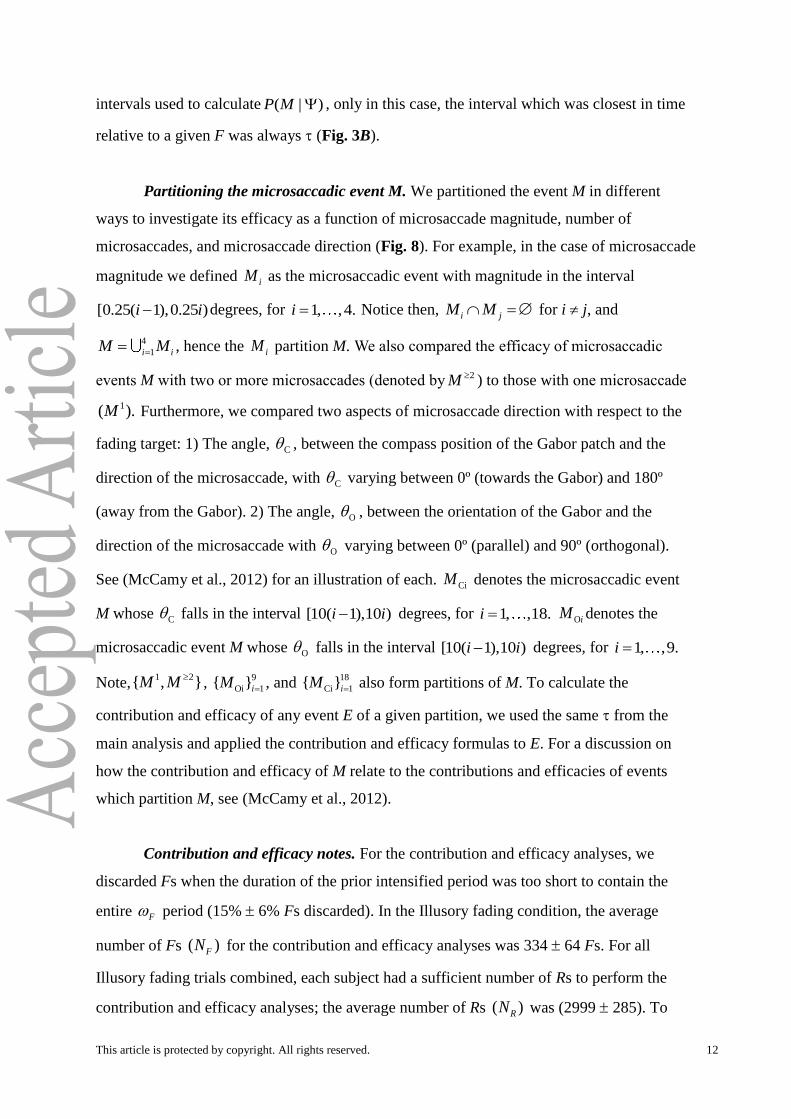
intervals used to calculate ( | )P M , only in this case, the interval which was closest in time

relative to a given F was always (Fig. 3B).

Partitioning the microsaccadic event M. We partitioned the event M in different

ways to investigate its efficacy as a function of microsaccade magnitude, number of

microsaccades, and microsaccade direction (Fig. 8). For example, in the case of microsaccade

magnitude we defined iM as the microsaccadic event with magnitude in the interval

[0.25( 1),0.25 )i i degrees, for 1, ,4.i Notice then, i jM M for i j, and

4

1i iM M , hence the iM partition M. We also compared the efficacy of microsaccadic

events M with two or more microsaccades (denoted by 2M ) to those with one microsaccade

1( ).M Furthermore, we compared two aspects of microsaccade direction with respect to the

fading target: 1) The angle, C , between the compass position of the Gabor patch and the

direction of the microsaccade, with C varying between 0º (towards the Gabor) and 180º

(away from the Gabor). 2) The angle, O , between the orientation of the Gabor and the

direction of the microsaccade with O varying between 0º (parallel) and 90º (orthogonal).

See (McCamy et al., 2012) for an illustration of each. CiM denotes the microsaccadic event

M whose C falls in the interval [10( 1),10 )i i degrees, for 1, ,18.i OiM denotes the

microsaccadic event M whose O falls in the interval [10( 1),10 )i i degrees, for 1, ,9.i

Note,1 2{ , }M M

, 9

Oi 1{ }iM , and 18

Ci 1{ }iM also form partitions of M. To calculate the

contribution and efficacy of any event E of a given partition, we used the same from the

main analysis and applied the contribution and efficacy formulas to E. For a discussion on

how the contribution and efficacy of M relate to the contributions and efficacies of events

which partition M, see (McCamy et al., 2012).

Contribution and efficacy notes. For the contribution and efficacy analyses, we

discarded Fs when the duration of the prior intensified period was too short to contain the

entire F period (15% 6% Fs discarded). In the Illusory fading condition, the average

number of Fs ( )FN for the contribution and efficacy analyses was 334 64 Fs. For all

Illusory fading trials combined, each subject had a sufficient number of Rs to perform the

contribution and efficacy analyses; the average number of Rs ( )RN was (2999 285). To


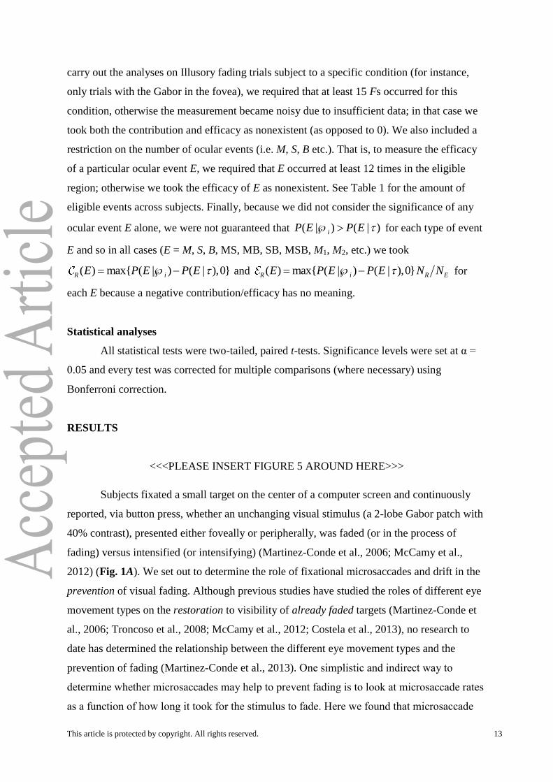
carry out the analyses on Illusory fading trials subject to a specific condition (for instance,

only trials with the Gabor in the fovea), we required that at least 15 Fs occurred for this

condition, otherwise the measurement became noisy due to insufficient data; in that case we

took both the contribution and efficacy as nonexistent (as opposed to 0). We also included a

restriction on the number of ocular events (i.e. M, S, B etc.). That is, to measure the efficacy

of a particular ocular event E, we required that E occurred at least 12 times in the eligible

region; otherwise we took the efficacy of E as nonexistent. See Table 1 for the amount of

eligible events across subjects. Finally, because we did not consider the significance of any

ocular event E alone, we were not guaranteed that ( | ) ( | )iP E P E for each type of event

E and so in all cases (E = M, S, B, MS, MB, SB, MSB, M1, M2, etc.) we took

( |( ) max{ ) ( | ),0}R iP E P EE and ( ) max{ ( | ) ( | ),0}iR R EPE E P E N N for

each E because a negative contribution/efficacy has no meaning.

Statistical analyses

All statistical tests were two-tailed, paired t-tests. Significance levels were set at α =

0.05 and every test was corrected for multiple comparisons (where necessary) using

Bonferroni correction.

RESULTS


Subjects fixated a small target on the center of a computer screen and continuously

reported, via button press, whether an unchanging visual stimulus (a 2-lobe Gabor patch with

40% contrast), presented either foveally or peripherally, was faded (or in the process of

fading) versus intensified (or intensifying) (Martinez-Conde et al., 2006; McCamy et al.,

2012) (Fig. 1A). We set out to determine the role of fixational microsaccades and drift in the

prevention of visual fading. Although previous studies have studied the roles of different eye

movement types on the restoration to visibility of already faded targets (Martinez-Conde et

al., 2006; Troncoso et al., 2008; McCamy et al., 2012; Costela et al., 2013), no research to

date has determined the relationship between the different eye movement types and the

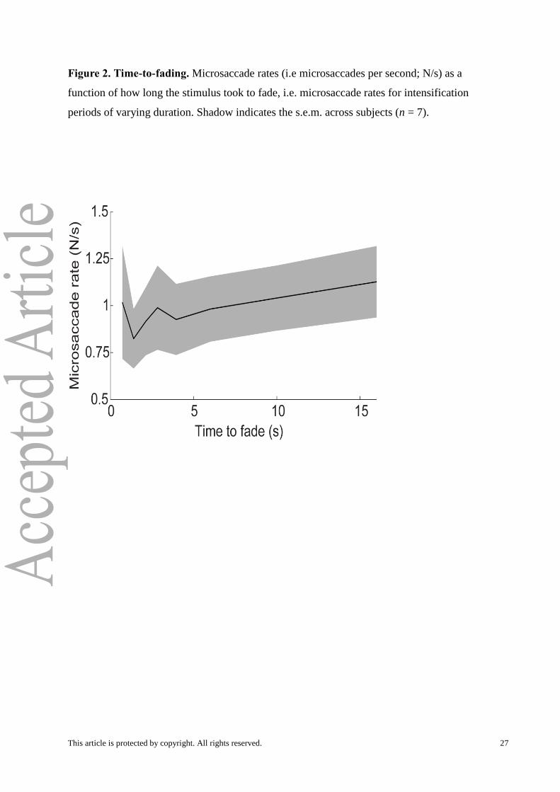
prevention of fading (Martinez-Conde et al., 2013). One simplistic and indirect way to

determine whether microsaccades may help to prevent fading is to look at microsaccade rates

as a function of how long it took for the stimulus to fade. Here we found that microsaccade


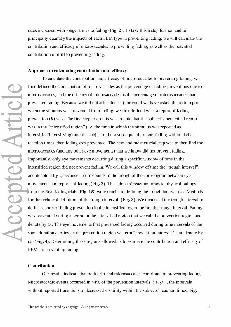
rates increased with longer times to fading (Fig. 2). To take this a step further, and to

principally quantify the impacts of each FEM type in preventing fading, we will calculate the

contribution and efficacy of microsaccades to preventing fading, as well as the potential

contribution of drift to preventing fading.

Approach to calculating contribution and efficacy

To calculate the contribution and efficacy of microsaccades to preventing fading, we

first defined the contribution of microsaccades as the percentage of fading preventions due to

microsaccades, and the efficacy of microsaccades as the percentage of microsaccades that

prevented fading. Because we did not ask subjects (nor could we have asked them) to report

when the stimulus was prevented from fading, we first defined what a report of fading

prevention (R) was. The first step to do this was to note that if a subject’s perceptual report

was in the “intensified region” (i.e. the time in which the stimulus was reported as

intensified/intensifying) and the subject did not subsequently report fading within his/her

reaction times, then fading was prevented. The next and most crucial step was to then find the

microsaccades (and any other eye movements) that we know did not prevent fading.

Importantly, only eye movements occurring during a specific window of time in the

intensified region did not prevent fading. We call this window of time the “trough interval”,

and denote it by , because it corresponds to the trough of the correlogram between eye

movements and reports of fading (Fig. 3). The subjects’ reaction times to physical fadings

from the Real fading trials (Fig. 1B) were crucial to defining the trough interval (see Methods

for the technical definition of the trough interval) (Fig. 3). We then used the trough interval to

define reports of fading prevention in the intensified region before the trough interval. Fading

was prevented during a period in the intensified region that we call the prevention region and

denote by . The eye movements that prevented fading occurred during time intervals of the

same duration as inside the prevention region we term "prevention intervals", and denote by

i (Fig. 4). Determining these regions allowed us to estimate the contribution and efficacy of

FEMs to preventing fading.

Contribution

Our results indicate that both drift and microsaccades contribute to preventing fading.

Microsaccadic events occurred in 44% of the prevention intervals (i.e. i , the intervals

without reported transitions to decreased visibility within the subjects’ reaction times; Fig.


5A), and in only 3% of the trough intervals (i.e. , intervals preceding reports of decreased

visibility within the reaction times of the subjects). The difference between these two

quantities (41%) provides a lower bound on the contribution of microsaccades, ( ),R M to

preventing fading (Fig. 5B). That is, microsaccades caused a minimum of 41% and a

maximum of 44% of all fading preventions.

Drift is ever-present (Cornsweet, 1956), thus drift occurred in essentially every

prevention interval and every trough interval. Due to the continuous nature of drift, one

cannot determine its contribution and efficacy in the same manner as with transient eye

movements such as microsaccades, saccades, and blinks. We defined drift alone (D) as the

event that only drift occurred over an interval of time with duration equal to 's duration. The

probability of drift alone in a prevention interval i, was 52%, placing an upper bound on the

contribution of drift alone to preventing visual fading (this upper bound did not vary

significantly with eccentricity; data not shown). In other words, drift alone caused a

maximum of 52% of all fading preventions (Fig. 5A). This suggests that, whereas the

contribution of drift to the reversal of fading is small (McCamy et al., 2012), drift alone is a

large contributor to preventing fading. Thus, the low contribution of drifts to the reversal of

fading does not preclude its playing a larger role in the prevention of fading; indeed, it is

possible that drift is more important than microsaccades to preventing fading.

Efficacy

The efficacy of microsaccades, ( ),R M was 88%; that is, 88% of the microsaccadic

events that occurred during a period of intensification prevented fading (Fig. 5C). Saccadic

efficacy , ( ),R S (89%) and microsaccadic efficacy were similar (Fig. 5C). The efficacy of

any combination of microsaccades, saccades, and blinks (i.e. M, S, B, MS, MB) ranged from

87-92%, indicating that fading is rare in the presence of abrupt eye movements.

Neither the contribution nor the efficacy of microsaccades varied significantly as a

function of stimulus eccentricity (data not shown).

The efficacy of drift alone is difficult to get at, because of drift’s continuous nature. If

we simply applied our efficacy formula to drift alone, then we would get an efficacy of zero.

It could be that some drifts are better than others for preventing fading, and so it is not

appropriate to equate all drift alone events. It is important to remember that only the ocular

events that occurred within the prevention region -- but not the ocular events that occurred

within the trough interval -- prevented fading. Our results show that 97% of trough intervals


contained drift alone (i.e. 97% of fading reports were preceded by drift alone in the trough

interval), whereas only 52% of the prevention intervals contained drift alone. Thus, drift

alone was able to prevent fading in some cases, but not in others. Because of this, we

wondered whether drift alone in trough intervals was different (i.e. possibly slower) from

drift alone in the prevention intervals.


Drift and microsaccades in the trough intervals vs. prevention intervals

Drift .To compare drift inside the trough to drift in the prevention region, we

compared the mean, maximum, and standard deviation of the instantaneous drift speed inside

of trough intervals to those in the prevention intervals. We analyzed only drifts that occurred

in trough/prevention intervals without microsaccades/saccades or blinks. Furthermore,

because there are higher microsaccade rates in the prevention region than in the trough

interval (Fig. 3B), edge effects due to filtering can artificially change drift speeds between the

two regions (Fig. 6B), so we made comparisons after removing the edge effects due to the

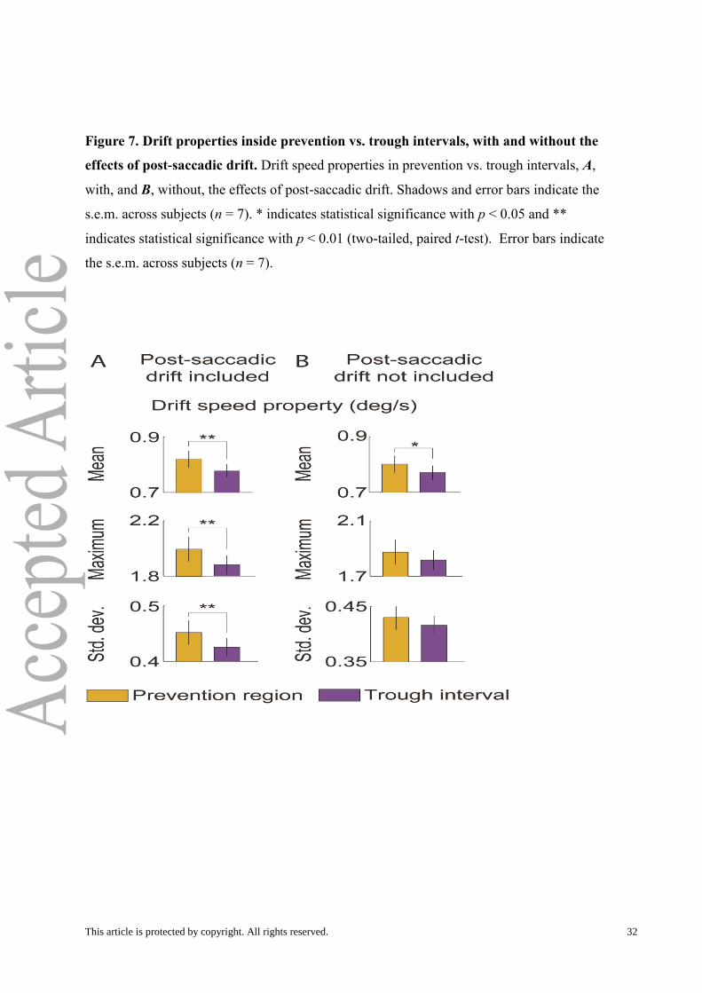
filter (see Methods; Fig. 6C-D). We found that all three parameters (i.e. mean, maximum, and

standard deviation) of instantaneous drift speed were larger on average inside the prevention

intervals than in the trough intervals (Fig. 7A), suggesting that faster drifts and drifts with

more variation in speed are better at preventing fading.

We wondered whether this result might be mainly due to increased post-saccadic drift

speeds after (micro)saccades (Chen and Hafed, 2013); Fig. 6C), To find out, we increased the

window after the beginning of the drift to get rid of the correlation of (micro)saccades (i.e.

post-saccadic drift; see Methods) and we analyzed only drift in prevention/trough intervals

that did not contain (micro)saccades or blinks. This approach ensured that the results would

not be explained by increased post-saccadic drift in the prevention region (Fig. 6C-D). In this

case, only the mean speed of drift was significantly, although moderately, faster in the

prevention intervals than in the trough intervals (Fig. 7B).

We note that removing the edge effects due to the filter was critical to our analyses,

because microsaccade rates differed between prevention and trough regions compared in Fig

7. If filter edge effects had remained, we would have obtained artificial results, because the

increased numbers of microsaccades in the prevention region would have resulted in more

instances of higher drift speeds. A similar argument applies to the post-saccadic drift. Given


that drifts seem to be faster in prevention intervals compared to the trough intervals, we

wondered whether microsaccade properties also differed between the two regions.


Microsaccade magnitude, number, and direction. Because the probability of a

microsaccade occurring in the trough interval is so low (3% of trough intervals had one or

more microsaccades) we suspected that the efficacy of microsaccades would not change with

different types of microsaccadic events. Upon doing the calculations, this is mostly what we

found; that is, microsaccades were equally effective at preventing fading independent of their

size and direction (Fig. 8A,C-D). In fact, the smallest microsaccades were just as effective as

large saccades at preventing fading. This is in extreme contrast to the role of microsaccades

in reversing fading, where microsaccadic efficacy increased linearly with microsaccade

magnitude, and multiple microsaccades were more effective at reversing fading than isolated

microsaccades (McCamy et al., 2012). Here, microsaccadic events with two or more

microsaccades were slightly, but significantly, more effective than microsaccadic events with

just one microsaccade (Fig. 8B).


DISCUSSION

Even when we attempt to fixate our gaze, small eye movements, called fixational eye

movements (FEMs: including microsaccades, drift and tremor) continue to shift our eye

position. Here we determined the role of FEMs in the prevention of visual fading during

fixation, for the first time, and found that both drift and microsaccades contribute to

preventing fading. Our results indicate that the contribution of drift to preventing fading is

potentially higher than that of microsaccades, but that microsaccades of any size prevent

fading with higher efficacy than drift, both in the visual periphery and in the fovea.

Microsaccades of all directions were equally effective at preventing fading, but two or more

microsaccades occurring in close succession were slightly (5%) more efficacious than single

microsaccades. We also found that drift was faster and had more variation in prevention

intervals (i.e. intervals without reported transitions to decreased visibility within the subjects’

reaction times) compared to trough intervals (i.e. intervals preceding reports of decreased

visibility within the subjects’ reaction times), but most of these differences were due to the

combination of increased post-saccadic drift speeds and higher microsaccade rates in

prevention intervals compared to trough intervals.


Our findings are compatible with a pioneering study by Gerrits and Vendrick, where

simulated drift and/or microsaccadic motions were imposed on parafoveal stimuli otherwise

stabilized on the retina (Gerrits and Vendrik, 1974). Based on qualitative analyses, the

authors concluded that “[…] the most effective eye movement to preserve vision is better

characterized by its qualities (irregularity and continuity) than by its name (drift or saccade)”

and that “[…] both the irregularity (the continuous change of direction) and the continuity of

the movement of a stimulus with respect to the retina are very important for the preservation

of perception.” Gerrits and Vendrick stressed that microsaccades were of minor importance

to visibility, however, in light of previous (albeit qualitative) work suggesting that

microsaccades were not needed to preserve foveal vision during maintained fixation. Gerrits

and Vendrick also proposed that Gaussian noise (drift) interspersed with binary noise

(microsaccades) resulted in very long periods of visibility, suggesting that the combination of

drift and microsaccades could optimize visibility during fixation, as indeed our present data

indicates. Our conclusion that microsaccades and drift both prevent fading is also consistent

with the finding (Engbert and Kliegl, 2004) that microsaccades and drift together provide

motion that is continuous (persistent on a short time scale) and irregular (anti-persistent on a

long time scale), also in line with Gerrits and Vendrick’s predictions.

Preventing vs. restoring faded vision

There has been much confusion about, and misuse of, the concepts of preventing and

reversing visual fading in the literature. Indeed, many previous papers have used both terms

as synonyms (Poletti and Rucci, 2010; Kagan, 2012) or failed to differentiate one from the

other (Nachmias, 1961; Sharpe, 1972; Kowler and Steinman, 1979). The present research

indicates that different constellations of eye movements mediate the prevention and the

reversal of visual fading during fixation. The combined results from the current study and our

previous research on the contribution and efficacy of FEMs to restoring faded vision

(McCamy et al., 2012) suggest that, whereas microsaccades are critical to counteracting

fading once it has happened, both drift and microsaccades synergistically prevent fading from

occurring. It may be that drift effectively prevents fading for a limited time only: that is, that

if a saccade, microsaccade, or blink does not interrupt the drift, then fading will occur

eventually. This notion is supported by the fact that drift alone occurred in 97% of trough

intervals: intervals preceding reports of decreased visibility within the reaction times of the

subjects. These findings may help to reconcile the long-standing controversy concerning the

comparative roles of microsaccades and drift in visibility during fixation.


Underlying physiology. Neural adaptation has been shown to occur at fast and slow

time scales (Sanchez-Vives et al., 2000a, 2000b; Wang et al., 2003) in the primary visual

cortex. One possible physiological explanation of the present perceptual results (as well as

those reported by (McCamy et al., 2012)) is that microsaccades reverse fast adaptation and

reverse/prevent slow adaptation, while drifts prevent/reverse slow adaptation. Because drift

moves visual receptive fields slowly over a small region of space, it may be that drift does not

work fast enough to reverse fast adaptation. In other words, because natural scenes are highly

correlated in space (Simoncelli and Olshausen, 2001), it follows that new stimuli brought into

receptive fields of visual neurons by drift are highly correlated to recent previous stimuli in

those same receptive fields. Conversely, because of the larger distance covered by

microsaccades, new stimuli entering the receptive fields of visual neurons will be less likely

correlated to recent stimuli. Future research should investigate the possibility that transient

signals due to microsaccades combine with sustained signals due to drifts to produce optimal

visual stimulation.

Enhancement vs. suppression. It is widely believed that microsaccades come with

elevated perceptual thresholds (Zuber and Stark, 1966; Beeler, 1967), but see (Krauskopf et

al., 1966). This elevation does not preclude a perceptual benefit of microsaccades, however.

Microsaccades act to move a visual stimulus to a new location on the retina. Once

suppression has occurred, that act can still be beneficial to perception by causing transient

stimulation, followed by increased sustained responses (enhanced by drift). Even square-

wave jerks (SWJs), which are consecutive microsaccades that occur in opposite directions

(Martinez-Conde, 2006; Chen et al., 2010; Otero-Millan et al., 2011, 2013; McCamy et al.,

2013), may be perceptually advantageous; for instance if the brief movement caused by the

first saccade, followed by the quick return to the initial position by the second saccade of the

SWJ (usually within ~200 ms), provides enough time for a brief recovery from neural

adaptation.


REFERENCES

Aertsen AM, Gerstein GL, Habib MK, Palm G (1989) Dynamics of neuronal firing

correlation: modulation of “effective connectivity.” J Neurophysiol 61:900–917.

Alonso J-M, Usrey WM, Reid RC (1996) Precisely correlated firing in cells of the lateral

geniculate nucleus. Nature 383:815–819.

Alonso J-M, Usrey WM, Reid RC (2001) Rules of connectivity between geniculate cells and

simple cells in cat primary visual cortex. J Neurosci 21:4002–4015.

Beeler (1967) Visual threshold changes resulting from spontaneous saccadic eye movements.

Vision research 7:769–775.

Chen AL, Riley DE, King SA, Joshi AC, Serra A, Liao K, Cohen ML, Otero-Millan J,

Martinez-Conde S, Strupp M, Leigh RJ (2010) The disturbance of gaze in progressive

supranuclear palsy: implications for pathogenesis. Front Neur 1:147.

Chen C-Y, Hafed ZM (2013) Postmicrosaccadic Enhancement of Slow Eye Movements. J

Neurosci 33:5375–5386.

Cornsweet TN (1956) Determination of the stimuli for involuntary drifts and saccadic eye

movements. J Opt Soc Am 46:987–988.

Costela FM, McCamy MB, Macknik SL, Otero-Millan J, Martinez-Conde S (2013)

Microsaccades restore the visibility of minute foveal targets. PeerJ 1:e119.

Di Stasi LL, McCamy MB, Catena A, Macknik SL, Cañas JJ, Martinez-Conde S (2013)

Microsaccade and drift dynamics reflect mental fatigue. European Journal of

Neuroscience 38:2389–2398.

Ditchburn RW, Ginsborg BL (1952) Vision with a Stabilized Retinal Image. Nature 170:36–

37.

Engbert R (2006) Microsaccades: A microcosm for research on oculomotor control, attention,

and visual perception. Prog Brain Res 154:177–192.

Engbert R, Kliegl R (2003) Microsaccades uncover the orientation of covert attention. Vision

Res 43:1035–1045.

Engbert R, Kliegl R (2004) Microsaccades keep the eyes’ balance during fixation. Psychol

Sci 15:431–436.

Engbert R, Mergenthaler K (2006) Microsaccades are triggered by low retinal image slip.

Proc Natl Acad Sci USA 103:7192–7197.

Gerrits HJM, Vendrik AJH (1974) The influence of stimulus movements on perception in

parafoveal stabilized vision. Vision Research 14:175–IN1.

Grun S (2009) Data-driven significance estimation for precise spike correlation. J

Neurophysiol 101:1126–1140.


Kagan I (2012) Microsaccades and image fading during natural vision. The Journal of

Neuroscience eLetters.

Kapoula Z, Robinson DA, Hain TC (1986) Motion of the eye immediately after a saccade.

Exp Brain Res 61:386–394.

Kowler E, Steinman RM (1979) Miniature saccades: Eye movements that do not count.

Vision Research 19:105–108.

Krauskopf J, Cornsweet TN, Riggs LA (1960) Analysis of eye movements during monocular

and binocular fixation. J Opt Soc Am 50:572.

Krauskopf J, Graf V, Gaarder K (1966) Lack of Inhibition during Involuntary Saccades. The

American Journal of Psychology 79:73–81.

Laubrock J, Engbert R, Kliegl R (2005) Microsaccade dynamics during covert attention.

Vision Res 45:721–730.

Levick WR, Cleland BG, Dubin MW (1972) Lateral geniculate neurons of cat: retinal inputs

and physiology. Invest Ophthalmol 11:302–311.

Martinez-Conde S (2006) Fixational eye movements in normal and pathological vision. In:

Visual Perception - Fundamentals of Vision: Low and Mid-Level Processes in

Perception, pp 151–176. Elsevier. Available at:

http://www.sciencedirect.com.ezproxy1.lib.asu.edu/science/article/B7CV6-4M0C546-

F/2/2321185cb4e661f44f2f859d714f5fbb [Accessed February 17, 2010].

Martinez-Conde S, Macknik SL, Hubel DH (2004) The role of fixational eye movements in

visual perception. Nat Rev Neurosci 5:229–240.

Martinez-Conde S, Macknik SL, Troncoso XG, Dyar TA (2006) Microsaccades counteract

visual fading during fixation. Neuron 49:297–305.

Martinez-Conde S, Otero-Millan J, Macknik SL (2013) The impact of microsaccades on

vision: towards a unified theory of saccadic function. Nature Reviews Neuroscience

14:83–96.

Mastronarde DN (1987) Two classes of single-input X-cells in cat lateral geniculate nucleus.

II. Retinal inputs and the generation of receptive-field properties. J Neurophysiol

57:381–413.

McCamy MB, Najafian Jazi A, Otero-Millan J, Macknik SL, Martinez-Conde S (2013) The

effects of fixation target size and luminance on microsaccades and square-wave jerks.

PeerJ 1:e9.

McCamy MB, Otero-Millan J, Macknik SL, Yang Y, Troncoso XG, Baer SM, Crook SM,

Martinez-Conde S (2012) Microsaccadic Efficacy and Contribution to Foveal and

Peripheral Vision. J Neurosci 32:9194–9204.

Møller F, Laursen M, Tygesen J, Sjølie A (2002) Binocular quantification and

characterization of microsaccades. Graefes Arch Clin Exp Ophthalmol 240:765–770.


Nachmias J (1961) Determiners of the drift of the eye during monocular fixation. Journal of

the Optical Society of America (1917-1983) 51:761.

Otero-Millan J, Schneider R, Leigh RJ, Macknik SL, Martinez-Conde S (2013) Saccades

during Attempted Fixation in Parkinsonian Disorders and Recessive Ataxia: From

Microsaccades to Square-Wave Jerks. PLoS ONE 8:e58535.

Otero-Millan J, Serra A, Leigh RJ, Troncoso XG, Macknik SL, Martinez-Conde S (2011)

Distinctive features of saccadic intrusions and microsaccades in progressive

supranuclear palsy. J Neurosci 31:4379 –4387.

Palm G, Aertsen AMHJ, Gerstein GL (1988) On the significance of correlations among

neuronal spike trains. Biological Cybernetics 59:1–11.

Poletti M, Rucci M (2010) Eye movements under various conditions of image fading. J Vis

10:1–18.

Reid RC, Alonso JM (1995) Specificity of monosynaptic connections from thalamus to visual

cortex. Nature 378:281–284.

Riggs LA, Ratliff F (1952) The effects of counteracting the normal movements of the eye.

Journal of the Optical Society of America 42:872–873.

Rolfs M, Laubrock J, Kliegl R (2006) Shortening and prolongation of saccade latencies

following microsaccades. Exp Brain Res 169:369–376.

Sanchez-Vives MV, Nowak LG, McCormick DA (2000a) Membrane Mechanisms

Underlying Contrast Adaptation in Cat Area 17 In Vivo. J Neurosci 20:4267–4285.

Sanchez-Vives MV, Nowak LG, McCormick DA (2000b) Cellular Mechanisms of Long-

Lasting Adaptation in Visual Cortical Neurons In Vitro. J Neurosci 20:4286–4299.

Sharpe CR (1972) The visibility and fading of thin lines visualized by their controlled

movement across the retina. J Physiol 222:113–134.

Simoncelli EP, Olshausen BA (2001) Natural image statistics and neural representation.

Annual Review of Neuroscience 24:1193–1216.

Troncoso XG, Macknik SL, Martinez-Conde S (2008) Microsaccades counteract perceptual

filling-in. J Vis 8:1–9.

Usrey WM, Reppas JB, Reid RC (1998) Paired-spike interactions and synaptic efficacy of

retinal inputs to the thalamus. Nature 395:384–387.

Usrey WM, Reppas JB, Reid RC (1999) Specificity and strength of retinogeniculate

connections. J Neurophysiol 82:3527–3540.

Wang X-J, Liu Y, Sanchez-Vives MV, McCormick DA (2003) Adaptation and Temporal

Decorrelation by Single Neurons in the Primary Visual Cortex. J Neurophysiol

89:3279–3293.


Yarbus AL (1957) The perception of an image fixed with respect to the retina.

Biophysics:683–690.

Yarbus AL (1967) Eye movements and vision. New York: Plenum press.

Zuber BL, Stark L (1966) Saccadic suppression: elevation of visual threshold associated with

saccadic eye movements. Experimental neurology 16:65–79.

ADDITIONAL INFORMATION

Competing interests

The authors declare no competing interests.

Author contributions

MBM, SLM, and SMC contributed to the conception and design of the study and to drafting

the article or revising it critically for important intellectual content. MBM conducted the data

analyses.

Funding

This study was supported by the Barrow Neurological Foundation (S.L.M. and S.M.-C.) and

National Science Foundation Awards 0852636 and 1153786 (S.M.-C.).

Acknowledgements

We thank B. Kousari for technical assistance.

TABLES

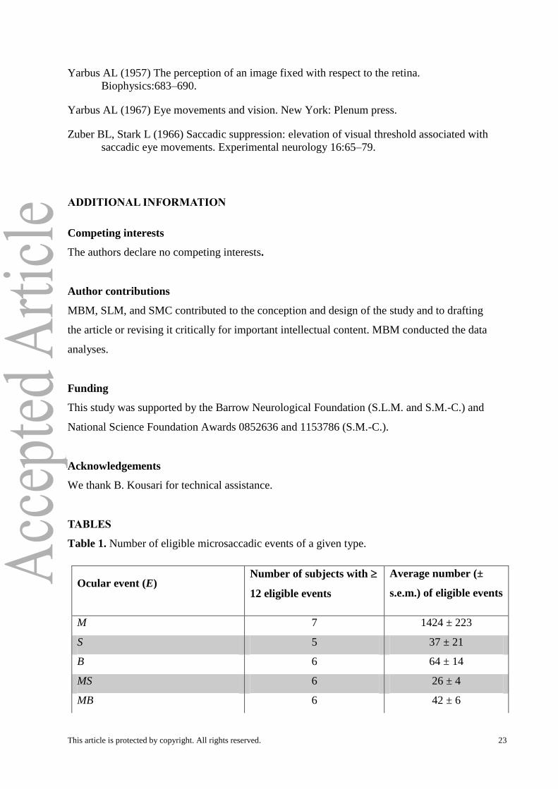
Table 1. Number of eligible microsaccadic events of a given type.

Ocular event (E) Number of subjects with

12 eligible events

Average number (±

s.e.m.) of eligible events

M 7 1424 ± 223

S 5 37 ± 21

B 6 64 ± 14

MS 6 26 ± 4

MB 6 42 ± 6


M1 (magnitude in [0, 0.25) deg) 6 295 ± 73

M2 (magnitude in [0.25, 0.5) deg) 7 860 ± 161

M3 (magnitude in [0.5, 0.75) deg) 7 296 ± 68

M4 (magnitude in [0.75, 1) deg) 6 64 ± 14

1M (one microsaccade) 7 1034 ± 143

2M ( two or more microsaccades) 7 391 ± 112

D (drift alone) 7 1932 ± 309

MC1 (C in [0 10) degrees) 7 62 ± 10

MC2 (C in [10 20) degrees) 7 76 ± 14

MC3 (C in [20 30) degrees) 7 71 ± 12

MC4 (C in [30 40) degrees) 7 88 ± 15

MC5 (C in [40 50) degrees) 7 90 ± 13

MC6 (C in [50 60) degrees) 7 85 ± 14

MC7 (C in [60 70) degrees) 7 74 ± 13

MC8 (C in [70 80) degrees) 7 78 ± 16

MC9 (C in [80 90) degrees) 7 93 ± 13

MC10 (C in [90 100) degrees) 7 93 ± 13

MC11 (C in [100 110) degrees) 7 71 ± 13

MC12 (C in [110 120) degrees) 7 71 ± 12

MC13 (C in [120 130) degrees) 7 86 ± 14

MC14 (C in [130 140) degrees) 7 108 ± 18

MC15 (C in [140 150) degrees) 7 90 ± 12

MC16 (C in [150 160) degrees) 7 82 ± 12

MC17 (C in [160 170) degrees) 7 85 ± 13


MC18 (C in [170 180) degrees) 7 71 ± 10

MO1 (O in [0 10) degrees) 7 68 ± 10

MO2 (O in [10 20) degrees) 7 134 ± 20

MO3 (O in [20 30) degrees) 7 166 ± 26

MO4 (O in [30 40) degrees) 7 221 ± 36

MO5 (O in [40 50) degrees) 7 283 ± 43

MO6 (O in [50 60) degrees) 7 220 ± 36

MO7 (O in [60 70) degrees) 7 171 ± 26

MO8 (O in [70 80) degrees) 7 142 ± 23

MO9 (O in [80 90) degrees) 7 60 ± 15

The efficacy calculations in Figs. 5C, 8 required that each subject had a minimum of twelve

occurrences per ocular event type.


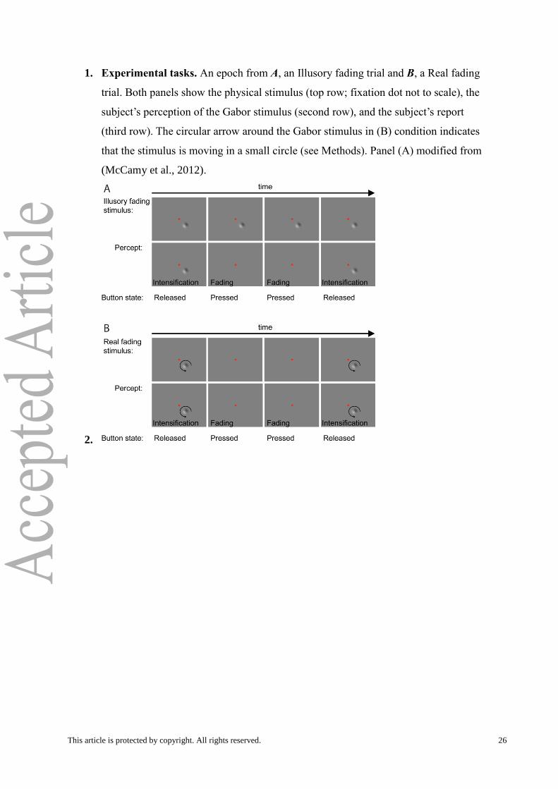
1. Experimental tasks. An epoch from A, an Illusory fading trial and B, a Real fading

trial. Both panels show the physical stimulus (top row; fixation dot not to scale), the

subject’s perception of the Gabor stimulus (second row), and the subject’s report

(third row). The circular arrow around the Gabor stimulus in (B) condition indicates

that the stimulus is moving in a small circle (see Methods). Panel (A) modified from

(McCamy et al., 2012).

2.


Figure 2. Time-to-fading. Microsaccade rates (i.e microsaccades per second; N/s) as a

function of how long the stimulus took to fade, i.e. microsaccade rates for intensification

periods of varying duration. Shadow indicates the s.e.m. across subjects (n = 7).


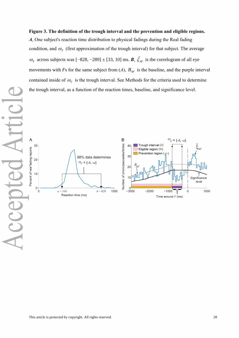
Figure 3. The definition of the trough interval and the prevention and eligible regions.

A, One subject's reaction time distribution to physical fadings during the Real fading

condition, and F (first approximation of the trough interval) for that subject. The average

F across subjects was [−828, −289] ± [33, 10] ms. B, AF is the correlogram of all eye

movements with Fs for the same subject from (A), AFB is the baseline, and the purple interval

contained inside of F is the trough interval. See Methods for the criteria used to determine

the trough interval, as a function of the reaction times, baseline, and significance level.


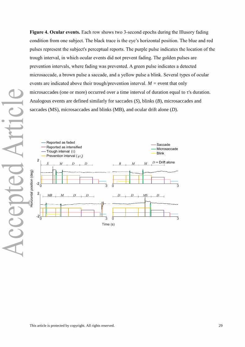
Figure 4. Ocular events. Each row shows two 3-second epochs during the Illusory fading

condition from one subject. The black trace is the eye’s horizontal position. The blue and red

pulses represent the subject's perceptual reports. The purple pulse indicates the location of the

trough interval, in which ocular events did not prevent fading. The golden pulses are

prevention intervals, where fading was prevented. A green pulse indicates a detected

microsaccade, a brown pulse a saccade, and a yellow pulse a blink. Several types of ocular

events are indicated above their trough/prevention interval. M = event that only

microsaccades (one or more) occurred over a time interval of duration equal to 's duration.

Analogous events are defined similarly for saccades (S), blinks (B), microsaccades and

saccades (MS), microsaccades and blinks (MB), and ocular drift alone (D).


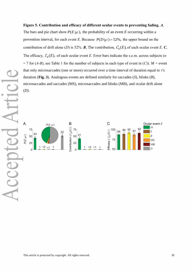
Figure 5. Contribution and efficacy of different ocular events to preventing fading. A,

The bars and pie chart show ( | ),P E the probability of an event E occurring within a

prevention interval, for each event E. Because ( | ) 52%,P D the upper bound on the

contribution of drift alone (D) is 52%. B, The contribution, ( ),R E of each ocular event E. C,

The efficacy, ( ),R E of each ocular event E. Error bars indicate the s.e.m. across subjects (n

= 7 for (A-B), see Table 1 for the number of subjects in each type of event in (C)). M = event

that only microsaccades (one or more) occurred over a time interval of duration equal to 's

duration (Fig. 3). Analogous events are defined similarly for saccades (S), blinks (B),

microsaccades and saccades (MS), microsaccades and blinks (MB), and ocular drift alone

(D).


Figure 6. Instant drift speed correlations with microsaccades and random

microsaccades. A-B, Instant drift speed around microsaccades (A) and random

microsaccades (B) with 10 ms windows removed from the beginning and end of each drift.

The changes in drift speed around the time of random microsaccades (decreases prior to and

increases after) are due to the edge effects of the filter. C-D, Instant drift speed around

microsaccades (C) and random microsaccades (D) with 34 ms removed from the beginning

and 110 ms removed from the end of each drift; thus removing the edge effects due to the

filter. Shadows indicate the s.e.m. across subjects (n = 7).


Figure 7. Drift properties inside prevention vs. trough intervals, with and without the

effects of post-saccadic drift. Drift speed properties in prevention vs. trough intervals, A,

with, and B, without, the effects of post-saccadic drift. Shadows and error bars indicate the

s.e.m. across subjects (n = 7). * indicates statistical significance with p < 0.05 and **

indicates statistical significance with p < 0.01 (two-tailed, paired t-test). Error bars indicate

the s.e.m. across subjects (n = 7).


Figure 8. Microsaccade magnitude, number, and direction. A, The efficacy of

microsaccadic and saccadic events did not vary significantly with magnitude. iM denotes the

microsaccadic event M whose magnitude falls in the interval [0.25( 1),0.25 )i i degrees, for

1, ,4.i B, Microsaccadic events M with two or more microsaccades 2( )M

were slightly,

but significantly, more efficacious than events with one microsaccade 1( )M . C, The efficacy

of microsaccades did not vary as a function of their direction relative to the compass position

of the Gabor. C is the angle between the microsaccade direction and the compass position of

the Gabor. CiM denotes the microsaccadic event M whose C falls in the interval

[10( 1),10 )i i degrees, for 1, ,18.i D, The efficacy of microsaccades did not vary as a

function of their direction relative to the orientation of the Gabor. O is the angle between the

microsaccade direction and the orientation of the Gabor. OiM denotes the microsaccadic

event M whose O falls in the interval [10( 1),10 )i i degrees, for 1, ,9.i Error bars

indicate the s.e.m. across subjects; see Table 1 for the number of subjects in each type of

event. * indicates statistical significance with p < 0.05 (two-tailed, paired t-test).

Documents

Authors: 1,2, Stephen L. Macknik1,3, Susana Martinez …smc.neuralcorrelate.com/files/publications/mccamy_jphysiology2014.pdf · This is an Accepted Article that has been peer-reviewed