AUT Journal of Mechanical Engineering

AUT Journal of Mechanical Engineering

AUT J. Mech. Eng., 2(2) (2018) 207-216DOI: 10.22060/ajme.2018.13711.5692

Fault Analysis of Complex Systems via Dynamic Bayesian Network

M. A. Farsi

Aerospace Research Institute, Ministry of science, research and technology, Tehran, Iran

ABSTRACT: Nowadays, several components and systems are designed and produced based on reliability. Since the reliability criterion has an important role in purchasing and implementation of these systems. In the design of a reliable system, fault and failure analysis must be carried out in order to reduce fault probability of the system. When dependency and the relation between components of a complex system are important and should be mentioned, determination of system reliability is very difficult. In this paper, dynamic fault tree is used to evaluate the systems reliability that their behavior is varied with time. Dynamic fault tree is constructed and then it converted to dynamic bayesian network. In this paper, the principle of dynamic fault tree gates and their mapping into dynamic bayesian are explained and some new relations between events and gates for this mapping are proposed. GeNIe package is used to determine dynamic bayesian network based on stochastic sampling algorithms. Four systems (cardiac assist system, hypothetical cascaded priority-and system, inertial navigation system/ global positioning system integrated, and emergency detection system) are investigated; reliability and fault probability of these systems are calculated. Comparison of the results with those obtained by other researches shows the proposed method effectiveness for systems reliability modeling and assessment via dynamic bayesian network.

Review History:

Received: 14 November 2017Revised: 4 April 2018Accepted: 29 April 2018Available Online: 15 May 2018

Keywords:

Dynamic fault treeDynamic bayesian networkDynamic systemReliability

207

1- IntroductionWhen a new system is developed, the system reliability evaluation should be carried out in order to determine whether the system is acceptable for an actual application. Reliability of systems are analyzed to compare with requirements and regulatory criteria designed to ensure the availability of high-quality qualifications. The failure probability of component in advanced industries is very small, but when it occurs the mission may be failed.There are several methods for reliability analysis: reliability block diagrams, the fault tree, event tree method, failure mode and effect analysis, Petri net, Markov chains, and Monte Carlo simulation. Each method has its own unique features and those features should be heeded when a system is investigated and analyzed [1].In an advanced industry such as aerospace industry, several digital systems are developed and used. The Reliability modeling and assessment of these systems are very important since reliability criterion has a vital role in using and implementation of these systems. When the conventional static modeling and evaluation methods, such as the block diagram, event tree, master logic diagram and fault tree method, present significant shortcomings used in the reliability modeling of digital instrumentation and control (I&C) systems in the industry, they cannot properly account for dynamic interactions between the digital systems and components [2]. Also, several systems in the aerospace industry should work based on the fault tolerant method. In these systems, fault detection and covering are very important. Also, time-dependent probabilistic models to predict system performance and cost consideration are necessary. Based on this matter, redundancy (cold, warm and hot), and function

dependent units are frequently used. In this condition, the system behavior is dynamic and it should be analyzed via dynamic methods. To overcome the limitations of the conventional static modeling, dynamic modeling methods should be implied for the reliability assessment. Dynamic Fault Trees (DFTs) were developed primarily to capture the complex dynamic behavior of the failure mechanisms of fault-tolerant systems and other dynamic systems. For example, Salehpour and Pourgol Mohammad studied on a dynamic system (steam turbine) and model its behavior [3]. They used Priority-AND (PAND) gate for system modeling and improve that system fault diagnosis. DFTs are traditionally solved using Markov chain analysis techniques, based on the specification and modeling of the whole set of possible states of the system and the transitions between them. Consequently, the state-space generated, grows exponentially with the number of components in the system, with a concomitant influence on computation times. Furthermore, the failure times of the system components to be modeled as exponentially distributed variables in Markov chain based approaches [4]. This makes DFTs much too inflexible for analyzing general standby redundant systems. To overcome the limitations of the Markov chain technique, several methods such as Petri Net, dynamic Reliability Block Diagram, Monte Carlo simulation and Bayesian Networks (BNs) are developed by researchers.In the past decade, BN was applied to modeling dependency in reliability and Risk engineering. At the first time, BN was introduced to a static system, but it extended and widely implied in dynamic system modeling [5]. Recently, several researchers have tried to develop this method to time-dependent modeling known as Dynamic Bayesian Networks (DBNs) [6], they offer a unified framework for reliability Corresponding author, E-mail: [email protected]

M. A. Farsi, AUT J. Mech. Eng., 2(2) (2018) 207-216, DOI: 10.22060/ajme.2018.13711.5692

208

modeling and analysis of complex dynamic systems. BNs have been used to increase the modeling capabilities and analysis power of DFT, including new features like general component failure distributions, multi-state variables, noisy gates, common cause failures, and simple sequentially dependent failures [4]. In initial researches, BN was converted to Markov change model and then it was solved [7, 8]. In this condition, the solver is influenced by Markov method limitations such as state exploration. Considering the above-mentioned problems encountered in converting DFT into Markov change model, temporal Bayesian networks (TBNs) have alternatively been proposed to explicitly incorporate time in the modeling of sequential dependencies without resort to Markov change. Accordingly, two different approaches have been adopted: Instant-based (time-sliced) approach and interval -based (event-based) approach [9].Several researchers have worked on BN and the application of this to modeling and evaluation of reliability and risk in the industry [10-15]. Also, in several works, BN has been used to model and solve diagnostic and maintenance problems [16, 17]. Although, several methods for construction of a BN and mapping a DFT into a DBN have been proposed; to increase capability and accuracy of methods and to overcome their limitations, work and study on this filed will be continued. Li et al. [18] used the fuzzy numbers as input data for a dynamic gate for the system reliability evaluation based on the BN. They alleviate the state space explosion problem involving in the latter studies.In this paper, the instant-based approach is implied. The relations of some dynamic gates for mapping DFT to DBN are developed, and GeNIe package is used to define the dynamic gates mapping and determine the probability of failure in complex systems. To demonstrate effectiveness and capability of this method to solve DFT, several examples are investigated and compared with other researcher’s results. In the next sections, the principle of BN is explained, then DBN and dynamic gates mapping into DBN are described.

2- Bayesian NetworkBN is a directed acyclic graph for reasoning under uncertainty in which the nodes represent variables and are connected by means of direct arcs. The arcs show causal relationship or dependencies between the linked nodes (parent nodes), and the Conditional Probability Tables (CPT) determine how the linked nodes are dependent on each other [9]. A simple BN is shown in Fig. 1. This BN includes three nodes and two arcs. For example, Node A and B are parent nodes for node C and Node C is a child for Nodes A and B. It is assumed that nodes A and B are independent.

The initialized Probability of C in this net calculated as follows (Eq. (1)):

( ) ( ) ( ) ( )( ) ( )

( )( )( )

( ) ( )( ) ( )( ) ( )( )

~ ~

~ ~ ( | )

( | ~ ) ~

( | ~ ) ~

( | ~ ~ ) ~ ~

( | )

( |~ ) ~

( | ~ ) ~

( | ~ ~ ) ~

Pr C Pr CAB Pr C AB Pr CA B

Pr C A B Pr C AB Pr AB

Pr C AB Pr AB

Pr C A B Pr A B

Pr C A B Pr A B

Pr C AB Pr A Pr B

Pr C AB Pr A Pr B

Pr C A B Pr A Pr B

Pr C A B Pr A

= + +

+ = ×

+ ×

+ ×

+ ×

= × ×

+ × ×

+ × ×

+ × ( )

( ) ( ) 1

( ) ( )

1

( ) ( ) 1

( ) ( ) 1

~

tT

T

pr triggerevent t triggerevent t active

pr triggerevent t active triggerevent t deactive

e

pr A t fail triggerevent t active

pr A t fail triggereve

Pr B

nt t deactive e

λ

λ

∆−

−

+ ∆ = = + ∆ = =

= −

= = =

= = = −

×

{ }

( ) ( ) , 1

( ) ( ), ( )

( 1)

( ) ( ) , ( )

1

Pr ( ) ( ) 1

P

t

tA

dep

pr A t fail A t fail triggerevent

pr A t fail A t triggerevent t active

P

pr A t fail A t working triggerevent t deactive

e

primery t fail primery t fail

λ

∆

∆−

+ ∆ = = = + ∆ = + ∆ =

= =

+ ∆ = = + ∆ =

= −

+ ∆ = = =

{ }{ }{ }

{ }

r ( ) ( ) 1

Pr ( ) ( ) 1

Pr ( ) ( ) tan , ( )

1Pr ( ) ( ) , ( )

1

p

b

b

t

t

primery t fail primery t working e

backup t fail backup t fail

backup t fail backup t s dby primery t working

ebackup t fail backup t working primery t fail

e

λ

λ

λ

− ∆

− ∆

−

+ ∆ = = = −

+ ∆ = = =

+ ∆ = = =

= −

+ ∆ = = =

= −

( ) ( ) 1

( ) ( ) 1

( ) ( ) 1

( ) ( ) 1

( ) ( ) , ( ) 1

( ) ( )

tA

tB

t

pr A t fail A t fail

pr A t fail A t working e

pr B t fail B t fail

pr B t fail B t working e

pr PAND t fail A t fail B t fail

pr PAND t fail A t

λ

λ

∆

∆

∆

−

−

+ ∆ = = =

+ ∆ = = = − + ∆ = = =

+ ∆ = = = − + ∆ = = + ∆ = =

+ ∆ = + ∆ =

( ):

, ( ) 1

( ) ( ) 1

( ) ( ) 1

( ) ( ) 1

( ) ( ) 1

( )

)

0

(

tA

fail B t fail



pr B t fail B t fa

Ot

il

pr B

herw

t working A t work

ise

ing

pr B t fail B t wo

Pr PAND t

λ ∆−

+ ∆ =

+ ∆ = =

+ ∆ = = =

+ ∆ = = = − + ∆ = = = + ∆ = = =

+ ∆ = = , ( ) 1

( ) ( ) , ( ) 1

( ) ( ) , ( )

[ ( )]

tBrking A t fail e

pr SEQ t fail A t fail B t fail

pr SEQ t fail A t fail B t working

pr B t

λ ∆− = = − + ∆ = = + ∆ = = + ∆ = = + ∆ =

= + ∆

(1)

where; Pr(~A)=1-Pr(A); Pr(~B)=1-Pr(B); Pr(~C)=1-Pr(C).

2- 1- Dynamic Bayesian NetIn a Dynamic Bayesian Network (DBN) nodes value and state can be changed with time. The timeline is divided into different time interval “slices” as the simplest way to the description of time dependence. A timeline (0 b] is divided into N interval and one complete static BN for each time interval is assigned [9, 17]. Time discretization is very important and to increase the accuracy of the calculation, the time steps should be small. An arc from the lower numbered interval to a higher numbered one is used to show the time relation between them. If the nodes for a slice at time t is dependent only on nodes from slice t-1, then we say that the DBN is a two-slice DBN [9]. For a general case, the dependencies and relations may be extended to any time slice in the past. The simple DBN is shown in Fig. 2. In this example, for any given slice, node C is completely determined by its parents (nodes A and B). The parent nodes A and B at any given slice depend on their value in the previous slice. An interslice arc is used to show the dependence of the nodes that are time dependent. In this work, we assume the timeline is divided into N equal interval. The N is selected for a mission duration of the system according to input data.

3- Dynamic Fault Tree GatesA DFT modeling technique was developed to handle the difficulties and problems in the reliability analysis and assessment of the complex systems such as fault-tolerant computer systems and prognostic modeling special when they are used in critical applications such as aerospace, nuclear power plant, and safety system. DFT is a useful tool to Fig. 1. A simple BN

Fig. 2. A simple DBN expanded over time slices


209

expand and upgrade existing models. Also, DFT application may reduce system unavailability [18]. In a DFT the special gates called dynamic gates should be implied to model a complex system behavior. Several dynamic gates were adopted in the conventional fault tree method. Each dynamic gate can declare each dynamic failure process that is related to the failure sequence of the system items. Engineers usually use four dynamic gates for system behavior modeling. These dynamic gates are functional-dependency (FDEP) gate, spare gate (cold spare (CSP) gate, hot spare (HSP) gate, and warm spare (WSP) gate), PAND gate, and a sequence-enforcing (SEQ) gate [2, 15]. These gates in the next section are defined.

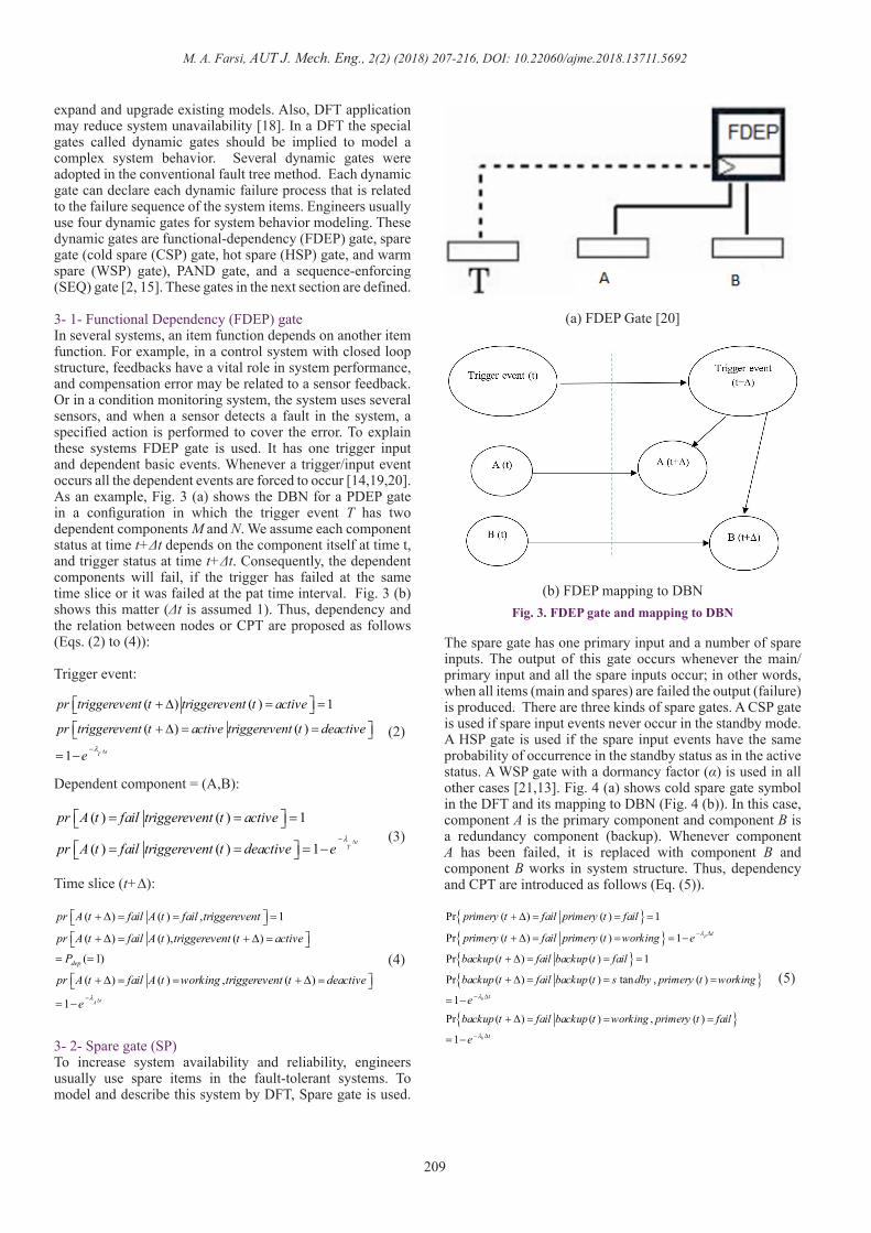
3- 1- Functional Dependency (FDEP) gateIn several systems, an item function depends on another item function. For example, in a control system with closed loop structure, feedbacks have a vital role in system performance, and compensation error may be related to a sensor feedback. Or in a condition monitoring system, the system uses several sensors, and when a sensor detects a fault in the system, a specified action is performed to cover the error. To explain these systems FDEP gate is used. It has one trigger input and dependent basic events. Whenever a trigger/input event occurs all the dependent events are forced to occur [14,19,20]. As an example, Fig. 3 (a) shows the DBN for a PDEP gate in a configuration in which the trigger event T has two dependent components M and N. We assume each component status at time t+Δt depends on the component itself at time t, and trigger status at time t+Δt. Consequently, the dependent components will fail, if the trigger has failed at the same time slice or it was failed at the pat time interval. Fig. 3 (b) shows this matter (Δt is assumed 1). Thus, dependency and the relation between nodes or CPT are proposed as follows (Eqs. (2) to (4)):

Trigger event:

( ) ( ) ( ) ( )( ) ( )

( )( )( )

( ) ( )( ) ( )( ) ( )( )

~ ~

~ ~ ( | )

( | ~ ) ~

( | ~ ) ~

( | ~ ~ ) ~ ~

( | )

( |~ ) ~

( | ~ ) ~

( | ~ ~ ) ~



Pr C AB Pr AB

Pr C A B Pr A B

Pr C A B Pr A B

Pr C AB Pr A Pr B

Pr C AB Pr A Pr B

Pr C A B Pr A Pr B

Pr C A B Pr A

= + +

+ = ×

+ ×

+ ×

+ ×

= × ×

+ × ×

+ × ×

+ × ( )

( ) ( ) 1

( ) ( )

1

( ) ( ) 1

( ) ( ) 1

~

tT

T



e



Pr B

nt t deactive e

λ

λ

∆−

−

+ ∆ = = + ∆ = =

= −

= = =

= = = −

×

{ }

( ) ( ) , 1

( ) ( ), ( )

( 1)

( ) ( ) , ( )

1

Pr ( ) ( ) 1

P

t

tA

dep



P


e


λ

∆

∆−

+ ∆ = = = + ∆ = + ∆ =

= =

+ ∆ = = + ∆ =

= −

+ ∆ = = =

{ }{ }{ }

{ }

r ( ) ( ) 1

Pr ( ) ( ) 1

Pr ( ) ( ) tan , ( )

1Pr ( ) ( ) , ( )

1

p

b

b

t

t





e

λ

λ

λ

− ∆

− ∆

−

+ ∆ = = = −

+ ∆ = = =

+ ∆ = = =

= −

+ ∆ = = =

= −

( ) ( ) 1

( ) ( ) 1

( ) ( ) 1

( ) ( ) 1

( ) ( ) , ( ) 1

( ) ( )

tA

tB

t






pr PAND t fail A t

λ

λ

∆

∆

∆

−

−

+ ∆ = = =

+ ∆ = = = − + ∆ = = =

+ ∆ = = = − + ∆ = = + ∆ = =

+ ∆ = + ∆ =

( ):

, ( ) 1

( ) ( ) 1

( ) ( ) 1

( ) ( ) 1

( ) ( ) 1

( )

)

0

(

tA

fail B t fail



pr B t fail B t fa

Ot

il

pr B

herw

t working A t work

ise

ing

pr B t fail B t wo

Pr PAND t

λ ∆−

+ ∆ =

+ ∆ = =

+ ∆ = = =

+ ∆ = = = − + ∆ = = = + ∆ = = =

+ ∆ = = , ( ) 1

( ) ( ) , ( ) 1

( ) ( ) , ( )

[ ( )]

tBrking A t fail e



pr B t

λ ∆− = = − + ∆ = = + ∆ = = + ∆ = = + ∆ =

= + ∆

(2)

Dependent component = (A,B):

( ) ( ) ( ) ( )( ) ( )

( )( )( )

( ) ( )( ) ( )( ) ( )( )

~ ~

~ ~ ( | )

( | ~ ) ~

( | ~ ) ~

( | ~ ~ ) ~ ~

( | )

( |~ ) ~

( | ~ ) ~

( | ~ ~ ) ~



Pr C AB Pr AB

Pr C A B Pr A B

Pr C A B Pr A B

Pr C AB Pr A Pr B

Pr C AB Pr A Pr B

Pr C A B Pr A Pr B

Pr C A B Pr A

= + +

+ = ×

+ ×

+ ×

+ ×

= × ×

+ × ×

+ × ×

+ × ( )

( ) ( ) 1

( ) ( )

1

( ) ( ) 1

( ) ( ) 1

~

tT

T



e



Pr B

nt t deactive e

λ

λ

∆−

−

+ ∆ = = + ∆ = =

= −

= = =

= = = −

×

{ }

( ) ( ) , 1

( ) ( ), ( )

( 1)

( ) ( ) , ( )

1

Pr ( ) ( ) 1

P

t

tA

dep



P


e


λ

∆

∆−

+ ∆ = = = + ∆ = + ∆ =

= =

+ ∆ = = + ∆ =

= −

+ ∆ = = =

{ }{ }{ }

{ }

r ( ) ( ) 1

Pr ( ) ( ) 1

Pr ( ) ( ) tan , ( )

1Pr ( ) ( ) , ( )

1

p

b

b

t

t





e

λ

λ

λ

− ∆

− ∆

−

+ ∆ = = = −

+ ∆ = = =

+ ∆ = = =

= −

+ ∆ = = =

= −

( ) ( ) 1

( ) ( ) 1

( ) ( ) 1

( ) ( ) 1

( ) ( ) , ( ) 1

( ) ( )

tA

tB

t






pr PAND t fail A t

λ

λ

∆

∆

∆

−

−

+ ∆ = = =

+ ∆ = = = − + ∆ = = =

+ ∆ = = = − + ∆ = = + ∆ = =

+ ∆ = + ∆ =

( ):

, ( ) 1

( ) ( ) 1

( ) ( ) 1

( ) ( ) 1

( ) ( ) 1

( )

)

0

(

tA

fail B t fail



pr B t fail B t fa

Ot

il

pr B

herw

t working A t work

ise

ing

pr B t fail B t wo

Pr PAND t

λ ∆−

+ ∆ =

+ ∆ = =

+ ∆ = = =

+ ∆ = = = − + ∆ = = = + ∆ = = =

+ ∆ = = , ( ) 1

( ) ( ) , ( ) 1

( ) ( ) , ( )

[ ( )]

tBrking A t fail e



pr B t

λ ∆− = = − + ∆ = = + ∆ = = + ∆ = = + ∆ =

= + ∆

(3)

Time slice (t+∆):

( ) ( ) ( ) ( )( ) ( )

( )( )( )

( ) ( )( ) ( )( ) ( )( )

~ ~

~ ~ ( | )

( | ~ ) ~

( | ~ ) ~

( | ~ ~ ) ~ ~

( | )

( |~ ) ~

( | ~ ) ~

( | ~ ~ ) ~



Pr C AB Pr AB

Pr C A B Pr A B

Pr C A B Pr A B

Pr C AB Pr A Pr B

Pr C AB Pr A Pr B

Pr C A B Pr A Pr B

Pr C A B Pr A

= + +

+ = ×

+ ×

+ ×

+ ×

= × ×

+ × ×

+ × ×

+ × ( )

( ) ( ) 1

( ) ( )

1

( ) ( ) 1

( ) ( ) 1

~

tT

T



e



Pr B

nt t deactive e

λ

λ

∆−

−

+ ∆ = = + ∆ = =

= −

= = =

= = = −

×

{ }

( ) ( ) , 1

( ) ( ), ( )

( 1)

( ) ( ) , ( )

1

Pr ( ) ( ) 1

P

t

tA

dep



P


e


λ

∆

∆−

+ ∆ = = = + ∆ = + ∆ =

= =

+ ∆ = = + ∆ =

= −

+ ∆ = = =

{ }{ }{ }

{ }

r ( ) ( ) 1

Pr ( ) ( ) 1

Pr ( ) ( ) tan , ( )

1Pr ( ) ( ) , ( )

1

p

b

b

t

t





e

λ

λ

λ

− ∆

− ∆

−

+ ∆ = = = −

+ ∆ = = =

+ ∆ = = =

= −

+ ∆ = = =

= −

( ) ( ) 1

( ) ( ) 1

( ) ( ) 1

( ) ( ) 1

( ) ( ) , ( ) 1

( ) ( )

tA

tB

t






pr PAND t fail A t

λ

λ

∆

∆

∆

−

−

+ ∆ = = =

+ ∆ = = = − + ∆ = = =

+ ∆ = = = − + ∆ = = + ∆ = =

+ ∆ = + ∆ =

( ):

, ( ) 1

( ) ( ) 1

( ) ( ) 1

( ) ( ) 1

( ) ( ) 1

( )

)

0

(

tA

fail B t fail



pr B t fail B t fa

Ot

il

pr B

herw

t working A t work

ise

ing

pr B t fail B t wo

Pr PAND t

λ ∆−

+ ∆ =

+ ∆ = =

+ ∆ = = =

+ ∆ = = = − + ∆ = = = + ∆ = = =

+ ∆ = = , ( ) 1

( ) ( ) , ( ) 1

( ) ( ) , ( )

[ ( )]

tBrking A t fail e



pr B t

λ ∆− = = − + ∆ = = + ∆ = = + ∆ = = + ∆ =

= + ∆

(4)

3- 2- Spare gate (SP)To increase system availability and reliability, engineers usually use spare items in the fault-tolerant systems. To model and describe this system by DFT, Spare gate is used.

The spare gate has one primary input and a number of spare inputs. The output of this gate occurs whenever the main/primary input and all the spare inputs occur; in other words, when all items (main and spares) are failed the output (failure) is produced. There are three kinds of spare gates. A CSP gate is used if spare input events never occur in the standby mode. A HSP gate is used if the spare input events have the same probability of occurrence in the standby status as in the active status. A WSP gate with a dormancy factor (α) is used in all other cases [21,13]. Fig. 4 (a) shows cold spare gate symbol in the DFT and its mapping to DBN (Fig. 4 (b)). In this case, component A is the primary component and component B is a redundancy component (backup). Whenever component A has been failed, it is replaced with component B and component B works in system structure. Thus, dependency and CPT are introduced as follows (Eq. (5)).

( ) ( ) ( ) ( )( ) ( )

( )( )( )

( ) ( )( ) ( )( ) ( )( )

~ ~

~ ~ ( | )

( | ~ ) ~

( | ~ ) ~

( | ~ ~ ) ~ ~

( | )

( |~ ) ~

( | ~ ) ~

( | ~ ~ ) ~



Pr C AB Pr AB

Pr C A B Pr A B

Pr C A B Pr A B

Pr C AB Pr A Pr B

Pr C AB Pr A Pr B

Pr C A B Pr A Pr B

Pr C A B Pr A

= + +

+ = ×

+ ×

+ ×

+ ×

= × ×

+ × ×

+ × ×

+ × ( )

( ) ( ) 1

( ) ( )

1

( ) ( ) 1

( ) ( ) 1

~

tT

T



e



Pr B

nt t deactive e

λ

λ

∆−

−

+ ∆ = = + ∆ = =

= −

= = =

= = = −

×

{ }

( ) ( ) , 1

( ) ( ), ( )

( 1)

( ) ( ) , ( )

1

Pr ( ) ( ) 1

P

t

tA

dep



P


e


λ

∆

∆−

+ ∆ = = = + ∆ = + ∆ =

= =

+ ∆ = = + ∆ =

= −

+ ∆ = = =

{ }{ }{ }

{ }

r ( ) ( ) 1

Pr ( ) ( ) 1

Pr ( ) ( ) tan , ( )

1Pr ( ) ( ) , ( )

1

p

b

b

t

t





e

λ

λ

λ

− ∆

− ∆

−

+ ∆ = = = −

+ ∆ = = =

+ ∆ = = =

= −

+ ∆ = = =

= −

( ) ( ) 1

( ) ( ) 1

( ) ( ) 1

( ) ( ) 1

( ) ( ) , ( ) 1

( ) ( )

tA

tB

t






pr PAND t fail A t

λ

λ

∆

∆

∆

−

−

+ ∆ = = =

+ ∆ = = = − + ∆ = = =

+ ∆ = = = − + ∆ = = + ∆ = =

+ ∆ = + ∆ =

( ):

, ( ) 1

( ) ( ) 1

( ) ( ) 1

( ) ( ) 1

( ) ( ) 1

( )

)

0

(

tA

fail B t fail



pr B t fail B t fa

Ot

il

pr B

herw

t working A t work

ise

ing

pr B t fail B t wo

Pr PAND t

λ ∆−

+ ∆ =

+ ∆ = =

+ ∆ = = =

+ ∆ = = = − + ∆ = = = + ∆ = = =

+ ∆ = = , ( ) 1

( ) ( ) , ( ) 1

( ) ( ) , ( )

[ ( )]

tBrking A t fail e



pr B t

λ ∆− = = − + ∆ = = + ∆ = = + ∆ = = + ∆ =

= + ∆

(5)

(a) FDEP Gate [20]

(b) FDEP mapping to DBNFig. 3. FDEP gate and mapping to DBN


210

3- 3- Priority-and gatePriority-and was commonly known as PAND gate. The PAND is used to show interactions between components of a complex system. For example, PAND gates model situations where a control component may prevent the system to crash (with ruinous consequences) because of the failure of a standard component. In such cases, a failure of the control component before the failure of the standard one prevents the recovery action of the control component, leading to a (sub) -system failure. The PAND gate has two inputs. The output of this gate occurs if and only if all input events occur in a particular order, or in other words when all items failed in a particular order. The order of occurrence that causes the output occurrence is from left to right. Thus we propose the PAND gate relations as following (Eq. (6)) and its mapping to DBN as Fig. 5 (b).

( ) ( ) ( ) ( )( ) ( )

( )( )( )

( ) ( )( ) ( )( ) ( )( )

~ ~

~ ~ ( | )

( | ~ ) ~

( | ~ ) ~

( | ~ ~ ) ~ ~

( | )

( |~ ) ~

( | ~ ) ~

( | ~ ~ ) ~



Pr C AB Pr AB

Pr C A B Pr A B

Pr C A B Pr A B

Pr C AB Pr A Pr B

Pr C AB Pr A Pr B

Pr C A B Pr A Pr B

Pr C A B Pr A

= + +

+ = ×

+ ×

+ ×

+ ×

= × ×

+ × ×

+ × ×

+ × ( )

( ) ( ) 1

( ) ( )

1

( ) ( ) 1

( ) ( ) 1

~

tT

T



e



Pr B

nt t deactive e

λ

λ

∆−

−

+ ∆ = = + ∆ = =

= −

= = =

= = = −

×

{ }

( ) ( ) , 1

( ) ( ), ( )

( 1)

( ) ( ) , ( )

1

Pr ( ) ( ) 1

P

t

tA

dep



P


e


λ

∆

∆−

+ ∆ = = = + ∆ = + ∆ =

= =

+ ∆ = = + ∆ =

= −

+ ∆ = = =

{ }{ }{ }

{ }

r ( ) ( ) 1

Pr ( ) ( ) 1

Pr ( ) ( ) tan , ( )

1Pr ( ) ( ) , ( )

1

p

b

b

t

t





e

λ

λ

λ

− ∆

− ∆

−

+ ∆ = = = −

+ ∆ = = =

+ ∆ = = =

= −

+ ∆ = = =

= −

( ) ( ) 1

( ) ( ) 1

( ) ( ) 1

( ) ( ) 1

( ) ( ) , ( ) 1

( ) ( )

tA

tB

t






pr PAND t fail A t

λ

λ

∆

∆

∆

−

−

+ ∆ = = =

+ ∆ = = = − + ∆ = = =

+ ∆ = = = − + ∆ = = + ∆ = =

+ ∆ = + ∆ =

( ):

, ( ) 1

( ) ( ) 1

( ) ( ) 1

( ) ( ) 1

( ) ( ) 1

( )

)

0

(

tA

fail B t fail



pr B t fail B t fa

Ot

il

pr B

herw

t working A t work

ise

ing

pr B t fail B t wo

Pr PAND t

λ ∆−

+ ∆ =

+ ∆ = =

+ ∆ = = =

+ ∆ = = = − + ∆ = = = + ∆ = = =

+ ∆ = = , ( ) 1

( ) ( ) , ( ) 1

( ) ( ) , ( )

[ ( )]

tBrking A t fail e



pr B t

λ ∆− = = − + ∆ = = + ∆ = = + ∆ = = + ∆ =

= + ∆

(6)

3- 4- Sequence enforcing gateSometimes an engineer to achieve the desired function, use sequencing operations and functions in the complex. As an example, in a fire safety system, smoke is detected by sensors and then this signal sends to the main computer, after processing an actuator is implied to perform the desired action. Sequence enforcing gate usually called SEQ gate. The SEQ gate forces input events to occur in a particular order, namely from left to right, and the output occurs when all the input events occur. Although the input events of a PAND gate can occur in any order, the input of a SEQ gate cannot occur before the occurrence of an input on the left side. Some researchers have assumed SEQ gate behavior is similar to CSP gate [13, 16]. In this paper, their method is used to SEQ gate modeling. Fig. 6 shows a SEQ gate and its mapping to DBN and CPT can be introduced as follows (Eq. (7)).

( ) ( ) ( ) ( )( ) ( )

( )( )( )

( ) ( )( ) ( )( ) ( )( )

~ ~

~ ~ ( | )

( | ~ ) ~

( | ~ ) ~

( | ~ ~ ) ~ ~

( | )

( |~ ) ~

( | ~ ) ~

( | ~ ~ ) ~



Pr C AB Pr AB

Pr C A B Pr A B

Pr C A B Pr A B

Pr C AB Pr A Pr B

Pr C AB Pr A Pr B

Pr C A B Pr A Pr B

Pr C A B Pr A

= + +

+ = ×

+ ×

+ ×

+ ×

= × ×

+ × ×

+ × ×

+ × ( )

( ) ( ) 1

( ) ( )

1

( ) ( ) 1

( ) ( ) 1

~

tT

T



e



Pr B

nt t deactive e

λ

λ

∆−

−

+ ∆ = = + ∆ = =

= −

= = =

= = = −

×

{ }

( ) ( ) , 1

( ) ( ), ( )

( 1)

( ) ( ) , ( )

1

Pr ( ) ( ) 1

P

t

tA

dep



P


e


λ

∆

∆−

+ ∆ = = = + ∆ = + ∆ =

= =

+ ∆ = = + ∆ =

= −

+ ∆ = = =

{ }{ }{ }

{ }

r ( ) ( ) 1

Pr ( ) ( ) 1

Pr ( ) ( ) tan , ( )

1Pr ( ) ( ) , ( )

1

p

b

b

t

t





e

λ

λ

λ

− ∆

− ∆

−

+ ∆ = = = −

+ ∆ = = =

+ ∆ = = =

= −

+ ∆ = = =

= −

( ) ( ) 1

( ) ( ) 1

( ) ( ) 1

( ) ( ) 1

( ) ( ) , ( ) 1

( ) ( )

tA

tB

t






pr PAND t fail A t

λ

λ

∆

∆

∆

−

−

+ ∆ = = =

+ ∆ = = = − + ∆ = = =

+ ∆ = = = − + ∆ = = + ∆ = =

+ ∆ = + ∆ =

( ):

, ( ) 1

( ) ( ) 1

( ) ( ) 1

( ) ( ) 1

( ) ( ) 1

( )

)

0

(

tA

fail B t fail



pr B t fail B t fa

Ot

il

pr B

herw

t working A t work

ise

ing

pr B t fail B t wo

Pr PAND t

λ ∆−

+ ∆ =

+ ∆ = =

+ ∆ = = =

+ ∆ = = = − + ∆ = = = + ∆ = = =

+ ∆ = = , ( ) 1

( ) ( ) , ( ) 1

( ) ( ) , ( )

[ ( )]

tBrking A t fail e



pr B t

λ ∆− = = − + ∆ = = + ∆ = = + ∆ = = + ∆ =

= + ∆

(7)

(a) CSP gate

(b) Spare gate mapping to DBNFig. 4. Spare gate and mapping to DBN [13]

(a) PAND gate

(b) PAND gate mapping to DBNFig. 5. PAND gate and mapping to DBN


211

4- ApplicationTo demonstration of the capability and accuracy of DBN and the proposed dynamic gates mapping to DBN, four case studies and examples are studied in this section.

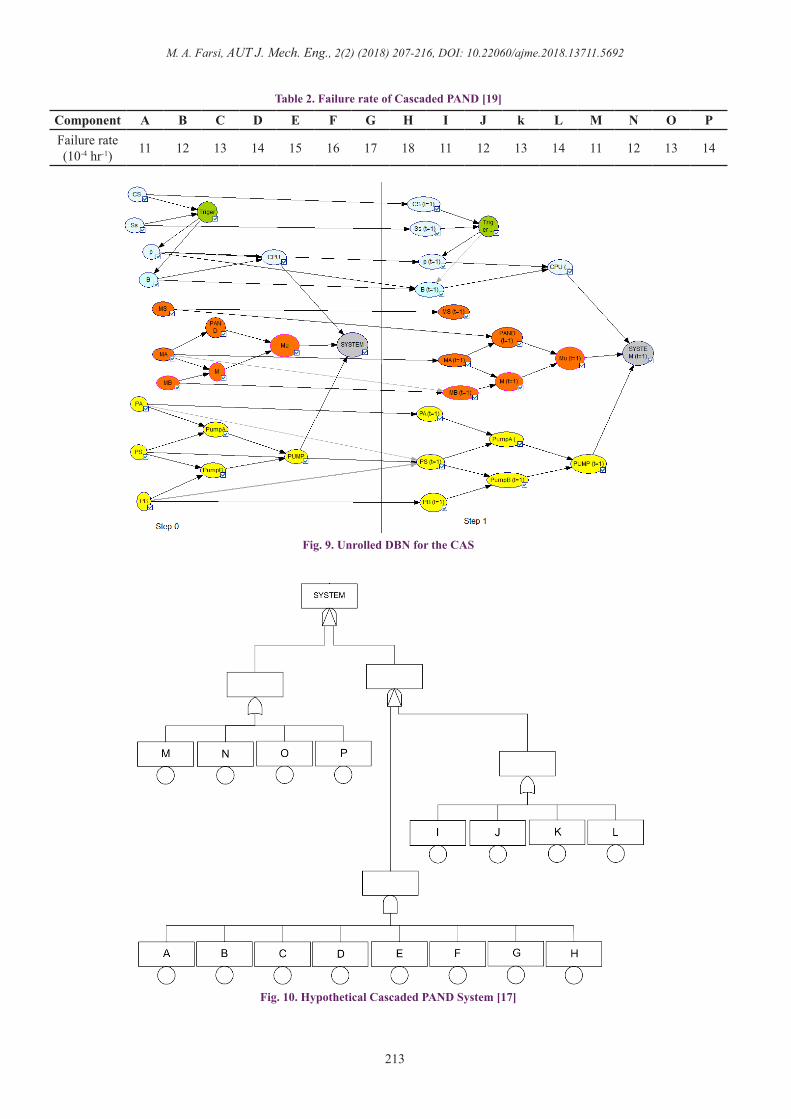
4- 1- Case 1Medical devices are often used to help the patient to reduce their problem and sickness. Cardiac Assist System (CAS) is one of the most important devices for heart disease. The reliability of this device is very important since the failure of this system lead to a ruinous consequence. The main sub-systems of a conventional CAS are CPU, Motor, and Pump. The failure of either one of these sub-system causes the whole system failure. Fig. 7 shows DFT proposed by Bobbio for a CAS [19,20]. In this case, to increase reliability, several spare components are used. For example, in CPU sub-system CPU P is the main CPU and B is warm spare CPU. These CPUs

are functionally depended on cross-switch (CS) and a system supervision (SS).The probability density function of all components is assumed as the exponential distribution. Table1 shows the failure rate for all components of this system. We will determine the reliability of this system for 1000 hours.At the first step, the DFT should be mapped to DBN. According to the proposed method in the previous sections, the DBN can be drawn same as Figs. 8 and 9 explains unrolled form (DBN on the timeline) for time slices. Time slice in this problem assumed 1 hour. The reliability of this system for 1000 hours is calculated using GeNie package and it is 0.66. This value same as result determined using Galileo and RADYBAN packages [20]. This result shows the accuracy of the mapping method that proposed in this paper.

(a) SEQ gate [13] (b) SEQ gate mapping to DBNFig. 6. SEQ gate mapping to DBN

Fig. 7. DFT of a CAS [20]


212

4- 2- Case 2The second case study is the Hypothetical Cascaded PAND System (HCPS). This system is shown as DFT in Fig. 10. This case was studied by several researchers to show the capability of their method [17, 19, 21,22]. We model this system and determine this system reliability.The proposed method result is compared with other packages and researchers results in table 3. According to this table, the proposed method is effective and powerful to determine this system reliability.

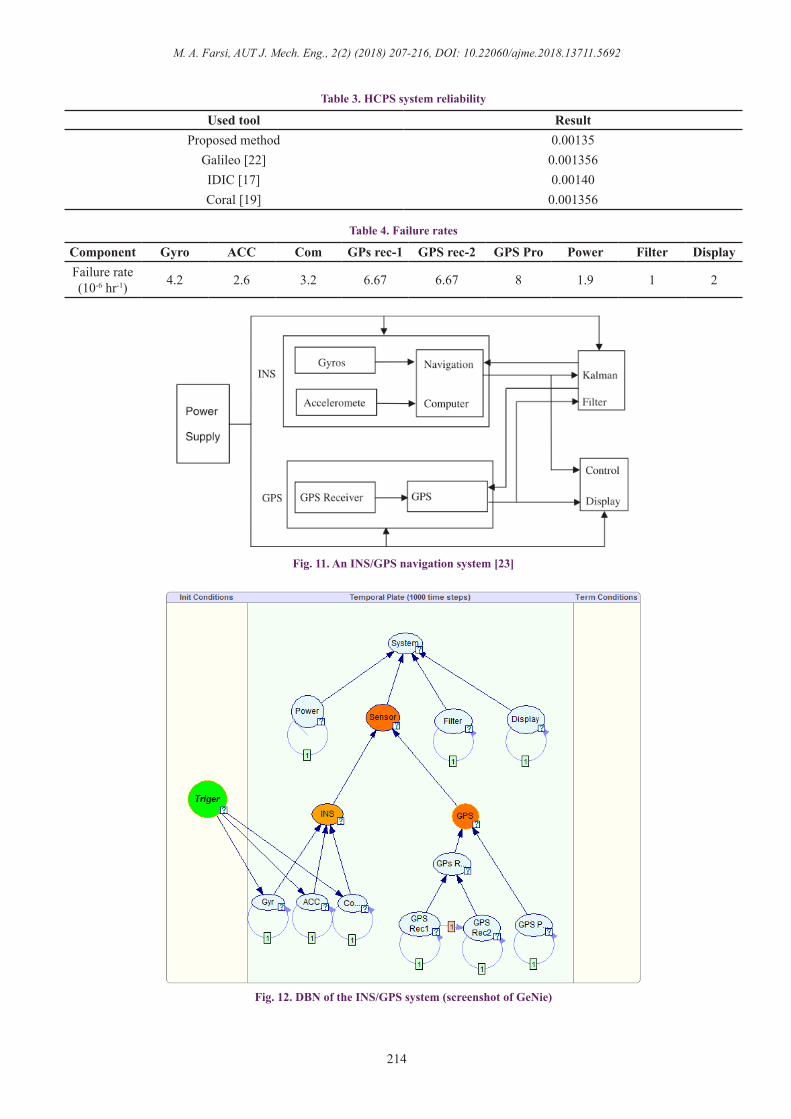
4- 3- Case 3In this section, the reliability of an Inertial Navigation System/Global Positioning System (INS/GPS) integrated navigation system, or simply the INS/GPS navigation system is determined. It consists of two or more different types of navigation equipment or sensors, and their outputs are obtained by fusing the multi-navigation information. Since several types of navigation equipment are used, the INS/GPS navigation system can meet a higher degree of precision with improved reliability from the redundant information in the system. Several configurations of the INS/GPS navigation systems exist depending on the application. In this paper, an INS/GPS is studied that it is presented in Fig. 11. The INS/GPS navigation system consists of four modules: power supply, sensors, a Kalman filter implemented on a computer and the control display. The sensor module of the INS includes gyros, accelerometers, and navigation computer, and for the GPS, the GPS receiver and processor [23]. In this system, an external sensor detects start time of moving and sends a signal to INS for reading data from its sensors. In other words, INS function depends on an external trigger. The DBN of the fault tree for this system is proposed as Fig. 12.In this system according to system structure, we assume the INS is a multi-state system. The INS output according to its sensors includes three states: success, failure and mild. In the mild state, the computer works, but one of gyros or accelerometer doesn’t work. Thus, the sensor module output includes three states: failure, success and half performance. In the half performance state, only one of the INS or GPS system works (these states were defined by the user and these may be modified by other users). Table 4 explains the component failure rate. Thus, the reliability of this system for 1000 hours flight equal to 0.99299. Also for Sensor module, the probability of failure state is 0.00011, the probability of success state is 0.9857, and the probability of half state is 0.01411.

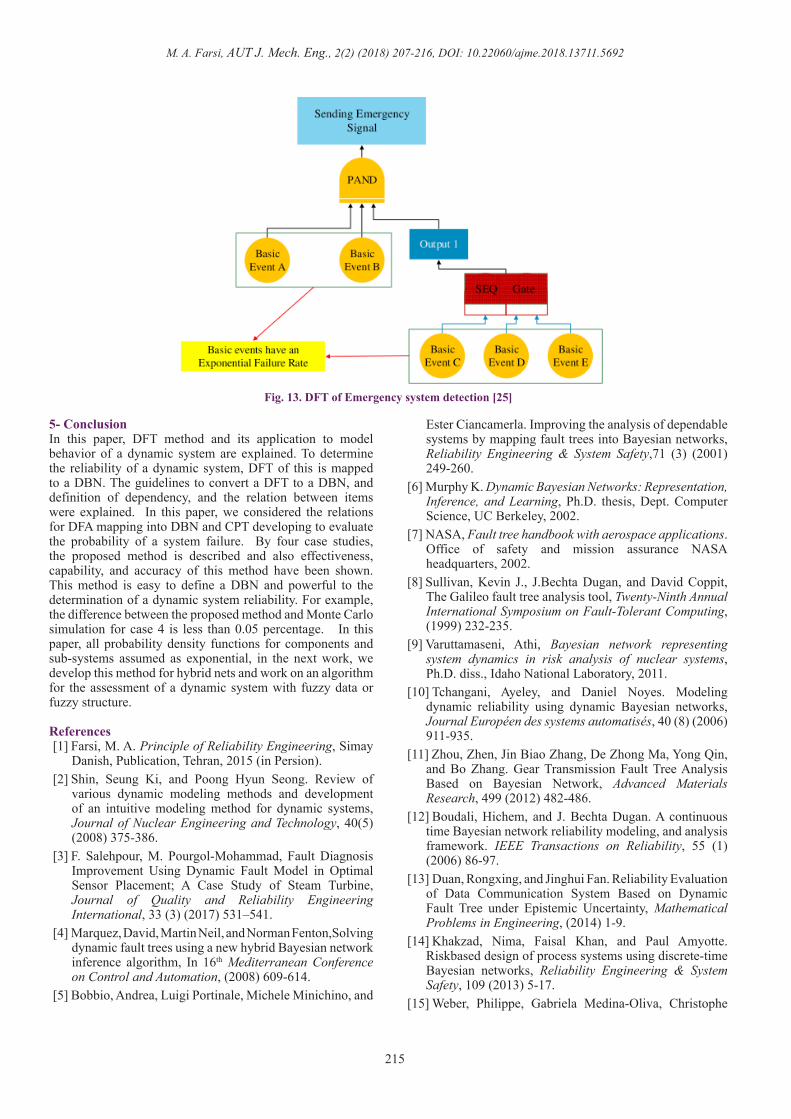
4- 4- Case 4An emergency detection system is studied as case 4. This system detects the emergency condition and sends a signal to the main flight control computer. Fig. 13 shows the emergency detection system DFT studied in this paper. This DFT consist of “Sending Emergency Signal” Top event and contains two dynamic PAND and SEQ gates. The PAND gate in addition with two basic events has an event from SEQ output. The output of PAND gate occurs when all events occurred in a specified order (left to right). In addition, SEQ gate of DFT has three BEs that events in this gate occur with the enforced sequenced order.If the failure rate is equal to 49.5E-6 for all components, the reliability of this system for 100 hours can be determined by DBN. The reliability of this system for 100 hours is determined as 0.9996. To evaluation of this result, this system was simulated using Monte Carlo method [25]. The reliability of the system using Monte Carlo simulation is 0.9991. The difference between the proposed method and Monte Carlo simulation is less than 0.05 percentage. Thus, it confirms our result and the proposed method for mapping DFT to DBN and determination of system reliability.

Comp. λ (1/h) αP 0.50E-3B 0.50E-3 0.5

CS 0.20E-3SS 0.20E-3MA 1.00E-3MB 1.00E-3 0MS 0.01E-3PA 1.00E-3PB 1.00E-3PS 1.00E-3 0

Table 1. Failure rate for the components of a CAS [20]

Fig. 8. DBN of the CAS (screenshot of GeNie)


213

Fig. 9. Unrolled DBN for the CAS

Fig. 10. Hypothetical Cascaded PAND System [17]

Component A B C D E F G H I J k L M N O PFailure rate(10-4 hr-1) 11 12 13 14 15 16 17 18 11 12 13 14 11 12 13 14

Table 2. Failure rate of Cascaded PAND [19]


214

Used tool ResultProposed method 0.00135

Galileo [22] 0.001356IDIC [17] 0.00140Coral [19] 0.001356

Table 3. HCPS system reliability

Fig. 11. An INS/GPS navigation system [23]

Fig. 12. DBN of the INS/GPS system (screenshot of GeNie)

Component Gyro ACC Com GPs rec-1 GPS rec-2 GPS Pro Power Filter DisplayFailure rate(10-6 hr-1) 4.2 2.6 3.2 6.67 6.67 8 1.9 1 2

Table 4. Failure rates


215

5- ConclusionIn this paper, DFT method and its application to model behavior of a dynamic system are explained. To determine the reliability of a dynamic system, DFT of this is mapped to a DBN. The guidelines to convert a DFT to a DBN, and definition of dependency, and the relation between items were explained. In this paper, we considered the relations for DFA mapping into DBN and CPT developing to evaluate the probability of a system failure. By four case studies, the proposed method is described and also effectiveness, capability, and accuracy of this method have been shown. This method is easy to define a DBN and powerful to the determination of a dynamic system reliability. For example, the difference between the proposed method and Monte Carlo simulation for case 4 is less than 0.05 percentage. In this paper, all probability density functions for components and sub-systems assumed as exponential, in the next work, we develop this method for hybrid nets and work on an algorithm for the assessment of a dynamic system with fuzzy data or fuzzy structure.

References[1] Farsi, M. A. Principle of Reliability Engineering, Simay

Danish, Publication, Tehran, 2015 (in Persion).[2] Shin, Seung Ki, and Poong Hyun Seong. Review of

various dynamic modeling methods and development of an intuitive modeling method for dynamic systems, Journal of Nuclear Engineering and Technology, 40(5) (2008) 375-386.

[3] F. Salehpour, M. Pourgol-Mohammad, Fault Diagnosis Improvement Using Dynamic Fault Model in Optimal Sensor Placement; A Case Study of Steam Turbine, Journal of Quality and Reliability Engineering International, 33 (3) (2017) 531–541.

[4] Marquez, David, Martin Neil, and Norman Fenton,Solving dynamic fault trees using a new hybrid Bayesian network inference algorithm, In 16th Mediterranean Conference on Control and Automation, (2008) 609-614.

[5] Bobbio, Andrea, Luigi Portinale, Michele Minichino, and

Ester Ciancamerla. Improving the analysis of dependable systems by mapping fault trees into Bayesian networks, Reliability Engineering & System Safety,71 (3) (2001) 249-260.

[6] Murphy K. Dynamic Bayesian Networks: Representation, Inference, and Learning, Ph.D. thesis, Dept. Computer Science, UC Berkeley, 2002.

[7] NASA, Fault tree handbook with aerospace applications. Office of safety and mission assurance NASA headquarters, 2002.

[8] Sullivan, Kevin J., J.Bechta Dugan, and David Coppit, The Galileo fault tree analysis tool, Twenty-Ninth Annual International Symposium on Fault-Tolerant Computing, (1999) 232-235.

[9] Varuttamaseni, Athi, Bayesian network representing system dynamics in risk analysis of nuclear systems, Ph.D. diss., Idaho National Laboratory, 2011.

[10] Tchangani, Ayeley, and Daniel Noyes. Modeling dynamic reliability using dynamic Bayesian networks, Journal Européen des systems automatisés, 40 (8) (2006) 911-935.

[11] Zhou, Zhen, Jin Biao Zhang, De Zhong Ma, Yong Qin, and Bo Zhang. Gear Transmission Fault Tree Analysis Based on Bayesian Network, Advanced Materials Research, 499 (2012) 482-486.

[12] Boudali, Hichem, and J. Bechta Dugan. A continuous time Bayesian network reliability modeling, and analysis framework. IEEE Transactions on Reliability, 55 (1) (2006) 86-97.

[13] Duan, Rongxing, and Jinghui Fan. Reliability Evaluation of Data Communication System Based on Dynamic Fault Tree under Epistemic Uncertainty, Mathematical Problems in Engineering, (2014) 1-9.

[14] Khakzad, Nima, Faisal Khan, and Paul Amyotte. Riskbased design of process systems using discrete-time Bayesian networks, Reliability Engineering & System Safety, 109 (2013) 5-17.

[15] Weber, Philippe, Gabriela Medina-Oliva, Christophe

Fig. 13. DFT of Emergency system detection [25]


216

Simon, and Benoît Iung. Overview on Bayesian networks applications for dependability, risk analysis, and maintenance areas, Engineering Applications of Artificial Intelligence, 25 (4) (2012) 671-682.

[16] Przytula, K. Wojtek, and Richard Milford. An efficient framework for the conversion of fault trees to diagnostic Bayesian network models., In IEEE Aerospace Conference, 2006.

[17] Zandbergen, PF Th, H. Boudali, M. I. A. Stoelinga, and Ir AFE Belinfante, A Bayesian network reliability software tool, Master thesis, University of Twente, 2008.

[18] Li Y-F, Huang H-Z, Liu Y, Zhu S-P, Xiao N-C. A novel dynamic fault tree analysis method, Proceedings of International Conference on Quality, Reliability, Risk, Maintenance, and Safety Engineering, china, 2013.

[19] Montani, Stefania, Luigi Portinale, Andrea Bobbio, and D. Codetta-Raiteri. Radyban: A tool for reliability analysis of dynamic fault trees through conversion into dynamic Bayesian networks. Reliability Engineering & System Safety. 93 (7) (2008) 922-932.

[20] Montani, Stefania, Luigi Portinale, Andrea Bobbio, and D. Codetta-Raiteri.: The RADYBAN Tool, Reliability Analysis with Dynamic Bayesian Network, Info Workshop, Pisa, July 7-9, 2010.

[21] Boudali, Hichem, and Joanne Bechta Dugan, A discrete-time Bayesian network reliability modeling and analysis framework, Reliability Engineering & System Safety, 87(3) (2005) 337-349.

[22] Gulati, Rohit, and J. Bechta Dugan. A modular approach for analyzing static and dynamic fault trees. In IEEE Reliability and Maintainability Symposium, USA, 1997 57-63.

[23] Song, Hua, Hong-Yue Zhang, and C. W. Chan. C Fuzzy fault tree analysis based on T–S model with application to INS/GPS navigation system, Soft Computing, 13 (1) (2009) 31-40.

[24] Najdafi M., Farsi, M. A., Evaluation of DFT using Monte Carlo simulation, In Annual ISME conference Proceeding, Iran, 2015.

Please cite this article using:

M. A. Farsi, Fault Analysis of Complex Systems via Dynamic Bayesian Network, AUT J. Mech. Eng., 2(2) (2018)

207-216.

DOI: 10.22060/ajme.2018.13711.5692

Documents

AUT Journal of Mechanical Engineering