Embed Size (px)
Citation preview
© 2005 International Monetary Fund July 2005
IMF Country Report No. 05/249
Austria: Selected Issues
This Selected Issues paper for Austria was prepared by a staff team of the International Monetary Fund as background documentation for the periodic consultation with the member country. It is based on the information available at the time it was completed on June 29, 2005. The views expressed in this document are those of the staff team and do not necessarily reflect the views of the government of Austria or the Executive Board of the IMF. The policy of publication of staff reports and other documents by the IMF allows for the deletion of market-sensitive information.
To assist the IMF in evaluating the publication policy, reader comments are invited and may be sent by e-mail to [email protected].
Copies of this report are available to the public from
International Monetary Fund ● Publication Services 700 19th Street, N.W. ● Washington, D.C. 20431
Telephone: (202) 623 7430 ● Telefax: (202) 623 7201 E-mail: [email protected] ● Internet: http://www.imf.org
Price: $15.00 a copy
International Monetary Fund
Washington, D.C.

INTERNATIONAL MONETARY FUND
AUSTRIA
Selected Issues
Prepared by Natan Epstein and Dimitri Tzanninis (both EUR)
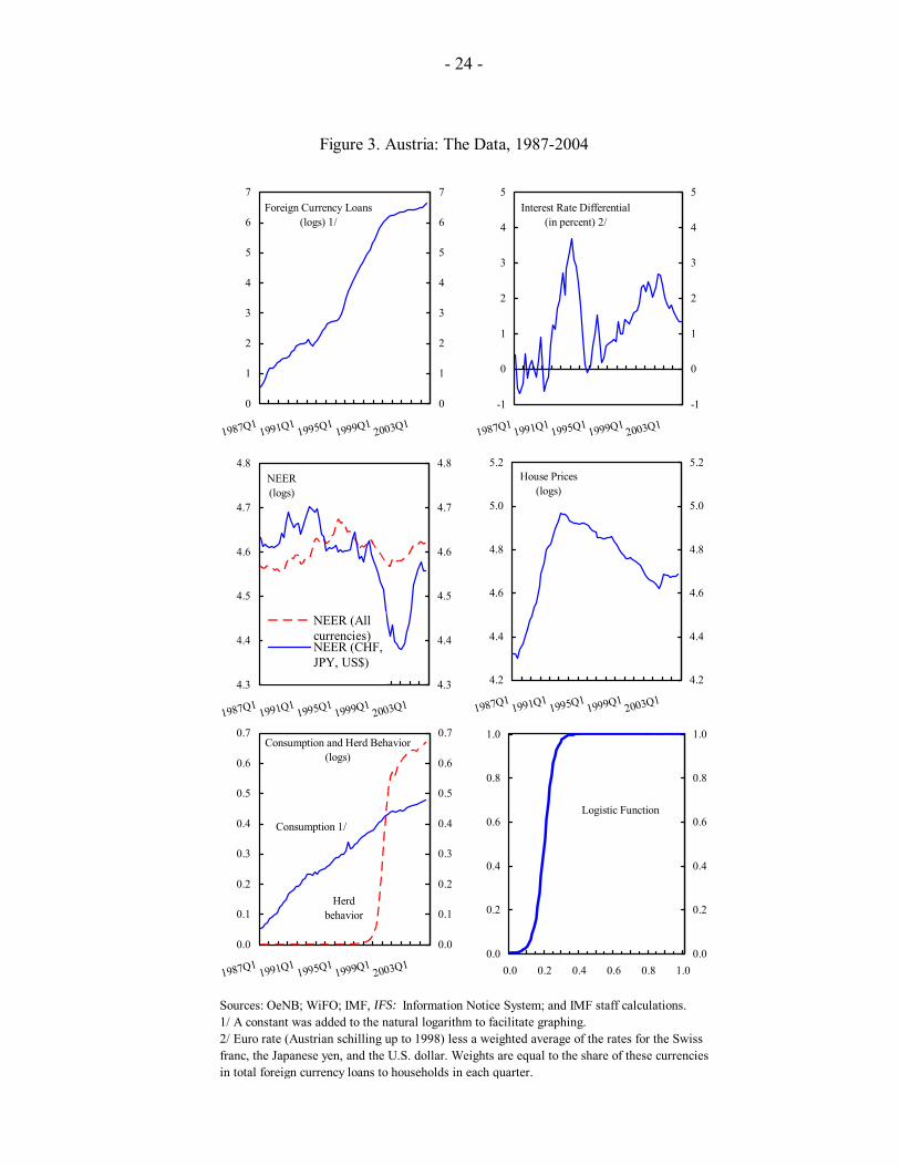
Approved by the European Department
June 29, 2005
Contents Page
I. What Explains the Surge of Foreign Currency Loans to Austrian Households?......... 3 A. Introduction...................................................................................................... 3 B. Issues Related to Foreign Currency Loans to Households .............................. 6 C. The Theoretical Model and the Data ............................................................. 10 D. Estimation of the Long-Run Demand for Loans in Foreign Currency .......... 13 E. A Dynamic Model of Loans in Foreign Currency ......................................... 17 F. Summary of Results ....................................................................................... 19 G. Concluding Remarks...................................................................................... 20 Appendix: A Model of Foreign Currency Loans to Austrian Households ................ 29 References.................................................................................................................. 36 II. Austrian Economic Growth and the Linkages to Germany and Central and Eastern Europe .................................................................................... 38 A. Introduction.................................................................................................... 38 B. The Austrian-German Connection................................................................. 38 C. Austria’s Integration with the CEECs ........................................................... 40 D. Gravity Model Application............................................................................ 47 E. Conclusion ..................................................................................................... 50 Appendix: Definitions of Variables Used in the Cross-Section Regression ............. 52 References.................................................................................................................. 53 Boxes I-1. Summary of the Main Results...................................................................................... 6 I-2. Features of Foreign Currency Loans ........................................................................... 7 I-3. Risks Associated with Loans in Foreign Currency...................................................... 9 I-4. Herd Behavior............................................................................................................ 12 I-5. Estimation Results for 1987–95................................................................................. 14
- 2 -
Figures I-1. Loans in Foreign Currency, 1987–2005 .................................................................... 22 I-2. Interest Rate Differentials and Exchange Rates, 1987–2004 .................................... 23 I-3. The Data, 1987–2004................................................................................................. 24 I-4. Long-Run Equilibrium, and Actual and Fitted Values of Loans in Foreign Currency, 1994–2004.............................................................................................. 25 I-5. Parameter Stability, 1996–2004................................................................................. 26 I-6. Tests for Structural Breaks, 1996–2004 .................................................................... 27 I-7. Real Loans to Households in Foreign Currency, 2003–04........................................ 28 II-1. Austria, Germany, and Euro Zone: Real GDP Growth, 1994-2004 .......................... 39 II-2. Austria’s Trade Intensity with Germany, 1992-2004 ................................................ 41 II-3. Austria and Germany: Output Comovement, 1993-2004 .......................................... 41 II-4. Austria’s Trade Intensity with CEECs, 1992-2004 ................................................... 43 II-5. Austrian FDI in CEECs, 1995-2003 .......................................................................... 44 II-6a. Austria and Germany: Observed vs. Predicted Trade, 1970-97 ................................ 51 II-6b. Austria and Germany: Observed vs. Predicted Trade, 1998-2003 ............................ 51 II-7a. Austria and Hungary: Observed vs. Predicted Trade, 1970-97 ................................. 51 II-7b. Austria and Hungary: Observed vs. Predicted Trade, 1998-2003 ............................. 51 Tables II-1. Distribution of EU-15 Trade (Exports plus Imports) with the Czech Republic, Hungary, and Poland (CHP) combined, 2004 ........................................................ 42 II-2. Results for the Cross-Section Regression.................................................................. 49 Appendix Tables I-1. ADF Statistics Testing for a Unit Root...................................................................... 30 I-2. Johansen Test of Existence of Long-Run Relationships, and Feedback Coefficients, 1987:Q1–1995:Q4............................................................. 31 I-3. Johansen Test of Existence of Long-Run Relationships, and Feedback Coefficients, 1994:Q1–2004:Q3............................................................. 33
- 3 -
I. WHAT EXPLAINS THE SURGE OF FOREIGN CURRENCY LOANS TO AUSTRIAN HOUSEHOLDS?1
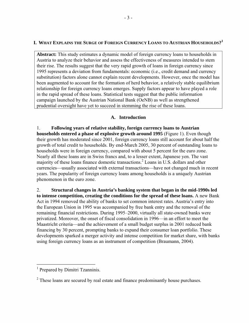
Abstract: This study estimates a dynamic model of foreign currency loans to households in Austria to analyze their behavior and assess the effectiveness of measures intended to stem their rise. The results suggest that the very rapid growth of loans in foreign currency since 1995 represents a deviation from fundamentals: economic (i.e., credit demand and currency substitution) factors alone cannot explain recent developments. However, once the model has been augmented to account for the formation of herd behavior, a relatively stable equilibrium relationship for foreign currency loans emerges. Supply factors appear to have played a role in the rapid spread of these loans. Statistical tests suggest that the public information campaign launched by the Austrian National Bank (OeNB) as well as strengthened prudential oversight have yet to succeed in stemming the rise of these loans.
A. Introduction
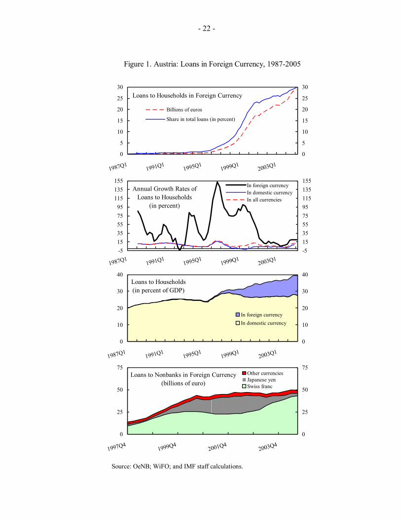
1. Following years of relative stability, foreign currency loans to Austrian households entered a phase of explosive growth around 1995 (Figure 1). Even though their growth has moderated since 2001, foreign currency loans still account for about half the growth of total credit to households. By end-March 2005, 30 percent of outstanding loans to households were in foreign currency, compared with about 5 percent for the euro zone. Nearly all these loans are in Swiss francs and, to a lesser extent, Japanese yen. The vast majority of these loans finance domestic transactions.2 Loans in U.S. dollars and other currencies—usually associated with external transactions—have not changed much in recent years. The popularity of foreign currency loans among households is a uniquely Austrian phenomenon in the euro zone.
2. Structural changes in Austria’s banking system that began in the mid-1990s led to intense competition, creating the conditions for the spread of these loans. A new Bank Act in 1994 removed the ability of banks to set common interest rates. Austria’s entry into the European Union in 1995 was accompanied by free bank entry and the removal of the remaining financial restrictions. During 1995–2000, virtually all state-owned banks were privatized. Moreover, the onset of fiscal consolidation in 1996—in an effort to meet the Maastricht criteria—and the achievement of a small budget surplus in 2001 reduced bank financing by 30 percent, prompting banks to expand their consumer loan portfolio. These developments sparked a merger activity and intense competition for market share, with banks using foreign currency loans as an instrument of competition (Braumann, 2004).
1 Prepared by Dimitri Tzanninis.
2 These loans are secured by real estate and finance predominantly house purchases.
- 4 -
3. The boom in these loans appears to be reflecting currency substitution rather than a lending boom. Growth of credit to households (in all currencies) has been relatively subdued (second panel of Figure 1), suggesting that a considerable part of the growth of foreign currency loans has been the result of refinancing. Indeed, because of refinancing of previous schilling or euro loans, the contribution of foreign currency loans to the annual growth of total loans to households approached or exceeded 100 percent in six consecutive quarters beginning in late 1998.3 The spread of this phenomenon has puzzled many. Heightened concerns about risks prompted policymakers to strengthen prudential oversight and launch a public information campaign in 2003 (OeNB, 2003).
4. This study addresses the following questions:
• Is this phenomenon reflecting an equilibrium rebalancing of portfolios or the buildup of financial imbalances? Is the stock of loans in foreign currency in Austria currently above the steady state equilibrium? If yes, how smooth is the return to equilibrium expected to be?
• In what respects has Austria been different from other euro zone countries? Can Austria-specific factors be uncovered in a statistical way? Has herd behavior played a role?
• Have banks contributed to this development? What can the statistical evidence tell us about the role of the banks?
• Has the housing market been a driving force? How strong is the interaction between these loans and the house and mortgage markets? Could falling prices in the housing market cause serious balance sheet problems for consumers and banks?
• How large are the measurable risks to the economy stemming from these loans? What could the repercussions of large shocks to interest and exchange rates be?
• Can the impact of recent policy measures designed to arrest the growth of these loans be identified? Aside from addressing risk management of banks, have policy measures been effective in stemming the rise of these loans? What role can policy play in this area in a free market economy with an open capital account?
5. The literature on models of lending in foreign currency in advanced economies is thin. Moreover, to the author’s knowledge, there has been no empirical study on this topic for Austria. The voluminous literature on dollarization and currency substitution provides
3 Waschiczek (2002) provides a comprehensive discussion of foreign currency loans in Austria since 1995, their main features and the principal risks involved, and suggests—but does not model—the possibility of herd behavior.
- 5 -
some insights on the choice of currency by households, but focuses mainly on developing and transition countries and on the asset—rather than the liability—side of household balance sheets.4 A possible explanation for the paucity of research on credit dollarization in advanced economies is that the need for understanding the driving forces of the demand for foreign currency loans becomes pressing only when the growth of these loans has already reached sizeable proportions. By then, herd behavior and bandwagon effects—which weaken the influence of fundamentals—have likely come into play, and the challenge in modeling herd behavior makes it difficult to investigate the demand for these loans. The problem of identifying credit demand and supply may also have contributed to the modeling problems.5
6. This study aims to contribute to the understanding of the reasons behind the boom in foreign currency loans in Austria in the following respects. First, it allows for a deviation of the equilibrium foreign currency loans from economic fundamentals by modeling the formation and development of herd behavior explicitly. Second, by recognizing that standard credit demand and currency substitution factors alone may not be sufficient to explain the boom in these loans, it investigates the role of the housing market in a formal way. Finally, it aims to assess in a statistical way the effectiveness of recent policy measures in this area.
7. This study formulates a model of the long-run equilibrium demand for loans that is enriched with short-term dynamics to describe the behavior of foreign currency loans to Austrian households. To put the problem in perspective, Section B discusses the main issues related to these loans. Section C provides a brief overview of the theoretical foundations of the model, as well as an interpretation of the data. Section D uncovers an equilibrium long-run relationship between loans to households in foreign currency and their fundamental determinants, and in the process evaluates the influence of individual factors on the behavior of these loans over the long run. Section E describes a foreign currency loan equation that captures both short- and long-run dynamics, and performs experiments to assess the impact on these loans of large shocks to the variables in the model. Section F summarizes the results. Finally, Section G contains concluding remarks. Box 1 summarizes the results presented in the following sections.
4 See, for example, on the asset side, Komárek and Melecký (2003) for an application of the currency substitution theory to a transition economy, and, on the liability (i.e., credit) side, Luca and Petrova (2003) for a study of 22 transition economies.
5 Using a model of credit aggregates (in all currencies) for four European countries, including Austria, Kaufmann and Valderrama (2004) find credit in Austria to be mostly demand driven.

- 6 -
Box 1. Summary of the Main Results The model is intuitively appealing and fits the data well. The main results are as follows: • The strong uptrend in foreign currency loans since 1995 represents a significant deviation from
fundamentals: economic (i.e., credit demand and currency substitution) factors alone cannot explain developments since 1995, but once the model has been augmented to account for the formation of herd behavior, a relatively stable long-run relationship for foreign currency loans emerges. These loans currently appear to be significantly above the steady state equilibrium level implied by economic fundamentals, but the return to equilibrium is likely to be slow.
• The principal factor that distinguishes Austria from other euro zone countries seems to be the formation of herd behavior in the demand for foreign currency loans. The results suggest that the perception of exchange rate stability shaped by two decades of hard currency policy may also have played a role, albeit modest: the influence of the exchange rate on foreign currency loans is large in the long run but disappears in the short run.
• Banks’ pricing policies may have been a factor behind developments in foreign currency loans. First, demand for these loans appears to have been met by falling interest rates as banks have likely made an effort to gain market share. Second, the transaction costs involved in refinancing these loans may have contributed to the estimated slow return to equilibrium.
• It appears that housing market developments have not played a significant role.
• The response of foreign currency loans to modest shocks (stemming, for example, from a depreciation of the exchange rate) should be relatively modest and gradual.
• Policy measures addressing the demand and supply of foreign currency loans have not had a statistically significant impact on either the levels or growth rates of these loans.
B. Issues Related to Foreign Currency Loans to Households
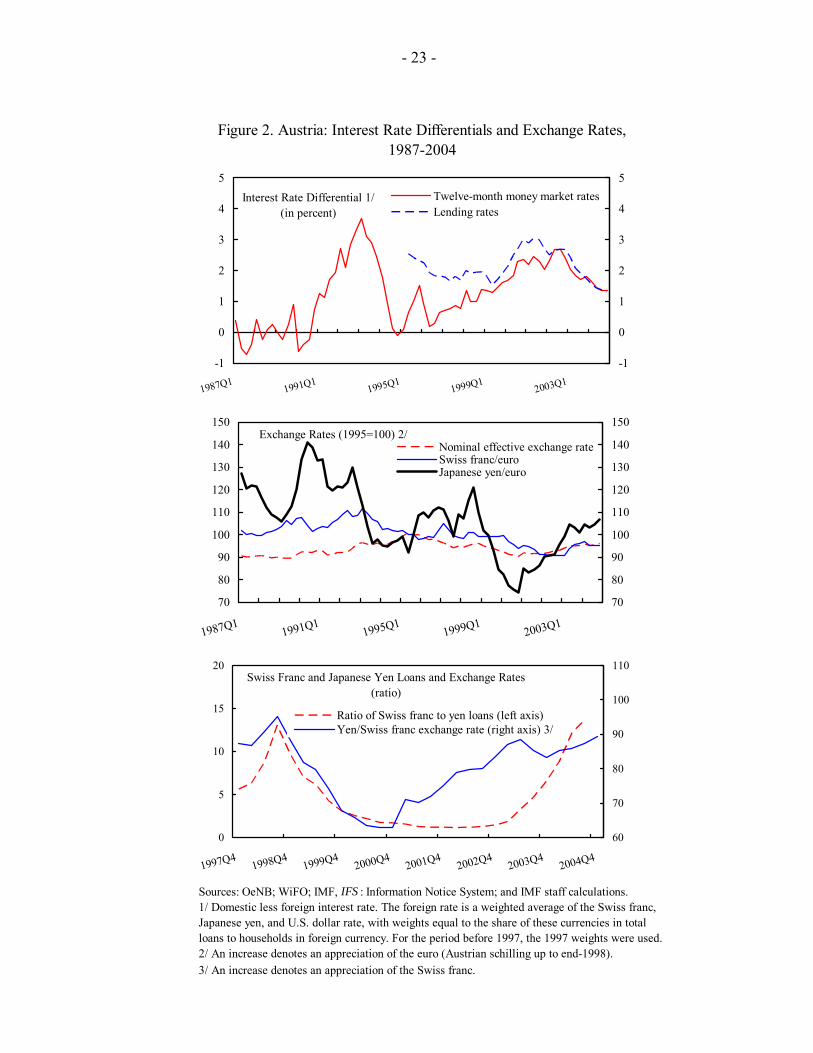
8. The appeal of these loans is mainly in the lower interest rates on the borrowed currencies. Interest rates on these loans are linked to the London interbank offer rate (LIBOR) of the currency of the loan (Box 2). Money market rates for the main currencies of choice have been lower than those for the domestic currency virtually throughout the past 20 years (Figure 2). Despite the appreciation of the Swiss franc and Japanese yen over the same period, it appears that borrowers have been attracted by the lower interest payments and count on a stable exchange rate. Even though the degree of substitution between foreign currency and euro loans does not differ from that between loans in different foreign currencies, exchange rate movements have led to switches to other foreign currencies. The appreciation of the Japanese yen between late 1998 and late 2000 prompted a switch—albeit with a considerable lag—away from the yen to the more stable Swiss franc (bottom panel of Figure 2).
- 7 -
Box 2. Features of Foreign Currency Loans A typical foreign currency loan to an Austrian household • is used predominantly for purchasing a house and has a size of about EUR 100,000;
• is secured by real estate collateral;
• has a relatively low loan-to-value ratio;
• has a maturity of up to 25 years;
• has an adjustable interest rate linked to the LIBOR rate of the currency of the loan and is repriced every three to six months;
• is a balloon loan (involving monthly payments of interest only, with full principal paid at maturity);
• has a narrower interest margin and carries higher fees than a comparable euro loan;
• offers the option of switching currencies—typically at repricing dates—for a 1-2 percent conversion fee;
• has forced conversion clauses, allowing conversion into a euro loan without the borrower’s consent; and
• requires the establishment of a repayment vehicle (usually a life insurance contract or a mutual fund) through which monthly payments are made and which is to be used to repay the principal at maturity.
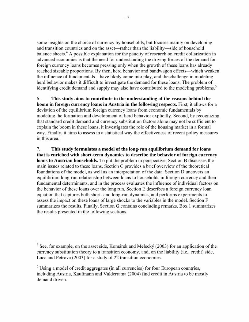
Sources: Financial Market Authority; OeNB; IMF (2004); and Waschiczek (2002). 9. With common interest and exchange rates in the other euro zone countries, why have these loans taken off only in Austria? The practice of borrowing in foreign currency (mainly Swiss francs) began in the western part of the country, where tens of thousands of Austrians commute to work in Switzerland and Liechtenstein. This partly explains why the share of these loans was higher in Austria, even during the 1980s. Word of mouth and aggressive promotion by financial advisors helped spread the popularity of these loans to the rest of the country. By the mid-1990s, newspaper ads placed by banks began to appear, fueling public interest (text figure). Another factor facilitating the spread of these loans could be the belief in the stability of the exchange rate deriving from Austria’s hard currency policy (a peg of the schilling to the deutsche mark) since 1980.6 The success of this policy may have created a psychology of an exchange rate immune from risks, notwithstanding the appreciation of the Japanese yen and, to a lesser extent, the Swiss franc since the mid-1980s.
6 Gnan (1994) studies the hard currency policy in Austria since its adoption in 1980.
0
10
20
30
40
50
1987Q11991Q1
1995Q11999Q1
2003Q1
0
10
20
30
40
50Austrian Press Agency News Stories
on Foreign Currency Loans,1987-2004 1/
Source: Factiva's NewsPlus.1/ Number of news reports (in German) by the Austrian Press Agency that included the word "fremdwaehrungskredite" (foreign currency loans). Waschczek (2002) has presented the results of a similar search of news reports.
- 8 -
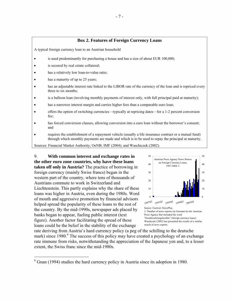
10. At first glance, Austria’s house and mortgage markets do not appear to explain the boom in these loans. The experience of other countries suggests that house prices influence mortgage borrowing (the predominant liability of households) through two channels. First, a rise in house prices typically requires a larger mortgage to acquire a given property. Second, fluctuating house prices affect the capacity of households to borrow through the change in the value of their collateral (mortgage equity withdrawal). This relationship has become stronger since the 1980s, as financial reforms have increased households’ access to mortgage borrowing. However, some mitigating factors appear to be at work in the house and mortgage markets in Austria. The boom in house prices that began in the mid-1980s halted in the first half of the 1990s as the supply of housing increased (text figure). House prices have edged up somewhat recently, but remain well below their long-run average.7 Moreover, Austria’s owner occupation rates are among the highest and outstanding mortgage debt one of the lowest in Europe. This could imply a weak transmission mechanism from the house and mortgage markets to the rest of the economy. However, house prices could still have played a role in helping foreign currency loans take off (a hypothesis that can be tested empirically), even though they do not appear to have played a role in recent years.8
11. Foreign currency loans expose households to a host of risks (Box 3). The experience of other countries—for example, Australia, and, to some extent, the United Kingdom in the 1980s—suggest that severe balance sheet problems, mainly for households, could develop in the event of a large and rapid exchange rate movement, with repercussions felt throughout the economy.9 Concerned about these risks, the OeNB and the Financial Market Authority (FMA) implemented a number of measures: the OeNB launched a public information campaign in mid-2003 and, together with the FMA, intensified prudential oversight and took steps to strengthen banks’ risk management.
7 Ball (2004) reviews the structure of Austria’s house and mortgage markets and discusses recent developments.
8 Hofmann (2001) provides empirical evidence of a relationship between credit and property prices in 16 industrialized countries.
9 Kingston (1995) discusses the economic and legal issues related to the fall of the Australian dollar and the surge of foreign currency liabilities in Australia in the 1980s.
40
70
100
130
1987Q11991Q1
1995Q11999Q1
2003Q1
40
70
100
130
Real house pricesHouse prices to disposable income
House Prices, 1987-2003(1995=100)
Trend in house prices
- 9 -
Box 3. Risks Associated with Loans in Foreign Currency Households Loans in foreign currency expose households to the following risks: • Exchange rate risk, from households’ large, unhedged exposure. The switch away from the Japanese
yen to the more stable Swiss franc has mitigated this risk. Nevertheless, this risk is still not trivial and can be aggravated by the fact that the full principal is not due until maturity, which may be many years away. While, in principle, the repayment vehicle could be used to mitigate this risk, in practice, multicurrency exposure often occurs when households invest in a third currency.
• Interest rate risk from the adjustable-rate loans with frequent repricing dates.
• Additional market risk from the uncertain returns of the investment in repayment vehicles.
• Maturity mismatch risk of assets and liabilities. Household assets (repayment vehicles) offer long-term returns, while liabilities (foreign currency loans) are exposed to short-term rates.
• Double-exposure risk from borrowing in foreign currency and investing in real estate. The assets usually funded by foreign currency loans are real estate, a nontraded good, which tends to underperform when the terms of trade are depressed. With a correlation coefficient between Austria’s nominal effective exchange rate (NEER) and the housing price index for 1987–2003 of 0.72, a household could be hit adversely by the same shock (namely, depreciation of the domestic currency) on both the asset and liability sides of its balance sheet.
• Litigation risk. Forced conversion clauses in loan contracts have their drawbacks: in the event of a depreciation and subsequent strengthening of the euro, the households would have locked-in their losses while missing the opportunity to get loans with the potential for capital gains. This could create frictions with the banks, undermine confidence, and lead to litigation.
Banks Even though banks have limits on open foreign exchange positions, are largely hedged, and apply conservative loan-to-value ratios, they are exposed to indirect risk. Risks to the banks include:
• Credit risk from the default of households, including from borrowers’ exposure to market risk.
• Reputation and litigation risk from large losses suffered by clients and from the liquidation of their collateral.
• Concentration risk from the homogeneity of collateral and the possible bank losses resulting from having to sell large amounts of real estate in small markets. Low loan-to-value ratios in Austria mitigate this risk but could still be considerable if many households default in the same market.
Government There is a political risk that households might hold policymakers responsible for their having suffered large losses, arguing that they were not warned or protected adequately.
- 10 -
C. The Theoretical Model and the Data
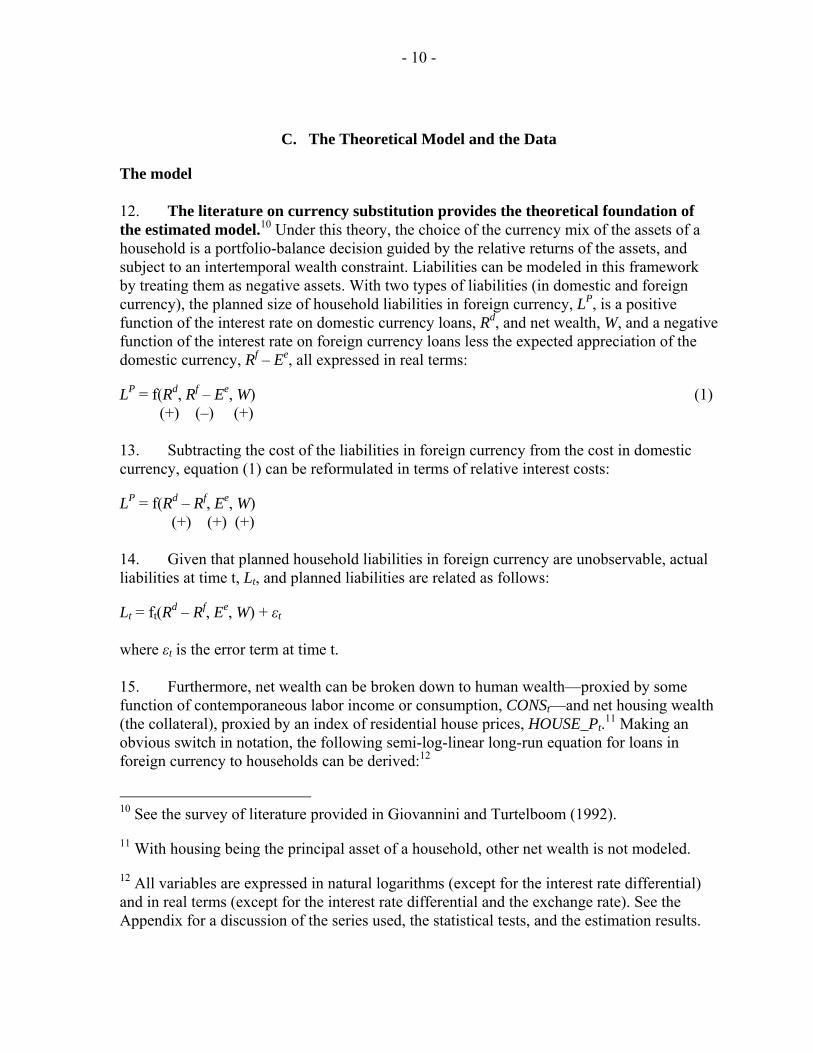
The model 12. The literature on currency substitution provides the theoretical foundation of the estimated model.10 Under this theory, the choice of the currency mix of the assets of a household is a portfolio-balance decision guided by the relative returns of the assets, and subject to an intertemporal wealth constraint. Liabilities can be modeled in this framework by treating them as negative assets. With two types of liabilities (in domestic and foreign currency), the planned size of household liabilities in foreign currency, LP, is a positive function of the interest rate on domestic currency loans, Rd, and net wealth, W, and a negative function of the interest rate on foreign currency loans less the expected appreciation of the domestic currency, Rf – Ee, all expressed in real terms:
LP = f(Rd, Rf – Ee, W) (1) (+) (–) (+) 13. Subtracting the cost of the liabilities in foreign currency from the cost in domestic currency, equation (1) can be reformulated in terms of relative interest costs:
LP = f(Rd – Rf, Ee, W) (+) (+) (+) 14. Given that planned household liabilities in foreign currency are unobservable, actual liabilities at time t, Lt, and planned liabilities are related as follows:
Lt = ft(Rd – Rf, Ee, W) + εt where εt is the error term at time t. 15. Furthermore, net wealth can be broken down to human wealth—proxied by some function of contemporaneous labor income or consumption, CONSt—and net housing wealth (the collateral), proxied by an index of residential house prices, HOUSE_Pt.11 Making an obvious switch in notation, the following semi-log-linear long-run equation for loans in foreign currency to households can be derived:12
10 See the survey of literature provided in Giovannini and Turtelboom (1992).
11 With housing being the principal asset of a household, other net wealth is not modeled.
12 All variables are expressed in natural logarithms (except for the interest rate differential) and in real terms (except for the interest rate differential and the exchange rate). See the Appendix for a discussion of the series used, the statistical tests, and the estimation results.
- 11 -
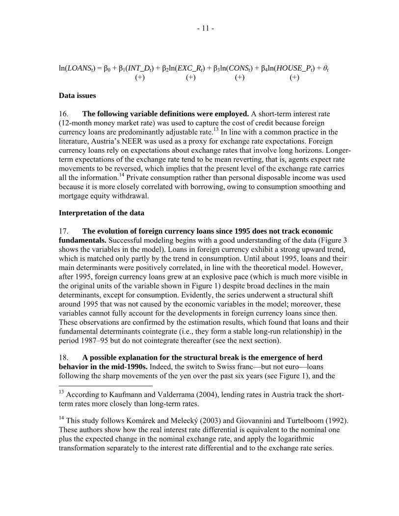
ln(LOANSt) = β0 + β1(INT_Dt) + β2ln(EXC_Rt) + β3ln(CONSt) + β4ln(HOUSE_Pt) + θt (+) (+) (+) (+)
Data issues 16. The following variable definitions were employed. A short-term interest rate (12-month money market rate) was used to capture the cost of credit because foreign currency loans are predominantly adjustable rate.13 In line with a common practice in the literature, Austria’s NEER was used as a proxy for exchange rate expectations. Foreign currency loans rely on expectations about exchange rates that involve long horizons. Longer-term expectations of the exchange rate tend to be mean reverting, that is, agents expect rate movements to be reversed, which implies that the present level of the exchange rate carries all the information.14 Private consumption rather than personal disposable income was used because it is more closely correlated with borrowing, owing to consumption smoothing and mortgage equity withdrawal.
Interpretation of the data 17. The evolution of foreign currency loans since 1995 does not track economic fundamentals. Successful modeling begins with a good understanding of the data (Figure 3 shows the variables in the model). Loans in foreign currency exhibit a strong upward trend, which is matched only partly by the trend in consumption. Until about 1995, loans and their main determinants were positively correlated, in line with the theoretical model. However, after 1995, foreign currency loans grew at an explosive pace (which is much more visible in the original units of the variable shown in Figure 1) despite broad declines in the main determinants, except for consumption. Evidently, the series underwent a structural shift around 1995 that was not caused by the economic variables in the model; moreover, these variables cannot fully account for the developments in foreign currency loans since then. These observations are confirmed by the estimation results, which found that loans and their fundamental determinants cointegrate (i.e., they form a stable long-run relationship) in the period 1987–95 but do not cointegrate thereafter (see the next section).
18. A possible explanation for the structural break is the emergence of herd behavior in the mid-1990s. Indeed, the switch to Swiss franc—but not euro—loans following the sharp movements of the yen over the past six years (see Figure 1), and the 13 According to Kaufmann and Valderrama (2004), lending rates in Austria track the short-term rates more closely than long-term rates.
14 This study follows Komárek and Melecký (2003) and Giovannini and Turtelboom (1992). These authors show how the real interest rate differential is equivalent to the nominal one plus the expected change in the nominal exchange rate, and apply the logarithmic transformation separately to the interest rate differential and to the exchange rate series.
- 12 -
associated capital losses incurred by a number of borrowers suggest that entrenched herd behavior might have been at play (Box 4). While it is unclear what exactly triggered the herd behavior, the factors mentioned in paragraph 9 might have played a role. Consequently, a variable proxying herd behavior was added to the model to help explain developments since 1995.
Box 4. Herd Behavior Herd behavior occurs when people do what others do rather than rely on their own (incomplete) information, which might be suggesting something different (Banerjee, 1992). The suppression of private information could lead to “information cascades” when decisions are made sequentially and a large enough number of people choose identical actions. In such settings, the decisions of a critical few people early on are enough to tilt group behavior toward a certain direction. Mimicking the behavior of others might be rational because of uncertainty about one’s own information as well as the need to economize on information-gathering costs. Rational herd behavior is the subject of a recent strand of behavioral finance (see Montier, 2002, for an introduction). Herd behavior can arise in a variety of environments, including in financial markets. However, it is difficult to disentangle empirically the effects of macroeconomic or other fundamental determinants from those caused by herd behavior. Herd behavior often results in volatility because it is susceptible to abrupt shifts or reversals, and thus has the potential to destabilize markets. Empirical studies have shown that the dynamics of herd behavior often resemble an S curve: initially only a few adopt a certain behavior, but, past a certain critical mass, a take-off state takes hold where a rapidly growing number of people adopt this behavior. Toward the end of this process, a moderation of the dynamics takes place as the potential pool of adoptees is exhausted. These dynamics are often modeled using a logistic growth model, because of the ability of the logistic function to capture the dynamics of herd behavior: see Tsoularis (2001) for a discussion of logistic growth models in the context of several applications; and Yoshifuji and Demizu (1998), Levi-Faur (2002), and Maggioni (2004) for formal models of herd behavior in various markets, using variations of the logistic function.
19. Herd behavior was modeled as a logistic function. The logistic function 1/(1+α/eβx) was fitted with the share of foreign currency loans in total loans to households (argument x). It was parameterized so that it exhibits the following properties: the function takes off at just under x = 5 percent (roughly the share around 1995 when these loans took off—see Figure 1) and slows down around x = 30 percent (just above the present share, which has been accompanied by moderating growth).15 Moreover, the function was scaled up by a constant (one) so that its natural logarithm takes only positive values. The bottom panels of Figure 3 show the resulting proxy variable for herd behavior and the underlying logistic function.
15 Parameterization of the logistic function based on the properties of the data is not uncommon in the literature of herd behavior (see, for example, Alevy et al, 2003, and Drehmann et al, 2003). Nevertheless, the results of this study were largely invariant to different parameterizations.
- 13 -
20. The logistic function employed here has a number of appealing properties that track closely the evolution of foreign currency loans in Austria. First, it is an exponentially increasing function of the share of foreign currency loans in total loans: the larger the number of households who have a foreign currency loan, the faster the spread of the word of mouth. Second, it requires a critical mass to take off: unlike other euro zone countries, Austria was near this critical mass because of the popularity of foreign currency loans in the western part of the country, and a small perturbation was sufficient to set the herd process in motion. Third, it accelerates as the herd behavior gathers momentum, which describes loan developments since 1995. Finally, its pace of expansion eventually slows, as most of those who wanted to jump on the bandwagon have already done so, as currently appears to be the case (see Figure 1).
21. Tests for the nonstationarity of the variables in the model suggest that loans in foreign currency and the variable for herd behavior could be I(2) processes, that is, double differencing is needed to make the series stationary (see the Appendix). This requires that the search for a stationary linear combination of all variables (called the cointegrating vector) be done using Johansen’s I(2) cointegration analysis.16
22. Cointegration analysis of I(2) processes is complicated, and the long-run equilibrium may involve not only the levels, but also the differences of the I(2) variables.17 This involves: (i) searching for a linear combination of the two I(2) variables (namely, loans in foreign currency and the proxy for herd behavior) that is an I(1) process; and (ii) using this combination to transform the two variables into a single one, and focusing on the I(1) system. This has the added appeal that, if foreign currency loans and the variable for herd behavior cointegrate (and thus can be transformed to a single variable), then the influence of true “economic” factors can be separated from that of herd behavior in the demand for loans in foreign currency. This study follows this modeling approach, and the following section presents the model for the transformed variable. Inference from the transformed system involves no loss of information, provided that the two I(2) variables share one common I(2) trend that enters the cointegrating relation with the coefficients found in the unrestricted model.
D. Estimation of the Long-Run Demand for Loans in Foreign Currency
23. The search for a stable and meaningful long-run relationship between foreign currency loans and their determinants was unsuccessful for the full sample (1987:Q1–2004:Q3). Because of the structural break around 1995, the estimation could not establish a long-run cointegrating relationship (interpreted as steady state equilibrium) between real 16 See Johansen (1992) for an application of the I(2) analysis to Australian and U.S. data.
17 Fiess and MacDonald (2001) explain the steps involved in estimating I(2) models with an application to Danish data.
- 14 -
loans to households in foreign currency and the following: (i) their fundamental determinants (the nominal interest rate differential, the nominal exchange rate, real consumption, and real house prices); (ii) the proxy for herd behavior; and (iii) a dummy variable capturing the effects of the policy measures since mid-2003 mentioned in paragraph 11. The search was unsuccessful even after house prices and the dummy were dropped from the model.
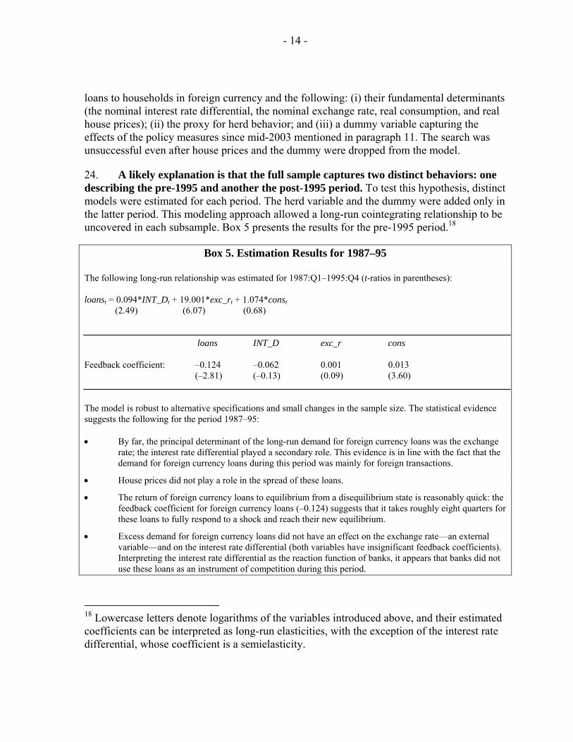
24. A likely explanation is that the full sample captures two distinct behaviors: one describing the pre-1995 and another the post-1995 period. To test this hypothesis, distinct models were estimated for each period. The herd variable and the dummy were added only in the latter period. This modeling approach allowed a long-run cointegrating relationship to be uncovered in each subsample. Box 5 presents the results for the pre-1995 period.18
Box 5. Estimation Results for 1987–95
The following long-run relationship was estimated for 1987:Q1–1995:Q4 (t-ratios in parentheses): loanst = 0.094*INT_Dt + 19.001*exc_rt + 1.074*const (2.49) (6.07) (0.68) loans INT_D exc_r cons Feedback coefficient: –0.124 –0.062 0.001 0.013 (–2.81) (–0.13) (0.09) (3.60) The model is robust to alternative specifications and small changes in the sample size. The statistical evidence suggests the following for the period 1987–95: • By far, the principal determinant of the long-run demand for foreign currency loans was the exchange
rate; the interest rate differential played a secondary role. This evidence is in line with the fact that the demand for foreign currency loans during this period was mainly for foreign transactions.
• House prices did not play a role in the spread of these loans.
• The return of foreign currency loans to equilibrium from a disequilibrium state is reasonably quick: the feedback coefficient for foreign currency loans (–0.124) suggests that it takes roughly eight quarters for these loans to fully respond to a shock and reach their new equilibrium.
• Excess demand for foreign currency loans did not have an effect on the exchange rate—an external variable—and on the interest rate differential (both variables have insignificant feedback coefficients). Interpreting the interest rate differential as the reaction function of banks, it appears that banks did not use these loans as an instrument of competition during this period.
18 Lowercase letters denote logarithms of the variables introduced above, and their estimated coefficients can be interpreted as long-run elasticities, with the exception of the interest rate differential, whose coefficient is a semielasticity.
- 15 -
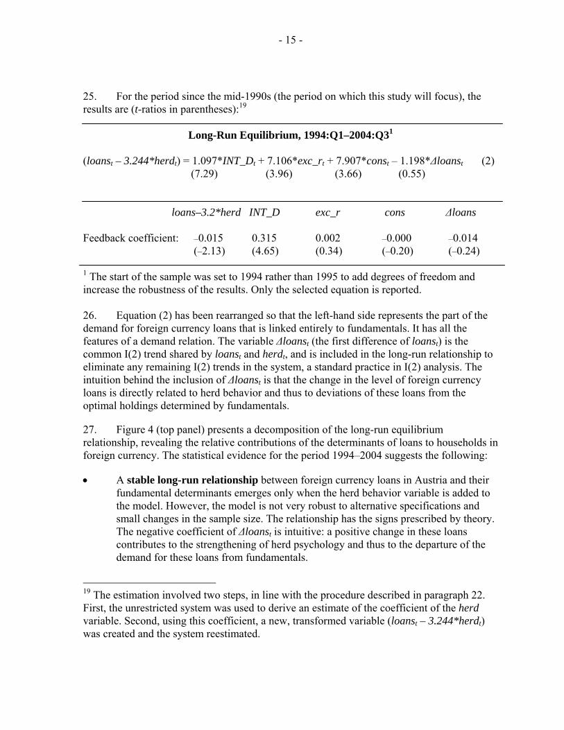
25. For the period since the mid-1990s (the period on which this study will focus), the results are (t-ratios in parentheses):19
Long-Run Equilibrium, 1994:Q1–2004:Q31
(loanst – 3.244*herdt) = 1.097*INT_Dt + 7.106*exc_rt + 7.907*const – 1.198*∆loanst (2) (7.29) (3.96) (3.66) (0.55) loans–3.2*herd INT_D exc_r cons ∆loans Feedback coefficient: –0.015 0.315 0.002 –0.000 –0.014 (–2.13) (4.65) (0.34) (–0.20) (–0.24) 1 The start of the sample was set to 1994 rather than 1995 to add degrees of freedom and increase the robustness of the results. Only the selected equation is reported. 26. Equation (2) has been rearranged so that the left-hand side represents the part of the demand for foreign currency loans that is linked entirely to fundamentals. It has all the features of a demand relation. The variable ∆loanst (the first difference of loanst) is the common I(2) trend shared by loanst and herdt, and is included in the long-run relationship to eliminate any remaining I(2) trends in the system, a standard practice in I(2) analysis. The intuition behind the inclusion of ∆loanst is that the change in the level of foreign currency loans is directly related to herd behavior and thus to deviations of these loans from the optimal holdings determined by fundamentals.
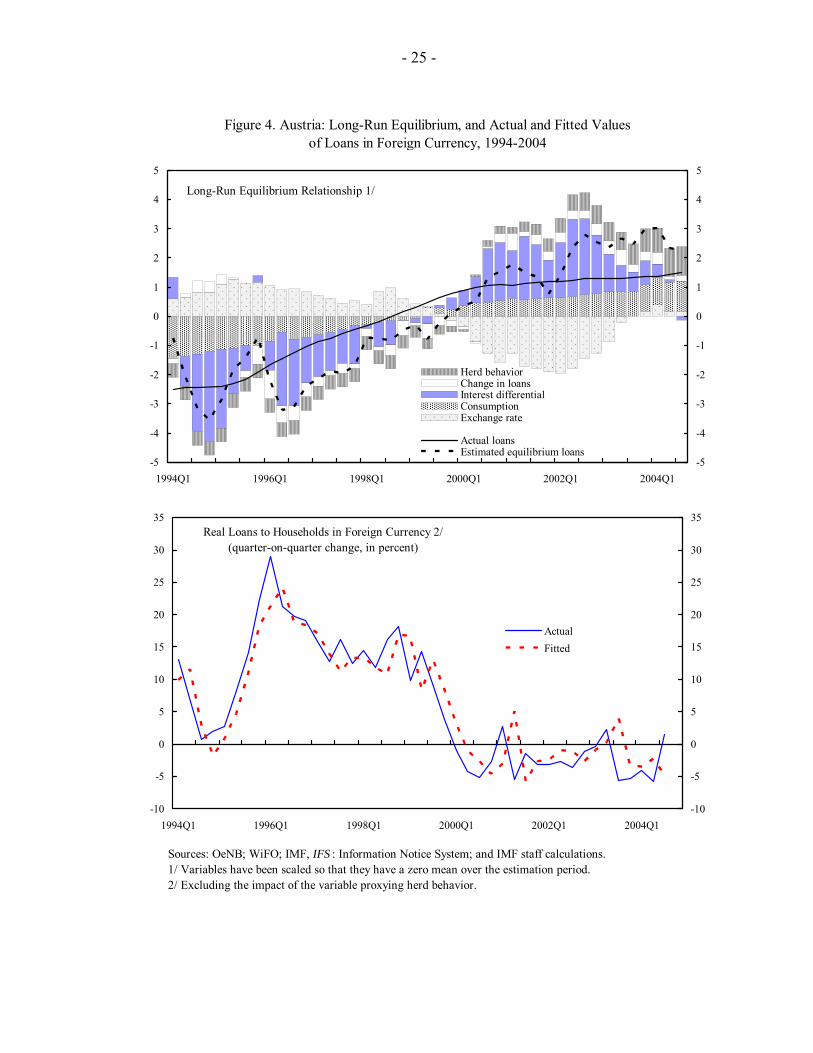
27. Figure 4 (top panel) presents a decomposition of the long-run equilibrium relationship, revealing the relative contributions of the determinants of loans to households in foreign currency. The statistical evidence for the period 1994–2004 suggests the following:
• A stable long-run relationship between foreign currency loans in Austria and their fundamental determinants emerges only when the herd behavior variable is added to the model. However, the model is not very robust to alternative specifications and small changes in the sample size. The relationship has the signs prescribed by theory. The negative coefficient of ∆loanst is intuitive: a positive change in these loans contributes to the strengthening of herd psychology and thus to the departure of the demand for these loans from fundamentals.
19 The estimation involved two steps, in line with the procedure described in paragraph 22. First, the unrestricted system was used to derive an estimate of the coefficient of the herd variable. Second, using this coefficient, a new, transformed variable (loanst – 3.244*herdt) was created and the system reestimated.
- 16 -
• The estimation could not establish a link between foreign currency loans and more recent house price developments.20
• Recent policy measures do not appear to have influenced the long-run demand for foreign currency loans. The dummy variable proxying these measures either did not cointegrate with the other variables or was not statistically significant.
• Loans in foreign currency appear to be highly sensitive over the long run to changes in the exchange rate and consumption, with long-run elasticities over 7. The large coefficients for these two variables most likely capture financial liberalization and the ongoing internationalization of the Austrian economy, as well as deviations from fundamentals not fully captured by the variable for herd behavior.21
• The large, positive, and highly significant feedback coefficient for INT_Dt, which captures the response of the interest rate differential to excess demand for foreign currency loans, lends support to the hypothesis that banks have competed for market share since the mid-1990s by lowering interest rates on these loans, while probably recouping the lost revenue through higher fees on these loans.22 This positive response feeds back into the demand for loans, slowing its return to equilibrium.
• Foreign currency loans adjust to equilibrium from a disequilibrium state very slowly (the feedback coefficient of the transformed variable for loans is –0.015). This is consistent with households’ reluctance to switch currencies in response to a shock, partly because of the transaction fees charged by banks.
• Much of the strength of loans in foreign currency in recent years seems to be due to herd behavior, with the perceived lower cost of these loans (interest rate differential adjusted for exchange rate movements) still playing an important, though diminishing, role (see Figure 4, top panel). The influence of herd behavior appears to have increased in 2004, largely offsetting the effect from the decline in the interest rate differential and accounting for about half the current level of these loans.
20 The absence of an empirical link—though consistent with currency substitution rather than higher demand for mortgages and houses—does not allow the use of the model for the study of counterfactual scenarios involving shocks to house prices and their impact on consumption.
21 The high elasticities—especially that for consumption—are not very appealing from an economic perspective, but the other features of the estimated model offer useful insights.
22 Waschiczek (2002) argues that increased bank competition narrowed the spreads on foreign currency loans.
- 17 -
28. The next step in the estimation of the model is to combine the long-run relationship with short-run influences in a single dynamic equation of foreign currency loans.
E. A Dynamic Model of Loans in Foreign Currency
Error-correction model 29. Deviations of foreign currency loans from their long-run equilibrium levels do not always reflect disequilibria; they also reflect temporary factors and adjustment lags. To capture the short-run dynamics, foreign currency loans were modeled in an error-correction representation, using—in addition to the variables mentioned above—a dummy variable attempting to capture the effect of recent policy measures on the growth rate of these loans.
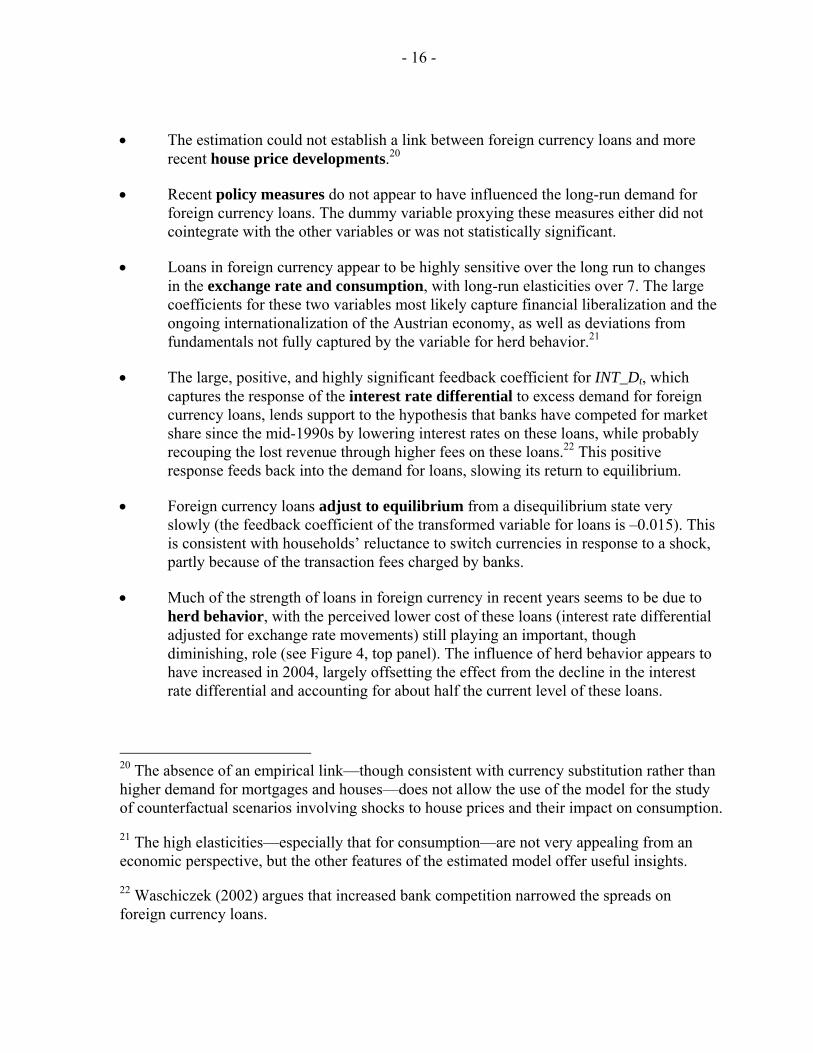
30. Starting from a general specification that includes several lags and variables and reducing it to a parsimonious representation with the aid of appropriate tests, the estimation yielded the following error-correction model of foreign currency loans for 1994:Q1–2004:Q3:23
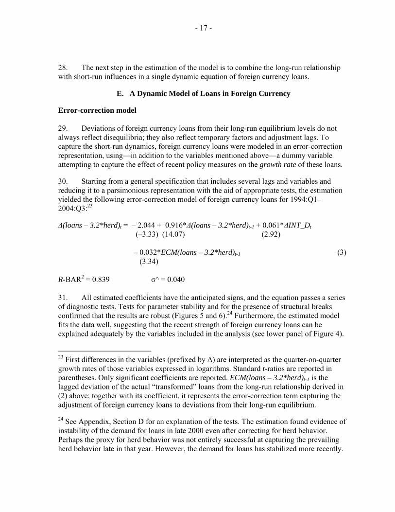
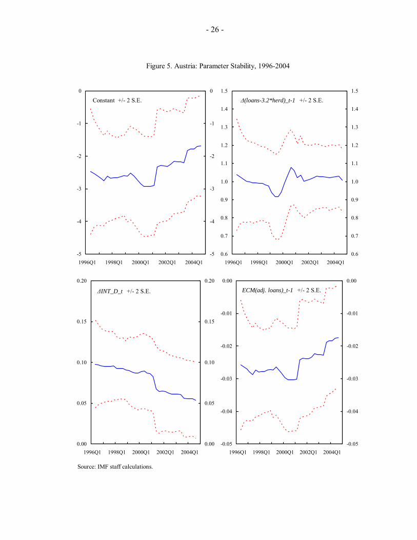
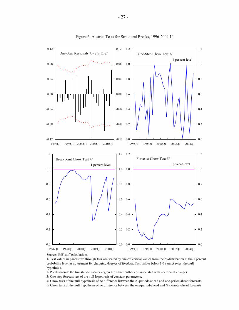
∆(loans – 3.2*herd)t = – 2.044 + 0.916*∆(loans – 3.2*herd)t-1 + 0.061*∆INT_Dt (–3.33) (14.07) (2.92) – 0.032*ECM(loans – 3.2*herd)t-1 (3) (3.34) R-BAR2 = 0.839 σ^ = 0.040 31. All estimated coefficients have the anticipated signs, and the equation passes a series of diagnostic tests. Tests for parameter stability and for the presence of structural breaks confirmed that the results are robust (Figures 5 and 6).24 Furthermore, the estimated model fits the data well, suggesting that the recent strength of foreign currency loans can be explained adequately by the variables included in the analysis (see lower panel of Figure 4).
23 First differences in the variables (prefixed by ∆) are interpreted as the quarter-on-quarter growth rates of those variables expressed in logarithms. Standard t-ratios are reported in parentheses. Only significant coefficients are reported. ECM(loans – 3.2*herd)t-1 is the lagged deviation of the actual “transformed” loans from the long-run relationship derived in (2) above; together with its coefficient, it represents the error-correction term capturing the adjustment of foreign currency loans to deviations from their long-run equilibrium.
24 See Appendix, Section D for an explanation of the tests. The estimation found evidence of instability of the demand for loans in late 2000 even after correcting for herd behavior. Perhaps the proxy for herd behavior was not entirely successful at capturing the prevailing herd behavior late in that year. However, the demand for loans has stabilized more recently.
- 18 -
32. The quarter-on-quarter growth rate of foreign currency loans to households is highly autoregressive (as evidenced by the large short-run coefficient of ∆(loans – 3.2*herd)t-1 in (3), signaling considerable momentum in the growth rates of these loans and providing evidence of the influence of herd behavior, even in the short run. Among economic variables, only the interest rate differential appears to influence short-term fluctuations of the demand for loans in foreign currency. However, rolling regression estimates suggest that the relation between the growth of foreign currency loans and changes in the interest rate differential has weakened over the past several years (see bottom-left panel of Figure 5), suggesting that cost savings are becoming less of a driving force behind the growth of these loans.
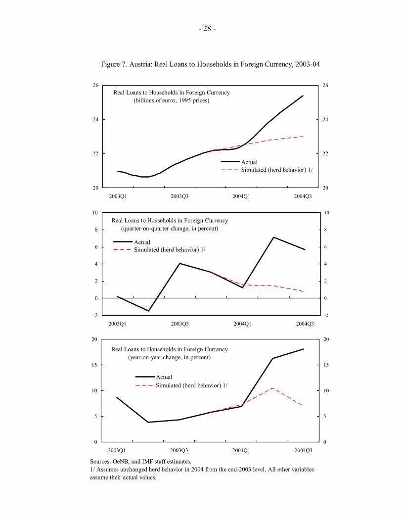
Dynamic simulations 33. How much did the strength of loan growth in 2004 depend on the contribution of herd behavior? A dynamic simulation of the error-correction model in (3)—which involved holding herd behavior constant at its end-2003 level during 2004—indicates that the year-on-year growth of foreign currency loans would have slowed to around 7 percent (Figure 7). This simulation confirms the result from decomposing the cointegrating relationship that much of the recent strength of these loans derives from the steady influence of herd behavior (see Figure 4). It also provides a lower bound estimate of the impact of the policy measures outlined in paragraph 11 on the prospective developments in foreign currency loans during 2004, should the measures had been successful in mitigating herd behavior.
34. Dynamic simulations were also performed to test the response of foreign currency loans to large, counterfactual shocks to their economic determinants. Each determinant was subjected to a structured shock, and the depth and duration of the impact on foreign currency loans were observed.25 The experiments suggest that foreign currency loans have become quite resilient to relatively large adverse shocks to their economic determinants, though the extent and duration of the impact on loan growth do vary among the controlled variables.
35. The counterfactual simulations should be interpreted with caution because they are based on partial analysis. With given paths for the explanatory variables, the simulations preclude feedbacks between variables. For instance, it is likely that a decline in the exchange rate of a larger magnitude than that assumed in the experiment would be accompanied by other developments (such as erosion of confidence) that could have a larger
25 Each explanatory variable was subjected to a negative shock in 2002:Q4, equivalent to two standard deviations below the average year-on-year historical rates of change. The variable was interpolated linearly between 2001:Q4 (the last actual value used) and 2002:Q4 (when the full force of the shock was felt), and remained unchanged thereafter. All other explanatory variables assumed their actual values. The starting point of the simulation was selected to allow the dynamics to play out fully by the end of the period (2004:Q3).
- 19 -
impact on foreign currency loans (and through those to economic activity variables, such as consumption) than the one suggested by the experiments.
F. Summary of Results
36. The main results of the model can be summarized as follows:
• The demand for foreign currency loans in Austria began to exhibit a departure from fundamentals around 1995. A variable capturing herd behavior appears to be successful in isolating the effects of the fundamental economic variables in household demand for foreign currency loans. These loans currently appear to be significantly above the steady state equilibrium level implied by economic fundamentals, but the return to equilibrium is likely to be slow.
The exchange rate plays an important role in the long run but does not appear to have a statistically significant influence on foreign currency loans in the short run. This finding is consistent with the observed lag in switching to the Swiss franc following the protracted rise of the Japanese yen. It suggests that exchange rate movements need to be persistent in order to be taken into account and overcome the psychology of a stable exchange rate.
The interest rate differential seems to play an important—albeit diminishing—role in explaining the short-run dynamics of foreign currency loans: the estimated coefficient in the error-correction model implies that, if the differential were to rise by 10 basis points, the immediate impact on quarter-on-quarter loan growth would be an increase of roughly 0.6 percentage point.26
• The principal factor that distinguishes Austria from other euro zone countries seems to be the formation of herd behavior in the demand for foreign currency loans. The roots of this behavior can be traced to the western part of the country. But unlike other euro zone countries that may have seen pockets of household borrowing in foreign currency in some regions, Austria was near the critical mass required for the onset of herd behavior because of the large popularity of these loans in the western part of the country even since the 1980s. It is likely that some Austria-specific factors, including structural changes in the Austrian banking system, helped trigger the herd behavior.
• Supply factors (notably banks’ pricing policies) appear to have played a role:
26 This result is based on a partial analysis, which does not allow for the impact of a rise in the interest rate differential on the other variables. Moreover, it applies only to small changes.
- 20 -
The reaction of banks to excess demand for foreign currency loans appears to have changed since the mid-1990s. The feedback coefficient for the interest rate differential is statistically equal to zero in the pre-1995 period but large, positive, and highly significant thereafter. This suggests that banks have responded to the growing demand for these loans by lowering interest rates to maintain or gain market share.
Foreign currency loans adjust very slowly to deviations from their long-run equilibrium, pointing once again to a possible reluctance of households to switch currencies in the face of shocks owing to transaction fees.
• It appears that housing market developments have not played a significant role.
• The response of foreign currency loans to modest shocks (stemming, for example, from a depreciation of the exchange rate) should be relatively modest and gradual. Nonetheless, major and protracted declines could have a substantial impact, especially when accompanied by erosion of confidence, and spill over to the rest of the economy. These loans are more responsive to changes in herd behavior.
• Policy measures and the public information campaign have yet to cause a decline in either the level or the growth rate of these loans. Dummy variables in both the long-run relationship and the short-run error-correction equation were statistically insignificant. The observed decline in 2004 in the transformed demand for loans (after adjusting for the influence of herd behavior) is fully accounted for by economic determinants (see top panel of Figure 4).
G. Concluding Remarks
37. The rapid growth of foreign currency loans to Austrian households has raised questions about the forces driving this increase and heightened concerns about risks. This study aimed to uncover both the short- and long-run influences on foreign currency loans and to assess their prospects. The results are generally robust, the estimated model has a dynamic structure and appealing economic interpretation, and performs well in explaining the data.
38. Certain themes emerged consistently throughout various aspects of the empirical investigation. The rapid spread of the popularity of foreign currency loans among households seems to reflect to a significant extent herd behavior. Among economic determinants, although the exchange rate appears to have a larger influence than the interest rate differential in the long run, it could not explain the short-term dynamics. Pricing policies of banks appear to have played a central role. Policy measures do not appear to have been successful in lowering either the level or the growth rate of these loans.
39. The results raise the question of the role of policy in containing the spread of these loans. Establishment of a strong supervisory framework in the financial sector and
- 21 -
high prudential standards can help guard against risks. Indeed, the proactive stance of supervisors has improved the risk management of banks and helped reduce risks by facilitating the switch to the less volatile Swiss franc. However, the broader effort to address the issue of foreign currency loans has yet to have a tangible impact on the demand for these loans. This does not mean that policy can be ineffective. Herd behavior can be tempered when new information points clearly to the need to change behavior, including through a forceful public information campaign to raise consumer awareness about the risks involved.
40. Additional research on this issue may help improve our understanding. First, a better way to model herd behavior might increase the stability of the results and improve inference. Second, the fact that house prices were not found to be related to foreign currency loans in the sample does not necessarily mean that they are not part of the broader issue. The subsidization of housing construction in Austria may have weakened the signal house prices carry, thereby making it difficult to integrate them into the model. Nevertheless, successful integration of the housing market into a model of foreign currency loans to Austrian households would help us understand an important propagation channel into the rest of the economy. Finally, in light of the evidence on the banks’ role in this issue, modeling the pricing (and fee-setting) behavior in a reaction function of banks may help shed more light on the role of the supply of these loans in recent developments.
- 22 -
Figure 1. Austria: Loans in Foreign Currency, 1987-2005
Source: OeNB; WiFO; and IMF staff calculations.
0
5
10
15
20
25
30
1987Q11991Q1
1995Q11999Q1
2003Q1
0
5
10
15
20
25
30
Billions of euros
Share in total loans (in percent)`
Loans to Households in Foreign Currency
-51535557595
115135155
1987Q11991Q1
1995Q11999Q1
2003Q1-51535557595115135155
In foreign currencyIn domestic currencyIn all currencies
Annual Growth Rates ofLoans to Households
(in percent)
0
10
20
30
40
1987Q11991Q1
1995Q11999Q1
2003Q1
0
10
20
30
40
In foreign currencyIn domestic currency
Loans to Households(in percent of GDP)
0
25
50
75
1997Q41999Q4
2001Q42003Q4
0
25
50
75Other currenciesJapanese yenSwiss franc
Loans to Nonbanks in Foreign Currency (billions of euro)
- 23 -
Figure 2. Austria: Interest Rate Differentials and Exchange Rates, 1987-2004
Sources: OeNB; WiFO; IMF, IFS : Information Notice System; and IMF staff calculations.1/ Domestic less foreign interest rate. The foreign rate is a weighted average of the Swiss franc, Japanese yen, and U.S. dollar rate, with weights equal to the share of these currencies in total loans to households in foreign currency. For the period before 1997, the 1997 weights were used.2/ An increase denotes an appreciation of the euro (Austrian schilling up to end-1998).3/ An increase denotes an appreciation of the Swiss franc.
-1
0
1
2
3
4
5
1987Q11991Q1
1995Q11999Q1
2003Q1
-1
0
1
2
3
4
5Twelve-month money market ratesLending rates
`
Interest Rate Differential 1/(in percent)
70
80
90
100
110
120
130
140
150
1987Q11991Q1
1995Q11999Q1
2003Q1
70
80
90
100
110
120
130
140
150
Nominal effective exchange rateSwiss franc/euroJapanese yen/euro
Exchange Rates (1995=100) 2/
0
5
10
15
20
1997Q41998Q4
1999Q42000Q4
2001Q42002Q4
2003Q42004Q4
60
70
80
90
100
110
Ratio of Swiss franc to yen loans (left axis)Yen/Swiss franc exchange rate (right axis) 3/
Swiss Franc and Japanese Yen Loans and Exchange Rates(ratio)
- 24 -
Figure 3. Austria: The Data, 1987-2004
Foreign Currency Loans(logs) 1/
0
1
2
3
4
5
6
7
1987Q11991Q1
1995Q11999Q1
2003Q1
0
1
2
3
4
5
6
7Interest Rate Differential
(in percent) 2/
-1
0
1
2
3
4
5
1987Q1 1991Q1 1995Q1 1999Q1 2003Q1
-1
0
1
2
3
4
5
NEER(logs)
4.3
4.4
4.5
4.6
4.7
4.8
1987Q11991Q1
1995Q11999Q1
2003Q1
4.3
4.4
4.5
4.6
4.7
4.8
NEER (Allcurrencies)NEER (CHF,JPY, US$)
House Prices(logs)
4.2
4.4
4.6
4.8
5.0
5.2
1987Q11991Q1
1995Q11999Q1
2003Q1
4.2
4.4
4.6
4.8
5.0
5.2
Consumption and Herd Behavior(logs)
0.0
0.1
0.2
0.3
0.4
0.5
0.6
0.7
1987Q11991Q1
1995Q11999Q1
2003Q1
0.0
0.1
0.2
0.3
0.4
0.5
0.6
0.7
Consumption 1/
Herd behavior
Logistic Function
0.0
0.2
0.4
0.6
0.8
1.0
0.0 0.2 0.4 0.6 0.8 1.00.0
0.2
0.4
0.6
0.8
1.0
Sources: OeNB; WiFO; IMF, IFS: Information Notice System; and IMF staff calculations.1/ A constant was added to the natural logarithm to facilitate graphing.2/ Euro rate (Austrian schilling up to 1998) less a weighted average of the rates for the Swiss franc, the Japanese yen, and the U.S. dollar. Weights are equal to the share of these currencies in total foreign currency loans to households in each quarter.
- 25 -
Figure 4. Austria: Long-Run Equilibrium, and Actual and Fitted Valuesof Loans in Foreign Currency, 1994-2004
Sources: OeNB; WiFO; IMF, IFS : Information Notice System; and IMF staff calculations.1/ Variables have been scaled so that they have a zero mean over the estimation period.2/ Excluding the impact of the variable proxying herd behavior.
-5
-4
-3
-2
-1
0
1
2
3
4
5
1994Q1 1996Q1 1998Q1 2000Q1 2002Q1 2004Q1-5
-4
-3
-2
-1
0
1
2
3
4
5
Herd behaviorChange in loansInterest differentialConsumptionExchange rate
Actual loansEstimated equilibrium loans
Long-Run Equilibrium Relationship 1/
-10
-5
0
5
10
15
20
25
30
35
1994Q1 1996Q1 1998Q1 2000Q1 2002Q1 2004Q1-10
-5
0
5
10
15
20
25
30
35
ActualFitted
Real Loans to Households in Foreign Currency 2/(quarter-on-quarter change, in percent)
- 26 -
Figure 5. Austria: Parameter Stability, 1996-2004
Source: IMF staff calculations.
-5
-4
-3
-2
-1
0
1996Q1 1998Q1 2000Q1 2002Q1 2004Q1-5
-4
-3
-2
-1
0
Constant +/- 2 S.E.
0.6
0.7
0.8
0.9
1.0
1.1
1.2
1.3
1.4
1.5
1996Q1 1998Q1 2000Q1 2002Q1 2004Q10.6
0.7
0.8
0.9
1.0
1.1
1.2
1.3
1.4
1.5
∆(loans-3.2*herd)_t-1 +/- 2 S.E.
0.00
0.05
0.10
0.15
0.20
1996Q1 1998Q1 2000Q1 2002Q1 2004Q10.00
0.05
0.10
0.15
0.20
∆INT_D_t +/- 2 S.E.
-0.05
-0.04
-0.03
-0.02
-0.01
0.00
1996Q1 1998Q1 2000Q1 2002Q1 2004Q1-0.05
-0.04
-0.03
-0.02
-0.01
0.00
ECM(adj. loans)_t-1 +/- 2 S.E.
- 27 -
Figure 6. Austria: Tests for Structural Breaks, 1996-2004 1/
Source: IMF staff calculations.1/ Test values in panels two through four are scaled by one-off critical values from the F -distribution at the 1 percent probability level as adjustment for changing degrees of freedom. Test values below 1.0 cannot reject the null hypothesis.2/ Points outside the two standard-error region are either outliers or associated with coefficient changes.3/ One-step forecast test of the null hypothesis of constant parameters.4/ Chow tests of the null hypothesis of no difference between the N -periods-ahead and one-period ahead forecasts.5/ Chow tests of the null hypothesis of no difference between the one-period-ahead and N -periods-ahead forecasts.
-0.12
-0.08
-0.04
0.00
0.04
0.08
0.12
1996Q1 1998Q1 2000Q1 2002Q1 2004Q1-0.12
-0.08
-0.04
0.00
0.04
0.08
0.12One-Step Residuals +/- 2 S.E. 2/
0.0
0.2
0.4
0.6
0.8
1.0
1.2
1996Q1 1998Q1 2000Q1 2002Q1 2004Q10.0
0.2
0.4
0.6
0.8
1.0
1.2
One-Step Chow Test 3/1 percent level
0.0
0.2
0.4
0.6
0.8
1.0
1.2
1996Q1 1998Q1 2000Q1 2002Q1 2004Q10.0
0.2
0.4
0.6
0.8
1.0
1.2
Breakpoint Chow Test 4/1 percent level
0.0
0.2
0.4
0.6
0.8
1.0
1.2
1996Q1 1998Q1 2000Q1 2002Q1 2004Q10.0
0.2
0.4
0.6
0.8
1.0
1.2Forecast Chow Test 5/
1 percent level
- 28 -
20
22
24
26
2003Q1 2003Q3 2004Q1 2004Q320
22
24
26
ActualSimulated (herd behavior) 1/
Real Loans to Households in Foreign Currency(billions of euros, 1995 prices)
Figure 7. Austria: Real Loans to Households in Foreign Currency, 2003-04
Sources: OeNB; and IMF staff estimates.1/ Assumes unchanged herd behavior in 2004 from the end-2003 level. All other variables assume their actual values.
-2
0
2
4
6
8
10
2003Q1 2003Q3 2004Q1 2004Q3-2
0
2
4
6
8
10
ActualSimulated (herd behavior) 1/
Real Loans to Households in Foreign Currency(quarter-on-quarter change, in percent)
0
5
10
15
20
2003Q1 2003Q3 2004Q1 2004Q30
5
10
15
20
ActualSimulated (herd behavior) 1/
Real Loans to Households in Foreign Currency(year-on-year change, in percent)
- 29 - APPENDIX
A MODEL OF FOREIGN CURRENCY LOANS TO AUSTRIAN HOUSEHOLDS
41. This appendix describes a model of foreign currency loans to households in Austria based on quarterly data for 1987:Q1–2004:Q3.
A. Data
42. The following series were used in this study (notation in parentheses):
Foreign currency loans (LOANS): Quarterly average stock of foreign currency loans to households by Austrian banks, divided by the implicit GDP deflator (1995=100; seasonally adjusted). Interest differential (INT_D): 12-month LIBOR rate (in percent) for the euro (Austrian schilling up to 1998) less a weighted average of the 12-month LIBOR rates for the Swiss franc, the Japanese yen, and the U.S. dollar. Weights are equal to the share of these currencies in total foreign currency loans to households in each quarter. For the period before 1997, the 1997 weights were used. Exchange rate (EXC_R): For 1987:Q1–1997:Q3, the nominal effective exchange rate for Austria (currencies of all major trade partners, 1999=100) with trade weights from the IMF’s Information Notice System. For 1997:Q4–2003:Q4, the nominal effective exchange rate for Austria (Swiss franc, the Japanese yen, and the U.S. dollar), with weights set equal to the share of these currencies in total foreign currency loans to households in each quarter. Consumption (CONS): Total final consumption expenditure of households and nonprofit institutions serving households in 1995 prices; seasonally adjusted. Herd behavior (HERD): The logistic function 1/(1+α/eβx) was fitted with x = the share of foreign currency loans in total loans to households by Austrian banks (quarterly averages). It was parameterized α = 1000, β = 35 so that it exhibits the following properties: the function takes off at just under x = 5 percent (the share of foreign currency loans around 1995) and slows down around x = 30 percent (just above the present share). Moreover, the function was scaled up by a constant (one) so that its natural logarithm takes only positive values. House prices (HOUSE_P): For 1987:Q1–2001:Q2, residential property price index compiled by the Technical University (Vienna). For 2001:Q3–2004:Q3, residential property price index as reported by the OeNB. Both series are available only with semiannual frequency. Consequently, they were interpolated (1990=100) and deflated by the consumer price index (1996=100). Dummy variable for policy measures (DUMMY): D = 0 for 1987:Q1–2003:Q2; D = 1 for 2003:Q3–2004:Q3.
- 30 - APPENDIX
B. Integration
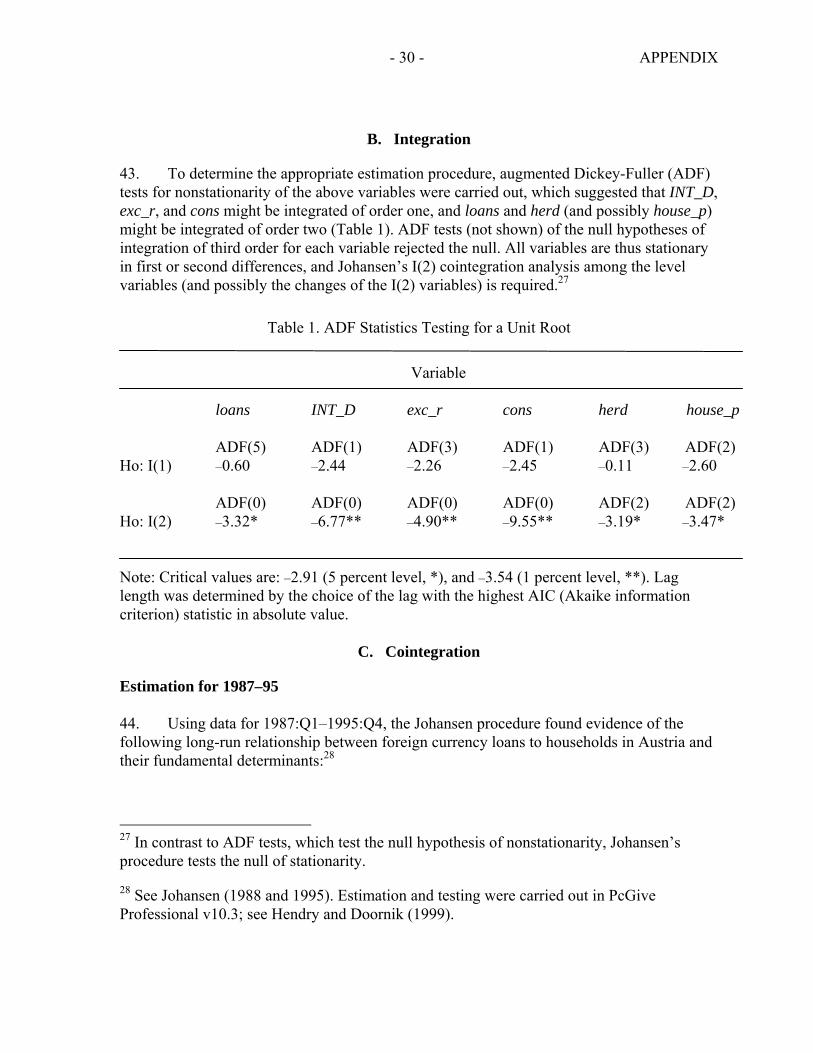
43. To determine the appropriate estimation procedure, augmented Dickey-Fuller (ADF) tests for nonstationarity of the above variables were carried out, which suggested that INT_D, exc_r, and cons might be integrated of order one, and loans and herd (and possibly house_p) might be integrated of order two (Table 1). ADF tests (not shown) of the null hypotheses of integration of third order for each variable rejected the null. All variables are thus stationary in first or second differences, and Johansen’s I(2) cointegration analysis among the level variables (and possibly the changes of the I(2) variables) is required.27
Table 1. ADF Statistics Testing for a Unit Root
Variable loans INT_D exc_r cons herd house_p ADF(5) ADF(1) ADF(3) ADF(1) ADF(3) ADF(2) Ho: I(1) –0.60 –2.44 –2.26 –2.45 –0.11 –2.60 ADF(0) ADF(0) ADF(0) ADF(0) ADF(2) ADF(2) Ho: I(2) –3.32* –6.77** –4.90** –9.55** –3.19* –3.47* Note: Critical values are: –2.91 (5 percent level, *), and –3.54 (1 percent level, **). Lag length was determined by the choice of the lag with the highest AIC (Akaike information criterion) statistic in absolute value.
C. Cointegration
Estimation for 1987–95 44. Using data for 1987:Q1–1995:Q4, the Johansen procedure found evidence of the following long-run relationship between foreign currency loans to households in Austria and their fundamental determinants:28
27 In contrast to ADF tests, which test the null hypothesis of nonstationarity, Johansen’s procedure tests the null of stationarity.
28 See Johansen (1988 and 1995). Estimation and testing were carried out in PcGive Professional v10.3; see Hendry and Doornik (1999).
- 31 - APPENDIX
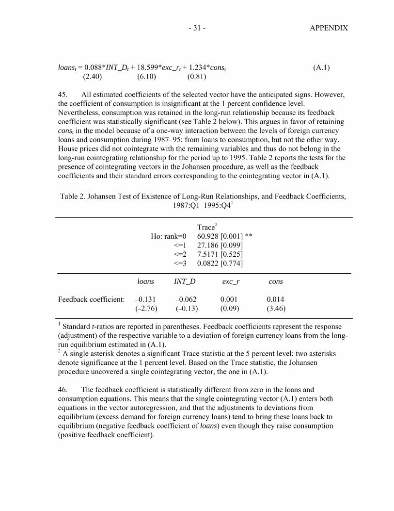
loanst = 0.088*INT_Dt + 18.599*exc_rt + 1.234*const (A.1) (2.40) (6.10) (0.81)
45. All estimated coefficients of the selected vector have the anticipated signs. However, the coefficient of consumption is insignificant at the 1 percent confidence level. Nevertheless, consumption was retained in the long-run relationship because its feedback coefficient was statistically significant (see Table 2 below). This argues in favor of retaining const in the model because of a one-way interaction between the levels of foreign currency loans and consumption during 1987–95: from loans to consumption, but not the other way. House prices did not cointegrate with the remaining variables and thus do not belong in the long-run cointegrating relationship for the period up to 1995. Table 2 reports the tests for the presence of cointegrating vectors in the Johansen procedure, as well as the feedback coefficients and their standard errors corresponding to the cointegrating vector in (A.1).
Table 2. Johansen Test of Existence of Long-Run Relationships, and Feedback Coefficients, 1987:Q1–1995:Q41
Trace2 Ho: rank=0 60.928 [0.001] ** <=1 27.186 [0.099] <=2 7.5171 [0.525] <=3 0.0822 [0.774] loans INT_D exc_r cons Feedback coefficient: –0.131 –0.062 0.001 0.014 (–2.76) (–0.13) (0.09) (3.46) 1 Standard t-ratios are reported in parentheses. Feedback coefficients represent the response (adjustment) of the respective variable to a deviation of foreign currency loans from the long-run equilibrium estimated in (A.1). 2 A single asterisk denotes a significant Trace statistic at the 5 percent level; two asterisks denote significance at the 1 percent level. Based on the Trace statistic, the Johansen procedure uncovered a single cointegrating vector, the one in (A.1). 46. The feedback coefficient is statistically different from zero in the loans and consumption equations. This means that the single cointegrating vector (A.1) enters both equations in the vector autoregression, and that the adjustments to deviations from equilibrium (excess demand for foreign currency loans) tend to bring these loans back to equilibrium (negative feedback coefficient of loans) even though they raise consumption (positive feedback coefficient).
- 32 - APPENDIX
47. The estimated relationship in (A.1) was used to test the hypotheses that both the feedback coefficient for exc_r and the one for INT_D are equal to zero. The test of the hypothesis yielded the following statistic (p value in square brackets):
χ2 (1) = 0.028 [0.986] Based on the large (well in excess of 0.05) p value of the statistic, the null hypothesis cannot be rejected, and the restricted long-run relationship becomes: loanst = 0.094*INT_Dt + 19.001*exc_rt + 1.074*const (A.2) (2.49) (6.07) (0.68) The restricted equation in A.2 was reported in Box 5, together with the unrestricted feedback coefficients for the exchange rate and interest rate differential. 48. The result of the test for weak exogeneity (i.e., that the feedback coefficients of INT_D, exc_r, and cons in Table 2 are jointly equal to zero) is the following:
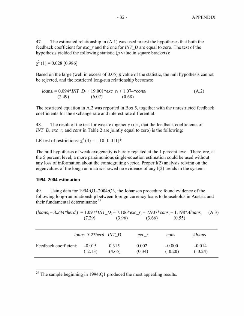
LR test of restrictions: χ2 (4) = 1.10 [0.011]* The null hypothesis of weak exogeneity is barely rejected at the 1 percent level. Therefore, at the 5 percent level, a more parsimonious single-equation estimation could be used without any loss of information about the cointegrating vector. Proper I(2) analysis relying on the eigenvalues of the long-run matrix showed no evidence of any I(2) trends in the system. 1994–2004 estimation 49. Using data for 1994:Q1–2004:Q3, the Johansen procedure found evidence of the following long-run relationship between foreign currency loans to households in Austria and their fundamental determinants: 29
(loanst – 3.244*herdt) = 1.097*INT_Dt + 7.106*exc_rt + 7.907*const – 1.198*∆loanst (A.3) (7.29) (3.96) (3.66) (0.55) loans–3.2*herd INT_D exc_r cons ∆loans Feedback coefficient: –0.015 0.315 0.002 –0.000 –0.014 (–2.13) (4.65) (0.34) (–0.20) (–0.24)
29 The sample beginning in 1994:Q1 produced the most appealing results.
- 33 - APPENDIX
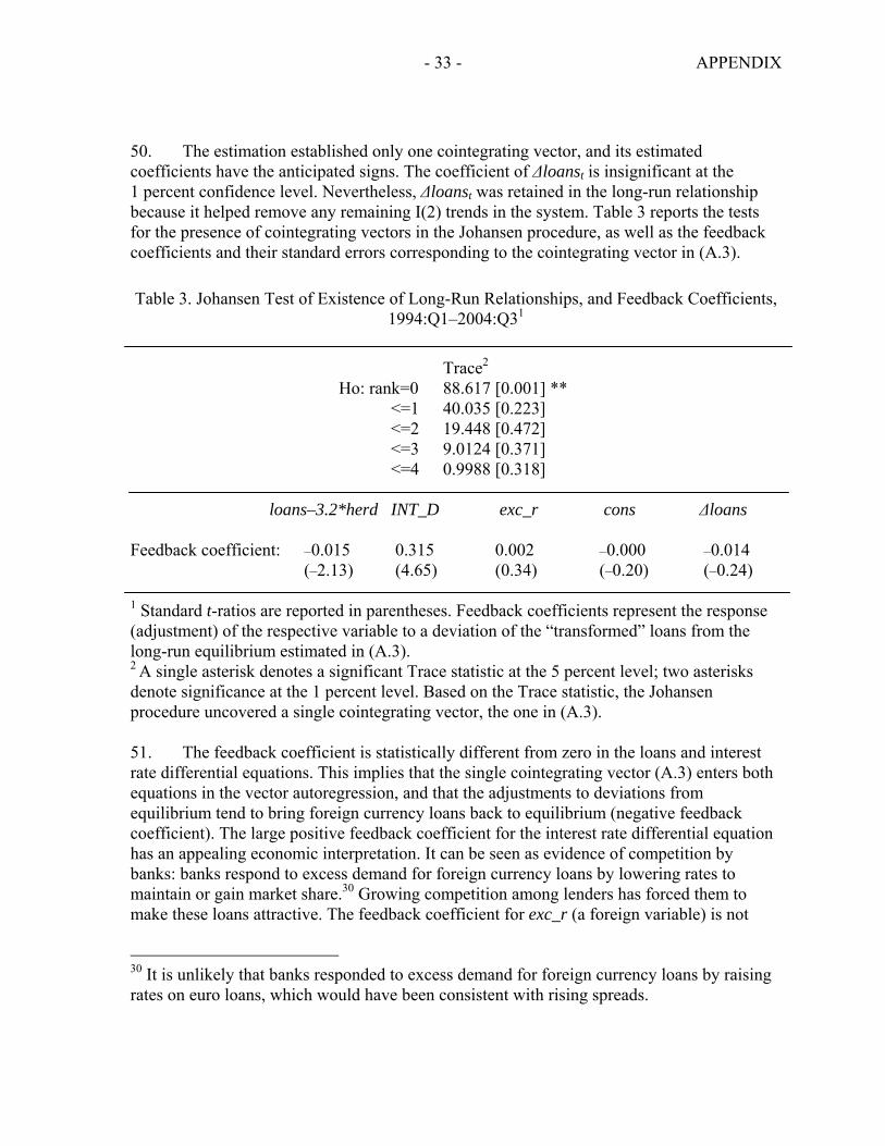
50. The estimation established only one cointegrating vector, and its estimated coefficients have the anticipated signs. The coefficient of ∆loanst is insignificant at the 1 percent confidence level. Nevertheless, ∆loanst was retained in the long-run relationship because it helped remove any remaining I(2) trends in the system. Table 3 reports the tests for the presence of cointegrating vectors in the Johansen procedure, as well as the feedback coefficients and their standard errors corresponding to the cointegrating vector in (A.3).
Table 3. Johansen Test of Existence of Long-Run Relationships, and Feedback Coefficients, 1994:Q1–2004:Q31
Trace2 Ho: rank=0 88.617 [0.001] ** <=1 40.035 [0.223] <=2 19.448 [0.472] <=3 9.0124 [0.371] <=4 0.9988 [0.318] loans–3.2*herd INT_D exc_r cons ∆loans Feedback coefficient: –0.015 0.315 0.002 –0.000 –0.014 (–2.13) (4.65) (0.34) (–0.20) (–0.24) 1 Standard t-ratios are reported in parentheses. Feedback coefficients represent the response (adjustment) of the respective variable to a deviation of the “transformed” loans from the long-run equilibrium estimated in (A.3). 2 A single asterisk denotes a significant Trace statistic at the 5 percent level; two asterisks denote significance at the 1 percent level. Based on the Trace statistic, the Johansen procedure uncovered a single cointegrating vector, the one in (A.3). 51. The feedback coefficient is statistically different from zero in the loans and interest rate differential equations. This implies that the single cointegrating vector (A.3) enters both equations in the vector autoregression, and that the adjustments to deviations from equilibrium tend to bring foreign currency loans back to equilibrium (negative feedback coefficient). The large positive feedback coefficient for the interest rate differential equation has an appealing economic interpretation. It can be seen as evidence of competition by banks: banks respond to excess demand for foreign currency loans by lowering rates to maintain or gain market share.30 Growing competition among lenders has forced them to make these loans attractive. The feedback coefficient for exc_r (a foreign variable) is not
30 It is unlikely that banks responded to excess demand for foreign currency loans by raising rates on euro loans, which would have been consistent with rising spreads.
- 34 - APPENDIX
different from zero, in line with the a priori expectation that exchange rates are determined outside this system.
52. The results of the test for weak exogeneity (i.e., that the feedback coefficients of INT_D, exc_r, cons, and ∆loans in Table 3 are jointly equal to zero) are the following:
LR test of restrictions: χ2 (4) = 31.304 [0.000]** The hypothesis is strongly rejected. Therefore, a more parsimonious single-equation estimation could be used without any loss of information about the cointegrating vector only if the estimates of the vector of coefficients from equation (A.3) are used in the single-equation estimation. 53. The transformed theoretical model shows no evidence of a remaining I(2) trend, confirmed by the eigenvalues of the long-run matrix. Foreign currency loans and the herd variable (both I(2) processes sharing a common I(2) trend) cointegrate to I(1), which in turn cointegrates to I(0) with the other variables in the model. The results confirm that ∆loanst is the common I(2) trend, and its inclusion in the model removes any remaining I(2) components. Since there is no theoretical requirement that the common trend is embedded in equal proportions, the estimation in the unrestricted model found that the common trend was embodied in foreign currency loans and the herd variable with coefficients (1, –3.244).
D. Single-Equation Modeling (Error Correction)
54. This section introduces the long-run dynamics established in (A.3) into a single-equation, conditional, and parsimonious model for loans to households in foreign currency in Austria that encompasses both short- and long-run dynamics. The short-run dynamics are derived from the following vector of changes in the log-levels of the variables (levels for INT_D) used so far in the analysis:
Is = {∆vt-j}; j = 0, 1…, where vt-j is the vector of all variables (contemporaneous and lagged) used so far, with the addition of two new stationary variables, orthogonal to the existing repressors. These are: ∆house_p = Quarter-on-quarter change of house prices, and DUMMY = Dummy variable for policy measures: D = 0 for 1994:Q1–2003:Q2;
and D = 1 for 2003:Q3–2004:Q3. 55. An error-correction model for loans to Austrian households in foreign currency was estimated using quarterly data over 1994:Q1–2004:Q3. Estimation began from a general specification with several variables and lags, which also included the vector Is and the deviations of foreign currency loans from the long-run relationship (A.3) established above. Subsequently, parameter tests were performed (mostly zero restrictions) to reduce the model
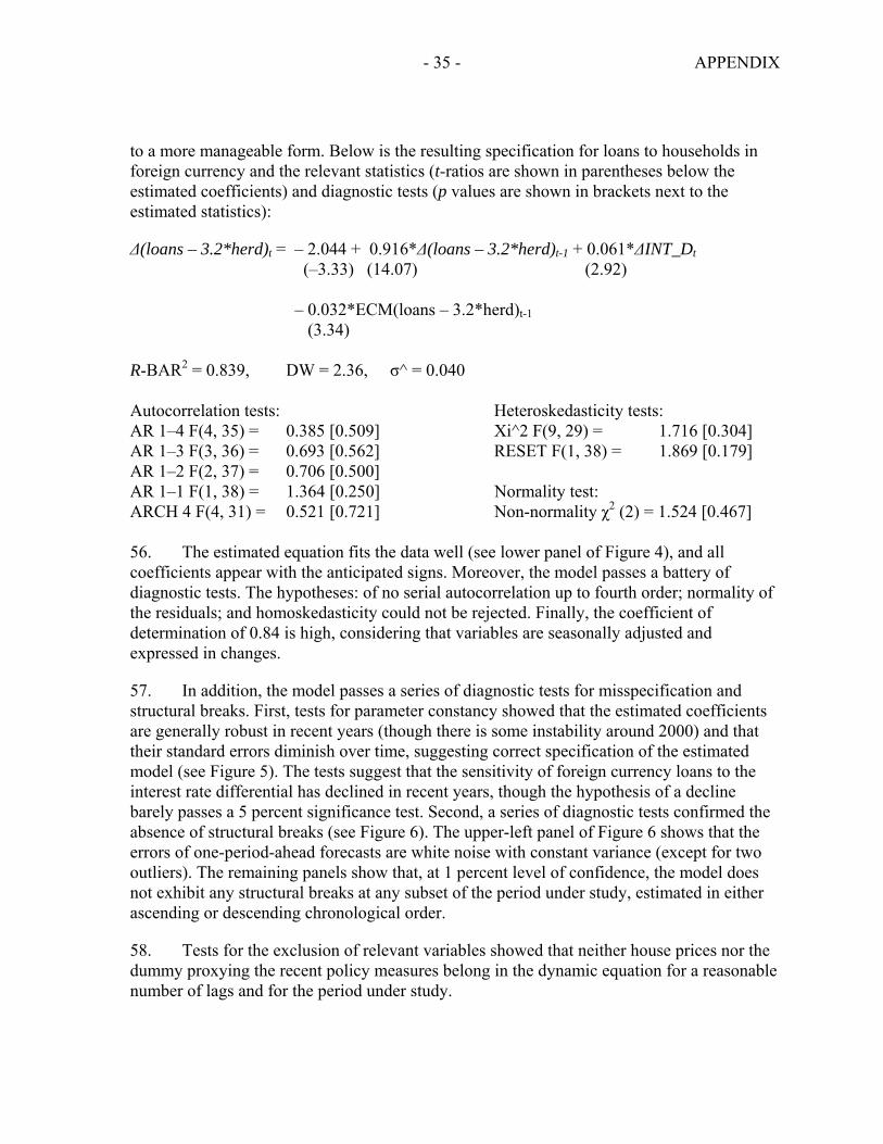
- 35 - APPENDIX
to a more manageable form. Below is the resulting specification for loans to households in foreign currency and the relevant statistics (t-ratios are shown in parentheses below the estimated coefficients) and diagnostic tests (p values are shown in brackets next to the estimated statistics):
∆(loans – 3.2*herd)t = – 2.044 + 0.916*∆(loans – 3.2*herd)t-1 + 0.061*∆INT_Dt (–3.33) (14.07) (2.92) – 0.032*ECM(loans – 3.2*herd)t-1 (3.34) R-BAR2 = 0.839, DW = 2.36, σ^ = 0.040 Autocorrelation tests: Heteroskedasticity tests: AR 1–4 F(4, 35) = 0.385 [0.509] Xi^2 F(9, 29) = 1.716 [0.304] AR 1–3 F(3, 36) = 0.693 [0.562] RESET F(1, 38) = 1.869 [0.179] AR 1–2 F(2, 37) = 0.706 [0.500] AR 1–1 F(1, 38) = 1.364 [0.250] Normality test: ARCH 4 F(4, 31) = 0.521 [0.721] Non-normality χ2 (2) = 1.524 [0.467] 56. The estimated equation fits the data well (see lower panel of Figure 4), and all coefficients appear with the anticipated signs. Moreover, the model passes a battery of diagnostic tests. The hypotheses: of no serial autocorrelation up to fourth order; normality of the residuals; and homoskedasticity could not be rejected. Finally, the coefficient of determination of 0.84 is high, considering that variables are seasonally adjusted and expressed in changes.
57. In addition, the model passes a series of diagnostic tests for misspecification and structural breaks. First, tests for parameter constancy showed that the estimated coefficients are generally robust in recent years (though there is some instability around 2000) and that their standard errors diminish over time, suggesting correct specification of the estimated model (see Figure 5). The tests suggest that the sensitivity of foreign currency loans to the interest rate differential has declined in recent years, though the hypothesis of a decline barely passes a 5 percent significance test. Second, a series of diagnostic tests confirmed the absence of structural breaks (see Figure 6). The upper-left panel of Figure 6 shows that the errors of one-period-ahead forecasts are white noise with constant variance (except for two outliers). The remaining panels show that, at 1 percent level of confidence, the model does not exhibit any structural breaks at any subset of the period under study, estimated in either ascending or descending chronological order.
58. Tests for the exclusion of relevant variables showed that neither house prices nor the dummy proxying the recent policy measures belong in the dynamic equation for a reasonable number of lags and for the period under study.
- 36 -
References Alevy, J. E., M. S. Haigh, and J. A. List, 2003, “Information Cascades: Evidence from a
Field Experiment with Financial Market Professionals,” Department of Agricultural and Resource, Economics Working Paper 03-15 (College Park: The University of Maryland).
Ball, M., 2004, “Austria,” RICS European Housing Market Review 2004, Chapter 4,
pp. 17-27 (London: RICS Europe). Banerjee, A. V., 1992, “A Simple Model of Herd Behavior,” The Quarterly Journal of
Economics, Vol. CVII(3), pp. 797-817. Braumann, B., 2004, “Tu Felix Austria: Evidence for a De-celerator in Financial Reform,”
International Economics and Economic Policy, Vol. 1(1), pp. 53-72. Drehmann, M., J. Oechssler, and A. Roider, 2003, “Herding and Contrarian Behavior in
Financial Markets—An Internet Experiment,” Discussion Paper (London: Bank of England).
Fiess, N., and R. MacDonald, 2001, “The Instability of the Money Demand Function: an I(2)
Interpretation,” Oxford Bulletin of Economics and Statistics, Vol. 63(4), pp. 475-95. Giovannini, A., and B. Turtelboom, 1992, “Currency Substitution,” NBER Working Paper
No. 4232 (Cambridge, MA: National Bureau of Economic Research). Gnan, E., 1994, “Austria’s Hard Currency Policy and European Monetary Integration,”
De Pecunia, Vol. 6(3), pp. 27-72. Hendry, D. F., and J. A. Doornik, 1999, Empirical Econometric Modeling Using PcGive,
(West Wickham: Timberland Consultants Ltd.). Hofmann, B., 2001, “The Determinants of Private Sector Credit in Industrialized Countries:
Do Property Prices Matter?” BIS Working Paper 108 (Basel: Bank for International Settlements).
IMF, 2004, “Austria: Financial System Stability Assessment,” IMF Country Report
No. 04/238 (Washington: International Monetary Fund). Johansen, S., 1988, “Statistical Analysis of Cointegration Vectors,” Journal of Economic Dynamics and Control, Vol. 12, pp. 231–254. —————, 1992, “An I(2) Cointegration Analysis of the Purchasing Power Parity Between
Australia and the United States,” Article 9 in C. P. Hargreaves (editor) Macroeconomic Modelling of the Long Run, p.p. 229-48 (Aldershot: Edward Elgar Publishing Limited).
- 37 -
—————, 1995, Likelihood-based Inference in Cointegrated Vector Autoregressive
Models, (Oxford: Oxford University Press).
Kaufmann, S., and M. T. Valderrama, 2004, “Modeling Credit Aggregates,” OeNB Working Paper 90 (Vienna: Oesterreichische Nationalbank).
Kingston, G., 1995, “The Foreign Currency Loans Affair: An Economist’s Perspective,”
School of Economics Discussion Paper 95/10 (Sydney: The University of New South Wales).
Komárek, L., and M. Melecký M., 2003, “Currency Substitution in a Transitional Economy
with an Application to the Czech Republic,” Eastern European Economics, Vol. 41(4), pp. 72-99.
Levi-Faur, D., 2002, “Herding Towards a New Convention: On Herds, Shepherds, and Lost
Sheep in the Liberalization of the Telecommunications and Electricity Industries,” Nuffield College Working Paper in Politics 6 (Oxford: University of Oxford).
Luca, A., and I. Petrova, 2003, “Is Credit Dollarization Driven by Firms or Banks?”
unpublished (Lancing: Michigan State University). Maggioni, M. A., 2004, “The rise and Fall of Industrial clusters: Technology and the Life
Cycle of Regions,” Instut d’Economia de Barcelona Working Paper 2004/6 (Barcelona: University of Barcelona).
Montier, J., 2002, Behavioural Finance: Insights into Irrational Minds and Markets
(Chichester: John Wiley & Sons Ltd.) OeNB, 2003, Financial Stability Report 5, pp. 26-28 (Vienna: Oesterreichische
Nationalbank). Tsoularis, A., 2001, “Analysis of Logistic Growth Models,” Research Letters in Informatics
and Mathematical Sciences, Vol. 2, pp. 23-46. Tzanninis, D., 2002, “Why Has U.K. Household Consumption Been so Strong?” in United
Kingdom: Selected Issues, IMF Country Report No. 02/46 (Washington: International Monetary Fund).
Waschiczek, W., 2002, “Foreign Currency Loans in Austria—Efficiency and Risk
Considerations,” in Financial Stability Report 4, OeNB, pp. 83-99 (Vienna: Oesterreichische Nationalbank).
Yoshifuji, S., and H. Demizu, 1998, “A Study of the Mechanism of Stress/Shock Movements
in Financial Markets,” unpublished (Tokyo: The Bank of Tokyo—Mitsubishi, Ltd.).
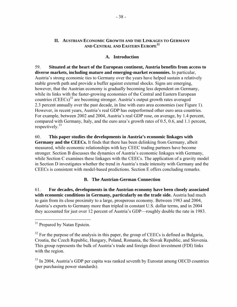
- 38 -
II. AUSTRIAN ECONOMIC GROWTH AND THE LINKAGES TO GERMANY AND CENTRAL AND EASTERN EUROPE31
A. Introduction
59. Situated at the heart of the European continent, Austria benefits from access to diverse markets, including mature and emerging-market economies. In particular, Austria’s strong economic ties to Germany over the years have helped sustain a relatively stable growth path and provide a buffer against external shocks. Signs are emerging, however, that the Austrian economy is gradually becoming less dependent on Germany, while its links with the faster-growing economies of the Central and Eastern European countries (CEECs)32 are becoming stronger. Austria’s output growth rates averaged 2.3 percent annually over the past decade, in line with euro area economies (see Figure 1). However, in recent years, Austria’s real GDP has outperformed other euro area countries. For example, between 2002 and 2004, Austria’s real GDP rose, on average, by 1.4 percent, compared with Germany, Italy, and the euro area’s growth rates of 0.5, 0.6, and 1.1 percent, respectively.33
60. This paper studies the developments in Austria’s economic linkages with Germany and the CEECs. It finds that there has been delinking from Germany, albeit measured, while economic relationships with key CEEC trading partners have become stronger. Section B discusses the dynamics of Austria’s economic linkages with Germany, while Section C examines these linkages with the CEECs. The application of a gravity model in Section D investigates whether the trend in Austria’s trade intensity with Germany and the CEECs is consistent with model-based predictions. Section E offers concluding remarks.
B. The Austrian-German Connection
61. For decades, developments in the Austrian economy have been closely associated with economic conditions in Germany, particularly on the trade side. Austria had much to gain from its close proximity to a large, prosperous economy. Between 1983 and 2004, Austria’s exports to Germany more than tripled in constant U.S. dollar terms, and in 2004 they accounted for just over 12 percent of Austria’s GDP—roughly double the rate in 1983.
31 Prepared by Natan Epstein.
32 For the purpose of the analysis in this paper, the group of CEECs is defined as Bulgaria, Croatia, the Czech Republic, Hungary, Poland, Romania, the Slovak Republic, and Slovenia. This group represents the bulk of Austria’s trade and foreign direct investment (FDI) links with the region.
33 In 2004, Austria’s GDP per capita was ranked seventh by Eurostat among OECD countries (per purchasing power standards).
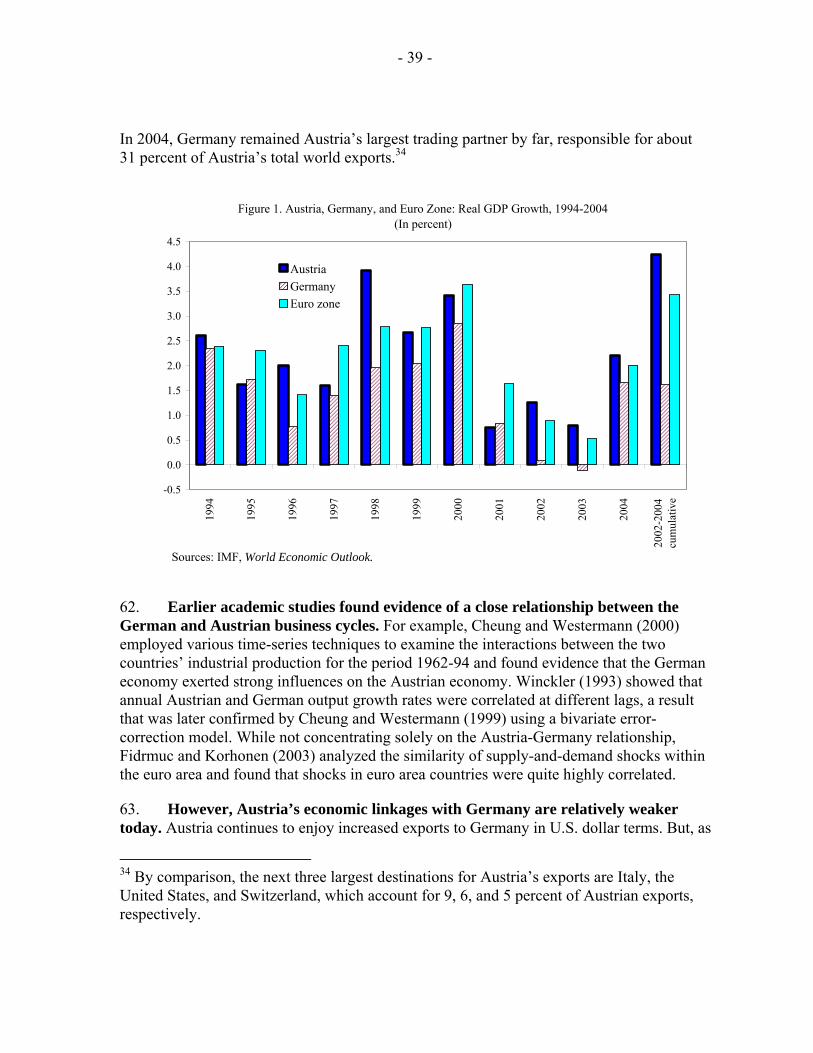
- 39 -
In 2004, Germany remained Austria’s largest trading partner by far, responsible for about 31 percent of Austria’s total world exports.34
62. Earlier academic studies found evidence of a close relationship between the German and Austrian business cycles. For example, Cheung and Westermann (2000) employed various time-series techniques to examine the interactions between the two countries’ industrial production for the period 1962-94 and found evidence that the German economy exerted strong influences on the Austrian economy. Winckler (1993) showed that annual Austrian and German output growth rates were correlated at different lags, a result that was later confirmed by Cheung and Westermann (1999) using a bivariate error-correction model. While not concentrating solely on the Austria-Germany relationship, Fidrmuc and Korhonen (2003) analyzed the similarity of supply-and-demand shocks within the euro area and found that shocks in euro area countries were quite highly correlated.
63. However, Austria’s economic linkages with Germany are relatively weaker today. Austria continues to enjoy increased exports to Germany in U.S. dollar terms. But, as
34 By comparison, the next three largest destinations for Austria’s exports are Italy, the United States, and Switzerland, which account for 9, 6, and 5 percent of Austrian exports, respectively.
Figure 1. Austria, Germany, and Euro Zone: Real GDP Growth, 1994-2004(In percent)
-0.5
0.0
0.5
1.0
1.5
2.0
2.5
3.0
3.5
4.0
4.5
1994
1995
1996
1997
1998
1999
2000
2001
2002
2003
2004
2002
-200
4cu
mul
ativ
e
AustriaGermanyEuro zone
Sources: IMF, World Economic Outlook.
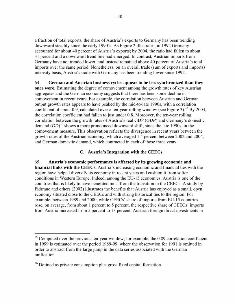
- 40 -
a fraction of total exports, the share of Austria’s exports to Germany has been trending downward steadily since the early 1990’s. As Figure 2 illustrates, in 1992 Germany accounted for about 40 percent of Austria’s exports; by 2004, the ratio had fallen to about 31 percent and a downward trend line had emerged. In contrast, Austrian imports from Germany have not trended lower, and instead remained above 40 percent of Austria’s total imports over the same period. Nonetheless, on an overall trade (sum of exports and imports) intensity basis, Austria’s trade with Germany has been trending lower since 1992.
64. German and Austrian business cycles appear to be less synchronized than they once were. Estimating the degree of comovement among the growth rates of key Austrian aggregates and the German economy suggests that there has been some decline in comovement in recent years. For example, the correlation between Austrian and German output growth rates appears to have peaked by the mid-to-late 1990s, with a correlation coefficient of about 0.9, calculated over a ten-year rolling window (see Figure 3).35 By 2004, the correlation coefficient had fallen to just under 0.8. Moreover, the ten-year rolling correlation between the growth rates of Austria’s real GDP (GDP) and Germany’s domestic demand (DD)36 shows a more pronounced downward shift, since the late 1990s, in the comovement measure. This observation reflects the divergence in recent years between the growth rates of the Austrian economy, which averaged 1.4 percent between 2002 and 2004, and German domestic demand, which contracted in each of those three years.
C. Austria’s Integration with the CEECs
65. Austria’s economic performance is affected by its growing economic and financial links with the CEECs. Austria’s increasing economic and financial ties with the region have helped diversify its economy in recent years and cushion it from softer conditions in Western Europe. Indeed, among the EU-15 economies, Austria is one of the countries that is likely to have benefited most from the transition in the CEECs. A study by Fidrmuc and others (2002) illustrates the benefits that Austria has enjoyed as a small, open economy situated close to the CEECs and with strong historical ties to the region. For example, between 1989 and 2000, while CEECs’ share of imports from EU-15 countries rose, on average, from about 1 percent to 5 percent, the respective share of CEECs’ imports from Austria increased from 5 percent to 13 percent. Austrian foreign direct investments in
35 Computed over the previous ten-year window; for example, the 0.89 correlation coefficient in 1999 is estimated over the period 1989-99, where the observation for 1991 is omitted in order to abstract from the large jump in the data series associated with the German unification.
36 Defined as private consumption plus gross fixed capital formation.
- 41 -
Figure 2. Austria's Trade Intensity with Germany, 1992-2004(In percent)
30
32
34
36
38
40
42
44
46
1992
1993
1994
1995
1996
1997
1998
1999
2000
2001
2002
2003
2004
Exports to Germany(as a share of total Austrian exports)
Imports from Germany(as a share of total Austrian imports
Trade intensity (exports plus imports)
Source: IMF, Direction of Trade Statistics.
Figure 3. Austria and Germany: Output Comovement, 1993-2004 (Ten-year rolling correlation)
0.60
0.65
0.70
0.75
0.80
0.85
0.90
0.95
1993 1994 1995 1996 1997 1998 1999 2000 2001 2002 2003 2004
Austria GDP - Germany GDP
Austria GDP - Germany DD
Source: IMF, World Economic Outlook.
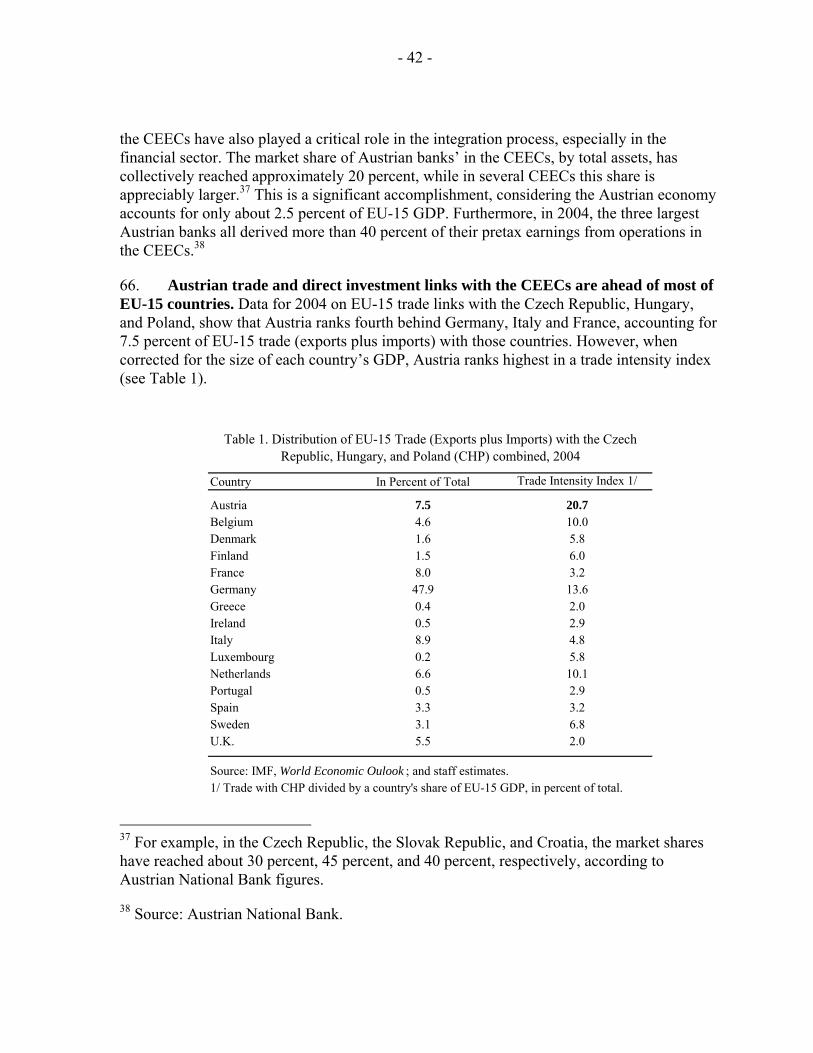
- 42 -
the CEECs have also played a critical role in the integration process, especially in the financial sector. The market share of Austrian banks’ in the CEECs, by total assets, has collectively reached approximately 20 percent, while in several CEECs this share is appreciably larger.37 This is a significant accomplishment, considering the Austrian economy accounts for only about 2.5 percent of EU-15 GDP. Furthermore, in 2004, the three largest Austrian banks all derived more than 40 percent of their pretax earnings from operations in the CEECs.38
66. Austrian trade and direct investment links with the CEECs are ahead of most of EU-15 countries. Data for 2004 on EU-15 trade links with the Czech Republic, Hungary, and Poland, show that Austria ranks fourth behind Germany, Italy and France, accounting for 7.5 percent of EU-15 trade (exports plus imports) with those countries. However, when corrected for the size of each country’s GDP, Austria ranks highest in a trade intensity index (see Table 1).
37 For example, in the Czech Republic, the Slovak Republic, and Croatia, the market shares have reached about 30 percent, 45 percent, and 40 percent, respectively, according to Austrian National Bank figures.
38 Source: Austrian National Bank.
Country In Percent of Total Trade Intensity Index 1/
Austria 7.5 20.7Belgium 4.6 10.0Denmark 1.6 5.8Finland 1.5 6.0France 8.0 3.2Germany 47.9 13.6Greece 0.4 2.0Ireland 0.5 2.9Italy 8.9 4.8Luxembourg 0.2 5.8Netherlands 6.6 10.1Portugal 0.5 2.9Spain 3.3 3.2Sweden 3.1 6.8U.K. 5.5 2.0
1/ Trade with CHP divided by a country's share of EU-15 GDP, in percent of total.
Table 1. Distribution of EU-15 Trade (Exports plus Imports) with the Czech Republic, Hungary, and Poland (CHP) combined, 2004
Source: IMF, World Economic Oulook ; and staff estimates.
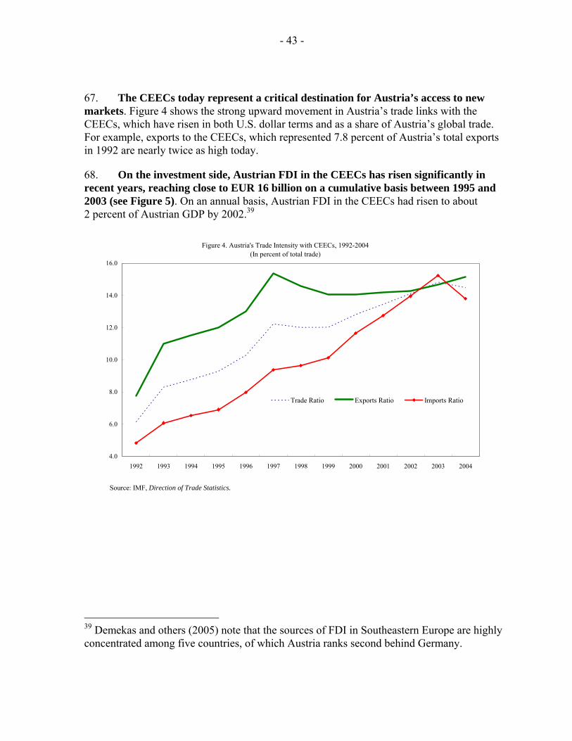
- 43 -
67. The CEECs today represent a critical destination for Austria’s access to new markets. Figure 4 shows the strong upward movement in Austria’s trade links with the CEECs, which have risen in both U.S. dollar terms and as a share of Austria’s global trade. For example, exports to the CEECs, which represented 7.8 percent of Austria’s total exports in 1992 are nearly twice as high today.
68. On the investment side, Austrian FDI in the CEECs has risen significantly in recent years, reaching close to EUR 16 billion on a cumulative basis between 1995 and 2003 (see Figure 5). On an annual basis, Austrian FDI in the CEECs had risen to about 2 percent of Austrian GDP by 2002.39
39 Demekas and others (2005) note that the sources of FDI in Southeastern Europe are highly concentrated among five countries, of which Austria ranks second behind Germany.
Figure 4. Austria's Trade Intensity with CEECs, 1992-2004(In percent of total trade)
4.0
6.0
8.0
10.0
12.0
14.0
16.0
1992 1993 1994 1995 1996 1997 1998 1999 2000 2001 2002 2003 2004
Trade Ratio Exports Ratio Imports Ratio
Source: IMF, Direction of Trade Statistics.
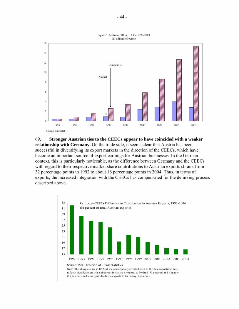
- 44 -
69. Stronger Austrian ties to the CEECs appear to have coincided with a weaker relationship with Germany. On the trade side, it seems clear that Austria has been successful in diversifying its export markets in the direction of the CEECs, which have become an important source of export earnings for Austrian businesses. In the German context, this is particularly noticeable, as the difference between Germany and the CEECs with regard to their respective market share contributions to Austrian exports shrank from 32 percentage points in 1992 to about 16 percentage points in 2004. Thus, in terms of exports, the increased integration with the CEECs has compensated for the delinking process described above.
Figure 5. Austrian FDI in CEECs, 1995-2003(In billions of euros)
0
2
4
6
8
10
12
14
16
1995 1996 1997 1998 1999 2000 2001 2002 2003
Annual
Cumulative
Source: Eurostat.
15
17
19
21
23
25
27
29
31
33
1992 1993 1994 1995 1996 1997 1998 1999 2000 2001 2002 2003 2004
Germany--CEECs Difference in Contribution to Austrian Exports, 1992-2004(In percent of total Austrian exports)
Source: IMF Direction of Trade Statistics.No te : The s harp dec line in 1997, which s ubs equently reverted back to the do wnward trend line , re flec ts s ignificant gro wth in tha t year in Aus tria ’s expo rts to P o land (50 percent) and Hungary (25 pe rcent), and a margina l dec line in expo rts to Germany (5 percent).
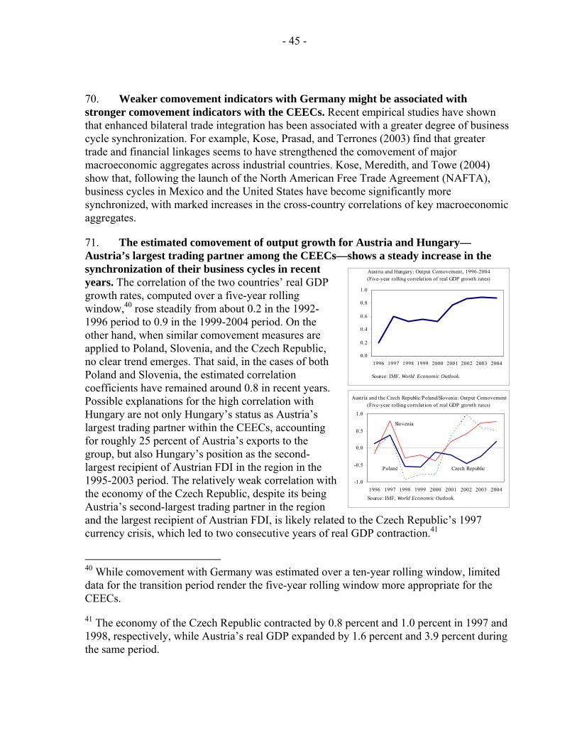
- 45 -
70. Weaker comovement indicators with Germany might be associated with stronger comovement indicators with the CEECs. Recent empirical studies have shown that enhanced bilateral trade integration has been associated with a greater degree of business cycle synchronization. For example, Kose, Prasad, and Terrones (2003) find that greater trade and financial linkages seems to have strengthened the comovement of major macroeconomic aggregates across industrial countries. Kose, Meredith, and Towe (2004) show that, following the launch of the North American Free Trade Agreement (NAFTA), business cycles in Mexico and the United States have become significantly more synchronized, with marked increases in the cross-country correlations of key macroeconomic aggregates.
71. The estimated comovement of output growth for Austria and Hungary—Austria’s largest trading partner among the CEECs—shows a steady increase in the synchronization of their business cycles in recent years. The correlation of the two countries’ real GDP growth rates, computed over a five-year rolling window,40 rose steadily from about 0.2 in the 1992-1996 period to 0.9 in the 1999-2004 period. On the other hand, when similar comovement measures are applied to Poland, Slovenia, and the Czech Republic, no clear trend emerges. That said, in the cases of both Poland and Slovenia, the estimated correlation coefficients have remained around 0.8 in recent years. Possible explanations for the high correlation with Hungary are not only Hungary’s status as Austria’s largest trading partner within the CEECs, accounting for roughly 25 percent of Austria’s exports to the group, but also Hungary’s position as the second-largest recipient of Austrian FDI in the region in the 1995-2003 period. The relatively weak correlation with the economy of the Czech Republic, despite its being Austria’s second-largest trading partner in the region and the largest recipient of Austrian FDI, is likely related to the Czech Republic’s 1997 currency crisis, which led to two consecutive years of real GDP contraction.41
40 While comovement with Germany was estimated over a ten-year rolling window, limited data for the transition period render the five-year rolling window more appropriate for the CEECs.
41 The economy of the Czech Republic contracted by 0.8 percent and 1.0 percent in 1997 and 1998, respectively, while Austria’s real GDP expanded by 1.6 percent and 3.9 percent during the same period.
0.0
0.2
0.4
0.6
0.8
1.0
1996 1997 1998 1999 2000 2001 2002 2003 2004
Austria and Hungary: Output Comovement, 1996-2004 (Five-year rolling correlation of real GDP growth rates)
Source: IMF, World Economic Outlook.
-1.0
-0.5
0.0
0.5
1.0
1996 1997 1998 1999 2000 2001 2002 2003 2004
Poland
Slovenia
Source: IMF, World Economic Outlook.
Austria and the Czech Republic/Poland/Slovenia: Output Comovement (Five-year rolling correlation of real GDP growth rates)
Czech Republic
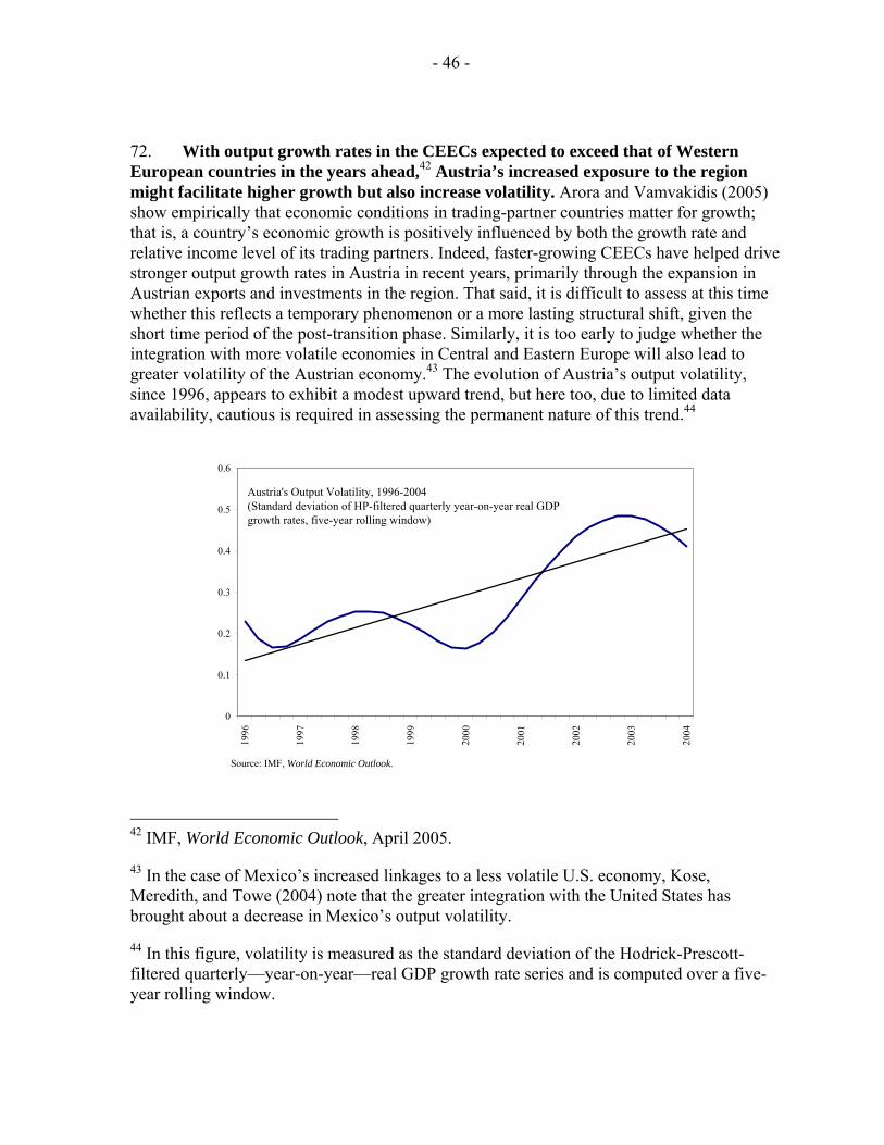
- 46 -
72. With output growth rates in the CEECs expected to exceed that of Western European countries in the years ahead,42 Austria’s increased exposure to the region might facilitate higher growth but also increase volatility. Arora and Vamvakidis (2005) show empirically that economic conditions in trading-partner countries matter for growth; that is, a country’s economic growth is positively influenced by both the growth rate and relative income level of its trading partners. Indeed, faster-growing CEECs have helped drive stronger output growth rates in Austria in recent years, primarily through the expansion in Austrian exports and investments in the region. That said, it is difficult to assess at this time whether this reflects a temporary phenomenon or a more lasting structural shift, given the short time period of the post-transition phase. Similarly, it is too early to judge whether the integration with more volatile economies in Central and Eastern Europe will also lead to greater volatility of the Austrian economy.43 The evolution of Austria’s output volatility, since 1996, appears to exhibit a modest upward trend, but here too, due to limited data availability, cautious is required in assessing the permanent nature of this trend.44
42 IMF, World Economic Outlook, April 2005.
43 In the case of Mexico’s increased linkages to a less volatile U.S. economy, Kose, Meredith, and Towe (2004) note that the greater integration with the United States has brought about a decrease in Mexico’s output volatility.
44 In this figure, volatility is measured as the standard deviation of the Hodrick-Prescott-filtered quarterly—year-on-year—real GDP growth rate series and is computed over a five-year rolling window.
0
0.1
0.2
0.3
0.4
0.5
0.6
1996
1997
1998
1999
2000
2001
2002
2003
2004
Austria's Output Volatility, 1996-2004(Standard deviation of HP-filtered quarterly year-on-year real GDP growth rates, five-year rolling window)
Source: IMF, World Economic Outlook.
- 47 -
D. Gravity Model Application
73. The objective of employing the gravity model in this paper is to assess, econometrically, whether Austria’s trade patterns with Germany and Hungary are consistent with estimated model predictions, and whether those estimates reflect the process of delinking and integration discussed above.45 The gravity model of international trade has been used extensively in empirical studies analyzing patterns of bilateral trade. Eichengreen and Irwin (1998) noted that what made the application of the gravity model so popular was its ability to explain the variation in bilateral trade flows across a wide variety of countries and time periods, and that “few aggregate economic relationships are as robust.”
74. The typical gravity model specification relates bilateral trade to GDP in each country, their per capita incomes, and the distance between them. An expanded version of this model includes additional variables typically reflecting geographical, cultural, and historical factors that have been found to be statistically relevant for bilateral trade patterns (e.g., area size of country and dummy variables for contiguity, membership in regional trade arrangements, common language, landlocked vs. island economies, history of colonization). On a bilateral basis, trade between countries i and j , in year t , is estimated as a log-linear function and is generally given by
( ) ( ) ( ) ( )0 1 2 31
ln ln ln ln ,n
ijt i j i j ij z ijtt tz
Trade GDPGDP GDPpc GDPpc Dist Xβ β β β θ ε=
= + + + + +∑
where ijTrade is the value of bilateral trade , i jGDPGDP is the product of the two countries’ real GDPs, i jGDPpc GDPpc is the product of the two countries’ per capita income, ijDist is the straight-line distance between the economic centers of the two countries,
1
n
zz
Xθ=∑ represents the set of geographical/cultural/historical variables, and ε is a randomly
distributed error term. As trade is expected to rise with GDP and per capita income, and to fall with distance, 1β and 2β ought to reflect a positive estimate, while 3β should reflect a negative estimate.
75. The analysis below draws on two separate panel data sets, Rose (2004) and Bussière, Fidrmuc, and Schantz (BFS, 2005).46 The former is a very large panel, covering 175 countries for the period 1950-99, while the latter comprises 61 countries for the period 45 We use Hungary as a representative country for the CEECs, since it is Austria’s key trading-partner in the region and long-run data for most of the other countries in the region are more limited.
46 In Rose (2004), the gravity model is used to analyze the effects of multilateral trade agreements on trade, while in BFS (2005) the gravity model is adopted to analyze trade linkages between the euro area and Central and Southeastern Europe.
- 48 -
1980-2003.47 The BFS data set is used to extend the analysis through the period 1998-2003. The cross-country time-series data in both panels include annual observations for the respective periods. Trade is defined by merchandise trade.
76. Based on the equation depicted above, a gravity model is estimated with an ordinary least squares (OLS) regression.48 The results are presented in Table 2. The first column reflects the results using the Rose data for 1950-97, and the second column presents the results using the BFS data for 1980-2003. The results in the first column are generated from a close variant of the “benchmark” regression in Rose (2004). The regression includes dummies for free trade areas (EU, NAFTA, Mercosur, and ASEAN) and excludes the dummies for membership in the GATT/WTO, which Rose had found to be statistically insignificant. In the regression using the BFS data, some of the geographical and historical dummies that entered the former regression (e.g., history of colonization, landlocked vs. island economies) are missing, but the coefficients on key variables—real GDP, real GDP per capita, distance, and contiguity—are nonetheless statistically the same. Both columns reflect OLS estimations with time-year effects. For a robustness check, the model was also estimated with country-specific fixed effects and random effects, and the results were statistically similar.
77. The results are broadly consistent with those found in the literature and track closely the estimated coefficients in Rose (2004) and BFS (2005). Indeed, the results are consistent with the model’s prediction: bilateral trade rises with real GDP and per capita income and falls with distance, and the coefficients on these three variables are statistically significant. Additionally, some of the key geographical and cultural variables also appear to be explained well by the model, such as the positive coefficients on contiguity and common language.
78. Applying the estimated coefficients from Table 2 to the corresponding bilateral trade equations allows us to calculate the predicted levels of trade according to the model. In turn, these levels can be used to examine whether the actual (observed) trade levels are below or above the model-based predictions. If the observed levels are below predicted levels, one could expect trade to grow faster than would be predicted by real GDP growth rates, per-capita income, distance, and so forth. Similarly, if the observed levels are above the predicted levels, one could expect trade to grow more slowly than would be predicted by the gravity model’s explanatory variables. As with any model application, one should be aware of the limitations of the model. In particular, the residual may not fully capture all the intrinsic elements that are specific to Austria’s bilateral trade patterns.
47 For data consistency reasons, we used the Rose panel data through 1997. 48 For definitions of the variables included in
1
n
zz
Xθ=∑ , see the Appendix.
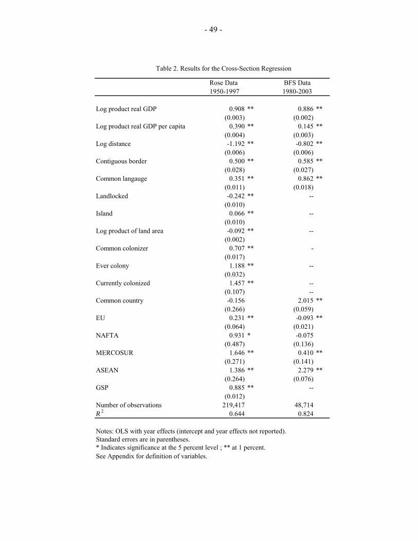
- 49 -
Table 2. Results for the Cross-Section Regression
Rose Data BFS Data1950-1997 1980-2003
Log product real GDP 0.908 ** 0.886 **(0.003) (0.002)
Log product real GDP per capita 0.390 ** 0.145 **(0.004) (0.003)
Log distance -1.192 ** -0.802 **(0.006) (0.006)
Contiguous border 0.500 ** 0.585 **(0.028) (0.027)
Common langauge 0.351 ** 0.862 **(0.011) (0.018)
Landlocked -0.242 ** --(0.010)
Island 0.066 ** --(0.010)
Log product of land area -0.092 ** --(0.002)
Common colonizer 0.707 ** -(0.017)
Ever colony 1.188 ** --(0.032)
Currently colonized 1.457 ** --(0.107) --
Common country -0.156 2.015 **(0.266) (0.059)
EU 0.231 ** -0.093 **(0.064) (0.021)
NAFTA 0.931 * -0.075(0.487) (0.136)
MERCOSUR 1.646 ** 0.410 **(0.271) (0.141)
ASEAN 1.386 ** 2.279 **(0.264) (0.076)
GSP 0.885 ** --(0.012)
Number of observations 219,417 48,714R 2 0.644 0.824
Notes: OLS with year effects (intercept and year effects not reported).Standard errors are in parentheses. * Indicates significance at the 5 percent level ; ** at 1 percent.See Appendix for definition of variables.
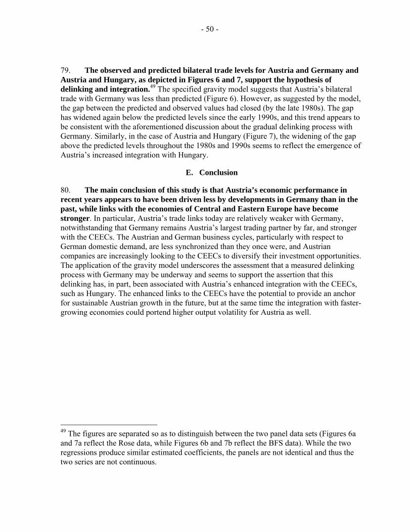
- 50 -
79. The observed and predicted bilateral trade levels for Austria and Germany and Austria and Hungary, as depicted in Figures 6 and 7, support the hypothesis of delinking and integration.49 The specified gravity model suggests that Austria’s bilateral trade with Germany was less than predicted (Figure 6). However, as suggested by the model, the gap between the predicted and observed values had closed (by the late 1980s). The gap has widened again below the predicted levels since the early 1990s, and this trend appears to be consistent with the aforementioned discussion about the gradual delinking process with Germany. Similarly, in the case of Austria and Hungary (Figure 7), the widening of the gap above the predicted levels throughout the 1980s and 1990s seems to reflect the emergence of Austria’s increased integration with Hungary.
E. Conclusion
80. The main conclusion of this study is that Austria’s economic performance in recent years appears to have been driven less by developments in Germany than in the past, while links with the economies of Central and Eastern Europe have become stronger. In particular, Austria’s trade links today are relatively weaker with Germany, notwithstanding that Germany remains Austria’s largest trading partner by far, and stronger with the CEECs. The Austrian and German business cycles, particularly with respect to German domestic demand, are less synchronized than they once were, and Austrian companies are increasingly looking to the CEECs to diversify their investment opportunities. The application of the gravity model underscores the assessment that a measured delinking process with Germany may be underway and seems to support the assertion that this delinking has, in part, been associated with Austria’s enhanced integration with the CEECs, such as Hungary. The enhanced links to the CEECs have the potential to provide an anchor for sustainable Austrian growth in the future, but at the same time the integration with faster-growing economies could portend higher output volatility for Austria as well.
49 The figures are separated so as to distinguish between the two panel data sets (Figures 6a and 7a reflect the Rose data, while Figures 6b and 7b reflect the BFS data). While the two regressions produce similar estimated coefficients, the panels are not identical and thus the two series are not continuous.
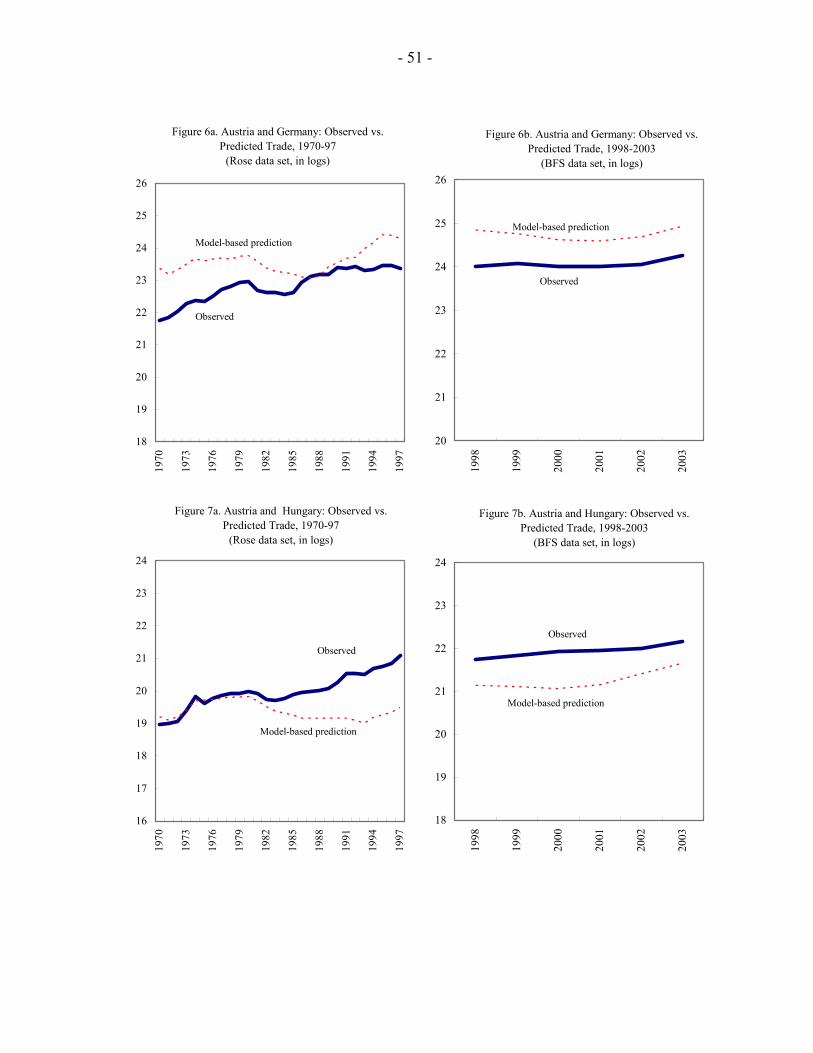
- 51 -
Figure 6a. Austria and Germany: Observed vs. Predicted Trade, 1970-97
(Rose data set, in logs)
18
19
20
21
22
23
24
25
26
1970
1973
1976
1979
1982
1985
1988
1991
1994
1997
Model-based prediction
Observed
Figure 6b. Austria and Germany: Observed vs. Predicted Trade, 1998-2003
(BFS data set, in logs)
20
21
22
23
24
25
26
1998
1999
2000
2001
2002
2003
Model-based prediction
Observed
Figure 7a. Austria and Hungary: Observed vs. Predicted Trade, 1970-97
(Rose data set, in logs)
16
17
18
19
20
21
22
23
24
1970
1973
1976
1979
1982
1985
1988
1991
1994
1997
Model-based prediction
Observed
Figure 7b. Austria and Hungary: Observed vs. Predicted Trade, 1998-2003
(BFS data set, in logs)
18
19
20
21
22
23
24
1998
1999
2000
2001
2002
2003
Observed
Model-based prediction
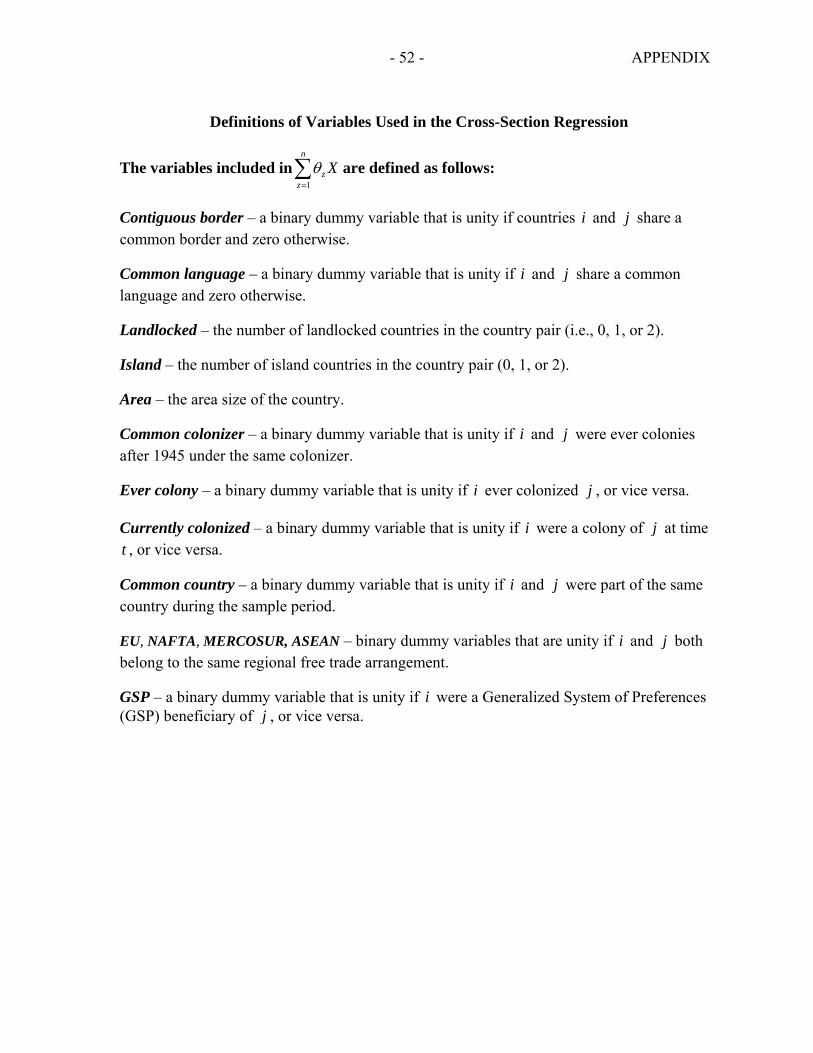
- 52 - APPENDIX
Definitions of Variables Used in the Cross-Section Regression
The variables included in1
n
zz
Xθ=∑ are defined as follows:
Contiguous border – a binary dummy variable that is unity if countries i and j share a common border and zero otherwise.
Common language – a binary dummy variable that is unity if i and j share a common language and zero otherwise.
Landlocked – the number of landlocked countries in the country pair (i.e., 0, 1, or 2).
Island – the number of island countries in the country pair (0, 1, or 2).
Area – the area size of the country.
Common colonizer – a binary dummy variable that is unity if i and j were ever colonies after 1945 under the same colonizer.
Ever colony – a binary dummy variable that is unity if i ever colonized j , or vice versa.
Currently colonized – a binary dummy variable that is unity if i were a colony of j at time t , or vice versa.
Common country – a binary dummy variable that is unity if i and j were part of the same country during the sample period.
EU, NAFTA, MERCOSUR, ASEAN – binary dummy variables that are unity if i and j both belong to the same regional free trade arrangement.
GSP – a binary dummy variable that is unity if i were a Generalized System of Preferences (GSP) beneficiary of j , or vice versa.
- 53 -
References
Arora, Vivek, and Athanasios Vamvakidis, 2005, “How Much Do Trading Partners Matter for Economic Growth?” IMF Staff Papers, Vol. 52 (No. 2 ), pp. 24-40.
Bussière, Matthieu, Jarko Fidrmuc and Bernd Schnatz, 2005, “Trade Integration of the New EU Member States and Selected South-East European countries: Lessons from a Gravity Model,” in European Economic Integration and South-East Europe: Challenges and Prospects, ed. by K. Liebscher and others (Cheltenham, England and Northhampton, Massachusetts; forthcoming).
Cheung, Yin-Wong, and Frank Westermann, 1999, “An Analysis of German Effects on the Austrian Business Cycle,” Weltwirtschaftliches Archiv, Vol. 135 (No. 3), pp. 522-31.
—2000, “Does Austria Respond to the German or the US Business Cycle?” International Journal of Finance and Economics, Vol. 5 (No. 1), pp. 33-42.
Demekas, Dimitri G. and others, 2005, “Foreign Direct Investment in Southeastern Europe: How (and How Much) Can Policies Help?” IMF Working Paper 05/110 (Washington: International Monetary Fund).
Eichengreen, Barry, and Douglas A. Irwin, 1998, “The Role of History in Bilateral Trade Flows,” in The Regionalization of the World Economy, ed. by Jeffrey A. Frankel (Chicago: University of Chicago Press).
Fidrmuc, Jarko, and Iikka Korhonen, 2003, “Similarity of Supply and Demand Shocks Between the Euro Area and the CEECs,” Economic Systems, Vol. 27 (No. 3), pp. 313-34.
Fidrmuc, Jarko, and others, 2002, “EU Enlargement to the East: Effects on the EU-15 in General and on Austria in Particular,” Austrian National Bank, Focus on Transition, 1/2002.
Kose, M. Ayhan, Guy Meredith, and Christopher M. Towe, 2004, “How Has NAFTA Affected the Mexican Economy? Review and Evidence,” IMF Working Paper 04/59 (Washington: International Monetary Fund).
Kose, Ayhan M., Eswar S. Prasad, and Marco E. Terrones, 2003, “Volatility and Comovement in a Globalized World Economy: An Empirical Exploration,” IMF Working Paper 03/246 (Washington: International Monetary Fund).
Rose, Andrew K., 2004, “Do We Really Know That the WTO Increases Trade?” American Economic Review, Vol. 94 (No. 1), pp. 98-114.
Winckler, Georg, 1993, “The Impact of the Economy of the FRG on the Economy of Austria,” in Unequal Partners: A Comparative Analysis of Relations Between Austria and the Federal Republic of Germany and Between Canada and the United States, ed. by H. von Reikhoff and H. Neuhold (Boulder, Colorado: Westview Press).