research papers

Acta Cryst. (2017). D73, 729–737 https://doi.org/10.1107/S205979831700969X 729

Received 22 March 2017

Accepted 1 July 2017

Edited by S. S. Hasnain, University of Liverpool,

England

Keywords: ice rings; macromolecular

crystallography; data processing; data analysis;

X-ray diffraction; data quality; AUSPEX.

Supporting information: this article has

supporting information at journals.iucr.org/d

AUSPEX: a graphical tool for X-ray diffraction dataanalysis

Andrea Thorn,a,b,c* James Parkhurst,b,c Paul Emsley,c Robert A. Nicholls,c

Melanie Vollmar,b Gwyndaf Evansb and Garib N. Murshudovc

aHamburg Centre for Ultrafast Imaging, Universitat Hamburg, Luruper Chaussee 149, 22761 Hamburg, Germany,bDiamond Light Source, Harwell Science and Innovation Campus, Didcot OX11 0DE, England, and cMRC Laboratory of

Molecular Biology, Francis Crick Avenue, Cambridge Biomedical Campus, Cambridge CB2 0QH, England.

*Correspondence e-mail: andrea.thorn@web.de

In this paper, AUSPEX, a new software tool for experimental X-ray data

analysis, is presented. Exploring the behaviour of diffraction intensities and

the associated estimated uncertainties facilitates the discovery of underlying

problems and can help users to improve their data acquisition and processing in

order to obtain better structural models. The program enables users to inspect

the distribution of observed intensities (or amplitudes) against resolution as well

as the associated estimated uncertainties (sigmas). It is demonstrated how

AUSPEX can be used to visually and automatically detect ice-ring artefacts

in integrated X-ray diffraction data. Such artefacts can hamper structure

determination, but may be difficult to identify from the raw diffraction images

produced by modern pixel detectors. The analysis suggests that a significant

portion of the data sets deposited in the PDB contain ice-ring artefacts.

Furthermore, it is demonstrated how other problems in experimental X-ray data

caused, for example, by scaling and data-conversion procedures can be detected

by AUSPEX.

1. Introduction

1.1. Diagnostic tools for the processing and interpretation ofX-ray diffraction data

Diagnostic tools are important in all stages of data model-

ling and data analysis as they provide information about the

quality of the data and the model, as well as their relationship

to one another. In crystal structure determination, diffraction

data are interpreted using an atomic model of the unit-cell

content of the crystal and its lattice symmetry. Consequently,

diagnostic tools are important to derive reliable atomic

models from diffraction data. In particular, graphical tools

provide a fast and convenient representation of data and can

reveal problems which might otherwise go unnoticed. As well

as being valuable for users, they are also important to methods

developers during the design and improvement of algorithms.

However, whilst some of the data-processing software for

macromolecular crystallography produces plots of averaged

reflection intensities against resolution, individual data points

for each reflection are not usually shown. Producing the latter

is well within the capability of modern computer systems and,

as we will demonstrate in this paper, it can reveal artefacts in

the data, such as the presence of so-called ice rings, which may

otherwise be hidden by averaging.

1.2. Ice rings

Ice rings are Debye–Scherrer rings observed at specific

resolutions as a result of X-ray diffraction from a multitude of

ISSN 2059-7983

arbitrarily oriented, typically hexagonal or cubic, ice crystals

(Garman & Owen, 2006). Single-crystal X-ray diffraction

experiments are routinely carried out at cryogenic tempera-

tures and almost all crystalline samples of biological macro-

molecules are grown from aqueous media. As a result, ice

rings are a common occurrence in the diffraction from such

samples.

Cubic (Ic) and hexagonal (Ih) ice exhibit similar interatomic

distances and have similar volumetric mass density, and both

exist at ambient pressure. Hexagonal ice is the more common

of the two forms. Cubic ice can be seen as a metastable form of

hexagonal ice, as it occurs only as nanocrystals and with

hexagonal stacking (Fuentes-Landete et al., 2015). The

theoretical powder diffraction peak profiles of Ih and Ic ice are

shown in Fig. 1.

Ice rings can cause problems in data processing and

modelling. Maximum-likelihood methods, as implemented in,

for example, Phaser (McCoy et al., 2007), SHARP (de La

Fortelle & Bricogne, 1997), REFMAC5 (Murshudov et al.,

1996) and S-SAD (Hendrickson & Teeter, 1981), are widely

used for phasing and refinement in macromolecular crystal-

lography. However, they are particularly sensitive to depar-

tures from the assumptions made about the statistical

distribution of data, which can be caused for example by

outliers, unmodelled observations or incorrect error estimates

(Waterman & Evans, 2010). Ice rings can result in a systematic

bias to the estimated reflection intensities from integration

programs; this reduces the information transferred from the

data to the atomic model, and may in extreme cases even

prevent structure solution.

Three strategies are currently available to address the

problem during data processing.

(i) Resolution ranges contaminated by ice diffraction can be

omitted (see Fig. 2). This requires manual intervention to

determine the presence of an ice ring at a certain resolution

(Kabsch, 2010) and may reduce completeness significantly and

systematically, likely distorting the resulting electron-density

maps.

(ii) All integration programs estimate the background

under a reflection (Leslie, 1999; Kabsch, 2010; Parkhurst et al.,

2016); if the ice ring is broad enough (i.e. it covers the entire

integration box for a reflection) and the background is

modelled by a plane, the background estimation may account

for an ice ring. However, if an ice ring is narrow or irregular

then current background models can fail to account for this

diffraction (see Fig. 3).

(iii) Images can be pre-processed (Chapman & Soma-

sundaram, 2010) to remove the background created by ice

rings. This might not be ideal as it may fail to account for

research papers

730 Thorn et al. � AUSPEX Acta Cryst. (2017). D73, 729–737

Figure 1Theoretical powder diffraction peak profiles for hexagonal ice (Ih) andcubic ice (Ic) at the Cu K� wavelength calculated with XPREP (v.2015/1;Bruker-AXS). For the observed powder diffraction patterns, see Fuentes-Landete et al. (2015).

Figure 2AUSPEX plot of Fobs versus resolution for PDB entry 4puc, the structureof a SusD homologue determined by the Joint Centre for StructuralGenomics; no integration program was given for these deposited data,but scaling was performed with XSCALE (Kabsch, 2010, 2012). Maskingout of the ice rings in integration led to a significant omission of data: theoverall completeness is 78.1%.

detector tilt or directionally dependent variation in the

background.

Because none of these strategies are universally applicable

and result in a complete data set without any ice-ring

contamination, the optimization of cryoconditions (the

conditions under which a crystal is cooled to the desired

temperature) is an important step in macromolecular crys-

tallography (Mitchell & Garman, 1994). Suitable conditions

show diffraction of the macromolecular specimen without ice

diffraction: ice rings are typically detected by the inspection of

X-ray diffraction images, often during cryocondition optimi-

zation (Mitchell & Garman, 1994) or during data collection. In

addition to the inspection of detector images, as early as 1996

McFerrin and Snell proposed the use of resolution-averaged

intensity, then called ‘powder integrated intensity’, as an

indicator of the presence of ice rings.

The need for alternative means of ice-ring detection has

recently been emphasized by the proliferation of pixel

detectors with millisecond readout times. This readout speed

and the low noise in images from such detectors poses an

advantage, and images from such detectors usually cover a

smaller angular increment (‘fine slicing’) than images collected

using earlier detector technologies, leading to shorter expo-

sure times. Consequently, ice rings (and other background-

related problems) are hard to identify by visual inspection of

single images alone. They become more evident if images are

summed together, for example with DIALS (Waterman et al.,

2013), to produce a ‘stacked image’, as shown in Fig. 4.

In the presence of an ice ring, the calculated structure-factor

amplitudes Fcalc and observed structure-factor amplitudes Fobs

(derived from peak integration of the X-ray image) diverge

noticeably. Therefore, ice rings

are also visible as outliers in plots

of the crystallographic R value or

similar indicators against resolu-

tion.

However, after data integra-

tion and scaling, and before

structure solution, ice rings are

more difficult to identify because

two-dimensional information

from the diffraction image has

been reduced by data integration

and a structural model is not

yet available for comparison.

After data reduction, only two

currently available programs give

an indication of ice-ring contam-

ination: phenix.xtriage (Zwart et

al., 2005) and CTRUNCATE

(Winn et al., 2011).

In order to address the need

for a more detailed analysis and

representation of data at this

stage, a new software tool,

AUSPEX1, is presented here. It

can be used to detect the

presence of ice rings and analyse X-ray diffraction intensities

and their estimated standard uncertainties after integration

and before a structural model is available.

1.3. Outline of this paper

In this paper, we will first describe how a preliminary study

on data from the Joint Centre for Structural Genomics (JCSG;

Elsliger et al., 2010) led to the development of AUSPEX,

which we then used to evaluate 200 randomly selected struc-

tures from the PDB (Berman et al., 2003). Subsequently, the

automatic ice-ring detection is described and compared with

other methods that are currently available. We then show

examples of how AUSPEX can be used to identify other

features in the data.

For the purposes of this article, Iobs and Fobs relate to the

observed values of intensity and structure-factor amplitude,

respectively, after data integration and scaling.

2. Preliminary study

In a preliminary study, 156 integrated and scaled data sets

from the JCSG measured using PILATUS detectors and

deposited in the PDB between 2011 and 2015 were evaluated

(test set A; see Supporting Information). The observed

amplitudes Fobs were plotted against resolution. In these plots,

ice rings were visibly identifiable in 15 of the 156 data sets (for

an example, see Fig. 3). This indicates that the background

estimation used in processing these data sets was insufficient

research papers

Acta Cryst. (2017). D73, 729–737 Thorn et al. � AUSPEX 731

Figure 3(a) AUSPEX plot of Iobs versus resolution for PDB entry 4epz. This data set was processed with DIALS andscaled with AIMLESS (Evans & Mushudov, 2013). For hexagonal ice there should be nine rings visible atthis resolution (see Fig. 1), while for cubic ice there should be three (at 3.67, 2.25 and 1.92 A). Theresolution ranges corresponding to potential ice rings are marked using grey bars (whether hexagonal orcubic ice). Two ice rings are clearly visible at high resolution, while the other (at least one more must bepresent even for cubic ice at 3.67 A) was successfully modelled in integration. Hence, when identifying icerings in integrated data, the presence of all ice rings in question is not a reliable criterion. (b) Backgroundoverestimation and underestimation: this enlarged view of the ice ring at 1.918 A shows the effects ofinsufficient background correction. The blue line shows the likely background as assumed by theintegration program (DIALS). The yellow line shows the likely background caused by ice. The discrepancycauses an underestimation of Iobs values to the left and right of the ice ring, resulting in large negativeintensity values, and an overestimation of Iobs in the ice ring, resulting in a peak in Iobs values.

1 Auspex. Latin: diviner; augur; a person who observes birds in order toforetell the future.

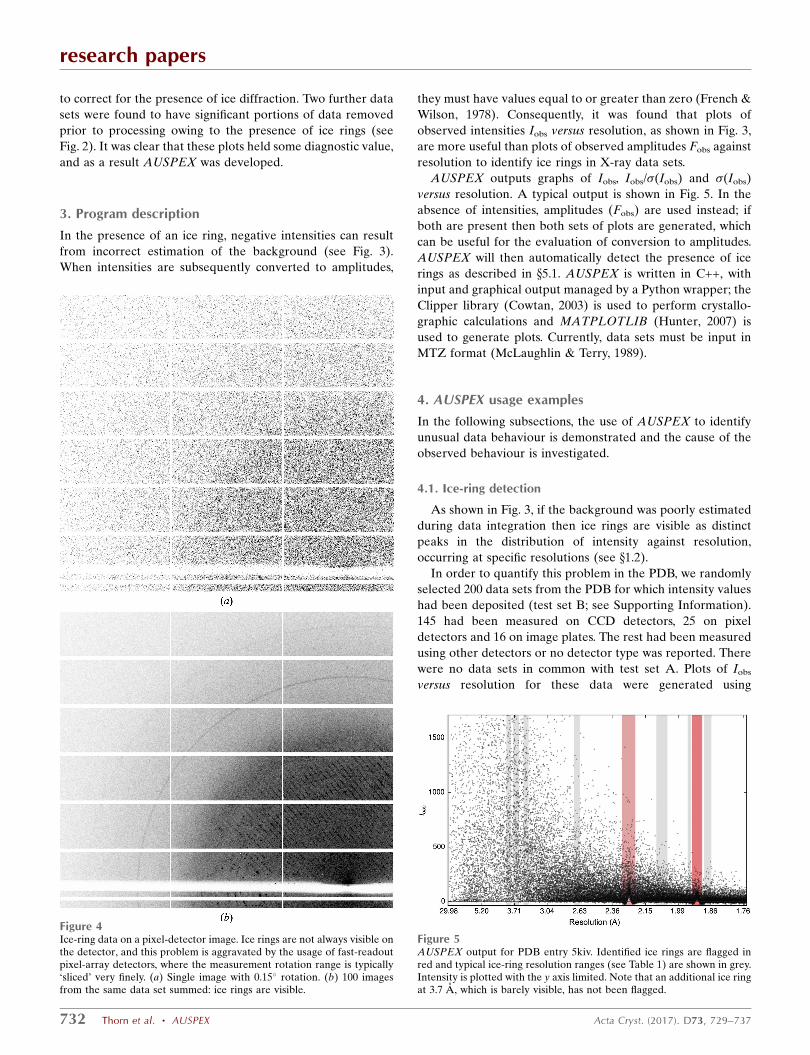
to correct for the presence of ice diffraction. Two further data

sets were found to have significant portions of data removed

prior to processing owing to the presence of ice rings (see

Fig. 2). It was clear that these plots held some diagnostic value,

and as a result AUSPEX was developed.

3. Program description

In the presence of an ice ring, negative intensities can result

from incorrect estimation of the background (see Fig. 3).

When intensities are subsequently converted to amplitudes,

they must have values equal to or greater than zero (French &

Wilson, 1978). Consequently, it was found that plots of

observed intensities Iobs versus resolution, as shown in Fig. 3,

are more useful than plots of observed amplitudes Fobs against

resolution to identify ice rings in X-ray data sets.

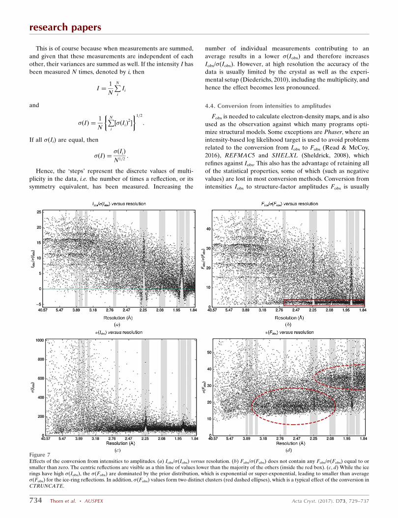
AUSPEX outputs graphs of Iobs, Iobs/�(Iobs) and �(Iobs)

versus resolution. A typical output is shown in Fig. 5. In the

absence of intensities, amplitudes (Fobs) are used instead; if

both are present then both sets of plots are generated, which

can be useful for the evaluation of conversion to amplitudes.

AUSPEX will then automatically detect the presence of ice

rings as described in x5.1. AUSPEX is written in C++, with

input and graphical output managed by a Python wrapper; the

Clipper library (Cowtan, 2003) is used to perform crystallo-

graphic calculations and MATPLOTLIB (Hunter, 2007) is

used to generate plots. Currently, data sets must be input in

MTZ format (McLaughlin & Terry, 1989).

4. AUSPEX usage examples

In the following subsections, the use of AUSPEX to identify

unusual data behaviour is demonstrated and the cause of the

observed behaviour is investigated.

4.1. Ice-ring detection

As shown in Fig. 3, if the background was poorly estimated

during data integration then ice rings are visible as distinct

peaks in the distribution of intensity against resolution,

occurring at specific resolutions (see x1.2).

In order to quantify this problem in the PDB, we randomly

selected 200 data sets from the PDB for which intensity values

had been deposited (test set B; see Supporting Information).

145 had been measured on CCD detectors, 25 on pixel

detectors and 16 on image plates. The rest had been measured

using other detectors or no detector type was reported. There

were no data sets in common with test set A. Plots of Iobs

versus resolution for these data were generated using

research papers

732 Thorn et al. � AUSPEX Acta Cryst. (2017). D73, 729–737

Figure 4Ice-ring data on a pixel-detector image. Ice rings are not always visible onthe detector, and this problem is aggravated by the usage of fast-readoutpixel-array detectors, where the measurement rotation range is typically‘sliced’ very finely. (a) Single image with 0.15� rotation. (b) 100 imagesfrom the same data set summed: ice rings are visible.

Figure 5AUSPEX output for PDB entry 5kiv. Identified ice rings are flagged inred and typical ice-ring resolution ranges (see Table 1) are shown in grey.Intensity is plotted with the y axis limited. Note that an additional ice ringat 3.7 A, which is barely visible, has not been flagged.

AUSPEX and were manually inspected for peak features

similar to those shown in Figs. 2 and 3. Of the 200 data sets,

which were collected between 1995 and 2015, 41 contained ice

rings. (Three additional data sets contained ice rings and part

of the data had been omitted in resolution bins; one data set

had data omitted in resolution bins and no additional ice rings

were visible in the rest of the data.) Inspection of other test

sets from the PDB resulted in similar numbers (see, for

example, x5.2). The high fraction of ice-ring-contaminated

data sets clearly demonstrates the need for better background

estimation and better diagnostic tools to alert users to the

presence of ice rings.

4.2. Ice-ring shift

In five of the 200 cases, ice rings were shifted in resolution

from the typical ice-ring resolution ranges used in AUSPEX

(see Table 1). The five cases in question (PDB entries 1nrj,

5ek4, 3mtl, 3wn2 and 5a30) were tested with the ‘Anomalous

bond length’ feature in the WHAT IF online service (Vriend,

1990), which compares the bond distances in the model with

standard values for protein and nucleic acid bond lengths. All

five cases showed a significant systematic deviation according

to WHAT IF. This, as well as the shift of the ice rings from

their usual resolution ranges, may be caused by an error in the

unit-cell dimensions, which is often the result of the use of an

incorrect X-ray wavelength or detector distance during data

processing (Thorn, 2011).

4.3. Effects of multiplicity on Iobs/r(Iobs) at low resolution

Plots of Iobs/�(Iobs) [and plots of Fobs/�(Fobs)] versus reso-

lution often show clustering around certain values at low

resolution. When considering the associated multiplicity

values (see Fig. 6), it was evident that the higher the multi-

plicity, the larger Iobs/�(Iobs) is.

research papers

Acta Cryst. (2017). D73, 729–737 Thorn et al. � AUSPEX 733

Figure 6Plot of Iobs/�(Iobs) versus resolution for PDB entry 4epz. (a) At high resolution ice rings are clearly visible, while at low resolution the values areclustered, forming a ‘ladder-like’ scatter plot. (b) The same plot coloured by multiplicity. The higher the multiplicity the larger Iobs/�(Iobs) is, thusaccounting for the behaviour. The value of a measurement is less uncertain the more often it has been made, as shown for example by Watkin & Cooper(2016). At low resolution, the main influence on these values is their multiplicity. In contrast, at high resolution weaker reflections are influenced by otherfactors.

Table 1Resolutions used in AUSPEX ice-ring identification; each bin has a startand end value, which have been manually curated.

Bin No. Start (A) End (A)

1 3.953 3.8072 3.753 3.5813 3.482 3.3714 2.692 2.6355 2.294 2.2096 2.094 2.0417 1.954 1.9398 1.935 1.8979 1.890 1.86310 1.723 1.71211 1.527 1.51612 1.476 1.46513 1.446 1.43414 1.372 1.36515 1.305 1.29216 1.285 1.24717 1.240 1.21718 1.186 1.16219 1.136 1.11920 1.099 1.06721 1.052 1.02922 1.017 1.01123 1.000 0.98424 0.981 0.97525 0.973 0.966

This is of course because when measurements are summed,

and given that these measurements are independent of each

other, their variances are summed as well. If the intensity I has

been measured N times, denoted by i, then

I ¼1

N

PNi

Ii

and

�ðIÞ ¼1

N

PNi

½�ðIiÞ2�

� �1=2

:

If all �(Ii) are equal, then

�ðIÞ ¼� Iið Þ

N1=2:

Hence, the ‘steps’ represent the discrete values of multi-

plicity in the data, i.e. the number of times a reflection, or its

symmetry equivalent, has been measured. Increasing the

number of individual measurements contributing to an

average results in a lower �(Iobs) and therefore increases

Iobs/�(Iobs). However, at high resolution the accuracy of the

data is usually limited by the crystal as well as the experi-

mental setup (Diederichs, 2010), including the multiplicity, and

hence the effect becomes less pronounced.

4.4. Conversion from intensities to amplitudes

Fobs is needed to calculate electron-density maps, and is also

used as the observation against which many programs opti-

mize structural models. Some exceptions are Phaser, where an

intensity-based log likelihood target is used to avoid problems

related to the conversion from Iobs to Fobs (Read & McCoy,

2016), REFMAC5 and SHELXL (Sheldrick, 2008), which

refines against Iobs. This also has the advantage of retaining all

of the statistical properties, some of which (such as negative

values) are lost in most conversion methods. Conversion from

intensities Iobs to structure-factor amplitudes Fobs is usually

research papers

734 Thorn et al. � AUSPEX Acta Cryst. (2017). D73, 729–737

Figure 7Effects of the conversion from intensities to amplitudes. (a) Iobs/�(Iobs) versus resolution. (b) Fobs/�(Fobs) does not contain any Fobs/�(Fobs) equal to orsmaller than zero. The centric reflections are visible as a thin line of values lower than the majority of the others (inside the red box). (c, d) While the icerings have high �(Iobs), the �(Fobs) are dominated by the prior distribution, which is exponential or super-exponential, leading to smaller than average�(Fobs) for the ice-ring reflections. In addition, �(Fobs) values form two distinct clusters (red dashed ellipses), which is a typical effect of the conversion inCTRUNCATE.

performed using the French and Wilson algorithm (French &

Wilson, 1978), which uses a Bayesian approach prior that

forces negative Fobs values to be positive or zero-valued and

Wilson-distributed. This prior may not be appropriate if the

data are contaminated by ice rings (see x4.1) or if other

systematic errors are present. The changes introduced by the

conversion, as implemented for example in CTRUNCATE,

can be illustrated by comparing AUSPEX plots of Iobs/�(Iobs)

with Fobs/�(Fobs) (see Fig. 7).

5. Automatic ice-ring detection

5.1. Implementation in AUSPEX

The automatic ice-ring detection procedure considers the

behaviour of the standardized mean hIobsi/s in resolution bins,

where hIobsi is the sample mean and s is the sample standard

deviation of the intensities in a given bin. By default, equally

spaced inverse-resolution bins of 0.001 A�1 are used so as to

achieve a reasonable compromise between binning fineness

and noise.

Since data may contain various peculiarities, either inherent

to the data or as a consequence of data processing, the

observed average standardized mean hIobsi/s may be system-

atically higher or lower than the theo-

retical value and may be correlated with

the resolution. In order to be able to

detect and analyse ice rings, which only

occur within certain resolution ranges

(see Table 1), it is useful to ‘remove’ the

effect of such behaviour. To perform

this, the local average standardized

mean is estimated as a function of

resolution and compared with the

observed standardized mean in a given

bin. In the current implementation, this

resolution-dependent function f is

calculated by performing interquartile-

range filtering and robust Gaussian

smoothing on the standardized mean

after excluding the potential ice-ring

ranges. Interpolation then allows esti-

mates of the standardized mean to be

achieved for each bin located within the

potential ice-ring ranges.

For each bin, an ice-detection score is

then calculated, S = N1/2(hIobsis�1� f),

where the factor N1/2 accounts for

differences in the number of observa-

tions per bin, thus stabilizing the score

across all resolution ranges. This score

essentially measures the departure from

the typical shape of the intensity distri-

bution in the given data set, and can be

loosely interpreted as a Z-score. This is

sensitive to resolution ranges that

exhibit sudden sharp changes in the

intensity distribution, thus facilitating the detection and

assessment of ice rings.

Owing to poor background estimation, the presence of ice

rings can cause an increase or decrease in the mean intensity

hIobsi (see Fig. 3) but not in the standard deviation of the

intensity distribution. Consequently, the standardized mean

and therefore S should increase or decrease in the presence of

ice rings. However, the standard deviation can be increased or

decreased relative to the mean by other problems in data

processing, resulting in a particularly low score. Consequently,

both positive and negative extreme score outliers are identi-

fied and flagged red in the plots (the default outlier threshold

is �5), as shown in Fig. 5, which shows a typical output. In

Fig. 8, the ice-detection score S = N1/2(hIobsis�1� f) is shown

together with the plot of Iobs against resolution for PDB entry

3jqy.

5.2. Comparison to other programs

We selected another test set of 200 random data sets from

the PDB for which intensity values had been deposited (test

set C; see Supporting Information). By visual inspection of the

AUSPEX plots, 45 of these contained ice rings, some of which

research papers

Acta Cryst. (2017). D73, 729–737 Thorn et al. � AUSPEX 735

Figure 8Automatic detection of ice rings in AUSPEX for PDB entry 3jqy. (a) Plot of the ice-detection score[‘Icefinder score’, black line; S = N1/2(hIobsis

�1� f )] against resolution. The threshold of �5 is

marked by horizontal red lines. (b) Plot of Iobs against resolution with potential ice-ring resolutionranges in grey and flagged resolution ranges in red. The ice rings are clearly visible in both plots.

were very weak. This was a similar fraction as found

previously by visual inspection of test set B.

Of these 45 structures, six had missing data owing to the

omission of entire resolution shells from the data.

Each of the 200 structures was analysed with AUSPEX,

CTRUNCATE and phenix.xtriage; the results are shown in

Table 2. CTRUNCATE gives a large number of false positives;

phenix.xtriage applies more rigid criteria, resulting in fewer

false positives but also more false negatives. AUSPEX

performs more consistently in the four categories of false/

correct positives and false/correct negatives. The AUSPEX

implementation of automatic ice-ring detection is still inferior

to the visual inspection of AUSPEX plots.

5.3. Testing of the algorithm against a large number of datasets

Using this method, a large part of the PDB was evaluated.

We found that 19% (5438 out of 28 895) of data sets with

intensities deposited were suspected to have contamination

owing to ice. This percentage is in keeping with the results

from our more limited visual inspection of intensity versus

resolution plots. This is a significant fraction which remains

relatively consistent even in recent depositions in the PDB,

demonstrating that this pathology is generally overlooked,

presumably owing to a lack of necessary diagnostics, and that

more sophisticated background-determination algorithms are

needed to improve intensity estimation.

5.4. Limitations

AUSPEX identifies all resolution ranges where ice rings are

typically observed for hexagonal or cubic ice (see Table 1)

with an associated score S outside a given threshold range (the

default is �5).

AUSPEX will not identify Debye–Scherrer rings from

sources other than ice. Such rings can be caused, for example,

by the crystallization plates used in in situ screening or by

sample holders. Since AUSPEX only searches for ice rings in

the expected resolution ranges (Table 1), it also cannot

automatically detect ice rings if the wavelength or detector

distance employed in data processing are wrong. However,

AUSPEX could be extended in future to allow the detection

of other phenomena such as rings caused by detergents and

lipids, as used for example in membrane-protein crystal-

lization.

If there is any doubt over the presence of an ice ring, the

plot of the intensity distribution against resolution output by

AUSPEX should be examined (see above).

6. Conclusion

Even after more than 20 years of specific research to minimize

the influence of ice diffraction in macromolecular crystallo-

graphy (Mitchell & Garman, 1994), ice-ring artefacts were

present in roughly 20% of 400 data sets (test sets B and C)

chosen randomly from the PDB (as found by visual inspection

of plots of Iobs versus resolution). A similar percentage (19%)

was obtained when 28 895 data sets from the PDB for which

intensities had been deposited were evaluated with the auto-

matic ice-ring detection implemented in AUSPEX.

Optimization of cryoconditions so as to avoid ice rings is

hampered by the difficulty in recognizing their presence on

diffraction images, in particular images from modern pixel-

array detectors, or from scaling statistics. In order to address

this problem, a new software tool, AUSPEX, has been

developed to facilitate ice-ring detection, allowing visual

inspection of the intensity (or amplitude) distribution versus

resolution as well as automatic ice-ring detection. The auto-

matic ice-ring detection is arguably an improvement over

current methods, although visual inspection of AUSPEX plots

is presently the most reliable detection method.

The program can be used after scaling to check for data

pathology, helping the user to decide whether it is necessary to

re-integrate and rescale. It is also useful when looking at data

sets that have already been solved in order to check the

quality of the data underlying a model.

AUSPEX can also be used to investigate the structure and

the distribution of errors within crystallographic data sets. The

examples given illustrate effects associated with the multi-

plicity of measurements as well as the conversion from

intensities to amplitudes. Although there is little direct

evidence to suggest that these effects have a negative influence

on structure solution using current software programs, there is

clearly scope to improve the estimation of measurement errors

in diffraction data (Waterman & Evans, 2010).

Furthermore, AUSPEX has inspired the development of an

improved approach to background estimation that has been

implemented in DIALS (Parkhurst et al., 2017).

The program will be released in the near future as part of

CCP4 (Winn et al., 2011).

Acknowledgements

The authors would like to thank Christian Thorn, Harry

Powell, Phil Evans, David Watkin, Richard Cooper, Charles

Ballard, Armin Wagner and Daniel Bowron for discussions,

and Jake Grimmett and Toby Darling from the MRC

Laboratory of Molecular Biology for computing support.

research papers

736 Thorn et al. � AUSPEX Acta Cryst. (2017). D73, 729–737

Table 2Results of automatic ice-ring detection in phenix.xtriage (Zwart et al.,2005) and CTRUNCATE (Winn et al., 2011) for 200 cases randomlyselected from the PDB, as described in x5.2.

There were 42 data sets that contained ice rings (see test set C in theSupporting Information). Six cases where data at ice-ring resolutions had beenomitted were included in this test set. phenix.xtriage gives a message if onlyone ice ring has been found instead of an ice-ring warning; for the purposes ofthis test these messages were treated as ‘positives’.

Correctpositives

Correctnegatives

Falsepositives

Falsenegatives

phenix.xtriage 14/42 145/158 13 28CTRUNCATE 23/42 88/158 70 19AUSPEX 25/42 143/158 14 17

Funding information

This work was supported by the European Union FP7 Marie-

Curie IEF grant SOUPINMYCRYSTAL (AT), by BiostructX

(project No. 283570 of the European Union FP7 framework)

(JP), by CCP4/STFC grant No. PR140014 (RN) and by MRC

grant No. MC_UP_A025_1012 (GNM and PE).

References

Berman, H. M., Henrick, K. & Nakamura, H. (2003). Nature Struct.Biol. 10, 980.

Chapman, M. S. & Somasundaram, T. (2010). Acta Cryst. D66,741–744.

Cowtan, K. (2003). IUCr Comput. Commun. Newsl. 2, 4–9.Diederichs, K. (2010). Acta Cryst. D66, 733–740.Elsliger, M.-A., Deacon, A. M., Godzik, A., Lesley, S. A., Wooley, J.,

Wuthrich, K. & Wilson, I. A. (2010). Acta Cryst. F66, 1137–1142.Evans, P. R. & Murshudov, G. N. (2013). Acta Cryst. D69, 1204–1214.French, S. & Wilson, K. (1978). Acta Cryst. A34, 517–525.Fuentes-Landete, V., Mitterdorfer, C., Handle, P. H., Ruiz, G. N.,

Bernard, J., Bogdan, A., Seidl, M., Amann-Winkel, K., Stern, J.,Fuhrmann, S. & Loerting, T. (2015). Water: Fundamentals as theBasis for Understanding the Environment and Promoting Tech-nology, edited by P. G. Debenedetti, M. A. Ricci & F. Bruni, p. 178,Fig. 2. Amsterdam: IOS Press.

Garman, E. F. & Owen, R. L. (2006). Acta Cryst. D62, 32–47.Hendrickson, W. A. & Teeter, M. M. (1981). Nature (London), 290,

107–113.Hunter, J. D. (2007). Comput. Sci. Eng. 9, 90–95.Kabsch, W. (2010). Acta Cryst. D66, 133–144.Kabsch, W. (2012). International Tables for Crystallography, Vol. F,

2nd online ed., edited by E. Arnold, D. M. Himmel & M. G.

Rossmann, pp. 272–281. Chester: International Union of Crystallo-graphy.

La Fortelle, E. de & Bricogne, G. (1997). Methods Enzymol. 276,472–494.

Leslie, A. G. W. (1999). Acta Cryst. D55, 1696–1702.McCoy, A. J., Grosse-Kunstleve, R. W., Adams, P. D., Winn, M. D.,

Storoni, L. C. & Read, R. J. (2007). J. Appl. Cryst. 40, 658–674.McLaughlin, S. & Terry, H. (1989). MTZLIB. http://www.ccp4.ac.uk/

html/mtzlib.html.Mitchell, E. P. & Garman, E. F. (1994). J. Appl. Cryst. 27, 1070–1074.Murshudov, G., Vagin, A. & Dodson, E. (1996). Proceedings of the

CCP4 Study Weekend. Macromolecular Refinement, edited by E.Dodson, M. Moore, A. Ralph & S. Bailey, pp. 93–104. Warrington:Daresbury Laboratory.

Parkhurst, J. M., Thorn, A., Vollmar, M., Winter, G., Waterman, D. G.,Gildea, R. J., Fuentes-Montero, L., Murshudov, G. N. & Evans, G.(2017). IUCrJ, 4, 626–638.

Parkhurst, J. M., Winter, G., Waterman, D. G., Fuentes-Montero, L.,Gildea, R. J., Murshudov, G. N. & Evans, G. (2016). J. Appl. Cryst.49, 1912–1921.

Read, R. J. & McCoy, A. J. (2016). Acta Cryst. D72, 375–387.Sheldrick, G. M. (2008). Acta Cryst. A64, 112–122.Thorn, A. (2011). PhD thesis, p. 28. Georg-August-Universitat

Gottingen, Germany. http://hdl.handle.net/11858/00-1735-0000-0006-B072-8.

Vriend, G. (1990). J. Mol. Graph. 8, 52–56.Waterman, D. & Evans, G. (2010). J. Appl. Cryst. 43, 1356–1371.Waterman, D. G., Winter, G., Parkhurst, J. M., Fuentes-Montero, L.,

Hattne, J., Brewster, A., Sauter, N. K. & Evans, G. (2013). CCP4Newsl. Protein Crystallogr. 49, 16–19.

Watkin, D. J. & Cooper, R. I. (2016). Acta Cryst. B72, 661–683.Winn, M. D. et al. (2011). Acta Cryst. D67, 235–242.Zwart, P. H., Grosse-Kunstleve, R. W. & Adams, P. D. (2005). CCP4

Newsl. Protein Crystallogr. 43, contribution 7.

research papers

Acta Cryst. (2017). D73, 729–737 Thorn et al. � AUSPEX 737