Embed Size (px)
Citation preview
AusNet Electricity Services Pty Ltd
Electricity Distribution Price Review 2016–20
Appendix 4B: Demand Forecasting Methodology
Submitted: 30 April 2015

Demand Forecasting Methodology
Electricity Distribution Network
Document number AMS 20-30
Issue number 1.2
Status Final
Approver Nick Cimdins
Date of approval 20/04/2015

AusNet Services AMS 20-30
Demand Forecasting Methodology – Electricity Distribution Network
ISSUE 1.2 20/04/2015 2 / 34
UNCONTROLLED WHEN PRINTED
ISSUE/AMENDMENT STATUS
Issue Number
Date Description Author Approved
by
1 03/08/2011 Creation H de Beer
L Russell
D Postlethwaite
A Parker
1.1 03/07/2014 Updated for new process L Russell N Cimdins
1.2 20/04/2015 Minor revisions L Russell N Cimdins
Disclaimer
This template is for generating internal and external document belonging to AusNet Services and may or may not contain all available information on the subject matter this document purports to address.
The information contained in this document is subject to review and AusNet Services may amend this document at any time. Amendments will be indicated in the Amendment Table, but AusNet Services does not undertake to keep this document up to date.
To the maximum extent permitted by law, AusNet Services makes no representation or warranty (express or implied) as to the accuracy, reliability, or completeness of the information contained in this document, or its suitability for any intended purpose. AusNet Services (which, for the purposes of this disclaimer, includes all of its related bodies corporate, its officers, employees, contractors, agents and consultants, and those of its related bodies corporate) shall have no liability for any loss or damage (be it direct or indirect, including liability by reason of negligence or negligent misstatement) for any statements, opinions, information or matter (expressed or implied) arising out of, contained in, or derived from, or for any omissions from, the information in this document.
Contact
This document is the responsibility of Regulation and Network Strategy, Asset Management, AusNet Services. Please contact the indicated owner of the document with any inquiries.
Luke Russell
AusNet Services
Level 31, 2 Southbank Boulevard
Melbourne Victoria 3006
Ph: (03) 9695 6539
AusNet Services AMS 20-30
Demand Forecasting Methodology – Electricity Distribution Network
ISSUE 1.2 20/04/2015 3 / 34
UNCONTROLLED WHEN PRINTED
Table of Contents
1 Executive Summary ..................................................................................................................... 5
1.1 Obligations ................................................................................................................................................... 5
1.2 Use ............................................................................................................................................................... 5
1.3 Forecasting Process ................................................................................................................................... 5
2 Purpose ......................................................................................................................................... 6
3 Obligations ................................................................................................................................... 6
4 Use of Forecasts .......................................................................................................................... 7
4.1 Network Planning ........................................................................................................................................ 7
4.2 Other Uses .................................................................................................................................................. 7
5 Outputs.......................................................................................................................................... 8
5.1 Public ........................................................................................................................................................... 8
5.2 AusNet Services .......................................................................................................................................... 8
6 Demand Forecasts ....................................................................................................................... 8
6.1 Overview ...................................................................................................................................................... 8
6.2 Process Summary....................................................................................................................................... 9
7 Detailed Process ........................................................................................................................ 11
7.1 Extract Historical Customer Numbers ...................................................................................................... 11
7.2 Create Sigmoidal Customer Forecasts .................................................................................................... 11
7.3 Adjust Customer Forecasts ...................................................................................................................... 17
7.4 Extract Historical Demand Data ............................................................................................................... 17
7.5 Extract ambient Temperature Data .......................................................................................................... 17
7.6 Customer Normalise Historic Data ........................................................................................................... 17
7.7 S-Curve Analysis of Historical Demand and Ambient Temperature ...................................................... 19
7.8 Demand Efficiency .................................................................................................................................... 19
7.9 P50 and P10 Demand .............................................................................................................................. 20
7.10 Generate Forecast .................................................................................................................................... 20
7.11 Validate Forecast ...................................................................................................................................... 21
8 Forecast Outputs ....................................................................................................................... 22
8.1 Draft Forecasts .......................................................................................................................................... 22
8.2 Endorsed Forecasts .................................................................................................................................. 22
8.3 Archiving .................................................................................................................................................... 22
9 Future Work ................................................................................................................................ 23
10 Notes ........................................................................................................................................... 24
10.1 Unit of Measurement................................................................................................................................. 24
11 Appendix ..................................................................................................................................... 25
11.1 Electricity Distribution Code ...................................................................................................................... 25

AusNet Services AMS 20-30
Demand Forecasting Methodology – Electricity Distribution Network
ISSUE 1.2 20/04/2015 4 / 34
UNCONTROLLED WHEN PRINTED
11.2 Electricity Distribution Price Reset 2011-2015 ........................................................................................ 25
11.3 Historic Analysis ........................................................................................................................................ 26
11.4 Summer Preparedness Process Review................................................................................................. 32

AusNet Services AMS 20-30
Demand Forecasting Methodology – Electricity Distribution Network
ISSUE 1.2 20/04/2015 5 / 34
UNCONTROLLED WHEN PRINTED
1 Executive Summary
This document describes the process by which AusNet Services forecasts the spatial demand which connected customers will place on its electricity distribution network. This forecasting process will produce best practice maximum demand forecasts featuring:
• Accuracy and a lack of bias;
• Transparency and repeatability;
• Incorporation of key drivers; and
• Validation and testing.
1.1 Obligations
The Electricity Distribution Code requires distributors to submit annual plans detailing how the predicted demand for electricity will be supplied at transmission network connection points, at zone substations and high voltage lines in the distribution network. These plans must contain historical demand and forecasts of demand.
The National Electricity Rules require a distribution network service provider to submit operating and capital expenditure forecasts necessary to meet or manage the expected demand for standard control services.
1.2 Use
AusNet Services’ annual load demand forecasts are the starting point for network planning studies which quantify the need for network augmentation to maintain the quality, reliability and security of supplies and to meet or manage the expected demand for service and to prepare contingency plans.
The Australian Energy Regulator uses load demand forecasts to assess and define the future revenue requirements for distributors to meet the expected demand for service from connected customers. Load demand forecasts are also used in the annual development of distribution loss factors to enable an equitable allocation of network operating costs to connected customers.
1.3 Forecasting Process
The eight fundamental steps in the current forecasting process are:
• Validate network configuration;
• Extract historical demand data;
• Validate historical demand data;
• Extract ambient temperature data;
• Correlate historical demand and ambient temperature;
• Regression analysis of historical demand and ambient temperature;
• Generate spatial forecasts; and
• Validate spatial forecasts.

AusNet Services AMS 20-30
Demand Forecasting Methodology – Electricity Distribution Network
ISSUE 1.2 20/04/2015 6 / 34
UNCONTROLLED WHEN PRINTED
2 Purpose
This document describes the process by which AusNet Services forecasts the spatial demand which connected customers will place on its electricity distribution network for the purposes of:
• Ensuring service standards are maintained;
• Planning augmentations to the distribution network;
• Planning augmentations to connections to the Victorian electricity transmission network; and
• Assisting planning of the national electricity transmission network.
3 Obligations
The Electricity Distribution Code1 requires distributors such as AusNet Electricity Services Pty Ltd to submit an
annual plan detailing how the predicted demand for electricity will be supplied:
• At transmission network connection points where the distribution network connects to the declared shared transmission network. This plan must contain historical and forecast demand for the following ten calendar years compared with the capacity of each transmission connection.
• By its distribution network, including subtransmission lines, zone substations and high voltage lines over the following five calendar years. This plan must contain historical and forecast demand compared with the capacity of each zone substation, an assessment of the impact of loss of load for each subtransmission line and zone substation and a description of feasible options for meeting forecast demand including opportunities for embedded generation and demand management.
The National Electricity Rules2 require a distribution network service provider such as AusNet Electricity
Services Pty Ltd to submit an operating expenditure forecast and a capital expenditure forecast for the relevant regulatory control period which is required to:
• meet or manage the expected demand for standard control services;
• comply with regulatory obligations or requirements associated with standard control services;
• maintain the quality, reliability and security of supply of standard control services; and
• maintain the reliability, safety and security of the distribution system.
1 Electricity Distribution Code, Essential Services Commission Victoria.
2 National Electricity Rules, Australian Energy Market Commission.
AusNet Services AMS 20-30
Demand Forecasting Methodology – Electricity Distribution Network
ISSUE 1.2 20/04/2015 7 / 34
UNCONTROLLED WHEN PRINTED
4 Use of Forecasts
4.1 Network Planning
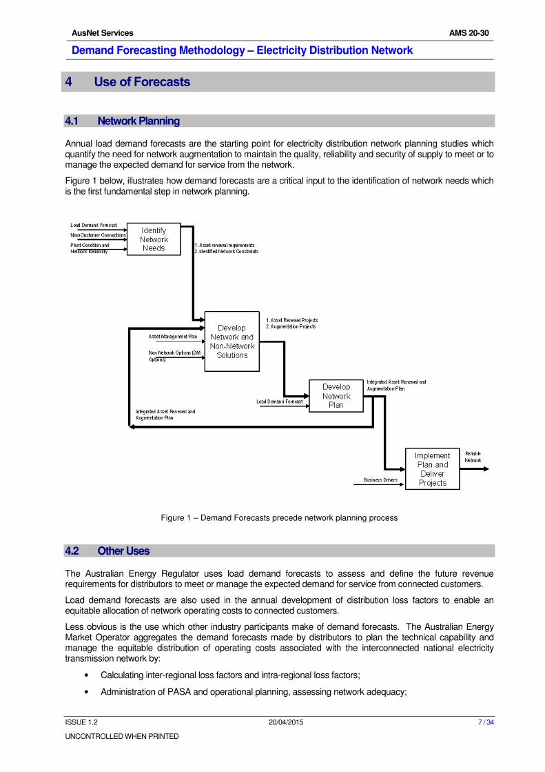
Annual load demand forecasts are the starting point for electricity distribution network planning studies which quantify the need for network augmentation to maintain the quality, reliability and security of supply to meet or to manage the expected demand for service from the network.
Figure 1 below, illustrates how demand forecasts are a critical input to the identification of network needs which is the first fundamental step in network planning.
Figure 1 – Demand Forecasts precede network planning process
4.2 Other Uses
The Australian Energy Regulator uses load demand forecasts to assess and define the future revenue requirements for distributors to meet or manage the expected demand for service from connected customers.
Load demand forecasts are also used in the annual development of distribution loss factors to enable an equitable allocation of network operating costs to connected customers.
Less obvious is the use which other industry participants make of demand forecasts. The Australian Energy Market Operator aggregates the demand forecasts made by distributors to plan the technical capability and manage the equitable distribution of operating costs associated with the interconnected national electricity transmission network by:
• Calculating inter-regional loss factors and intra-regional loss factors;
• Administration of PASA and operational planning, assessing network adequacy;
AusNet Services AMS 20-30
Demand Forecasting Methodology – Electricity Distribution Network
ISSUE 1.2 20/04/2015 8 / 34
UNCONTROLLED WHEN PRINTED
• Central generation dispatch;
• Statement of Opportunities;
• National Transmission Development Plan and the Victorian Annual Planning Report;
• Regulatory Investment Tests;
• Demand Side Management;
• Power Factor obligations under automatic access standard;
• Load shedding facilities; and
• Demand management incentive schemes.
5 Outputs
5.1 Public
Each distributor is required to prepare demand forecasts for each Victorian electricity transmission network connection point (terminal station) and to submit them to the Australian Energy Market Operator by 30 June each year.
Each distributor is required to publish by 30 December each year demand forecasts for each Victorian electricity transmission network connection point (terminal station) in the Transmission Connection Planning Report.
Each distributor is required to publish by 30 December each year demand forecasts for each subtransmission line, zone substation and medium voltage feeder in its distribution network in the Distribution Annual planning Report.
5.2 AusNet Services
In addition to the public forecasts listed in the preceding section, AusNet Services generates the following forecasts to meet specific internal network planning needs:
• In May of each year, forecasts of the peak demand (measured in ampere) are generated for each feeder to facilitate the contingency planning associated with Summer Preparedness works.
• In July each year, forecasts of the peak demand (measured in MVA) are generated for each feeder and zone substation to facilitate network planning for network augmentation works.
6 Demand Forecasts
6.1 Overview
Ten-Year demand forecasts are prepared for terminal stations, zone substations and 22kV feeders each year. They are prepared for 10% Probability of Exceedence (POE) and 50% POE to reflect the temperature sensitivity of load demand. The following inputs are incorporated:
• Load demand growth information of future economic trends in the relevant area, including information from government agencies regarding identified growth areas and long term development plans;
• Actual maximum demands for the most recent 12 months;
• Daily maximum demands for the past 3 to 5 years for the summer and winter periods are weather normalised for establish relationship between demand and temperature;
AusNet Services AMS 20-30
Demand Forecasting Methodology – Electricity Distribution Network
ISSUE 1.2 20/04/2015 9 / 34
UNCONTROLLED WHEN PRINTED
• Recent load growth trends over the previous 5 year period;
• Any known specific new loads expected on the network; and
• Any planned transfers of load to or from other zone substations.
The load demand forecasts provide recorded maximum demands for each of the previous five summers and winters and include a megawatt (MW) and Megavolt amp reactive (MVAr) forecast for each summer and winter period for the next 10 years. The proposed granularity of future forecasts includes:
• Customer;
• Distribution Transformer;
• Load Section;
• Feeder Forecasts;
• Zone Substation Busbar Forecasts;
• Zone Substation Transformer Forecasts;
• Zone Substation Forecasts;
• Terminal Station Busbar Forecasts; and
• Terminal Station Forecasts.
6.2 Process Summary
The fundamental steps in the current spatial and trend analysis forecasting process are:
• Extract historical customer numbers;
• Create sigmoidal customer forecasts;
• Adjust customer forecasts to Victorian Department of Planning forecasts;
• Extract historical demand data;
• Extract ambient temperature data;
• Correlate historical demand and ambient temperature;
• Sigmoidal analysis of historic demand and temperature;
• Generate spatial demand forecasts; and
• Validate spatial demand forecasts.
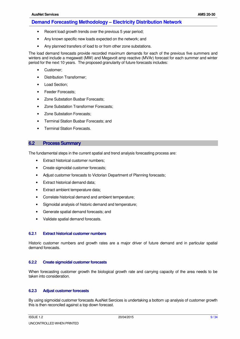
6.2.1 Extract historical customer numbers
Historic customer numbers and growth rates are a major driver of future demand and in particular spatial demand forecasts.
6.2.2 Create sigmoidal customer forecasts
When forecasting customer growth the biological growth rate and carrying capacity of the area needs to be taken into consideration.
6.2.3 Adjust customer forecasts
By using sigmoidal customer forecasts AusNet Sercices is undertaking a bottom up analysis of customer growth this is then reconciled against a top down forecast.

AusNet Services AMS 20-30
Demand Forecasting Methodology – Electricity Distribution Network
ISSUE 1.2 20/04/2015 10 / 34
UNCONTROLLED WHEN PRINTED
6.2.4 Extract historical demand data
OSIpi contains the historic demand data for the network. A series of customisable tools have been created for the extraction of data. These tools are updated with the current network configuration, to include new feeders and zone substations, prior to commencing the data extraction.
6.2.5 Extract ambient temperature data
Ambient temperature data relevant to each feeder and zone substation is also extracted from OSIpi and historic BOM data in a similar manner to the extract process for demand data. Data extraction and validation is under the direction of the forecasting process leader.
6.2.6 Correlate historical demand and ambient temperature
Correlation of demand data against relevant ambient temperature enables the first stage of data filtering to occur. Correlation and identification of incidences of extreme variance is under the direction of the forecasting process leader.
6.2.7 Sigmoidal analysis of historic demand and temperature
Sigmoidal analysis provides a mathematical correlation between demand and ambient temperature.
6.2.8 Generate spatial demand forecasts
Forecasts are generated using the provided tools. These are automated tools that have been programmed with the discussed methodologies and techniques. Historically forecasts were conducted individually for each feeder or zone sub and some individual judgement from the forecaster was applied. In contrast the forecast tools apply a common methodology for all levels of forecasts. Where a forecast is found to be inconsistent any change to correct a single forecast will apply across all forecasts and all levels of forecasts, this ensures consistent forecasts are applied at all times. This is the responsibility of the forecasting process leader.
6.2.9 Validate spatial demand forecasts
Regional network planning engineers in conjunction with the subtransmission planning engineer and the transmission planning engineer validate the relevant forecasts. Validation involves magnitude checks and trend line checks informed by knowledge of the loadings and network configuration changes recently completed and pending.
AusNet Services AMS 20-30
Demand Forecasting Methodology – Electricity Distribution Network
ISSUE 1.2 20/04/2015 11 / 34
UNCONTROLLED WHEN PRINTED
7 Detailed Process
7.1 Extract Historical Customer Numbers
Historical customer numbers are extracted from a MSSQL database; this database captures a snap shot each month of each customer, their attributes such as postcode, etc, and their network status. A set of extracts are create one is for the feeder that each customer was connected to at the time, this provides us with the ability to customer normalise demand and understand where customer are moved from feeder to feeder during this period. The other is for the last feeder they are connected to this provides us with a normalised customer number that removes step changes due to network reconfigurations.
7.2 Create Sigmoidal Customer Forecasts
Customer forecasting is a complex problem, historically straight-line forecasting was used however this has two major drawbacks, the first is under forecasting in areas that are starting to boom due to subdivisions or in new developments, the second is over forecasting areas that have previously boomed where growth rates are decreasing.
AusNet Services uses a sigmoidal forecasting methodology to reduce these flaws. Sigmoidal forecasting is used as the sigmoidal function maps the growth rates seen in all biological systems; they start with slow growth, have a high growth period and then growth saturates. This can be seen in the human body, bacteria or world population. The peak is dictated by the carrying capacity of the organism, the total cannot exceed this and the system regulates growth rates for this to occur.
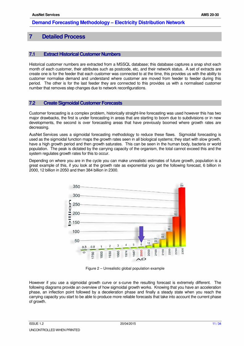
Depending on where you are in the cycle you can make unrealistic estimates of future growth, population is a great example of this, if you look at the growth rate as exponential you get the following forecast, 6 billion in 2000, 12 billion in 2050 and then 384 billion in 2300.
Figure 2 – Unrealistic global population example
However if you use a sigmoidal growth curve or s-curve the resulting forecast is extremely different. The following diagrams provide an overview of how sigmoidal growth works. Knowing that you have an acceleration phase, an inflection point followed by a deceleration phase and finally a steady state when you reach the carrying capacity you start to be able to produce more reliable forecasts that take into account the current phase of growth.
AusNet Services AMS 20-30
Demand Forecasting Methodology – Electricity Distribution Network
ISSUE 1.2 20/04/2015 12 / 34
UNCONTROLLED WHEN PRINTED
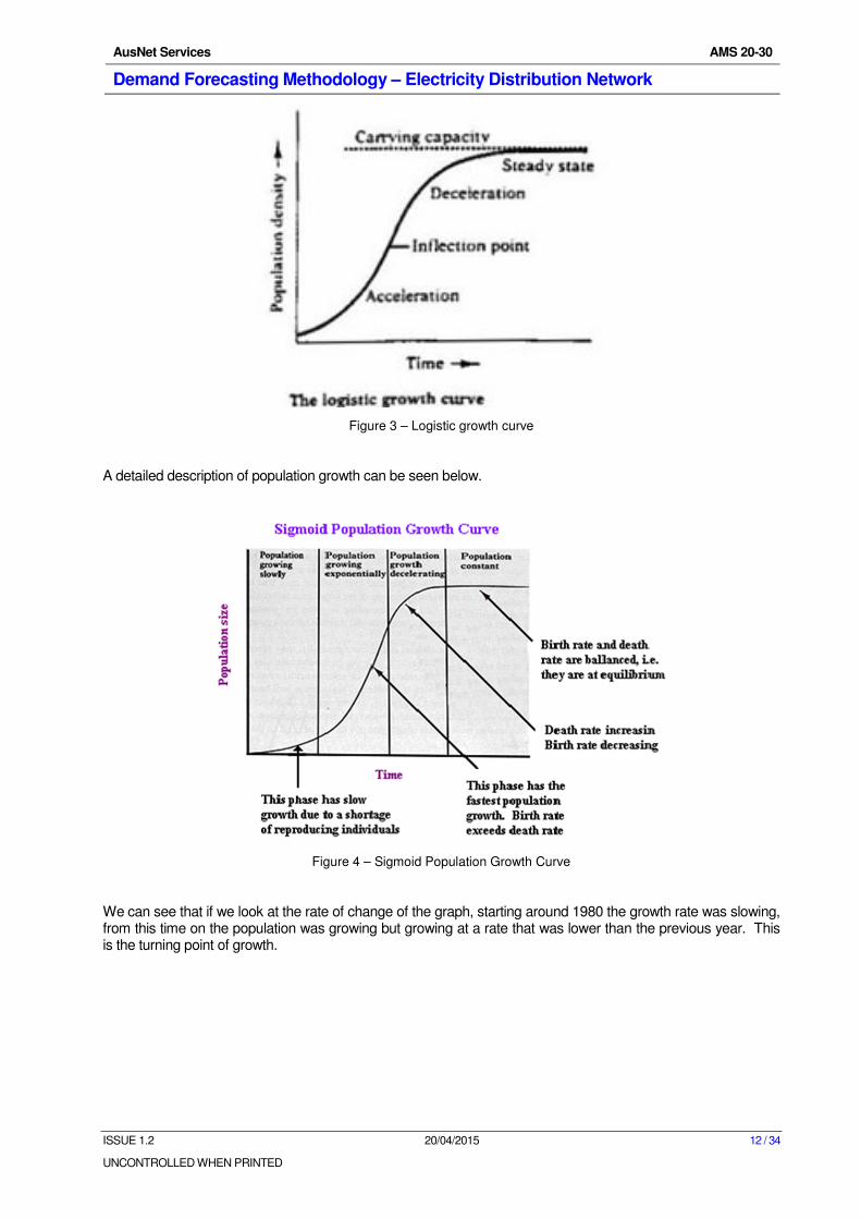
Figure 3 – Logistic growth curve
A detailed description of population growth can be seen below.
Figure 4 – Sigmoid Population Growth Curve
We can see that if we look at the rate of change of the graph, starting around 1980 the growth rate was slowing, from this time on the population was growing but growing at a rate that was lower than the previous year. This is the turning point of growth.
AusNet Services AMS 20-30
Demand Forecasting Methodology – Electricity Distribution Network
ISSUE 1.2 20/04/2015 13 / 34
UNCONTROLLED WHEN PRINTED
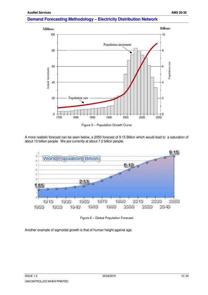
Figure 5 – Population Growth Curve
A more realistic forecast can be seen below, a 2050 forecast of 9.15 Billion which would lead to a saturation of about 10 billion people. We are currently at about 7.2 billion people.
Figure 6 – Global Population Forecast
Another example of sigmoidal growth is that of human height against age.
AusNet Services AMS 20-30
Demand Forecasting Methodology – Electricity Distribution Network
ISSUE 1.2 20/04/2015 14 / 34
UNCONTROLLED WHEN PRINTED
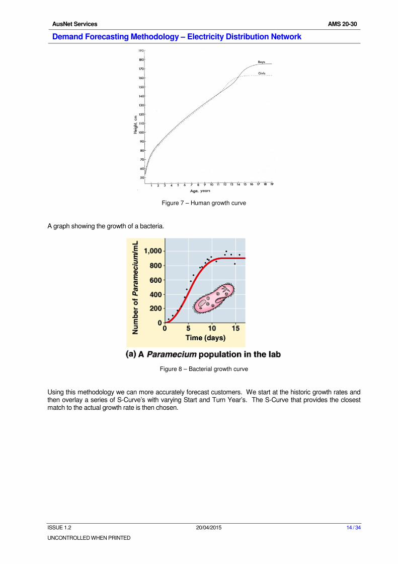
Figure 7 – Human growth curve
A graph showing the growth of a bacteria.
Figure 8 – Bacterial growth curve
Using this methodology we can more accurately forecast customers. We start at the historic growth rates and then overlay a series of S-Curve’s with varying Start and Turn Year’s. The S-Curve that provides the closest match to the actual growth rate is then chosen.
AusNet Services AMS 20-30
Demand Forecasting Methodology – Electricity Distribution Network
ISSUE 1.2 20/04/2015 15 / 34
UNCONTROLLED WHEN PRINTED
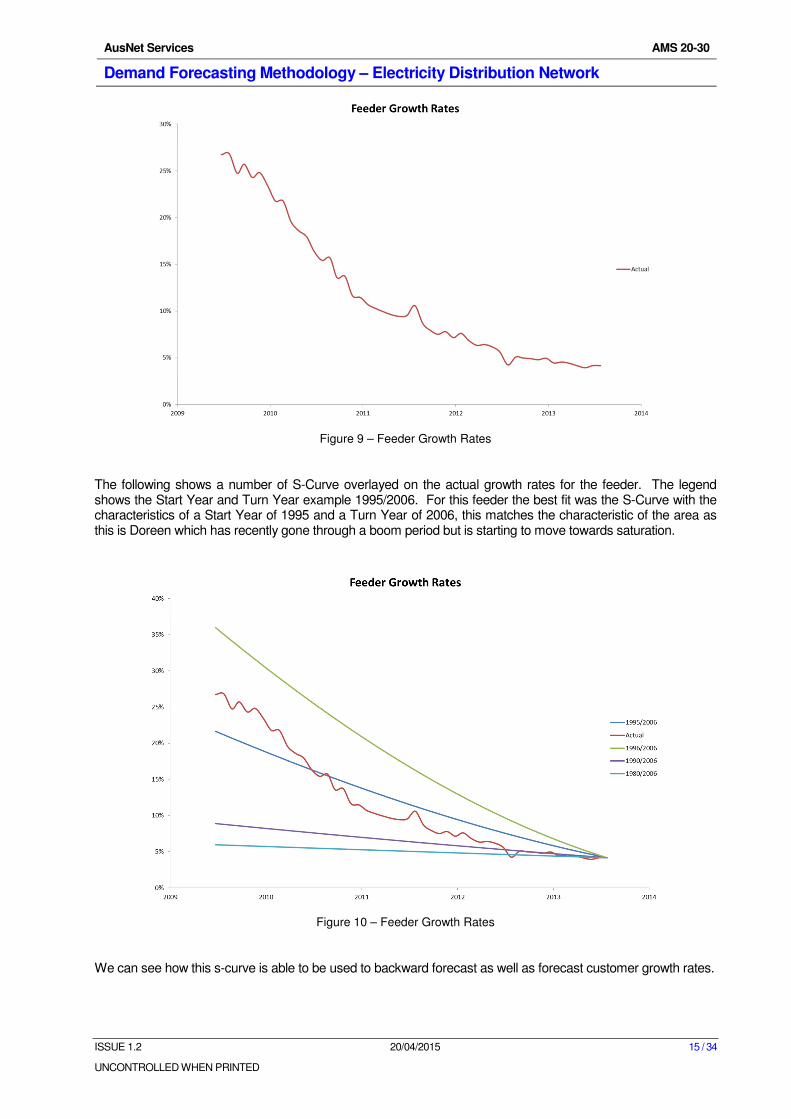
Figure 9 – Feeder Growth Rates
The following shows a number of S-Curve overlayed on the actual growth rates for the feeder. The legend shows the Start Year and Turn Year example 1995/2006. For this feeder the best fit was the S-Curve with the characteristics of a Start Year of 1995 and a Turn Year of 2006, this matches the characteristic of the area as this is Doreen which has recently gone through a boom period but is starting to move towards saturation.
Figure 10 – Feeder Growth Rates
We can see how this s-curve is able to be used to backward forecast as well as forecast customer growth rates.
AusNet Services AMS 20-30
Demand Forecasting Methodology – Electricity Distribution Network
ISSUE 1.2 20/04/2015 16 / 34
UNCONTROLLED WHEN PRINTED
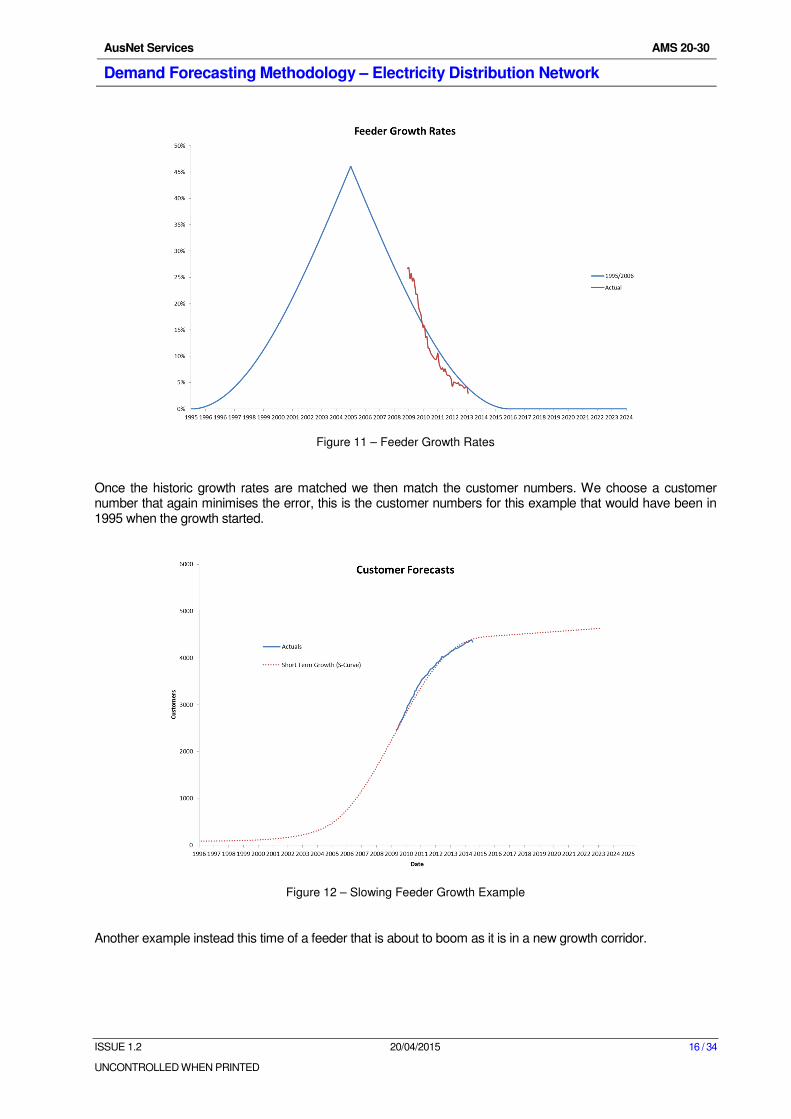
Figure 11 – Feeder Growth Rates
Once the historic growth rates are matched we then match the customer numbers. We choose a customer number that again minimises the error, this is the customer numbers for this example that would have been in 1995 when the growth started.
Figure 12 – Slowing Feeder Growth Example
Another example instead this time of a feeder that is about to boom as it is in a new growth corridor.
AusNet Services AMS 20-30
Demand Forecasting Methodology – Electricity Distribution Network
ISSUE 1.2 20/04/2015 17 / 34
UNCONTROLLED WHEN PRINTED
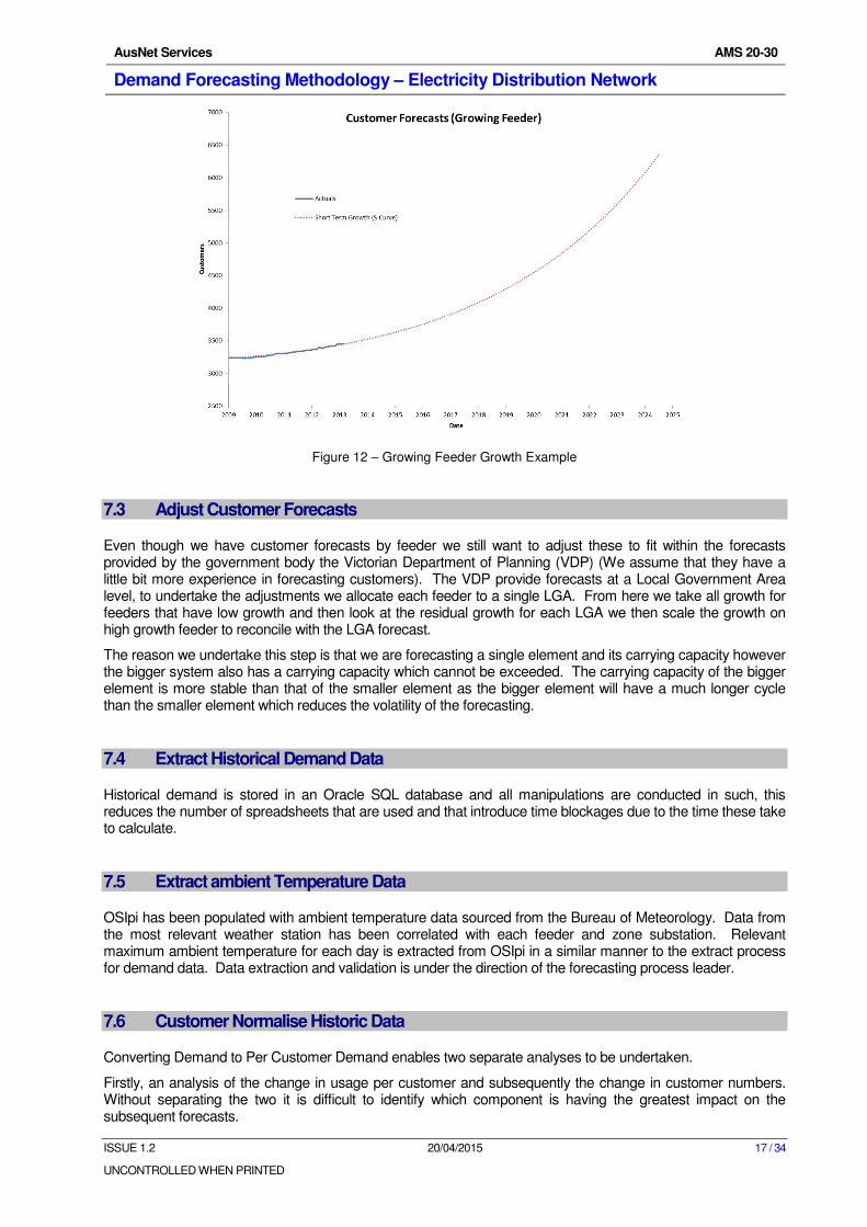
Figure 12 – Growing Feeder Growth Example
7.3 Adjust Customer Forecasts
Even though we have customer forecasts by feeder we still want to adjust these to fit within the forecasts provided by the government body the Victorian Department of Planning (VDP) (We assume that they have a little bit more experience in forecasting customers). The VDP provide forecasts at a Local Government Area level, to undertake the adjustments we allocate each feeder to a single LGA. From here we take all growth for feeders that have low growth and then look at the residual growth for each LGA we then scale the growth on high growth feeder to reconcile with the LGA forecast.
The reason we undertake this step is that we are forecasting a single element and its carrying capacity however the bigger system also has a carrying capacity which cannot be exceeded. The carrying capacity of the bigger element is more stable than that of the smaller element as the bigger element will have a much longer cycle than the smaller element which reduces the volatility of the forecasting.
7.4 Extract Historical Demand Data
Historical demand is stored in an Oracle SQL database and all manipulations are conducted in such, this reduces the number of spreadsheets that are used and that introduce time blockages due to the time these take to calculate.
7.5 Extract ambient Temperature Data
OSIpi has been populated with ambient temperature data sourced from the Bureau of Meteorology. Data from the most relevant weather station has been correlated with each feeder and zone substation. Relevant maximum ambient temperature for each day is extracted from OSIpi in a similar manner to the extract process for demand data. Data extraction and validation is under the direction of the forecasting process leader.
7.6 Customer Normalise Historic Data
Converting Demand to Per Customer Demand enables two separate analyses to be undertaken.
Firstly, an analysis of the change in usage per customer and subsequently the change in customer numbers. Without separating the two it is difficult to identify which component is having the greatest impact on the subsequent forecasts.
AusNet Services AMS 20-30
Demand Forecasting Methodology – Electricity Distribution Network
ISSUE 1.2 20/04/2015 18 / 34
UNCONTROLLED WHEN PRINTED
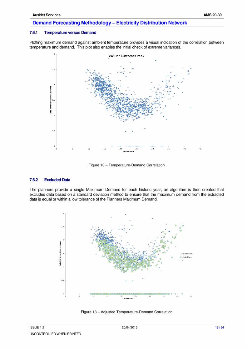
7.6.1 Temperature versus Demand
Plotting maximum demand against ambient temperature provides a visual indication of the correlation between temperature and demand. This plot also enables the initial check of extreme variances.
Figure 13 – Temperature-Demand Correlation
7.6.2 Excluded Data
The planners provide a single Maximum Demand for each historic year; an algorithm is then created that excludes data based on a standard deviation method to ensure that the maximum demand from the extracted data is equal or within a low tolerance of the Planners Maximum Demand.
Figure 13 – Adjusted Temperature-Demand Correlation
AusNet Services AMS 20-30
Demand Forecasting Methodology – Electricity Distribution Network
ISSUE 1.2 20/04/2015 19 / 34
UNCONTROLLED WHEN PRINTED
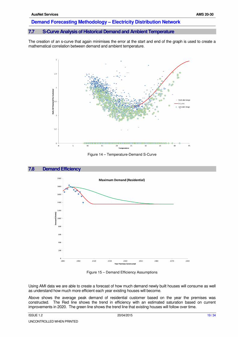
7.7 S-Curve Analysis of Historical Demand and Ambient Temperature
The creation of an s-curve that again minimises the error at the start and end of the graph is used to create a mathematical correlation between demand and ambient temperature.
Figure 14 – Temperature-Demand S-Curve
7.8 Demand Efficiency
Figure 15 – Demand Efficiency Assumptions
Using AMI data we are able to create a forecast of how much demand newly built houses will consume as well as understand how much more efficient each year existing houses will become.
Above shows the average peak demand of residential customer based on the year the premises was constructed. The Red line shows the trend in efficiency with an estimated saturation based on current improvements in 2020. The green line shows the trend line that existing houses will follow over time.
AusNet Services AMS 20-30
Demand Forecasting Methodology – Electricity Distribution Network
ISSUE 1.2 20/04/2015 20 / 34
UNCONTROLLED WHEN PRINTED
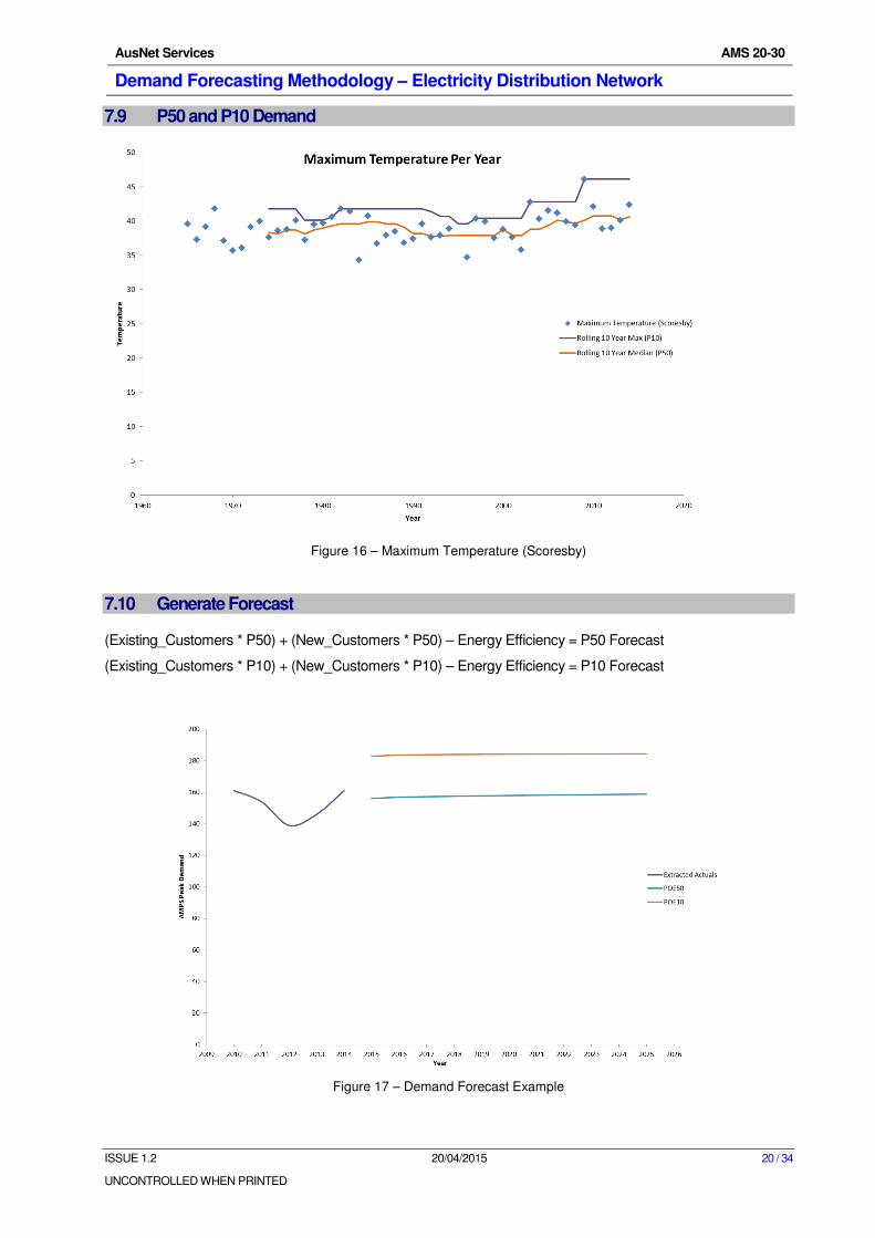
7.9 P50 and P10 Demand
Figure 16 – Maximum Temperature (Scoresby)
7.10 Generate Forecast
(Existing_Customers * P50) + (New_Customers * P50) – Energy Efficiency = P50 Forecast
(Existing_Customers * P10) + (New_Customers * P10) – Energy Efficiency = P10 Forecast
Figure 17 – Demand Forecast Example
AusNet Services AMS 20-30
Demand Forecasting Methodology – Electricity Distribution Network
ISSUE 1.2 20/04/2015 21 / 34
UNCONTROLLED WHEN PRINTED
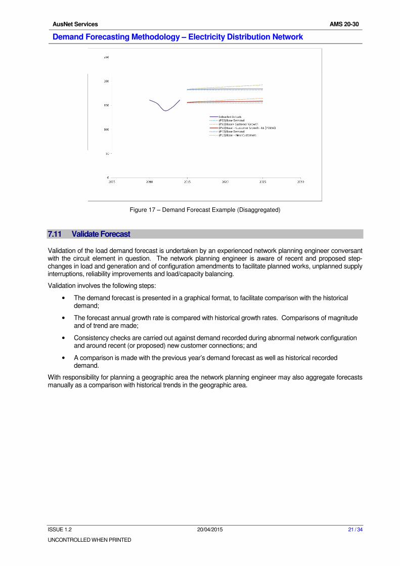
Figure 17 – Demand Forecast Example (Disaggregated)
7.11 Validate Forecast
Validation of the load demand forecast is undertaken by an experienced network planning engineer conversant with the circuit element in question. The network planning engineer is aware of recent and proposed step-changes in load and generation and of configuration amendments to facilitate planned works, unplanned supply interruptions, reliability improvements and load/capacity balancing.
Validation involves the following steps:
• The demand forecast is presented in a graphical format, to facilitate comparison with the historical demand;
• The forecast annual growth rate is compared with historical growth rates. Comparisons of magnitude and of trend are made;
• Consistency checks are carried out against demand recorded during abnormal network configuration and around recent (or proposed) new customer connections; and
• A comparison is made with the previous year’s demand forecast as well as historical recorded demand.
With responsibility for planning a geographic area the network planning engineer may also aggregate forecasts manually as a comparison with historical trends in the geographic area.

AusNet Services AMS 20-30
Demand Forecasting Methodology – Electricity Distribution Network
ISSUE 1.2 20/04/2015 22 / 34
UNCONTROLLED WHEN PRINTED
8 Forecast Outputs
8.1 Draft Forecasts
During the forecasting process draft forecasts are stored in a working folder located at:
• Nsd on cbdshare\\Regulatory & Network Services\Network Strategy & Planning\Forecasting
Network planners can view, review and provide input to draft forecasts in the working folder.
Access to this folder is restricted to members of Regulation and Network Strategy.
8.2 Endorsed Forecasts
Once forecasts are finalised they are placed in a historic forecast folder together with earlier endorsed forecasts also located at:
• Nsd on cbdshare\\Regulatory & Network Services\Network Strategy & Planning\Forecasting
In this location only the forecasting process leader and the lead planner are able to edit the endorsed forecasts. Network planners can view endorsed forecasts in the historic forecast folder.
Access to this folder is restricted to members of Regulation and Network Strategy.
8.3 Archiving
The forecasting process leader is responsible for archiving endorsed forecasts and historic forecasts.
AusNet Services AMS 20-30
Demand Forecasting Methodology – Electricity Distribution Network
ISSUE 1.2 20/04/2015 23 / 34
UNCONTROLLED WHEN PRINTED
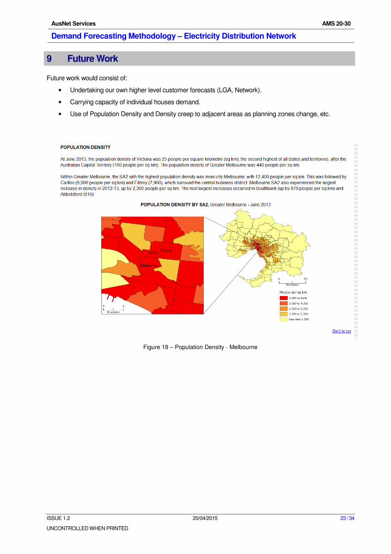
9 Future Work
Future work would consist of:
• Undertaking our own higher level customer forecasts (LGA, Network).
• Carrying capacity of individual houses demand.
• Use of Population Density and Density creep to adjacent areas as planning zones change, etc.
Figure 18 – Population Density - Melbourne

AusNet Services AMS 20-30
Demand Forecasting Methodology – Electricity Distribution Network
ISSUE 1.2 20/04/2015 24 / 34
UNCONTROLLED WHEN PRINTED
10 Notes
This demand forecasting process was first used in 2011.
To manage the transition from the prior multi-technique forecasting processes, which relied heavily on the local knowledge of geographically based network planning engineers, significant emphasis has been placed on each data and forecast validation stage.
10.1 Unit of Measurement
The unit of measurement (kW, kWh, MW, MVA, MVAR, Amps) has a number of implications on the type of forecast produced.
10.1.1 Feeders
For feeder forecasts both maximum single-phase amps and MVA are analysed. Amps are used to ascertain the highest risk the feeder will bear. While MVA feeder loadings are used for diversification calculations.
10.1.2 Zone Substation
For zone substation forecasts the unit of measurement is MVA, based on the MW and MVAR loading of the transformers. This provides a superior reflection of the loadings experienced by the transformers.
10.1.3 Terminal Station
Terminal Station forecasts are based on MW and MVAR.

AusNet Services AMS 20-30
Demand Forecasting Methodology – Electricity Distribution Network
ISSUE 1.2 20/04/2015 25 / 34
UNCONTROLLED WHEN PRINTED
11 Appendix
This appendix outlines the principle drivers influencing this electricity demand forecasting process.
11.1 Electricity Distribution Code
The Distribution Code also requires a distributor to use best endeavours to:
• assess and record the nature, location, condition and performance of its assets;
• develop and implement plans for the acquisition, creation, maintenance, operation, refurbishment, repair and disposal of its distribution system assets and plans for the establishment and augmentation of transmission connections;
o to comply with the laws and other performance obligations which apply to the provision of distribution services;
o to minimise the risks associated with the failure or reduced performance of assets; and
o in a way which minimises costs to customers taking into account distribution losses; and
• develop, test or simulate and implement contingency plans to deal with events which have a low probability of occurring, but are realistic and would have a substantial impact on customers.
11.2 Electricity Distribution Price Reset 2011-2015
The Australian Energy Regulator’s draft EDPR decision3 contained the following assessment by ACIL Tasman
of the features necessary to produce best practice maximum demand, energy and customer number forecasts:
• Accuracy and unbiasedness – careful management of data (removal of outliers, data normalisation) and forecasting model construction (choosing a parsimonious model based on sound theoretical grounds that closely fits the sample data).
• Transparency and repeatability – as evidenced by good documentation, including documentation of the use of judgment, which ensures consistency and minimises subjectivity in forecasts.
• Incorporation of key drivers – including economic growth, population growth, growth in the number of households, temperature and weather related data (where appropriate), and growth in the numbers of air conditioning and heating systems.
• Model validation and testing – including assessment of statistical significance of explanatory variables, goodness of fit, in-sample forecasting performance of the model against actual data, diagnostic checking of the old models, out of sample forecast performance.
3 Draft decision Victorian electricity distribution network service providers Distribution determination 2011–2015 June 2010.
AusNet Services AMS 20-30
Demand Forecasting Methodology – Electricity Distribution Network
ISSUE 1.2 20/04/2015 26 / 34
UNCONTROLLED WHEN PRINTED
ACIL Tasman also considered the following elements to be relevant to maximum demand forecasting:
• A model with fewer rather than a larger number of variables.
• Spatial (bottom up) forecasts validated by independent system level (top down) forecasts – best practice forecasting requires these forecasts to be prepared independently of each other. The impact of macroeconomic, demographic and weather trends are better able to be identified and forecast in system level data, whereas spatial forecasts are needed to capture underlying characteristics of areas on the network. Generally, ACIL Tasman considered spatial forecasts should be constrained to system level forecasts.
• Weather normalisation – correcting historical loads for abnormal weather conditions is an important aspect of demand forecasting. Long time-series weather and demand data are required to establish a relationship between the two and conduct weather correction. Weather correction is relevant to both system and spatial level forecasts, and ACIL Tasman considered that system level weather correction processes are more sophisticated and robust.
• Adjusting for temporary transfers – spatial data must be adjusted for historical spot loads arising from peak load sharing and maintenance, before historical trends are determined.
• Adjusting for discrete block loads – large new developments (for example, shopping centres, housing developments) should be incorporated into the forecasts, taking account of the probability that each development might not proceed. Only block loads exceeding a certain size threshold should be included in the forecasts, to avoid potential double counting, as historical demands incorporate block loads.
• Incorporation of maturity profile of service area in spatial time series – recognising the phase of growth of each zone substation, taking account of the typical lifecycle of a zone substation, depending on its age, helps to inform likely future growth rates.
11.3 Historic Analysis
Historic analysis methods have been included to show how previous demand forecasting was undertaken and to show how we have arrived at our current forecasting methodology.
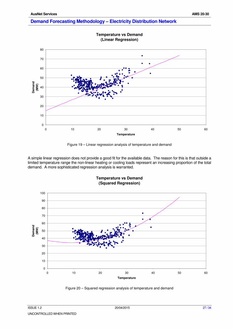
11.3.1 Temperature versus Demand
Analysing and calculating the correlation between demand and temperature is a critical step in forecasting. Research has been conducted into the most appropriate analysis technique for describing the correlation between temperature and demand. In calculating these correlations a suitable technique is to undertake regression analysis. When undertaking regression analysis any number of input variables (Temperature, Temperature Squared, etc) can be compared to a single output (Demand).
Investigations into how many input variables to use and how to cut the output data to provide the most accurate correlation has been undertaken.
AusNet Services AMS 20-30
Demand Forecasting Methodology – Electricity Distribution Network
ISSUE 1.2 20/04/2015 27 / 34
UNCONTROLLED WHEN PRINTED
Figure 19 – Linear regression analysis of temperature and demand
A simple linear regression does not provide a good fit for the available data. The reason for this is that outside a limited temperature range the non-linear heating or cooling loads represent an increasing proportion of the total demand. A more sophisticated regression analysis is warranted.
Figure 20 – Squared regression analysis of temperature and demand
Temperature vs Demand
(Linear Regression)
0
10
20
30
40
50
60
70
80
0 10 20 30 40 50 60
Temperature
Dem
an
d
(MW
)
Temperature vs Demand
(Squared Regression)
0
10
20
30
40
50
60
70
80
90
100
0 10 20 30 40 50 60
Temperature
Dem
an
d
(MW
)
AusNet Services AMS 20-30
Demand Forecasting Methodology – Electricity Distribution Network
ISSUE 1.2 20/04/2015 28 / 34
UNCONTROLLED WHEN PRINTED
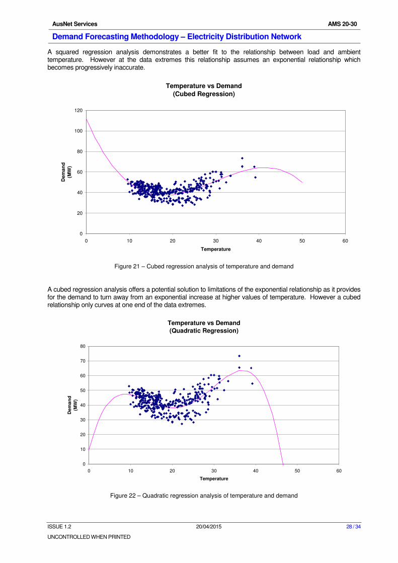
A squared regression analysis demonstrates a better fit to the relationship between load and ambient temperature. However at the data extremes this relationship assumes an exponential relationship which becomes progressively inaccurate.
Figure 21 – Cubed regression analysis of temperature and demand
A cubed regression analysis offers a potential solution to limitations of the exponential relationship as it provides for the demand to turn away from an exponential increase at higher values of temperature. However a cubed relationship only curves at one end of the data extremes.
Figure 22 – Quadratic regression analysis of temperature and demand
Temperature vs Demand
(Cubed Regression)
0
20
40
60
80
100
120
0 10 20 30 40 50 60
Temperature
De
ma
nd
(MW
)
Temperature vs Demand
(Quadratic Regression)
0
10
20
30
40
50
60
70
80
0 10 20 30 40 50 60
Temperature
De
ma
nd
(MW
)
AusNet Services AMS 20-30
Demand Forecasting Methodology – Electricity Distribution Network
ISSUE 1.2 20/04/2015 29 / 34
UNCONTROLLED WHEN PRINTED
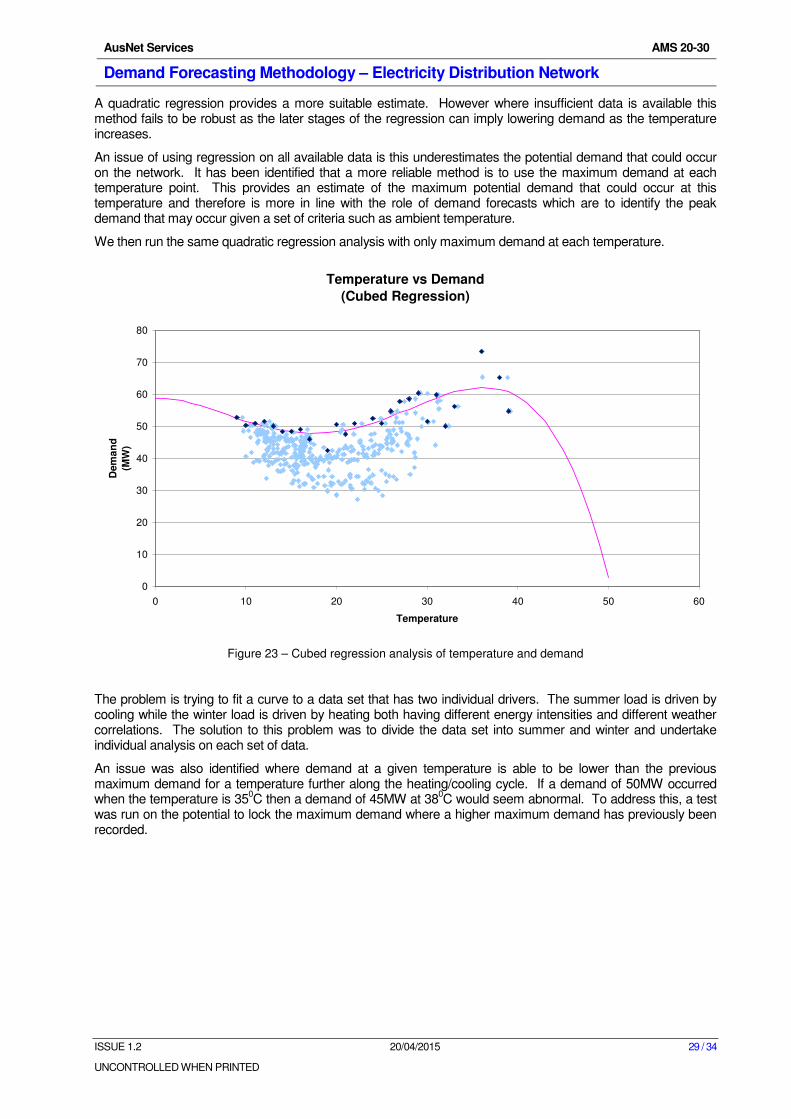
A quadratic regression provides a more suitable estimate. However where insufficient data is available this method fails to be robust as the later stages of the regression can imply lowering demand as the temperature increases.
An issue of using regression on all available data is this underestimates the potential demand that could occur on the network. It has been identified that a more reliable method is to use the maximum demand at each temperature point. This provides an estimate of the maximum potential demand that could occur at this temperature and therefore is more in line with the role of demand forecasts which are to identify the peak demand that may occur given a set of criteria such as ambient temperature.
We then run the same quadratic regression analysis with only maximum demand at each temperature.
Figure 23 – Cubed regression analysis of temperature and demand
The problem is trying to fit a curve to a data set that has two individual drivers. The summer load is driven by cooling while the winter load is driven by heating both having different energy intensities and different weather correlations. The solution to this problem was to divide the data set into summer and winter and undertake individual analysis on each set of data.
An issue was also identified where demand at a given temperature is able to be lower than the previous maximum demand for a temperature further along the heating/cooling cycle. If a demand of 50MW occurred when the temperature is 35
0C then a demand of 45MW at 38
0C would seem abnormal. To address this, a test
was run on the potential to lock the maximum demand where a higher maximum demand has previously been recorded.
Temperature vs Demand
(Cubed Regression)
0
10
20
30
40
50
60
70
80
0 10 20 30 40 50 60
Temperature
Dem
an
d
(MW
)
AusNet Services AMS 20-30
Demand Forecasting Methodology – Electricity Distribution Network
ISSUE 1.2 20/04/2015 30 / 34
UNCONTROLLED WHEN PRINTED
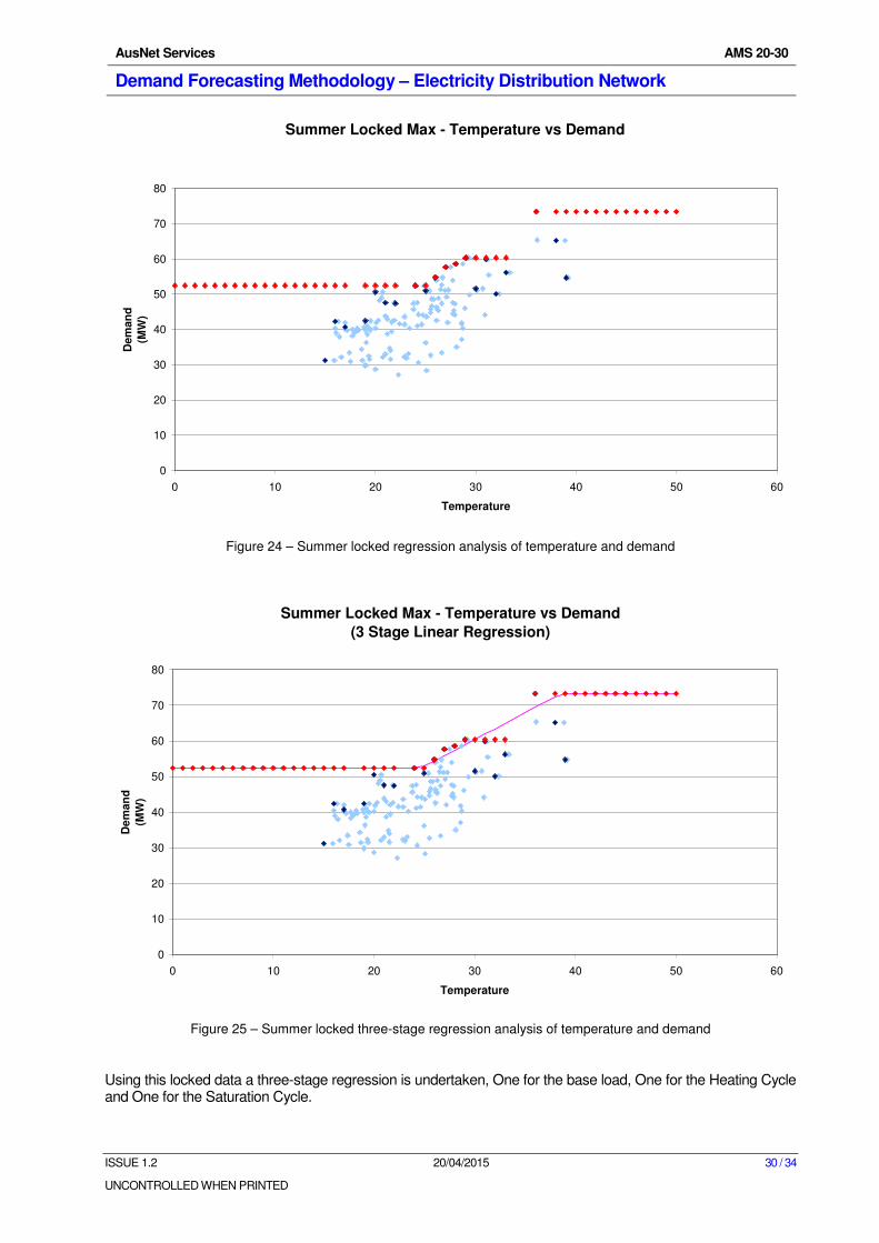
Figure 24 – Summer locked regression analysis of temperature and demand
Figure 25 – Summer locked three-stage regression analysis of temperature and demand
Using this locked data a three-stage regression is undertaken, One for the base load, One for the Heating Cycle and One for the Saturation Cycle.
Summer Locked Max - Temperature vs Demand
0
10
20
30
40
50
60
70
80
0 10 20 30 40 50 60
Temperature
De
man
d
(MW
)
Summer Locked Max - Temperature vs Demand
(3 Stage Linear Regression)
0
10
20
30
40
50
60
70
80
0 10 20 30 40 50 60
Temperature
De
man
d
(MW
)
AusNet Services AMS 20-30
Demand Forecasting Methodology – Electricity Distribution Network
ISSUE 1.2 20/04/2015 31 / 34
UNCONTROLLED WHEN PRINTED
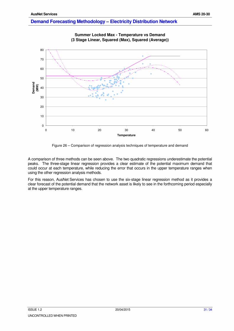
Figure 26 – Comparison of regression analysis techniques of temperature and demand
A comparison of three methods can be seen above. The two quadratic regressions underestimate the potential peaks. The three-stage linear regression provides a clear estimate of the potential maximum demand that could occur at each temperature, while reducing the error that occurs in the upper temperature ranges when using the other regression analysis methods.
For this reason, AusNet Services has chosen to use the six-stage linear regression method as it provides a clear forecast of the potential demand that the network asset is likely to see in the forthcoming period especially at the upper temperature ranges.
Summer Locked Max - Temperature vs Demand
(3 Stage Linear, Squared (Max), Squared (Average))
0
10
20
30
40
50
60
70
80
0 10 20 30 40 50 60
Temperature
Dem
an
d
(MW
)

AusNet Services AMS 20-30
Demand Forecasting Methodology – Electricity Distribution Network
ISSUE 1.2 20/04/2015 32 / 34
UNCONTROLLED WHEN PRINTED
11.4 Summer Preparedness Process Review
In December 2010 an audit was conducted on the AusNet Services Summer preparedness process. The following summarised the findings of that audit.
Summer Preparedness Process Review
Company: AusNet Services
Division: Networks Strategy & Development
Department: Regulation & Network Strategy
Month and Year of Audit: December 2010
Risk Rating: Medium
Issue Reference: 8.2
Title of Audit Issue: Demand forecasting to be consistent and robust
Description of Audit Issue:
Inconsistent forecast models and practice:
Inconsistent forecast practice was observed among regions. Different methods and horizons were used to arrive at the growth rates for ZSS forecasts:
Central: Growth rate was derived straight-line on historical actual demand ignoring the regression model. The Planner would then decide on one of the two rates generated from the past 3 years and 10 years based on knowledge of load profile changes but such assumptions were not documented. For 2010/11 the calculated growth rates were adjusted to reconcile with high level NIEIR system growth rate for EDPR submission purposes.
Eastern: Similar to Central, NIEIR – adjusted growth rates were utilised for all ZSS forecast in the region. These adjusted rates were significantly different from the calculated rates from regression analysis on historical actual demands. While the adjustments may have been valid, the explanation and rationale behind significant variances were not documented.
Northern: Growth rate was derived from an average of 7-year historical actual demand data. The planner rejected regression model as unsuitable, based on his local knowledge.
The adjustments of growth rates at ZSS level determined on historical, internal data to the external NIEIR system growth rate reflected two different methodologies, and effectively broke the consistency in AusNet Services’ ZSS growth forecasts and the underlying assumptions. Although aggregately and globally at network level, AusNet Services’ growth rate had been reconciled to be consistent with NIEIR’s, adjusted rates at times fluctuated significantly from historically calculated rates at the local ZSS level. Concern arose where such adjustments may be inconsistent with the actual ZSS load profiles therefore impacting on demand forecast into future years.
AusNet Services AMS 20-30
Demand Forecasting Methodology – Electricity Distribution Network
ISSUE 1.2 20/04/2015 33 / 34
UNCONTROLLED WHEN PRINTED
Summer Preparedness Process Review
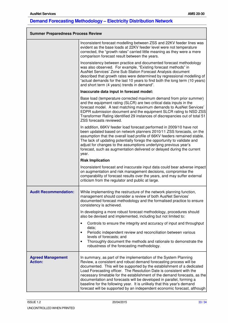
Inconsistent forecast modelling between ZSS and 22KV feeder lines was evident as the base loads at 22KV feeder level were not temperature corrected, the “growth rates” carried little meaning as they were a mere comparison forecast result between the years.
Inconsistency between practice and documented forecast methodology was also observed. For example, “Existing forecast methods” in AusNet Services’ Zone Sub Station Forecast Analysis document described that growth rates were determined by regressional modelling of “actual demands for the last 10 years to find both the long term (10 years) and short term (4 years) trends in demand”.
Inaccurate data input in forecast model:
Base load (temperature corrected maximum demand from prior summer) and the equipment rating (SLCR) are two critical data inputs in the forecast model. A test matching maximum demands to AusNet Services’ EDPR submission document and the equipment SLCR rating to NSD ZSS Transformer Rating identified 29 instances of discrepancies out of total 51 ZSS forecasts reviewed.
In addition, 66KV feeder load forecast performed in 2009/10 have not been updated based on network planners 2010/11 ZSS forecasts, on the assumption that the overall load profile of 66KV feeders remained stable. The lack of updating potentially forego the opportunity to validate and adjust for changes to the assumptions underlying previous year’s forecast, such as augmentation delivered or delayed during the current year.
Risk Implication
Inconsistent forecast and inaccurate input data could bear adverse impact on augmentation and risk management decisions, compromise the comparability of forecast results over the years, and may suffer external criticism from the regulator and public at large.
Audit Recommendation: While implementing the restructure of the network planning function, management should consider a review of both AusNet Services’ documented forecast methodology and the formalised practice to ensure consistency is achieved.
In developing a more robust forecast methodology, procedures should also be devised and implemented, including but not limited to:
• Controls to ensure the integrity and accuracy of input and throughput data;
• Periodic independent review and reconciliation between various levels of forecasts; and
• Thoroughly document the methods and rationale to demonstrate the robustness of the forecasting methodology.
Agreed Management Action:
In summary, as part of the implementation of the System Planning Review, a consistent and robust demand forecasting process will be documented. This will be supported by the establishment of a dedicated Load Forecasting officer. The Resolution Date is consistent with the necessary timetable for the establishment of the demand forecasts, as the documentation and forecasts will be developed in parallel, forming a baseline for the following year. It is unlikely that this year's demand forecast will be supported by an independent economic forecast, although

AusNet Services AMS 20-30
Demand Forecasting Methodology – Electricity Distribution Network
ISSUE 1.2 20/04/2015 34 / 34
UNCONTROLLED WHEN PRINTED
Summer Preparedness Process Review
that is the intention for future years.
Action:
• Load demand forecasting methodologies will be well documented and consistently followed for the different regions.
Outcomes:
• Consistent methodologies for all three regions.
• Introduce version and spreadsheet controls.
• Improve process and access control to safeguard data integrity. (Original is currently kept by planner).
Action:
• Input data (maximum demand and plant ratings) will be reviewed to ensure accuracy.
Outcomes:
• This relates mainly to plant data, with corrections to be made for the 2011 forecast.
Action:
• Growth rate and network configuration assumptions will be validated.
Outcomes:
• Abnormal system configurations are being assessed but will ensure that processes are improved and that this is consistent for all regions.
Action:
• Single point of accountability will improve the process and the demand forecasts.
Outcomes:
• Subject to Planning Review, implementation of the new structure and appointment of a person responsible for load demand forecasting.