Embed Size (px)
Citation preview
1
Augmenting a Conceptual Model with Geo-spatio-temporal Annotations1
Vijay Khatri*, Sudha Ram** and Richard T. Snodgrass**
*Indiana University, Bloomington IN 47405; **University of Arizona, Tucson AZ 85721
Abstract: While many real-world applications need to organize data based on space (e.g., geology, geo-marketing, environmental modeling) and/or time (e.g., accounting, inventory management, personnel management), existing conventional conceptual models do not provide a straightforward mechanism to explicitly capture the associated spatial and temporal semantics. As a result, it is left to database designers to discover, design and implement—on an ad-hoc basis—the temporal and spatial concepts that they need. We propose an annotation-based approach that allows a database designer to focus first on non-temporal and non-geospatial aspects (i.e., “what”) of the application, and subsequently augment the conceptual schema with geo-spatio-temporal annotations (i.e., “when” and “where”). Via annotations, we enable a supplementary level of abstraction that succinctly encapsulates the geo-spatio-temporal data semantics and naturally extends the semantics of a conventional conceptual model. An overarching assumption in conceptual modeling has always been that expressiveness and formality need to be balanced with simplicity. We posit that our formally defined annotation-based approach is not only expressive but also straightforward to understand and implement. Index Terms: Data Semantics, Database Design, Semantic Model, Geospatial Databases and Temporal Databases 1 Introduction Many real-world geo-referenced (e.g., land information systems, environmental modeling,
transportation planning, geo-marketing, geology, archaeology) and time-varying (e.g.,
accounting, portfolio management, personnel management, inventory management) applications
need to organize data based on space and/or time. Underlying these applications are temporal
and/or geospatial data, collectively referred to as geo-spatio-temporal data. Conceptual database
design is widely recognized as an important step in the development of database applications [1,
3, 7] such as those listed above. During conceptual database design, a conceptual model provides
a notation and formalism that can be used to construct a high-level description of the real
world—referred to as the conceptual schema—independent of implementation details. The data
1 This work was supported in part by NASA grant 314401, NSF grants EIA-0080123 and IIS-0100436, and by a grant from the Boeing Corporation. The authors thank the associate editor and the anonymous reviewers for their insightful comments.

2
semantics provides a mapping from the conceptual schema to aspects in the real world. However,
conventional conceptual models [1, 3, 7] do not provide a straightforward mechanism to
explicitly capture the semantics related to space and time. As a result, it is left to the database
designers to discover, design and implement—on an ad-hoc basis—the temporal and spatial
concepts that they need. In this paper, we present a methodical approach that augments a
conventional conceptual model using geo-spatio-temporal annotations.
Many prior studies [10, 23] attribute project failures to lack of identifying real needs during
conceptual design. One of the problems with developing geo-spatio-temporal applications is that
there is “a gulf between the richness of knowledge structures in the application domains and the
relative simplicity of the data model in which the structures can be expressed” [33], which in
turn impacts the ability to elicit the application requirements. Considering that geographic data
are finding their way into traditional applications (e.g., insurance, retail, distribution), there is a
need for an overall geo-spatio-temporal conceptual database design methodology that can be
integrated into conventional conceptual design. Thus, it would be helpful to develop an approach
that is compatible with an existing general-purpose methodology, e.g., [1, 3, 7].
Our annotation-based approach divides geo-spatio-temporal conceptual design into two
steps: (i) elicit the current reality of an application using a conventional conceptual model
without considering the geospatial and temporal aspects (“what”) and only then (ii) annotate the
schema with the geo-spatio-temporal semantics of the application (“when” and “where”). Rather
than creating new constructs in a conceptual model, we use annotations to elicit the geo-spatio-
temporal aspects of the application. Our annotation-based approach is generic and can be applied
to any conventional conceptual model [1, 3, 7] to transform that model into a geo-spatio-
temporal conceptual model. In this paper, we apply our annotation-based approach to the
3
Unifying Semantic Model (USM) [22]—an extended version of the Entity-Relationship (ER)
Model [3]—to propose the geo-Spatio-Temporal Unifying Semantic Model (ST USM).
We mention here the assumptions in this paper to delineate the scope of our work. (i) Based
on perception, space may be differentiated as large-scale and small-scale [17]. As with Mark and
Frank [19], we construe large-scale space as equivalent to geographic space. In the following, we
use the term space interchangeably to mean large-scale space or geographic space. (ii) According
to Peuquet [21], absolute space is objective since it provides an immutable structure that is
purely geometric. On the other hand, relative space is an ordering relation between objects that
determines their relative position. We concentrate on absolute representations, which are
typically employed in databases. (iii) A database schema can evolve with time. Schema
versioning [24] is an important area of research; however, we do not focus on schema
versioning. In summary, this paper focuses on establishing a foundation for capturing the geo-
spatio-temporal data semantics during conceptual design and does not delve into peripheral
research areas.
The rest of the paper is organized as follows. In Section 2, we outline requirements related to
geo-spatio-temporal conceptual modeling. According to Wand et al. [31], “the power of a
modeling language lies in the semantics of its constructs” and “ontology can be used to define
concepts that should be represented by the modeling language.” The basis for annotations is the
time and space ontology summarized in Section 3. We describe our annotation-based geo-spatio-
temporal conceptual design methodology, which first focuses on “what” is important for an
application in the real world and then associates “what” with “when” and/or “where.” In Section
4, we summarize a conventional conceptual model, USM, which provides various abstractions to
capture “what” is important for an application. In Section 5, we apply our annotation-based

4
approach to USM to realize ST USM, which captures the semantics related to “when” and/or
“where.” We round out the paper with evaluation and contributions. In this paper, we provide the
essence of our approach; complete details are available in a comprehensive report [15].
2 Desiderata A precursor to designing and developing a geo-spatio-temporal conceptual model is identifying
the conceptual modeling requirements that need to be met. Based on a hydrogeologic study at the
US Geological Survey (USGS), we provide an example of an application that needs to capture
the geo-spatio-temporal data semantics. We then outline the evaluation criteria for a conceptual
model that can capture the data semantics for geo-spatio-temporal applications like that at the
USGS.
2.1 Hydrogeologic Application We are working with a group of researchers who are developing a ground-water flow model [5]
for the Death Valley region in the state of Nevada. Beneath the earth's surface, there is a zone
where all interstices are filled with water referred to as ground water. The objective of the
ground-water flow model is to characterize regional 3D ground-water flow paths so that policy-
makers can make decisions related to radionuclide contaminant transport and the impact of
ground water pumping on national parks and local communities in the region. However, the
quality of the model output and the predictions based on these models are dependent on the data
that forms an input to these models.
A large part of the input data for this model is geospatial and/or temporal in nature. For
example, two key objects of interest in the application are spring-water sites and borehole sites.
Both these objects need to be spatially referenced to the earth. A spring-water site is represented
as a point whose location on the surface of the earth is given by the geographic x- and y-co-
ordinates, with a geospatial granularity of degree. Spring-water sites are points where spring

5
discharge is measured. Similar to springs, boreholes are access points to the ground water
system. Information of their construction and condition are important for monitoring ground
water supply and remediation. A borehole site refers to a part of the borehole whose 3D location
is given by the x- and y-co-ordinates on the earth’s surface with a geospatial granularity of
degree, along with the depth below land surface with a geospatial granularity of foot; there can be
different borehole sites at different depths at the same surface location. Physically, a borehole is
composed of hole-intervals with different diameters. A borehole can also be thought to be
composed of a sequence of casings and openings. A casing is a section of a borehole with
concrete, steel or plastic installed on the borehole. An opening is a section of a borehole that is
open to allow water flow. Additionally, a borehole site may have associated access tubes that
provide access to a section of the borehole. Casings, openings, hole interval and access tubes
define the characteristics of a borehole, and the water-level measurements taken at the borehole
site are influenced by these aspects.
A primary input data for the ground-water flow model includes discharge (in cubic feet per
second) at a spring-water site and water depth (in feet below land surface) at a borehole site, both
of which are collected by a source agency. Discharge and water depth need to be associated with
the time of measurement (in minute). The researchers evaluate the collected water level and
discharge measurements to decide which of them will be included as input for the ground-water
flow model; the measurements used as an input to the model are referred to as io-water-level
(that is, input-output water level) and io-discharge (that is, input-output discharge), respectively.
There are various hydraulic tests conducted at the borehole site and the results of these tests need
to be coupled with the time (in minute) when the test was conducted. Additionally, a borehole site

6
may have a pumplift that removes water from the borehole site; the existence of a pumplift can
affect other data collected at the borehole site.
Capturing the data semantics related to, e.g., spring-water site, borehole site, borehole,
casing, water level, source agency, requires a proposed spatio-temporal conceptual model to: (i)
allow the data analyst to model non-geospatial, non-temporal, geospatial and temporal aspects of
the application in a straightforward manner; (ii) provide a framework for expressing the structure
of spatio-temporal data that is easily understood and communicated to the users; (iii) support a
mechanism for a methodical translation into implementation-dependent logical models; and (iv)
include a mechanism to represent various spatial and temporal granularities (e.g., minute, second,
degree) in a conceptual schema.
Having summarized some of the requirements for a typical geospatial application, we next
describe evaluation criteria for a geo-spatio-temporal conceptual model designed to capture the
data semantics illustrated above.
2.2 Evaluation Criteria Batini et al. [1] posit that conceptual models should possess the following qualities:
expressiveness, simplicity, minimality and formality. Additionally, to augment extant
conventional conceptual models [1, 3, 7] with geo-spatio-temporal concepts, we need to take into
account upward compatibility and snapshot reducibility [2].
Expressiveness refers to the availability of a large variety of concepts for a more
comprehensive representation of the real world. Wand et al. [31] posit that “conceptual modeling
can be anchored in the models of human knowledge” and that ontology be employed as the basis
for a proposed formalism. One of the conflicting goals related to expressiveness is simplicity,
which requires that the schema developed using a conceptual model be understandable to both

7
users and data analysts. Prior research [20] contends that one of the deficiencies of the existing
conceptual models that can represent geographic phenomena is their inability to “represent
information in way that is more natural to humans.” While minimality ensures that no concept
can be expressed through composition of other concepts, formality specifies that the model must
present a unique, precise and well-defined interpretation. Similarly, Wand et al. [32] posit that
effective use of conceptual modeling constructs requires that their meaning be defined
“rigorously.”
Upward compatibility [2] refers to the ability to render a conventional conceptual schema
geo-spatio-temporal without impacting or negating that legacy schema, thus protecting
investment in the existing schemas. It also implies that both the legacy schemas and the geo-
spatio-temporal schemas can co-exist. Upward compatibility requires that the syntax and
semantics of the traditional conceptual model [1, 3, 7] remain unaltered. Snapshot reducibility
[2] implies a “natural” generalization of the syntax and semantics of extant conventional
conceptual models [1, 3, 7] for incorporating the geo-spatio-temporal extension. Snapshot
reducibility ensures that the semantics of geo-spatio-temporal model are understandable in terms
of the semantics of the conventional conceptual model. Here, the overall objective is to help
ensure minimum additional investment in a data analyst training.
Juhn and Naumann [13] posit that conceptual representations “drive discovery” and should
be precisely and rigorously defined; on the other hand, discovery needs to be “validated,” and the
schemas should be clear and comprehensible. In essence, the challenge of adding the space and
time dimension is balancing simplicity and understandability with preciseness and completeness.
3 Ontology-based Geo-spatio-temporal Semantics Geographic applications require data referenced by geographic co-ordinates, with time
sometimes referred to as the fourth dimension. We summarize key temporal, geospatial and

8
time-varying geospatial terminology in this section. Next, we describe the annotation syntax and
illustrate how ontology is the basis for annotations.
3.1 Temporal Ontology A time domain is denoted by the pair (T, ≤), where T is a nonempty set of time instants and “≤”
is a total order on T. We assume that the time domain is discrete (as the measurements modeled
are captured at a time known to a discrete value). For example, (Z, ≤) represents a discrete time
domain where instants are denoted by integers, implying that every instant has a unique
successor. An instant is a point on the time line. The time between two instants is referred to as a
time period. An unanchored contiguous portion of the time line is called a time interval, e.g., one
day (or Gregorian day). Unlike time periods, a time interval is a directed duration of time with
“no specific starting or ending instants” [11]. A non-decomposable time interval of fixed minimal
duration is referred to as a chronon. A finite union of non-overlapping time periods is referred to
as a temporal element [8].
A temporal granularity—an integral part of the temporal data—is defined as a mapping TG
from index i to subsets of the time domain [6]. Although the index of a temporal granularity is
constrained to be contiguous, the granules are not constrained to be contiguous on the time
domain. Thus, a temporal granularity defines a countable set of non-decomposable granules
TG(i). Additionally, a special granule called the origin, TG(0), is non-empty. Some examples of
temporal granularities are Gregorian-day (with each such granule composed of a sequence of 24
contiguous Gregorian-hour granules, or 86,400 contiguous Gregorian-second granules), business-day
and business-week (with each such granule composed of five Gregorian-day granules). While
Gregorian-day is a temporal granularity with contiguous granules of day, business-day contains
some non-contiguous granules (e.g., Friday is followed directly by Monday). Each non-empty

9
granule may have a textual representation referred to as a label (e.g., “2001-10-5 EST”), which
can be mapped to an index integer with label mapping. A designated point of time is referred to
as an anchor with respect to the time domain. The union of granules is called an image of a
temporal granularity.
Facts can interact with time in two orthogonal ways resulting in transaction time and valid
time [28]. Valid time denotes when the fact is true in the real world and implies the storage of
histories related to facts. Existence time, which applies to an object, is the valid time when the
object exists. On the other hand, transaction time links an object to the time it is current in the
database and implies the storage of versions of a database object. While the temporal granularity
can be specified for existence time and valid time, that for transaction time is system-defined.
Time-varying data may be modeled as an event or a state. An event occurs at a point of time, i.e.,
an event has no duration. A state has duration, e.g., a storm occurred from 5:07 PM to 5:46 PM.
3.2 Geospatial Ontology Any data that can be associated to a location on the earth is referred to as geographic data. A
space domain may be represented as a set (e.g., R3, R2, N3, N2) with elements referred to as
points. For geographic applications, horizontal space is segregated from vertical space;
correspondingly, we define horizontal and vertical geospatial granularities [16]. Intuitively, the
horizontal space domain corresponds to the earth’s surface while the vertical space domain
corresponds to the depth/height below/above the sea level. We define a horizontal geospatial
granularity as a mapping from integers to any partition of the horizontal space; the partition may
arise from pixellation of space and may be a regular square or any other shape like triangular
irregular network (TIN) or even irregular shapes (e.g., county). Examples of horizontal geospatial
granularities are dms-deg, dms-min and county.

10
A geospatial object is associated with position and geometry. The position in space is based
on the co-ordinates in a reference system, e.g., latitude and longitude. Geometry represents the
shape of an object: a point, a line and a region. A point is “a zero-dimensional geospatial object
with co-ordinates,” a line is “a sequence of ordered points, where the beginning of the line may
have a special start node and the end a special end node” and a region consists of “one outer and
zero or more inner rings” [30]. The difference between a line and a region is that the line itself is
the carrier of information, while the area is of primary importance for a region.
3.3 Time-Varying Geospatial Ontology In geography, space is indivisibly coupled with time. Three types of interaction between an
object and space-time are possible [29]: (i) moving objects, i.e., objects whose position changes
continuously but the shape does not (e.g., a car moving on a road network); (ii) objects whose
geospatial characteristics and position change with time discretely, i.e., changing shape (e.g., a
change in the shape of land parcels for a cadastral application); and, (iii) integration of the above
two behaviors, i.e., continuous moving and changing phenomena (e.g., modeling a storm).
Having summarized the temporal, geospatial and time-varying geospatial semantics that need
to be captured in a geo-spatio-temporal conceptual model, we describe how ontology manifests
into annotations.
3.4 Geo-spatio-temporal Annotations Annotations provide a mechanism to specify the context (“when” and “where”) associated with
“what” is important in the real world. As shown in Figure 1, the overall structure of an
annotation phrase is:
⟨temporal annotation⟩ // ⟨geospatial annotation⟩ // ⟨time-varying geospatial annotation⟩.

11
The temporal annotations, geospatial annotations, and time-varying geospatial annotations are
each separated by a double forward slash (//).
The temporal annotation first specifies existence time (or valid time) followed by transaction
time. The temporal annotation for existence time and transaction time is segregated by a forward
slash (/). Any of these aspects can be specified as not being relevant to the associated conceptual
construct by using “-”. Valid time or existence time can be modeled as an event (E) or a state (S)
and has an associated temporal granularity. For example, “S(min)/T//” associated with DISCHARGE
denotes that DISCHARGE exists in a bitemporal space and that the temporal granularity of the
states (S) is minute (min). Additionally, we also need to capture transaction time (T) associated
with DISCHARGE. In this example, the granularity associated with transaction time is not
specified, as it is system-defined.
The geospatial annotation includes geometry and position in x-, y- and z-dimension, and each
dimension is segregated by a forward slash (/). For example, “// P(deg) / P(deg) / -” for
SPRING_SITE describes a geometry of points (P) in the x-y plane. The associated horizontal
geospatial granularity is degree.
The interaction between an object and space-time can result in a change in the shape and/or a
change in the position of an object. A time-varying geospatial annotation can be specified only if
geospatial and temporal annotation have already been specified. For example, a moving car
tracked by satellite may be represented by an annotation phrase “E(sec) / - // P(deg) / P(deg) / - //
Pos@xy” that denotes a time-varying position and a time-invariant shape. The geometry is a point
(P) in the x-y plane with geospatial granularity of degree. The position changes in the x-y plane
(Pos@xy) over time and each geometry is valid for time granules (E) measured in second. Our

12
annotation also includes a formalism to model indeterminacy; details related to modeling
indeterminacy can be found elsewhere [16].
Figure 1: Annotation Syntax in BNF
Having outlined geo-spatio-temporal annotations, we next apply our annotation-based
approach to a conventional conceptual model, USM, to propose a geo-spatio-temporal
conceptual model called ST USM. However, our annotation-based approach is not specific to
⟨annotation⟩ ::= є | ⟨temporal annotation⟩ // ⟨spatial annotation⟩ | ⟨temporal annotation⟩ // ⟨spatial annotation⟩ // ⟨time-varying spatial annotation⟩
⟨temporal annotation⟩ ::= є | ⟨valid time⟩ / ⟨transaction time⟩ ⟨valid time⟩ ::= ⟨state⟩ (⟨gt⟩) | ⟨indeterminate state⟩ (⟨gt⟩) | ⟨event⟩ (⟨gt⟩) | ⟨indeterminate event⟩(⟨gt⟩) | - ⟨transaction time⟩ ::= T | - ⟨state⟩ ::= S | State ⟨indeterminate state⟩ ::= ⟨state⟩~ | ⟨state⟩+- ⟨event⟩ ::= E | Event ⟨indeterminate event⟩ ::= ⟨event⟩~ | ⟨event⟩+- ⟨spatial annotation⟩ ::= є | ⟨horizontal geometry⟩ / ⟨vertical geometry⟩ ⟨horizontal geometry⟩ ::= ⟨geometry⟩ (⟨gxy⟩) / ⟨geometry⟩ (⟨gxy⟩) ⟨vertical geometry⟩ ::= ⟨geometry⟩ (⟨gz⟩) | - ⟨geometry⟩ ::= ⟨point⟩ | ⟨indeterminate point⟩ | ⟨line⟩ | ⟨indeterminate line⟩ | ⟨region⟩
| ⟨indeterminate region⟩ | ⟨user defined⟩ | - ⟨point⟩ ::= P | Point ⟨indeterminate point⟩ ::= ⟨point⟩~ | ⟨point⟩+- ⟨line⟩ ::= L | Line ⟨indeterminate line⟩ ::= ⟨line⟩~ | ⟨line⟩+- ⟨region⟩ ::= R | Region ⟨indeterminate region⟩ ::= ⟨region⟩~ | ⟨region⟩+- ⟨time-varying spatial annotation⟩ ::= є | ⟨position varying⟩ | ⟨shape varying⟩ | ⟨position varying⟩ / ⟨shape varying⟩ ⟨position varying⟩ ::= ⟨position⟩@⟨varying in dimension⟩ ⟨shape varying⟩ ::= ⟨shape⟩@⟨varying in dimension⟩ ⟨position⟩ ::= Pos | Position ⟨shape⟩ ::= Sh | Shape ⟨varying in dimension⟩ ::= x | y | z | xy | yz | xz | xyz ⟨gt⟩ ::= ⟨day⟩ | ⟨hour⟩ | ⟨minute⟩ | ⟨second⟩ | ⟨user defined⟩ ⟨day⟩ ::= day ⟨hour⟩ ::= hr | hour ⟨minute⟩ ::= min | minute ⟨second⟩ ::= sec | second ⟨gxy⟩ ::= ⟨dms-degree⟩ | ⟨dms-minute⟩ | ⟨user defined⟩ ⟨gz⟩ ::= ⟨mile⟩ | ⟨foot⟩ | ⟨user defined⟩ ⟨mile⟩ ::= mile ⟨dms-degree⟩ ::= dms-deg | dms-degree ⟨dms-minute⟩ ::= dms-min | dms-minute ⟨foot⟩ ::= ft | foot

13
USM and can be applied to any conventional conceptual model [3, 7]. In the next two sections,
we exemplify our geo-spatio-temporal conceptual modeling methodology via USM and ST
USM.
4 USM: Representing “what” The abstractions supported by typical conventional conceptual models [1, 3, 7, 22, 27] include
classification, association, aggregation and generalization/specialization. The underlying
principle of these abstractions is selective emphasis of detail. We summarize below the data
semantics that can be elicited using conventional conceptual modeling, specifically USM. Figure
2 illustrates a USM schema that represents “what” is important for the hydrogeologic application
described in Section 2.
All real world objects are referred to by the term entity. Characteristics or properties of
entities are called attributes (Ai, where i = 1, …, n). Each attribute has an attribute domain
(dom(Ai)), which is the set of values that an entity can take for the attribute. An entity class (or
class) may be defined as E = ∪i (Ai, dom(Ai)). The set of instantiations of an entity class is
referred to as an entity set. In other words, an entity e of an entity class E may be designated as
e(E) and a set of entities of an entity class is represented as S(E) where
e(E) ∈ S(E). For example in Figure 2, PUMPLIFT is an entity class which has attributes like serial
number (serial_no), manufacturer (mfg), type and installation date (installation_date).
An interaction relationship refers members of one entity class to members of one or more
entity classes. Formally, let R be an interaction relationship and E1, E2, …, En be classes that
participate in the relationship. A relationship may be considered to be a subset of the Cartesian
product S(E1) × S(E2) ×…× S(En), where a relationship instance ri consists of exactly one entity
from each participating entity set. For example in Figure 2, is_in is an interaction relationship
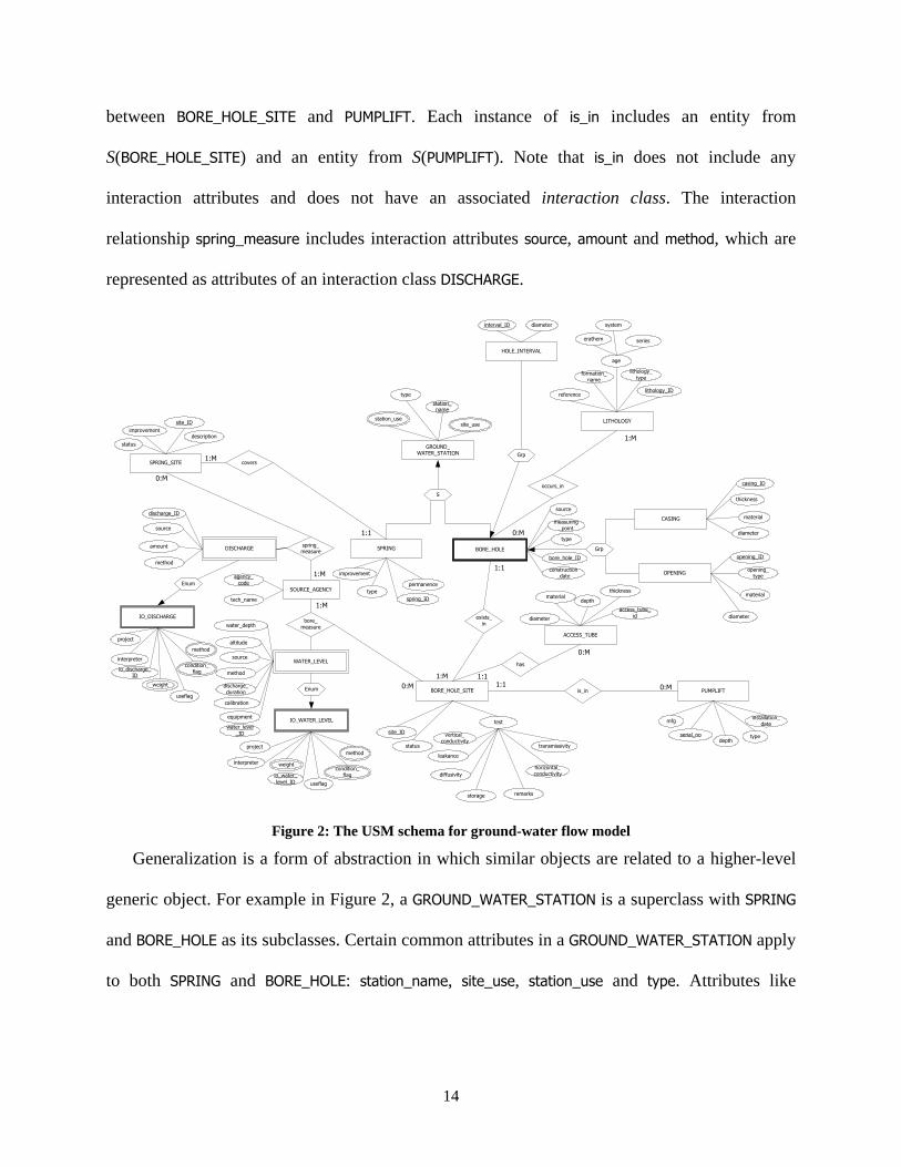
14
between BORE_HOLE_SITE and PUMPLIFT. Each instance of is_in includes an entity from
S(BORE_HOLE_SITE) and an entity from S(PUMPLIFT). Note that is_in does not include any
interaction attributes and does not have an associated interaction class. The interaction
relationship spring_measure includes interaction attributes source, amount and method, which are
represented as attributes of an interaction class DISCHARGE.
GROUND_WATER_STATION
BORE_HOLESPRING
HOLE_INTERVAL
CASING
OPENING
PUMPLIFTis_in
station_name
Grp
occurs_in
LITHOLOGY
SOURCE_AGENCY
spring_measure Grp
WATER_LEVEL
bore_measure
S
serial_no
DISCHARGE
site_use
0:M1:1
1:M
1:M
0:M
type
opening_type
material
1:M
0:M
interval_ID
test
transmissivity
horizontal_conductivity
vertical_conductivity
leakance
diffusivity
storage
agency_code
tech_name
amount
source
method
water_depth
source
BORE_HOLE_SITE
SPRING_SITE
site_ID
improvement
diameter
site_ID
1:1
exists_in
1:1
0:M
covers
1:1
1:M
station_use
method
installation_date
typedepth
mfg
construction_date
source
diameter
diameter
material
thickness
formation_name
permanence
remarks
discharge_duration
lithology_type
referencelithology_ID
status
opening_ID
casing_ID
statusdescription
IO_WATER_LEVEL
Enum
project
useflag
condition_flag
method
interpreter
IO_DISCHARGE
project
useflag
condition_flag
method
interpreter
Enum
calibration
altitude
equipment
type
type
age
erathem
system
series
ACCESS_TUBE
has
diameter
materialthickness
access_tube_id
0:M
1:M
improvement
measuring_point
depth
weight
weight
discharge_ID
io_discharge_ID
water_level_ID
io_water_level_ID
bore_hole_ID
spring_ID
Figure 2: The USM schema for ground-water flow model
Generalization is a form of abstraction in which similar objects are related to a higher-level
generic object. For example in Figure 2, a GROUND_WATER_STATION is a superclass with SPRING
and BORE_HOLE as its subclasses. Certain common attributes in a GROUND_WATER_STATION apply
to both SPRING and BORE_HOLE: station_name, site_use, station_use and type. Attributes like

15
permanence and improvement are specific to SPRING. On the other hand, construction_date and
measuring_point are attributes that are associated with BORE_HOLE.
A composite relationship defines a new class called a composite class that has another entity
set (or subsets of an entity set) as its members. For example, IO_DISCHARGE is a composite class
with DISCHARGE as its component class. Note that the component class DISCHARGE is both a
subclass and a subtype of the composite class IO_DISCHARGE.
The grouping establishes a “part-of” or “property-of” relationship. For example, BORE_HOLE
is a grouping class with CASING and OPENING as its component classes. Unlike IO_DISCHARGE (a
composite class), BORE_HOLE (a grouping class) is not of the same type as CASING or OPENING
(component classes).
In this section, we described briefly the semantics associated with a conventional conceptual
model, USM. We next explicate the semantics of annotation-based ST USM using USM and
constraints in first-order logic.
5 ST USM: Representing “when” and “where” Using an example of a temporal entity class, we show the detailed semantics of an annotated
abstraction. Details related to other abstractions like attribute, interaction relationship, subclass,
composite class and grouping class are similar to those of a temporal entity class and described
elsewhere [15]. The goal is to provide here the essence of our approach.
5.1 Entity Class An application may require capturing the lifespan or transaction time of an entity, the shape and
position of an entity in space, or a change in the shape and/or position of an entity over its
lifespan, resulting in a temporal entity class, a geo-spatial entity class, or a time-varying geo-
spatial entity class, respectively.

16
5.1.1 Temporal Entity Class In a temporal entity class, the membership of an entity in the entity set is time-varying. We
assume that a temporal entity class itself (as contrasted with entities of that class) exists during
the entire modeled time. Thus, the existence time represents the lifespan of an entity and defines
the time when facts associated with an entity can be true in the miniworld. Similarly, we can
capture the transaction time associated with an entity, which may be important for applications
requiring traceability.
A temporal entity class, e.g., PUMPLIFT, with existence time is associated with an existence
time predicate ϕPUMPLIFT,et that defines the lifespan of a pumplift in terms of an existence time
granularity TGPUMPLIFT,et (e.g., day). ϕPUMPLIFT,et: S(PUMPLIFT) × Z → B. This predicate takes a
particular pumplift entity and a particular granule (denoted by an integer, here a specific day) of
the granularity and evaluates to a Boolean that is true if that entity exists in the modeled reality at
that granule (day). There are two constraints on the existence time predicate:
(i) ∀ e ∈ S(PUMPLIFT), ∀ i, ϕPUMPLIFT,et(e, i) ⇒ (TGPUMPLIFT,et(i) ⊆ Image(TGPUMPLIFT,et))
(ii) ∀ e ∈ S(PUMPLIFT), ∃ i ∈ Z, ϕPUMPLIFT,et (e, i)
The first constraint states that a pumplift can exist only within the defined image of the
granularity. Second, every entity exists at some granule (e.g., “2001-7-01”) within the image of
the granularity. Intuitively, if a pumplift with an associated lifespan does not exist during any
granule within the image, it is meaningless to store it in the database. We define an existence
temporal projection operator (πet) as a function that takes a temporal entity and returns the
associated temporal element.
Similarly, a temporal entity class PUMPLIFT with transaction time is associated with a
transaction time predicate ϕPUMPLIFT,tt that defines the transaction time of a pumplift in terms of a

17
transaction time granularity TGtt (e.g., second). The transaction time granularity is defined only
for all points less than now. If a transaction timestamp includes Until Changed (UC, a special
transaction time marker), it denotes that the associated fact is current in the database. Unlike the
existence time granularity, which can be specified by users, the transaction time granularity is
system-defined. ϕPUMPLIFT,tt: S(PUMPLIFT) × {Z ∪ UC} → B. The constraints on the transaction
time predicate are similar to those on the existence time predicate. In the same way, a bitemporal
entity class PUMPLIFT is associated with ϕPUMPLIFT,et and ϕPUMPLIFT,tt defined in terms of an existence
time granularity TGPUMPLIFT,et and a transaction time granularity TGtt, respectively.
Having defined temporal entity class abstractly, we next describe its semantics using an
example of PUMPLIFT. When an entity class is defined as temporal, it implies that the application
would have queries like “What is the average monthly power consumption by all pumplifts over
their installed existence?” and “What are the pumplifts that were installed before 1995 and are
operational now?” Figure 3 illustrates the representation of existence time expressed as state (S)
with day as the temporal granularity name. The data analyst simply annotates PUMPLIFT based on
the users’ requirements with “S(day)/-//” (as shown in the top part of the figure) and does not
need to contend with the complexity of the underlying semantics (shown in the bottom part of
the figure) or of the associated temporal constraints. Figure 3 presents the semantics of a
temporal entity class in ST USM via a mapping using the concepts of a conventional conceptual
model, which we refer to as a translated USM schema. Note how the spatio-temporal semantics
encapsulated via annotations in the ST USM schema are “unpacked” in the translated USM
schema. This rendition from an ST USM schema to a (translated) USM schema is snapshot
equivalent, that is, the two schemas (ST USM and translated USM) represent the same
information content over snapshots taken at all times.

18
In order to express the semantics of a temporal entity class, we need to specify a
TEMPORAL_GRANULARITY in which the evolution of a temporal object is embedded. The
relationship PUMPLIFT_has_ET associates an entity with a corresponding TEMPORAL_GRANULARITY.
Each TEMPORAL_GRANULARITY is uniquely identified by a granularity_name, shown by an
underlined attribute. An extent is the smallest time interval that includes the image of the
granularity and is expressed by two indexes, minimum and maximum. Each anchor_gran is a
recursive relationship (i.e., a relationship where an entity from the same entity class can play
different roles) such that each participating granularity optionally has an anchor (0:1) and each
granularity is an anchor for potentially many other granularities (0:M).
PUMPLIFT
S (day) / - //
TEMPORAL_GRANULARITY
anchor
PUMPLIFT_has_ET
1:10:M
USM
ST USM
granularity_name
anchor_gran
0:M
begin end
state_periods
PUMPLIFT
extent
groups_into
maximum
minimum
0:M
0:M
0:1
ishas
coarser-than
finer-than
Figure 3: Temporal Entity Class in ST USM and its semantics in USM
The anchor of a granularity TG is the first index of a strictly finer granularity that corresponds to
the origin of this granularity, i.e., TG(0). All granularities except the bottom granularity have an
associated anchor. A finer-than and a coarser-than relationship between granularities are denoted
by a recursive relationship groups_into, where one granularity plays the role of finer-than and the
other the role of coarser-than. The relationships anchor_gran together with groups_into help create

19
a granularity graph [6], which can aid a designer in choosing the level of detail associated with
facts. Details related to granularities and indeterminacy vis-à-vis ST USM are presented
elsewhere [16].
A temporal entity with existence time may have a set of event_instants or state_periods
associated with it, depending on whether a temporal entity is represented as an event or a state. A
time period of PUMPLIFT is represented with indexes begin and end of state_periods. A double-
lined ellipse in USM denotes a multi-valued attribute. For example, state_periods is represented
as a multi-valued attribute and represents a set of state periods (i.e., a temporal element)
associated with an entity.
We now describe the constraints on temporal entities of PUMPLIFT. These inherent constraints
in the ST USM schema are rendered as explicit constraints in the translated USM schema.
Constraints 5.1.1 and 5.1.2 are based on our definition of a temporal entity, i.e., a temporal entity
has an associated temporal granularity and has an associated temporal element. Constraints
5.1.3−5.1.5 are based on the definition of a temporal element. In these definitions, we assume a
closed-open representation, i.e., the begin index is contained in the period while the index
corresponding to the end is not. For example, an instant for a temporal element may be
represented by [17, 18). In this example, begin index (i.e., 17) is inclusive in the instant while end
index (i.e., 18) is not.
Constraint 5.1.1: The existence time for all the entities of PUMPLIFT have the same associated granularity; in this case, day.
∀ e ∈ S(PUMPLIFT), e.PUMPLIFT_has_ET.TEMPORAL_GRANULARITY (granularity_name) = day Constraint 5.1.2: Every entity of PUMPLIFT has an associated temporal element with well-formed periods.
∀ e ∈ S(PUMPLIFT), ∃p ∈ e.state_periods, p.begin < p.end Constraint 5.1.3: State periods of an entity of PUMPLIFT are well-formed.
∀ e ∈ S(PUMPLIFT), ∀p ∈ e.state_periods, p.begin < p.end Constraint 5.1.4: Temporal elements are well-formed. A temporal element is defined as a union of non-overlapping time intervals.
∀ e ∈ S(PUMPLIFT), ∀ p1, p2 ∈ e.state_periods, p1.begin < p2.begin ⇒ p1.end ≤ p2.begin

20
Constraint 5.1.5: The extent of a temporal granularity defines the upper and lower bounds for any temporal element. In other words, a temporal element cannot include an index that is larger than the corresponding extent.maximum or smaller than the corresponding extent.minimum.
∀ e ∈ S(PUMPLIFT), ∀ p ∈ e.state_periods, e.PUMPLIFT_has_ET.TEMPORAL_GRANULARITY (extent.minimum) ≤ p.begin < p.end ≤ e.PUMPLIFT_has_ET.TEMPORAL_GRANULARITY (extent.maximum)
Constraints 5.2.1−5.2.3 are based on the definition of a temporal granularity. These
constraints will be generated once for the entire schema.
Constraint 5.2.1: Each TEMPORAL_GRANULARITY has a lower and an upper bound referred to as minimum and maximum; these bounds are well-formed.
∀ e ∈ S(TEMPORAL_GRANULARITY), e(extent.minimum) < e(extent.maximum) Constraint 5.2.2: All the granularities, except one, have an anchor. In other words, the bottom granularity is allowed not to have an anchor.
∀ e1 ∈ S(TEMPORAL_GRANULARITY), ¬ has(e1.anchor_gran) ⇒ ¬ (∃ e2 ∈ S(TEMPORAL_GRANULARITY) ∧ e1 ≠ e2 ∧ ¬ has(e2.anchor_gran))
Constraint 5.2.3: For a temporal granularity, if an anchor does not exist then that is the bottom granularity that does not have any granularity finer than it; in other words, it cannot take the role of coarser-than in the relationship groups-into.
∀ e ∈ S(TEMPORAL_GRANULARITY), ¬ has(e.anchor_gran) ⇒ ¬ coarser-than(e.groups_into) As exemplified by an example of PUMPLIFT, the temporal annotation associated with an entity
class renders it sequenced, i.e., the entity exists for each point in time (specified by granularity
indexes) within the specified lifespan. Note how the annotation phrase (e.g., “S(day)/-//”)
associated with an entity class encapsulates the semantics that are explicated in Figure 3 and
constraints 5.1.1−5.1.5 and 5.2.1−5.2.3. As may be evident, an easily-expressed annotation
phrase may represent a quite complex semantics via this mapping.
5.1.2 Geospatial Entity Class A geospatial entity class refers to geo-referenced entities with an associated shape and position,
which is used to locate them in a two- or three-dimensional space. In this subsection, we first
define a geospatial entity in terms of a geospatial granularity and then describe the associated
semantics of a geospatial entity class in ST USM, using examples of SPRING_SITE and
BORE_HOLE_SITE.
A geospatial entity in a horizontal space domain, e.g., SPRING_SITE, is associated with a
horizontal geometry predicate ψSPRING_SITE,xy that defines the location of a spring site in terms of
horizontal geospatial granularity. ψSPRING_SITE,xy: S(SPRING_SITE) × Z → B.

21
Spatial partitions—formed in a 2- or 3-dimensional space—are represented by integers.
Constraints on horizontal geometry predicate are similar to those on the existence time predicate.
We can define a horizontal geospatial projection operator (πxy) that takes a geospatial entity and
returns its geometry (point, line or region). In the case of SPRING_SITE, πxy is constrained to be a
point on the horizontal surface.
A geospatial entity in 3-dimensional space, e.g., BORE_HOLE_SITE, is associated with
ψBORE_HOLE_SITE,xy and ψBORE_HOLE_SITE,z that defines the location of an entity in terms of horizontal and
vertical geospatial granularities, i.e., SGBORE_HOLE_SITE,xy and SGBORE_HOLE_SITE,z, respectively. For an
entity in 3-dimensional space, we define a vertical geospatial projection operator, πz. In the
example above, πxy is constrained to be a point and πz is constrained to be a line.
The semantics of a geospatial entity class can be defined like those for a temporal entity class
described in the previous section [15].
5.1.3 Time-Varying Geospatial Entity Class A time-varying geospatial entity class models two types of changes: (i) non-geospatial change
refers to an entity with a fixed associated position/geometry and a lifespan; and (ii) geospatial
change denotes an entity whose geometry varies over its lifespan. While the former models a
geospatial entity with an associated existence time (and/or transaction time), the latter captures a
change in shape and/or position over time (existence time and/or transaction time) [29]. For the
second case, only the position of an entity may change continuously while its shape does not
(e.g., a transportation application), or the shape may change discretely (e.g., a cadastral
application), or both position and shape may change continuously (e.g., modeling a hurricane).
For the first case, a time-varying geospatial entity class is associated with an existence
predicate (i.e., ϕE,et), a (horizontal) geometry predicate (i.e., ψE,xy), and the geospatial projection

22
is not time-varying. Intuitively, this implies that the application needs to capture when and where
entities exist. However, queries that involve evolving geometries over time like “During the year
2001, did the surface area of Lake Mesquite decrease by more than 10% of its area measured on
2000-08-25” are not required of the application. The annotation for this case is simply a
combination of the geospatial and temporal annotation already described in the previous two
subsections.
For the second case above, the application needs to capture various shapes and/or positions
of the entities over time. Our annotation syntax includes a formalism to specify whether position
(Pos or Position) and/or shape (Sh or Shape) is time-varying. Additionally, the user can also
specify the dimension (e.g., xy and xyz) over which the position and/or shape changes over time.
However, to include a time-varying geospatial annotation, the temporal and geospatial
annotation should already have been specified. The time-varying geospatial annotation is
specified after the second double forward slash (//). For example, “S(min)/-// R(dms-sec)/ R(dms-
sec)/-//Sh@xy” implies that the shape of entities is a region (R) in an x-y plane with a horizontal
geospatial granularity of dms-second. The shape of the entity changes over time in the x-y plane
(Sh@xy) and each shape is valid for a set of time granules (S ≡ state) measured in minute. If the
geometry changes from a region to a point (or even line), the geometry is still generically
represented as region (R) only, as a point (or a line) is a degenerate region.
The semantics of a time-varying geospatial entity class can be defined like those for a
temporal entity class [15].
5.2 Attribute Entities have properties referred to as attributes that represent facts that need to be captured for a
database application. An entity class can have two kinds of attributes, descriptive attributes and

23
geospatial attributes. If the user wants to elicit the evolution of facts over time, the attribute is
referred to as a temporal attribute. On the other hand, when the user wants to capture the
evolution of geospatial facts over time, the attribute is referred to as a time-varying geospatial
attribute.
5.2.1 Temporal Attribute Temporal attributes represent properties of an entity that are associated with valid time and/or
transaction time. The temporal annotation for an attribute is the same as that for a temporal entity
class described in the previous section. Annotating an attribute renders it sequenced, implying
that the property is true for each point in time within the associated temporal element.
As shown in Table 1, a non-temporal or temporal attribute can be associated with a temporal
or non-temporal entity class. A temporal entity class implies that objects are pertinent for a
database application even when they are not current in the modeled reality. A non-temporal
entity class implies that only the currently legitimate objects are important for the database
application. If a non-temporal entity is no longer currently legitimate, one does not need to store
the evolution of facts associated with such an entity (cell 2 in Table 1). For example, a non-
temporal entity class SOURCE_AGENCY with a temporal attribute tech_name would imply that
histories of only currently relevant source agencies are pertinent for the application. A non-
temporal attribute of a temporal entity (cell 3 in Table 1) indicates that: (i) the attribute does not
vary with time; (ii) the user is only interested in the last recorded value of the attribute and not in
its history; or (iii) the time associated with the attribute is unknown. A temporal attribute for a
temporal entity class (cell 4 in Table 1) necessitates that the valid time of the attribute is equal to
the lifespan of the entity, which is a direct implication from the semantics of a conventional
conceptual model where attributes are specified for an existing entity. Cell 1 in Table 1

24
represents a non-temporal entity class with non-temporal attribute in a conventional conceptual
model with implicit snapshot semantics.
Non-temporal Attribute Temporal Attribute Non-temporal Entity Class
Only the current properties of the currently relevant entities (1)
Maintain attribute value histories of the currently relevant entities (2)
Temporal Entity Class/ Time varying geospatial Entity Class
Only the current properties over the lifespan of entities (3)
Maintain attribute value histories over the lifespan of entities (4)
Table 1: The semantics of temporal/non-temporal attribute/entity combinations
Note how snapshot reducibility naturally extends (i.e., cell 2, 3 and 4) the conventional semantics
shown in grey (i.e., cell 1).
A single-valued temporal attribute is one where each entity has a maximum of one value for
any time granule; however, it can have multiple values over the lifetime of the entity. A temporal
attribute A of an entity class E with valid time is associated with an attribute valid time function
ϕE,A,vt that defines the attribute values, dom(A), at different time granularity indexes. ϕE,A,vt: S(E)
× Z → 2dom(A) . The constraints on the attribute valid time function are described below:
(i) ∀ e ∈ S(E), ϕE,A,vt (e, i) ∈ dom(A) ⇒ (TGE,A,vt(i) ⊆ Image(TGE,A,vt))
(ii) ∀ e ∈ S(E), ∀ i, ϕE,et (e, i) ⇒ ϕE,A,vt (e, i) ∈ dom(A)
The first constraint states that the history of an attribute can be defined within the image of the
granularity of the attribute. The second constraint—which applies when the associated attribute
of a temporal entity is also temporal (cell 4 of Table 1)—states that the history of an attribute is
defined within the lifespan of the associated entity. If no value is defined for a granularity index
where an entity exists, the corresponding value of the temporal (optional) attribute for that index
is assumed to be unknown; this is a direct implication from the semantics of a conventional
conceptual model where optional attributes [22] imply properties with unknown values. Similar
to mandatory attributes that are required to have a non-null value, temporal mandatory attributes

25
are required to have non-null values at each point in time (i.e., a sequenced constraint). This is
natural generalization of the definition of a mandatory attribute. While a single-valued temporal
attribute, ϕE,A,vt(e,i) is constrained to be a singleton (i.e., a set with only one element), no such
restriction exists for a multi-valued temporal attribute.
Similar to a temporal attribute with valid time, a temporal attribute with transaction time is
associated with an attribute transaction function ϕE,A,tt and a bitemporal attribute is associated
with ϕE,A,tt and ϕE,A,vt.
We now describe the constraints on a temporal attribute. The constraints related to a temporal
element are similar to 5.1.3−5.1.5. The granularity-based constraints 5.2.1−5.2.3 hold for a
temporal attribute also. The constraint 5.3.1 is a sequenced consequent of a (non-temporal)
USM, where an attribute (e.g., attr) draws values from a domain (e.g., dom(attr) ∪ NULL); a
temporal attribute draws values from the domain at each point in time during the lifespan of the
entity.
Constraint 5.3.1: If both the entity class and its attribute are temporal, the union of the temporal elements of an (temporal) attribute (ap) must be equal to the lifespan of the associated entity (ep).
∀ e ∈ S(⟨ENTITY_CLASS⟩), ∀ ep ∈ e.state_periods, ∀ k ∈ [ep.begin, ep.end), ∃ a ∈ e.⟨ENTITY_CLASS⟩_⟨t-attrib⟩_REL.⟨ENTITY_CLASS⟩_⟨t-attrib⟩, ∃ ap ∈ a.state_periods,
ap.begin ≤ k < ap.end
Identifiers (also called keys) are one or more attributes used to identify members of an entity
set. Annotating a key attribute renders it sequenced. In other words, a temporal key—a
sequenced constraint—is a uniqueness constraint at each point in time.
Constraint 5.3.2: If ⟨t-attrib⟩ is a key attribute, there will be an additional uniqueness constraint on this attribute. At each point of time within the temporal element, the number of entities with the same value of the key attribute is 1.
∀ e1, e2 ∈ S(⟨ENTITY_CLASS⟩), ∃a1 ∈ e1.⟨ENTITY_CLASS⟩_⟨t-attrib⟩_REL.⟨ENTITY_CLASS⟩_⟨t-attrib⟩, ∃a2 ∈ e2.⟨ENTITY_CLASS⟩_⟨t-attrib⟩_REL.⟨ENTITY_CLASS⟩_⟨t-attrib⟩, ∃p1 ∈ a1.state_periods,
∃p2 ∈ a2.state_periods, a1.⟨t-attrib⟩ = a2.⟨t-attrib⟩ ∧ ¬(¬(p1.begin < p2.begin) ∨ (p1.end < p2.begin)) ⇒ e1 = e2

26
5.2.2 Geospatial Attribute Geospatial attributes represent properties that are geo-referenced with respect to the earth. Like
temporal annotations, geospatial annotations render the schema sequenced spatially.
As shown in Table 2, a non-geospatial and geospatial attribute can be associated with a non-
geospatial entity and geospatial (or time-varying geospatial) entity class.
Non-Geospatial Attribute Spatial Attribute Non-Geospatial Entity Class
Conventional entity/attribute (1) Space-varying attribute values (2)
Spatial/ Time-varying Geospatial Entity Class
Value of the attribute applies to the entire geometry of the geospatial entity (3)
Space-varying attribute values within the geometry of a geospatial entity (4)
Table 2: The semantics of geospatial/non-geospatial attribute/entity combinations
A geospatial attribute of a geospatial entity class implies that the attribute has different values for
different parts within the geometry of the geospatial entity (cell 4 of Table 2). A non-geospatial
attribute of a geospatial entity implies that the value of a property applies to the entire geometry
of the object (cell 3 of Table 2). For example status, a non-geospatial attribute of
BORE_HOLE_SITE, refers to an entire (geometry of) borehole site. A geospatial attribute of a non-
geospatial entity implies a space-varying attribute (cell 2 of Table 2). The annotation syntax for a
geospatial attribute is the same as that for a geospatial entity. A geospatial attribute A of an entity
class E with geometry is associated with an attribute geometry function ψE,A,xy. The semantics
associated with geospatial attributes and time-varying geospatial attributes are similar.
5.3 Interaction Relationship An interaction relationship relates members of an entity set to those of one or more entity sets.
5.3.1 Temporal Relationship A temporal relationship implies the need to track the evolution of the interaction between
temporal entities in a relationship. For example, if is_in were a temporal relationship between two
temporal entity classes BORE_HOLE_SITE and PUMPLIFT, it would imply that an application might

27
include queries like “In the last six months, what are the various pump lifts associated with the
borehole site 12345.”
As shown in Table 3, a temporal/non-temporal relationship can be associated with
temporal/non-temporal entity class. A temporal relationship can be defined only when all the
participating entities are also temporal. This again is a direct implication of the semantics of a
relationship in a conventional conceptual model where relationships can only be defined between
entities that exist. Thus, a temporal relationship between non-temporal entities (cell 2 of Table 3)
is not legal in ST USM, as that would imply the existence of a relationship even when the
associated entities did not exist.
Non-temporal Relationship Temporal Relationship Non-temporal Entity Class
Currently valid relationship between currently valid entities (1)
N/A (2)
Temporal/ Time-varying Geospatial Entity Class
Currently valid relationship among temporal (time-varying geospatial) entities (3)
Temporal relationship among temporal (time-varying geospatial) entities (4)
Table 3: The semantics of temporal/non-temporal relationship/entity class combinations
If the participating entity classes are temporal but the relationship is not (cell 3 of Table 3), the
entities participating in the relationship should be valid now. If E1, …, En are temporal entity
classes participating in a non-temporal relationship R, ∀ (e1,…, en) ∈ S(R), ϕE1,et(e1,UC) ∧…∧
ϕEn,et(en,UC). In this case, the temporal element of the relationship is constrained to be a subset
(⊆) of the temporal elements of the participating entities. Constraint 5.4.1 is a sequenced analog
of the USM relationship where a relationship is defined between entities that exist.
Constraint 5.4.1: The temporal element of a temporal relationship is a subset of the intersection of the temporal elements of the participating entities.
∀e1 ∈ S(E1), e2 ∈ S(E2), …, en ∈ S(En), ∀(e1, e2,…, en) ∈ ⟨rel⟩, ∃p1 ∈ e1.state_periods,…, ∃pn ∈ e1.state_periods, ∀rp ∈ (e1, e2,…, en).state_periods, p1.begin ≤ … ≤ pn.begin ≤ rp.begin < rp.end ≤ pn.end ≤ … ≤ p1.end
28
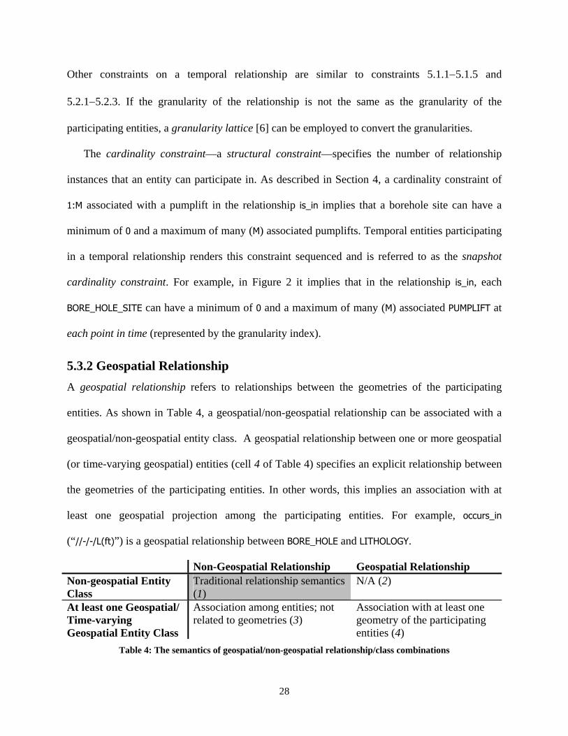
Other constraints on a temporal relationship are similar to constraints 5.1.1−5.1.5 and
5.2.1−5.2.3. If the granularity of the relationship is not the same as the granularity of the
participating entities, a granularity lattice [6] can be employed to convert the granularities.
The cardinality constraint—a structural constraint—specifies the number of relationship
instances that an entity can participate in. As described in Section 4, a cardinality constraint of
1:M associated with a pumplift in the relationship is_in implies that a borehole site can have a
minimum of 0 and a maximum of many (M) associated pumplifts. Temporal entities participating
in a temporal relationship renders this constraint sequenced and is referred to as the snapshot
cardinality constraint. For example, in Figure 2 it implies that in the relationship is_in, each
BORE_HOLE_SITE can have a minimum of 0 and a maximum of many (M) associated PUMPLIFT at
each point in time (represented by the granularity index).
5.3.2 Geospatial Relationship A geospatial relationship refers to relationships between the geometries of the participating
entities. As shown in Table 4, a geospatial/non-geospatial relationship can be associated with a
geospatial/non-geospatial entity class. A geospatial relationship between one or more geospatial
(or time-varying geospatial) entities (cell 4 of Table 4) specifies an explicit relationship between
the geometries of the participating entities. In other words, this implies an association with at
least one geospatial projection among the participating entities. For example, occurs_in
(“//-/-/L(ft)”) is a geospatial relationship between BORE_HOLE and LITHOLOGY.
Non-Geospatial Relationship Geospatial Relationship Non-geospatial Entity Class
Traditional relationship semantics (1)
N/A (2)
At least one Geospatial/ Time-varying Geospatial Entity Class
Association among entities; not related to geometries (3)
Association with at least one geometry of the participating entities (4)
Table 4: The semantics of geospatial/non-geospatial relationship/class combinations

29
While LITHOLOGY is a non-geospatial entity class, BORE_HOLE is a geospatial entity class. A
geospatial relationship means that different parts of a borehole (along the z-dimension) are
associated with different lithologies. Capturing this relationship would enable answering queries
like “What is the lithology at a depth of 50 feet of a specified borehole?” A non-geospatial
relationship between geospatial entities (cell 3 of Table 4) implies a relationship among entities
that is unrelated to its geometry. A geospatial relationship between non-geospatial entities (cell 2
of Table 4) is illegitimate as it contradicts the definition of a geospatial relationship, i.e., it is a
relationship between the geospatial projection of geospatial entities.
In this section, we outlined the semantics of annotations and how our annotation-based
approach naturally extends the semantics of a conventional conceptual model. Having described
the syntax (Section 3.4) and semantics (Section 5.1-5.3) of a geo-spatio-temporal conceptual
model, we apply our approach to the hydrogeologic application described in Section 2.
5.4 A Geo-spatio-temporal Application: Reprise Based on the temporal and geospatial requirements described in Section 2, the data analyst
captures the geo-spatio-temporal requirements of the user using annotations. At this time the data
analyst asks the application users questions like: Do you want to store the history or only the
current value of this fact? Do you want to capture the history of facts (valid time) or sequence of
updates (transaction time), or both? What is the associated temporal granularity? Does the fact
need to be modeled as an event or a state? Accordingly, the data analyst annotates the schema
shown in Figure 2 resulting in the annotated schema (or ST USM schema) shown in Figure 4.
Note how Figure 4 augments the schema shown in Figure 2 with geo-spatio-temporal
annotations. For example, SPRING needs to be represented as a region with horizontal geospatial
granularity of degree. The annotation phrase associated with the entity class SPRING is
“//R(deg)/R(deg)/-”.

30
GROUND_WATER_STATION
BORE_HOLESPRING
HOLE_INTERVAL
CASING
OPENING
PUMPLIFTis_in
station_name
Grp
occurs_in
LITHOLOGY
SOURCE_AGENCY
spring_measure Grp
WATER_LEVEL
bore_measure
S
serial_no
DISCHARGE
site_use
0:M1:1
1:M
1:M
0:M
type
opening_type
material
1:1
0:M
interval_ID
test
transmissivity
horizontal_conductivity
vertical_conductivity
leakance
diffusivity
storage
agency_code
tech_name
amount
source
method
water_depth
source
BORE_HOLE_SITE
SPRING_SITE
site_ID
improvement
diameter
site_ID
1:1
exists_in
1:1
0:M
covers
1:1
1:M
station_use
method
typedepth
mfg
construction_date
source
diameter
diameter
material
thickness
formation_name
permanence
remarks
discharge_duration
lithology_type
referencelithology_ID
status
opening_ID
casing_ID
statusdescription
IO_WATER_LEVEL
Enum
project
useflag
condition_flag
method
interpreter
IO_DISCHARGE
project
useflag
condition_flag
method
interpreter
Enum
calibration
altitude
equipment
type
type
age
erathem
system
series
ACCESS_TUBE
has
diameter
materialthickness
access_tube_ID
0:M
1:M
improvement
measuring_point
depth
weight
weight
discharge_ID
io_discharge_ID
water_level_ID
io_water_level_ID
bore_hole_ID
spring_ID
S(day)/-//P(deg)/P(deg)/-
S(min)/-//
S(day)/-//
E(min)/-//
E(min)/-//
S(min)/-//
E(day)/-//
E(day)/-//P(deg)/P(deg)/P(ft)
//P(deg)/P(deg)/L(ft)//R(deg)/R(deg)/-
//P(deg)/P(deg)/L(ft)
//-/-/L(ft)
//P(deg)/P(deg)/L(ft)
//P(deg)/P(deg)/L(ft)
S(day)/-//
Figure 4: An annotated schema (ST USM) for the ground-water flow model
The attribute test (of entity class BORE_HOLE_SITE) is a temporal attribute represented as an event
with temporal granularity of day. A borehole may have different lithology at different depths.
While LITHOLOGY is a non-geospatial entity class, BORE_HOLE is a geospatial entity class. The
occurs_in relationship is geospatial, associating LITHOLOGY to different depths of BORE_HOLE.
which is why the annotation for occurs_in is “//-/-/L(ft)”.
Since a translated USM schema for the complete ST USM schema in Figure 4 would be very
involved, we take a small portion of the ST USM schema (the grayed portion of Figure 4) and
present the explicated geo-spatio-temporal semantics via a translated USM schema in Figure 5.
Additionally, fifteen constraints—implicit in the ST USM schema in Figure 4—are associated
with the translated USM schema (shown in Figure 5) [15].

31
test
transmissivity
horizontal_conductivity
vertical_conductivity
leakance
diffusivity
storage
BORE_HOLE_SITE
site_ID
remarks
status
E(day)/-//
//P(deg)/P(deg)/P(ft)
test
transmissivity
horizontal_conductivity
vertical_conductivity
leakance
diffusivity
storage
BORE_HOLE_SITEsite_ID
remarks
status
VERTICAL_SPATIAL_GRANULARITY
HORIZONTAL_SPATIAL_GRANULARITY
TEMPORAL GRANULARITY
groups_into_xy
anchor_gran_xy
BORE_HOLE_SITE_xy_belongs_to
granularity_name
anchor extent
xy_minimumxy_maximum
groups_into_z
anchor_gran_z
0:1 0:M 0:M
0:M
0:M
0:M
0:M0:1
1:10:M
granularity_name
anchor extent
z_minimumz_maximum
BORE_HOLE_SITE_z_
belongs_to
0:M
1:1
BORE_HOLE_SITE_test_
REL
state_periodsstate_periods
BORE_HOLE_SITE_test
BORE_HOLE_SITE_test_
has_VT
0:M
1:1
groups_intoanchor_
gran
granularity_name
anchor extent
minimummaximum
0:1
0:M
0:M
0:M
ST USM
USM
geo
xy_point z_line
z_node_endz_node_start
z_line_points
1:1
0:1
bore_hole_site_test_ID
Figure 5: ST USM schema and its semantics using translated USM schema
In our geo-spatio-temporal conceptual design methodology, the annotated schemas capture
geo-spatio-temporal requirements of the users and validate their requirements. While the ST
USM schema succinctly encapsulates the geo-spatio-temporal data semantics, the translated
USM schema explicates the geo-spatio-temporal semantics in terms of the abstractions of a
conventional conceptual model and constraints expressed first-order logic. As shown by this
example, a few straightforward annotations capture the (quite complex) underlying geo-spatio-
temporal data semantics of the application.

32
Mapping rules provide correspondences between conceptual and logical model constructs
and are applied in logical design. Such a (logical) mapping depends on the geo-spatio-temporal
support provided by the logical model, which is outside the scope of this paper.
6 Evaluation We evaluate our proposed approach based on the criteria explicated in Section 2.2.
Expressiveness: We proposed intuitive ontology-based grammar for annotation that
comprehensively captures the semantics related to space and time.
Simplicity: With our approach, we have integrated the semantics of space and time into a
traditional conceptual model. Simplicity implies that (i) our approach is generic and can be
integrated into any conventional conceptual model [1, 3, 7]; (ii) the syntax is straightforward
to understand and use, as shown by a separate user study [14]; and (iii) our proposed
formalism, if adopted into an existing conceptual design tool (e.g., DISTIL [14]), would
require minimal changes to that tool.
Minimality: Since various types of conceptual modeling abstractions (e.g., entity, attribute,
relationship and key) are orthogonal to space and time, the annotations are minimal and
generic, i.e., applicable to all types of conceptual modeling abstractions.
Formality: We have defined the syntax formally in BNF (Figure 1) and used first-order logic
to define the semantics formally (cf. Section 5).
Upward compatibility: As our proposed extension is a strict superset provided by adding
non-mandatory semantics, the geo-spatio-temporal extension is upward compatible with the
conventional conceptual model.
Snapshot reducibility: Our annotation-based approach naturally extends the conventional
conceptual model without increasing complexity from the perspective of users, data analysts
and CASE (Computer-Aided Software/Systems Engineering) tool vendors.

33
With our annotation-based approach, we claim to have achieved comprehensiveness and
formality along with simplicity in geo-spatio-temporal conceptual modeling.
7 Summary Lee and Isdale [18] argue that there is a need for a special purpose conceptual model that is
suitable for GIS applications. Additionally, the proposed model of space and time needs to be
reconciled with the extant conceptual models developed in the database community [9].
A data semantics provide “a connection from a database to the real world outside the
database” [26] and a conceptual model provides a mechanism to capture the data semantics. In
this paper, we described an annotation-based approach for elicitation of the geo-spatio-temporal
semantics. While we posit that the spatio-temporal annotation presented in this paper is
comprehensive, it is impossible to assert completeness with conceptual modeling because any
formalism is motivated in part by pragmatic rather than purely theoretical reasons. It is possible
that the formalism presented in this paper may need to be extended for a geo-spatio-temporal
application, e.g., mobile transactions [12, 25]. In such a case, the annotations presented in this
paper can be easily extended. Since spatio-temporal annotations are orthogonal to the conceptual
modeling abstractions, our annotation-based approach is not only generic but also
straightforward to extend.
Further work would be useful in several areas. It would also be helpful to explore how
ST USM can be used as a canonical model for information integration of distributed geo-spatio-
temporal data. The annotations should be extended to incorporate schema versioning [24], as
well as to provide a mechanism for modeling geo-spatio-temporal constraints in a conceptual
schema, such as lifetime constraints and topological constraints. Finally, it will be useful to
explore how annotations can be applied to geo-spatio-temporal processes (STP) [4].
34
References [1] C. Batini, S. Ceri, and S. B. Navathe, Conceptual Database Design: An Entity-
Relationship Approach: Benjamin/Cummings Publishing Company, 1992. [2] M. H. Böhlen, C. S. Jensen, and R. T. Snodgrass, "Temporal Statement Modifiers," ACM
Transactions on Database Systems, vol. 25, No. 4, pp. 407-456, 2000. [3] P. P. Chen, "The Entity-Relationship Model - Toward a Unified View of Data," ACM
Transactions of Database Systems, vol. 1, No. 1, pp. 9-36, 1976. [4] C. Claramunt, C. Parent, and M. Thériault, "An Entity-relationship Model for Spatio-
Temporal Processes. DS-7 1997: 455-475," Data Mining and Reverse Engineering: Searching for Semantics, IFIP TC2/WG2.6 Seventh Conference on Database Semantics (DS-7), Leysin, Switzerland, pp. 455-475, 1997.
[5] F. A. D'Agnese, C. C. Faunt, A. K. Turner, and M. C. Hill, "Hydrogeologic evaluation and numerical simulation of the Death Valley Regional ground-water flow system, Nevada and California," U.S. Geological Survey Water Resources 96-4300, 1997.
[6] C. E. Dyreson, W. S. Evans, H. Lin, and R. T. Snodgrass, "Efficiently Supporting Temporal Granularities," IEEE Transactions on Knowledge and Data Engineering, vol. 12, No. 4, pp. 568-587, 2000.
[7] R. Elmasri and S. B. Navathe, Fundamentals of Database Systems, Second ed. Redwood City, CA: Benjamin/ Cummings Publishing Co., 1994.
[8] S. K. Gadia, "A Homogeneous Relational Model and Query Languages for Temporal Databases," ACM Transactions of Database Systems, vol. 13, No. 4, pp. 418-448, 1988.
[9] S. C. Guptill, "Multiple Representations of Geographic Entities Through Space and Time," Proceedings of the 4th International Symposium on Spatial Data Handling, Zurich, Switzerland, pp. 859-868, 1990.
[10] A. F. Hutchings and S. T. Knox, "Creating Products -- Customers Demand," Communications of the ACM, vol. 38, No. 5, pp. 72-80, 1995.
[11] C. S. Jensen, C. E. Dyreson, M. Bohlen, J. Clifford, R. Elmasri, S. K. Gadia, F. Grandi, P. Hayes, S. Jajodia, W. Kafer, N. Kline, N. Lorentzos, Y. Mitsopoulos, A. Montanari, D. Nonen, E. Peresi, B. Pernici, J. F. Roddick, N. L. Sarda, M. R. Scalas, A. Segev, R. T. Snodgrass, M. D. Soo, A. Tansel, R. Tiberio, and G. Wiederhold, "A Consensus Glossary of Temporal Database Concepts-February 1998 Version," in Temporal Databases: Research and Practice, O. Etzion, S. Jajodia, and S. Sripada, Eds.: Springer-Verlag, 1998.
[12] J. Jing, A. Helal, and A. K. Elmagarmid, "Client-Server Computing in Mobile Environments," ACM Computing Surveys, vol. 31, No. 2, pp. 117-157, 1999.
[13] S. Juhn and J. Naumann, "The Effectiveness of Data Representation Characteristics on User Validation," 6th International Conference on Information Systems, pp. 212-226, 1985.
[14] V. Khatri, "Bridging the Spatio-Temporal Semantic Gap: A Theoretical Framework, Evaluation and A Prototype System," in Doctoral Thesis: Management Information Systems Department. Tucson, AZ: University of Arizona, 2002, pp. 320.
[15] V. Khatri, S. Ram, and R. T. Snodgrass, "ST-USM: Bridging the Semantic Gap with a Spatio-temporal Conceptual Model," TimeCenter Technical Report TR-64, 2001.
[16] V. Khatri, S. Ram, and R. T. Snodgrass, "Supporting User-defined Granularities and Indeterminacy in a Spatiotemporal Conceptual Model," Annals of Mathematics and Artificial Intelligence, vol. 36, No. 1-2, pp. 195-232, 2002.

35
[17] B. Kuipers, "Modeling Spatial Knowledge," Cognitive Science, vol. 2, pp. 129-153, 1978. [18] Y. C. Lee and M. Isdale, "The Need for a Spatial Data Model," Canadian Conference in
GIS-911991. [19] D. M. Mark and A. U. Frank, "Experiential and Formal Models of Geographic Space,"
Environment and Planning, vol. 23, No. 1, pp. 3-24, 1996. [20] J. L. Mennis, D. J. Peuquet, and L. Qian, "A Conceptual Framework for Incorporating
Cognitive Principles into Geographical Database Representation," International Journal of Geographic Information Science, vol. 14, No. 6, pp. 501-520, 2000.
[21] D. J. Peuquet, "It's about Time: A Conceptual Framework for the Representation of Temporal Dynamics in Geographic Information Systems," Annals of the Association of American Geographers, vol. 83, No. 3, pp. 441-461, 1994.
[22] S. Ram, "Intelligent Database Design using the Unifying Semantic Model," Information and Management, vol. 29, No. 4, pp. 191-206, 1995.
[23] C. V. Ramamoorthy, A. Prakash, W. Tsai, and Y. Usuda, "Software Engineering: Problems and Perspectives," Computer, vol. 17, No. 10, pp. 191-209, 1984.
[24] J. F. Roddick and R. T. Snodgrass, "Schema Versioning," in The TSQL2 Temporal Query Language, R. T. Snodgrass, Ed. Boston: Kluwer Academic Publishers, 1995, pp. 427-449.
[25] P. Serrano-Alvarado, C. Roncancio, and M. E. Adiba, "Analyzing Mobile Transaction Supports for DBMS," 12th International Workshop on Database and Expert Systems Applications (DEXA 2001), Munich, Germany, pp. 595-600, 2001.
[26] A. Sheth, "Data Semantics: What, Where and How?," 6th IFIP Working Conference on Data Semantics (DS-6), Atlanta, Georgia, pp. 601-610, 1995.
[27] A. Silbershatz, H. Korth, and S. Sudarshan, Database System Concepts, Third Edition ed: WCB/ McGraw Hill, 1997.
[28] R. T. Snodgrass and I. Ahn, "Temporal Databases," IEEE Computer, vol. 19, No. 9, pp. 35-42, 1986.
[29] N. Tryfona and C. S. Jensen, "Conceptual Data Modeling for Spatiotemporal Applications," Geoinformatica, vol. 3, No. 3, pp. 245-268, 1999.
[30] J. W. van Roessel, "Design of a Spatial Data Structure using the Relational Normal Form," International Journal of Geographical Information Systems, vol. 1, No. 1, pp. 33-50, 1987.
[31] Y. Wand, D. E. Monarchi, J. Parsons, and C. C. Woo, "Theoretical Foundations for Conceptual Modeling in Information Systems Development," Decision Support Systems, vol. 15, No. 4, pp. 285-304, 1995.
[32] Y. Wand, V. C. Storey, and R. Weber, "On Ontological Analysis of the Relationship Construct in Conceptual Modeling," ACM Transactions of Database Systems, vol. 24, No. 4, pp. 494-528, 1999.
[33] M. F. Worboys, H. M. Hearshaw, and D. J. Maguire, "Object-oriented data modeling for spatial databases," International Journal of Geographical Information Systems, vol. 4, No. 4, pp. 369-383, 1990.