Embed Size (px)
Citation preview
Auditory-Based Noise-Robust AudioClassification Algorithms
Wei Chu
Department of Electrical & Computer EngineeringMcGill UniversityMontreal, Canada
September 2008
A thesis submitted to McGill University in partial fulfillment of the requirements for thedegree of Doctor of Philosophy.
c© 2008 Wei Chu
i
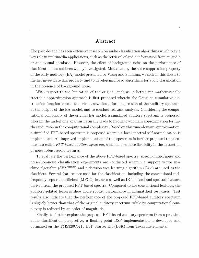
Abstract
The past decade has seen extensive research on audio classification algorithms which play a
key role in multimedia applications, such as the retrieval of audio information from an audio
or audiovisual database. However, the effect of background noise on the performance of
classification has not been widely investigated. Motivated by the noise-suppression property
of the early auditory (EA) model presented by Wang and Shamma, we seek in this thesis to
further investigate this property and to develop improved algorithms for audio classification
in the presence of background noise.
With respect to the limitation of the original analysis, a better yet mathematically
tractable approximation approach is first proposed wherein the Gaussian cumulative dis-
tribution function is used to derive a new closed-form expression of the auditory spectrum
at the output of the EA model, and to conduct relevant analysis. Considering the compu-
tational complexity of the original EA model, a simplified auditory spectrum is proposed,
wherein the underlying analysis naturally leads to frequency-domain approximation for fur-
ther reduction in the computational complexity. Based on this time-domain approximation,
a simplified FFT-based spectrum is proposed wherein a local spectral self-normalization is
implemented. An improved implementation of this spectrum is further proposed to calcu-
late a so-called FFT-based auditory spectrum, which allows more flexibility in the extraction
of noise-robust audio features.
To evaluate the performance of the above FFT-based spectra, speech/music/noise and
noise/non-noise classification experiments are conducted wherein a support vector ma-
chine algorithm (SVMstruct) and a decision tree learning algorithm (C4.5) are used as the
classifiers. Several features are used for the classification, including the conventional mel-
frequency cepstral coefficient (MFCC) features as well as DCT-based and spectral features
derived from the proposed FFT-based spectra. Compared to the conventional features, the
auditory-related features show more robust performance in mismatched test cases. Test
results also indicate that the performance of the proposed FFT-based auditory spectrum
is slightly better than that of the original auditory spectrum, while its computational com-
plexity is reduced by an order of magnitude.
Finally, to further explore the proposed FFT-based auditory spectrum from a practical
audio classification perspective, a floating-point DSP implementation is developed and
optimized on the TMS320C6713 DSP Starter Kit (DSK) from Texas Instruments.
ii
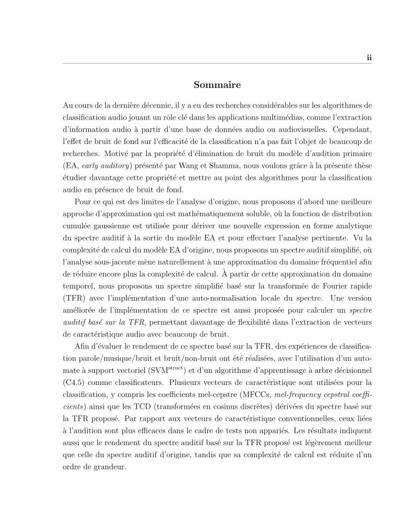
Sommaire
Au cours de la derniere decennie, il y a eu des recherches considerables sur les algorithmes de
classification audio jouant un role cle dans les applications multimedias, comme l’extraction
d’information audio a partir d’une base de donnees audio ou audiovisuelles. Cependant,
l’effet de bruit de fond sur l’efficacite de la classification n’a pas fait l’objet de beaucoup de
recherches. Motive par la propriete d’elimination de bruit du modele d’audition primaire
(EA, early auditory) presente par Wang et Shamma, nous voulons grace a la presente these
etudier davantage cette propriete et mettre au point des algorithmes pour la classification
audio en presence de bruit de fond.
Pour ce qui est des limites de l’analyse d’origine, nous proposons d’abord une meilleure
approche d’approximation qui est mathematiquement soluble, ou la fonction de distribution
cumulee gaussienne est utilisee pour deriver une nouvelle expression en forme analytique
du spectre auditif a la sortie du modele EA et pour effectuer l’analyse pertinente. Vu la
complexite de calcul du modele EA d’origine, nous proposons un spectre auditif simplifie, ou
l’analyse sous-jacente mene naturellement a une approximation du domaine frequentiel afin
de reduire encore plus la complexite de calcul. A partir de cette approximation du domaine
temporel, nous proposons un spectre simplifie base sur la transformee de Fourier rapide
(TFR) avec l’implementation d’une auto-normalisation locale du spectre. Une version
amelioree de l’implementation de ce spectre est aussi proposee pour calculer un spectre
auditif base sur la TFR, permettant davantage de flexibilite dans l’extraction de vecteurs
de caracteristique audio avec beaucoup de bruit.
Afin d’evaluer le rendement de ce spectre base sur la TFR, des experiences de classifica-
tion parole/musique/bruit et bruit/non-bruit ont ete realisees, avec l’utilisation d’un auto-
mate a support vectoriel (SVMstruct) et d’un algorithme d’apprentissage a arbre decisionnel
(C4.5) comme classificateurs. Plusieurs vecteurs de caracteristique sont utilisees pour la
classification, y compris les coefficients mel-cepstre (MFCCs, mel-frequency cepstral coeffi-
cients) ainsi que les TCD (transformees en cosinus discretes) derivees du spectre base sur
la TFR propose. Par rapport aux vecteurs de caracteristique conventionnelles, ceux liees
a l’audition sont plus efficaces dans le cadre de tests non apparies. Les resultats indiquent
aussi que le rendement du spectre auditif base sur la TFR propose est legerement meilleur
que celle du spectre auditif d’origine, tandis que sa complexite de calcul est reduite d’un
ordre de grandeur.
iii
Enfin, pour explorer davantage le spectre auditif base sur la TFR propose d’un point
de vue de classification audio pratique, une implementation de traitement numerique du
signal en virgule flottante est mise au point et optimisee grace au necessaire de demarrage
pour le traitement de signal numerique (DSK, DSP Starter Kit) TMS320C6713 de Texas
Instruments.
iv
Acknowledgments
I would like to express my deepest gratitude to my supervisor, Professor Benoıt Champagne,
for his guidance, encouragement and support throughout the course of my Ph.D. studies.
I am grateful for the financial support from Professor Champagne via research grants from
the Natural Sciences and Engineering Research Council of Canada (NSERC).
Many thanks are extended to Professor Douglas O’Shaughnessy and Professor Jeremy
R. Cooperstock, members of my Ph.D. committee, for their feedback and suggestions.
I would also like to thank my external examiner, Professor Pierre Dumouchel of Ecole
de technologie superieure, and the members of my defence committee, namely: Professor
M. Dobbs, Professor F. Labeau, Professor B. Champagne, Professor J. Clark, Prof. D.
O’Shaughnessy, and Professor W. Zhu of Concordia University, for their valuable comments
and suggestions.
During my stay at McGill, I have met many dedicated students, faculty and staff mem-
bers who have made my Ph.D. studies a memorable experience. In particular, I am grateful
to my fellow graduate students in the Telecommunications and Signal Processing (TSP)
Laboratory, and especially to Eric Plourde and Rui Ma, for their friendship, support, and
help. My special thanks go to Eric for his help with the French-version abstract of the
thesis.
I am deeply indebted to my parents, parents-in-law, sister and other family members
for their love and support. Last but not least, my deepest gratitude goes to my wife, Yong
Hong, for her unconditional love, support, understanding, and patience throughout my
studies.
v
Contents
1 Introduction 1
1.1 Content-Based Audio Analysis . . . . . . . . . . . . . . . . . . . . . . . . . 1
1.2 Motivation and Research Objective . . . . . . . . . . . . . . . . . . . . . . 5
1.3 Main Contributions . . . . . . . . . . . . . . . . . . . . . . . . . . . . . . . 8
1.3.1 Extended Analysis of Self-Normalization . . . . . . . . . . . . . . . 9
1.3.2 Simplification/Approximation of the Auditory Spectrum . . . . . . 9
1.3.3 Setup of the Audio Classification Experiment . . . . . . . . . . . . 10
1.3.4 DSP Demo System . . . . . . . . . . . . . . . . . . . . . . . . . . . 10
1.3.5 Publications . . . . . . . . . . . . . . . . . . . . . . . . . . . . . . . 11
1.4 Thesis Organization . . . . . . . . . . . . . . . . . . . . . . . . . . . . . . . 11
2 A Review of Audio Classification Algorithms 13
2.1 Audio Signals . . . . . . . . . . . . . . . . . . . . . . . . . . . . . . . . . . 14
2.1.1 Speech and Music Classification . . . . . . . . . . . . . . . . . . . . 14
2.1.2 Environmental Sound and Background Noise . . . . . . . . . . . . . 15
2.1.3 Use of Compressed Audio Data . . . . . . . . . . . . . . . . . . . . 17
2.2 Audio Features . . . . . . . . . . . . . . . . . . . . . . . . . . . . . . . . . 18
2.2.1 Frame-Level Features . . . . . . . . . . . . . . . . . . . . . . . . . . 18
2.2.2 Clip-Level Features . . . . . . . . . . . . . . . . . . . . . . . . . . . 25
2.3 Classification Methods . . . . . . . . . . . . . . . . . . . . . . . . . . . . . 28
2.3.1 Gaussian Mixture Model . . . . . . . . . . . . . . . . . . . . . . . . 29
2.3.2 Hidden Markov Model . . . . . . . . . . . . . . . . . . . . . . . . . 29
2.3.3 Support Vector Machine . . . . . . . . . . . . . . . . . . . . . . . . 31
2.3.4 Nearest Neighbor . . . . . . . . . . . . . . . . . . . . . . . . . . . . 33
Contents vi
2.3.5 Neural Network . . . . . . . . . . . . . . . . . . . . . . . . . . . . . 34
2.3.6 Linear Discriminant Analysis . . . . . . . . . . . . . . . . . . . . . 35
2.3.7 Other Classification Approaches . . . . . . . . . . . . . . . . . . . . 35
2.4 Conclusion . . . . . . . . . . . . . . . . . . . . . . . . . . . . . . . . . . . . 36
3 Early Auditory Model and the Noise-Suppression Property 38
3.1 Structure of the EA Model . . . . . . . . . . . . . . . . . . . . . . . . . . . 39
3.2 Noise-Suppression Property . . . . . . . . . . . . . . . . . . . . . . . . . . 41
3.2.1 Qualitative Analysis . . . . . . . . . . . . . . . . . . . . . . . . . . 41
3.2.2 Quantitative Analysis of a Special Case . . . . . . . . . . . . . . . . 43
3.3 Audio Classification using EA Model-Based Features . . . . . . . . . . . . 43
3.4 Open Research Problems . . . . . . . . . . . . . . . . . . . . . . . . . . . . 45
3.5 Conclusion . . . . . . . . . . . . . . . . . . . . . . . . . . . . . . . . . . . . 46
4 Analysis of the Self-Normalization Property 48
4.1 Gaussian CDF and Sigmoid Compression Function . . . . . . . . . . . . . 48
4.2 Closed-Form Expression of E[y4(t, s)] . . . . . . . . . . . . . . . . . . . . . 50
4.3 Local Spectral Enhancement . . . . . . . . . . . . . . . . . . . . . . . . . . 51
4.4 Approximation using a Gaussian Mixture Function . . . . . . . . . . . . . 53
4.5 Conclusion . . . . . . . . . . . . . . . . . . . . . . . . . . . . . . . . . . . . 54
5 Simplification of the Auditory Spectrum 56
5.1 Time-Domain Simplified Auditory Spectrum . . . . . . . . . . . . . . . . . 57
5.1.1 Nonlinear Compression . . . . . . . . . . . . . . . . . . . . . . . . . 57
5.1.2 Half-Wave Rectification and Temporal Integration . . . . . . . . . . 57
5.1.3 Simplified Auditory Spectrum . . . . . . . . . . . . . . . . . . . . . 57
5.2 Implementation 1: A FFT-Based Self-Normalized Spectrum . . . . . . . . 59
5.2.1 Normalization of the Input Signal . . . . . . . . . . . . . . . . . . . 59
5.2.2 Calculation of a Short-Time Power Spectrum . . . . . . . . . . . . 60
5.2.3 Power Spectrum Grouping . . . . . . . . . . . . . . . . . . . . . . . 60
5.2.4 Spectral Self-Normalization . . . . . . . . . . . . . . . . . . . . . . 61
5.2.5 Post-Processing . . . . . . . . . . . . . . . . . . . . . . . . . . . . . 62
5.3 Implementation 2: A FFT-Based Auditory Spectrum . . . . . . . . . . . . 62
5.3.1 Normalization of the Input Signal . . . . . . . . . . . . . . . . . . . 63
Contents vii
5.3.2 Calculation of a Short-Time Power Spectrum . . . . . . . . . . . . 63
5.3.3 Power Spectrum Selecting . . . . . . . . . . . . . . . . . . . . . . . 63
5.3.4 Spectral Self-Normalization . . . . . . . . . . . . . . . . . . . . . . 64
5.3.5 Post-Processing . . . . . . . . . . . . . . . . . . . . . . . . . . . . . 68
5.4 Conclusion . . . . . . . . . . . . . . . . . . . . . . . . . . . . . . . . . . . . 69
6 Audio Classification Experiments 70
6.1 Audio Sample Database . . . . . . . . . . . . . . . . . . . . . . . . . . . . 70
6.1.1 16-kHz Samples . . . . . . . . . . . . . . . . . . . . . . . . . . . . . 70
6.1.2 8-kHz Samples . . . . . . . . . . . . . . . . . . . . . . . . . . . . . 71
6.1.3 Pre-Processing of Audio Samples . . . . . . . . . . . . . . . . . . . 73
6.1.4 Testing Approach . . . . . . . . . . . . . . . . . . . . . . . . . . . . 75
6.2 Audio Features . . . . . . . . . . . . . . . . . . . . . . . . . . . . . . . . . 75
6.2.1 MFCC Features . . . . . . . . . . . . . . . . . . . . . . . . . . . . . 76
6.2.2 Spectral Features . . . . . . . . . . . . . . . . . . . . . . . . . . . . 76
6.2.3 DCT-Based Features . . . . . . . . . . . . . . . . . . . . . . . . . . 78
6.2.4 Clip-Level Features . . . . . . . . . . . . . . . . . . . . . . . . . . . 79
6.3 Implementation . . . . . . . . . . . . . . . . . . . . . . . . . . . . . . . . . 84
6.3.1 NSL Matlab Toolbox . . . . . . . . . . . . . . . . . . . . . . . . . . 84
6.3.2 Classification Approaches . . . . . . . . . . . . . . . . . . . . . . . 84
6.4 Performance Analysis . . . . . . . . . . . . . . . . . . . . . . . . . . . . . . 86
6.4.1 Performance Comparison with the 16-kHz Database . . . . . . . . . 86
6.4.2 Performance Comparison with the 8-kHz Database . . . . . . . . . 92
6.4.3 Effect of Running Average Coefficients . . . . . . . . . . . . . . . . 94
6.4.4 Computational Complexity . . . . . . . . . . . . . . . . . . . . . . . 94
6.5 Conclusion . . . . . . . . . . . . . . . . . . . . . . . . . . . . . . . . . . . . 95
7 Implementation Based on TMS320C6713 DSK 97
7.1 Implementation of the Proposed Audio Classification Algorithm . . . . . . 98
7.1.1 Structure of the System . . . . . . . . . . . . . . . . . . . . . . . . 98
7.1.2 Tracing the Computational Complexity . . . . . . . . . . . . . . . . 102
7.2 Analysis of the Complexity . . . . . . . . . . . . . . . . . . . . . . . . . . . 105
7.2.1 Initial Implementation . . . . . . . . . . . . . . . . . . . . . . . . . 105
Contents viii
7.2.2 Compiler Optimization . . . . . . . . . . . . . . . . . . . . . . . . . 106
7.2.3 Optimization of DCT and FFT Modules . . . . . . . . . . . . . . . 109
7.2.4 Use of C67x FastRTS Optimized Library . . . . . . . . . . . . . . . 112
7.3 Conclusion . . . . . . . . . . . . . . . . . . . . . . . . . . . . . . . . . . . . 113
8 Summary and Conclusion 116
8.1 Summary of the Work . . . . . . . . . . . . . . . . . . . . . . . . . . . . . 116
8.2 Future Research . . . . . . . . . . . . . . . . . . . . . . . . . . . . . . . . . 119
A Closed-Form Expression of E[y4(t, s)] 122
B TMS320C6713 DSK 125
B.1 Hardware Overview . . . . . . . . . . . . . . . . . . . . . . . . . . . . . . . 125
B.2 Software Overview . . . . . . . . . . . . . . . . . . . . . . . . . . . . . . . 128
B.2.1 Code Creation . . . . . . . . . . . . . . . . . . . . . . . . . . . . . . 128
B.2.2 Debug . . . . . . . . . . . . . . . . . . . . . . . . . . . . . . . . . . 129
B.2.3 Analysis . . . . . . . . . . . . . . . . . . . . . . . . . . . . . . . . . 130
References 132
ix
List of Figures
1.1 Schematic description of an audio classification system. . . . . . . . . . . . 3
1.2 Schematic description of the EA model presented by Wang and Shamma
[WS94]. . . . . . . . . . . . . . . . . . . . . . . . . . . . . . . . . . . . . . 7
2.1 Spectral centroid. (a) Speech. (b) Music. (c) Noise. . . . . . . . . . . . . . 22
2.2 Linear separating hyperplane for a separable case. The support vectors are
circled. . . . . . . . . . . . . . . . . . . . . . . . . . . . . . . . . . . . . . . 31
3.1 Schematic description of the EA model [WS94]. . . . . . . . . . . . . . . . 39
4.1 Sigmoid function (α = 0.1) and Gaussian distribution function (σg = 0.163).
(a) g(x) and Φ (x/σg). (b) g′(x) and (1/σg)Φ′ (x/σg). . . . . . . . . . . . . 49
4.2 E[y4(t, s)] as a function of σu and σv. . . . . . . . . . . . . . . . . . . . . . 52
4.3 Sigmoid function (α = 0.1) and Gaussian mixture function (M = 4). . . . 54
5.1 Auditory spectrograms of a one-second speech clip. (a) Original auditory
spectrogram. (b) Simplified auditory spectrogram. (c) Simplified auditory
spectrogram without time-domain derivative. . . . . . . . . . . . . . . . . . 58
5.2 Schematic description of the proposed FFT-based implementations. . . . . 59
5.3 The cochlear filter H(ω, s) centered at 1017 Hz and the corresponding dif-
ferential filter ∂sH(ω, s) [Neu]. (The 3-dB bandwidth of the cochlear filter
is about 220 Hz, while the 3-dB bandwidth of the differential filter is 80 Hz.) 66
5.4 The filtering characteristics of the proposed running average scheme. . . . 67
5.5 Running average results. . . . . . . . . . . . . . . . . . . . . . . . . . . . . 67
5.6 A power spectrum vector and the corresponding self-normalized version. (a)
Whole data set. (b) Details of some spectral valleys. . . . . . . . . . . . . . 68
List of Figures x
5.7 The proposed FFT-based auditory spectrograms of a one-second speech clip.
(a) Clean case. (b) SNR = 15 dB (babble noise). (c) SNR = 15 dB (white
noise). . . . . . . . . . . . . . . . . . . . . . . . . . . . . . . . . . . . . . . 69
6.1 Structure of the VAD algorithms in [CAS05]. . . . . . . . . . . . . . . . . . 74
6.2 Characteristic frequency values corresponding to the index values i given in
Table 5.1. . . . . . . . . . . . . . . . . . . . . . . . . . . . . . . . . . . . . 78
6.3 Distributions of conventional MFCC features. For all figures, horizontal and
vertical axes refer to the variance values of the first and the second compo-
nents of the frame-level features respectively. (a)Speech (clean). (b)Music
(clean). (c)Noise. (d)Speech (SNR = 20 dB). (e)Speech (SNR = 15 dB).
(f)Speech (SNR = 10 dB). (g)Music (SNR = 20 dB). (h)Music (SNR = 15
dB). (i)Music (SNR = 10 dB). . . . . . . . . . . . . . . . . . . . . . . . . . 81
6.4 Distributions of DCT-based features obtained from original auditory spec-
trum. For all figures, horizontal and vertical axes refer to the variance values
of the first and the second components of the frame-level features respec-
tively. (a)Speech (clean). (b)Music (clean). (c)Noise. (d)Speech (SNR = 20
dB). (e)Speech (SNR = 15 dB). (f)Speech (SNR = 10 dB). (g)Music (SNR
= 20 dB). (h)Music (SNR = 15 dB). (i)Music (SNR = 10 dB). . . . . . . . 82
6.5 Distributions of DCT-based features obtained from FFT-based auditory
spectrum. For all figures, horizontal and vertical axes refer to the variance
values of the first and the second components of the frame-level features re-
spectively. (a)Speech (clean). (b)Music (clean). (c)Noise. (d)Speech (SNR
= 20 dB). (e)Speech (SNR = 15 dB). (f)Speech (SNR = 10 dB). (g)Music
(SNR = 20 dB). (h)Music (SNR = 15 dB). (i)Music (SNR = 10 dB). . . . 83
6.6 NSL toolbox GUI. . . . . . . . . . . . . . . . . . . . . . . . . . . . . . . . 84
6.7 Speech/music/noise classification error rates as a function of SNR for differ-
ent audio features (refer to Table 6.3). (a) SVM. (b) C4.5. . . . . . . . . . 87
7.1 Modules of the algorithm. (a) Frame-based processing. (b) Clip-based pro-
cessing. . . . . . . . . . . . . . . . . . . . . . . . . . . . . . . . . . . . . . . 100
7.2 The structure of a pipe [Tex04b]. . . . . . . . . . . . . . . . . . . . . . . . 101
7.3 Host Channel Control window. . . . . . . . . . . . . . . . . . . . . . . . . . 103
7.4 Statistics View window. . . . . . . . . . . . . . . . . . . . . . . . . . . . . 104
List of Figures xi
7.5 Audio classification decisions for a sample of 3 min long. There are 6 error
decisions out of a total of 180 decisions. . . . . . . . . . . . . . . . . . . . . 106
B.1 TMS320C6713 DSK block diagram [Spe04]. . . . . . . . . . . . . . . . . . 126
B.2 TMS320C6713 DSP core functional block diagram [Tex05c] . . . . . . . . . 127
xii
List of Tables
3.1 Error classification rates from [RA04] (%) . . . . . . . . . . . . . . . . . . 44
5.1 Frequency index values of Nk and φi . . . . . . . . . . . . . . . . . . . . . 65
6.1 Selected noise samples from the NOISEX database . . . . . . . . . . . . . 72
6.2 Selected noise samples from the IS-727 database . . . . . . . . . . . . . . . 73
6.3 Summary of the clip-level audio features . . . . . . . . . . . . . . . . . . . 79
6.4 Speech/music/noise classification error rates with a clean set as the training
data (%) . . . . . . . . . . . . . . . . . . . . . . . . . . . . . . . . . . . . . 88
6.5 Average classification error rates from cross-validation (%) . . . . . . . . . 90
6.6 Confusion matrices for different audio feature sets at SNR = 10 dB . . . . 91
6.7 Speech/music/noise classification error rates with a 15-dB set as the training
data (%) . . . . . . . . . . . . . . . . . . . . . . . . . . . . . . . . . . . . . 92
6.8 Noise/non-noise classification error rates with SVM as the classifier (%) . . 93
6.9 Error classification rates of the DCT-FFT2 features with different running
average coefficients (%) . . . . . . . . . . . . . . . . . . . . . . . . . . . . . 94
7.1 Size of the executable file . . . . . . . . . . . . . . . . . . . . . . . . . . . . 105
7.2 Computational complexity after introducing compiler optimization options 108
7.3 Reduction in the computational complexity after introducing optimizations
to DCT and FFT modules . . . . . . . . . . . . . . . . . . . . . . . . . . . 111
7.4 Reduction in computational complexity after using the FastRTS library . . 113
7.5 Size of the executable file after introducing all proposed optimizations . . . 113
xiii
List of Acronyms
AAC Advanced Audio Coding
ACC Average Computational Complexity
AI Artificial Intelligence
AMDF Average Magnitude Difference Function
ANN Artificial neural networks
ANSI American National Standards Institute
API Application Programming Interface
ASR Automatic Speech Recognition
ASB Audio Spectrum Basis
ASP Audio Spectrum Projection
BM Basilar Membrane
BP Band Periodicity
BSL Board Support Library
CCR Correct Classification Rate
CCStudio/CCS Code Composer Studio
CELP Code-Excited Linear Prediction
CF Characteristic Frequency
CPLD Complex Programmable Logic Device
CSL Chip Support Library
DCT Discrete Cosine Transform
DFT Discrete Fourier Transform
DIP Dual In-line Package
DIT Decimation In Time
DSK DSP Starter Kit
List of Terms xiv
DSP Digital Signal Processor or Digital Signal Processing
EAM Early Auditory Model
EDMA Enhanced Direct-Memory-Access
EM Expectation-Maximization
EMIF External Memory Interface
FFT Fast Fourier Transform
GMM Gaussian Mixture Model
GPIO General-Purpose Input/Output
GUI Graphical User Interface
HMM Hidden Markov Model
HOSVD Higher Order Singular Value Decomposition
HPI Host-Port Interface
HWR Half-Wave Rectification
HZCRR High Zero-Crossing Rate Ratio
I2C Inter-Integrated Circuit
IDE Integrated Development Environment
JTAG Joint Test Action Group
KNN K-Nearest-Neighbor
LDA Linear Discriminant Analysis
LED Light-Emitting Diode
LIN Lateral Inhibitory Network
LPC Linear Predictive Coding
LPCC Linear Prediction Coefficient-derived Cepstrum Coefficients
LP-ZCR Linear Prediction Zero-Crossing Ratio
LSF Line Spectrum Frequency
LSP Line Spectrum Pair
LSTER Low Short-Time Energy Ratio
McASP Multichannel Audio Serial Port
McBSP Multichannel Buffered Serial Port
MCC Maximum Computational Complexity
MDCT Modified Discrete Cosine Transform
MFCC Mel-Frequency Cepstral Coefficient
MFLOPS Million Floating-point Operations Per Second
List of Terms xv
MIPS Million Instructions Per Second
MMACS Million Multiply-Accumulate Operations Per Second
MP3 MPEG-1/MPEG-2 Audio Layer 3
MPEG Moving Picture Experts Group
NFL Nearest Feature Line
NFR Noise Frame Ratio
NRAF Noise-Robust Auditory Feature
PCA Principal Component Analysis
PCM Pulse Code Modulation
PLL Phase-Locked Loop
RMS Root Mean Square
RTA Real-Time Analysis
RTDX Real-Time Data Exchange
SFuF Short-Time Fundamental Frequency
SNR Signal-to-Noise Ratio
STRF Spectro-Temporal Response Field
SVM Support Vector Machine
TDMA Time Division Multiple Access
VLIW Very-Long-Instruction-Word
VoIP Voice over IP
ZCR Zero-Crossing Rate

List of Terms xvi
1
Chapter 1
Introduction
Today digital multimedia information has become a ubiquitous component of our lives.
Among these multimedia data, audio sequences constitute an important part. The expo-
nential growth of internet usage, the rapid increase in the speed and capacity of modern
computers, and the latest advances in network-related technologies have boosted appli-
cations of multimedia services which comprise audio elements, for example, voice-over-IP
(VoIP), on-line music sales, cellular telephony, simultaneous digital transmissions of live
television/radio station outputs, etc.
In many cases, the success of distributing audio data or providing client services compris-
ing audio data is greatly dependent on the ability to classify and retrieve audio information
in terms of their properties or contents. However, a raw audio signal data set is a large
featureless collection of bytes and does not readily allow content-based audio classification
and retrieval. It is thus desirable that certain signal processing approaches be explored
which allow efficient and automated content-based analysis for stored or streamed audio
data.
Below, the concept of content-based audio analysis is introduced first, followed by mo-
tivation and objective of the proposed research, and a summary of the main contributions.
Finally, an overview of this thesis is given.
1.1 Content-Based Audio Analysis
Considering the diversity of audio signals, in some applications it would be desirable to
classify audio clips in terms of their contents before other processing steps are further
1 Introduction 2
applied. For example, a speech/non-speech classifier is required if an automatic speech
recognition (ASR) unit is expected to be turned on for pure speech data only. In some cases,
people may benefit from isolating or retrieving any sound clips from an audio database,
wherein these clips could match a given excerpt or given properties. For low bit-rate
audio coding algorithms, to trade off audio quality against the average bit rate, a multi-
mode codec is often designed which can accommodate different signals. For example, in
[Qia97] and [TRRL00], the coding module is selected based on the output of a speech/music
classifier.
An audio signal clip is usually taken as a collection of bytes with only some common
information attached such as the name, format, sampling rate, size, etc. Clearly, the
attached information does not readily allow content-based analysis like classification or
retrieval. Searching for a particular audio class, such as applause, music played by a
violin, sound of a train, speech, or the speech of a particular speaker, can be a tedious
or even impossible task due to the inability to look inside the audio data. For a limited
amount of audio and video data, it is possible to create content-based information manually
for browsing and management. However, due to the rapid development in technologies
for data compression, storage, and transmission, the size of multimedia data collections
is increasing so fast, making manual indexing no longer appropriate. Besides, an index
information created manually by one person is highly subjective and may be of limited
use to another person. Therefore, a computer-based analysis of the semantic meanings of
the documents containing audio sequences, or video sequences with accompanying audio
tracks, is indispensable.
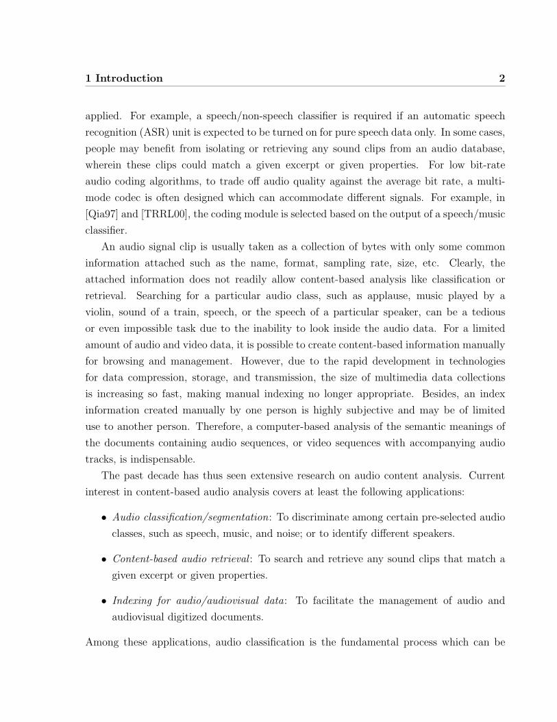
The past decade has thus seen extensive research on audio content analysis. Current
interest in content-based audio analysis covers at least the following applications:
• Audio classification/segmentation: To discriminate among certain pre-selected audio
classes, such as speech, music, and noise; or to identify different speakers.
• Content-based audio retrieval : To search and retrieve any sound clips that match a
given excerpt or given properties.
• Indexing for audio/audiovisual data: To facilitate the management of audio and
audiovisual digitized documents.
Among these applications, audio classification is the fundamental process which can be
1 Introduction 3
Pre- Processing
Feature Extraction
Audio Clip
Classifica- tion
Post- Processing
Audio Class
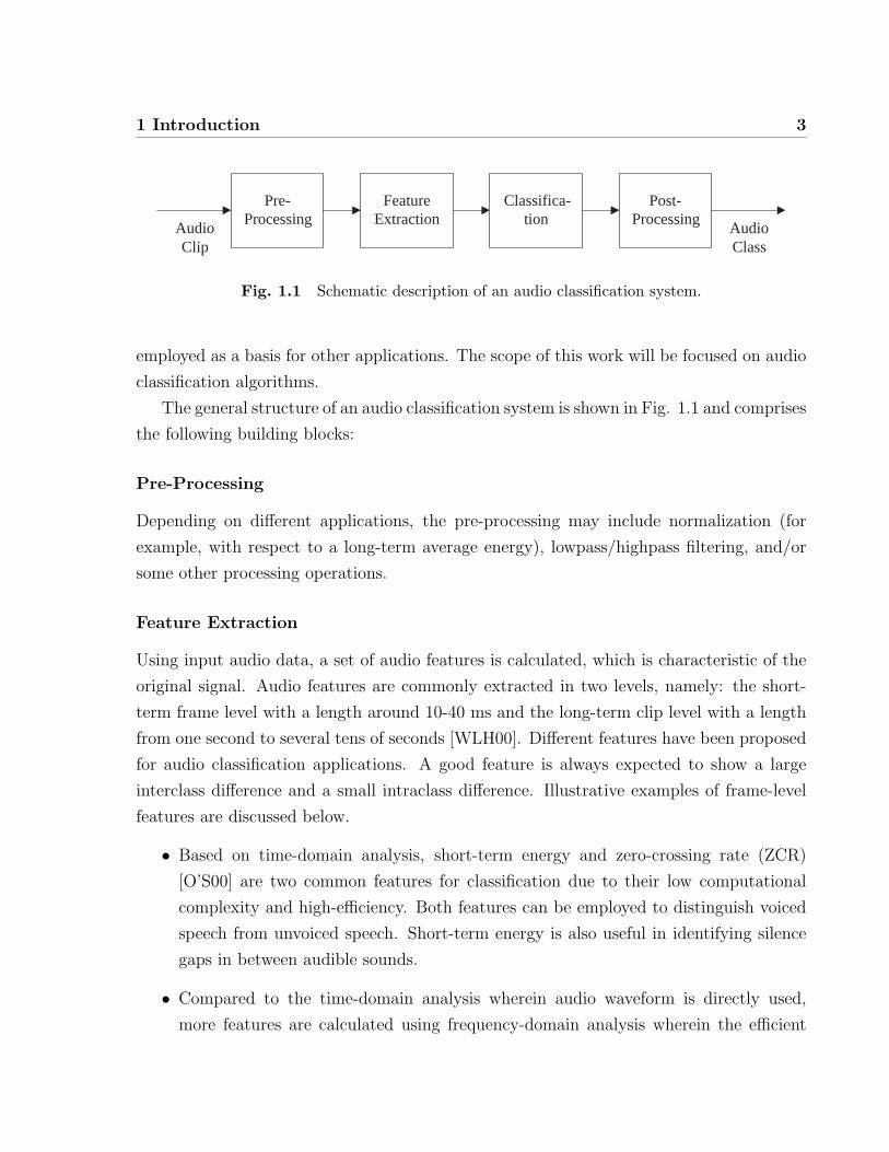
Fig. 1.1 Schematic description of an audio classification system.
employed as a basis for other applications. The scope of this work will be focused on audio
classification algorithms.
The general structure of an audio classification system is shown in Fig. 1.1 and comprises
the following building blocks:
Pre-Processing
Depending on different applications, the pre-processing may include normalization (for
example, with respect to a long-term average energy), lowpass/highpass filtering, and/or
some other processing operations.
Feature Extraction
Using input audio data, a set of audio features is calculated, which is characteristic of the
original signal. Audio features are commonly extracted in two levels, namely: the short-
term frame level with a length around 10-40 ms and the long-term clip level with a length
from one second to several tens of seconds [WLH00]. Different features have been proposed
for audio classification applications. A good feature is always expected to show a large
interclass difference and a small intraclass difference. Illustrative examples of frame-level
features are discussed below.
• Based on time-domain analysis, short-term energy and zero-crossing rate (ZCR)
[O’S00] are two common features for classification due to their low computational
complexity and high-efficiency. Both features can be employed to distinguish voiced
speech from unvoiced speech. Short-term energy is also useful in identifying silence
gaps in between audible sounds.
• Compared to the time-domain analysis wherein audio waveform is directly used,
more features are calculated using frequency-domain analysis wherein the efficient
1 Introduction 4
fast Fourier transform (FFT) is involved [OSB99], for example, mel-frequency cep-
stral coefficients (MFCCs) [DM80, RJ93], brightness or spectral centroid [WBKW96],
fundamental frequency [O’S00], etc. As a smoothed representation of the signal spec-
trum, MFCCs also take into consideration the nonlinear property of the human hear-
ing system with respect to different frequencies. Spectral centroid or brightness is
designed to measure the higher frequency content of the signal. Different audio sig-
nals are characterized by different harmonic structures, which can be captured to
some extent by the fundamental frequency value.
• Besides, linear predictive coding (LPC) analysis is also employed in audio classifi-
cation to extract frame-level features. For example, in [EMKPK00], a set of line
spectrum frequency (LSF)-based features is calculated to capture the fine spectral
variations between speech and music.
Frame-level features are designed to capture the short-term characteristics of an audio
signal. However, to extract the semantic content, it is usually necessary to consider an
analysis window spanning a much longer time scale, which leads to the development of
various clip-level features. Most clip-level features characterize how frame-level features
change over this long window, possibly extending to the clip length. Specifically, statistical
information about the frame-level features is often collected by calculating the mean and
variance values, higher-order statistics like skewness and kurtosis, or some other self-defined
parameters (e.g., [SS97, LZJ02]).
Due to quite different amplitude envelope patterns of speech and music, time-domain
analysis may be efficient in a speech/music classification task. However, for a more complex
classification task wherein more audio classes are involved, the classification engine may
have to include more sophisticated features, e.g., from frequency-domain analysis.
Classification
Many classification approaches have been investigated for applications to audio classifi-
cation systems. The choice of a specific approach depends on various factors such as
classification performance and computational complexity. In an application where there is
a requirement for real-time processing, simple heuristical rule-based methods are usually
considered, e.g., classification methods in [ZC01, PT05, JOMM02]. However, in some other
1 Introduction 5
applications, in order to achieve a better classification performance, we may resort to more
complex pattern recognition approaches, such as the hidden Markov model (HMM), the
Gaussian mixture model (GMM), the neural network, the support vector machine (SVM),
etc. [ZK99, LH00a, ZZ04, XMS05].
Hidden Markov models, the dominant tool in the area of speech recognition, are also
used in audio classification tasks. As a generative modeling approach, the HMM describes
a stochastic process with hidden variables that produce the observable data [Rab89]. Com-
paratively, the support vector machine is a relatively new statistical machine learning tech-
nique that has been successfully applied in the pattern recognition area [CV95, Bur98]. A
SVM first transforms input vectors into a high-dimensional feature space using a linear or
nonlinear transformation, and then conducts a linear separation in feature space.
Post-Processing
Based on the decisions on audio classes, post-processing is usually designed to achieve
further improvement in the classification performance. For example, error correction may
be conducted by grouping and checking the neighboring decisions.
1.2 Motivation and Research Objective
Many audio classification algorithms have been proposed along with excellent performance
being reported. However, the issue of background noise, specifically, the effect of back-
ground noise on the performance of classification, has not been widely investigated. In
fact, a mismatch of background noise levels between the training and testing data may
degrade the performance of a system to a significant extent. In some cases, an algorithm
trained using clean sequences may fail to work properly while the actual testing sequences
contain background noise with signal-to-noise ratio (SNR) below a certain level (see test
results in [RA04, MSS04]). For example, results from [RA04] show that, using a set of
MFCCs as features, the error rate of speech/music classification increases rapidly from 0%
in a clean test to 40.3% in a test where SNR = 15 dB. For certain practical applications
wherein environmental sounds are involved in audio classification tasks, noise robustness is
an essential characteristic of the processing system.
The early auditory (EA) model presented by Wang and Shamma [WS94] has been
proved to be robust in noisy environments. Recently, this model has been employed in a
1 Introduction 6
two-class audio classification task, specifically a GMM-based speech/music classification,
and robust performance in noisy environments has been reported [RA04]. For example, at
SNR = 15 dB, the error rate of the auditory based features is 17.7% as compared to 40.3%
for the conventional MFCC features.
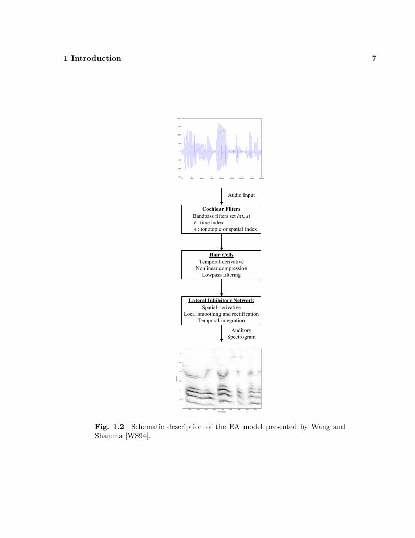
The EA model was developed based on investigations at various stages of the auditory
system. Fig. 1.2 shows the structure of the EA model presented in [WS94], wherein a dig-
itized input signal (e.g., 16-bit signed pulse-code modulation (PCM) data with a sampling
rate of 16 kHz) passes through the following three processing stages:
• Cochlear filters : A set of bandpass filters h(t, s) is used to describe the response
characteristics of the basilar membrane (BM), wherein t is the time index and s
denotes a specific location on the BM.
• Hair cells : The process at this stage can be modeled by a temporal derivative, a
sigmoid-like nonlinear compression, and a lowpass filtering. At this stage, the motion
on the BM is transformed into neural spikes in the auditory nerves.
• Lateral inhibitory network (LIN): The operations at this stage include a derivative
with respect to the tonotopic or spatial axis s, a local smoothing, a half-wave rec-
tification, and a temporal integration. Discontinuities along the cochlear axis s are
detected at this stage.
For a frame of input signal, these operations effectively compute a so-called auditory spec-
trum1.
Following the analysis in [WS94], the noise-robustness of the EA model can be at-
tributed in part to its self-normalization property which causes spectral enhancement or
noise suppression. To explore the nature of the self-normalization, Wang and Shamma
have conducted a qualitative analysis, followed by a quantitative analysis wherein a closed-
form expression of the auditory spectrum is derived [WS94]. For the quantitative analysis,
because of the nonlinear nature of the EA model, only a special simplified case has been
studied wherein a step function is used to replace the original nonlinear sigmoid compression
function at the second processing stage in Fig. 1.2.
The noise-robustness of the original EA model has been demonstrated in different ap-
plications such as audio classification [WS94, RA04]. However, this model is characterized
1As usual, auditory spectrogram refers to the three-dimensional plot of auditory spectra over time.
1 Introduction 7
Cochlear Filters
Bandpass filters set h(t, s)
t : time index
s : tonotopic or spatial index
Hair Cells
Temporal derivative
Nonlinear compression
Lowpass filtering
Lateral Inhibitory Network
Spatial derivative
Local smoothing and rectification
Temporal integration
Audio Input
Auditory
Spectrogram
Time (ms)
Channel
100 200 300 400 500 600 700 800 900
20
40
60
80
100
120
0 2000 4000 6000 8000 10000 12000 14000 16000-3000
-2000
-1000
0
1000
2000
3000
4000
Fig. 1.2 Schematic description of the EA model presented by Wang andShamma [WS94].
1 Introduction 8
by high computational requirements and nonlinear processing, which may prevent its use
in certain practical applications.
Motivated by the existing work on EA model [WS94], we seek in this thesis to further
explore its noise-suppression property from a broader perspective, and to develop simplified
implementations of this property for applications to a broad class of audio classification
tasks. Accordingly, the following sub-objectives are established in this work:
• With respect to the limitation of the quantitative analysis conducted in [WS94], it is
of interest to investigate the noise-suppression property from a broader perspective,
i.e., to derive a closed-form expression for auditory spectrum using a more general
sigmoid-like function, and to conduct relevant analysis.
• Considering the computational complexity of the original EA model, it is desirable
that the model be further simplified. Specifically, a frequency-domain approximated
realization with noise-suppression property implemented, wherein efficient FFT algo-
rithms are available, may be of significant practical interest.
• The noise-suppression property implemented in the proposed simplified realization
needs to be evaluated through audio classification experiments. Ideally, the clas-
sification performance of the audio features obtained from the proposed simplified
implementation should be compared to that of some conventional features such as
MFCCs.
• To further explore the proposed frequency-domain simplified implementation from a
practical perspective, it is desirable to implement an audio classification algorithm,
which involves the use of audio features obtained from the simplified implementation,
on a floating-point DSP platform.
1.3 Main Contributions
As indicated above, the main focus of this research is on the noise-suppression property
of the EA model [WS94], together with its application in audio classification. The main
contributions are summarized below.
1 Introduction 9
1.3.1 Extended Analysis of Self-Normalization
Having noticed the general nonlinear compression nature of the Gaussian cumulative distri-
bution function (CDF), and the resemblance between the graph of the sigmoid function and
that of the Gaussian CDF, we use the latter as an approximation to the original sigmoid
compression function to derive a new closed-form expression for the auditory spectrum at
the output of the EA model, and to conduct further relevant analysis. The new results
based on the Gaussian CDF verify the self-normalization property as analyzed in [WS94].
Compared to the original analysis wherein a step function is used to approximate the non-
linear sigmoid compression function, a Gaussian CDF provides a better, yet mathematically
tractable, approximation in the analysis.
1.3.2 Simplification/Approximation of the Auditory Spectrum
Based on the original time-domain analysis in [WS94], a simplified auditory spectrum is
proposed, which provides a way to investigate or approximate the EA model from a linear
perspective. The underlying analysis naturally leads itself to frequency-domain approaches
for approximation in order to achieve a significant reduction in the computational com-
plexity of the EA model.
Such a simplified FFT-based spectrum is then proposed wherein a local spectral self-
normalization is implemented through the use of a pair of wide and narrow filters defined in
the frequency domain. A simplified scheme is also proposed for power spectrum grouping
with emphasis on the low-frequency components. The classification performance of the
proposed FFT-based spectrum is comparable to that of the original auditory spectrum
while its computational complexity is much lower.
An improved implementation of the above FFT-based spectrum is further proposed to
calculate a so-called FFT-based auditory spectrum. The introduced improvements include
the use of characteristic frequency (CF) values of the cochlear filters in the original EA
model for power spectrum selection, and the use of a pair of fast and slow running averages
over the frequency axis to implement the spectral self-normalization. With the introduced
improvements, the proposed FFT-based auditory spectrum allows more flexibility in the
extraction of noise-robust audio features.
1 Introduction 10
1.3.3 Setup of the Audio Classification Experiment
To evaluate the performance of the proposed simplified FFT-based spectra2, some audio
classification experiments are designed and carried out. The main distinguishing features
of our experimental setup can be summarized as follows:
• Audio sample database: To carry out audio classification tests, two generic audio
databases are built which include speech, music, and noise clips. The sampling rates
of the two audio sample databases are 16 kHz and 8 kHz, whereas the total lengths
are 200 min and 140 min, respectively.
• Audio feature: Audio features are calculated over short (frame level) and long (clip
level) time periods. For the original auditory spectrum [WS94] and the two proposed
FFT-based simplified spectra, discrete cosine transform (DCT)-based features are
calculated. In addition, a set of spectral features are calculated using the proposed
FFT-based simplified auditory spectrum. The clip-level features used in this study
are simply the statistical mean and variance values of the corresponding frame-level
features.
• Classification test : Three-class (i.e., speech, music and noise) and two-class (noise
and non-noise) classification experiments have been conducted to evaluate the per-
formance. Specifically, mismatched tests are designed to evaluate the noise-robustness
of various features, wherein the training and testing sets contain samples with mis-
matched SNR values.
1.3.4 DSP Demo System
To further explore the proposed FFT-based auditory spectrum from a practical audio clas-
sification perspective, a floating-point DSP implementation is developed and tested. A
three-class audio classification algorithm using the DCT-based feature set and a C4.5 deci-
sion tree model [Qui93] is implemented on Texas Instruments TMS320C6713 DSP Starter
Kit (DSK) [Spe04, ?]. The input audio signals are 16-bit signed PCM data which are sam-
pled at 16 kHz and stored on the host PC. The outputs of the system are audio classification
2These include the proposed FFT-based spectrum and the proposed FFT-based auditory spectrum asdiscussed in Section 1.3.2
1 Introduction 11
decisions on a 1 s basis. Through the use of a pair of host channels, the connection between
the host PC and DSP target board has been established in the presented implementation.
A simple Matlab algorithm is also developed to monitor the real-time outputs from the
DSP target.
By using the available real-time software development tools [Tex05a], we have investi-
gated the computational complexity of the algorithm. Through the use of different opti-
mization approaches, including the tools and optimized functions provided by the C6713
DSK, a significant reduction in the computational complexity is achieved for the proposed
implementation.
1.3.5 Publications
The above contributions lead to a number of publications in peer-reviewed journals and
conference proceedings, listed as [CC08, CC06b, CC06c, CC06a, CC07] in the reference
section.
1.4 Thesis Organization
The proposed research work will be presented in detail in the next few chapters according
to the following outline:
In Chapter 2, a literature review is presented covering audio classification algorithms
presented in the recent decade from three perspectives, i.e., audio signals, audio features
and classification approaches.
The EA model presented by Wang and Shamma [WS94], the original analysis of the
self-normalization property, and the application of this model in audio classification, are
summarized in Chapter 3. Several open research problems are further presented which form
the basis of the proposed research on auditory-inspired noise-robust audio classification
algorithms.
As an extension to the original analysis in [WS94], the proposed analysis of self-
normalization using the Gaussian CDF approximation is presented in Chapter 4.
Chapter 5 details our efforts to develop simplified FFT-based spectra wherein the noise-
suppression property inherited from the original auditory spectrum are implemented.
The general setup of the classification experiment is presented in Chapter 6, wherein
the audio database, the extraction of different audio features, and the implementation
1 Introduction 12
of classification algorithms are detailed. The classification performance of different audio
features is compared and analyzed.
Chapter 7 describes the implementation of a demo system based on the C6713 DSK,
wherein the algorithm uses DCT-based features obtained from the proposed FFT-based
auditory spectrum. Different optimization approaches are applied to reduce the computa-
tional complexity of this system.
Chapter 8 concludes this thesis by summarizing the main contributions and discussing
possible future research avenues.
13
Chapter 2
A Review of Audio Classification
Algorithms
Content-based audio analysis has existed for some time. In certain applications, the main
focus is on the speech or text information, e.g., text retrieval, documentary indexing,
multi-speaker change detection [YBF+97, VBDT99, HH04]. For a multimedia document,
its semantic meanings are embedded in multiple forms, including audio and video data.
Therefore, a content-based analysis over all types of data would provide a more accurate
description. As an important part of multimedia documents, audio data can provide useful
information for content-based analysis. Indeed the past decade has seen extensive research
on audio-based content analysis, due to the relative simplicity of the processing procedures
and the effectiveness of the content analysis.
In this work, we focus on audio classification algorithms. In recent years, different
audio classification algorithms have been proposed along with excellent performance be-
ing reported. In this chapter, an overview is presented on audio classification algorithms
from the following three perspectives: audio signals, audio features, and classification ap-
proaches.
2 A Review of Audio Classification Algorithms 14
2.1 Audio Signals
2.1.1 Speech and Music Classification
As the two most popular audio classes in multimedia communications, speech and music
attract much attention in audio classification applications. In an early study by Saunders
[Sau96], a simple technique has been proposed to discriminate speech from music by only
using time-domain features such as the zero-crossing rate (ZCR) and energy. The minimal
computation associated with the proposed approach may lend itself to implementations in
radio receivers at very low add-on cost. A correct classification rate of 98% was reported. In
another work, to classify speech and music on FM radios, Scheirer and Slaney employed as
many as 13 features, such as the 4-Hz modulation energy, pulse metric, spectral centroid,
spectral rolloff point, etc. [SS97]. The speech samples used in this work include those
spoken by both male and female speakers. For music samples, the database includes jazz,
pop, country, salsa, reggae, classical, various non-Western styles, various sorts of rock, and
new age music, both with and without vocals. A correct classification rate of 94.2% has
been reported for 20 ms segments and 98.6% for 2.4 s segments. A similar work done by
Carey et al. has compared the discrimination performance achieved by different features,
such as the pitch, amplitude features, ZCR, etc., wherein the gaussian mixture model
(GMM) was used for classification [CPLT99]. In this work, the speech samples are spoken
in thirteen languages including Arabic, English, French, Mandarin, etc., whereas for the
music, besides a diverse selection of Western music, music clips from Eastern Asia, the
Arab world, Africa, South America and the Indian subcontinent are also included. Similar
research on speech/music classification can also be found in [AMB02, GL04, PT05].
Such speech/music classification sets can be used for listeners to surf radio channels
for segments of music or talk. It may also be used for long-term monitoring of a given
station for different purposes. A Low bit-rate audio coding algorithm is also an application
that can benefit from distinguishing speech from music. To design a universal coder that
can reproduce well both speech and music is a complex problem. An alternative approach
is to design a multi-mode coder that can accommodate different types of signals. The
appropriate module is selected using the output of a speech/music classifier. For example,
Qiao [Qia97] proposed an alternative approach to mixed speech/music coding. After music
signals are separated from speech, a G.722 coder and a G.723.1-based speech coder are used
for music and speech segments respectively. In [TRRL00], a speech/music discrimination
2 A Review of Audio Classification Algorithms 15
procedure for multi-mode wideband coding is described. An experimental CELP (code-
excited linear prediction)/transform coder operating at 16 kbit/s is demonstrated, wherein
an improved overall subjective quality is observed as compared to single-mode coders.
2.1.2 Environmental Sound and Background Noise
Besides speech and music, due to different considerations, some researchers have included
other audio classes in their studies, especially the environmental sound and background
noise, which are important elements in audio recordings.
In a content-based retrieval work by Wold et al. [WBKW96], the test sound database
contains about 400 sound files, varying in duration from less than one second to about 15
seconds. This database comprises a wide variety of sounds, including those from animals,
machines, musical instruments, speech, and nature.
Compared to some other studies, Zhang and Kuo have placed more emphasis on the
environmental sounds, an issue which was often ignored in the past [ZK99]. A hierarchical
system for audio classification and retrieval has been proposed, wherein audio clips are
first classified and segmented into speech, music, several types of environmental sounds
and silence; the environmental sounds are further classified into 10 sub-classes including
applause, birds’ cry, dog bark, explosion, foot step, laugh, rain, river flow, thunder, and
windstorm. The proposed work has achieved accuracy rates of 90% and 80% for the first
and second stages classification respectively.
Jiang et al. [JLZ00], Lu et al. [LZJ02], and Zhu and Zhou [ZZ03] each proposed an
audio or audio video combined classification/segmentation scheme, in which audio tracks
are classified into speech, music, environmental sound and silence. Sound effects that are
associated with highlight events in entertainments, sports, meetings and home videos, such
as laughter, applause, cheer, scream, etc., are considered in [CLZC03] and [ZBC03].
In practical applications, background sound and noise may be present together with
other audio signals like speech or music. These mixed or hybrid sounds have also been inves-
tigated in some research, for example, speech with background music [ZC01, LD04, NHK05],
speech with background noise (or noisy speech) [NHK05, WGY03, SA04], environmental
sound with background music [ZC01], and music presented in noisy conditions [SA04]. In
a work by Lu and Hankinson [LH00b], the level of the background sounds has been taken
into consideration wherein the audio database contains speech samples mixed with light
2 A Review of Audio Classification Algorithms 16
background noise/music, medium background noise, and heavy background noise/music.
Recently, Alexandre et al. proposed an automatic sound classifier for digital hearing
aids, which aims to enhance listening comprehension when the user goes from one sound en-
vironment to another [ACRLF07]. A two-layer classifying system is implemented, wherein
an audio signal is first classified into either speech or non-speech, and then the speech is
further classified into either speech in quiet (with no background noise or with a high SNR
ratio) or speech in presence of noise or music (vocal or nonvocal).
Indeed for modern hearing aids instruments, researchers have attempted to improve the
performance through the use of audio classification algorithms. In [Kat95], based on some
other studies, Kates concluded that different hearing aids characteristics are desirable under
different listening conditions. Accordingly, modern hearing aids normally provide several
hearing programs, each being designed for a specific listening environment (or acoustic sit-
uation), such as quiet environment or noisy environment. A set of common audio classes
from a hearing instrument point of view includes speech, music, stationary and nonstation-
ary noise [BB04]. A scheme for automatically adapting a hearing instrument for various
listening situations (e.g., speech, music, silence, noise, etc.) would free users from manually
switching. Nordqvist and Leijon [NL04] proposed an efficient and robust sound classifica-
tion algorithm which would enable a hearing aid to automatically change its behavior for
three listening environments, namely: speech in traffic noise, speech in babble, and clean
speech, regardless of the SNR value. A set of cepstral coefficient features is calculated
for the use of classification, and the estimated computational load is less than 0.1 million
instructions per second (MIPS) based on a Motorola 56k architecture [NL04].
In [RA05], Ravindran and Anderson presented a robust audio classification system that
could be used to switch automatically between different hearing aids algorithms based on
the auditory scene. A four-class audio classification task, i.e., speech, music, noise, and
speech in noise, is carried out to evaluate the performance of the proposed system. A
similar research is also found in [BALD05] wherein a sound classification system for the
automatic recognition of the acoustic environment in a hearing aid is proposed. Using
audio features that are inspired by auditory scene analysis, the system distinguishes four
sound classes, i.e., clean speech, speech in noise, noise, and music.
Some simple audio classification systems have been employed in the current hearing aids
instruments. Adapto, for example, is a product of Oticon, a successful Danish hearing aids
manufacturer and one of the world’s leading manufacturers of hearing aids products [Oti].
2 A Review of Audio Classification Algorithms 17
What has made Adapto unique are three revolutionary innovations, among which is the
VoiceFinder, an integrated sub-system that allows Adapto to accurately detect speech in
difficult listening situations. The VoiceFinder acts as a speech/noise classifier. It processes
incoming sound to provide maximum speech understanding. When no speech is present,
it automatically tunes out background noise and saves one from unnecessary annoyance.
A similar sound classification system, AutoSelect, is implemented in Phonak’s (based in
Stafa, Switzerland) Claro hearing systems, which can automatically switch between quiet
and noisy situations [Pho]. Once a switch has been activated, a different signal processing
strategy is applied to match a specific listening situation.
2.1.3 Use of Compressed Audio Data
Instead of the conventional waveform audio signal (i.e., PCM uncompressed data), some
algorithms have used compressed audio data directly. The use of compressed data is suitable
for large-size audio or video files, which are often stored in certain compressed formats.
Using compressed data may lead to savings on the calculations related to the complex
decoding process.
In [NLS+99], a fast and accurate audio classification method is described on the Mov-
ing Picture Experts Group (MPEG)-1 Layer 2 coded data domain. Silence segments are
detected first; and then, non-silence segments are further classified into music, speech, and
applause. Jarina et al. [JOMM02] proposed an approach to speech/music discrimination
based on rhythm (or beat) detection. The discriminator uses just three features (i.e., the
width of the widest peak, peak rates, and the rhythm metric) that are computed from the
data directly taken from MPEG-1 Layer 2 bitstreams. A classification rate of 97.7% is
reported.
Recent years have seen a widespread usage of MPEG-1 Audio Layer 3 (MP3) audio and
a more efficient successor, MPEG Advanced Audio Coding (AAC) audio, as well as the
proliferation of video content carrying MP3 or AAC audio. With the emerging MP3/AAC
audio contents, research has been conducted to classify audio data using MP3/AAC en-
coded bitstreams. Tzanetakis and Cook investigated the calculation of spectral features
(e.g., centroid, rolloff point) directly from MPEG-2 Layer 3 compressed data [TC00]. Ex-
perimental results show that the proposed classification algorithms are comparable to those
working directly with PCM uncompressed audio data. Kiranyaz et al. presented a novel
2 A Review of Audio Classification Algorithms 18
perceptual based fuzzy approach to the classification and segmentation of MP3 and AAC
audio [KQG04]. The input audio segments are classified into speech, music, fuzzy or si-
lence. Lie and Su [LS04] investigated the content-based retrieval of MP3 songs based on
the query by singing wherein perceptual features were calculated from MDCT (modified
discrete cosine transform) coefficients.
2.2 Audio Features
A key issue in the development of an audio classification algorithm is the design of audio
features that can be used to discriminate different audio classes. A good feature is expected
to have a large interclass difference while maintaining a small intraclass difference.
Audio features are commonly extracted in two levels, the short-term frame level and the
long-term clip level [WLH00]. The concept of audio frame comes from traditional speech
signal processing, where a frame usually covers a length of around 10 to 40 ms within which
the signal is assumed to be stationary. However, to reveal the semantic meanings of an
audio signal, an analysis over a longer interval is more appropriate. A signal with such
a long interval is called an audio clip, usually with a length ranging from one second to
several tens of seconds. Clip-level features usually describe how frame-level features change
over a time window. Depending on different applications, the length of an audio clip could
be fixed or not. Audio frames and clips may overlap in time with their predecessors. Some
common frame-level and clip-level features are introduced below.
2.2.1 Frame-Level Features
The frame-level features are calculated through time-domain analysis, Fourier transform
analysis, linear predictive coding (LPC) analysis, etc.
Short-Time Energy
The short-time energy is a simple yet reliable feature. It is defined as
En =1
N
N∑i=1
x2n[i] (2.1)
2 A Review of Audio Classification Algorithms 19
where En denotes the nth frame energy, N is the frame length, and xn[i] represents the
ith sample in the nth frame1. The short-term energy can be used to distinguish audible
sounds from silence gaps when the SNR is high, or voiced speech from unvoiced speech. The
change pattern of the short-term energy over time may reveal the rhythm or periodicity
information. Short-term energy also provides a basis for normalization of the signal.
Instead of the short-term energy as defined in (2.1), some studies use the root-mean-
square (RMS) value, i.e., the so-called volume, or approximately the loudness [WBKW96,
PT05]. Some other studies consider energy features in the frequency domain, using either
the total power or the subband power as features [Li00, LCTC05].
Short-Time Average Zero-Crossing Rate
The short-time average zero-crossing rate (ZCR) can be defined as
ZCRn =1
2
N∑i=2
|sgn (xn[i])− sgn (xn[i− 1])| (2.2)
where ZCRn denotes the nth frame ZCR and sgn(·) is the sign function. Since unvoiced
speech typically has much higher ZCR values than voiced speech, the ZCR can be used to
distinguish between voiced and unvoiced speech [O’S00].
In [EMKPK00], a new ZCR-based feature, the linear prediction zero-crossing ratio (LP-
ZCR), is defined as the ratio of the ZCR of the input to the ZCR of the output of the LP
analysis filter (i.e., the LP residual signal). According to this study, the LP-ZCR quantifies
the correlation structure of the input sound. For example, a highly correlated sound such
as voiced speech has a low LP-ZCR, while unvoiced speech has a value above 0.5. For a
white noise the LP-ZCR is ideally one.
Pitch/Fundamental Frequency
A harmonic sound consists of a series of major frequency components including the fun-
damental frequency and its integer multiples. Pitch, a perceptual term, is also used to
represent the fundamental frequency. The typical pitch frequency for a human being is
1In case a windowing operation is involved in the short-time analysis, xn[i], i = 1, 2, · · · , N , representthe corresponding samples weighted by a specific window function.
2 A Review of Audio Classification Algorithms 20
between 50-450 Hz, whereas for music the value can be much larger [WLH00]. To design a
robust and reliable pitch detector for an audio signal is still an open research problem.
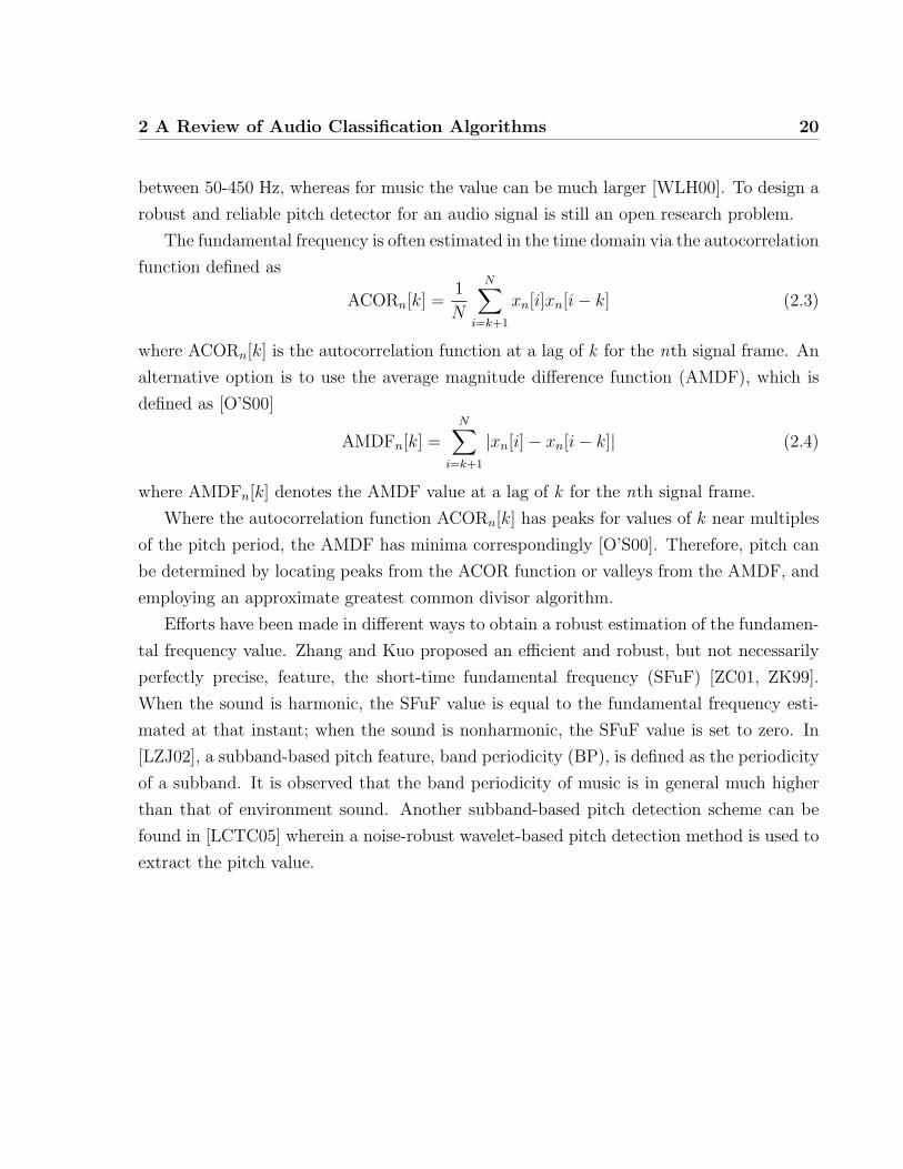
The fundamental frequency is often estimated in the time domain via the autocorrelation
function defined as
ACORn[k] =1
N
N∑i=k+1
xn[i]xn[i− k] (2.3)
where ACORn[k] is the autocorrelation function at a lag of k for the nth signal frame. An
alternative option is to use the average magnitude difference function (AMDF), which is
defined as [O’S00]
AMDFn[k] =N∑
i=k+1
|xn[i]− xn[i− k]| (2.4)
where AMDFn[k] denotes the AMDF value at a lag of k for the nth signal frame.
Where the autocorrelation function ACORn[k] has peaks for values of k near multiples
of the pitch period, the AMDF has minima correspondingly [O’S00]. Therefore, pitch can
be determined by locating peaks from the ACOR function or valleys from the AMDF, and
employing an approximate greatest common divisor algorithm.
Efforts have been made in different ways to obtain a robust estimation of the fundamen-
tal frequency value. Zhang and Kuo proposed an efficient and robust, but not necessarily
perfectly precise, feature, the short-time fundamental frequency (SFuF) [ZC01, ZK99].
When the sound is harmonic, the SFuF value is equal to the fundamental frequency esti-
mated at that instant; when the sound is nonharmonic, the SFuF value is set to zero. In
[LZJ02], a subband-based pitch feature, band periodicity (BP), is defined as the periodicity
of a subband. It is observed that the band periodicity of music is in general much higher
than that of environment sound. Another subband-based pitch detection scheme can be
found in [LCTC05] wherein a noise-robust wavelet-based pitch detection method is used to
extract the pitch value.
2 A Review of Audio Classification Algorithms 21
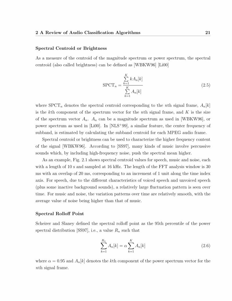
Spectral Centroid or Brightness
As a measure of the centroid of the magnitude spectrum or power spectrum, the spectral
centroid (also called brightness) can be defined as [WBKW96] [Li00]
SPCTn =
K∑k=1
kAn[k]
K∑k=1
An[k]
(2.5)
where SPCTn denotes the spectral centroid corresponding to the nth signal frame, An[k]
is the kth component of the spectrum vector for the nth signal frame, and K is the size
of the spectrum vector An. An can be a magnitude spectrum as used in [WBKW96], or
power spectrum as used in [Li00]. In [NLS+99], a similar feature, the center frequency of
subband, is estimated by calculating the subband centroid for each MPEG audio frame.
Spectral centroid or brightness can be used to characterize the higher frequency content
of the signal [WBKW96]. According to [SS97], many kinds of music involve percussive
sounds which, by including high-frequency noise, push the spectral mean higher.
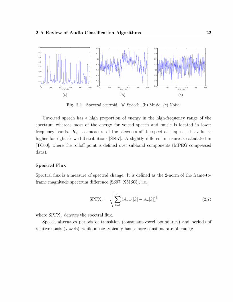
As an example, Fig. 2.1 shows spectral centroid values for speech, music and noise, each
with a length of 10 s and sampled at 16 kHz. The length of the FFT analysis window is 30
ms with an overlap of 20 ms, corresponding to an increment of 1 unit along the time index
axis. For speech, due to the different characteristics of voiced speech and unvoiced speech
(plus some inactive background sounds), a relatively large fluctuation pattern is seen over
time. For music and noise, the variation patterns over time are relatively smooth, with the
average value of noise being higher than that of music.
Spectral Rolloff Point
Scheirer and Slaney defined the spectral rolloff point as the 95th percentile of the power
spectral distribution [SS97], i.e., a value Rn such that
Rn∑k=1
An[k] = α
K∑k=1
An[k] (2.6)
where α = 0.95 and An[k] denotes the kth component of the power spectrum vector for the
nth signal frame.
2 A Review of Audio Classification Algorithms 22
0 200 400 600 800 10000
0.1
0.2
0.3
0.4
0.5
0.6
0.7
0.8
Time index
(a)
0 200 400 600 800 10000.1
0.12
0.14
0.16
0.18
0.2
0.22
0.24
Time index
(b)
0 200 400 600 800 10000.24
0.26
0.28
0.3
0.32
0.34
0.36
0.38
Time index
(c)
Fig. 2.1 Spectral centroid. (a) Speech. (b) Music. (c) Noise.
Unvoiced speech has a high proportion of energy in the high-frequency range of the
spectrum whereas most of the energy for voiced speech and music is located in lower
frequency bands. Rn is a measure of the skewness of the spectral shape as the value is
higher for right-skewed distributions [SS97]. A slightly different measure is calculated in
[TC00], where the rolloff point is defined over subband components (MPEG compressed
data).
Spectral Flux
Spectral flux is a measure of spectral change. It is defined as the 2-norm of the frame-to-
frame magnitude spectrum difference [SS97, XMS05], i.e.,
SPFXn =
√√√√ K∑k=1
(An+1[k]− An[k])2 (2.7)
where SPFXn denotes the spectral flux.
Speech alternates periods of transition (consonant-vowel boundaries) and periods of
relative stasis (vowels), while music typically has a more constant rate of change.
2 A Review of Audio Classification Algorithms 23
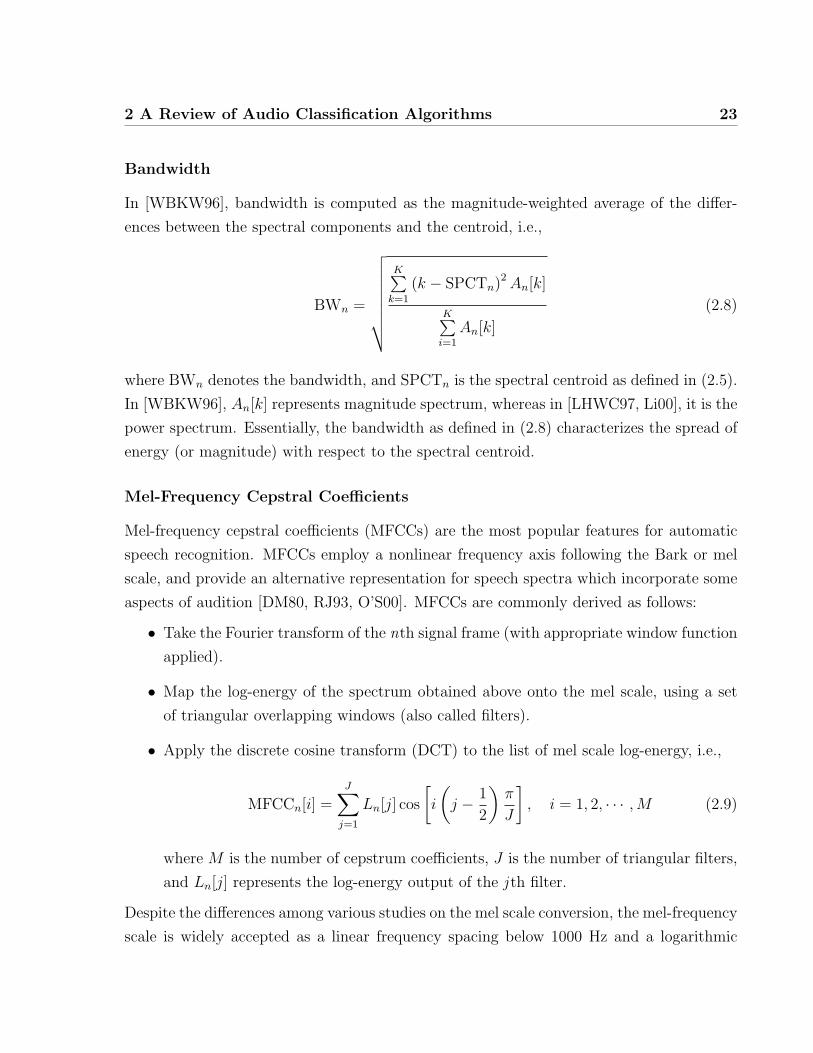
Bandwidth
In [WBKW96], bandwidth is computed as the magnitude-weighted average of the differ-
ences between the spectral components and the centroid, i.e.,
BWn =
√√√√√√√√K∑k=1
(k − SPCTn)2An[k]
K∑i=1
An[k]
(2.8)
where BWn denotes the bandwidth, and SPCTn is the spectral centroid as defined in (2.5).
In [WBKW96], An[k] represents magnitude spectrum, whereas in [LHWC97, Li00], it is the
power spectrum. Essentially, the bandwidth as defined in (2.8) characterizes the spread of
energy (or magnitude) with respect to the spectral centroid.
Mel-Frequency Cepstral Coefficients
Mel-frequency cepstral coefficients (MFCCs) are the most popular features for automatic
speech recognition. MFCCs employ a nonlinear frequency axis following the Bark or mel
scale, and provide an alternative representation for speech spectra which incorporate some
aspects of audition [DM80, RJ93, O’S00]. MFCCs are commonly derived as follows:
• Take the Fourier transform of the nth signal frame (with appropriate window function
applied).
• Map the log-energy of the spectrum obtained above onto the mel scale, using a set
of triangular overlapping windows (also called filters).
• Apply the discrete cosine transform (DCT) to the list of mel scale log-energy, i.e.,
MFCCn[i] =J∑j=1
Ln[j] cos
[i
(j − 1
2
)π
J
], i = 1, 2, · · · ,M (2.9)
where M is the number of cepstrum coefficients, J is the number of triangular filters,
and Ln[j] represents the log-energy output of the j th filter.
Despite the differences among various studies on the mel scale conversion, the mel-frequency
scale is widely accepted as a linear frequency spacing below 1000 Hz and a logarithmic
2 A Review of Audio Classification Algorithms 24
spacing above 1000 Hz [DM80]. Such a frequency spacing scale has been used to capture
the phonetically important characteristics of speech. In [DM80], a set of 20 triangular
windows was used wherein the frequency range covers up to around 5 kHz.
MFCCs are also found useful in audio classification applications [Li00]. Two properties
of MFCCs, one being that the first coefficient is proportional to the audio energy and the
other being that there is no correlation among different coefficients, make MFCCs attractive
in audio classification [LH00a].
In [KMS04], speaker recognition experiments have been conducted to evaluate the effi-
ciency of an audio indexing and retrieval system based on audio spectrum basis (ASB) and
audio spectrum projection (ASP) of MPEG-7 audio descriptors. The experimental results
indicate that MFCC features together with delta and double-delta MFCCs outperform
MPEG-7 features.
LPC-Related Features
A popular alternative to the short-time Fourier transform for speech signals is linear pre-
dictive coding (LPC) analysis [RS78, O’S00]. LPC estimates each speech sample based on
a linear combination of its previous samples. By minimizing the error between the actual
and the predicted samples over a finite interval, a set of predictor coefficients can be de-
termined, which provides an analysis-synthesis system for speech. The linear prediction is
closely related to the speech generation model wherein speech can be modeled as the out-
put of a linear, time-varying system excited by either quasi-periodic pulses (during voiced
speech), or random noise (during unvoiced speech) [RS78].
LPC is one of the most common techniques for low-bit-rate speech coding. The pop-
ularity of LPC comes from the relatively simple computation procedure yet precise repre-
sentation of the speech magnitude spectrum. LPC can be used to estimate basic speech
parameters, e.g., pitch, formants, vocal tract area function.
LPC analysis is also employed in audio classification to extract frame-level features. El-
Maleh et al. [EMKPK00] proposed a frame-by-frame classification scheme based on 10th
order line spectrum frequency (LSF) (also called line spectrum pair (LSP)) coefficients and
the differential LSFs. The LSF-based features are extracted to capture the fine spectral
variations between speech and music. According to [EMKPK00], small differential LSPs
indicate that the energy peaks are tightly packed while larger values can be interpreted as
2 A Review of Audio Classification Algorithms 25
a broader distribution. A similar analysis can be found in [JLZ00] wherein LSF analysis is
employed to refine the classification results from a pre-classifier.
In [XMS05], the so-called linear prediction coefficients-derived cepstrum coefficients
(LPCCs) are employed. Test results show that LPCCs are much better than LP coefficients
in identifying vocal music. Besides, according to [XMS05], the performance of the LP
coefficients and LPCCs can be improved by 20%-25% if the LP coefficients or LPCCs are
calculated in subbands.
2.2.2 Clip-Level Features
Some clip-level features are designed to characterize the temporal variation of frame-level
features (i.e., they are calculated using frame-level features), whereas others are designed
without the use of frame-level features. The most widely used clip-level features are the
statistical mean and variance values of frame-level features such as the energy and ZCR.
In addition, there are many other clip-level features as introduced below.
Energy-Based Features
The percentage of low energy frames is proposed in [SS97] to represent the variation of the
short-time energy. It is defined as the proportion of frames with RMS (root mean square)
power less than 50% of the mean RMS power within a window of 1 s. A similar feature,
low short-time energy ratio (LSTER), is defined in [LZJ02] and [JLZ00] as
LSTER =1
2Nf
Nf−1∑n=0
[sgn(0.5 E − En) + 1
](2.10)
where Nf is the number of frames in a clip, En represents the nth frame energy, E denotes
the average short-time energy in a window of 1 s, and sgn(·) is the sign function. In general
there are more silence frames in speech than in music. As a result, the LSTER measure of
speech will be much higher than that of music. According to [LZJ02], when using LSTER
as the only feature to discriminate speech from music, the error rate is 8.27%.
Normalized RMS variance is defined in [PT05] as the ratio of the RMS variance to the
square of the RMS mean, wherein here RMS value corresponds to the square-root value of
the frame energy. The generalized χ2 distribution is used to approximate the distribution
2 A Review of Audio Classification Algorithms 26
of RMS values. With a separation threshold of 0.24, 88% of the speech segments and 84%
of the music segments can be correctly identified [PT05].
Energy features are also considered in the subband domain, for example, in [NLS+99].
In [SS97], a so-called 4-Hz modulation energy is proposed where the calculation is based
on the energy distribution in 40 perceptual subbands. This feature is based on a generally-
accepted observation that speech has a characteristic energy modulation peak around the
4 Hz syllabic rate. Speech tends to have more modulation energy at 4 Hz than music does.
ZCR-Based Features
Speech signals produce a marked rise in ZCR during periods of unvoiced speech (especially
fricatives). As a result, the distribution of ZCR for speech signals is skewed towards the
high end, generating a distribution different from music signals, whose ZCR variation is not
distributed with the same bimodality as voiced and unvoiced speech [Sau96]. To capture
the lopisideness of the distribution of ZCR, Saunders [Sau96] employed a set of features
including the standard deviation of the first order difference of the ZCR, the third central
moment about the mean, the total number of zero crossings exceeding a threshold, and the
difference between the number of zero crossing samples above and below the mean.
A so-called high zero-crossing rate ratio (HZCRR) is designed in [JLZ00] and [LZJ02]
to reflect the skewness of the ZCR distribution. It is defined as follows [LZJ02]:
HZCRR =1
2Nf
Nf−1∑n=0
[sgn(ZCRn−1.5 ZCR) + 1
](2.11)
where ZCRn is the nth frame ZCR, and ZCR is the average ZCR in a 1 s window. According
to [LZJ02], if HZCRR alone is used to discriminate speech from music, the error rate is
19.36%.
Since there are always some silence intervals in a speech, the occurrence of null zero-
crossings (i.e., ZCR = 0) can be used to identify speech. Based on this, the ratio of null
zero-crossings can be used to identify speech segments [PT05]. However, the accuracy of
this feature may be affected by the presence of background noise or a change of speaking
rate.
2 A Review of Audio Classification Algorithms 27
Spectrogram-Based Features
An FFT-based or other sort of spectrogram effectively describes the spectral-temporal pat-
tern of an audio clip. In [ZC01], a feature called spectral peak track is determined by detect-
ing peaks in the power spectrum generated by the autoregressive (AR) model parameters
and checking harmonic relations among the peaks. For sounds from musical instruments,
their spectral peak tracks usually last for a certain period of time while remaining at the
same frequency level. Sounds from human voices have harmonic peak tracks which align
tidily in the shape of a comb. For songs, there are relatively long and stable tracks because
the voice may stay at a certain note for a period of time. Meanwhile, due to the vibration
of vocal cords, the spectral peak tracks in songs are often in a ripple-like shape. However,
for speech segments, the spectral peak tracks normally lie in lower frequency bands, and
tend to be shorter because there are intermissions between voiced syllables. In addition, the
spectral peaks may fluctuate slowly because the pitch may change during the pronunciation
of certain syllables.
In [LZJ02], an average spectral flux is proposed. It is defined as the average variation
value of spectra between two adjacent frames in a one-second window. It is found that in
general this value for speech is higher than that of music. In addition, the average spectral
flux for environment sound is among the highest and it changes more dramatically than
speech or music.
Rhythm and Tempo
In [SS97], a novel feature, called pulse metric, is calculated to determine the amount of
“rhythmicness” in a window of 5 s. The presented approach divides the signal into six
bands and finds the peaks using autocorrelations in the envelopes of each band, where the
peaks correspond roughly to perceptual onsets. According to [SS97], pulse metric may
indicate whether there is a strong, driving beat (i.e., techno, salsa) in the signal. Instead
of the autocorrelation method as presented in [SS97], Scheirer proposed another method
wherein banks of parallel comb filters are used to analyze the tempo of, and extract the
beat from, musical signals [Sch98].
A similar feature is proposed in [JOMM02] to classify speech and music wherein rhyth-
mic pulses are detected using a long-term autocorrelation method and with MPEG-1 en-
coded bitstreams.
2 A Review of Audio Classification Algorithms 28
In [FU01], a feature called beat spectrum is proposed to characterize the rhythm and
tempo of music and audio. The beat spectrum is a measure of acoustic self-similarity as
a function of time lag. A distance measure is used to calculate the similarity between
all pairwise combinations of feature vectors. The beat spectrogram is also proposed to
graphically illustrate rhythm variation over time.
Others
There are many other clip-level features. For example, a noise frame ratio (NFR) is pro-
posed in [LZJ02], where it is defined as the ratio of the number of noise frames to the
number of total frames in a given audio clip. Also in [LZJ02], the LSP dissimilarity be-
tween two one-second audio clips is measured to discriminate speech and noisy speech from
music.
In [PRAO03], based on observations of signals and spectrograms suggesting that music
appears to be more “ordered” than speech, entropy modulation is proposed to measure the
“disorder” of speech and music. Using the entropy computed from each signal frame (16
ms), the entropy modulation is calculated over a 1 s window. Entropy modulation is higher
for speech than for music [PRAO03].
2.3 Classification Methods
Depending on different requirements, the classifiers employed in audio classification range
from simple rule-based methods to more complex pattern recognition approaches. The
rule-based classifiers, such as those used in [ZC01, PT05, JOMM02], are often used in an
application where there is a requirement for real-time processing. Other pattern recognition
approaches commonly used in audio classification applications include the hidden Markov
model (HMM), the support vector machine (SVM), the Gaussian mixture model (GMM),
etc. A brief introduction to these classification approaches is given below.
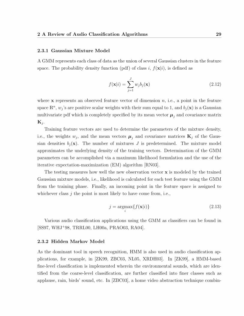
2 A Review of Audio Classification Algorithms 29
2.3.1 Gaussian Mixture Model
A GMM represents each class of data as the union of several Gaussian clusters in the feature
space. The probability density function (pdf) of class i, f(x|i), is defined as
f(x|i) =J∑j=1
wjbj(x) (2.12)
where x represents an observed feature vector of dimension n, i.e., a point in the feature
space Rn, wj’s are positive scalar weights with their sum equal to 1, and bj(x) is a Gaussian
multivariate pdf which is completely specified by its mean vector µj and covariance matrix
Kj.
Training feature vectors are used to determine the parameters of the mixture density,
i.e., the weights wj, and the mean vectors µj and covariance matrices Kj of the Gaus-
sian densities bj(x). The number of mixtures J is predetermined. The mixture model
approximates the underlying density of the training vectors. Determination of the GMM
parameters can be accomplished via a maximum likelihood formulation and the use of the
iterative expectation-maximization (EM) algorithm [RN03].
The testing measures how well the new observation vector x is modeled by the trained
Gaussian mixture models, i.e., likelihood is calculated for each test feature using the GMM
from the training phase. Finally, an incoming point in the feature space is assigned to
whichever class j the point is most likely to have come from, i.e.,
j = argmaxi{f(x|i)} (2.13)
Various audio classification applications using the GMM as classifiers can be found in
[SS97, WHJ+98, TRRL00, LH00a, PRAO03, RA04].
2.3.2 Hidden Markov Model
As the dominant tool in speech recognition, HMM is also used in audio classification ap-
plications, for example, in [ZK99, ZBC03, NL05, XRDH03]. In [ZK99], a HMM-based
fine-level classification is implemented wherein the environmental sounds, which are iden-
tified from the coarse-level classification, are further classified into finer classes such as
applause, rain, birds’ sound, etc. In [ZBC03], a home video abstraction technique combin-
2 A Review of Audio Classification Algorithms 30
ing audio and video features is presented, wherein the background sound, which is obtained
from the first-stage classification, is further classified into laughter, applause, scream and
others using HMM.
As a generative modeling approach, HMM describes a stochastic process with hidden
variables that produces the observable data. For the speech recognition problem, the
underlying assumption of the HMM is that the speech signal can be well modeled as a
parametric random process, and the corresponding parameters can be estimated in a well-
defined manner [Rab89, RJ93].
Taking Zhang and Kuo’s work as an example [ZK99], a hidden Markov model with
continuous observation densities and explicit state duration densities is used to model each
class of sound. The complete parameter set of the HMM is represented as
λ = (A,B,D,π) (2.14)
where A is the transition probability matrix, B denotes the parameters of the observation
density, D denotes the parameters of the duration density, and π represents the initial state
distribution. To train the HMM parameters, the parameters of the observation density,
which take the form of Gaussian mixtures, are first estimated for each state through a
maximum likelihood iteration process. Then, the transition probability and the duration
density parameters are calculated statistically according to the state indices of feature
vectors in the training set. The initial state distribution is usually set as
πi =1
N, 1 ≤ i ≤ N (2.15)
where N is the number of states.
In [ZK99], HMM parameter sets are built for ten different classes of sounds, which
include applause, birds’ cry, dog bark, explosion, foot step, laugh, rain, river flow, thunder,
and windstorm. That is, there are ten classes of sounds modeled with parameter sets
λi, 1 ≤ i ≤ 10. Feature vectors X = {x1,x2, · · · ,xT} are extracted from 6 to 8 sound
clips, and used for building the model for each audio class. The features used are taken
directly from the coefficients of a 128-point FFT applied to the audio signal, i.e., a feature
vector of 65 dimensions corresponding to the logarithm of the amplitude spectrum between
normalized frequency 0 and π. Information about timbre and rhythm is embedded in the
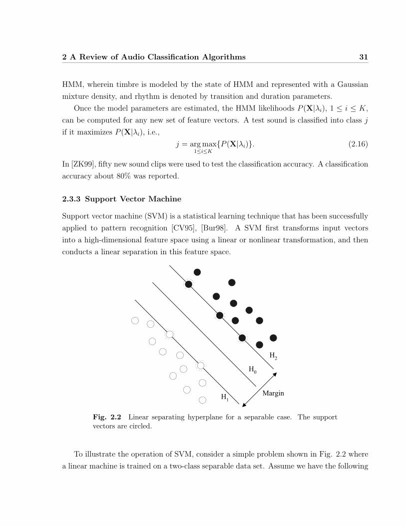
2 A Review of Audio Classification Algorithms 31
HMM, wherein timbre is modeled by the state of HMM and represented with a Gaussian
mixture density, and rhythm is denoted by transition and duration parameters.
Once the model parameters are estimated, the HMM likelihoods P (X|λi), 1 ≤ i ≤ K,
can be computed for any new set of feature vectors. A test sound is classified into class j
if it maximizes P (X|λi), i.e.,
j = arg max1≤i≤K
{P (X|λi)}. (2.16)
In [ZK99], fifty new sound clips were used to test the classification accuracy. A classification
accuracy about 80% was reported.
2.3.3 Support Vector Machine
Support vector machine (SVM) is a statistical learning technique that has been successfully
applied to pattern recognition [CV95], [Bur98]. A SVM first transforms input vectors
into a high-dimensional feature space using a linear or nonlinear transformation, and then
conducts a linear separation in this feature space.
H1
H2H0
Margin
Fig. 2.2 Linear separating hyperplane for a separable case. The supportvectors are circled.
To illustrate the operation of SVM, consider a simple problem shown in Fig. 2.2 where
a linear machine is trained on a two-class separable data set. Assume we have the following
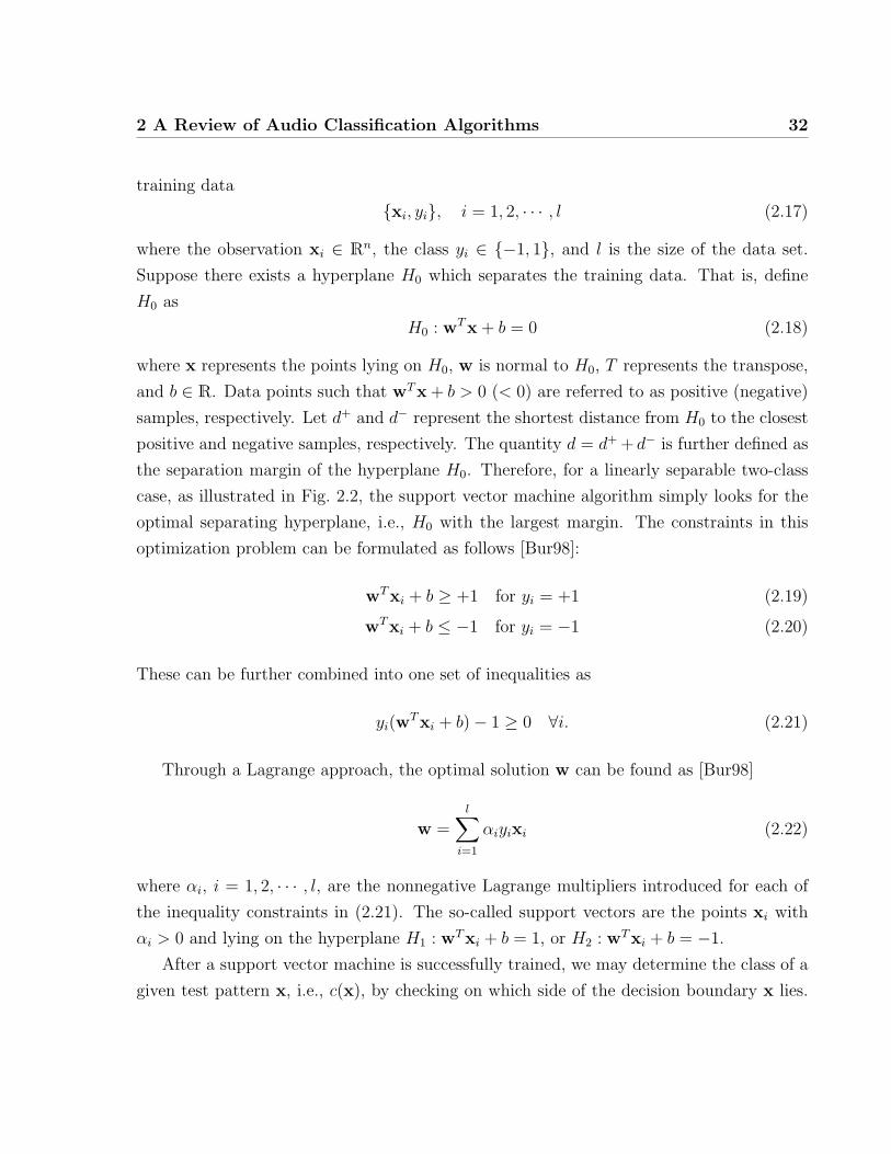
2 A Review of Audio Classification Algorithms 32
training data
{xi, yi}, i = 1, 2, · · · , l (2.17)
where the observation xi ∈ Rn, the class yi ∈ {−1, 1}, and l is the size of the data set.
Suppose there exists a hyperplane H0 which separates the training data. That is, define
H0 as
H0 : wTx + b = 0 (2.18)
where x represents the points lying on H0, w is normal to H0, T represents the transpose,
and b ∈ R. Data points such that wTx + b > 0 (< 0) are referred to as positive (negative)
samples, respectively. Let d+ and d− represent the shortest distance from H0 to the closest
positive and negative samples, respectively. The quantity d = d+ + d− is further defined as
the separation margin of the hyperplane H0. Therefore, for a linearly separable two-class
case, as illustrated in Fig. 2.2, the support vector machine algorithm simply looks for the
optimal separating hyperplane, i.e., H0 with the largest margin. The constraints in this
optimization problem can be formulated as follows [Bur98]:
wTxi + b ≥ +1 for yi = +1 (2.19)
wTxi + b ≤ −1 for yi = −1 (2.20)
These can be further combined into one set of inequalities as
yi(wTxi + b)− 1 ≥ 0 ∀i. (2.21)
Through a Lagrange approach, the optimal solution w can be found as [Bur98]
w =l∑
i=1
αiyixi (2.22)
where αi, i = 1, 2, · · · , l, are the nonnegative Lagrange multipliers introduced for each of
the inequality constraints in (2.21). The so-called support vectors are the points xi with
αi > 0 and lying on the hyperplane H1 : wTxi + b = 1, or H2 : wTxi + b = −1.
After a support vector machine is successfully trained, we may determine the class of a
given test pattern x, i.e., c(x), by checking on which side of the decision boundary x lies.
2 A Review of Audio Classification Algorithms 33
That is,
c(x) = sgn(wTx + b) = sgn
(l∑
i=1
αiyixTi x + b
)(2.23)
where sgn(·) is the sign function.
In cases the data are not linearly separable, but nonlinearly separable, a nonlinear
support vector classifier can be constructed using a kernel function K(xi,x) to replace
the product xTi x that characterizes the linear case [CV95, Bur98]. For example, we now
determine the class of a given test pattern x as
c(x) = sgn
(l∑
i=1
αiyiK(xi,x) + b
)(2.24)
where the model parameters αi and b are obtained through training. Commonly used
kernel functions include the polynomial function, the Gaussian radial basis function, and
the sigmoid function.
Although the SVM classifiers described above are binary in nature, they can be com-
bined to handle multiclass cases. A simple way is to take a “one-versus-rest” strategy to
train N classifiers, and determine the class for a test point which corresponds to the largest
distance [Bur98]. There are more efficient SVM algorithms proposed to handle multiclass
classification problems, e.g., in [CS01, TJHA05].
It is found in some studies that SVM is much more effective than other conventional
classifiers in terms of the classification accuracy, computation time, and stability to the
parameter settings [LCTC05]. For example, in [Sch00], SVM is shown to outperform neural
networks and k -nearest neighbor classifiers in a handwritten digits recognition task.
Recent years have seen increasing interest in the use of SVM in audio classification
applications [MR00, ZBC03, GL03, LD04, MSS04, XMS05, LCTC05]. For example, in
[LD04], four binary SVM classifiers are trained for a multiclass classification among seven
audio classes. Test results show that the proposed SVM-based method outperforms the
decision tree-based and the threshold-based audio classification schemes.
2.3.4 Nearest Neighbor
The nearest neighbor algorithm is relatively simple to implement. The main work of the
training phase is to store feature vectors and the corresponding class labels of the training
2 A Review of Audio Classification Algorithms 34
samples. To classify a new observation point x, the nearest neighbor algorithm examines
the local neighborhood of this point in the feature space and determines which training
point is closest to it. Observation x is then classified into the category of its nearest
neighbor.
If the number of the training points is large, instead of the single nearest neighbor, it is
more appropriate to consider K nearest neighbors. This leads to the K-nearest-neighbor
(KNN) algorithm, wherein a majority vote is conducted among the nearest K neighbors
and the test point is assigned to the class that is most common among its K nearest
neighbors [Fuk90]. The neighbors are taken from a set of training data. Euclidean distance
is commonly used for the KNN algorithm.
In [WBKW96], a nearest neighbor classifier based on a weighted Euclidean distance
measure is employed. One major disadvantage of the nearest-neighbor classifier is the need
to store a large number of training vectors, resulting in a large amount of computations
[EMKPK00]. In [SS97], a so-called k-d spatial classification algorithm is presented to ap-
proximate the KNN approach by voting only among those training points in the particular
region of the feature space grouped together by the k-d tree partitioning. This approximate
algorithm is proved to be faster than the conventional KNN classifier in a speech/music
classification application in [SS97].
2.3.5 Neural Network
An artificial neural network (ANN), or simply a neural network, grew out of research in
artificial intelligence (AI). An ANN attempts to mimic the fault-tolerance and capacity to
learn of the human brain by modeling its low-level structure. ANN refers to a mathematical
or computational model, consisting of a set of interconnected artificial neurons that are
characterized by a set of input values, the associated weights, and a function that sums
the weights and maps the result to an output [RN03]. An ANN processes training data
one at a time, and “learns” by comparing the output class with the known actual class of
the training data. The errors from the initial classification of the first data are fed back
into the network to modify the networks’ parameters, and so on for many iterations until
certain training criteria are achieved.
The feedforward, back-propagation architecture is the most popular, effective, and easy-
to-learn model for complex, multi-layered networks. The typical back-propagation network
2 A Review of Audio Classification Algorithms 35
has an input layer, an output layer, and at least one hidden layer. The number of layers and
the number of processing elements per layer are important parameters in the design of an
ANN. Unfortunately, there is no clear answer to the optimal choice of these parameters for
a particular application. It is the “art” of the network designer. In applications, scientists
usually follow some general rules, which are developed over time, to set these parameters;
to some extent, this represents the art of the ANN design.
Over the years, ANN has emerged as a promising alternative to various conventional
classification methods due to several advantages including the nonlinear modeling ability,
which makes them flexible in modeling real world complex relationships [Zha00]. For ex-
ample, a multiscale framework for five-class audio classification is proposed in [ZZ04]. Test
results indicate that the proposed neural network classifier outperforms other classifiers like
KNN. In [RSA05], compared to a GMM-based classifier, a neural network classifier with
features derived from an auditory model performs better in a four-class audio classification
task.
2.3.6 Linear Discriminant Analysis
Linear discriminant analysis (LDA) tries to find a linear combination of the extracted fea-
tures that best separates the group of cases [EKR04]. To represent the required linear
combination, a discrimination function is formed using the extracted features as discrim-
ination variables. After determining the first function that separates the groups as much
as possible, refined functions that improve the separation and are uncorrelated to previous
ones are further determined.
In [EKR04], using time-frequency analysis along with LDA, music clips are classified into
six different classes consisting of rock, classical, country, folk, jazz and pop. A similar work
can be found in [UKJ05]. Goodwin et al. proposed a LDA-based dynamic programming
segmentation algorithm for speech/music discrimination [GL04].
2.3.7 Other Classification Approaches
Many other pattern classification approaches have been applied in audio classification al-
gorithms besides the above introduced classifiers. For example, the AdaBoost algorithm
[RA05], [GZL01], the nearest feature line (NFL) approach [Li00], the maximum entropy
model based classifier [FZWL03], etc. In the development of an algorithm, the choice of a
2 A Review of Audio Classification Algorithms 36
specific classification method is determined by various factors, such as the requirements on
the computational complexity (including processing delay and memory requirement) and
the audio features employed in the algorithm.
2.4 Conclusion
In this chapter, a literature review has been presented on audio classification algorithms
from three perspectives, namely: audio signals, audio features, and classification approaches.
Regarding our proposed work, both three-class (i.e., speech, music and noise) and two-
class (i.e., noise and non-noise) classification experiments are conducted. The audio features
used in our experiments include conventional features such as MFCCs, features obtained
from the original auditory spectrum [WS94], and features obtained from the proposed
auditory-inspired FFT-based spectra. As for the classification approach, we use a SVM
algorithm and a decision tree learning algorithm. As introduced before, there has been
an increasing interest in the use of SVM in audio classification applications, and excellent
performance with SVM has been reported. In this work, we use the SVMstruct algorithm,
which is developed for predicting multivariate or structured outputs [TJHA05]. C4.5,
a widely used decision tree learning algorithm, is also used in our experiments for the
purpose of performance comparison [Qui93]. We will have more on these two classification
algorithms later in Chapter 6.
2 A Review of Audio Classification Algorithms 37
38
Chapter 3
Early Auditory Model and the
Noise-Suppression Property
As seen from the literature review presented in the previous chapter, some studies have
considered the presence of background noise in audio classification applications, for ex-
ample, in [LH00b, WGY03, SA04, NHK05, ACRLF07]. However, such considerations are
limited to using background noise as one of the audio classes or as a component of some
hybrid sounds. The effect of background noise on the performance of classification has not
been investigated widely. In fact, a classification algorithm trained using clean sequences
may fail to work properly when the actual testing sequences contain background noise with
certain SNR levels [RA04, MSS04].
The so-called early auditory (EA) model presented by Wang and Shamma [WS94] was
proved to be robust in noisy environments due to an inherent self-normalization property
that causes spectral enhancement or noise suppression. Recently, this model has been
employed in audio classification and noise-robust performance has been reported in [RA04].
Below, a brief introduction to the EA model [WS94] is presented, with emphasis on
its computational structure, its inherent self-normalization property, and an existing audio
classification task using this EA model. Based on the existing research on the EA model
and its application in audio classification, we further propose several research topics which
are either new or have only raised limited attention at this stage. These research topics
form the basis of our proposed study on auditory-inspired noise-robust audio classification
algorithms.
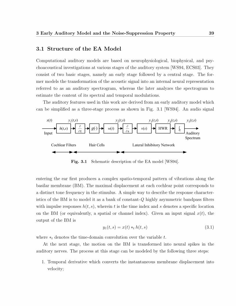
3 Early Auditory Model and the Noise-Suppression Property 39
3.1 Structure of the EA Model
Computational auditory models are based on neurophysiological, biophysical, and psy-
choacoustical investigations at various stages of the auditory system [WS94, ECS03]. They
consist of two basic stages, namely an early stage followed by a central stage. The for-
mer models the transformation of the acoustic signal into an internal neural representation
referred to as an auditory spectrogram, whereas the later analyzes the spectrogram to
estimate the content of its spectral and temporal modulations.
The auditory features used in this work are derived from an early auditory model which
can be simplified as a three-stage process as shown in Fig. 3.1 [WS94]. An audio signal
h(t,s) w(t) HWRv(s) ∫T
Lateral Inhibitory NetworkHair CellsCochlear Filters
Input AuditorySpectrum
y4(t,s)y1(t,s) y2(t,s) y3(t,s)
)(⋅g
y5(t,s)x(t)
t∂∂
s∂∂
Fig. 3.1 Schematic description of the EA model [WS94].
entering the ear first produces a complex spatio-temporal pattern of vibrations along the
basilar membrane (BM). The maximal displacement at each cochlear point corresponds to
a distinct tone frequency in the stimulus. A simple way to describe the response character-
istics of the BM is to model it as a bank of constant-Q highly asymmetric bandpass filters
with impulse responses h(t, s), wherein t is the time index and s denotes a specific location
on the BM (or equivalently, a spatial or channel index). Given an input signal x(t), the
output of the BM is
y1(t, s) = x(t) ∗t h(t, s) (3.1)
where ∗t denotes the time-domain convolution over the variable t.
At the next stage, the motion on the BM is transformed into neural spikes in the
auditory nerves. The process at this stage can be modeled by the following three steps:
1. Temporal derivative which converts the instantaneous membrane displacement into
velocity;
3 Early Auditory Model and the Noise-Suppression Property 40
2. Application of a sigmoid-like compression function g(·), which models the nonlinear
channel through the hair cells; and
3. Lowpass filtering w(t) which models the leakage of the cell membranes.
Therefore, the response of this stage can be described as
y2(t, s) = g
(∂
∂ty1(t, s)
)∗t w(t). (3.2)
At the last stage, a lateral inhibitory network (LIN) detects discontinuities along the
cochlear axis s. The operations can be divided into the following four steps:
1. Derivative with respect to s (i.e., along the tonotopic axis) which describes the lateral
interaction among LIN neurons;
2. Local smoothing with v(s), which accounts for the finite spatial extent of the lateral
interactions;
3. Half-wave rectification (HWR) which models the nonlinearity of the LIN neurons;
and
4. Temporal integration which reflects the fact that the central auditory neurons are
unable to follow rapid temporal modulations.
The operations at this stage can be summarized as follows [WS94]:
y3(t, s) =
(∂
∂sy2(t, s)
)∗s v(s)
=
{[g′(∂
∂ty1(t, s)
)∂2
∂s∂ty1(t, s)
]∗t w(t)
}∗s v(s) (3.3)
y4(t, s) = max(y3(t, s), 0) (3.4)
y5(t, s) = y4(t, s) ∗t Π(t) (3.5)
where Π(t) is a temporal integration function and ∗s denotes convolution along the tono-
topic, or the cochlear axis, s.
For a frame of input signal, these operations effectively compute a so-called auditory
spectrum. In practice, these operations can be implemented in the discrete-time domain
by use of appropriate digital filters.
3 Early Auditory Model and the Noise-Suppression Property 41
3.2 Noise-Suppression Property
In [WS94], through a stochastic analysis, this EA model was proved to be noise-robust due
to an inherent self-normalization property. The main results of this analysis are summarized
below.
3.2.1 Qualitative Analysis
Suppose the input signal x(t) can be modeled as a random process with zero mean. If
the bandwidth of the lowpass filter Π(t) is narrow enough, the output auditory spectrum,
y5(t, s), can be approximated by E[y4(t, s)] [WS94], where E[·] denotes statistical expecta-
tion. E[y4(t, s)] is referred to as an auditory spectrum in [WS94].
For the sake of simplicity, the temporal and spatial smoothing filters w(t) and v(s) are
ignored in the analysis [WS94]. From (3.4), we have [WS94]
E[y4(t, s)] = E
[max
(g′(∂
∂ty1(t, s)
)∂2
∂s∂ty1(t, s), 0
)]. (3.6)
Define quantities U and V as1 [WS94]
U ≡ U(t, s) =∂
∂ty1(t, s) =
(∂
∂tx(t)
)∗t h(t, s) (3.7)
V ≡ V (t, s) =∂2
∂s∂ty1(t, s) =
(∂
∂tx(t)
)∗t(∂
∂sh(t, s)
). (3.8)
Therefore, (3.6) can be rewritten as [WS94]
E[y4(t, s)] =
∫ ∞−∞
∫ ∞−∞
max(g′(u)v, 0)fUV (u, v)dudv
=
∫ ∞−∞
∫ ∞−∞
g′(u) max(v, 0)fUV (u, v)dudv
=
∫ ∞−∞
g′(u)E[max(V, 0)|U = u]fU(u)du (3.9)
where fU(u) and fUV (u, v) denote the probability density function (pdf) of U and the joint
1The dependence of U and V on indices (t, s) is dropped in the main text for notational simplicity andconvenience.
3 Early Auditory Model and the Noise-Suppression Property 42
density function of U and V , respectively at given (t, s) coordinates. Function g′(u) is
assumed non-negative.
The quantity V is of zero mean due to the zero-mean property of the input x(t). In
[WS94], it is observed that E[max(V, 0)|U ] is proportional (though not necessarily linearly)
to the standard deviation of V , namely σv. Accordingly, the quantity E[max(V, 0)|U ] is
referred to as energy considering the one-to-one correspondence2 between the standard
deviation σv and the variance σ2v .
For a sigmoid-like nonlinear compression function, the derivative, g′(·), has a finite
input dynamic range. Outside this dynamic range, g′(·) is characterized by a negligible
gain. This implies from (3.9) that the estimation of the energy of V takes place only when
U lies within the dynamic range of g′(·). When U has a large variance, it is less probable to
restrict its value within a certain range. As a result, the likelihood of having small values
of g′(U) and thus a small E[y4(t, s)] is high. Therefore, conceptually, E[y4(t, s)] is inversely
proportional to the energy of U . Besides, through E[max(V, 0)|U ], the correlation between
U and V also affects the energy estimation, and hence the auditory spectrum.
Further analysis in [WS94] reveals that noise suppression or spectral enhancement is
attributed in part to a self-normalization property, which is inherent in this EA model.
Specifically, the key conclusions on noise suppression from the original stochastic analysis
in [WS94] are summarized below.
1. The auditory spectrum E[y4(t, s)] is proportional to the energy of V , and inversely
proportional to the energy of U , where U and V are defined in (3.7) and (3.8).
2. Considering that the cochlear filters h(t, s) are broad while the differential filters
(∂/∂s)h(t, s) are narrow and centered around the same frequencies, U can be viewed
as a smoothed version of V .
3. Combining 1 and 2, it is concluded that the auditory spectrum is a kind of self-
normalized spectral profile. The self-normalization property results in the spectral
components of the audio signal receiving unproportional scaling. Specifically, a spec-
tral peak receives a relatively small self-normalization factor (i.e., the energy of U is
relatively small) whereas a spectral valley receives a relatively large self-normalization
factor.
2For convenience, we adopt a similar terminology in this work.
3 Early Auditory Model and the Noise-Suppression Property 43
4. The difference in the self-normalization further enlarges the ratio of spectral peak to
valley, a phenomenon referred to as spectral enhancement or noise suppression.
3.2.2 Quantitative Analysis of a Special Case
It is desirable that the above qualitative analysis on the self-normalization property be
verified by some results of quantitative analysis, e.g., the integration result of (3.9). How-
ever, due to the nonlinear nature of this model, it is difficult to find a simple closed-form
expression for this integral.
In [WS94], a special case has been studied wherein the hair cell nonlinear sigmoid
compression function is replaced by a step function. In this case, g′(u) becomes the delta
function δ(u), and (3.9) can be simplified as [WS94]
E[y4(t, s)] = E[max(V, 0)|U = 0]fU(0). (3.10)
Assume the input signal x(t) is a zero mean Gaussian process. Since U and V are obtained
by linear filtering of x(t), they are also zero mean Gaussian. The evaluation of the expected
value in (3.10) can be found as [WS94]
E[y4(t, s)] =σv
2πσu
√1− r2 (3.11)
where r, σu and σv denote the correlation coefficient between U and V , the standard
deviation of U , and the standard deviation of V , respectively. This expression demonstrates
the self-normalization property of the auditory spectrum as analyzed above, i.e., E[y4(t, s)]
is proportional to the standard deviation of V (or the energy of V according to [WS94])
and inversely proportional to that of U (or the energy of U).
3.3 Audio Classification using EA Model-Based Features
The noise-suppression property of the auditory spectrum has been illustrated by several
examples in [WS94]. Concerning the audio classification application, which is the focus
of this thesis, a recent study by Ravindran and Anderson [RA04] describes the use of the
EA model to calculate audio features and excellent performance has been reported. They
proposed to use a noise-robust auditory feature (NRAF) as a viable alternative to MFCCs
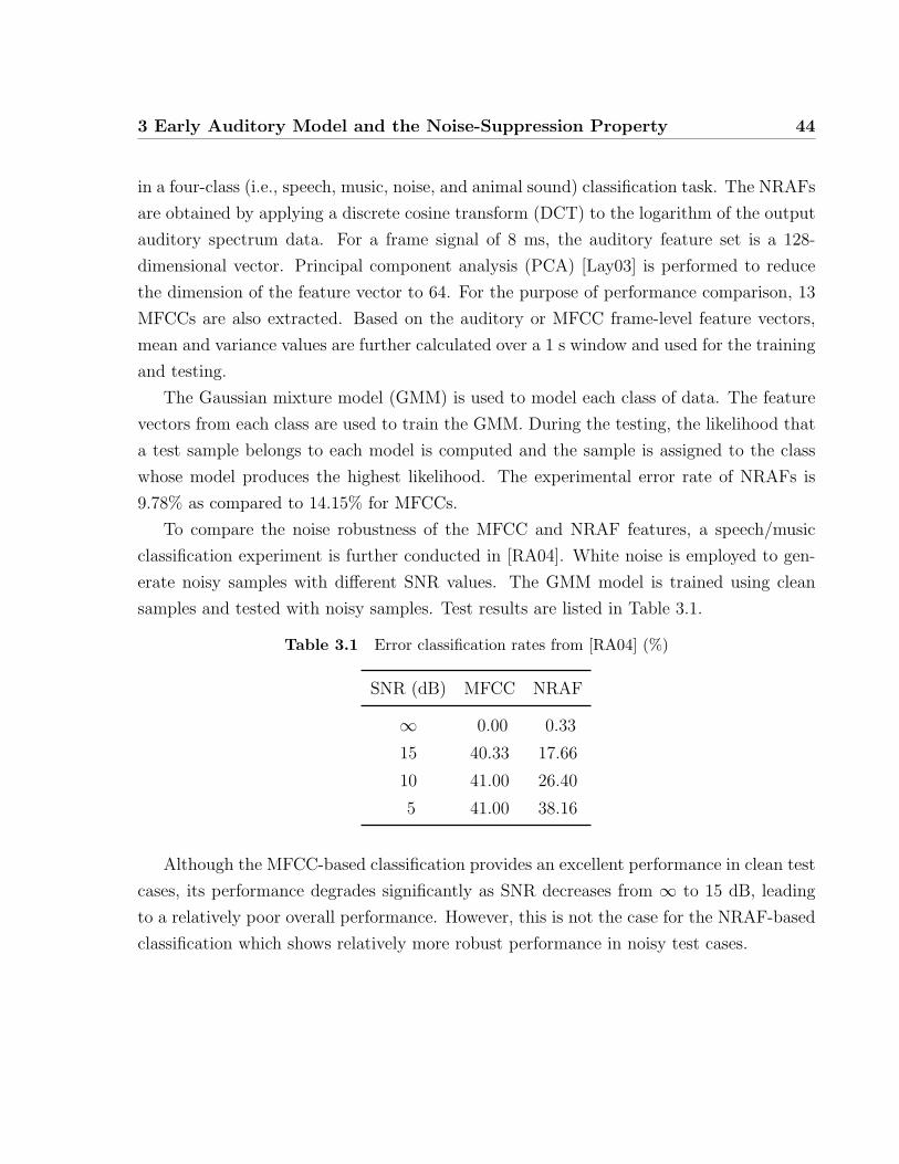
3 Early Auditory Model and the Noise-Suppression Property 44
in a four-class (i.e., speech, music, noise, and animal sound) classification task. The NRAFs
are obtained by applying a discrete cosine transform (DCT) to the logarithm of the output
auditory spectrum data. For a frame signal of 8 ms, the auditory feature set is a 128-
dimensional vector. Principal component analysis (PCA) [Lay03] is performed to reduce
the dimension of the feature vector to 64. For the purpose of performance comparison, 13
MFCCs are also extracted. Based on the auditory or MFCC frame-level feature vectors,
mean and variance values are further calculated over a 1 s window and used for the training
and testing.
The Gaussian mixture model (GMM) is used to model each class of data. The feature
vectors from each class are used to train the GMM. During the testing, the likelihood that
a test sample belongs to each model is computed and the sample is assigned to the class
whose model produces the highest likelihood. The experimental error rate of NRAFs is
9.78% as compared to 14.15% for MFCCs.
To compare the noise robustness of the MFCC and NRAF features, a speech/music
classification experiment is further conducted in [RA04]. White noise is employed to gen-
erate noisy samples with different SNR values. The GMM model is trained using clean
samples and tested with noisy samples. Test results are listed in Table 3.1.
Table 3.1 Error classification rates from [RA04] (%)
SNR (dB) MFCC NRAF
∞ 0.00 0.33
15 40.33 17.66
10 41.00 26.40
5 41.00 38.16
Although the MFCC-based classification provides an excellent performance in clean test
cases, its performance degrades significantly as SNR decreases from ∞ to 15 dB, leading
to a relatively poor overall performance. However, this is not the case for the NRAF-based
classification which shows relatively more robust performance in noisy test cases.
3 Early Auditory Model and the Noise-Suppression Property 45
3.4 Open Research Problems
Noise-robustness is a property that is lacking in many of today’s audio classification and
speech recognition systems. Inspired by the noise-suppression property of the EA model
[WS94], we seek in this thesis to investigate the application of this property to audio
classification algorithms. A series of related research topics, which are either new or have
only raised limited attention at this stage, are listed below: they form the basis of our
proposed study on auditory-based noise-robust audio classification algorithms.
Stochastic Analysis of Self-Normalization
In [WS94], the conclusions on the self-normalization property of the EA model, which
translates into spectral enhancement or noise suppression, are obtained using a qualitative
analysis first, followed by a quantitative analysis wherein a closed-form expression of the
auditory spectrum is derived. However, for the quantitative analysis, only a special, simpli-
fied case has been studied wherein a step function is used to replace the original nonlinear
sigmoid compression function. With respect to the limitation of the quantitative analysis
in [WS94], it is of interest to investigate the noise-suppression property from a broader
perspective, i.e., to derive a closed-form expression for auditory spectrum using a more
general sigmoid-like function, and to conduct relevant analysis.
Simplification/Approximation of the Original Auditory Spectrum
The noise-robustness of the original auditory spectrum has been demonstrated in different
applications [WS94, RA04]. However, this EA model is characterized by high computa-
tional requirements and nonlinear processing, which may prevent its use in some practical
applications. It is therefore desirable to compute an approximated or simplified version
of the auditory spectrum in the frequency domain wherein efficient FFT algorithms are
available. The aim is to develop a simplified FFT-based spectrum which is noise-robust in
audio classification applications while much simpler in computation, as compared to the
original auditory spectrum.
3 Early Auditory Model and the Noise-Suppression Property 46
Multi-Class Audio Classification Experiment
The effect of background noise on the performance of classification has been investigated
in [RA04] wherein a two-class classification task (i.e., speech/music) was carried out. To
evaluate the noise-robustness of a classification algorithm, a multi-class classification task,
especially with noise included as one audio class, would be more appropriate. With noise
as the background of speech or music and as one audio class, the classifier will face a more
difficult task. In addition, it is desirable to conduct classification experiments using audio
samples with different sampling frequency values.
Different features have been proposed for audio classification tasks. Considering the
focus of this research, it is of interest to extract the conventional audio features based on
the proposed approximated or simplified noise-robust FFT-based auditory spectrum.
Some other issues are also to be investigated in order to evaluate the noise-robustness of
the proposed audio classification algorithm. For example, the use of different classification
approaches, the length of audio clips, etc.
3.5 Conclusion
In this chapter, we have presented a brief introduction to the EA model [WS94], including
its processing structure, its inherent self-normalization property, and the summary of a
recent study using this model for audio classification tasks. Several research topics were
further discussed, which form the basis of our proposed study on auditory-based noise-
robust audio classification algorithms.

3 Early Auditory Model and the Noise-Suppression Property 47
48
Chapter 4
Analysis of the Self-Normalization
Property
In [WS94], a special case was investigated wherein a simplified auditory spectrum was
derived by using a step function to approximate the original sigmoid compression function
of the EA model in Fig. 3.1. Although we may take a step function as a very special case
of the sigmoid compression function, it is desirable to obtain the closed-form expression
of E[y4(t, s)] from (3.9) using a better, yet mathematically tractable, approximation. In
particular, it is of interest to determine whether the resulting expression still supports the
original qualitative analysis on self-normalization.
Having noticed the general nonlinear compression nature of the Gaussian cumulative
distribution function, and the resemblance between the graph of the sigmoid function and
that of the Gaussian CDF, below, we use the latter as an approximation to the sigmoid
compression function to derive a new closed-form expression of E[y4(t, s)] and conduct
relevant analysis.
4.1 Gaussian CDF and Sigmoid Compression Function
Referring to Fig. 3.1, the sigmoid compression function at the hair cells stage used in the
implementation [Neu] takes the following form:
g(x) =1
1 + e−x/α(4.1)
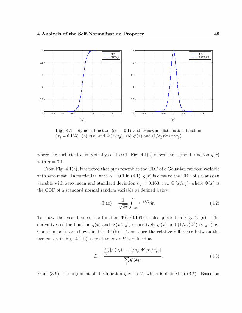
4 Analysis of the Self-Normalization Property 49
−2 −1.5 −1 −0.5 0 0.5 1 1.5 20
0.2
0.4
0.6
0.8
1g(x)Φ(x/σ
g)
(a)
−2 −1.5 −1 −0.5 0 0.5 1 1.5 20
0.5
1
1.5
2
2.5g’(x)Φ’(x/σ
g)/σ
g
(b)
Fig. 4.1 Sigmoid function (α = 0.1) and Gaussian distribution function(σg = 0.163). (a) g(x) and Φ (x/σg). (b) g′(x) and (1/σg)Φ′ (x/σg).
where the coefficient α is typically set to 0.1. Fig. 4.1(a) shows the sigmoid function g(x)
with α = 0.1.
From Fig. 4.1(a), it is noted that g(x) resembles the CDF of a Gaussian random variable
with zero mean. In particular, with α = 0.1 in (4.1), g(x) is close to the CDF of a Gaussian
variable with zero mean and standard deviation σg = 0.163, i.e., Φ (x/σg), where Φ(x) is
the CDF of a standard normal random variable as defined below:
Φ (x) =1√2π
∫ x
−∞e−t
2/2dt. (4.2)
To show the resemblance, the function Φ (x/0.163) is also plotted in Fig. 4.1(a). The
derivatives of the function g(x) and Φ (x/σg), respectively g′(x) and (1/σg)Φ′ (x/σg) (i.e.,
Gaussian pdf), are shown in Fig. 4.1(b). To measure the relative difference between the
two curves in Fig. 4.1(b), a relative error E is defined as
E =
∑i
|g′(xi)− (1/σg)Φ′(xi/σg)|∑
i
g′(xi). (4.3)
From (3.9), the argument of the function g(x) is U , which is defined in (3.7). Based on
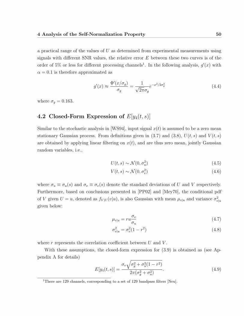
4 Analysis of the Self-Normalization Property 50
a practical range of the values of U as determined from experimental measurements using
signals with different SNR values, the relative error E between these two curves is of the
order of 5% or less for different processing channels1. In the following analysis, g′(x) with
α = 0.1 is therefore approximated as
g′(x) ≈ Φ′(x/σg)
σg=
1√2πσg
e−x2/2σ2
g (4.4)
where σg = 0.163.
4.2 Closed-Form Expression of E[y4(t, s)]
Similar to the stochastic analysis in [WS94], input signal x(t) is assumed to be a zero mean
stationary Gaussian process. From definitions given in (3.7) and (3.8), U(t, s) and V (t, s)
are obtained by applying linear filtering on x(t), and are thus zero mean, jointly Gaussian
random variables, i.e.,
U(t, s) ∼ N (0, σ2u) (4.5)
V (t, s) ∼ N (0, σ2v) (4.6)
where σu ≡ σu(s) and σv ≡ σv(s) denote the standard deviations of U and V respectively.
Furthermore, based on conclusions presented in [PP02] and [Mey70], the conditional pdf
of V given U = u, denoted as fV |U(v|u), is also Gaussian with mean µv|u and variance σ2v|u
given below:
µv|u = ruσvσu
(4.7)
σ2v|u = σ2
v(1− r2) (4.8)
where r represents the correlation coefficient between U and V .
With these assumptions, the closed-form expression for (3.9) is obtained as (see Ap-
pendix A for details)
E[y4(t, s)] =σv√σ2g + σ2
u(1− r2)
2π(σ2g + σ2
u). (4.9)
1There are 129 channels, corresponding to a set of 129 bandpass filters [Neu].
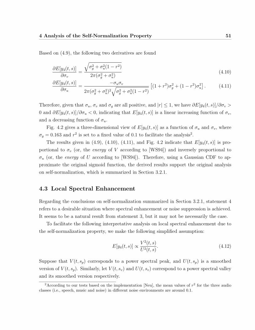
4 Analysis of the Self-Normalization Property 51
Based on (4.9), the following two derivatives are found
∂E[y4(t, s)]
∂σv=
√σ2g + σ2
u(1− r2)
2π(σ2g + σ2
u)(4.10)
∂E[y4(t, s)]
∂σu=
−σuσv2π(σ2
g + σ2u)
2√σ2g + σ2
u(1− r2)
[(1 + r2)σ2
g + (1− r2)σ2u
]. (4.11)
Therefore, given that σu, σv and σg are all positive, and |r| ≤ 1, we have ∂E[y4(t, s)]/∂σv >
0 and ∂E[y4(t, s)]/∂σu < 0, indicating that E[y4(t, s)] is a linear increasing function of σv,
and a decreasing function of σu.
Fig. 4.2 gives a three-dimensional view of E[y4(t, s)] as a function of σu and σv, where
σg = 0.163 and r2 is set to a fixed value of 0.1 to facilitate the analysis2.
The results given in (4.9), (4.10), (4.11), and Fig. 4.2 indicate that E[y4(t, s)] is pro-
portional to σv (or, the energy of V according to [WS94]) and inversely proportional to
σu (or, the energy of U according to [WS94]). Therefore, using a Gaussian CDF to ap-
proximate the original sigmoid function, the derived results support the original analysis
on self-normalization, which is summarized in Section 3.2.1.
4.3 Local Spectral Enhancement
Regarding the conclusions on self-normalization summarized in Section 3.2.1, statement 4
refers to a desirable situation where spectral enhancement or noise suppression is achieved.
It seems to be a natural result from statement 3, but it may not be necessarily the case.
To facilitate the following interpretative analysis on local spectral enhancement due to
the self-normalization property, we make the following simplified assumption:
E[y4(t, s)] ∝ V 2(t, s)
U2(t, s). (4.12)
Suppose that V (t, sp) corresponds to a power spectral peak, and U(t, sp) is a smoothed
version of V (t, sp). Similarly, let V (t, sv) and U(t, sv) correspond to a power spectral valley
and its smoothed version respectively.
2According to our tests based on the implementation [Neu], the mean values of r2 for the three audioclasses (i.e., speech, music and noise) in different noise environments are around 0.1.
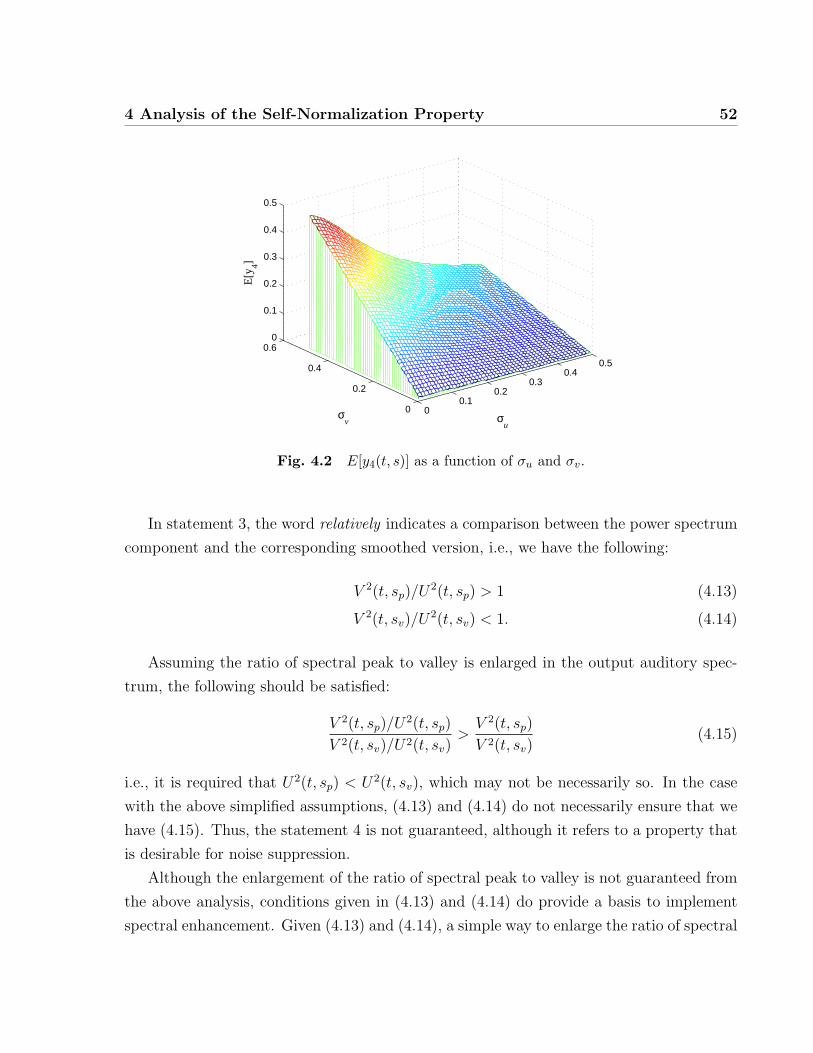
4 Analysis of the Self-Normalization Property 52
00.1
0.20.3
0.40.5
0
0.2
0.4
0.60
0.1
0.2
0.3
0.4
0.5
σu
σv
E[y
4]
Fig. 4.2 E[y4(t, s)] as a function of σu and σv.
In statement 3, the word relatively indicates a comparison between the power spectrum
component and the corresponding smoothed version, i.e., we have the following:
V 2(t, sp)/U2(t, sp) > 1 (4.13)
V 2(t, sv)/U2(t, sv) < 1. (4.14)
Assuming the ratio of spectral peak to valley is enlarged in the output auditory spec-
trum, the following should be satisfied:
V 2(t, sp)/U2(t, sp)
V 2(t, sv)/U2(t, sv)>V 2(t, sp)
V 2(t, sv)(4.15)
i.e., it is required that U2(t, sp) < U2(t, sv), which may not be necessarily so. In the case
with the above simplified assumptions, (4.13) and (4.14) do not necessarily ensure that we
have (4.15). Thus, the statement 4 is not guaranteed, although it refers to a property that
is desirable for noise suppression.
Although the enlargement of the ratio of spectral peak to valley is not guaranteed from
the above analysis, conditions given in (4.13) and (4.14) do provide a basis to implement
spectral enhancement. Given (4.13) and (4.14), a simple way to enlarge the ratio of spectral
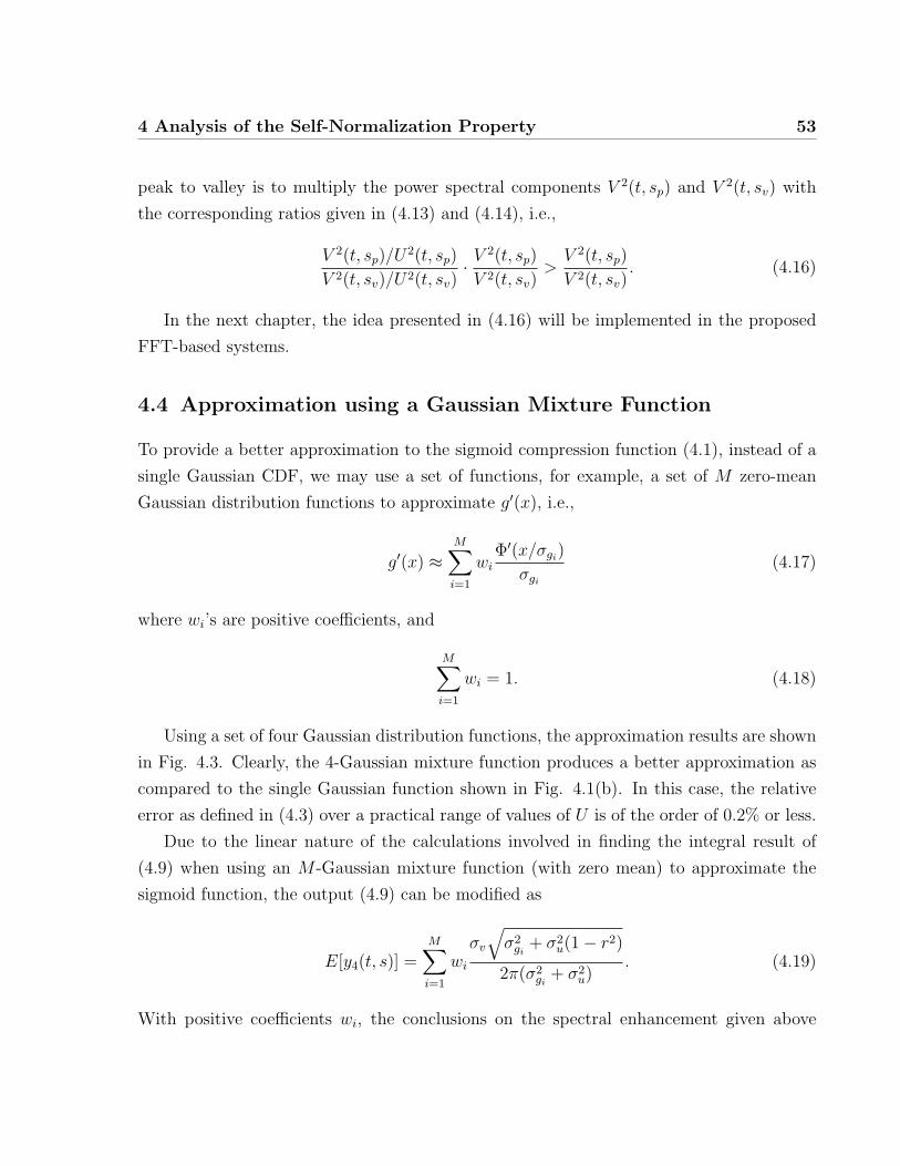
4 Analysis of the Self-Normalization Property 53
peak to valley is to multiply the power spectral components V 2(t, sp) and V 2(t, sv) with
the corresponding ratios given in (4.13) and (4.14), i.e.,
V 2(t, sp)/U2(t, sp)
V 2(t, sv)/U2(t, sv)· V
2(t, sp)
V 2(t, sv)>V 2(t, sp)
V 2(t, sv). (4.16)
In the next chapter, the idea presented in (4.16) will be implemented in the proposed
FFT-based systems.
4.4 Approximation using a Gaussian Mixture Function
To provide a better approximation to the sigmoid compression function (4.1), instead of a
single Gaussian CDF, we may use a set of functions, for example, a set of M zero-mean
Gaussian distribution functions to approximate g′(x), i.e.,
g′(x) ≈M∑i=1
wiΦ′(x/σgi)
σgi(4.17)
where wi’s are positive coefficients, and
M∑i=1
wi = 1. (4.18)
Using a set of four Gaussian distribution functions, the approximation results are shown
in Fig. 4.3. Clearly, the 4-Gaussian mixture function produces a better approximation as
compared to the single Gaussian function shown in Fig. 4.1(b). In this case, the relative
error as defined in (4.3) over a practical range of values of U is of the order of 0.2% or less.
Due to the linear nature of the calculations involved in finding the integral result of
(4.9) when using an M -Gaussian mixture function (with zero mean) to approximate the
sigmoid function, the output (4.9) can be modified as
E[y4(t, s)] =M∑i=1
wiσv√σ2gi
+ σ2u(1− r2)
2π(σ2gi
+ σ2u)
. (4.19)
With positive coefficients wi, the conclusions on the spectral enhancement given above
4 Analysis of the Self-Normalization Property 54
−2 −1.5 −1 −0.5 0 0.5 1 1.5 20
0.5
1
1.5
2
2.5g’(x)4−Gaussian
Fig. 4.3 Sigmoid function (α = 0.1) and Gaussian mixture function (M =4).
using a single Gaussian function can now be extended straightforwardly, i.e., E[y4(t, s)]
is a weighted summation of M components, with each component proportional to σv and
inversely proportional to σu.
4.5 Conclusion
In this chapter, we have used the Gaussian CDF as an approximation to the sigmoid
compression function to derive a closed-form expression of E[y4(t, s)]. Based on the derived
results, E[y4(t, s)] is proportional to the energy of V and inversely proportional to the energy
of U , which supports the original analysis on self-normalization given in [WS94]. In the
next chapter, based on the condition given in (4.16), two algorithmic implementations will
be further proposed to evaluate this noise-suppression property in the frequency domain.
4 Analysis of the Self-Normalization Property 55
56
Chapter 5
Simplification of the Auditory
Spectrum
Despite the inherent noise-suppression property, the EA model [WS94] is characterized
by high computational requirements and nonlinear processing, which may prevent its use
in certain practical applications. It is therefore desirable to reduce the computational
complexity of this model while maintaining its noise-suppression property.
In this chapter, a simplified version of the original auditory spectrum is first proposed
wherein the processing steps are linear in the time domain except for the calculation of the
square-root value of the energy. The proposed analysis naturally leads itself to frequency-
domain approximations of the auditory spectrum in order to achieve a significant reduction
in the computational complexity. Following this, a simplified FFT-based spectrum is pro-
posed wherein a local spectral self-normalization is implemented through the use of a pair of
wide and narrow filters defined in the frequency domain. Finally, an improved implementa-
tion is further proposed to calculate a so-called simplified FFT-based auditory spectrum by
making use of the characteristic frequency (CF) values of the bandpass filter set of the EA
model [WS94] for power spectrum selection, and the use of a pair of fast and slow running
averages over the frequency axis to implement the spectral self-normalization. With the in-
troduced improvements, the proposed FFT-based auditory spectrum allows more flexibility
in the extraction of noise-robust audio features.
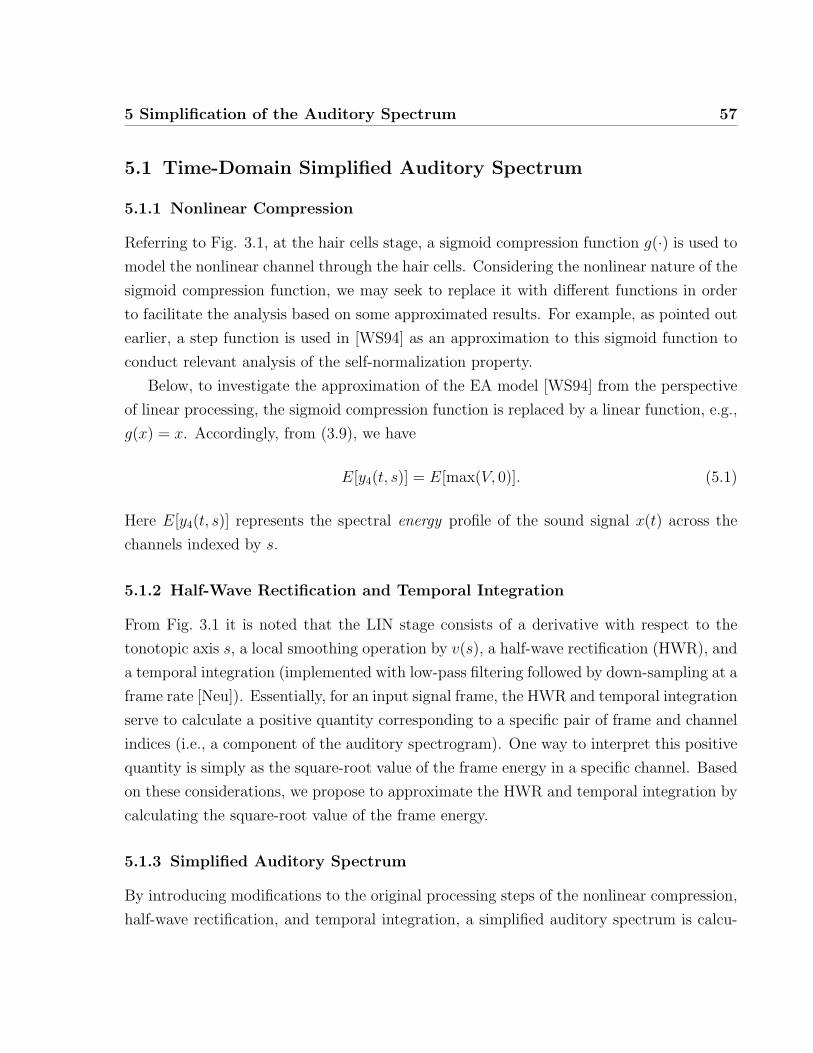
5 Simplification of the Auditory Spectrum 57
5.1 Time-Domain Simplified Auditory Spectrum
5.1.1 Nonlinear Compression
Referring to Fig. 3.1, at the hair cells stage, a sigmoid compression function g(·) is used to
model the nonlinear channel through the hair cells. Considering the nonlinear nature of the
sigmoid compression function, we may seek to replace it with different functions in order
to facilitate the analysis based on some approximated results. For example, as pointed out
earlier, a step function is used in [WS94] as an approximation to this sigmoid function to
conduct relevant analysis of the self-normalization property.
Below, to investigate the approximation of the EA model [WS94] from the perspective
of linear processing, the sigmoid compression function is replaced by a linear function, e.g.,
g(x) = x. Accordingly, from (3.9), we have
E[y4(t, s)] = E[max(V, 0)]. (5.1)
Here E[y4(t, s)] represents the spectral energy profile of the sound signal x(t) across the
channels indexed by s.
5.1.2 Half-Wave Rectification and Temporal Integration
From Fig. 3.1 it is noted that the LIN stage consists of a derivative with respect to the
tonotopic axis s, a local smoothing operation by v(s), a half-wave rectification (HWR), and
a temporal integration (implemented with low-pass filtering followed by down-sampling at a
frame rate [Neu]). Essentially, for an input signal frame, the HWR and temporal integration
serve to calculate a positive quantity corresponding to a specific pair of frame and channel
indices (i.e., a component of the auditory spectrogram). One way to interpret this positive
quantity is simply as the square-root value of the frame energy in a specific channel. Based
on these considerations, we propose to approximate the HWR and temporal integration by
calculating the square-root value of the frame energy.
5.1.3 Simplified Auditory Spectrum
By introducing modifications to the original processing steps of the nonlinear compression,
half-wave rectification, and temporal integration, a simplified auditory spectrum is calcu-
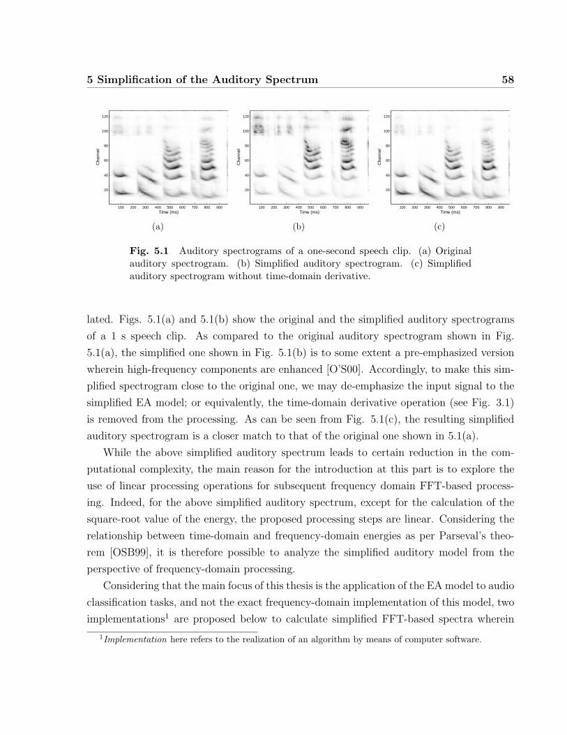
5 Simplification of the Auditory Spectrum 58
Time (ms)
Cha
nnel
100 200 300 400 500 600 700 800 900
20
40
60
80
100
120
(a)
Time (ms)
Cha
nnel
100 200 300 400 500 600 700 800 900
20
40
60
80
100
120
(b)
Time (ms)
Cha
nnel
100 200 300 400 500 600 700 800 900
20
40
60
80
100
120
(c)
Fig. 5.1 Auditory spectrograms of a one-second speech clip. (a) Originalauditory spectrogram. (b) Simplified auditory spectrogram. (c) Simplifiedauditory spectrogram without time-domain derivative.
lated. Figs. 5.1(a) and 5.1(b) show the original and the simplified auditory spectrograms
of a 1 s speech clip. As compared to the original auditory spectrogram shown in Fig.
5.1(a), the simplified one shown in Fig. 5.1(b) is to some extent a pre-emphasized version
wherein high-frequency components are enhanced [O’S00]. Accordingly, to make this sim-
plified spectrogram close to the original one, we may de-emphasize the input signal to the
simplified EA model; or equivalently, the time-domain derivative operation (see Fig. 3.1)
is removed from the processing. As can be seen from Fig. 5.1(c), the resulting simplified
auditory spectrogram is a closer match to that of the original one shown in 5.1(a).
While the above simplified auditory spectrum leads to certain reduction in the com-
putational complexity, the main reason for the introduction at this part is to explore the
use of linear processing operations for subsequent frequency domain FFT-based process-
ing. Indeed, for the above simplified auditory spectrum, except for the calculation of the
square-root value of the energy, the proposed processing steps are linear. Considering the
relationship between time-domain and frequency-domain energies as per Parseval’s theo-
rem [OSB99], it is therefore possible to analyze the simplified auditory model from the
perspective of frequency-domain processing.
Considering that the main focus of this thesis is the application of the EA model to audio
classification tasks, and not the exact frequency-domain implementation of this model, two
implementations1 are proposed below to calculate simplified FFT-based spectra wherein
1Implementation here refers to the realization of an algorithm by means of computer software.
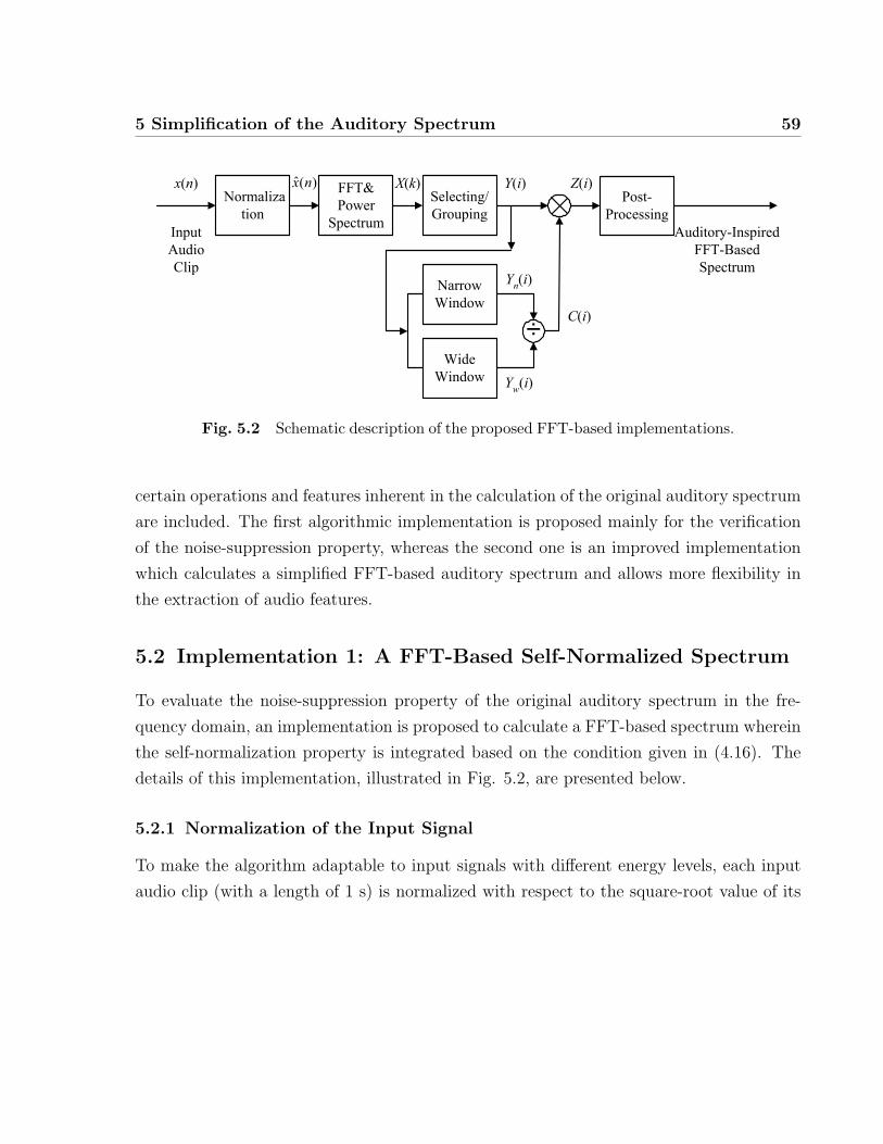
5 Simplification of the Auditory Spectrum 59
Normaliza
tion
Post-
Processing
FFT&
Power
SpectrumAuditory-Inspired
FFT-Based
Spectrum
Input
Audio
Clip
Selecting/
Grouping
X(k) Y(i)
C(i)
Wide
Window
Narrow
Window
Yn(i)
Yw(i)
Z(i)x(n) )(ˆ nx
÷
Fig. 5.2 Schematic description of the proposed FFT-based implementations.
certain operations and features inherent in the calculation of the original auditory spectrum
are included. The first algorithmic implementation is proposed mainly for the verification
of the noise-suppression property, whereas the second one is an improved implementation
which calculates a simplified FFT-based auditory spectrum and allows more flexibility in
the extraction of audio features.
5.2 Implementation 1: A FFT-Based Self-Normalized Spectrum
To evaluate the noise-suppression property of the original auditory spectrum in the fre-
quency domain, an implementation is proposed to calculate a FFT-based spectrum wherein
the self-normalization property is integrated based on the condition given in (4.16). The
details of this implementation, illustrated in Fig. 5.2, are presented below.
5.2.1 Normalization of the Input Signal
To make the algorithm adaptable to input signals with different energy levels, each input
audio clip (with a length of 1 s) is normalized with respect to the square-root value of its
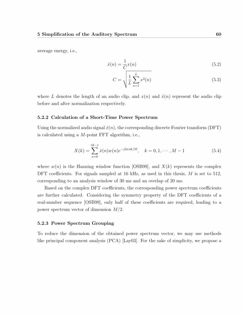
5 Simplification of the Auditory Spectrum 60
average energy, i.e.,
x(n) =1
Cx(n) (5.2)
C =
√√√√ 1
L
L∑n=1
x2(n) (5.3)
where L denotes the length of an audio clip, and x(n) and x(n) represent the audio clip
before and after normalization respectively.
5.2.2 Calculation of a Short-Time Power Spectrum
Using the normalized audio signal x(n), the corresponding discrete Fourier transform (DFT)
is calculated using a M -point FFT algorithm, i.e.,
X(k) =M−1∑n=0
x(n)w(n)e−j2πnk/M , k = 0, 1, · · · ,M − 1 (5.4)
where w(n) is the Hanning window function [OSB99], and X(k) represents the complex
DFT coefficients. For signals sampled at 16 kHz, as used in this thesis, M is set to 512,
corresponding to an analysis window of 30 ms and an overlap of 20 ms.
Based on the complex DFT coefficients, the corresponding power spectrum coefficients
are further calculated. Considering the symmetry property of the DFT coefficients of a
real-number sequence [OSB99], only half of these coefficients are required, leading to a
power spectrum vector of dimension M/2.
5.2.3 Power Spectrum Grouping
To reduce the dimension of the obtained power spectrum vector, we may use methods
like principal component analysis (PCA) [Lay03]. For the sake of simplicity, we propose a
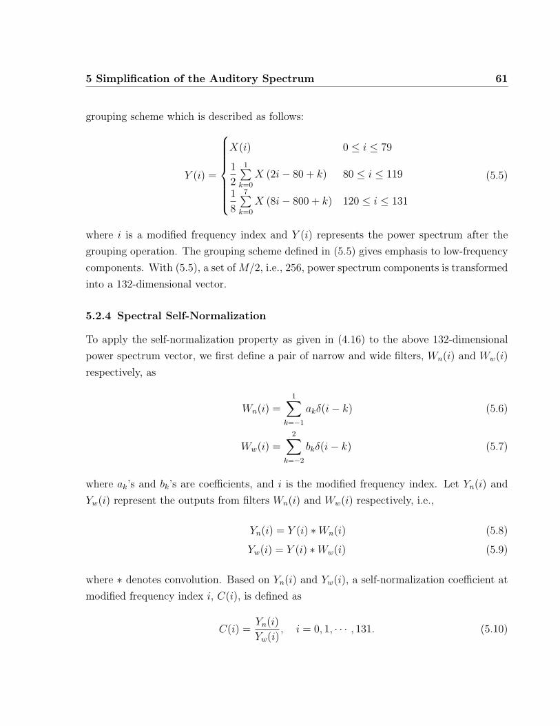
5 Simplification of the Auditory Spectrum 61
grouping scheme which is described as follows:
Y (i) =
X(i) 0 ≤ i ≤ 79
1
2
1∑k=0
X (2i− 80 + k) 80 ≤ i ≤ 119
1
8
7∑k=0
X (8i− 800 + k) 120 ≤ i ≤ 131
(5.5)
where i is a modified frequency index and Y (i) represents the power spectrum after the
grouping operation. The grouping scheme defined in (5.5) gives emphasis to low-frequency
components. With (5.5), a set of M/2, i.e., 256, power spectrum components is transformed
into a 132-dimensional vector.
5.2.4 Spectral Self-Normalization
To apply the self-normalization property as given in (4.16) to the above 132-dimensional
power spectrum vector, we first define a pair of narrow and wide filters, Wn(i) and Ww(i)
respectively, as
Wn(i) =1∑
k=−1
akδ(i− k) (5.6)
Ww(i) =2∑
k=−2
bkδ(i− k) (5.7)
where ak’s and bk’s are coefficients, and i is the modified frequency index. Let Yn(i) and
Yw(i) represent the outputs from filters Wn(i) and Ww(i) respectively, i.e.,
Yn(i) = Y (i) ∗Wn(i) (5.8)
Yw(i) = Y (i) ∗Ww(i) (5.9)
where ∗ denotes convolution. Based on Yn(i) and Yw(i), a self-normalization coefficient at
modified frequency index i, C(i), is defined as
C(i) =Yn(i)
Yw(i), i = 0, 1, · · · , 131. (5.10)
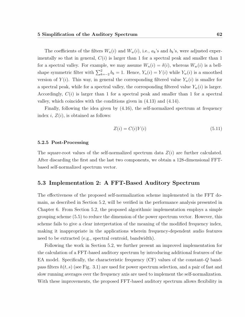
5 Simplification of the Auditory Spectrum 62
The coefficients of the filters Wn(i) and Ww(i), i.e., ak’s and bk’s, were adjusted exper-
imentally so that in general, C(i) is larger than 1 for a spectral peak and smaller than 1
for a spectral valley. For example, we may assume Wn(i) = δ(i), whereas Ww(i) is a bell-
shape symmetric filter with∑2
k=−2 bk = 1. Hence, Yn(i) = Y (i) while Yw(i) is a smoothed
version of Y (i). This way, in general the corresponding filtered value Yw(i) is smaller for
a spectral peak, while for a spectral valley, the corresponding filtered value Yw(i) is larger.
Accordingly, C(i) is larger than 1 for a spectral peak and smaller than 1 for a spectral
valley, which coincides with the conditions given in (4.13) and (4.14).
Finally, following the idea given by (4.16), the self-normalized spectrum at frequency
index i, Z(i), is obtained as follows:
Z(i) = C(i)Y (i) (5.11)
5.2.5 Post-Processing
The square-root values of the self-normalized spectrum data Z(i) are further calculated.
After discarding the first and the last two components, we obtain a 128-dimensional FFT-
based self-normalized spectrum vector.
5.3 Implementation 2: A FFT-Based Auditory Spectrum
The effectiveness of the proposed self-normalization scheme implemented in the FFT do-
main, as described in Section 5.2, will be verified in the performance analysis presented in
Chapter 6. From Section 5.2, the proposed algorithmic implementation employs a simple
grouping scheme (5.5) to reduce the dimension of the power spectrum vector. However, this
scheme fails to give a clear interpretation of the meaning of the modified frequency index,
making it inappropriate in the applications wherein frequency-dependent audio features
need to be extracted (e.g., spectral centroid, bandwidth).
Following the work in Section 5.2, we further present an improved implementation for
the calculation of a FFT-based auditory spectrum by introducing additional features of the
EA model. Specifically, the characteristic frequency (CF) values of the constant-Q band-
pass filters h(t, s) (see Fig. 3.1) are used for power spectrum selection, and a pair of fast and
slow running averages over the frequency axis are used to implement the self-normalization.
With these improvements, the proposed FFT-based auditory spectrum allows flexibility in
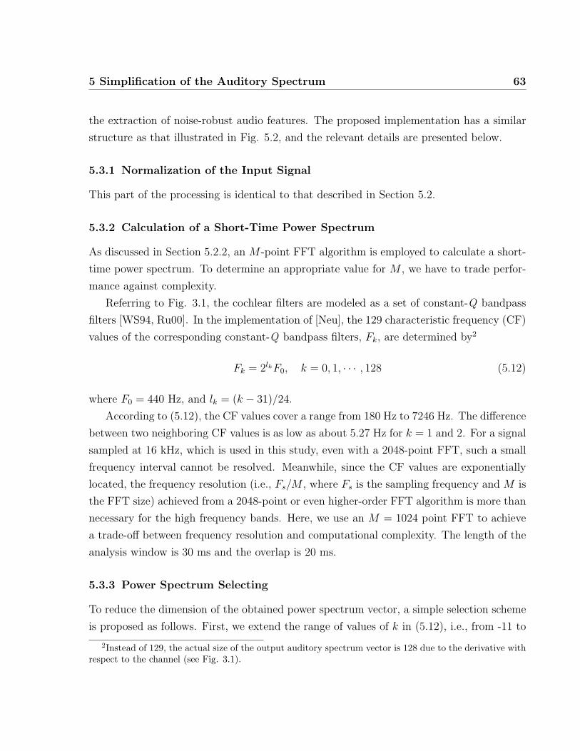
5 Simplification of the Auditory Spectrum 63
the extraction of noise-robust audio features. The proposed implementation has a similar
structure as that illustrated in Fig. 5.2, and the relevant details are presented below.
5.3.1 Normalization of the Input Signal
This part of the processing is identical to that described in Section 5.2.
5.3.2 Calculation of a Short-Time Power Spectrum
As discussed in Section 5.2.2, an M -point FFT algorithm is employed to calculate a short-
time power spectrum. To determine an appropriate value for M , we have to trade perfor-
mance against complexity.
Referring to Fig. 3.1, the cochlear filters are modeled as a set of constant-Q bandpass
filters [WS94, Ru00]. In the implementation of [Neu], the 129 characteristic frequency (CF)
values of the corresponding constant-Q bandpass filters, Fk, are determined by2
Fk = 2lkF0, k = 0, 1, · · · , 128 (5.12)
where F0 = 440 Hz, and lk = (k − 31)/24.
According to (5.12), the CF values cover a range from 180 Hz to 7246 Hz. The difference
between two neighboring CF values is as low as about 5.27 Hz for k = 1 and 2. For a signal
sampled at 16 kHz, which is used in this study, even with a 2048-point FFT, such a small
frequency interval cannot be resolved. Meanwhile, since the CF values are exponentially
located, the frequency resolution (i.e., Fs/M , where Fs is the sampling frequency and M is
the FFT size) achieved from a 2048-point or even higher-order FFT algorithm is more than
necessary for the high frequency bands. Here, we use an M = 1024 point FFT to achieve
a trade-off between frequency resolution and computational complexity. The length of the
analysis window is 30 ms and the overlap is 20 ms.
5.3.3 Power Spectrum Selecting
To reduce the dimension of the obtained power spectrum vector, a simple selection scheme
is proposed as follows. First, we extend the range of values of k in (5.12), i.e., from -11 to
2Instead of 129, the actual size of the output auditory spectrum vector is 128 due to the derivative withrespect to the channel (see Fig. 3.1).
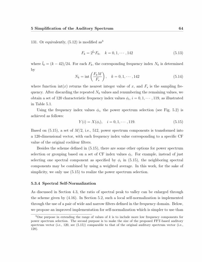
5 Simplification of the Auditory Spectrum 64
131. Or equivalently, (5.12) is modified as3
Fk = 2lkF0, k = 0, 1, · · · , 142 (5.13)
where lk = (k − 42)/24. For each Fk, the corresponding frequency index Nk is determined
by
Nk = int
(FkM
Fs
), k = 0, 1, · · · , 142 (5.14)
where function int(x) returns the nearest integer value of x, and Fs is the sampling fre-
quency. After discarding the repeated Nk values and renumbering the remaining values, we
obtain a set of 120 characteristic frequency index values φi, i = 0, 1, · · · , 119, as illustrated
in Table 5.1.
Using the frequency index values φi, the power spectrum selection (see Fig. 5.2) is
achieved as follows:
Y (i) = X(φi), i = 0, 1, · · · , 119. (5.15)
Based on (5.15), a set of M/2, i.e., 512, power spectrum components is transformed into
a 120-dimensional vector, with each frequency index value corresponding to a specific CF
value of the original cochlear filters.
Besides the scheme defined in (5.15), there are some other options for power spectrum
selection or grouping based on a set of CF index values φi. For example, instead of just
selecting one spectral component as specified by φi in (5.15), the neighboring spectral
components may be combined by using a weighted average. In this work, for the sake of
simplicity, we only use (5.15) to realize the power spectrum selection.
5.3.4 Spectral Self-Normalization
As discussed in Section 4.3, the ratio of spectral peak to valley can be enlarged through
the scheme given by (4.16). In Section 5.2, such a local self-normalization is implemented
through the use of a pair of wide and narrow filters defined in the frequency domain. Below,
we propose an improved implementation for self-normalization which is simpler to use than
3One purpose in extending the range of values of k is to include more low frequency components forpower spectrum selection. The second purpose is to make the size of the proposed FFT-based auditoryspectrum vector (i.e., 120, see (5.15)) comparable to that of the original auditory spectrum vector (i.e.,128).
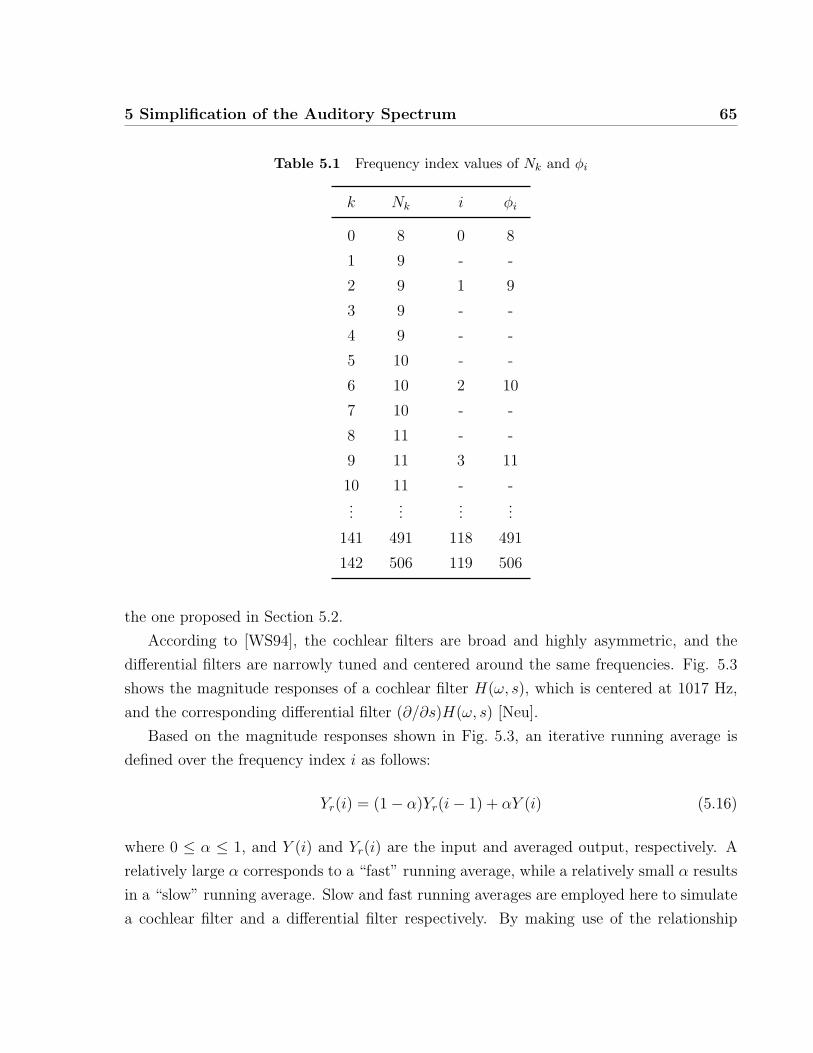
5 Simplification of the Auditory Spectrum 65
Table 5.1 Frequency index values of Nk and φi
k Nk i φi
0 8 0 8
1 9 - -
2 9 1 9
3 9 - -
4 9 - -
5 10 - -
6 10 2 10
7 10 - -
8 11 - -
9 11 3 11
10 11 - -...
......
...
141 491 118 491
142 506 119 506
the one proposed in Section 5.2.
According to [WS94], the cochlear filters are broad and highly asymmetric, and the
differential filters are narrowly tuned and centered around the same frequencies. Fig. 5.3
shows the magnitude responses of a cochlear filter H(ω, s), which is centered at 1017 Hz,
and the corresponding differential filter (∂/∂s)H(ω, s) [Neu].
Based on the magnitude responses shown in Fig. 5.3, an iterative running average is
defined over the frequency index i as follows:
Yr(i) = (1− α)Yr(i− 1) + αY (i) (5.16)
where 0 ≤ α ≤ 1, and Y (i) and Yr(i) are the input and averaged output, respectively. A
relatively large α corresponds to a “fast” running average, while a relatively small α results
in a “slow” running average. Slow and fast running averages are employed here to simulate
a cochlear filter and a differential filter respectively. By making use of the relationship
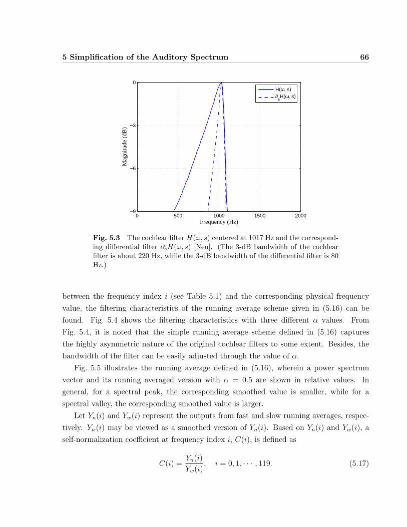
5 Simplification of the Auditory Spectrum 66
0 500 1000 1500 2000−9
−6
−3
0
Frequency (Hz)
Mag
nitu
de (
dB)
H(ω, s)∂
sH(ω, s)
Fig. 5.3 The cochlear filter H(ω, s) centered at 1017 Hz and the correspond-ing differential filter ∂sH(ω, s) [Neu]. (The 3-dB bandwidth of the cochlearfilter is about 220 Hz, while the 3-dB bandwidth of the differential filter is 80Hz.)
between the frequency index i (see Table 5.1) and the corresponding physical frequency
value, the filtering characteristics of the running average scheme given in (5.16) can be
found. Fig. 5.4 shows the filtering characteristics with three different α values. From
Fig. 5.4, it is noted that the simple running average scheme defined in (5.16) captures
the highly asymmetric nature of the original cochlear filters to some extent. Besides, the
bandwidth of the filter can be easily adjusted through the value of α.
Fig. 5.5 illustrates the running average defined in (5.16), wherein a power spectrum
vector and its running averaged version with α = 0.5 are shown in relative values. In
general, for a spectral peak, the corresponding smoothed value is smaller, while for a
spectral valley, the corresponding smoothed value is larger.
Let Yn(i) and Yw(i) represent the outputs from fast and slow running averages, respec-
tively. Yw(i) may be viewed as a smoothed version of Yn(i). Based on Yn(i) and Yw(i), a
self-normalization coefficient at frequency index i, C(i), is defined as
C(i) =Yn(i)
Yw(i), i = 0, 1, · · · , 119. (5.17)
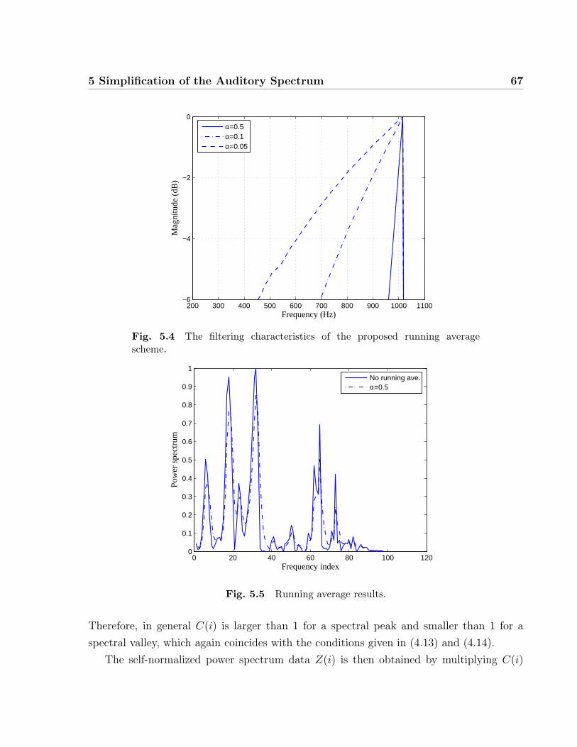
5 Simplification of the Auditory Spectrum 67
200 300 400 500 600 700 800 900 1000 1100−6
−4
−2
0
Frequency (Hz)
Mag
nitu
de (
dB)
α=0.5α=0.1α=0.05
Fig. 5.4 The filtering characteristics of the proposed running averagescheme.
0 20 40 60 80 100 1200
0.1
0.2
0.3
0.4
0.5
0.6
0.7
0.8
0.9
1
Frequency index
Pow
er s
pect
rum
No running ave.α=0.5
Fig. 5.5 Running average results.
Therefore, in general C(i) is larger than 1 for a spectral peak and smaller than 1 for a
spectral valley, which again coincides with the conditions given in (4.13) and (4.14).
The self-normalized power spectrum data Z(i) is then obtained by multiplying C(i)
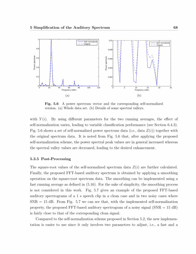
5 Simplification of the Auditory Spectrum 68
0 20 40 60 80 100 1200
0.2
0.4
0.6
0.8
1
Frequency index
Pow
er s
pect
rum
Self−normalizedOriginal
(a)
0 5 10 15 20 250
0.002
0.004
0.006
0.008
0.01
Frequency index
Pow
er s
pect
rum
Self−normalizedOriginal
(b)
Fig. 5.6 A power spectrum vector and the corresponding self-normalizedversion. (a) Whole data set. (b) Details of some spectral valleys.
with Y (i). By using different parameters for the two running averages, the effect of
self-normalization varies, leading to variable classification performance (see Section 6.4.3).
Fig. 5.6 shows a set of self-normalized power spectrum data (i.e., data Z(i)) together with
the original spectrum data. It is noted from Fig. 5.6 that, after applying the proposed
self-normalization scheme, the power spectral peak values are in general increased whereas
the spectral valley values are decreased, leading to the desired enhancement.
5.3.5 Post-Processing
The square-root values of the self-normalized spectrum data Z(i) are further calculated.
Finally, the proposed FFT-based auditory spectrum is obtained by applying a smoothing
operation on the square-root spectrum data. The smoothing can be implemented using a
fast running average as defined in (5.16). For the sake of simplicity, the smoothing process
is not considered in this work. Fig. 5.7 gives an example of the proposed FFT-based
auditory spectrograms of a 1 s speech clip in a clean case and in two noisy cases where
SNR = 15 dB. From Fig. 5.7 we can see that, with the implemented self-normalization
property, the proposed FFT-based auditory spectrogram of a noisy signal (SNR = 15 dB)
is fairly close to that of the corresponding clean signal.
Compared to the self-normalization scheme proposed in Section 5.2, the new implemen-
tation is easier to use since it only involves two parameters to adjust, i.e., a fast and a
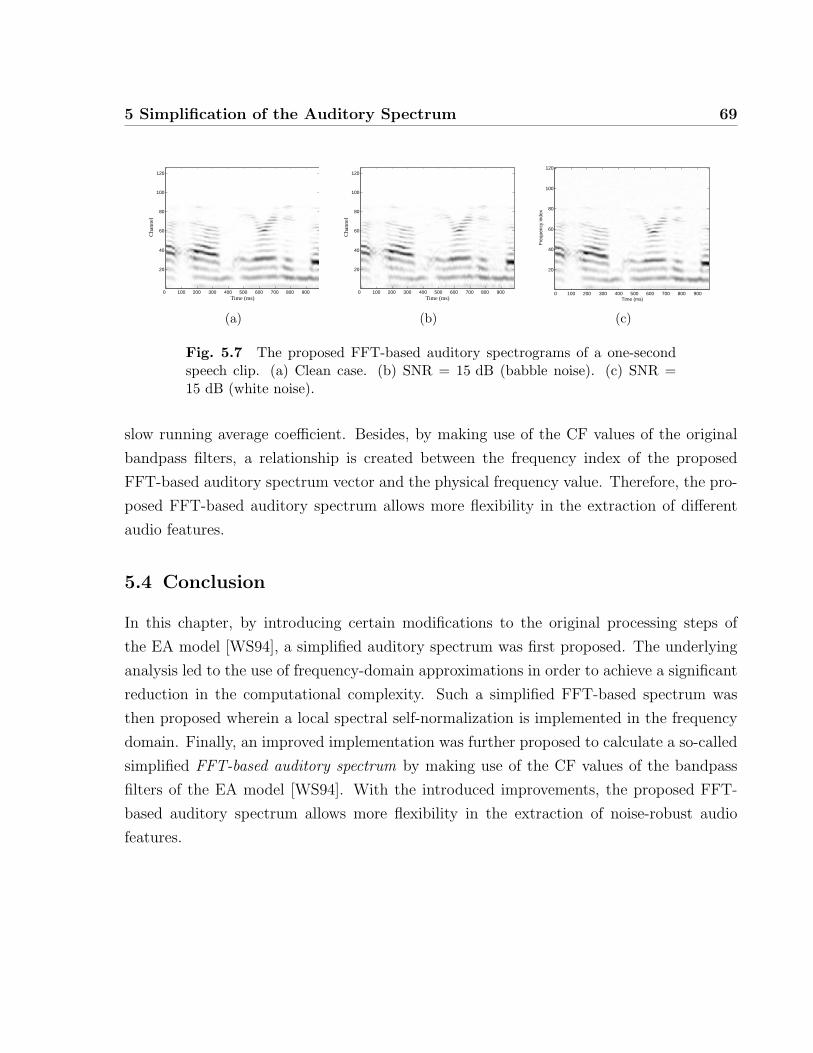
5 Simplification of the Auditory Spectrum 69
Time (ms)
Cha
nnel
0 100 200 300 400 500 600 700 800 900
20
40
60
80
100
120
(a)
Time (ms)
Cha
nnel
0 100 200 300 400 500 600 700 800 900
20
40
60
80
100
120
(b)
Time (ms)
Fre
quen
cy in
dex
0 100 200 300 400 500 600 700 800 900
20
40
60
80
100
120
(c)
Fig. 5.7 The proposed FFT-based auditory spectrograms of a one-secondspeech clip. (a) Clean case. (b) SNR = 15 dB (babble noise). (c) SNR =15 dB (white noise).
slow running average coefficient. Besides, by making use of the CF values of the original
bandpass filters, a relationship is created between the frequency index of the proposed
FFT-based auditory spectrum vector and the physical frequency value. Therefore, the pro-
posed FFT-based auditory spectrum allows more flexibility in the extraction of different
audio features.
5.4 Conclusion
In this chapter, by introducing certain modifications to the original processing steps of
the EA model [WS94], a simplified auditory spectrum was first proposed. The underlying
analysis led to the use of frequency-domain approximations in order to achieve a significant
reduction in the computational complexity. Such a simplified FFT-based spectrum was
then proposed wherein a local spectral self-normalization is implemented in the frequency
domain. Finally, an improved implementation was further proposed to calculate a so-called
simplified FFT-based auditory spectrum by making use of the CF values of the bandpass
filters of the EA model [WS94]. With the introduced improvements, the proposed FFT-
based auditory spectrum allows more flexibility in the extraction of noise-robust audio
features.
70
Chapter 6
Audio Classification Experiments
To evaluate the noise-robustness of the proposed FFT-based spectra as detailed in the
previous chapter, audio classification experiments are conducted. Below, the setup of the
audio classification experiments, including information about the audio samples, the audio
features, the classification approaches, etc., is presented first, followed by a detailed analysis
on the classification performance of different audio features.
6.1 Audio Sample Database
6.1.1 16-kHz Samples
To carry out audio classification tests, two generic audio databases are built which include
speech, music and noise clips. The sampling rate of the first audio database is 16 kHz.
This database is created for the purpose of performance comparison of all audio features
calculated in this work (see Section 6.2). A detailed description of the 16-kHz database is
given below.
• Speech: Speech clips are captured from several English web radio stations, includ-
ing CBC (the Canadian Broadcasting Corporation), BBC (the British Broadcasting
Corporation), etc. These samples are spoken by different male and female speakers
and at different speaking rates. These clips are treated as clean speech samples.
• Music: Music clips include five common types, namely: blues, classical, country, jazz,
and rock. The music clips also contain segments that are played by some Chinese
6 Audio Classification Experiments 71
traditional instruments (either alone or together with some other instruments), for
example, ruan, xiao, zheng, zhu dı, er hu, and pı pa.
The music samples used in this work include both instrumental music and vocal music
with instrumental accompaniment. These clips are treated as clean music samples.
• Noise: Noise samples are selected from the NOISEX database which contains record-
ings of various noises [VSTJMs]. A brief description of the 14 selected noise samples
is given in Table 6.1.
The total length of all these audio samples is 200 minutes, including 70 minutes of
speech, 76 minutes of music, and 54 minutes of noise. These samples are divided equally
into two parts for training and testing respectively. Three-class (speech, music and noise)
classification tests are conducted using this database to compare the performance of differ-
ent audio features. The audio classification decision is made on a one second basis.
6.1.2 8-kHz Samples
The second database is created with 8 kHz sampling frequency and used to further eval-
uate the performance of the features calculated using the proposed FFT-based auditory
spectrum, as compared to the conventional MFCC features, in a narrow-band case.
• Speech and Music: 50 minutes of speech samples and 42 minutes of music samples
are taken from the above 16-kHz database and re-sampled at 8 kHz.
• Noise: 48 minutes of noise samples are selected from an audio database provided
by the TIA/EIA/IS-727 standard [TIA98]. This standard provides minimum perfor-
mance requirements for discontinuous transmission of mobile stations operating under
the TDMA (time division multiple access) scheme. The noise samples are recorded
in four different environments. Table 6.2 gives a brief description of these noise files.
As this audio database is only used for the performance comparison between two feature
sets, namely: the conventional MFCC features and the features obtained from the proposed
FFT-based auditory spectrum, it is created with a smaller size as compared to the 16-kHz
database. In some narrow-band applications, it is desirable to have a front-end processing
unit identifying noise clips. In this thesis, noise and non-noise (i.e., speech plus music)
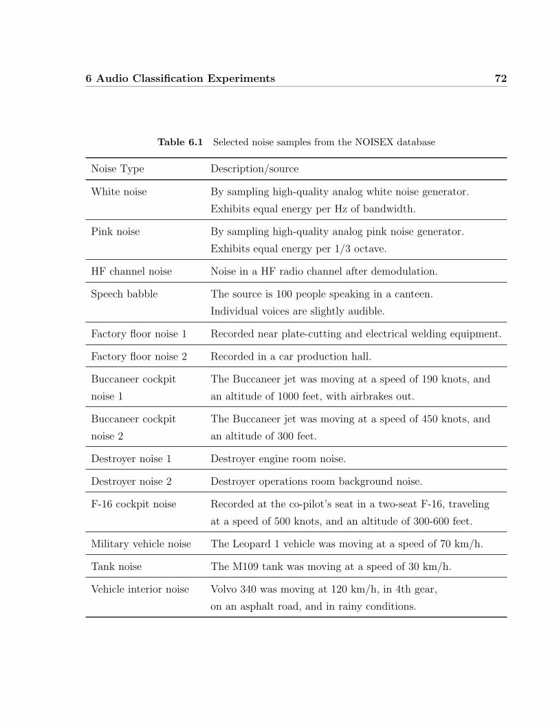
6 Audio Classification Experiments 72
Table 6.1 Selected noise samples from the NOISEX database
Noise Type Description/source
White noise By sampling high-quality analog white noise generator.
Exhibits equal energy per Hz of bandwidth.
Pink noise By sampling high-quality analog pink noise generator.
Exhibits equal energy per 1/3 octave.
HF channel noise Noise in a HF radio channel after demodulation.
Speech babble The source is 100 people speaking in a canteen.
Individual voices are slightly audible.
Factory floor noise 1 Recorded near plate-cutting and electrical welding equipment.
Factory floor noise 2 Recorded in a car production hall.
Buccaneer cockpit The Buccaneer jet was moving at a speed of 190 knots, and
noise 1 an altitude of 1000 feet, with airbrakes out.
Buccaneer cockpit The Buccaneer jet was moving at a speed of 450 knots, and
noise 2 an altitude of 300 feet.
Destroyer noise 1 Destroyer engine room noise.
Destroyer noise 2 Destroyer operations room background noise.
F-16 cockpit noise Recorded at the co-pilot’s seat in a two-seat F-16, traveling
at a speed of 500 knots, and an altitude of 300-600 feet.
Military vehicle noise The Leopard 1 vehicle was moving at a speed of 70 km/h.
Tank noise The M109 tank was moving at a speed of 30 km/h.
Vehicle interior noise Volvo 340 was moving at 120 km/h, in 4th gear,
on an asphalt road, and in rainy conditions.
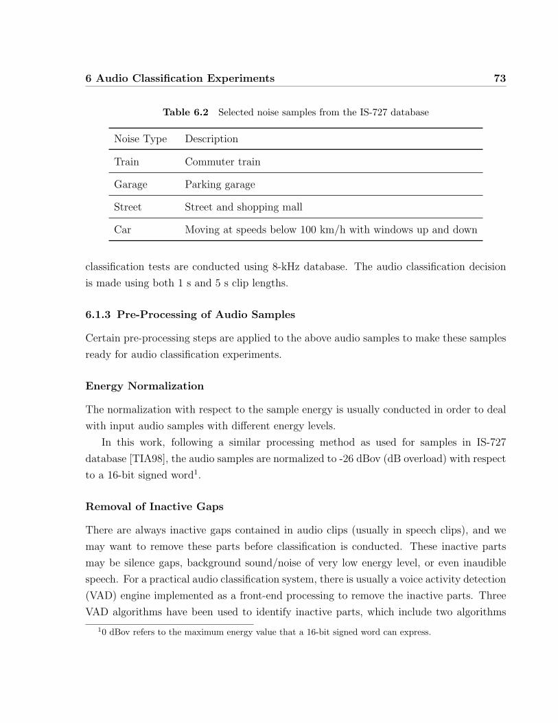
6 Audio Classification Experiments 73
Table 6.2 Selected noise samples from the IS-727 database
Noise Type Description
Train Commuter train
Garage Parking garage
Street Street and shopping mall
Car Moving at speeds below 100 km/h with windows up and down
classification tests are conducted using 8-kHz database. The audio classification decision
is made using both 1 s and 5 s clip lengths.
6.1.3 Pre-Processing of Audio Samples
Certain pre-processing steps are applied to the above audio samples to make these samples
ready for audio classification experiments.
Energy Normalization
The normalization with respect to the sample energy is usually conducted in order to deal
with input audio samples with different energy levels.
In this work, following a similar processing method as used for samples in IS-727
database [TIA98], the audio samples are normalized to -26 dBov (dB overload) with respect
to a 16-bit signed word1.
Removal of Inactive Gaps
There are always inactive gaps contained in audio clips (usually in speech clips), and we
may want to remove these parts before classification is conducted. These inactive parts
may be silence gaps, background sound/noise of very low energy level, or even inaudible
speech. For a practical audio classification system, there is usually a voice activity detection
(VAD) engine implemented as a front-end processing to remove the inactive parts. Three
VAD algorithms have been used to identify inactive parts, which include two algorithms
10 dBov refers to the maximum energy value that a 16-bit signed word can express.
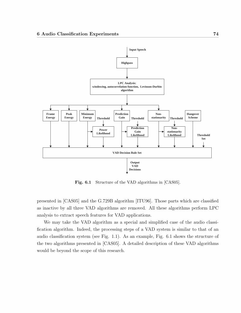
6 Audio Classification Experiments 74
Highpass
LPC Analysis: windowing, autocorrelation function, Levinson-Durbin
algorithm
Peak Energy
Minimum Energy
Prediction Gain
Prediction Gain
Likelihood
Non- stationarity Likelihood
Non- stationarity
Threshold Set
Input Speech
Threshold
Output VAD
Decisions
Hangover Scheme
Frame Energy
Power Likelihood
Threshold Threshold
VAD Decision Rule Set
Fig. 6.1 Structure of the VAD algorithms in [CAS05].
presented in [CAS05] and the G.729B algorithm [ITU96]. Those parts which are classified
as inactive by all three VAD algorithms are removed. All these algorithms perform LPC
analysis to extract speech features for VAD applications.
We may take the VAD algorithm as a special and simplified case of the audio classi-
fication algorithm. Indeed, the processing steps of a VAD system is similar to that of an
audio classification system (see Fig. 1.1). As an example, Fig. 6.1 shows the structure of
the two algorithms presented in [CAS05]. A detailed description of these VAD algorithms
would be beyond the scope of this research.
6 Audio Classification Experiments 75
6.1.4 Testing Approach
This work is focused on the development and evaluation of noise-robust audio classification
algorithms. Therefore, besides the clean samples, noisy samples with different SNR values
are also employed in our experiments. Noisy samples in each database are generated digi-
tally by adding noise segments, which are randomly selected from the corresponding noise
database, to clean speech/music segments based on long-term average energy measurement
and following specific SNR values. Specifically, we use noisy speech/music samples with
SNR values of 20, 15, 10, 5, and 0 dB.
In this work, a training or testing data set with a specific SNR value, e.g., A-dB set,
refers to a data set consisting of noisy speech and noisy music (both with SNR = A dB),
and noise only. All these samples are normalized to -26 dBov as introduced before. A
special case is the clean set wherein SNR =∞ for speech and music samples. To evaluate
the performance, audio classification experiments are conducted under both matched and
mismatched situations, which correspond to a match or a mismatch between the SNR
values of the training set and the testing set. Specifically, results from matched experiments
may reveal the interclass discriminability while results from mismatched experiments may
indicate the noise-robustness which is the main focus of this work.
6.2 Audio Features
Both frame-level and clip-level features are calculated. At the frame-level, seven sets of
audio features are calculated for performance comparison, including:
• The conventional MFCC features with and without cepstral mean subtraction (CMS).
• Conventional spectral features.
• Spectral features calculated from the FFT-based auditory spectrum (see Section 5.3).
• Discrete cosine transform (DCT)-based features computed from the original auditory
spectrum (i.e., the output of the EA model), from the FFT-based spectrum described
in Section 5.2, and from the FFT-based auditory spectrum proposed in Section 5.3.
The corresponding clip-level features are the statistical mean and variance values of
these frame-level features calculated over a time window. The details of the frame-level
features are given below.
6 Audio Classification Experiments 76
6.2.1 MFCC Features
Being widely used in the speech/speaker recognition applications, mel-frequency cepstral
coefficients (MFCCs) [RJ93, O’S00] are also useful in audio classification. For the purpose
of performance comparison, the conventional MFCCs are used in this work. A Matlab
toolbox developed by Slaney [Sla] is used to calculate a set of 13 conventional MFCCs.
As mentioned in Section 2.2.1, the mel-frequency scale is widely accepted as a linear
frequency spacing below 1000 Hz and a logarithmic spacing above 1000 Hz [DM80]. In
Slaney’s approach, the filter bank is constructed using 13 linearly-spaced filters (133.33 Hz
between center frequencies), followed by 27 log-spaced filters (with neighboring center fre-
quency values increased/decreased by a factor of 1.07) [Sla].
For conventional MFCC features, a so-called cepstral mean subtraction (CMS) tech-
nique may improve the robustness of frame-level MFCCs by removing the time averages
from the cepstrum data [Ata74]. In this work, we have used a 10 s window to calculate the
time averages of the MFCCs and to apply the CMS operation for frame-based MFCCs.
6.2.2 Spectral Features
A set of spectral features are calculated, including energy, spectral flux, spectral rolloff
point, spectral centroid, and bandwidth. Besides the conventional FFT spectrum, these
spectral features are also calculated using the FFT-based auditory spectrum proposed in
Section 5.3 in order to show its flexibility in the extraction of different audio features.
In this work, the magnitude spectrum is used to represent the “energy” instead of the
power spectrum. The magnitude spectrum is also used to calculate spectral flux, spectral
rolloff point, spectral centroid, and bandwidth (see Section 2.2 for detailed definitions of
these features).
Energy
The energy is a simple yet reliable feature for audio classification. In this work, for each
signal frame, the total energy and the energy of 3 subbands are calculated. The 3 subbands
cover frequency ranges from 0 to 1 kHz, 1 to 2 kHz and 2 to 4 kHz, respectively.
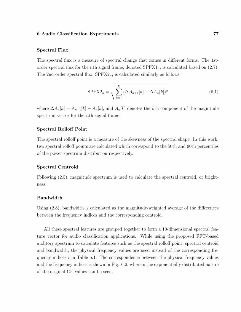
6 Audio Classification Experiments 77
Spectral Flux
The spectral flux is a measure of spectral change that comes in different forms. The 1st-
order spectral flux for the nth signal frame, denoted SPFX1n, is calculated based on (2.7).
The 2nd-order spectral flux, SPFX2n, is calculated similarly as follows:
SPFX2n =
√√√√ K∑k=1
(∆An+1[k]−∆An[k])2 (6.1)
where ∆An[k] = An+1[k]− An[k], and An[k] denotes the kth component of the magnitude
spectrum vector for the nth signal frame.
Spectral Rolloff Point
The spectral rolloff point is a measure of the skewness of the spectral shape. In this work,
two spectral rolloff points are calculated which correspond to the 50th and 90th percentiles
of the power spectrum distribution respectively.
Spectral Centroid
Following (2.5), magnitude spectrum is used to calculate the spectral centroid, or bright-
ness.
Bandwidth
Using (2.8), bandwidth is calculated as the magnitude-weighted average of the differences
between the frequency indices and the corresponding centroid.
All these spectral features are grouped together to form a 10-dimensional spectral fea-
ture vector for audio classification applications. While using the proposed FFT-based
auditory spectrum to calculate features such as the spectral rolloff point, spectral centroid
and bandwidth, the physical frequency values are used instead of the corresponding fre-
quency indices i in Table 5.1. The correspondence between the physical frequency values
and the frequency indices is shown in Fig. 6.2, wherein the exponentially distributed nature
of the original CF values can be seen.
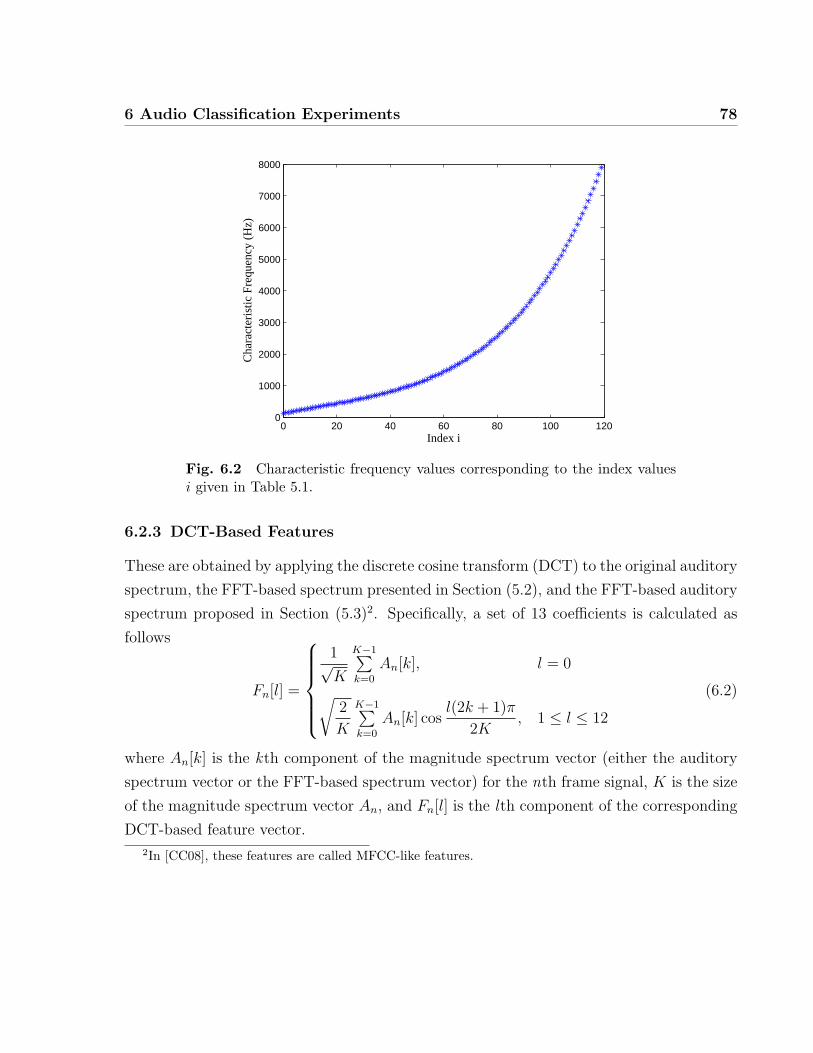
6 Audio Classification Experiments 78
0 20 40 60 80 100 1200
1000
2000
3000
4000
5000
6000
7000
8000
Index i
Cha
ract
eris
tic F
requ
ency
(H
z)
Fig. 6.2 Characteristic frequency values corresponding to the index valuesi given in Table 5.1.
6.2.3 DCT-Based Features
These are obtained by applying the discrete cosine transform (DCT) to the original auditory
spectrum, the FFT-based spectrum presented in Section (5.2), and the FFT-based auditory
spectrum proposed in Section (5.3)2. Specifically, a set of 13 coefficients is calculated as
follows
Fn[l] =
1√K
K−1∑k=0
An[k], l = 0
√2
K
K−1∑k=0
An[k] cosl(2k + 1)π
2K, 1 ≤ l ≤ 12
(6.2)
where An[k] is the kth component of the magnitude spectrum vector (either the auditory
spectrum vector or the FFT-based spectrum vector) for the nth frame signal, K is the size
of the magnitude spectrum vector An, and Fn[l] is the lth component of the corresponding
DCT-based feature vector.
2In [CC08], these features are called MFCC-like features.
6 Audio Classification Experiments 79
6.2.4 Clip-Level Features
The clip-level features used in this work are the statistical mean and variance values of the
above frame-level features calculated over a time window whose length, when otherwise
indicated, is taken to be 1 s. The clip-level features are used for the training and testing
of the classification algorithms. Table 6.3 lists all clip-level features used in this work.
From Table 6.3, the dimension of the MFCC feature sets (MFCC-CON and MFCC-CMS)
and that of the DCT-based feature sets (DCT-AUD, DCT-FFT1 and DCT-FFT2) are 26.
This reflects the fact that each of these clip-level feature sets consists of statistical mean
and variance values of the corresponding frame-level features, which are of 13 dimensions.
Similarly, the dimension of the frame-level spectral feature sets (SPEC-CON and SPEC-
FFT2) is 10, leading to the corresponding clip-level feature sets with a dimension of 20, as
given in Table 6.3.
Table 6.3 Summary of the clip-level audio features
Feature Dimension Description
MFCC-CON 26 Conventional MFCCs
MFCC-CMS 26 Conventional MFCCs with CMS operation
SPEC-CON 20 Conventional spectral features
SPEC-FFT2 20 Spectral features obtained from the FFT-based auditory
spectrum presented in Section 5.3
DCT-AUD 26 DCT-based features obtained from the original auditory
spectrum
DCT-FFT1 26 DCT-based features obtained from the FFT-based spectrum
presented in Section 5.2
DCT-FFT2 26 DCT-based features obtained from the FFT-based auditory
spectrum presented in Section 5.3
Sample distributions of 3 clip-level features, i.e., MFCC-CON, DCT-AUD and DCT-
FFT2, are shown in Figs. 6.3, 6.4 and 6.5 respectively. Considering the multi-dimensional
nature of these clip-level features, in these figures, we use only two parameters, namely:
6 Audio Classification Experiments 80
the variance values of the first and the second components of the frame-level features, to
plot two-dimensional distributions. From Figs. 6.3, 6.4 and 6.5, we may inspect both the
discriminability and the noise-robustness of the corresponding features.
Interclass Discriminability
From Figs. 6.3(a), 6.3(b) and 6.3(c), it is noted that the conventional MFCC features are
good at discriminating among three audio classes (i.e., clean speech, clean music, and noise).
There is almost no overlap between the distributions of speech and noise. For music, the
distribution overlaps with those of speech and noise. A more or less similar situation can
be found in Figs. 6.5(a), 6.5(b) and 6.5(c), which show the DCT-based features computed
from the proposed FFT-based auditory spectrum. For DCT-based features computed from
the original auditory spectrum, the discriminability is relatively lower than that of MFCC-
CON or DCT-FFT2 features (see Figs. 6.4(a), 6.4(b) and 6.4(c)).
Robustness of the Features
For MFCC-CON features, when the background noise level is increased a bit, e.g., SNR =
20 dB, relatively large changes in the distributions can be seen, for example, in Fig. 6.3(d)
as compared to Fig. 6.3(a) for speech distributions, and Fig. 6.3(g) as compared to Fig.
6.3(b) for music distributions. However, as the increase of background noise level continues,
the changes of the distributions become relatively smaller (for example, see Figs. 6.3(d),
6.3(e), and 6.3(f)). Therefore, if the SNR of the training set is 20 dB instead of the clean
set, we may expect a relatively better robustness in the testing of 15 dB and 10 dB sets.
However, when SNR = 20 dB, the discriminability is decreased compared to the clean case
as more speech feature values are now overlapped with noise feature values in the feature
space.
Comparatively, when the background noise level is increased from the clean case so that
SNR = 20 dB, DCT-AUD and DCT-FFT2 features characterize very small changes in the
distributions. For example, for DCT-AUD features, compare Figs. 6.4(a) and 6.4(d), Figs.
6.4(b) and 6.4(g); for DCT-FFT2 features, compare Figs. 6.5(a) and 6.5(d), Figs. 6.5(b)
and 6.5(g). Even when the background noise is increased to SNR = 10 dB, the changes in
the distributions of DCT-AUD and DCT-FFT2 features are still not so large as compared
to that of MFCC-CON features.
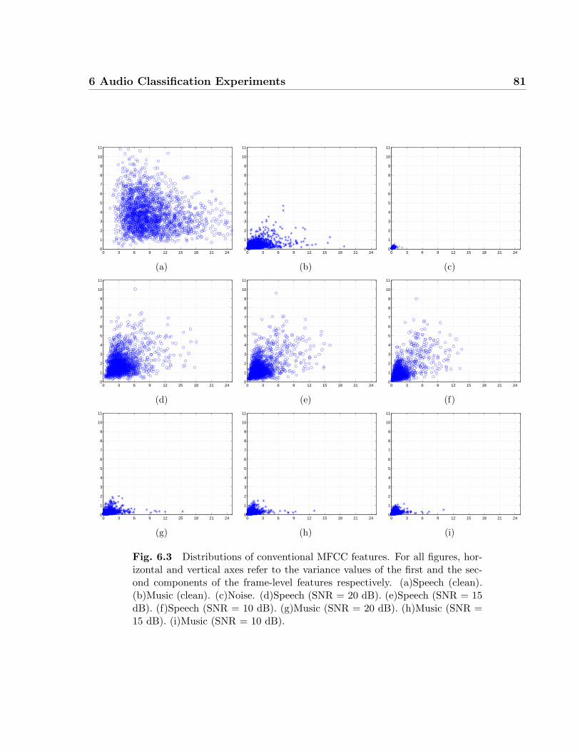
6 Audio Classification Experiments 81
0 3 6 9 12 15 18 21 240
1
2
3
4
5
6
7
8
9
10
11
(a)
0 3 6 9 12 15 18 21 240
1
2
3
4
5
6
7
8
9
10
11
(b)
0 3 6 9 12 15 18 21 240
1
2
3
4
5
6
7
8
9
10
11
(c)
0 3 6 9 12 25 18 21 240
1
2
3
4
5
6
7
8
9
10
11
(d)
0 3 6 9 12 15 18 21 240
1
2
3
4
5
6
7
8
9
10
11
(e)
0 3 6 9 12 15 18 21 240
1
2
3
4
5
6
7
8
9
10
11
(f)
0 3 6 9 12 25 18 21 240
1
2
3
4
5
6
7
8
9
10
11
(g)
0 3 6 9 12 15 18 21 240
1
2
3
4
5
6
7
8
9
10
11
(h)
0 3 6 9 12 15 18 21 240
1
2
3
4
5
6
7
8
9
10
11
(i)
Fig. 6.3 Distributions of conventional MFCC features. For all figures, hor-izontal and vertical axes refer to the variance values of the first and the sec-ond components of the frame-level features respectively. (a)Speech (clean).(b)Music (clean). (c)Noise. (d)Speech (SNR = 20 dB). (e)Speech (SNR = 15dB). (f)Speech (SNR = 10 dB). (g)Music (SNR = 20 dB). (h)Music (SNR =15 dB). (i)Music (SNR = 10 dB).
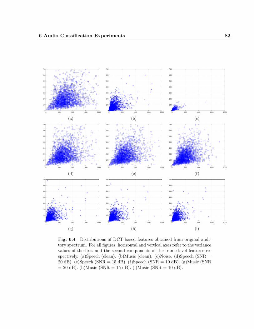
6 Audio Classification Experiments 82
0 500 1000 1500 20000
100
200
300
400
500
600
700
(a)
0 500 1000 1500 20000
100
200
300
400
500
600
700
(b)
0 500 1000 1500 20000
100
200
300
400
500
600
700
(c)
0 500 1000 1500 20000
100
200
300
400
500
600
700
(d)
0 500 1000 1500 20000
100
200
300
400
500
600
700
(e)
0 500 1000 1500 20000
100
200
300
400
500
600
700
(f)
0 500 1000 1500 20000
100
200
300
400
500
600
700
(g)
0 500 1000 1500 20000
100
200
300
400
500
600
700
(h)
0 500 1000 1500 20000
100
200
300
400
500
600
700
(i)
Fig. 6.4 Distributions of DCT-based features obtained from original audi-tory spectrum. For all figures, horizontal and vertical axes refer to the variancevalues of the first and the second components of the frame-level features re-spectively. (a)Speech (clean). (b)Music (clean). (c)Noise. (d)Speech (SNR =20 dB). (e)Speech (SNR = 15 dB). (f)Speech (SNR = 10 dB). (g)Music (SNR= 20 dB). (h)Music (SNR = 15 dB). (i)Music (SNR = 10 dB).
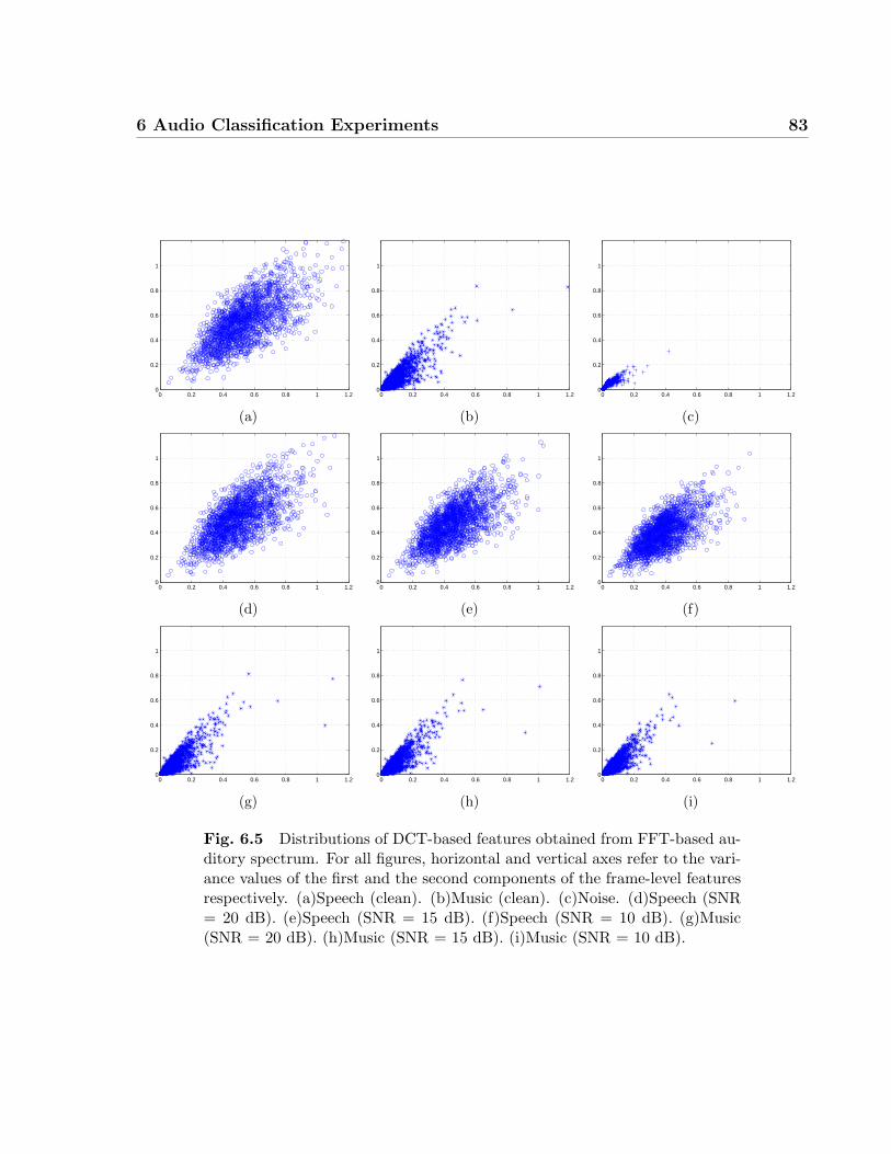
6 Audio Classification Experiments 83
0 0.2 0.4 0.6 0.8 1 1.20
0.2
0.4
0.6
0.8
1
(a)
0 0.2 0.4 0.6 0.8 1 1.20
0.2
0.4
0.6
0.8
1
(b)
0 0.2 0.4 0.6 0.8 1 1.20
0.2
0.4
0.6
0.8
1
(c)
0 0.2 0.4 0.6 0.8 1 1.20
0.2
0.4
0.6
0.8
1
(d)
0 0.2 0.4 0.6 0.8 1 1.20
0.2
0.4
0.6
0.8
1
(e)
0 0.2 0.4 0.6 0.8 1 1.20
0.2
0.4
0.6
0.8
1
(f)
0 0.2 0.4 0.6 0.8 1 1.20
0.2
0.4
0.6
0.8
1
(g)
0 0.2 0.4 0.6 0.8 1 1.20
0.2
0.4
0.6
0.8
1
(h)
0 0.2 0.4 0.6 0.8 1 1.20
0.2
0.4
0.6
0.8
1
(i)
Fig. 6.5 Distributions of DCT-based features obtained from FFT-based au-ditory spectrum. For all figures, horizontal and vertical axes refer to the vari-ance values of the first and the second components of the frame-level featuresrespectively. (a)Speech (clean). (b)Music (clean). (c)Noise. (d)Speech (SNR= 20 dB). (e)Speech (SNR = 15 dB). (f)Speech (SNR = 10 dB). (g)Music(SNR = 20 dB). (h)Music (SNR = 15 dB). (i)Music (SNR = 10 dB).
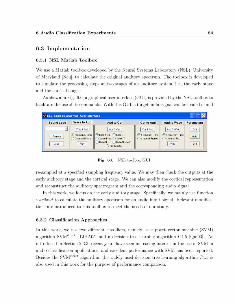
6 Audio Classification Experiments 84
6.3 Implementation
6.3.1 NSL Matlab Toolbox
We use a Matlab toolbox developed by the Neural Systems Laboratory (NSL), University
of Maryland [Neu], to calculate the original auditory spectrum. The toolbox is developed
to simulate the processing steps at two stages of an auditory system, i.e., the early stage
and the cortical stage.
As shown in Fig. 6.6, a graphical user interface (GUI) is provided by the NSL toolbox to
facilitate the use of its commands. With this GUI, a target audio signal can be loaded in and
Fig. 6.6 NSL toolbox GUI.
re-sampled at a specified sampling frequency value. We may then check the outputs at the
early auditory stage and the cortical stage. We can also modify the cortical representation
and reconstruct the auditory spectrogram and the corresponding audio signal.
In this work, we focus on the early auditory stage. Specifically, we mainly use function
wav2aud to calculate the auditory spectrum for an audio input signal. Relevant modifica-
tions are introduced to this toolbox to meet the needs of our study.
6.3.2 Classification Approaches
In this work, we use two different classifiers, namely: a support vector machine (SVM)
algorithm SVMstruct [TJHA05] and a decision tree learning algorithm C4.5 [Qui93]. As
introduced in Section 2.3.3, recent years have seen increasing interest in the use of SVM in
audio classification applications, and excellent performance with SVM has been reported.
Besides the SVMstruct algorithm, the widely used decision tree learning algorithm C4.5 is
also used in this work for the purpose of performance comparison.
6 Audio Classification Experiments 85
SVM
The SVM is a statistical learning technique that has been recently applied to audio classi-
fication applications. The SVM first transforms the input vectors into a high-dimensional
feature space using a linear or nonlinear transformation, and then conducts a linear sepa-
ration in the feature space.
SVMstruct is a specialized SVM algorithm for predicting multivariate or structured out-
puts. Unlike regular SVM algorithms that only deal with univariate prediction, SVMstruct
can predict complex objects such as trees, sequences, or sets. Examples of problems with
complex outputs include natural language parsing and sequence alignment [TJHA05]. In
this work, we use radial basis function (RBF) as the kernel function, and the model is
tuned to achieve the best training performance.
C4.5
The classification rules of the C4.5 algorithm are in the form of a decision tree, which is
built from a set of training data using the concept of information entropy [Qui93]. Given
a set of attributes which form the data vectors, C4.5 examines the so called normalized
information gain (difference in entropy) that results from choosing a specific attribute to
split the data. The attribute with the highest normalized information gain is the one used
to make the decision. A decision node is then created to split the data set to smaller
sublists. The algorithm recurs on the smaller sublists thereafter and adds the generated
nodes as children of the aforementioned node. When all samples in a sublist belong to a
same class, a leaf node can be created for the decision tree to output the corresponding
class value.
As a widely used decision tree learning algorithm, we are interested in comparing its
performance with that of the SVMstruct algorithm in audio classification applications.
6 Audio Classification Experiments 86
6.4 Performance Analysis
6.4.1 Performance Comparison with the 16-kHz Database
Case 1: Training with Clean Data Set
In this case, the training set consists of clean speech, clean music, and noise samples.
This is probably the most popular way to train a classification system. Using the 16-kHz
audio database and with SVM and C4.5 as the classifiers, speech/music/noise classification
experiments are conducted. The corresponding error testing rates as a function of SNR
values are shown in Fig. 6.7 for different audio features (see Table 6.3), wherein the total
number of audio clips under testing is 6000. To calculate the proposed FFT-based auditory
spectrum (see Section 5.3), the fast and slow running average coefficients are set to 1 and
0.5 respectively.
Table 6.4 lists error classification rates for different audio features wherein results are
presented in the following categories:
• Matched (Clean): The error rate in the matched test case, i.e., with clean set as the
testing set.
• Average-Mismatched : The average error rate in five mismatched test cases, i.e., SNR
= 20, 15, 10, 5 and 0 dB.
• Average-Overall : The overall average over the above two results.
Based on the results presented in Table 6.4 and Fig. 6.7, the following conclusions can
be reached.
• Best performance: The best overall average error rate is 10.2%, which is achieved by
the DCT-FFT2 feature set with SVM as the classifier. Besides, the DCT-FFT2 fea-
ture set together with SVM also performs best in mismatched test cases wherein the
average error rate is 18.2% whereas that of the MFCC-CON feature set is 40.6%. How-
ever, the MFCC-CON feature set together with SVM performs best in the matched
(or clean) test case with an error rate of 1.9%.
• SVM vs. C4.5 : As for the two classification approaches, results from Table 6.4 in-
dicate that SVM outperforms C4.5 in matched test case for each feature set. This
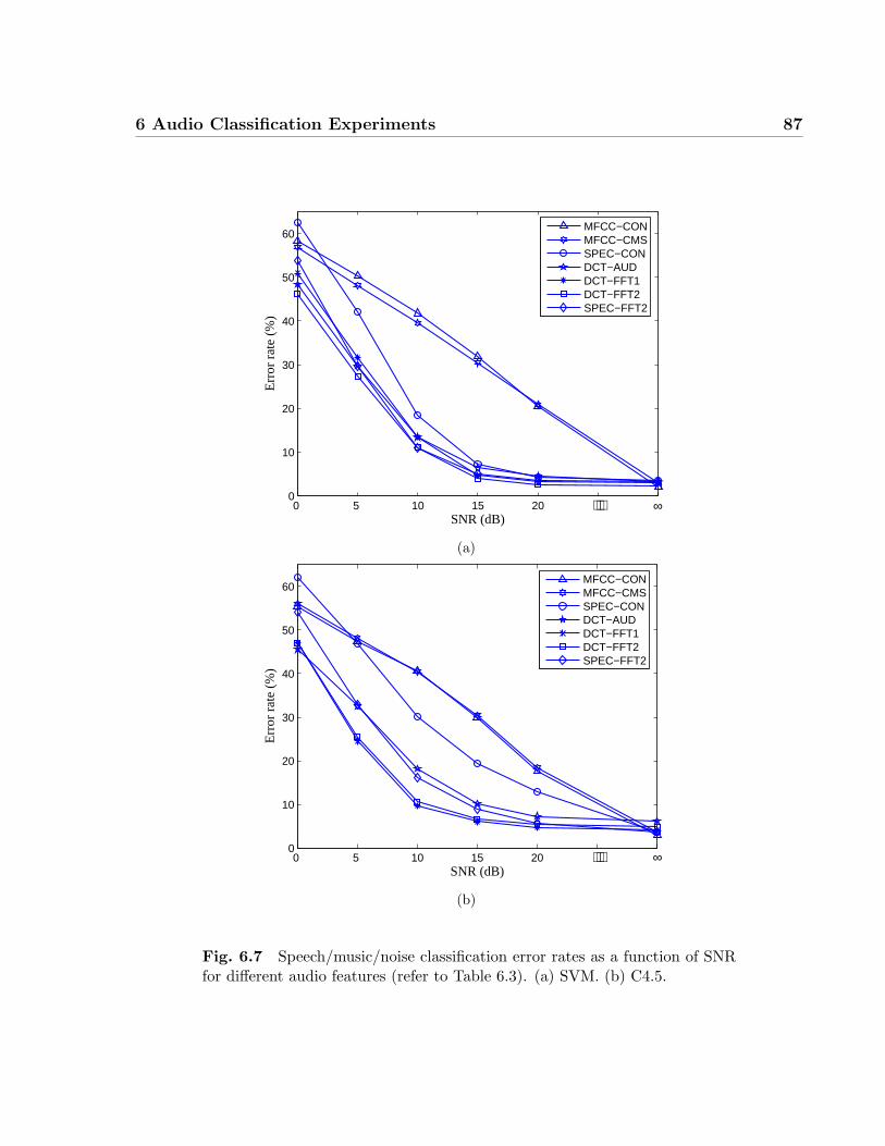
6 Audio Classification Experiments 87
0 5 10 15 200
10
20
30
40
50
60
SNR (dB)
Err
or r
ate
(%)
MFCC−CONMFCC−CMSSPEC−CONDCT−AUDDCT−FFT1DCT−FFT2SPEC−FFT2
⋅⋅⋅ ∞
(a)
0 5 10 15 200
10
20
30
40
50
60
SNR (dB)
Err
or r
ate
(%)
MFCC−CONMFCC−CMSSPEC−CONDCT−AUDDCT−FFT1DCT−FFT2SPEC−FFT2
⋅⋅⋅ ∞
(b)
Fig. 6.7 Speech/music/noise classification error rates as a function of SNRfor different audio features (refer to Table 6.3). (a) SVM. (b) C4.5.
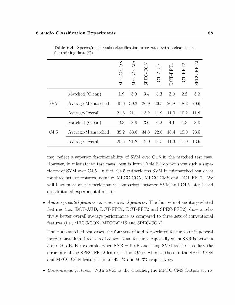
6 Audio Classification Experiments 88
Table 6.4 Speech/music/noise classification error rates with a clean set asthe training data (%)
MF
CC
-CO
N
MF
CC
-CM
S
SP
EC
-CO
N
DC
T-A
UD
DC
T-F
FT
1
DC
T-F
FT
2
SP
EC
-FF
T2
Matched (Clean) 1.9 3.0 3.4 3.3 3.0 2.2 3.2
SVM Average-Mismatched 40.6 39.2 26.9 20.5 20.8 18.2 20.6
Average-Overall 21.3 21.1 15.2 11.9 11.9 10.2 11.9
Matched (Clean) 2.8 3.6 3.6 6.2 4.1 4.8 3.6
C4.5 Average-Mismatched 38.2 38.8 34.3 22.8 18.4 19.0 23.5
Average-Overall 20.5 21.2 19.0 14.5 11.3 11.9 13.6
may reflect a superior discriminability of SVM over C4.5 in the matched test case.
However, in mismatched test cases, results from Table 6.4 do not show such a supe-
riority of SVM over C4.5. In fact, C4.5 outperforms SVM in mismatched test cases
for three sets of features, namely: MFCC-CON, MFCC-CMS and DCT-FFT1. We
will have more on the performance comparison between SVM and C4.5 later based
on additional experimental results.
• Auditory-related features vs. conventional features : The four sets of auditory-related
features (i.e., DCT-AUD, DCT-FFT1, DCT-FFT2 and SPEC-FFT2) show a rela-
tively better overall average performance as compared to three sets of conventional
features (i.e., MFCC-CON, MFCC-CMS and SPEC-CON).
Under mismatched test cases, the four sets of auditory-related features are in general
more robust than three sets of conventional features, especially when SNR is between
5 and 20 dB. For example, when SNR = 5 dB and using SVM as the classifier, the
error rate of the SPEC-FFT2 feature set is 29.7%, whereas those of the SPEC-CON
and MFCC-CON feature sets are 42.1% and 50.3% respectively.
• Conventional features : With SVM as the classifier, the MFCC-CMS feature set re-
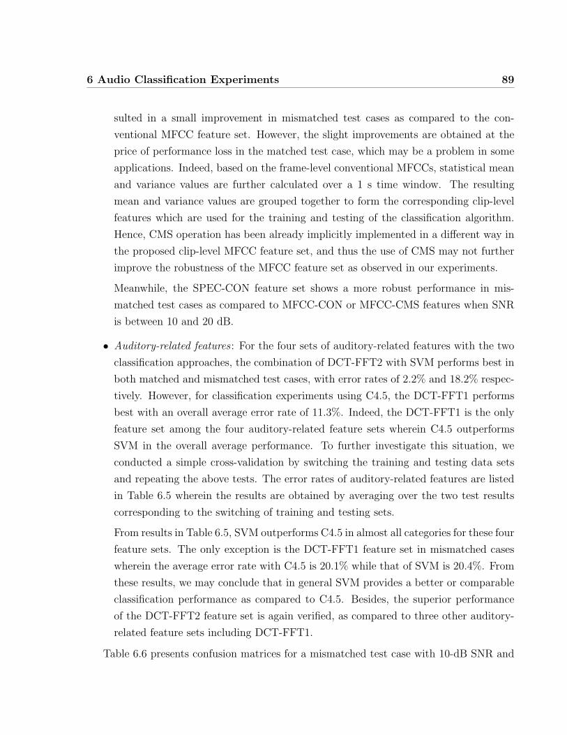
6 Audio Classification Experiments 89
sulted in a small improvement in mismatched test cases as compared to the con-
ventional MFCC feature set. However, the slight improvements are obtained at the
price of performance loss in the matched test case, which may be a problem in some
applications. Indeed, based on the frame-level conventional MFCCs, statistical mean
and variance values are further calculated over a 1 s time window. The resulting
mean and variance values are grouped together to form the corresponding clip-level
features which are used for the training and testing of the classification algorithm.
Hence, CMS operation has been already implicitly implemented in a different way in
the proposed clip-level MFCC feature set, and thus the use of CMS may not further
improve the robustness of the MFCC feature set as observed in our experiments.
Meanwhile, the SPEC-CON feature set shows a more robust performance in mis-
matched test cases as compared to MFCC-CON or MFCC-CMS features when SNR
is between 10 and 20 dB.
• Auditory-related features : For the four sets of auditory-related features with the two
classification approaches, the combination of DCT-FFT2 with SVM performs best in
both matched and mismatched test cases, with error rates of 2.2% and 18.2% respec-
tively. However, for classification experiments using C4.5, the DCT-FFT1 performs
best with an overall average error rate of 11.3%. Indeed, the DCT-FFT1 is the only
feature set among the four auditory-related feature sets wherein C4.5 outperforms
SVM in the overall average performance. To further investigate this situation, we
conducted a simple cross-validation by switching the training and testing data sets
and repeating the above tests. The error rates of auditory-related features are listed
in Table 6.5 wherein the results are obtained by averaging over the two test results
corresponding to the switching of training and testing sets.
From results in Table 6.5, SVM outperforms C4.5 in almost all categories for these four
feature sets. The only exception is the DCT-FFT1 feature set in mismatched cases
wherein the average error rate with C4.5 is 20.1% while that of SVM is 20.4%. From
these results, we may conclude that in general SVM provides a better or comparable
classification performance as compared to C4.5. Besides, the superior performance
of the DCT-FFT2 feature set is again verified, as compared to three other auditory-
related feature sets including DCT-FFT1.
Table 6.6 presents confusion matrices for a mismatched test case with 10-dB SNR and
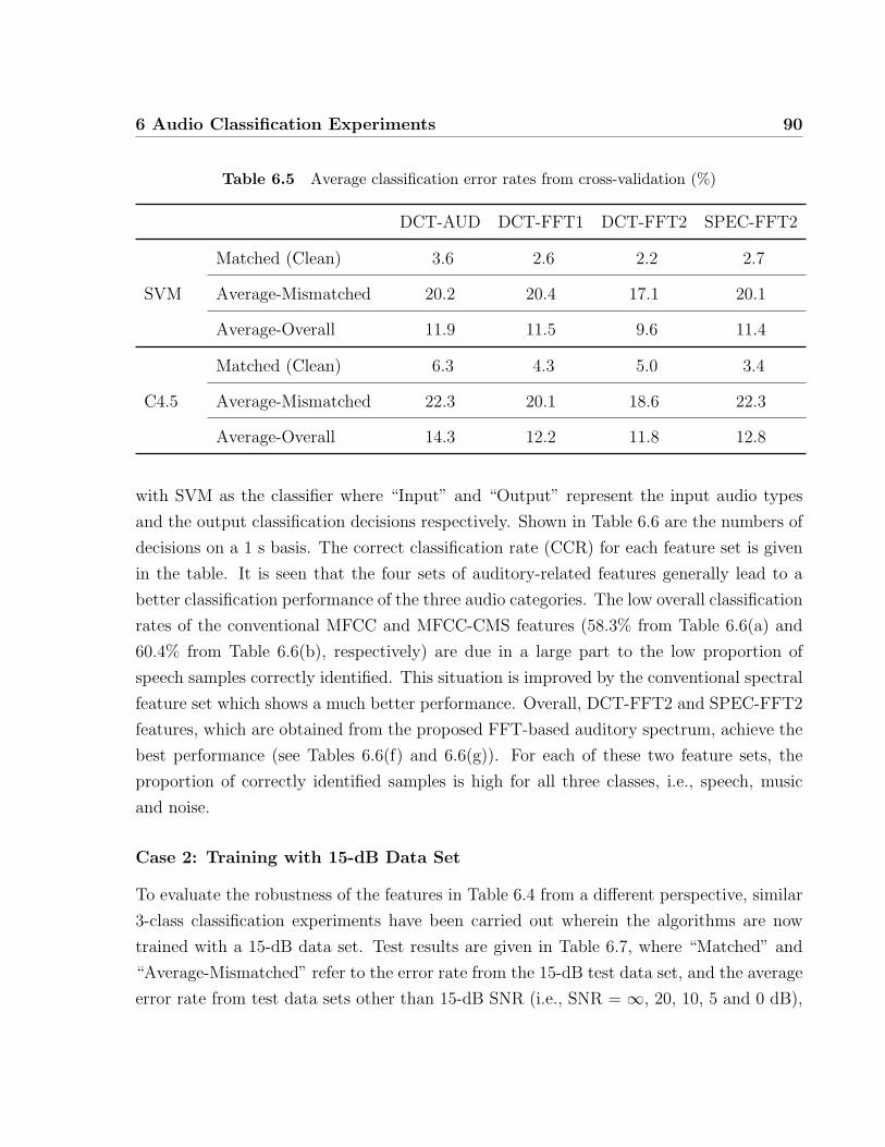
6 Audio Classification Experiments 90
Table 6.5 Average classification error rates from cross-validation (%)
DCT-AUD DCT-FFT1 DCT-FFT2 SPEC-FFT2
Matched (Clean) 3.6 2.6 2.2 2.7
SVM Average-Mismatched 20.2 20.4 17.1 20.1
Average-Overall 11.9 11.5 9.6 11.4
Matched (Clean) 6.3 4.3 5.0 3.4
C4.5 Average-Mismatched 22.3 20.1 18.6 22.3
Average-Overall 14.3 12.2 11.8 12.8
with SVM as the classifier where “Input” and “Output” represent the input audio types
and the output classification decisions respectively. Shown in Table 6.6 are the numbers of
decisions on a 1 s basis. The correct classification rate (CCR) for each feature set is given
in the table. It is seen that the four sets of auditory-related features generally lead to a
better classification performance of the three audio categories. The low overall classification
rates of the conventional MFCC and MFCC-CMS features (58.3% from Table 6.6(a) and
60.4% from Table 6.6(b), respectively) are due in a large part to the low proportion of
speech samples correctly identified. This situation is improved by the conventional spectral
feature set which shows a much better performance. Overall, DCT-FFT2 and SPEC-FFT2
features, which are obtained from the proposed FFT-based auditory spectrum, achieve the
best performance (see Tables 6.6(f) and 6.6(g)). For each of these two feature sets, the
proportion of correctly identified samples is high for all three classes, i.e., speech, music
and noise.
Case 2: Training with 15-dB Data Set
To evaluate the robustness of the features in Table 6.4 from a different perspective, similar
3-class classification experiments have been carried out wherein the algorithms are now
trained with a 15-dB data set. Test results are given in Table 6.7, where “Matched” and
“Average-Mismatched” refer to the error rate from the 15-dB test data set, and the average
error rate from test data sets other than 15-dB SNR (i.e., SNR = ∞, 20, 10, 5 and 0 dB),
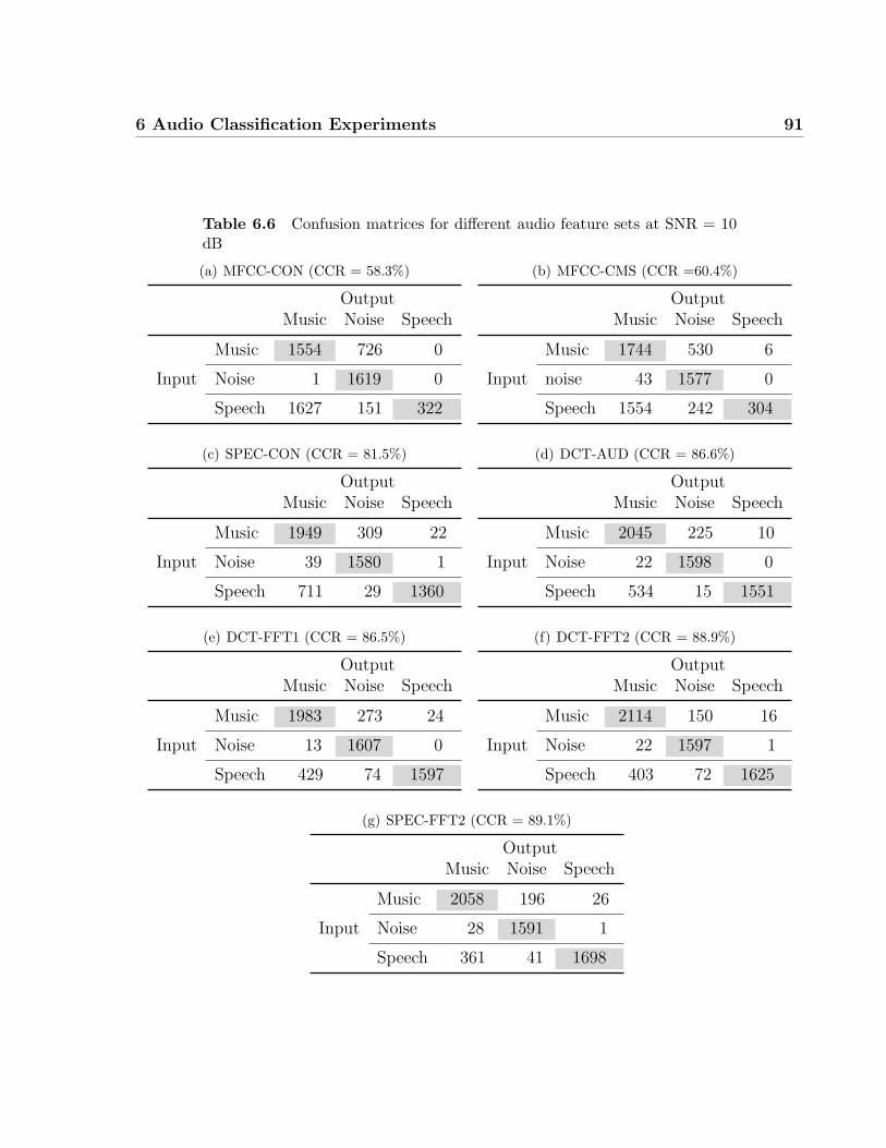
6 Audio Classification Experiments 91
Table 6.6 Confusion matrices for different audio feature sets at SNR = 10dB
(a) MFCC-CON (CCR = 58.3%)
OutputMusic Noise Speech
Music 1554 726 0
Input Noise 1 1619 0
Speech 1627 151 322
(b) MFCC-CMS (CCR =60.4%)
OutputMusic Noise Speech
Music 1744 530 6
Input noise 43 1577 0
Speech 1554 242 304
(c) SPEC-CON (CCR = 81.5%)
OutputMusic Noise Speech
Music 1949 309 22
Input Noise 39 1580 1
Speech 711 29 1360
(d) DCT-AUD (CCR = 86.6%)
OutputMusic Noise Speech
Music 2045 225 10
Input Noise 22 1598 0
Speech 534 15 1551
(e) DCT-FFT1 (CCR = 86.5%)
OutputMusic Noise Speech
Music 1983 273 24
Input Noise 13 1607 0
Speech 429 74 1597
(f) DCT-FFT2 (CCR = 88.9%)
OutputMusic Noise Speech
Music 2114 150 16
Input Noise 22 1597 1
Speech 403 72 1625
(g) SPEC-FFT2 (CCR = 89.1%)
OutputMusic Noise Speech
Music 2058 196 26
Input Noise 28 1591 1
Speech 361 41 1698
6 Audio Classification Experiments 92
respectively.
Table 6.7 Speech/music/noise classification error rates with a 15-dB set asthe training data (%)
MF
CC
-CO
N
MF
CC
-CM
S
SP
EC
-CO
N
DC
T-A
UD
DC
T-F
FT
1
DC
T-F
FT
2
SP
EC
-FF
T2
Matched (15 dB) 2.1 5.3 3.3 3.8 3.4 3.4 3.4
SVM Average-Mismatched 20.8 17.8 16.7 16.0 14.7 14.3 14.6
Matched (15 dB) 5.6 6.9 5.2 6.4 5.0 5.8 4.0
C4.5 Average-Mismatched 20.2 20.0 20.3 18.4 15.6 16.4 17.1
It is noted that in general SVM outperforms C4.5 (the only exception is the MFCC-CON
features set in mismatched tests). In the matched test case (i.e., SNR = 15 dB), MFCC-
CON with SVM again shows the best discriminability with an error rate of 2.1%, whereas
DCT-FFT2 with SVM gives the best average performance in mismatched test cases with
an average error rate of 14.3%. The performance of the 4 sets of auditory-related features
in mismatched test cases is better than that of 3 sets of conventional features; however,
compared to the results in Table 6.4, the performance gap between the auditory-related
and the conventional features becomes smaller. Indeed when the SNR of the training set
is 15 dB while that of the testing set is ∞, 20, or 10 dB, the classification performance of
these conventional features is close to that of the auditory-related features, leading to an
improved average performance in mismatched test cases as given in Table 6.7.
6.4.2 Performance Comparison with the 8-kHz Database
The robustness of the proposed FFT-based auditory spectrum has been verified by DCT-
FFT2 and SPEC-FFT2 features in the above 3-class classification experiments with an
audio database sampled at the rate of 16 kHz. To further evaluate the performance of
the proposed FFT-based auditory spectrum in a narrow-band application where the main
focus is on the identification of noise, two-class, i.e., noise/non-noise classification tests are
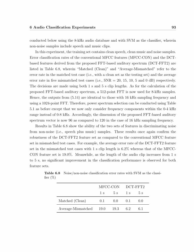
6 Audio Classification Experiments 93
conducted below using the 8-kHz audio database and with SVM as the classifier, wherein
non-noise samples include speech and music clips.
In this experiment, the training set contains clean speech, clean music and noise samples.
Error classification rates of the conventional MFCC features (MFCC-CON) and the DCT-
based features derived from the proposed FFT-based auditory spectrum (DCT-FFT2) are
listed in Table 6.8, wherein “Matched (Clean)” and “Average-Mismatched” refer to the
error rate in the matched test case (i.e., with a clean set as the testing set) and the average
error rate in five mismatched test cases (i.e., SNR = 20, 15, 10, 5 and 0 dB) respectively.
The decisions are made using both 1 s and 5 s clip lengths. As for the calculation of the
proposed FFT-based auditory spectrum, a 512-point FFT is now used for 8-kHz samples.
Hence, the outputs from (5.14) are identical to those with 16 kHz sampling frequency and
using a 1024-point FFT. Therefore, power spectrum selection can be conducted using Table
5.1 as before except that we now only consider frequency components within the 0-4 kHz
range instead of 0-8 kHz. Accordingly, the dimension of the proposed FFT-based auditory
spectrum vector is now 96 as compared to 120 in the case of 16 kHz sampling frequency.
Results in Table 6.8 show the ability of the two sets of features in discriminating noise
from non-noise (i.e., speech plus music) samples. These results once again confirm the
robustness of the DCT-FFT2 feature set as compared to the conventional MFCC feature
set in mismatched test cases. For example, the average error rate of the DCT-FFT2 feature
set in the mismatched test cases with 1 s clip length is 6.2% whereas that of the MFCC-
CON feature set is 19.0%. Meanwhile, as the length of the audio clip increases from 1 s
to 5 s, no significant improvement in the classification performance is observed for both
feature sets.
Table 6.8 Noise/non-noise classification error rates with SVM as the classi-fier (%)
MFCC-CON DCT-FFT2
1 s 5 s 1 s 5 s
Matched (Clean) 0.1 0.0 0.1 0.0
Average-Mismatched 19.0 19.3 6.2 6.1
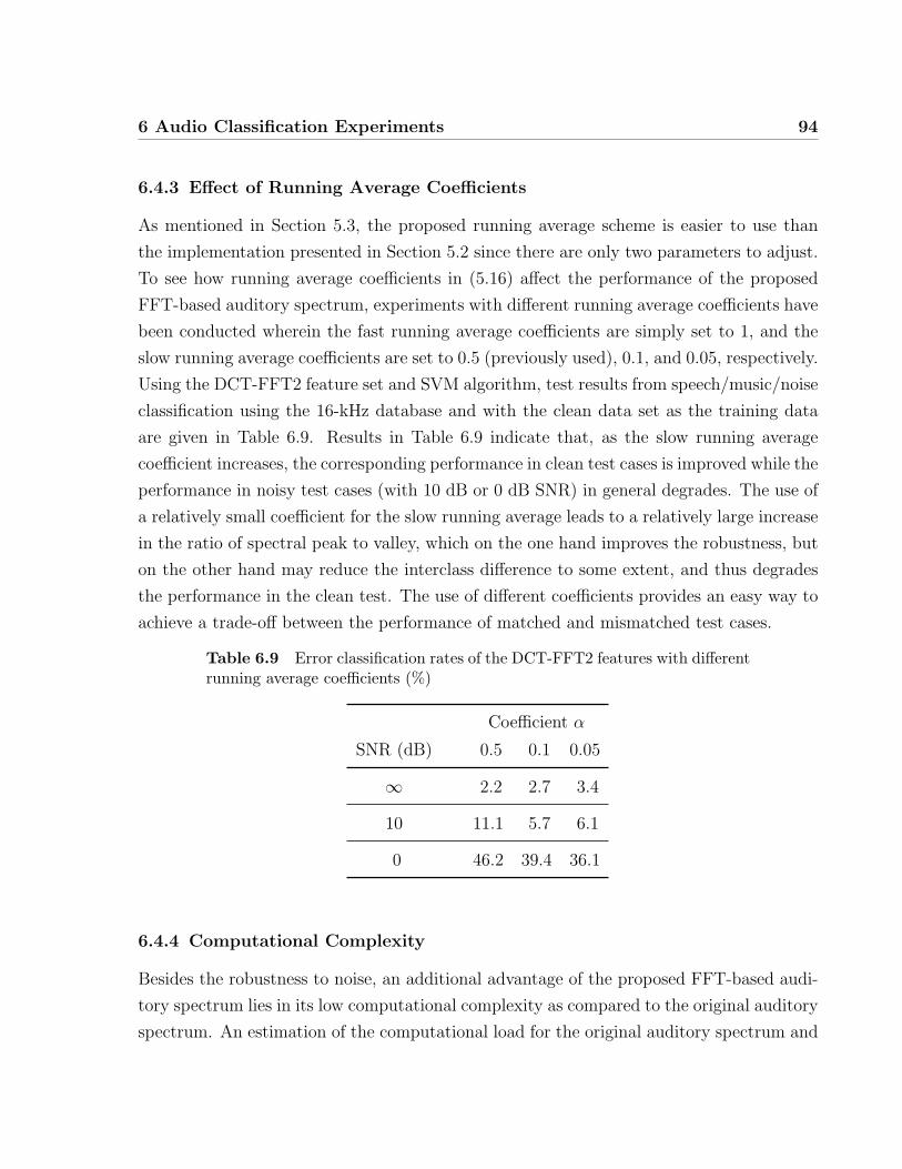
6 Audio Classification Experiments 94
6.4.3 Effect of Running Average Coefficients
As mentioned in Section 5.3, the proposed running average scheme is easier to use than
the implementation presented in Section 5.2 since there are only two parameters to adjust.
To see how running average coefficients in (5.16) affect the performance of the proposed
FFT-based auditory spectrum, experiments with different running average coefficients have
been conducted wherein the fast running average coefficients are simply set to 1, and the
slow running average coefficients are set to 0.5 (previously used), 0.1, and 0.05, respectively.
Using the DCT-FFT2 feature set and SVM algorithm, test results from speech/music/noise
classification using the 16-kHz database and with the clean data set as the training data
are given in Table 6.9. Results in Table 6.9 indicate that, as the slow running average
coefficient increases, the corresponding performance in clean test cases is improved while the
performance in noisy test cases (with 10 dB or 0 dB SNR) in general degrades. The use of
a relatively small coefficient for the slow running average leads to a relatively large increase
in the ratio of spectral peak to valley, which on the one hand improves the robustness, but
on the other hand may reduce the interclass difference to some extent, and thus degrades
the performance in the clean test. The use of different coefficients provides an easy way to
achieve a trade-off between the performance of matched and mismatched test cases.
Table 6.9 Error classification rates of the DCT-FFT2 features with differentrunning average coefficients (%)
Coefficient α
SNR (dB) 0.5 0.1 0.05
∞ 2.2 2.7 3.4
10 11.1 5.7 6.1
0 46.2 39.4 36.1
6.4.4 Computational Complexity
Besides the robustness to noise, an additional advantage of the proposed FFT-based audi-
tory spectrum lies in its low computational complexity as compared to the original auditory
spectrum. An estimation of the computational load for the original auditory spectrum and
6 Audio Classification Experiments 95
the proposed FFT-based auditory spectrum is obtained by measuring the corresponding
run time of the algorithm.
The implementation platform is a general PC with CPU Intel P4 (3.2 GHz). The
algorithms are implemented using Matlab. Results are obtained using the 16-kHz audio
database. Corresponding to a 1 s audio input clip, the time used for the calculation of
the original auditory spectrum and that of the proposed FFT-based auditory spectrum are
around 1.07 s and 0.08 s, respectively. Based on these results, compared to the original au-
ditory spectrum, the reduction in the processing time of the proposed FFT-based auditory
spectrum is more than a factor of 10. We will have more discussions on the complexity
issue of the proposed FFT-based auditory spectrum in the next chapter, wherein a DSP
implementation is conducted using a floating-point DSP platform.
6.5 Conclusion
In this Chapter, to evaluate the performance of the proposed FFT-based spectra, two audio
databases have been created with sampling rates of 16 and 8 kHz respectively. Three-class
(i.e., speech, music and noise) classification experiments have been conducted using the 16-
kHz database wherein SVM and C4.5 algorithms are used as the classifiers. Compared to
the conventional features, the auditory-related features (i.e., DCT-AUD, DCT-FFT1, DCT-
FFT2, and SPEC-FFT2) show more robust performance in mismatched test cases. Test
results also indicate that, using the DCT-based features, the performance of the proposed
FFT-based auditory spectrum is slightly better than that of the original auditory spectrum,
while the computational complexity is reduced by an order of magnitude. The robustness
of the DCT-based features computed from the proposed FFT-based auditory spectrum has
been further confirmed by test results of noise/non-noise classification experiments using
the 8-kHz database, and the effect of a running average coefficient was also investigated.
6 Audio Classification Experiments 96
97
Chapter 7
Implementation Based on
TMS320C6713 DSK
To further explore the proposed FFT-based auditory spectrum in the applications of audio
classification from a practical perspective, a three-class audio classification algorithm is
implemented on the floating-point TMS320C6713 DSP Starter Kit (DSK) [Spe04] from
Texas Instruments (TI), wherein the DCT-FFT2 features are extracted (see Section 6.2)
and the C4.5 decision tree model is used for the classification. A brief introduction to the
TMS320C6713 DSK1 is given in Appendix B.
In the presented DSP implementation, through a pair of input/output channels between
the host PC and DSP target board, audio data stored on the host PC are fed to the DSP
board as the input to the implemented classification algorithm, and the decisions of the
audio class are sent back to the host PC for the evaluation of the performance. The compu-
tational complexity of the proposed algorithm is investigated using TI’s real-time software
and development tool [Tex05a]. A significant reduction in the computational complex-
ity is achieved for the implemented algorithm through the use of different optimization
approaches.
1For the sake of simplicity, in this thesis, TMS320C67x and TMS320C6713 are sometimes simplified asC67x and C6713 respectively.
7 Implementation Based on TMS320C6713 DSK 98
7.1 Implementation of the Proposed Audio Classification
Algorithm
Using the C6713 DSK as the target, a three-class audio classification algorithm is imple-
mented below, wherein the DCT-based features calculated from the proposed FFT-based
auditory spectrum (i.e., DCT-FFT2 features, see Section 6.2) are used for the classification.
In the proposed implementation, to reduce the requirements on the memory units and the
computational complexity, we have used the relatively simple C4.5 decision tree model ob-
tained from the training phase as the classifier [Qui93]. The presented C6713 DSK-based
system demonstrates the ability to classify among speech, music and noise under constraints
of the real-time processing.
7.1.1 Structure of the System
We may divide the work of implementation into three parts, i.e., the classification algorithm,
the input/ouput scheme, and the monitoring of the output.
Audio Classification Algorithm
The audio classification decisions are made on a 1 s clip basis. This enables the algorithm to
wait until the data of a whole clip available in the buffer before the processing starts. In this
implementation, to reduce the requirements on the target’s memory units, the algorithm
is designed to work on a frame basis, which follows conventional ways of speech/audio
processing. Following this idea, the modules of the classification algorithm can be grouped
into two parts including the frame-based processing modules and the clip-based processing
modules.
Fig. 7.1 shows the modules of the algorithm. As discussed in Chapter 5, the calculation
of the proposed FFT-based auditory spectrum uses an analysis window of 30 ms with
an overlap of 20 ms. Therefore, for each frame of 10 ms input signal, the frame-based
processing operations output a set of frame-level DCT-FFT2 features.
The clip-level processing is triggered as soon as all signal frames in a clip have been
processed. Therefore, the computational load of the last frame in a clip will be in general
higher than any other frames in the same clip since both frame-level and clip-level operations
are involved.
7 Implementation Based on TMS320C6713 DSK 99
For an ANSI (American National Standards Institute) C algorithm, all these modules
can be simply integrated in the main function to get the desired output. However, for
a C6713 DSK-based implementation, this needs to be modified due to the use of the in-
put/output scheme as described later. Specifically, we now have two functions, namely:
main and classify. The processing modules shown in Fig. 7.1 are placed in the function
classify which is acted as an interrupt service routine (ISR) and is triggered under certain
conditions as specified by the configurations of the input/output scheme and the software
interrupt objects. For function main, it is now used only to facilitate the input/output
transmission supported by DSP/BIOS. We will have more discussions on this given below.
Input/Output with Host Channel
Two host channels provided by the C6713 DSK are used in this work to implement the
input and output channels between the host PC and the DSP target for the proposed audio
classification implementation.
Host channel objects are managed by the DSP/BIOS’s HST module [Tex04b, Tex04c].
Host channel objects provide a run-time communication link between the host and the
target. When using HST module, the host PC reads or writes data using LNK dataPump
object, which is a built-in IDL object that runs its function as part of the background
threads [Tex04b, Tex04c]. Since background threads have the lowest priority, on the C6000
platforms, the actual data transfer occurs at high priority by triggering interrupts.
Each host channel is internally implemented using a data pipe object, which is managed
by the PIP module [Tex04b, Tex04c]. Pipes are designed to manage block input/output
(also called stream-based or asynchronous input/output). Each pipe object maintains
a buffer divided into a fixed number of frames, with each frame a fixed length. The
input/output operations on a pipe deal with one frame at a time. As shown in Fig. 7.2,
a pipe has two ends, the writer and the reader. The writer end (also called producer) is
where a program writes frames of data, whereas the reader end (also called consumer) is
where a program reads frames of data. Two data notification functions, notifyReader and
notifyWriter, are employed to synchronize the data transfer.
When a frame of data is written into the pipe, the writer end calls PIP put function to
put the frame into the pipe. The function notifyReader is triggered to notify the program
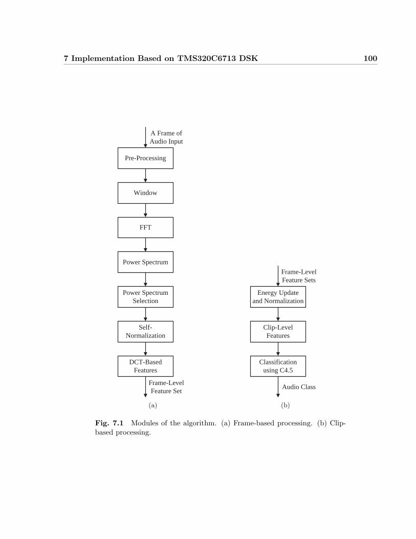
7 Implementation Based on TMS320C6713 DSK 100
FFT
Window
A Frame of Audio Input
Pre-Processing
Power Spectrum
Power Spectrum Selection
Self- Normalization
DCT-Based Features
Frame-Level Feature Set
(a)
Clip-Level Features
Frame-Level Feature Sets
Energy Update and Normalization
Classification using C4.5
Audio Class
(b)
Fig. 7.1 Modules of the algorithm. (a) Frame-based processing. (b) Clip-based processing.
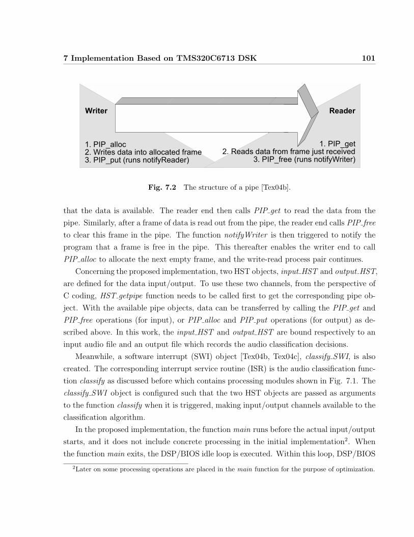
7 Implementation Based on TMS320C6713 DSK 101
PIP Module
2-208
Figure 2-2. Pipe Schematic
Internally, pipes are implemented as a circular list; frames are reused atthe writer end of the pipe after PIP_free releases them.
The notifyReader and notifyWriter functions are called from the contextof the code that calls PIP_put or PIP_free. These functions can be writtenin C or assembly. To avoid problems with recursion, the notifyReader andnotifyWriter functions normally should not directly call any of the PIPmodule functions for the same pipe. Instead, they should post a softwareinterrupt that uses the PIP module functions. However, PIP calls may bemade from the notifyReader and notifyWriter functions if the functionshave been protected against re-entrancy. The audio example, located onyour distribution CD in c:\ti\examples\target\bios\audio folder,where target matches your board, is a good example of this. (If youinstalled in a path other than c:\ti, substitute your appropriate path.)
ReaderWriter
1. PIP_alloc2. Writes data into allocated frame3. PIP_put (runs notifyReader)
1. PIP_get2. Reads data from frame just received
3. PIP_free (runs notifyWriter)
Fig. 7.2 The structure of a pipe [Tex04b].
that the data is available. The reader end then calls PIP get to read the data from the
pipe. Similarly, after a frame of data is read out from the pipe, the reader end calls PIP free
to clear this frame in the pipe. The function notifyWriter is then triggered to notify the
program that a frame is free in the pipe. This thereafter enables the writer end to call
PIP alloc to allocate the next empty frame, and the write-read process pair continues.
Concerning the proposed implementation, two HST objects, input HST and output HST,
are defined for the data input/output. To use these two channels, from the perspective of
C coding, HST getpipe function needs to be called first to get the corresponding pipe ob-
ject. With the available pipe objects, data can be transferred by calling the PIP get and
PIP free operations (for input), or PIP alloc and PIP put operations (for output) as de-
scribed above. In this work, the input HST and output HST are bound respectively to an
input audio file and an output file which records the audio classification decisions.
Meanwhile, a software interrupt (SWI) object [Tex04b, Tex04c], classify SWI, is also
created. The corresponding interrupt service routine (ISR) is the audio classification func-
tion classify as discussed before which contains processing modules shown in Fig. 7.1. The
classify SWI object is configured such that the two HST objects are passed as arguments
to the function classify when it is triggered, making input/output channels available to the
classification algorithm.
In the proposed implementation, the function main runs before the actual input/output
starts, and it does not include concrete processing in the initial implementation2. When
the function main exits, the DSP/BIOS idle loop is executed. Within this loop, DSP/BIOS
2Later on some processing operations are placed in the main function for the purpose of optimization.
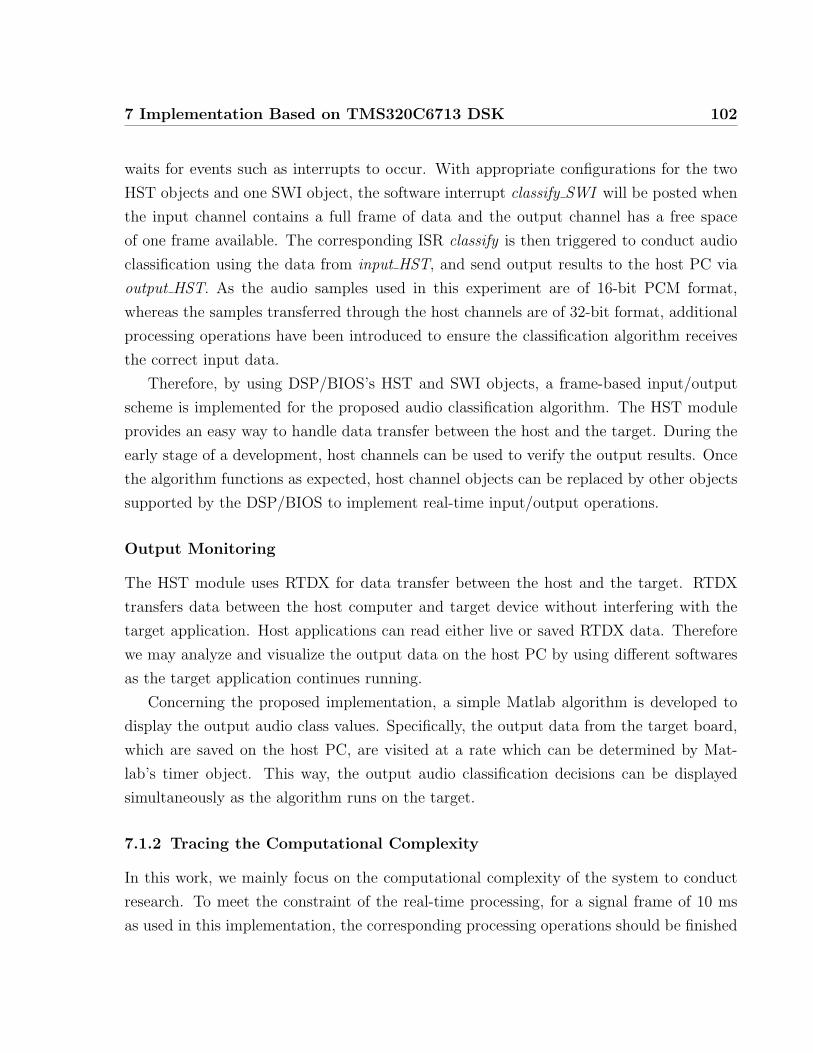
7 Implementation Based on TMS320C6713 DSK 102
waits for events such as interrupts to occur. With appropriate configurations for the two
HST objects and one SWI object, the software interrupt classify SWI will be posted when
the input channel contains a full frame of data and the output channel has a free space
of one frame available. The corresponding ISR classify is then triggered to conduct audio
classification using the data from input HST, and send output results to the host PC via
output HST. As the audio samples used in this experiment are of 16-bit PCM format,
whereas the samples transferred through the host channels are of 32-bit format, additional
processing operations have been introduced to ensure the classification algorithm receives
the correct input data.
Therefore, by using DSP/BIOS’s HST and SWI objects, a frame-based input/output
scheme is implemented for the proposed audio classification algorithm. The HST module
provides an easy way to handle data transfer between the host and the target. During the
early stage of a development, host channels can be used to verify the output results. Once
the algorithm functions as expected, host channel objects can be replaced by other objects
supported by the DSP/BIOS to implement real-time input/output operations.
Output Monitoring
The HST module uses RTDX for data transfer between the host and the target. RTDX
transfers data between the host computer and target device without interfering with the
target application. Host applications can read either live or saved RTDX data. Therefore
we may analyze and visualize the output data on the host PC by using different softwares
as the target application continues running.
Concerning the proposed implementation, a simple Matlab algorithm is developed to
display the output audio class values. Specifically, the output data from the target board,
which are saved on the host PC, are visited at a rate which can be determined by Mat-
lab’s timer object. This way, the output audio classification decisions can be displayed
simultaneously as the algorithm runs on the target.
7.1.2 Tracing the Computational Complexity
In this work, we mainly focus on the computational complexity of the system to conduct
research. To meet the constraint of the real-time processing, for a signal frame of 10 ms
as used in this implementation, the corresponding processing operations should be finished
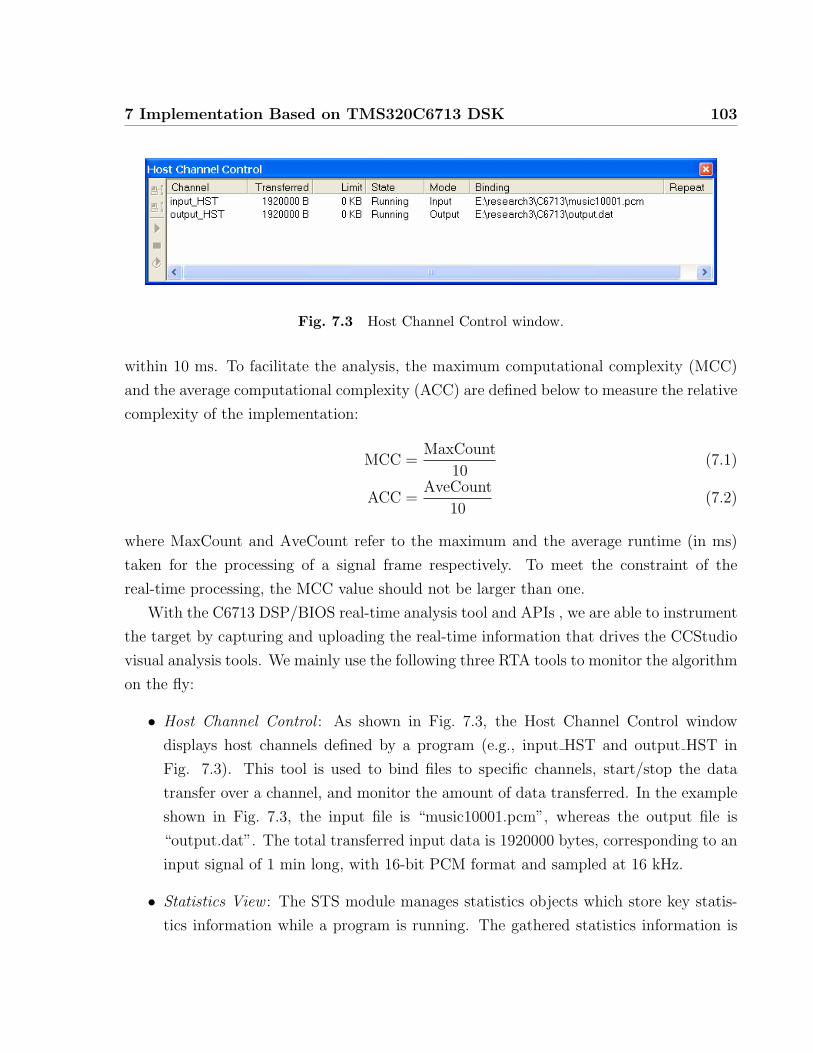
7 Implementation Based on TMS320C6713 DSK 103
Fig. 7.3 Host Channel Control window.
within 10 ms. To facilitate the analysis, the maximum computational complexity (MCC)
and the average computational complexity (ACC) are defined below to measure the relative
complexity of the implementation:
MCC =MaxCount
10(7.1)
ACC =AveCount
10(7.2)
where MaxCount and AveCount refer to the maximum and the average runtime (in ms)
taken for the processing of a signal frame respectively. To meet the constraint of the
real-time processing, the MCC value should not be larger than one.
With the C6713 DSP/BIOS real-time analysis tool and APIs , we are able to instrument
the target by capturing and uploading the real-time information that drives the CCStudio
visual analysis tools. We mainly use the following three RTA tools to monitor the algorithm
on the fly:
• Host Channel Control : As shown in Fig. 7.3, the Host Channel Control window
displays host channels defined by a program (e.g., input HST and output HST in
Fig. 7.3). This tool is used to bind files to specific channels, start/stop the data
transfer over a channel, and monitor the amount of data transferred. In the example
shown in Fig. 7.3, the input file is “music10001.pcm”, whereas the output file is
“output.dat”. The total transferred input data is 1920000 bytes, corresponding to an
input signal of 1 min long, with 16-bit PCM format and sampled at 16 kHz.
• Statistics View : The STS module manages statistics objects which store key statis-
tics information while a program is running. The gathered statistics information is
7 Implementation Based on TMS320C6713 DSK 104
Fig. 7.4 Statistics View window.
presented in Statistics View window, as shown in Fig. 7.4. In this window, “Count”
reports the number of times a thread or a code segment executed. The instructions
or the runtime used for the execution of a thread or a code segment are also reported,
with “Total”, “Max”, and “Average” representing the corresponding arithmetic sum,
the maximum value, and the average value, respectively.
Statistics about the SWI (software interrupt), PRD (period), HWI (hardware in-
terrupt), PIP (pipe), and TSK (task) objects are captured automatically. This is
called the implicit instrumentation. For example, in Fig. 7.4, the statistics infor-
mation shown in the first line denotes the execution of a software interrupt called
“classify SWI”. Besides the implicit instrumentation, explicit instrumentation can be
used to accumulate statistics explicitly through DSP/BIOS API calls. For example,
we may track statistics such as the amount of time it takes to perform a section of
code as follows:
STS set(&stsObj, CLK gethtime());
......(the segment of the code under test)
STS delta(&stsObj,CLK gethtime());
Here, STS set saves a high-resolution time value, which is returned by the function
CLK gethtime, as the initial value in an STS object. STS delta subtracts this saved
initial value from a new value returned by another CLK gethtime. The second line in
the Statistics View window in Fig. 7.4 is an example of such explicit instrumentation
wherein a statistics object called “STS2” is defined to benchmark a specific part of
the code.
Both the implicit and explicit instrumentations are used in our experiment to gather
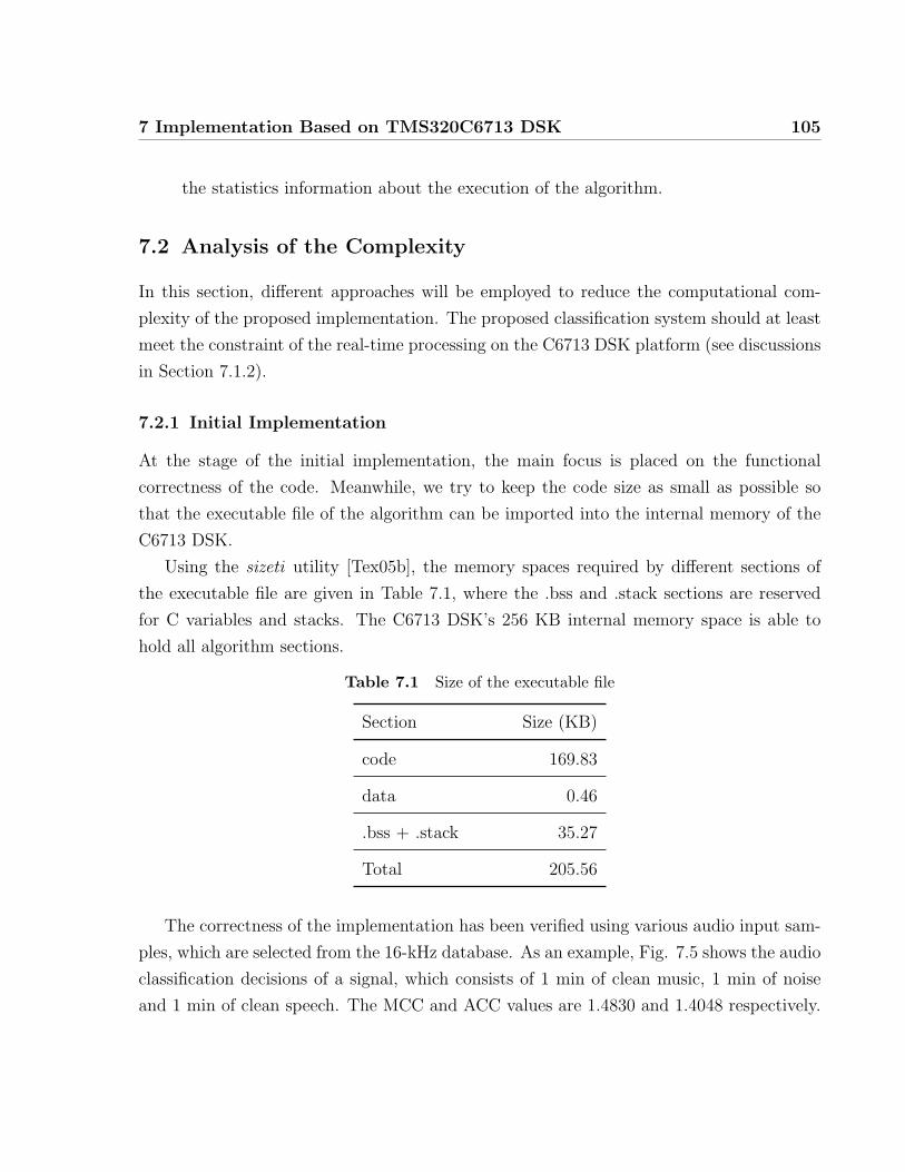
7 Implementation Based on TMS320C6713 DSK 105
the statistics information about the execution of the algorithm.
7.2 Analysis of the Complexity
In this section, different approaches will be employed to reduce the computational com-
plexity of the proposed implementation. The proposed classification system should at least
meet the constraint of the real-time processing on the C6713 DSK platform (see discussions
in Section 7.1.2).
7.2.1 Initial Implementation
At the stage of the initial implementation, the main focus is placed on the functional
correctness of the code. Meanwhile, we try to keep the code size as small as possible so
that the executable file of the algorithm can be imported into the internal memory of the
C6713 DSK.
Using the sizeti utility [Tex05b], the memory spaces required by different sections of
the executable file are given in Table 7.1, where the .bss and .stack sections are reserved
for C variables and stacks. The C6713 DSK’s 256 KB internal memory space is able to
hold all algorithm sections.
Table 7.1 Size of the executable file
Section Size (KB)
code 169.83
data 0.46
.bss + .stack 35.27
Total 205.56
The correctness of the implementation has been verified using various audio input sam-
ples, which are selected from the 16-kHz database. As an example, Fig. 7.5 shows the audio
classification decisions of a signal, which consists of 1 min of clean music, 1 min of noise
and 1 min of clean speech. The MCC and ACC values are 1.4830 and 1.4048 respectively.
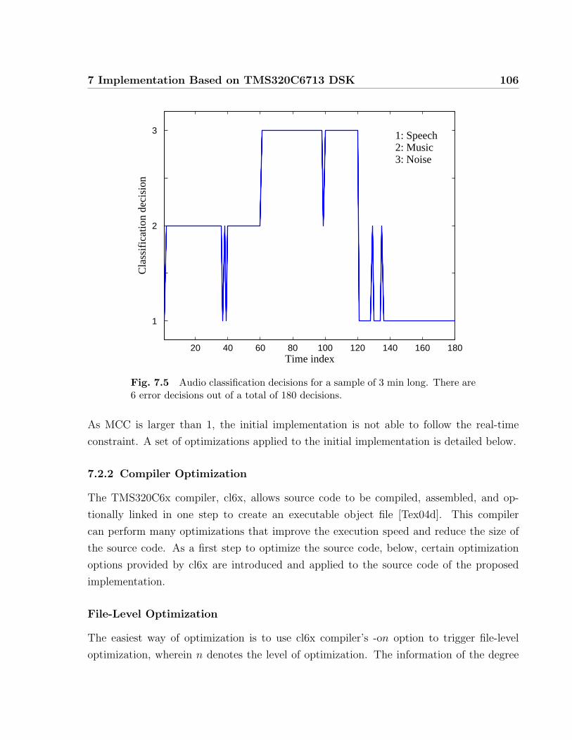
7 Implementation Based on TMS320C6713 DSK 106
20 40 60 80 100 120 140 160 180
1
2
3
Time index
Cla
ssif
icat
ion
deci
sion
1: Speech2: Music3: Noise
Fig. 7.5 Audio classification decisions for a sample of 3 min long. There are6 error decisions out of a total of 180 decisions.
As MCC is larger than 1, the initial implementation is not able to follow the real-time
constraint. A set of optimizations applied to the initial implementation is detailed below.
7.2.2 Compiler Optimization
The TMS320C6x compiler, cl6x, allows source code to be compiled, assembled, and op-
tionally linked in one step to create an executable object file [Tex04d]. This compiler
can perform many optimizations that improve the execution speed and reduce the size of
the source code. As a first step to optimize the source code, below, certain optimization
options provided by cl6x are introduced and applied to the source code of the proposed
implementation.
File-Level Optimization
The easiest way of optimization is to use cl6x compiler’s -on option to trigger file-level
optimization, wherein n denotes the level of optimization. The information of the degree
7 Implementation Based on TMS320C6713 DSK 107
of optimization is summarized below [Tex04d]:
• -o0
Performs control-flow-graph simplification; allocates variables to registers; performs
loop rotation; eliminates unused code; simplifies expressions and statements; and
expands calls to functions declared inline.
• -o1
Performs all -o0 optimizations; performs local copy/constant propagation; removes
unused assignments; eliminates local common expressions.
• -o2
Performs all -o1 optimizations; performs software pipelining; performs loop optimiza-
tions; eliminates global common subexpressions; eliminates global unused assign-
ments; converts array references in loops to incremented pointer form; and performs
loop unrolling.
• -o3
Performs all -o2 optimizations; removes all functions that are never called; simplifies
functions with return values that are never used; inlines calls to small functions;
reorders function declarations so that the attributes of called functions are known
when the caller is optimized; propagates arguments into function bodies when all
calls pass the same value in the same argument position; and identifies file-level
variable characteristics.
Option -o3 is used below for file-level optimization.
Program-Level Optimization
For multiple source files, program-level optimization can be specified by using -pm option
together with -o3 option. With program-level optimization, all source files are compiled
into one intermediate file called a module. With program-level optimization, the compiler
can “see” the entire program, and then perform several optimizations that are beyond the
scope of a file-level optimization. The optimization operations may include:
• If a particular argument in a function always has the same value, the compiler replaces
the argument with the value and passes the value instead of the argument.
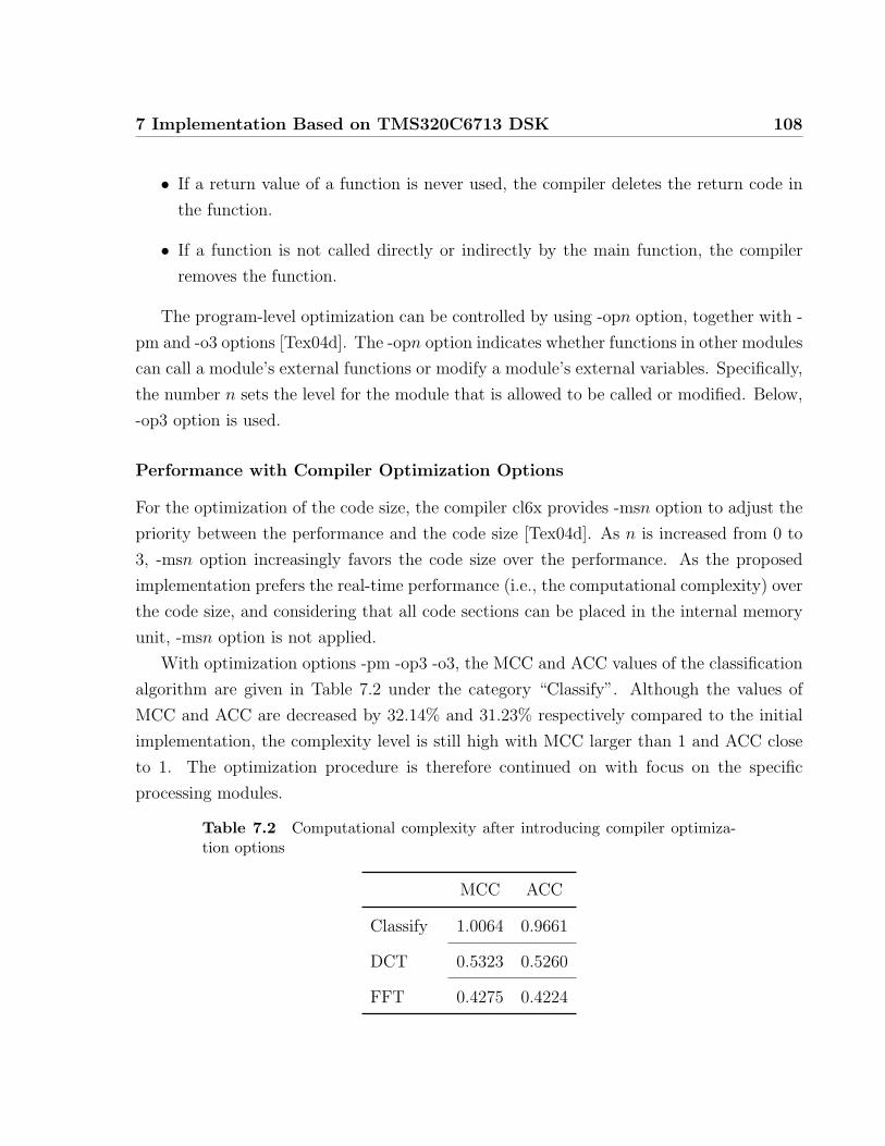
7 Implementation Based on TMS320C6713 DSK 108
• If a return value of a function is never used, the compiler deletes the return code in
the function.
• If a function is not called directly or indirectly by the main function, the compiler
removes the function.
The program-level optimization can be controlled by using -opn option, together with -
pm and -o3 options [Tex04d]. The -opn option indicates whether functions in other modules
can call a module’s external functions or modify a module’s external variables. Specifically,
the number n sets the level for the module that is allowed to be called or modified. Below,
-op3 option is used.
Performance with Compiler Optimization Options
For the optimization of the code size, the compiler cl6x provides -msn option to adjust the
priority between the performance and the code size [Tex04d]. As n is increased from 0 to
3, -msn option increasingly favors the code size over the performance. As the proposed
implementation prefers the real-time performance (i.e., the computational complexity) over
the code size, and considering that all code sections can be placed in the internal memory
unit, -msn option is not applied.
With optimization options -pm -op3 -o3, the MCC and ACC values of the classification
algorithm are given in Table 7.2 under the category “Classify”. Although the values of
MCC and ACC are decreased by 32.14% and 31.23% respectively compared to the initial
implementation, the complexity level is still high with MCC larger than 1 and ACC close
to 1. The optimization procedure is therefore continued on with focus on the specific
processing modules.
Table 7.2 Computational complexity after introducing compiler optimiza-tion options
MCC ACC
Classify 1.0064 0.9661
DCT 0.5323 0.5260
FFT 0.4275 0.4224
7 Implementation Based on TMS320C6713 DSK 109
By using explicit instrumentations, the two modules with the heaviest computational
loads are further identified, and their complexity values are also presented in Table 7.2 under
categories “DCT” and “FFT”, corresponding to the calculation of DCT-based features and
the computation of 1024-point FFT, respectively. Taking MCC for example, more than 95%
of the total computational complexity is due to these two modules. Below, optimization
approaches are introduced to lower the complexity levels for these two modules.
7.2.3 Optimization of DCT and FFT Modules
Use of a Coefficient Table for DCT Module
Through an investigation into the DCT module, its heavy computational load comes in a
large part from the calculation of cosine coefficients (refer to (6.2)). As these coefficients
are unchanged throughout the processing, we can tabulate these coefficients instead of
calculating them each time they are used. Considering this, the module is re-organized into
two submodules, wherein the first submodule contains the calculation of cosine coefficients,
whereas the second submodule conducts the calculation of the DCT-based features using
the cosine coefficients prepared by the first submodule.
As the first submodule only needs to run once throughout the processing, it is now
placed in the function main and acts as the initial processing of the whole algorithm. The
second submodule is left in the function classify (the interrupt service routine) to replace
the original DCT module. Therefore, before the actual audio input/output begins, these
cosine coefficients are available for the calculation of the DCT-based features. The real-
time computational complexity is now determined only by the second submodule wherein
a significant reduction in the computational complexity can be achieved as expected. The
detailed information on the reduction in the complexity is reported later.
Use of C67x Optimized DSP Library Functions for the FFT Module
For the FFT module, the initial implementation employs a radix-2 decimation in time
(DIT) algorithm [OSB99]. Similarly, there are lots of cosine and sine functions involved
in the calculation of the FFT due to the coefficients W kN = e−j2πk/N . We may use a
same approach as described above to calculate the coefficients W kN separately to reduce the
computational complexity. An existing optimized FFT function DSPF sp cfftr2 dit, which
takes this same idea to calculate FFT, is available from TI’s C67x optimized DSP Library
7 Implementation Based on TMS320C6713 DSK 110
(DSPLIB) [Tex06]. This optimized function is now used to replace the FFT algorithm in
the initial implementation.
The C67x DSPLIB is an optimized DSP function library, which includes C-callable,
assembly-optimized, general-purpose signal processing routines. DSPLIB provides routines
in both single and double precisions. These functions cover the processing or computa-
tion of adaptive filtering, correlation, FFT, filtering and convolution, matrix operation,
etc. DSPLIB can be used in computationally intensive real-time applications to achieve
execution speeds considerably faster than the equivalent code written in standard ANSI C
language.
The C-callable optimized FFT function used in this work is DSPF sp cfftr2 dit, which
is a single-precision floating-point radix-2 DIT FFT algorithm for complex input. The
function is declared as follows:
void DSPF sp cfftr2 dit(float *x, float *w, short n) (7.3)
where argument x contains n = N complex input/output numbers arranged as successive
real and imaginary pairs (i.e., 2N elements in total), w contains N/2 complex coefficients
W kN arranged as successive real and imaginary pairs, and n = N is the length of the FFT in
complex samples and it must be a power of 2 and greater than or equal to 32. The elements
of the input array x are in normal order, whereas the outputs in x are in bit-reversed order.
The coefficients w are in bit-reversed order. The complete steps of the FFT calculation
using the optimized function DSPF sp cfftr2 dit are summarized below [Tex06]:
Step 1: Generate coefficient table w using C function gen twiddle(w,N)
Step 2: Bit-reverse coefficient table w using C function bit rev(w,N/2)
Step 3: Conduct FFT using assembly-optimized function DSPF sp cfftr2 dit(x,w,N)
Step 4: Bit-reverse output x using C function bit rev(x,N)
Clearly, the calculation of the coefficient table w (Steps 1 and 2) can be placed in the initial
processing of the algorithm in the function main. Therefore, only the calculations involved
in Steps 3 and 4 contribute to the real-time computational complexity. In addition, the
C67x DSPLIB provides another optimized function, DSPF sp bitrev cplx, to bit-reverse
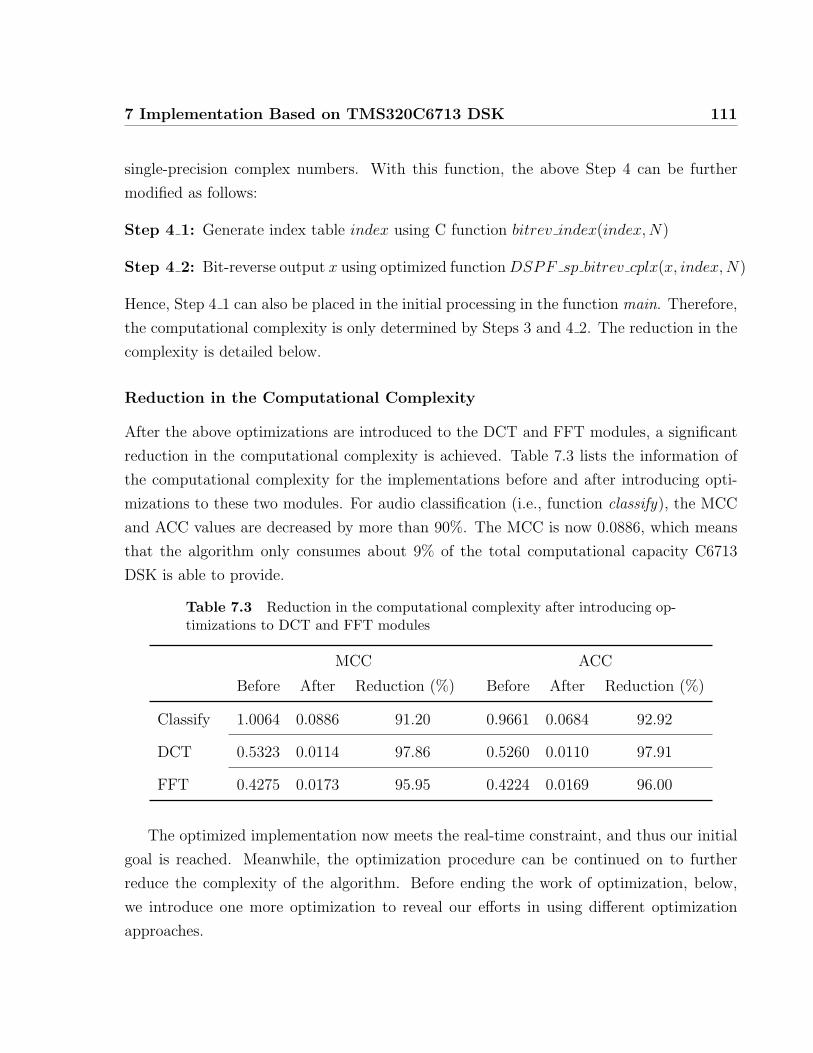
7 Implementation Based on TMS320C6713 DSK 111
single-precision complex numbers. With this function, the above Step 4 can be further
modified as follows:
Step 4 1: Generate index table index using C function bitrev index(index,N)
Step 4 2: Bit-reverse output x using optimized functionDSPF sp bitrev cplx(x, index,N)
Hence, Step 4 1 can also be placed in the initial processing in the function main. Therefore,
the computational complexity is only determined by Steps 3 and 4 2. The reduction in the
complexity is detailed below.
Reduction in the Computational Complexity
After the above optimizations are introduced to the DCT and FFT modules, a significant
reduction in the computational complexity is achieved. Table 7.3 lists the information of
the computational complexity for the implementations before and after introducing opti-
mizations to these two modules. For audio classification (i.e., function classify), the MCC
and ACC values are decreased by more than 90%. The MCC is now 0.0886, which means
that the algorithm only consumes about 9% of the total computational capacity C6713
DSK is able to provide.
Table 7.3 Reduction in the computational complexity after introducing op-timizations to DCT and FFT modules
MCC ACC
Before After Reduction (%) Before After Reduction (%)
Classify 1.0064 0.0886 91.20 0.9661 0.0684 92.92
DCT 0.5323 0.0114 97.86 0.5260 0.0110 97.91
FFT 0.4275 0.0173 95.95 0.4224 0.0169 96.00
The optimized implementation now meets the real-time constraint, and thus our initial
goal is reached. Meanwhile, the optimization procedure can be continued on to further
reduce the complexity of the algorithm. Before ending the work of optimization, below,
we introduce one more optimization to reveal our efforts in using different optimization
approaches.
7 Implementation Based on TMS320C6713 DSK 112
7.2.4 Use of C67x FastRTS Optimized Library
After introducing optimizations to the DCT and FFT modules, it is found that the spectral
self-normalization module (see Fig. 7.1) is now the most critical part wherein about 40.45%
of the total computational complexity (based on the MCC value) is due to this module. The
calculations involved in the spectral self-normalization module follow the ideas described in
Section 5.3.4, wherein the relatively high complexity level is due to the division and square-
root operations in a loop. To conduct optimization for these two operations, we may use
C67x’s assembly-optimized division and square-root subroutines, which are included in the
C67x fast run-time-support (FastRTS) library [Tex02].
C67x FastRTS library is an optimized floating-point math function library for program-
mers using TMS320C67x devices. This library provides hand-coded assembly-optimized
routines that are C-callable for some computational intensive functions, such as sine, co-
sine, logarithm, exponential, reciprocal, etc. A considerably faster execution speed can be
achieved through testings against C model and existing run-time-support functions [Tex02].
Concerning the proposed implementation, single-precision floating-point functions divsp
and sqrtf provided by the C67x FastRTS library are used to replace the corresponding
existing division and square-root operations in the self-normalization module. Since the
FastRTS library is a subset of the standard RTS library, if we want to use FastRTS library
functions in place of the existing versions of these functions, the FastRTS library must be
linked in before the existing RTS library [Tex02].
The reduction in the computational complexity is achieved and verified by testing results
given in Table 7.4, where “Self-Norm” refers to the spectral self-normalization module. It
is also found that by using the FastRTS library, additional reductions in the computational
complexity are achieved for some other modules. The reason is that some FastRTS library
functions have replaced the existing functions as mentioned before. According to Table 7.4,
the MCC and ACC values of the classification algorithm are further reduced by 39.62%
and 46.49% respectively. The information of the code size is listed in Table 7.5. After all
above optimization approaches have been introduced, the code size is increased by about
12 kB compared to the data given in Table 7.1. This increase in the code size is not critical
as the internal memory space of 256 kB is still large enough to place the executable file of
the algorithm.
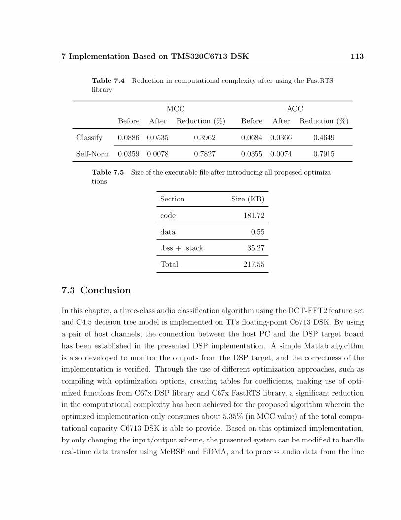
7 Implementation Based on TMS320C6713 DSK 113
Table 7.4 Reduction in computational complexity after using the FastRTSlibrary
MCC ACC
Before After Reduction (%) Before After Reduction (%)
Classify 0.0886 0.0535 0.3962 0.0684 0.0366 0.4649
Self-Norm 0.0359 0.0078 0.7827 0.0355 0.0074 0.7915
Table 7.5 Size of the executable file after introducing all proposed optimiza-tions
Section Size (KB)
code 181.72
data 0.55
.bss + .stack 35.27
Total 217.55
7.3 Conclusion
In this chapter, a three-class audio classification algorithm using the DCT-FFT2 feature set
and C4.5 decision tree model is implemented on TI’s floating-point C6713 DSK. By using
a pair of host channels, the connection between the host PC and the DSP target board
has been established in the presented DSP implementation. A simple Matlab algorithm
is also developed to monitor the outputs from the DSP target, and the correctness of the
implementation is verified. Through the use of different optimization approaches, such as
compiling with optimization options, creating tables for coefficients, making use of opti-
mized functions from C67x DSP library and C67x FastRTS library, a significant reduction
in the computational complexity has been achieved for the proposed algorithm wherein the
optimized implementation only consumes about 5.35% (in MCC value) of the total compu-
tational capacity C6713 DSK is able to provide. Based on this optimized implementation,
by only changing the input/output scheme, the presented system can be modified to handle
real-time data transfer using McBSP and EDMA, and to process audio data from the line
7 Implementation Based on TMS320C6713 DSK 114
input on the AIC23 codec and plays the result on the line output [Spe04].

7 Implementation Based on TMS320C6713 DSK 115
116
Chapter 8
Summary and Conclusion
8.1 Summary of the Work
The past decade has seen extensive research on the content-based audio analysis. Current
research interests lie in the classification/segmentation, the information retrieval, and the
indexing. Among these applications, audio classification is the fundamental process which
can be employed as a basis for other applications. The scope of this work is focused on
audio classification algorithms.
Various audio classification algorithms have been proposed along with excellent perfor-
mance being reported. Among different audio classes, speech and music are the two most
popular classes in multimedia communications, and thus have attracted much attention in
audio classification applications. Such speech/music classification algorithms can be used
for different purposes, e.g., to surf a radio channel for segments of music or talk. Besides
speech and music, some researchers have included other audio classes in their studies, es-
pecially various environmental sounds and background noises, due to considerations on
certain practical applications wherein the background sounds or noises are present.
The design of audio features is a key issue in the development of an audio classification
algorithm. A good feature characterizes a large interclass difference and a small intraclass
difference. Audio features are commonly extracted in two levels, namely: the short-term
frame level and the long-term clip level. The frame-level features are usually calculated
through time-domain analysis, Fourier transform analysis, LPC analysis, etc. Widely used
frame-level features include the short-time energy, the short-time average ZCR, the pitch
frequency, the spectral centroid, the MFCCs, the LPC coefficients, etc. Clip-level features
8 Summary and Conclusion 117
usually describe how frame-level features change over a time window. The most widely used
clip-level features are the statistical mean and variance values of the frame-level features
such as the energy and ZCR.
Various classification approaches have been employed in audio classification applica-
tions. For an application where there is requirements for low complexity and real-time
processing, the simple rule-based classifiers are appropriate. Other relatively complex pat-
tern recognition approaches commonly used in audio classification applications include the
HMM, the SVM, the GMM, etc.
Although in some audio classification applications the presence of background noise has
been considered, such considerations are limited to using background noise as one of the
audio classes or as a component of some hybrid sounds. The effect of background noise on
the performance of classification has not been widely investigated. In fact, a classification
algorithm trained using clean sequences may fail to work properly when the actual testing
sequences contain background noise with certain SNR levels. The so-called early auditory
model presented by Wang and Shamma [WS94] is proved to be robust in noisy environments
due to an inherent self-normalization property which causes noise suppression. Recently,
this model has been employed in audio classification experiments in [RA04] and noise-robust
performance has been reported.
Noise-robustness is a property that is lacking in many of today’s audio classification
and speech recognition systems. Inspired by the noise-suppression property of the EA
model [WS94], we seek in this thesis to further explore the application of this property to
audio classification algorithms. A series of related research work has been conducted which
forms the basis of the proposed study on auditory-inspired noise-robust audio classification
algorithms. The proposed research has led to main achievements as summarized below.
First, we have used the Gaussian CDF as an approximation to the original sigmoid
compression function to derive a new closed-form expression for the auditory spectrum (i.e.,
the output of the EA model) and to conduct relevant analysis. The use of the Gaussian CDF
is based on its nonlinear compression nature, and its resemblance to the sigmoid function.
The new results based on the Gaussian CDF verify the self-normalization property as
analyzed in [WS94]. Compared to the original analysis wherein a step function is used to
approximate the nonlinear sigmoid compression function, the proposed analysis using the
Gaussian CDF provides a better yet mathematically tractable approximation.
Second, efforts have been made to propose simplified and approximated versions of
8 Summary and Conclusion 118
the original auditory spectrum. Based on the original time-domain analysis in [WS94], a
simplified auditory spectrum has been proposed, which provides a way to investigate the
approximation of the EA model from the perspective of linear processing. The under-
lying analysis naturally leads to frequency-domain approaches for further approximation
in order to achieve a significant reduction in the computational complexity. A simplified
FFT-based spectrum is then proposed wherein a local spectral self-normalization is im-
plemented through the use of a pair of wide and narrow filters defined in the frequency
domain. Furthermore, an improved implementation of the above FFT-based spectrum is
proposed to calculate a so-called simplified FFT-based auditory spectrum. The introduced
improvements include the use of characteristic frequency (CF) values of the cochlear filters
in the original EA model for the power spectrum selection, and the use of a pair of fast and
slow running averages over the frequency axis to implement the spectral self-normalization.
With the introduced improvements, the proposed FFT-based auditory spectrum allows
more flexibility in the extraction of noise-robust audio features.
Third, to evaluate the performance of the proposed FFT-based spectrum (see Section
5.2) and the proposed FFT-based auditory spectrum (see Section 5.3), audio classification
experiments have been carried out. Two generic audio databases were created which con-
tain speech, music and noise clips. The sampling rates of the two databases are 16 and 8
kHz. The DCT-based frame-level audio features were calculated using the original audi-
tory spectrum, the proposed FFT-based spectrum, and the proposed FFT-based auditory
spectrum. In addition, frame-level audio features also include a set of spectral features cal-
culated using the proposed FFT-based auditory spectrum. The clip-level features used in
this study are simply the statistical mean and variance values of the corresponding frame-
level features. As for the classification approach, we have used the SVMstruct algorithm
[TJHA05]) and the C4.5 algorithm [Qui93]. The experimental platforms include Matlab
and ANSI C. Three-class (i.e., speech, music and noise) and two-class (noise and non-noise)
classification experiments have been conducted to evaluate the classification performance.
Specifically, mismatched tests are conducted to evaluate the noise-robustness of various
features, wherein the training and testing sets contain samples with mismatched SNR val-
ues. Compared to the conventional features such as MFCCs, the auditory-related features
(i.e., features obtained from the original auditory spectrum and the proposed FFT-based
spectra) show more robust performance in mismatched test cases. Test results also indicate
that the performance of the proposed FFT-based auditory spectrum is slightly better than
8 Summary and Conclusion 119
that of the original auditory spectrum, while its computational complexity is reduced by
an order of magnitude.
Finally, to further explore the proposed FFT-based auditory spectrum from a practical
perspective, a three-class audio classification algorithm has been developed and tested
on the TI’s floating-point DSP platform TMS320C6713 DSK. The algorithm employs the
DCT-based feature set (i.e., DCT-FFT2 feature set) and the C4.5 decision tree model.
Through the use a pair of host channels, the connection between the host PC and the DSP
target has been established in the presented implementation. The input audio signals are
16-bit signed PCM data which are sampled at 16 kHz and stored on the host PC, whereas
the outputs of the system are audio classification decisions on a 1 s basis. A simple Matlab
algorithm is also developed to monitor the outputs from the DSP target. By using TI’s
real-time software development tool, we have investigated the computational complexity
of the algorithm. Through different optimization approaches, such as the use of tools and
optimized functions provided by the C6713 DSK, we have achieved a significant reduction
in the computational complexity for the proposed implementation.
8.2 Future Research
The proposed research may be further explored from the following perspectives:
• Spectral enhancement along the time index : The proposed self-normalization is im-
plemented in the FFT-domain by using a pair of wide and narrow filters defined over
the frequency channel index. For audio classification applications, as introduced ear-
lier, some clip-level features are designed to characterize the temporal variation of
frame-level features. As such, enhancement along the time index may also lead to the
desired noise suppression. Specifically, it is of interest to investigate if a channel-time
(or space-time) joint spectral enhancement approach can be developed to calculate
some noise-robust FFT-based spectrogram, from which we may achieve further im-
provement in the noise suppression with application in audio classification.
• Experimental setup: The noise-robustness of the proposed approaches has been eval-
uated in audio classification experiments described in Chapter 6. Regarding the
classifiers and the audio features used in this work, we may change to use some other
8 Summary and Conclusion 120
classification approaches and to calculate other audio features so as to further evaluate
the noise-robustness of the proposed auditory-inspired FFT-based spectra.
• Length of the decision window : The audio classification decisions are made mainly
on a 1 s basis in this work. It is of interest to further investigate the relationship
between the classification performance and the length of the decision window.
• DSP implementation: A demo system is implemented on the C6713 DSK in this
work wherein the input audio data are stored on the host PC. We may move one step
further to develop a system which is able to process real-time data stream instead of
the stored data.
8 Summary and Conclusion 121
122
Appendix A
Closed-Form Expression of E[y4(t, s)]
Assume random variables U and V are jointly normal with zero mean and standard devia-
tion σu and σv, respectively. Accordingly, the conditional distribution function of V given
U = u, fV |U(v|u), is also normal with mean µv|u = ruσv/σu and variance σ2v|u = σ2
v(1− r2),
where r represents the correlation coefficient between U and V [PP02, Mey70].
To facilitate the analysis, we first define the following quantities
β =σvσur (A.1)
σ′v|u =σv|uβ. (A.2)
Under the above assumptions about the distributions of U and V , E[max(V, 0)|U = u]
in (3.9) is calculated as follows
E[max(V, 0)|U = u] =
∫ ∞0
v1√
2πσv|ue− (v−βu)2
2σ2v|u dv
=σv|u√
2πe− −u
2
2σ′2v|u + βu Φ
(u
σ′v|u
). (A.3)
A Closed-Form Expression of E[y4(t, s)] 123
Therefore, (3.9) can be rewritten as
E[y4(t, s)] =
∫ ∞−∞
1√2πσg
e− u2
2σ2g
[σv|u√
2πe− u2
2σ′2v|u + βu Φ
(u
σ′v|u
)]1√
2πσue− u2
2σ2u du
= C +D (A.4)
where C and D are evaluated below. For C, we have
C ≡∫ ∞−∞
1√2πσg
e− u2
2σ2gσv|u√
2πe− u2
2σ′2v|u
1√2πσu
e− u2
2σ2u du
=σv|u
(√
2π)3σgσu
∫ ∞−∞
e−(u2
2σ2g
+ u2
2σ′2v|u
+ u2
2σ2u
)du (A.5)
Define1
σ21
=1
σ2g
+1
σ′2v|u+
1
σ2u
. (A.6)
Then,
C =σ1σv|u2πσgσu
. (A.7)
As for D, we have
D ≡∫ ∞−∞
1√2πσg
e− u2
2σ2g βu Φ
(u
σ′v|u
)1√
2πσue− u2
2σ2u du
=β
2πσgσu
∫ ∞−∞
u Φ
(u
σ′v|u
)e−(u2
2σ2g
+ u2
2σ2u
)du. (A.8)
Define1
σ22
=1
σ2g
+1
σ2u
. (A.9)
By using partial integration, we have the following result for D
D =βσ1σ
22
2πσgσuσ′v|u. (A.10)
A Closed-Form Expression of E[y4(t, s)] 124
Therefore, the closed-form expression of (3.9) is
E[y4(t, s)] =σ1σv|u2πσgσu
+βσ1σ
22
2πσgσuσ′v|u
=σv√σ2g + σ2
u(1− r2)
2π(σ2g + σ2
u). (A.11)
125
Appendix B
TMS320C6713 DSK
B.1 Hardware Overview
With a 32-bit word width, TMS320C67x floating-point digital signal processors (DSPs)
enable a larger dynamic range and a higher level of precision as compared to the 16-bit
fixed-point DSPs. Based on the high-precision C6713 DSP, C6713 DSK creates a low-cost
full featured development platform, and provides users with an easy and cost-effective way
of evaluating and developing C6713 DSP-based applications. Fig. B.1 shows the block
diagram of a C6713 DSK. The key features of C6713 DSK include [Spe04, Tex05c]:
• A 225 MHz TMS320C6713 DSP
• An AIC23 stereo codec with 4 audio jacks (microphone (MIC) in, line in, line out,
and headphone (HP) out)
• 16 MB synchronous DRAM (SDRAM) and 512 KB flash memory
• Four user-accessible LEDs (light-emitting diodes) and DIP (dual in-line package)
switches
• Board configuration through registers implemented in the CPLD (complex programmable
logic device)
• Configurable boot options
• A 32-bit EMIF (external memory interface) bus, connecting the DSP to SDRAM,
flash, CPLD, and daughter card
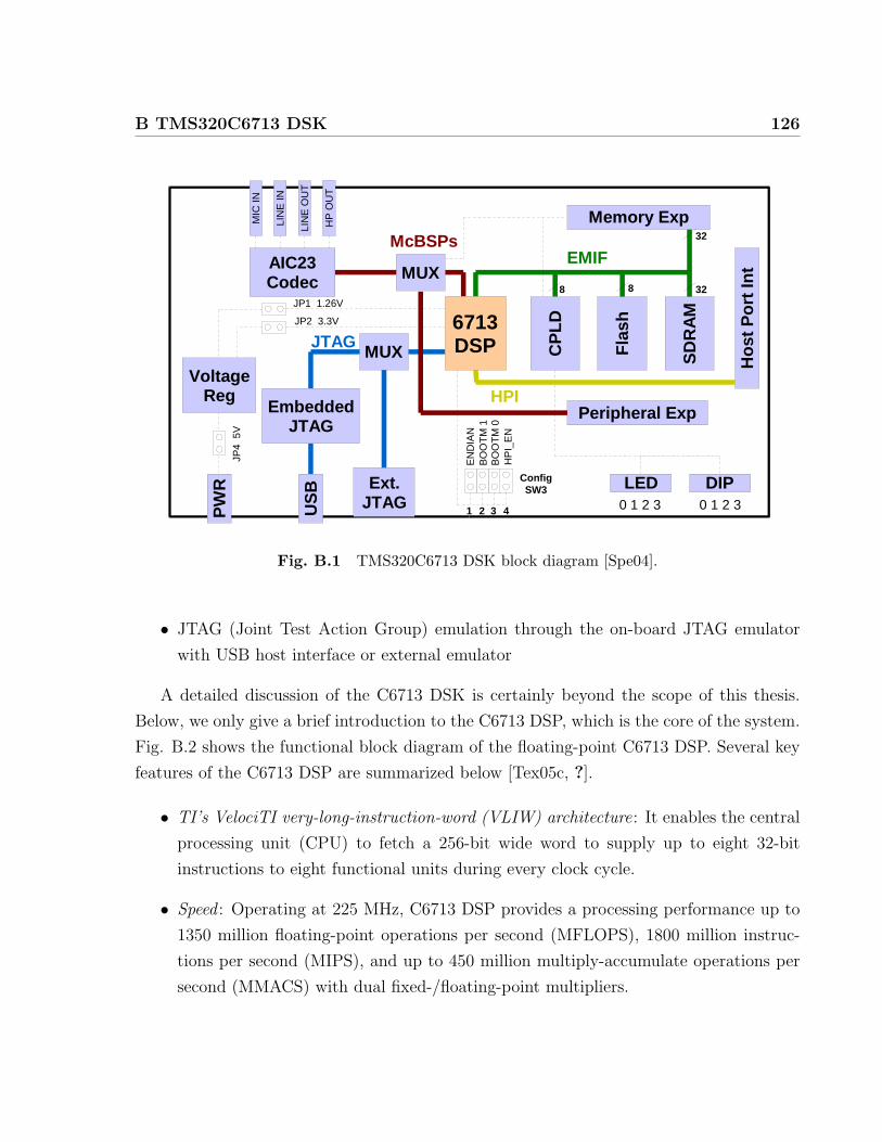
B TMS320C6713 DSK 126
Spectrum Digital, Inc
1-2 TMS320C6713 DSK Module Technical Reference
1.1 Key Features
The C6713 DSK is a low-cost standalone development platform that enables users toevaluate and develop applications for the TI C67xx DSP family. The DSK also servesas a hardware reference design for the TMS320C6713 DSP. Schematics, logicequations and application notes are available to ease hardware development andreduce time to market.
application environments. Key features include:
• A Texas Instruments TMS320C6713 DSP operating at 225 MHz.
• An AIC23 stereo codec
• 16 Mbytes of synchronous DRAM
• 512 Kbytes of non-volatile Flash memory (256 Kbytes usable in default configuration)
• 4 user accessible LEDs and DIP switches
• Software board configuration through registers implemented in CPLD
• Configurable boot options
• Standard expansion connectors for daughter card use
• JTAG emulation through on-board JTAG emulator with USB host interface or external emulator
• Single voltage power supply (+5V)
Ext.JTAG
AIC23Codec
Hos
t Por
t Int
MUX
MUXM
IC IN
LIN
E O
UT
HP
OU
T
LIN
E IN
Peripheral Exp
LED DIP
EMIF
HPI
McBSPs
JTAG
0 1 2 30 1 2 3
CPL
D
Memory ExpPW
R
USB
EmbeddedJTAG
JP1 1.26V
JP2 3.3V
END
IAN
BOO
TM 1
BOO
TM 0
6713DSP
SDR
AM
328
Flas
h
8
1 32
ConfigSW3
32
HPI
_EN
4
VoltageReg
JP4
5V
Fig. B.1 TMS320C6713 DSK block diagram [Spe04].
• JTAG (Joint Test Action Group) emulation through the on-board JTAG emulator
with USB host interface or external emulator
A detailed discussion of the C6713 DSK is certainly beyond the scope of this thesis.
Below, we only give a brief introduction to the C6713 DSP, which is the core of the system.
Fig. B.2 shows the functional block diagram of the floating-point C6713 DSP. Several key
features of the C6713 DSP are summarized below [Tex05c, ?].
• TI’s VelociTI very-long-instruction-word (VLIW) architecture: It enables the central
processing unit (CPU) to fetch a 256-bit wide word to supply up to eight 32-bit
instructions to eight functional units during every clock cycle.
• Speed : Operating at 225 MHz, C6713 DSP provides a processing performance up to
1350 million floating-point operations per second (MFLOPS), 1800 million instruc-
tions per second (MIPS), and up to 450 million multiply-accumulate operations per
second (MMACS) with dual fixed-/floating-point multipliers.
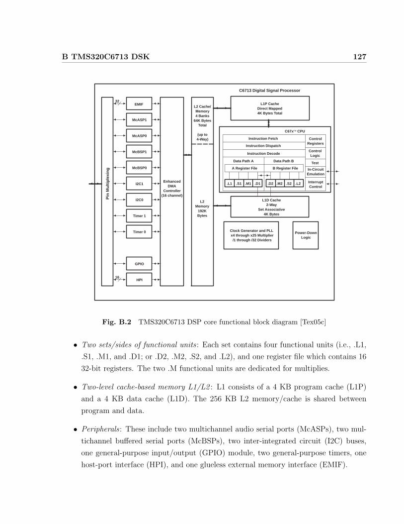
B TMS320C6713 DSK 127
����������� ������� ��� ������� ������ �� ���� �
SPRS186L − DECEMBER 2001 − REVISED NOVEMBER 2005
13POST OFFICE BOX 1443 • HOUSTON, TEXAS 77251−1443
functional block and CPU (DSP core) diagram
Test
C67x CPU
Data Path B
B Register File
Instruction Fetch
Instruction Dispatch
Instruction Decode
Data Path A
A Register File
Power-DownLogic
.L1 .S1 .M1 .S2 .L2
L1P CacheDirect Mapped4K Bytes Total
ControlRegisters
ControlLogic
L1D Cache2-Way
Set Associative4K Bytes
In-CircuitEmulation
InterruptControl
C6713 Digital Signal Processor
EnhancedDMA
Controller(16 channel)
L2 Cache/Memory4 Banks
64K BytesTotal
(up to4-Way)
Clock Generator and PLL x4 through x25 Multiplier/1 through /32 Dividers
L2Memory
192KBytes
EMIF
McASP1
McASP0
McBSP1
McBSP0
I2C1
I2C0
Timer 1
Timer 0
GPIO
HPI
Pin
Mul
tiple
McBSPs interface to:−SPI Control Port−High-Speed TDM Codecs−AC97 Codecs−Serial EEPROM
EMIF interfaces to: −SDRAM−SBSRAM−SRAM, −ROM/Flash, and −I/O devices
McASPs interface to:−I2S Multichannel ADC, DAC, Codec, DIR−DIT: Multiple Outputs
32
16
.M2.D1 .D2
Fig. B.2 TMS320C6713 DSP core functional block diagram [Tex05c]
• Two sets/sides of functional units : Each set contains four functional units (i.e., .L1,
.S1, .M1, and .D1; or .D2, .M2, .S2, and .L2), and one register file which contains 16
32-bit registers. The two .M functional units are dedicated for multiplies.
• Two-level cache-based memory L1/L2 : L1 consists of a 4 KB program cache (L1P)
and a 4 KB data cache (L1D). The 256 KB L2 memory/cache is shared between
program and data.
• Peripherals : These include two multichannel audio serial ports (McASPs), two mul-
tichannel buffered serial ports (McBSPs), two inter-integrated circuit (I2C) buses,
one general-purpose input/output (GPIO) module, two general-purpose timers, one
host-port interface (HPI), and one glueless external memory interface (EMIF).
B TMS320C6713 DSK 128
• Instruction set : C6713 DSK features hardware support for IEEE single and double
precision floating-point operations; 32-bit integer multiply; 8/16/32-bit addressable;
overflow protection, saturation and normalization; etc.
• Other features : These include an enhanced direct-memory-access (EDMA) controller,
a phase-locked loop (PLL) unit, two boot modes (HPI or external asynchronous
ROM), etc.
B.2 Software Overview
TI’s floating-point DSPs are supported by TI’s real-time eXpressDSP softwares and de-
velopment tools [Tex05a], which include three components, namely: the DSP-integrated
development tools in the Code Composer Studio Integrated Development Environment
(CCStudio IDE, or CCS IDE); the eXpressDSP softwares (e.g., DSP/BIOS kernel), and
the TI DSP-based third-party products.
Below, a brief introduction is given to the CCStudio IDE [Tex05a, ?, Tex05b] with focus
on the basic software tools which are useful at different stages of a development, such as
the code creation, debug, and analysis/tuning. A detailed description of these software and
tools would be beyond the scope of the thesis.
B.2.1 Code Creation
Editor/Complier
CCStudio IDE provides a fully integrated code editing environment tuned for C, C++ and
DSP assembly code. In addition to the common features, the source code editor has some
other unique features like column editing and mixed-mode display (i.e., source code plus
disassembled instructions).
CCStudio compile tools shift the burden of optimization from the hand-coded assembly
to the C compiler. One major focus of the C6000 compiler has been VLIW architecture-
specific optimizations/enhancements which include software pipelining, inner and nested
loop optimization, etc.
B TMS320C6713 DSK 129
Available Softwares
• DSP/BIOS : The DSP/BIOS [Tex04b] consists of a real-time kernel, real-time analysis
services, peripheral configuration libraries, and a graphical configuration tool. It
eliminates the need to develop and maintain custom DSP operating systems, and gives
developers the ability to develop embedded real-time software. Application programs
use DSP/BIOS by making calls to the DSP/BIOS Application Programming Interface
(API) [Tex04c], which is divided into modules. All DSP/BIOS modules provide C-
callable interfaces.
Regarding the proposed implementation, we have used API modules such as HST
and STS, and created objects such as the software interrupt. We will have more
discussions on these parts later in Section 7.1.
• Library : Various libraries are provided for different purposes. For example, the Chip
Support Library (CSL) is a set of C functions to manage on-chip peripherals, while
the Board Support Library (BSL) is a set of C APIs used to configure and control
all on-board devices [Tex05a]. Some general-purpose C-callable signal processing
routines are provided by DSP libraries, such as the DSPLIB and IMGLIB [Tex05a].
• TMS320 DSP Algorithm Standard : It defines common programming rules and guide-
lines with a set of programming interfaces that are used consistently by algorithms
across different applications [Tex05a].
• Reference Frameworks : These contain design-ready, reusable C source code [Tex05a].
B.2.2 Debug
Debugger
The CCStudio debugger makes it easy to find and fix errors in real-time embedded appli-
cations by using debug windows/interfaces such as the memory window, registers window,
disassembly window, call stack window, symbol browser, watch window, and command
window. In addition, a probe point can be set to update the connect objects such as a file,
graph, or memory window.
B TMS320C6713 DSK 130
Real-Time Data Exchange
The conventional stop-mode debugging approach exchanges data with the host computer by
using breakpoints to stop the application, which often failed to provide an accurate view
of a system’s real-time operation. TI’s Real-Time Data Exchange (RTDX) technology
offers one solution to this problem by providing real-time, continuous visibility about the
performance of a target application without stopping it. RTDX also allows data to be
streamed with ActiveX-compliant application such as Excel, LabVIEW or Matlab. Host
applications can read either live or saved RTDX data.
B.2.3 Analysis
CCStudio IDE provides various tools to help developers analyze and tune their applications.
Among these is the DSP/BIOS real-time analysis (RTA) tools which provide a unique
visibility into applications. The commonly used DSP/BIOS RTA tools include those to
trace an algorithm by displaying events written to target logs, to monitor performance by
tracking statistics information that reflects the use of target resources, and to handle file
streaming by binding input/output objects to host files. Concerning the tools used in this
work, e.g., Statistics View and Host Channel Control, we will have more discussions in
Section 7.1.

B TMS320C6713 DSK 131
132
References
[ACRLF07] E. Alexandre, L. Cuadra, M. Rosa, and F. Lopez-Ferreras, “Feature selectionfor sound classification in hearing aids through restricted search driven by ge-netic algorithms,” IEEE Trans. Audio, Speech, Lang. Process., vol. 15, no. 8,pp. 2249–2256, Nov. 2007.
[AMB02] J. Ajmera, I. A. Mccowan, and H. Bourlard, “Robust HMM-basedspeech/music segmentation,” in Proc. IEEE Int. Conf. Acoust., Speech, SignalProcess., vol. 1, May 2002, pp. 297–300.
[Ata74] B. S. Atal, “Effectiveness of linear prediction characteristics of the speechwave for automatic speaker identification and verification,” J. Acoust. Soc.Amer., vol. 55, no. 6, pp. 1304–1312, Jun. 1974.
[BALD05] M. Buchler, S. Allegro, S. Launer, and N. Dillier, “Sound classification inhearing aids inspired by auditory scene analysis,” EURASIP J. Applied SignalProcess., vol. 2005, no. 18, pp. 2991–3002, 2005.
[BB04] T. Beierholm and P. M. Baggenstoss, “Speech music discrimination usingclass-specific features,” in Proc. 17th Int. Conf. Pattern Recognition, vol. 2,Aug. 2004, pp. 379–382.
[Bur98] C. J. C. Burges, “A tutorial on support vector machines for pattern recogni-tion,” Data Mining and Knowledge Discovery, vol. 2, no. 2, pp. 121–167, Jun.1998.
[CAS05] W. Chu, M. O. Ahmad, and M. N. S. Swamy, “Modified silence suppressionalgorithms and their performance tests,” in IEEE 48th Midwest SymposiumCircuits Syst., vol. 1, Aug. 2005, pp. 436–439.
[CC06a] W. Chu and B. Champagne, “A noise-robust FFT-based spectrum for audioclassification,” in Proc. IEEE Int. Conf. Acoust., Speech, Signal Process.,vol. 5, May 2006, pp. 213–216.
References 133
[CC06b] W. Chu and B. Champagne, “A simplified early auditory model with appli-cation in audio classification,” Can. J. Elect. Comput. Eng., vol. 31, no. 4,pp. 185–189, Fall 2006.
[CC06c] W. Chu and B. Champagne, “A simplified early auditory model with applica-tion in speech/music classification,” in Proc. IEEE Can. Conf. Elect. Comput.Eng., May 2006, pp. 578–581.
[CC07] W. Chu and B. Champagne, “An improved implementation for an auditory-inspired FFT model with applicaiton in audio classification,” in Proc. IEEEInt. Conf. Multimedia Expo, Jul. 2007, pp. 196–199.
[CC08] W. Chu and B. Champagne, “A noise-robust FFT-based auditory spectrumwith application in audio classification,” IEEE Trans. Audio, Speech, Lang.Process., vol. 1, pp. 137–150, Jan. 2008.
[CLZC03] R. Cai, L. Lu, H.-J. Zhang, and L.-H. Cai, “Highlight sound effects detectionin audio stream,” in Proc. Int. Conf. Multimedia Expo, vol. 3, Jul. 2003, pp.37–40.
[CPLT99] M. J. Carey, E. S. Parris, and H. Lloyd-Thomas, “A comparison of featuresfor speech, music discrimination,” in Proc. IEEE Int. Conf. Acoust., Speech,Signal Process., vol. 1, Mar. 1999, pp. 149–152.
[CS01] K. Crammer and Y. Singer, “On the algorithmic implementation of multi-class kernel-based vector machines,” J. Mach. Learn. Res., vol. 2, pp. 265–292,Dec. 2001.
[CV95] C. Cortes and V. Vapnik, “Support-vector networks,” Machine Learning,vol. 20, no. 3, pp. 273–297, Sep. 1995.
[DM80] S. Davis and P. Mermelstein, “Comparison of parametric representationsfor monosyllabic word recognition in continuously spoken sentences,” IEEETrans. Acoust., Speech, Signal Process., vol. 28, no. 4, pp. 357– 366, Aug.1980.
[ECS03] M. Elhilali, T. Chi, and S. Shamma, “A spectro-temporal modulation in-dex (STMI) for assessment of speech intelligibility,” Speech Communication,vol. 41, pp. 331–348, Oct. 2003.
[EKR04] S. Esmaili, S. Krishnan, and K. Raahemifar, “Content based audio classifi-cation and retrieval using joint time-frequency analysis,” in Proc. IEEE Int.Conf. Acoust., Speech, Signal Process., vol. 5, May 2004, pp. 665–668.
References 134
[EMKPK00] K. El-Maleh, M. Klein, G. Petrucci, and P. Kabal, “Speech/music discrimina-tion for multimedia applications,” in Proc. IEEE Int. Conf. Acoust., Speech,Signal Process., vol. 6, Jun. 2000, pp. 2445–2448.
[FU01] J. Foote and S. Uchihashi, “The beat spectrum: a new approach to rhythmanalysis,” in Proc. IEEE Int. Conf. Multimedia Expo, Aug. 2001, pp. 881–884.
[Fuk90] K. Fukunaga, Introduction to Statistical Pattern Recognition, 2nd ed. Boston:Academic Press, 1990.
[FZWL03] Z. Feng, Y. Zhou, L. Wu, and Z. Li, “Audio classification based on maximumentropy model,” in Proc. Int. Conf. Multimedia Expo, vol. 1, Jul. 2003, pp.745–748.
[GL03] G. Guo and S. Z. Li, “Content-based audio classification and retrieval bysupport vector machines,” IEEE Trans. Neural Networks, vol. 14, no. 1, pp.209–215, Jan. 2003.
[GL04] M. M. Goodwin and J. Laroche, “A dynamic programming approach to audiosegmentation and speech/music discrimination,” in Proc. IEEE Int. Conf.Acoust., Speech, Signal Process., vol. 4, May 2004, pp. 309–312.
[GZL01] G. Guo, H.-J. Zhang, and S. Z. Li;, “Boosting for content-based audio clas-sification and retrieval: an evaluation,” in Proc. IEEE Int. Conf. MultimediaExpo, Aug. 2001, pp. 997–1000.
[HH04] R. Huang and J. H. L. Hansen, “Advances in unsupervised audio segmenta-tion for the broadcast news and NGSW corpora,” in Proc. IEEE Int. Conf.Acoust., Speech, Signal Process., vol. 1, May 2004, pp. 741–744.
[ITU96] ITU-T Recommendation G.729, Annex B, “A silence compression scheme forG.729 optimization for terminals conforming to Recommendation V.70,” Nov.1996.
[JLZ00] H. Jiang, T. Lin, and H.-J. Zhang, “Video segmentation with the assistanceof audio content analysis,” in Proc. IEEE Int. Conf. Multimedia Expo, vol. 3,Jul. 2000, pp. 1507 – 1510.
[JOMM02] R. Jarina, N. O’Connor, S. Marlow, and N. Murphy, “Rhythm detection forspeech-music discrimination in MPEG compressed domain,” in Proc. 14thInt. Conf. Digital Signal Process., vol. 1, Jul. 2002, pp. 129–132.
[Kat95] J. M. Kates, “Classification of background noises for hearing-aid applica-tions,” J. Acoust. Soc. Amer., vol. 97, no. 1, pp. 461–470, Jan. 1995.
References 135
[KMS04] H.-G. Kim, N. Moreau, and T. Sikora, “Audio classification based on MPEG-7 spectral basis representations,” IEEE Trans. Circuits Syst. Video Technol.,vol. 14, no. 5, pp. 716–725, May 2004.
[KQG04] S. Kiranyaz, A. F. Qureshi, and M. Gabbouj, “A fuzzy approach towardsperceptual classification and segmentation of MP3/AAC audio,” in Proc. 1stInt. Symposium Control, Communications, Signal Process., 2004, pp. 727–730.
[Lay03] D. C. Lay, Linear Algebra and its Applications, 3rd ed. Boston, Mass.:Addison-Wesley, 2003.
[LCTC05] C.-C. Lin, S.-H. Chen, T.-K. Truong, and Y. Chang;, “Audio classificationand categorization based on wavelets and support vector machine,” IEEETrans. Speech Audio Process., vol. 13, no. 5, pp. 644–651, Sep. 2005.
[LD04] Y. Li and C. Dorai, “SVM-based audio classification for instructional videoanalysis,” in Proc. IEEE Int. Conf. Acoustics, Speech, Signal Processing,vol. 5, May 2004, pp. 897–900.
[LH00a] Z. Liu and Q. Huang, “Content-based indexing and retrieval-by-example inaudio,” in Proc. IEEE Int. Conf. Multimedia Expo, vol. 2, Jul.-Aug. 2000, pp.877–880.
[LH00b] G. Lu and T. Hankinson, “An investigation of automatic audio classificationand segmentation,” in Proc. IEEE Int. Conf. Signal Process., vol. 2, Aug.2000, pp. 776–781.
[LHWC97] Z. Liu, J. Huang, Y. Wang, and T. Chuan, “Audio feature extraction andanalysis for scene classification,” in Proc. IEEE Workshop Multimedia SignalProcess., Jun. 1997, pp. 343–348.
[Li00] S. Z. Li, “Content-based audio classification and retrieval using the nearestfeature line method,” IEEE Trans. Speech Audio Process., vol. 8, no. 5, pp.619–625, Sep. 2000.
[LS04] W.-N. Lie and C.-K. Su, “Content-based retrieval of MP3 songs based onquery by singing,” in Proc. IEEE Int. Conf. Acoust., Speech, Signal Process.,vol. 5, May 2004, pp. 929–932.
[LZJ02] L. Lu, H.-J. Zhang, and H. Jiang;, “Content analysis for audio classificationand segmentation,” IEEE Trans. Speech Audio Process., vol. 10, no. 7, pp.504–516, Oct. 2002.
References 136
[Mey70] P. L. Meyer, Introductory Probability and Statistical Applications, 2nd ed.MA: Addison-Wesley, 1970.
[MR00] P. J. Moreno and R. Rifkin, “Using the fisher kernel method for web audioclassification,” in Proc. IEEE Int. Conf. Acoust., Speech, Signal Process.,vol. 6, Jun. 2000, pp. 2417–2420.
[MSS04] N. Mesgarani, S. Shamma, and M. Slaney, “Speech discrimination based onmultiscale spectro-temporal modulations,” in Proc. IEEE Int. Conf. Acoust.,Speech, Signal Process., vol. 1, May 2004, pp. 601–604.
[Neu] Neural Systems Laboratory, University of Maryland. NSL Matlab Toolbox.[Online]. Available: http://www.isr.umd.edu/Labs/NSL/nsl.html. [CitedMay 2005].
[NHK05] N. Nitanda, M. Haseyama, and H. Kitajima, “Accurate audio-segment clas-sification using feature extraction matrix,” in Proc. IEEE Int. Conf. Acoust.,Speech, Signal Process., vol. 3, Mar. 2005, pp. 261–264.
[NL04] P. Nordqvist and A. Leijon, “An efficient robust sound classification algorithmfor hearing aids,” J. Acoust. Soc. Amer., vol. 115, no. 6, pp. 3033–3041, Jun.2004.
[NL05] T. L. Nwe and H. Li, “Broadcast news segmentation by audio type analysis,”in Proc. IEEE Int. Conf. Acoust., Speech, Signal Process., vol. 2, Mar. 2005,pp. 1065–1068.
[NLS+99] Y. Nakajima, Y. Lu, M. Sugano, A. Yoneyama, and H. Y. A. Kurematsu, “Afast audio classification from MPEG coded data,” in Proc. IEEE Int. Conf.Acoust., Speech, Signal Process., vol. 6, Mar. 1999, pp. 3005–3008.
[O’S00] D. O’Shaughnessy, Speech Communications-Human and Machines, 2nd ed.New York: IEEE Press, 2000.
[OSB99] A. V. Oppenheim, R. W. Schafer, J. R. Buck, Discrete-Time Signal Process-ing, 2nd ed. Englewood Cliffs, N. J.: Prentice-Hall, 1999.
[Oti] http://adapto.oticon.com. [Cited Apr. 2006].
[Pho] http://www.phonak.com. [Cited Apr. 2006].
[PP02] A. Papoulis and S. U. Pillai, Probability, Random Variables, and StochasticProcesses, 4th ed. New York: McGraw-Hill, 2002.
References 137
[PRAO03] J. Pinquier, J.-L. Rouas, and R. Andre-Obrecht, “A fusion study inspeech/music classification,” in Proc. Int. Conf. Multimedia Expo, vol. 1, Jul.2003, pp. 409–412.
[PT05] C. Panagiotakis and G. Tziritas, “A speech/music discriminator based onRMS and zero-crossings,” IEEE Trans. Multimedia, vol. 7, pp. 155–166, Feb.2005.
[Qia97] R.-Y. Qiao, “Mixed wideband speech and music coding using a speech/musicdiscriminator,” in Proc. IEEE Region 10 Annu. Conf. Speech Image Technol.for Comput. Telecomm., vol. 2, Dec. 1997, pp. 605–608.
[Qui93] J. R. Quinlan, C4.5:programs for machine learning. San Mateo, CA: MorganKaufmann, 1993.
[RA04] S. Ravindran and D. Anderson, “Low-power audio classification for ubiquitoussensor networks,” in Proc. IEEE Int. Conf. Acoust., Speech, Signal Process.,vol. 4, May 2004, pp. 337–340.
[RA05] S. Ravindran and D. V. Anderson, “Audio classification and scene recognitionand for hearing aids,” in Proc. IEEE Int. Symposium Circuits Systems, vol. 2,May 2005, pp. 860–863.
[Rab89] L. R. Rabiner, “A tutorial on hidden Markov models and selected applicationsin speech recognition,” in Proc. IEEE, vol. 77, Feb. 1989, pp. 257–286.
[RJ93] L. Rabiner and B.-H. Juang, Fundamentals of Speech Recognition. EnglewoodCliffs, NJ: Prentice-Hall, 1993.
[RN03] S. J. Russell and P. Norvig, Artificial Intelligence: A Modern Approach,2nd ed. Upper Saddle River, N.J.: Prentice Hall, 2003.
[RS78] L. R. Rabiner and R. W. Schafer, Digital processing of speech signals. En-glewood Cliffs, N.J.: Prentice-Hall, 1978.
[RSA05] S. Ravindran, K. Schlemmer, and D. V. Anderson, “A physiologically in-spired method for audio classification,” EURASIP J. Applied Signal Process-ing, no. 9, pp. 1374–1381, 2005.
[Ru00] P.-W. Ru, “Perception-based multi-resolution auditory processing of acousticsignals,” Ph.D. dissertation, University of Maryland, 2000.
[SA04] C. Senac and E. Ambikairajah, “Audio indexing using feature warping andfusion techniques,” in Proc. IEEE 6th Workshop Multimedia Signal Process.,Sep. 2004, pp. 359–362.
References 138
[Sau96] J. Saunders, “Real-time discrimination of broadcast speech/music,” in Proc.IEEE Int. Conf. Acoust., Speech, Signal Process., vol. 2, May 1996, pp. 993–996.
[Sch98] E. D. Scheirer, “Tempo and beat analysis of acoustic musical signals,” J.Acoust. Soc. Amer., vol. 103, no. 1, pp. 588–601, Jan. 1998.
[Sch00] F. Schwenker, “Hierarchical support vector machines for multi-class patternrecognition,” in Proc. IEEE 4th Int. Conf. Knowledge-Based Intell. Eng. Syst.Allied Technol., vol. 2, Aug. 2000, p. 561–565.
[Sla] M. Slaney. Auditory Toolbox: A Matlab Toolbox for Auditory ModelingWork (Version 2). Interval Research Corporation, Tech. Rep. 1998-010, 1998.[Online]. Available: http://www.slaney.org/malcolm/pubs.html. [Cited Jul.2006].
[Spe04] TMS320C6713 DSK Technical Reference, Spectrum Digital, Stanfford, TX,Jan. 2004.
[SS97] E. Scheirer and M. Slaney, “Construction and evaluation of a robust multifea-ture speech/music discriminator,” in Proc. IEEE Int. Conf. Acoust., Speech,Signal Process., vol. 2, Apr. 1997, pp. 1331–1334.
[TC00] G. Tzanetakis and F. Cook, “Sound analysis using MPEG compressed audio,”in Proc. IEEE Int. Conf. Acoust., Speech, Signal Process., vol. 2, Jun. 2000,pp. 761–764.
[Tex02] TMS320C67x FastRTS Library Programmer’s Reference, Texas Instruments,Dallas, TX, Oct. 2002.
[Tex04b] TMS320 DSP/BIOS User’s Guide, Texas Instruments, Dallas, TX, Apr. 2004.
[Tex04c] TMS320C6000 DSP/BIOS Application Programming Interface (API) Refer-ence Guide, Texas Instruments, Dallas, TX, Apr. 2004.
[Tex04d] TMS320C6000 Optimizing Compiler User’s Guide, Texas Instruments, Dal-las, TX, May 2004.
[Tex05a] Code Composer Studio IDE Getting Started Guide, Texas Instruments, Dallas,TX, May 2005.
[Tex05b] TMS320C6000 Code Composer Studio IDE Help, Texas Instruments, Dallas,TX, May 2005.
References 139
[Tex05c] TMS320C6713 Floating-Point Digital Signal Processor, Texas Instruments,Dallas, TX, Nov. 2005.
[Tex06] TMS320C67x DSP Library Programmer’s Reference Guide, Texas Instru-ments, Dallas, TX, Mar. 2006.
[TIA98] TIA/EIA/IS-727, “TDMA cellular/pcs-radio interface–minimum perfor-mance standards for discontinuous transmission operation of mobile stations,”Jun. 1998.
[TJHA05] I. Tsochantaridis, T. Joachims, T. Hofmann, and Y. Altun, “Large marginmethods for structured and interdependent output variables,” J. Mach. Learn.Res., vol. 6, pp. 1453–1484, Sep. 2005.
[TRRL00] L. Tancerel, S. Ragot, V. T. Ruoppila, and R. Lefebvre, “Combined speechand audio coding by discrimination,” in Proc. IEEE Workshop Speech Coding,Sep. 2000, pp. 154–156.
[UKJ05] K. Umapathy, S. Krishnan, and S. Jimaa, “Multigroup classification of audiosignals using time-frequency parameters,” IEEE Trans. Multimedia, vol. 7,no. 2, pp. 308–315, Apr. 2005.
[VBDT99] M. Viswanathan, H. S. M. Beigi, S. Dharanipragada, and A. Tritschler, “Re-trieval from spoken documents using content and speaker information,” inProc. 5th Int. Conf. Document Analysis Recognition, Sep. 1999, pp. 567–572.
[VSTJMs] A. Varga, H. J. M. Steeneken, M. Tomlinson, and D. Jones, “The NOISEX-92study on the effect of additive noise on automatic speech recognition,” 1992,Documentation Included in the NOISEX-92 CD-ROMs.
[WBKW96] E. Wold, T. Blum, D. Keislar, and J. Wheaten, “Content-based classification,search, and retrieval of audio,” IEEE Multimedia, vol. 3, no. 3, pp. 27–36, Fall1996.
[WGY03] W. Q. Wang, W. Gao, and D. W. Ying, “A fast and robust speech/musicdiscrimination approach,” in Proc. 2003 Joint Conf. of the 4th Int. Conf.Information, Communications, Signal Process. and the 4th Pacific Rim Conf.Multimedia, vol. 3, Dec. 2003, pp. 1325–1329.
[WHJ+98] P. C. Woodland, T. Hain, S. E. Johnson, T. R. Niesler, and A. T. S. J.Young, “Experiments in broadcast news transcription,” in Proc. IEEE Int.Conf. Acoust., Speech, Signal Process., vol. 2, May 1998, pp. 909–912.
References 140
[WLH00] Y. Wang, Z. Liu, and J.-C. Huang, “Multimedia content analysis using bothaudio and visual clues,” IEEE Signal Process. Mag., vol. 17, no. 6, pp. 12–36,Nov. 2000.
[WS94] K. Wang and S. Shamma, “Self-normalization and noise-robustness in earlyauditory representations,” IEEE Trans. Speech Audio Process., vol. 2, no. 3,pp. 421–435, Jul. 1994.
[XMS05] C. Xu, N. C. Maddage, and X. Shao, “Automatic music classification andsummarization,” IEEE Trans. Speech Audio Process., vol. 13, no. 3, pp. 441–450, May 2005.
[XRDH03] Z. Xiong, R. Radhakrishnan, A. Divakaran, and T. S. Huang, “ComparingMFCC and MPEG-7 audio features for feature extraction, maximum likeli-hood HMM and entropic prior HMM for sports audio classification,” in Proc.IEEE Int. Conf. Acoust., Speech, Signal Process., vol. 5, Apr. 2003, pp. 628–631.
[YBF+97] S. J. Young, M. G. Brown, J. T. Foote, G. J. F. Jones, and K. S.Jones,“Acoustic indexing for multimedia retrieval and browsing,” in Proc. IEEEInt. Conf. Acoust., Speech, Signal Process., vol. 1, Apr. 1997, pp. 199–202.
[ZBC03] M. Zhao, J. Bu, and C. Chen, “Audio and video combined for home videoabstraction,” in Proc. IEEE Int. Conf. Acoust., Speech, Signal Process., vol. 5,Apr. 2003, pp. 620–623.
[ZC01] T. Zhang and C.-C. Jay Kuo, “Audio content analysis for online audiovisualdata segmentation and classification,” IEEE Trans. Speech Audio Process.,vol. 9, no. 4, pp. 441–457, May 2001.
[Zha00] G. Zhang, “Neural networks for classification: a survey,” IEEE Trans. Syst.,Man, Cybern. C, Appl. Rev., vol. 30, no. 4, pp. 451–462, Nov. 2000.
[ZK99] T. Zhang and C.-C. J. Kuo, “Hierarchical classification of audio data forarchiving and retrieving,” in Proc. IEEE Int. Conf. Acoust., Speech, SignalProcess., vol. 6, Mar. 1999, pp. 3001–3004.
[ZZ03] Y. Zhu and D. Zhou, “Scene change detection based on audio and video con-tent analysis,” in Proc. 5th Int. Conf. Computational Intelligence MultimediaApplications, Sep. 2003, pp. 229–234.
[ZZ04] Y. Zhang and J. Zhou, “Audio segmentation based on multi-scale audio clas-sification,” in Proc. IEEE Int. Conf. Acoust., Speech, Signal Process., vol. 4,May 2004, pp. 349–352.