Embed Size (px)
Citation preview
1995 NCTU/CSIE DSPLAB C.M..LIU
P.1Audio Coding
FundamentalsQuantizationWaveform CodingSubband Coding
1995 NCTU/CSIE DSPLAB C.M..LIU
P.21. Fundamentals
IntroductionData Redundancy
Coding RedundancySpatial/Temporal RedundancyPerceptual Redundancy
Compression ModelsA General Compression System ModelThe Sourc/Channel e Encoder and Decoder
Information TheoryInformationEntropyConditional Information & EntropyMutual Information
1995 NCTU/CSIE DSPLAB C.M..LIU
P.31.1 Introduction
CompressionReduce the amount of data required to represent a media
Why CompressionStereo Audio– 16 bits for 96 dB– 44.1 k sample rate– 176.4 k bytes per second and 10Mbytes for a minute
Video– 525 x 360 x 30 x 3 = 17 MB/s or 136 Mb/s– 1000 Mbytes for a minute
Compression is necessary for storage, communication, ...
1995 NCTU/CSIE DSPLAB C.M..LIU
P.41.1 Introduction (c.1)
Advantages of Digital over Analog SignalsProcessing Flexibility and FacilityEase of Precision ControlHigher Signal-to-Noise Resistance
Techniques to Compress DataData RedundanciesPerceptual EffectsApplications Requirements
StandardsSpeed up the advance of related technologyIncrease the compatibilityThe landmarks of technical developments.
1995 NCTU/CSIE DSPLAB C.M..LIU
P.51.1 Introduction (c.2)
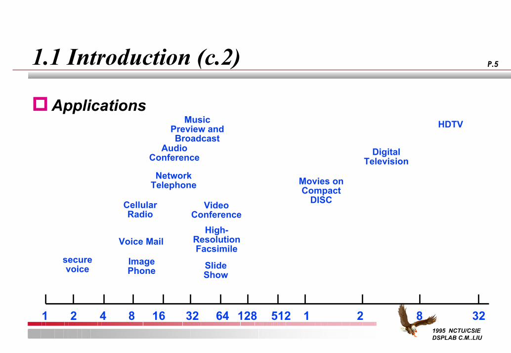
Applications
1 2 4 8 16 32 64 128 512 1
secure voice
Cellular Radio
Voice Mail
Image Phone Slide
Show
High-Resolution Facsimile
Video Conference
Network Telephone
Audio Conference
Music Preview and Broadcast
Movies on Compact
DISC
Digital Television
2 8
HDTV
32
1995 NCTU/CSIE DSPLAB C.M..LIU
P.61.1 Introduction (c.3)
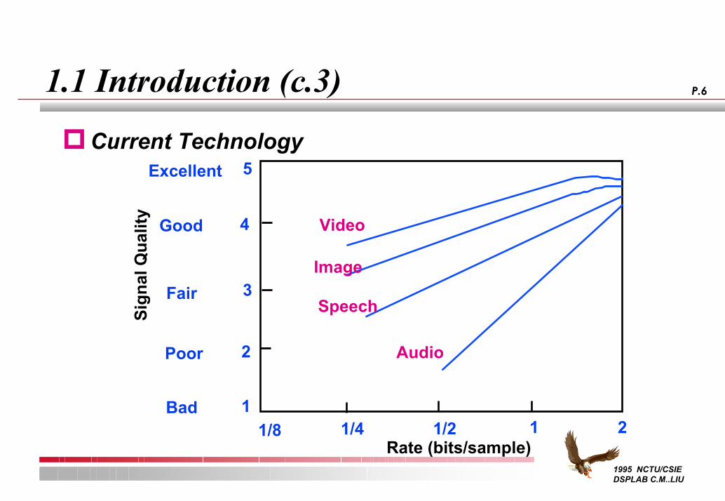
Current Technology5
Audio
Speech
Image
Video
Excellent
Sign
al Q
ualit
y 4Good
3Fair
2Poor
1Bad21/4 1/2 1
Rate (bits/sample)1/8
1995 NCTU/CSIE DSPLAB C.M..LIU
P.71.2 Redundancy
Data v.s. InformationCoding RedundancyInterdata RedundancyPerceptual Redundancy
1995 NCTU/CSIE DSPLAB C.M..LIU
P.81.2 Redundancy-- Data v.s. Information
Data CompressionProcess of reducing the amount of data required to represent a given quantity of information.
Data v.s. InformationData are means by which information is conveyed.
Data RedundancyThe part of data that contains no relevent informationNot an abstract concept but a mathematically quantifiable entity
1995 NCTU/CSIE DSPLAB C.M..LIU
P.91.2 Redundancies-- Data v.s. Information(c.1)
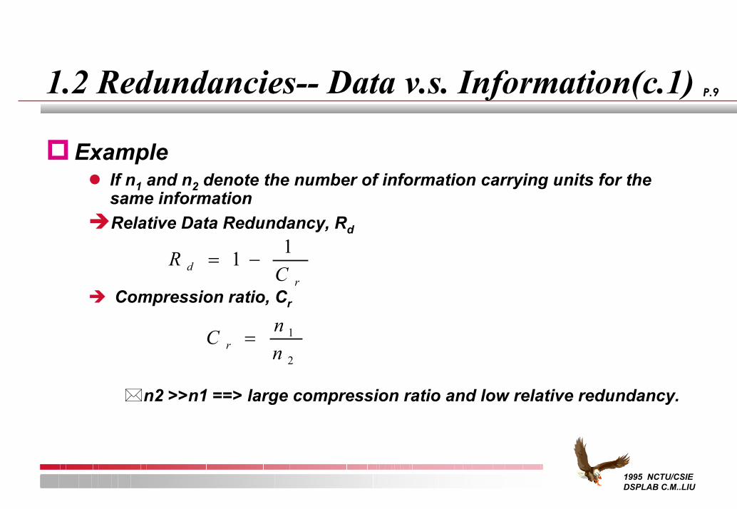
ExampleIf n1 and n2 denote the number of information carrying units for the same informationRelative Data Redundancy, Rd
Compression ratio, Cr
n2 >>n1 ==> large compression ratio and low relative redundancy.
RCd
r
= −1 1
C nnr = 1
2
1995 NCTU/CSIE DSPLAB C.M..LIU
P.101.2 Redundancy-- Coding Redundancy
Redundancy SourcesThe number of bits used to represent different symbols needs not be the same.
Assume that the occurance probability of each symbol rkis p(rk) and the number of bits used to represent rk is l(rk)
Average number of bits for a symbol is
Variable Length CodingAssign fewer bits to the more probable symbols for compression.
L l r p ravg kk
k= ∑ ( ) ( )
1995 NCTU/CSIE DSPLAB C.M..LIU
P.111.2 Redundancy-- Coding Redundancy(c.1)
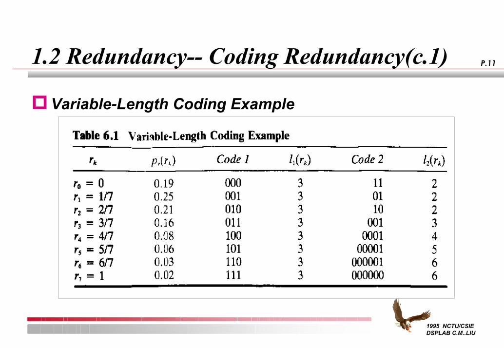
Variable-Length Coding Example
1995 NCTU/CSIE DSPLAB C.M..LIU
P.121.2 Redundancy-- Coding Redundancy(c.2)
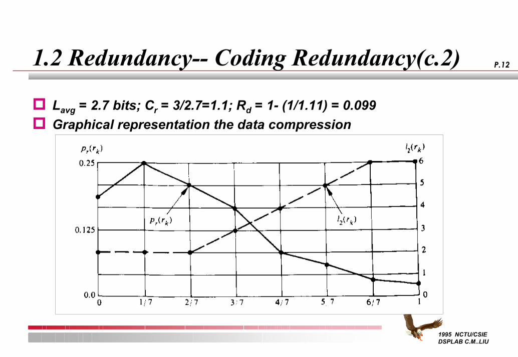
Lavg = 2.7 bits; Cr = 3/2.7=1.1; Rd = 1- (1/1.11) = 0.099Graphical representation the data compression
1995 NCTU/CSIE DSPLAB C.M..LIU
P.131.2 Redundancy-- Interdata Redundancy
There is correlation between dataThe value of a data can be predicted from its neighbors
The information carried by individual data is relatively small.
Other namesInterpixel Redundancy, Spatial Redundancy, Temporal Redundancy
Ex.Run-length coding
1995 NCTU/CSIE DSPLAB C.M..LIU
P.141.2 Redundancy-- Perceptual Redundancy
Certain information is not essential for normal perceptual processingExample:
Sharpe edges in an image.Stronger sounds mask the weaker sounds.
Other namesPsychovisual redundancyPsychoacoustic redundancy
1995 NCTU/CSIE DSPLAB C.M..LIU
P.151.3 Compression Models
A General Compression System ModelThe Source Encoder and DecoderThe Channel Encoder and Decoder
1995 NCTU/CSIE DSPLAB C.M..LIU
P.16
1.3 Compression Models-- A General Compression System Model
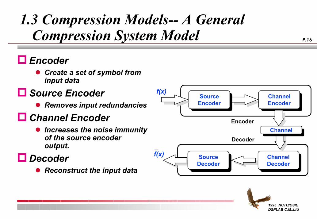
EncoderCreate a set of symbol from input data
Source EncoderRemoves input redundancies
Channel EncoderIncreases the noise immunity of the source encoder output.
DecoderReconstruct the input data
Source EncoderSource
Encoder
f(x)
f(x)
Encoder
Decoder
ChannelDecoder
ChannelDecoder
ChannelEncoder
ChannelEncoder
ChannelChannel
Source DecoderSource
Decoder
1995 NCTU/CSIE DSPLAB C.M..LIU
P.17
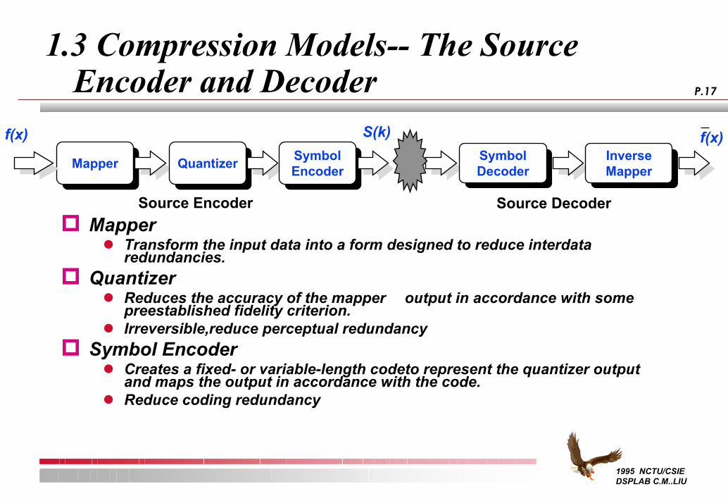
1.3 Compression Models-- The Source Encoder and Decoder
S(k)f(x) f(x)
MapperTransform the input data into a form designed to reduce interdataredundancies.
QuantizerReduces the accuracy of the mapper output in accordance with somepreestablished fidelity criterion.Irreversible,reduce perceptual redundancy
Symbol EncoderCreates a fixed- or variable-length codeto represent the quantizer output and maps the output in accordance with the code.Reduce coding redundancy
MapperMapper
Source Encoder Source Decoder
QuantizerQuantizer SymbolEncoderSymbolEncoder
Symbol DecoderSymbol Decoder
InverseMapper
InverseMapper
1995 NCTU/CSIE DSPLAB C.M..LIU
P.18
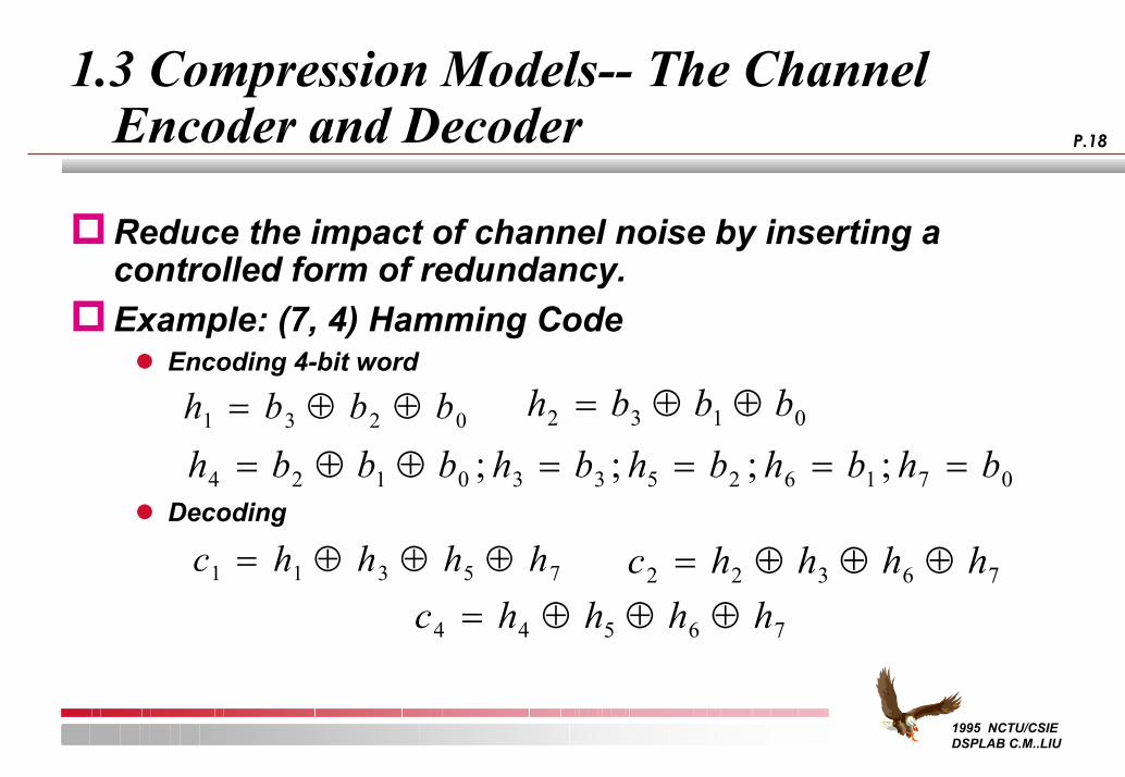
1.3 Compression Models-- The Channel Encoder and Decoder
Reduce the impact of channel noise by inserting a controlled form of redundancy.Example: (7, 4) Hamming Code
Encoding 4-bit word
Decoding
h b b b1 3 2 0= ⊕ ⊕ h b b b2 3 1 0= ⊕ ⊕
h b b b h b h b h b h b4 2 1 0 3 3 5 2 6 1 7 0= ⊕ ⊕ = = = =; ; ; ;
c h h h h1 1 3 5 7= ⊕ ⊕ ⊕ c h h h h2 2 3 6 7= ⊕ ⊕ ⊕c h h h h4 4 5 6 7= ⊕ ⊕ ⊕
1995 NCTU/CSIE DSPLAB C.M..LIU
P.191.4 Information Theory
InformationEntropyConditional Information & EntropyMutual Information
1995 NCTU/CSIE DSPLAB C.M..LIU
P.201.4 Information Theory (c.1)
IntroductionWhat does Information Theory talk about ?– The field of information theory is concerned with the amount of
uncertainty associated with the outcome of an experiment .– The amount of information we receive when the outcome is known
depends upon how much uncertainty there was about its occurren
1995 NCTU/CSIE DSPLAB C.M..LIU
P.211.4 Information Theory (c.2)
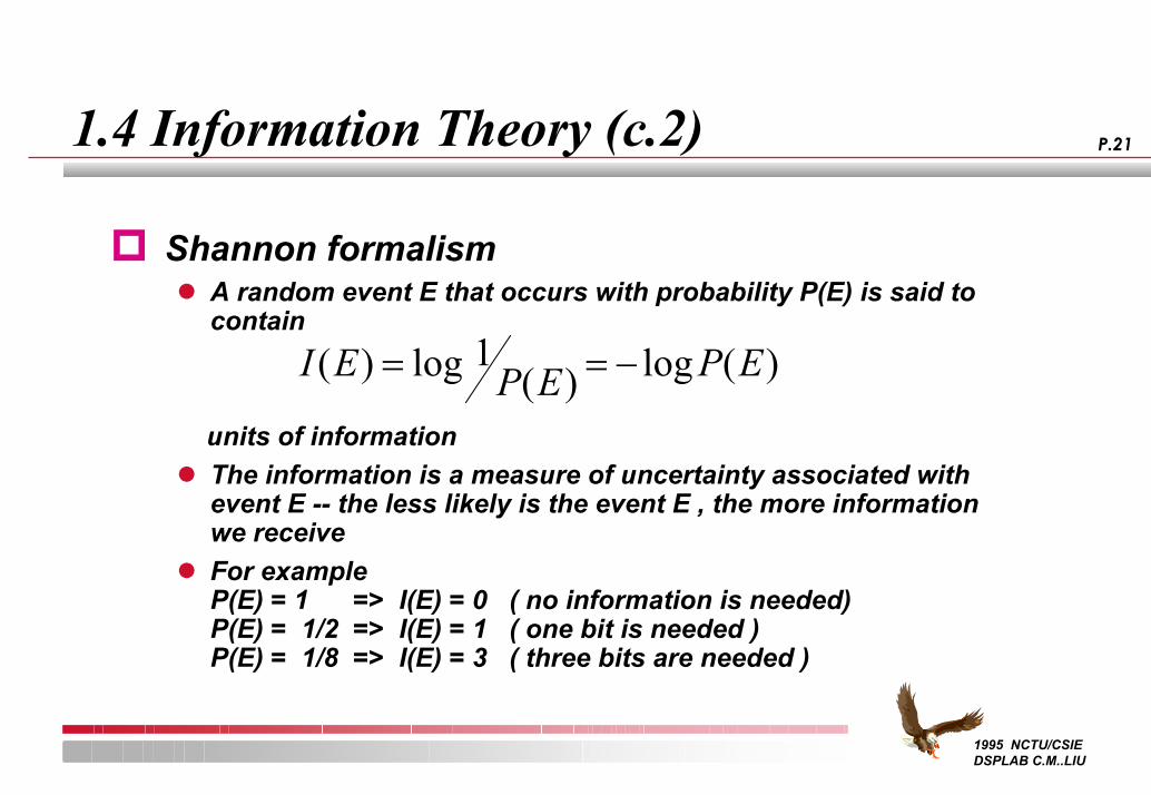
Shannon formalismA random event E that occurs with probability P(E) is said to contain
units of information The information is a measure of uncertainty associated with event E -- the less likely is the event E , the more information we receiveFor example P(E) = 1 => I(E) = 0 ( no information is needed) P(E) = 1/2 => I(E) = 1 ( one bit is needed ) P(E) = 1/8 => I(E) = 3 ( three bits are needed )
I E P E P E( ) log ( ) log ( )= = −1
1995 NCTU/CSIE DSPLAB C.M..LIU
P.221.4 Information Theory (c.3)
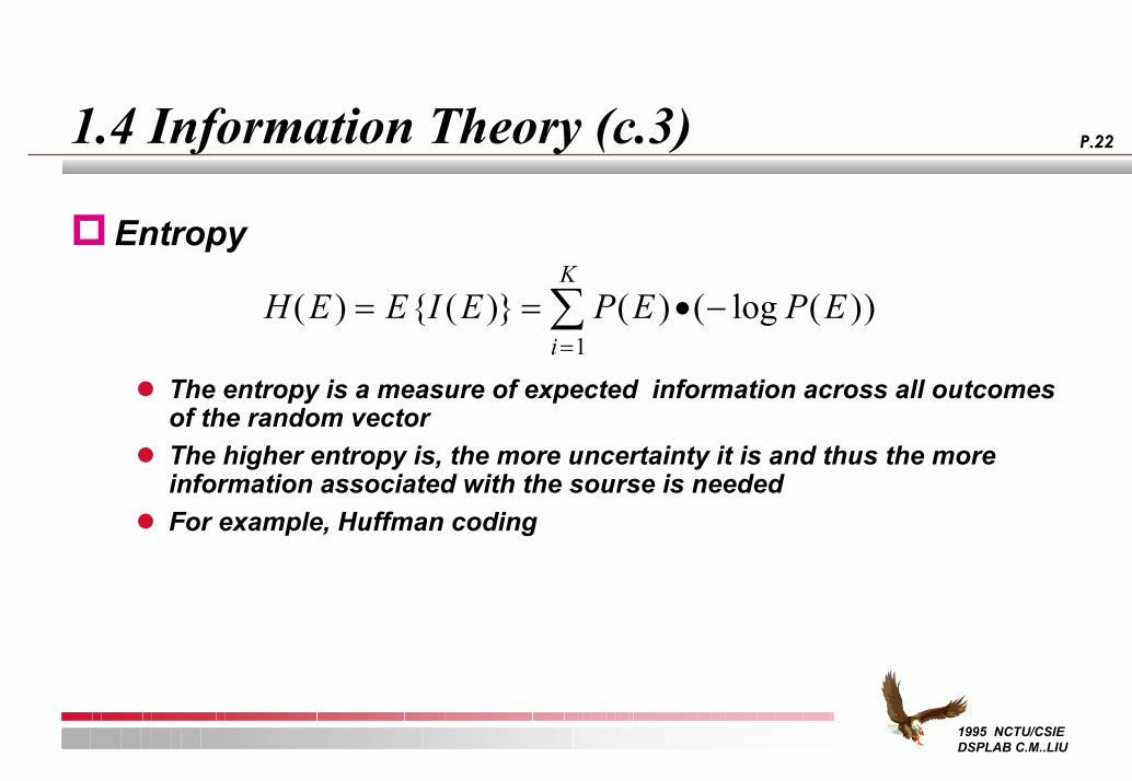
H E E I E P E P Ei
K( ) { ( )} ( ) ( log ( ))= = • −
=∑
1
Entropy
The entropy is a measure of expected information across all outcomes of the random vector The higher entropy is, the more uncertainty it is and thus the more information associated with the sourse is neededFor example, Huffman coding
1995 NCTU/CSIE DSPLAB C.M..LIU
P.231.4 Information Theory (c.4)
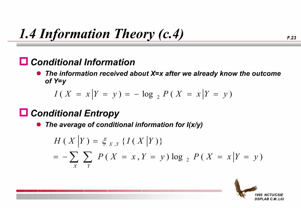
Conditional InformationThe information received about X=x after we already know the outcome of Y=y
Conditional EntropyThe average of conditional information for I(x/y)
I X x Y y P X x Y y( ) log ( )= = = − = =2
H X Y I X Y
P X x Y y P X x Y yX Y
YX
( ) { ( )}
( , ) log ( ),=
= − = = = =∑∑ξ
2
1995 NCTU/CSIE DSPLAB C.M..LIU
P.241.4 Information Theory (c.5)
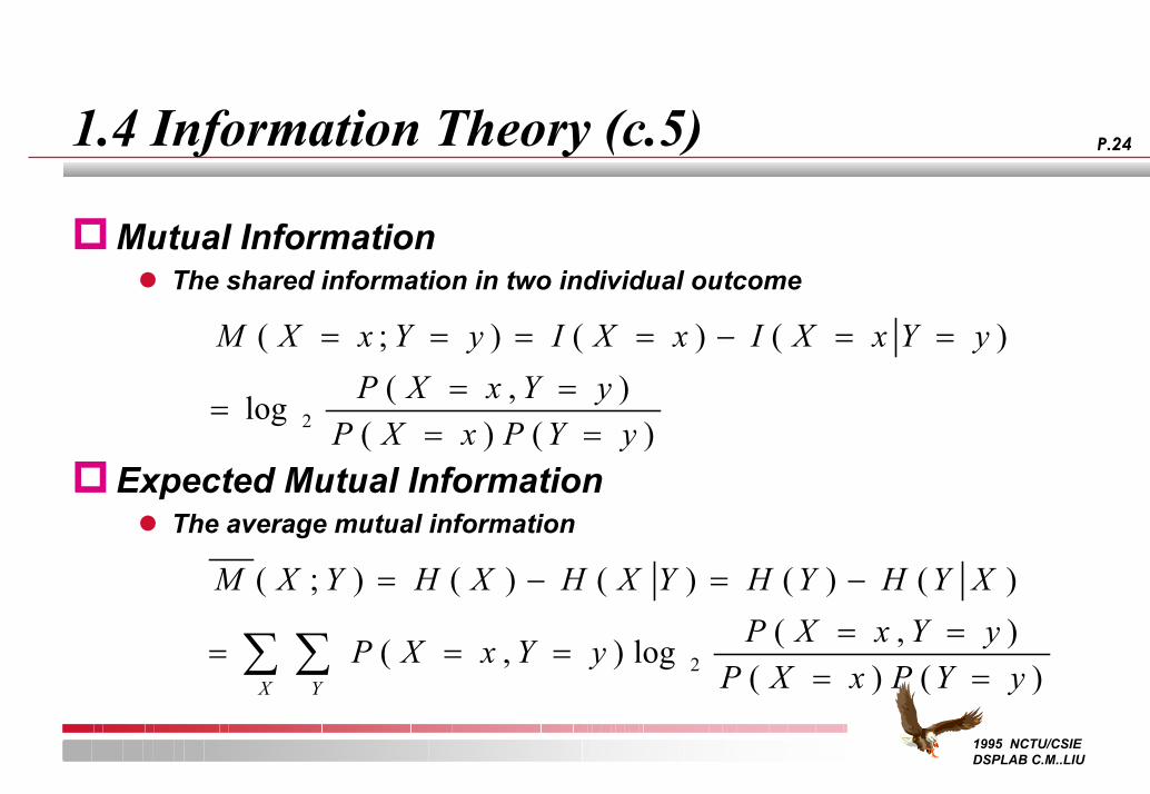
Mutual Information The shared information in two individual outcome
Expected Mutual InformationThe average mutual information
M X x Y y I X x I X x Y yP X x Y yP X x P Y y
( ; ) ( ) ( )
log ( , )( ) ( )
= = = = − = =
== =
= =2
M X Y H X H X Y H Y H Y X
P X x Y y P X x Y yP X x P Y yYX
( ; ) ( ) ( ) ( ) ( )
( , ) log ( , )( ) ( )
= − = −
= = == =
= =∑∑ 2
1995 NCTU/CSIE DSPLAB C.M..LIU
P.251.5 Concluding Remarks
Data RedundancyCoding RedundancySpatial/Temporal RedundancyPerceptual Redundancy
Compression ModelsA General Compression System ModelThe Source Encoder and DecoderThe Channel Encoder and Decoder
Information TheoryInformationEntropyConditional Information & EntropyMutual Information
1995 NCTU/CSIE DSPLAB C.M..LIU
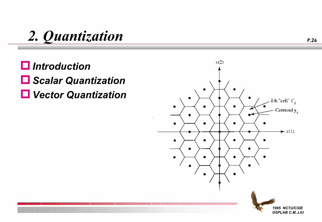
P.262. Quantization
IntroductionScalar QuantizationVector Quantization
1995 NCTU/CSIE DSPLAB C.M..LIU
P.272.1 Introduction
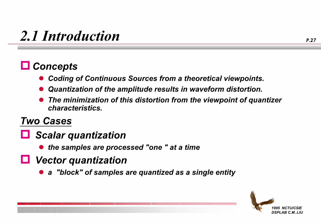
ConceptsCoding of Continuous Sources from a theoretical viewpoints.Quantization of the amplitude results in waveform distortion.The minimization of this distortion from the viewpoint of quantizer characteristics.
Two CasesScalar quantization
the samples are processed "one " at a time
Vector quantization a "block" of samples are quantized as a single entity
1995 NCTU/CSIE DSPLAB C.M..LIU
P.282.2 Scalar Quantization
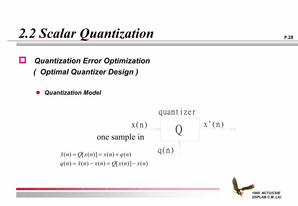
Quantization Error Optimization ( Optimal Quantizer Design )
Quantization Model
Q
quantizer
x(n)
q(n)
x'(n)
%( ) [ ( )] ( ) ( )( ) %( ) ( ) [ ( )] ( )x n Q x n x n q nq n x n x n Q x n x n
= = += − = −
one sample in
1995 NCTU/CSIE DSPLAB C.M..LIU
P.292.2 Scalar Quantization (c.1)
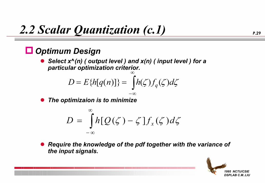
Optimum DesignSelect x^(n) ( output level ) and x(n) ( input level ) for a particular optimization criterior.
The optimizaion is to minimize
Require the knowledge of the pdf together with the variance of the input signals.
D E h q n h f dq= =−∞
∞
∫{ [ ( )]} ( ) ( )ζ ζ ζ
D h Q f dx= −− ∞
∞
∫ [ ( ) ] ( )ζ ζ ζ ζ
1995 NCTU/CSIE DSPLAB C.M..LIU
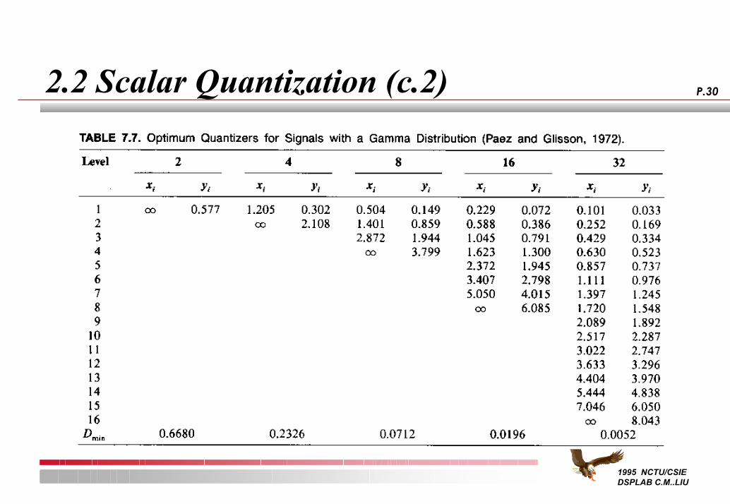
P.302.2 Scalar Quantization (c.2)
1995 NCTU/CSIE DSPLAB C.M..LIU
P.312.3 Vector Quantization
Definition
x x x x Ny y y y Nx i y i i Nx y
RN
==
≤ ≤
[ ( ) ( ) ( )][ ( ) ( ) ( )]
( ) ( )
1 21 2
1
.......... ..........
, , : real random variables , : N- dimensional random vector
the vector y has a special distribution in that it may only
take one of L ( deterministic ) vector values in
1995 NCTU/CSIE DSPLAB C.M..LIU
P.322.3 Vector Quantization (c.1)
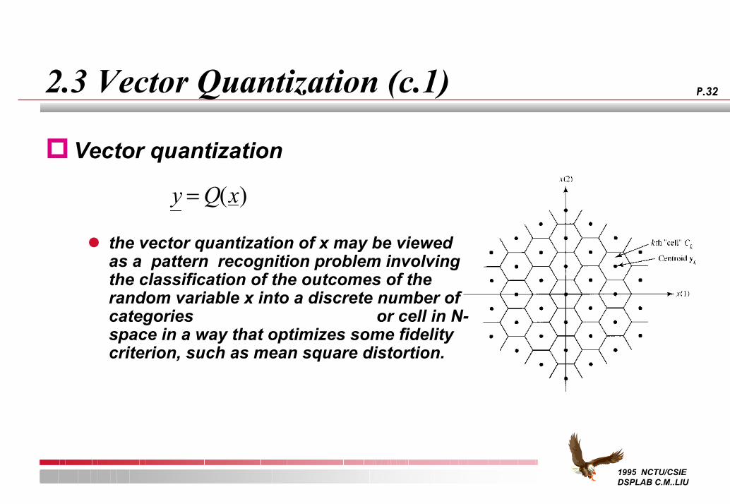
Vector quantization
the vector quantization of x may be viewed as a pattern recognition problem involving the classification of the outcomes of the random variable x into a discrete number of categories or cell in N-space in a way that optimizes some fidelity criterion, such as mean square distortion.
y Q x= ( )
1995 NCTU/CSIE DSPLAB C.M..LIU
P.332.3 Vector Quantization (c.2)
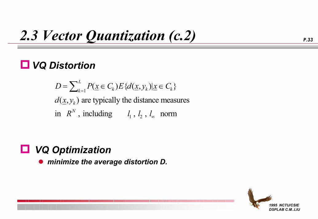
D P x C E d x y x C
d x yR l l l
k k kk
L
kN
= ∈ ∈=
∞
∑ ( ) { ( , )| }
( , )1
1 2
are typically the distance measures in , including , , norm
VQ Distortion
VQ Optimizationminimize the average distortion D.
1995 NCTU/CSIE DSPLAB C.M..LIU
P.342.3 Vector Quantization (c.3)
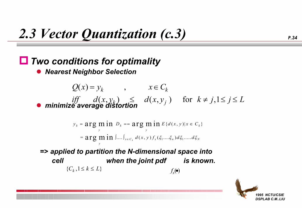
Two conditions for optimalityNearest Neighbor Selection
minimize average distortion
=> applied to partition the N-dimensional space into cell when the joint pdf is known.
Q x y x Ciff d x y d x y k j j L
k k
k j
( )( , ) ( , ,
= ∈≤ ≠ ≤ ≤
, ) for 1
y D E d x y x C
d x y f d d
ky
ky
k
yx C x n Nk
= == ∈
∫ ∫ ∈
arg m in arg m in
arg m in
{ ( , )| }
.... ( , ) ( .... ) .....
= ξ ξ ξ ξ1 1
{ , }C k Lk 1≤ ≤ fx( )•
1995 NCTU/CSIE DSPLAB C.M..LIU
P.353 Rate-Distortion Functions
IntroductionRate-Distortion Function for a Gaussian Source Rate-Distortion BoundsDistortion Measure Methods
1995 NCTU/CSIE DSPLAB C.M..LIU
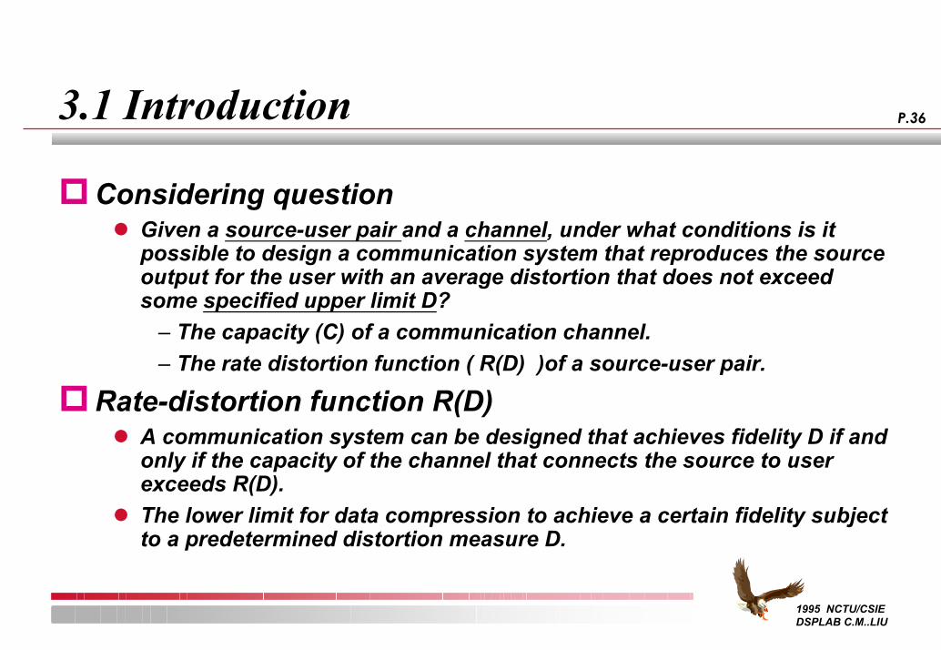
P.363.1 Introduction
Considering questionGiven a source-user pair and a channel, under what conditions is it possible to design a communication system that reproduces the source output for the user with an average distortion that does not exceed some specified upper limit D?– The capacity (C) of a communication channel. – The rate distortion function ( R(D) )of a source-user pair.
Rate-distortion function R(D)A communication system can be designed that achieves fidelity D if and only if the capacity of the channel that connects the source to user exceeds R(D).The lower limit for data compression to achieve a certain fidelity subject to a predetermined distortion measure D.
1995 NCTU/CSIE DSPLAB C.M..LIU
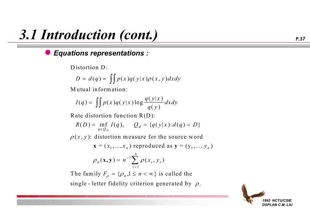
P.373.1 Introduction (cont.)Equations representations :
Distortion D :
M utual inform ation:
Rate distortion function R(D):
distortion m easure for the source word = (
D d q p x q y x x y dxdy
I q p x q y xq y xq y
dxdy
R D I q Q q y x d q D
x yx
q Q dD
= =
=
= = =
∫∫
∫∫
∈
( ) ( ) ( | ) ( , )
( ) ( ) ( | ) log( | )( )
( ) inf ( ), { ( | ): ( ) }
( , ):, ...
ρ
ρx 1 , ) , ..., )
( ) ( , )
{ , }
x y
n x y
F n
n n
t tt
n
n
reproduced as = (y
The fam ily is called the
single - letter fidelity criterion generated by .
1
n
y
x, yρ ρ
ρ
ρρ
=
= ≤ < ∞
−
=∑1
1
1
1995 NCTU/CSIE DSPLAB C.M..LIU
P.383.2 Rate-Distortion Bounds
IntroductionRate-Distortion Function for A Gaussian Source
R(D) for a memoryless Gaussian sourceSource coding with a distortion measure
Rate-Distortion BoundsConclusions
1995 NCTU/CSIE DSPLAB C.M..LIU
P.39
3.3 Rate-Distortion Function for A GaussianSource
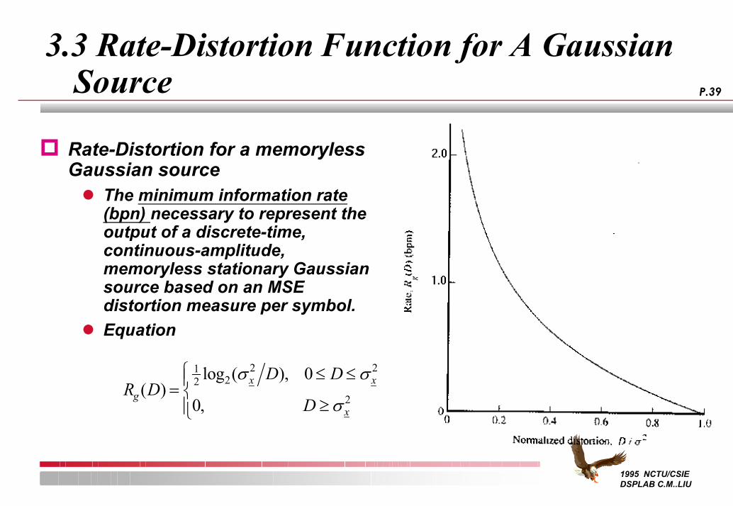
Rate-Distortion for a memoryless Gaussian source
The minimum information rate(bpn) necessary to represent the output of a discrete-time, continuous-amplitude,memoryless stationary Gaussiansource based on an MSE distortion measure per symbol.Equation
R DD D
Dgx x
x
( )log ( ),
,=
≤ ≤
≥
12 2
2 2
2
0
0
σ σ
σ
1995 NCTU/CSIE DSPLAB C.M..LIU
P.40
3.3 Rate-Distortion Function for A GaussianSource (c.1)
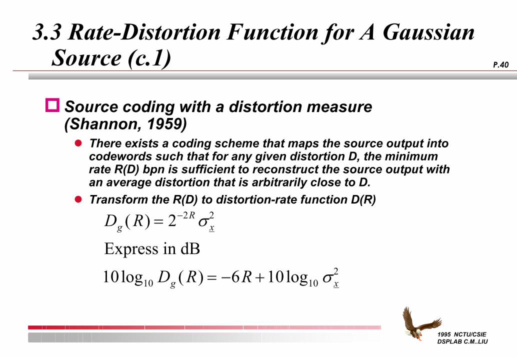
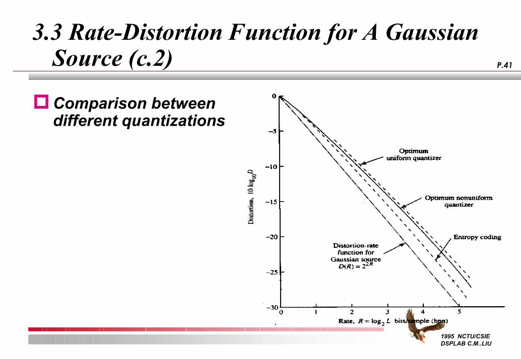
Source coding with a distortion measure (Shannon, 1959)
There exists a coding scheme that maps the source output intocodewords such that for any given distortion D, the minimum rate R(D) bpn is sufficient to reconstruct the source output with an average distortion that is arbitrarily close to D.Transform the R(D) to distortion-rate function D(R)
D R
D R R
gR
x
g x
( )
log ( ) log
=
= − +
−2
10 6 10
2 2
10 102
σ
σ
Express in dB
1995 NCTU/CSIE DSPLAB C.M..LIU
P.41
3.3 Rate-Distortion Function for A GaussianSource (c.2)
Comparison between different quantizations
1995 NCTU/CSIE DSPLAB C.M..LIU
P.423.4 Rate-Distortion Bounds
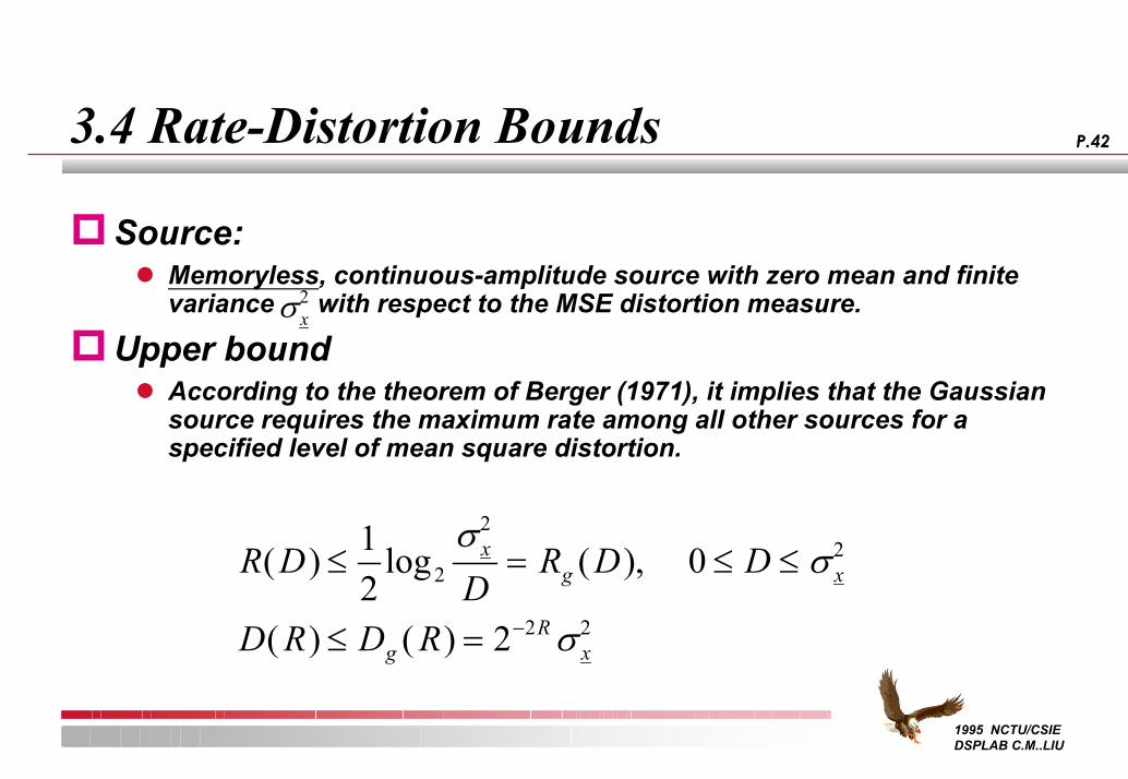
Source:Memoryless, continuous-amplitude source with zero mean and finite variance with respect to the MSE distortion measure.
Upper boundAccording to the theorem of Berger (1971), it implies that the Gaussiansource requires the maximum rate among all other sources for a specified level of mean square distortion.
R DD
R D D
D R D R
xg x
gR
x
( ) log ( ),
( ) ( )
≤ = ≤ ≤
≤ = −
12
0
2
2
22
2 2
σσ
σ
σx2
1995 NCTU/CSIE DSPLAB C.M..LIU
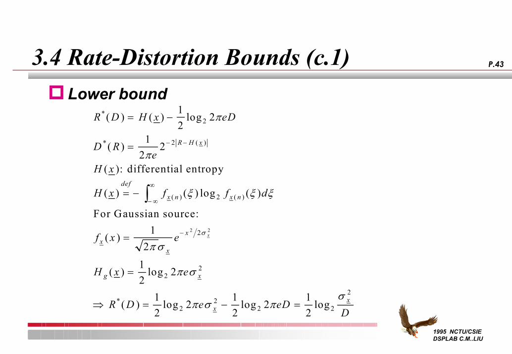
P.433.4 Rate-Distortion Bounds (c.1)Lower bound
R D H x eD
D Re
H x
H x f f d
f x e
H x e
R D e
R H x
def
x n x n
xx
x
g x
x
*
* ( )
( ) ( )
*
( ) ( ) log
( )
( ):
( ) ( ) log ( )
( )
( ) log
( ) log
= −
=
= −
=
=
⇒ =
− −
−∞
∞
−
∫
12
2
12
2
12
12
2
12
2
2
2
2
2
22
2
2 2
π
π
ξ ξ ξ
π σ
π σ
π
σ
differential entropy
For Gaussian source:
σ πσ
xxeDD
22 2
212
212
− =log log
1995 NCTU/CSIE DSPLAB C.M..LIU
P.443.4 Rate-Distortion Bounds (c.2)
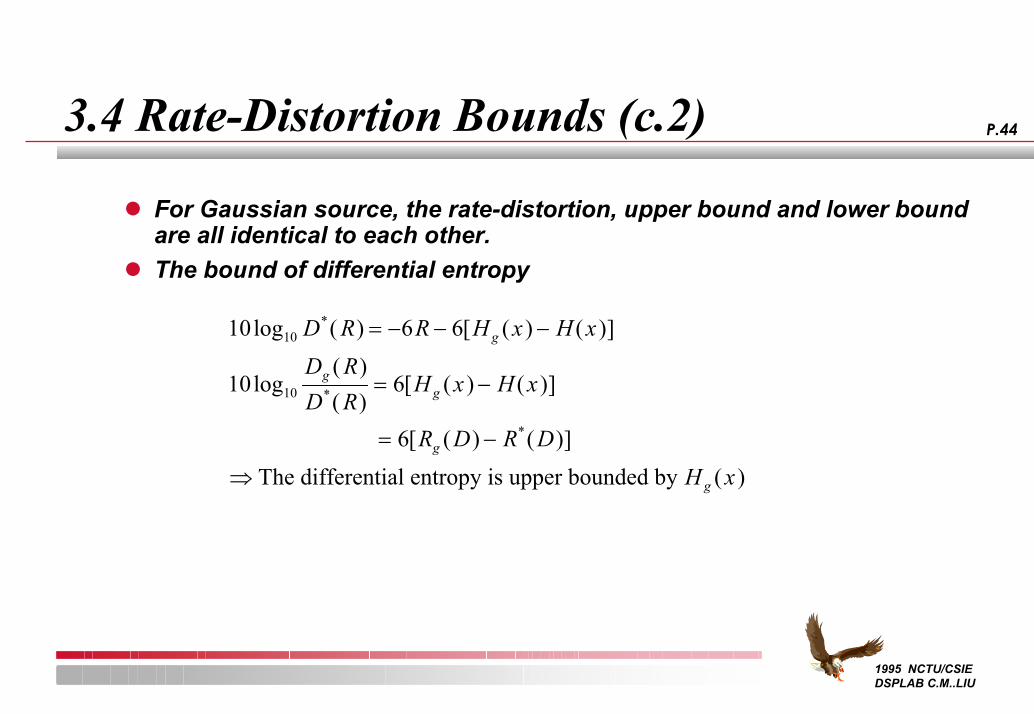
For Gaussian source, the rate-distortion, upper bound and lower bound are all identical to each other.The bound of differential entropy
10 6 6
10 6
6
10
10
log ( ) [ ( ) ( )]
log( )( )
[ ( ) ( )]
[ ( ) ( )]( )
*
*
*
D R R H x H xD RD R
H x H x
R D R DH x
g
gg
g
g
= − − −
= −
= −
⇒
The differential entropy is upper bounded by
1995 NCTU/CSIE DSPLAB C.M..LIU
P.453.4 Rate-Distortion Bounds (c.3)
Rate-distortion R(D) to channel capacity CFor C > Rg(D) – The fidelity (D) can be achieved.
For R(D)<C< Rg(D) – Achieve fidelity for stationary source– May not achieve fidelity for random source
For C<R(D)– Can not be sure to achieve fidelity
1995 NCTU/CSIE DSPLAB C.M..LIU
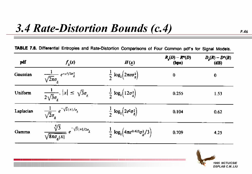
P.463.4 Rate-Distortion Bounds (c.4)
1995 NCTU/CSIE DSPLAB C.M..LIU
P.473.5 Distortion Measure Methods
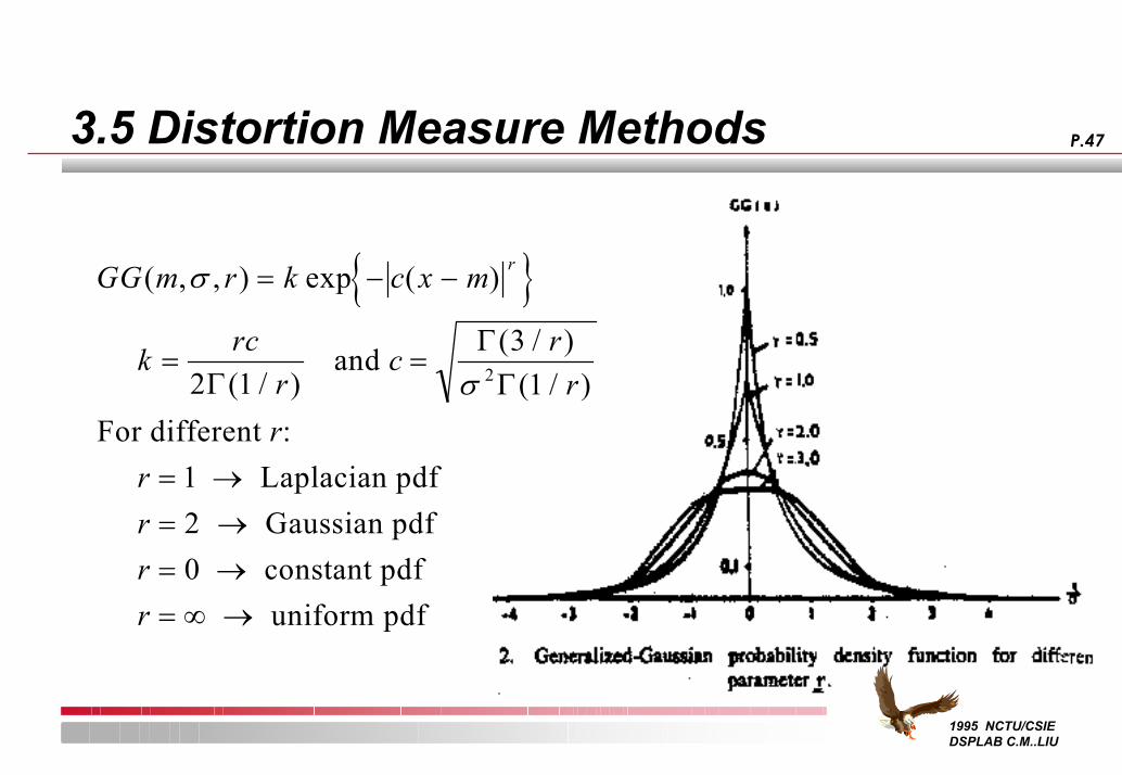
{ }GG m r k c x m
k rcr
c rr
rrrrr
r( , , ) exp ( )
( / )( / )
( / ):
σ
σ
= − −
= =
= →= →= →= ∞ →
and
For different Laplacian pdf Gaussian pdf constant pdf uniform pdf
2 13
1
120
2ΓΓΓ
1995 NCTU/CSIE DSPLAB C.M..LIU
P.484. Waveform Coding
IntroductionPulse Code Modulation(PCM)Log-PCMDifferential PCMAdaptive DPCM
1995 NCTU/CSIE DSPLAB C.M..LIU
P.494.1 Introduction
Two SCoding Categories 1 . Waveform coder2 . Perceptual coder
Waveform Coding Methods for digitally representing the temporal or spectral characteristics of waveforms.
VocodersParametric Coders, the parameters characterize the short-term spectrum of a sound.These parameters specify a mathematical model of human speech production suited to a particular sound.
1995 NCTU/CSIE DSPLAB C.M..LIU
P.504.2 Pulse Code Modulation
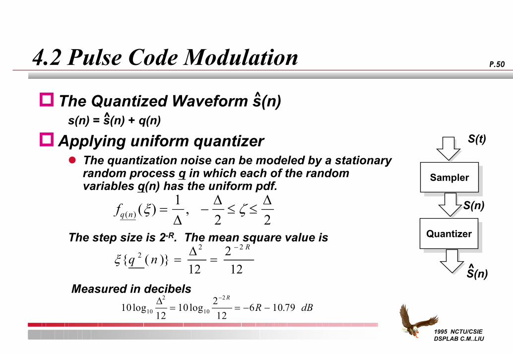
The Quantized Waveform s(n)s(n) = s(n) + q(n)
Applying uniform quantizerThe quantization noise can be modeled by a stationary random process q in which each of the random variables q(n) has the uniform pdf.
The step size is 2-R. The mean square value is
Measured in decibels
^
1012
10 212
6 10 7910
2
10
2
log log .∆= = − −
− R
R dB
^
fq n( ) ( ) ,ξ ζ= − ≤ ≤1
2 2∆∆ ∆
ξ{ ( )}q nR
22 2
12212
= =−∆
SamplerSampler
S(t)
QuantizerQuantizer
S(n)
S(n)^
1995 NCTU/CSIE DSPLAB C.M..LIU
P.514.3 Log PCM
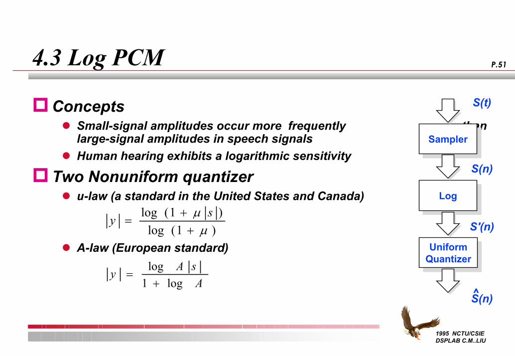
ConceptsSmall-signal amplitudes occur more frequently than large-signal amplitudes in speech signalsHuman hearing exhibits a logarithmic sensitivity
Two Nonuniform quantizeru-law (a standard in the United States and Canada)
A-law (European standard)
SamplerSampler
S(t)
LogLog
S(n)
S(n)^
Uniform QuantizerUniform
Quantizer
S'(n)y s=
++
log ( )log ( )
11
µµ
y A sA
=+
loglog1
1995 NCTU/CSIE DSPLAB C.M..LIU
P.524.3 Log PCM(c.1)
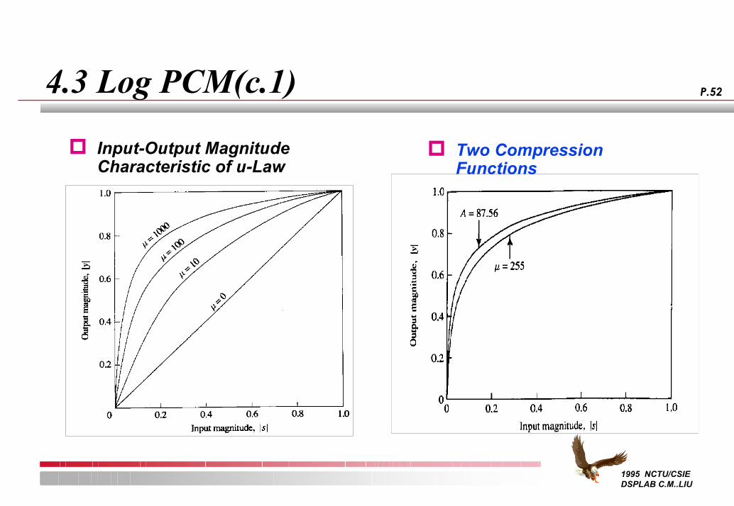
Input-Output Magnitude Characteristic of u-Law
Two Compression Functions
1995 NCTU/CSIE DSPLAB C.M..LIU
P.534.4 Differential PCM (DPCM)
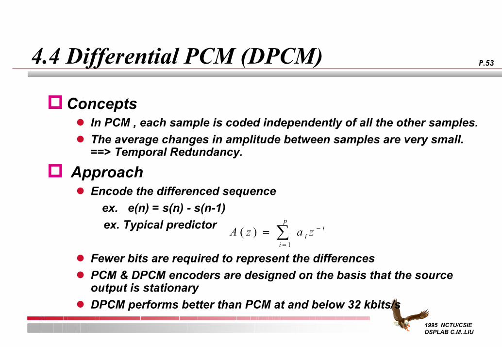
ConceptsIn PCM , each sample is coded independently of all the other samples.The average changes in amplitude between samples are very small.==> Temporal Redundancy.
ApproachEncode the differenced sequence
ex. e(n) = s(n) - s(n-1) ex. Typical predictor
Fewer bits are required to represent the differencesPCM & DPCM encoders are designed on the basis that the source output is stationary DPCM performs better than PCM at and below 32 kbits/s
A z a zii
i
p
( ) = −
=∑
1
1995 NCTU/CSIE DSPLAB C.M..LIU
P.544.4 Differential PCM (c.1)
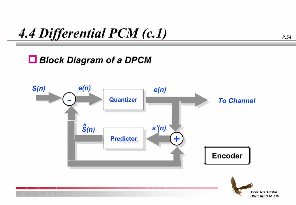
Block Diagram of a DPCM
Quantizer
S(n)^
--
++
e(n)S(n) e(n)Quantizer To Channel
s'(n)
PredictorPredictor
Encoder
1995 NCTU/CSIE DSPLAB C.M..LIU
P.564.5 Adaptive DPCM
ConsiderationsSpeech signals are quasi-stationary in natual
ConceptsAdapt to the slowly time-variant statistics of the speech signal Adaptive quantizer is usedFeedforward and feedback adaptive quantizer.
Examplelooks at only one previosly quantized sample and either expands or compresses the quantizer intervals.
∆ ∆n n iM x+ =1 ( ))
1995 NCTU/CSIE DSPLAB C.M..LIU
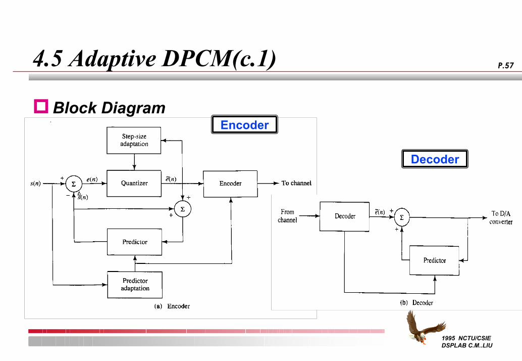
P.574.5 Adaptive DPCM(c.1)
EncoderBlock Diagram
Decoder
1995 NCTU/CSIE DSPLAB C.M..LIU
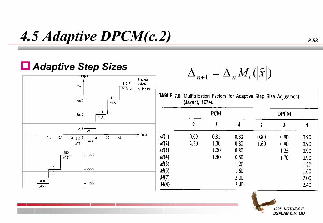
P.584.5 Adaptive DPCM(c.2)
∆ ∆n n iM x+ =1 ( ))Adaptive Step Sizes
1995 NCTU/CSIE DSPLAB C.M..LIU
P.594.5 Adaptive DPCM(c.3)
CCITT G.721 standard (1988)Adaptive quantizer – quantize e(n) into 4 bits words.
Adaptive predictor– Pole-zero predictor with 2 poles, 6 zeros.– Coefficients are estimated using a gradient algorithm and the
stability is checked by testing two roots of A(z).The performance of the coder in terms of MOS is above 4.The G.721 ADPCM algorithm was modified to accomodate 24 and 40kbits/s in G.723.The performance of ADPCM degrades quickly for rates below 24 kbits/s.
1995 NCTU/CSIE DSPLAB C.M..LIU
P.604.6 Summary
IntroductionPulse Code Modulation(PCM)Log-PCMDifferential PCMAdaptive DPCM
1995 NCTU/CSIE DSPLAB C.M..LIU
P.615. Subband Coding
ConceptsExploits the redundancy of the signal in the frequency domain.Quadrature-Mirror Filter for subband coding.The opportunitylies in both the short-time power spectrum and the the perceptual properties of the human ear.
StandardsAT&T voice store-and-forward standard.– 16 or 24 kbits/s– Five-band nonuniform tree-structured QMF band in conjunction
with ADPCM coders– The frequecy range for each band are 0-0.5, 0.5-1, 1-2, 2-3, 3-4
kHz.– {4/4/2/2/0} for 16 kbits and {5/5/4/3/0} for 24 kbits.– The one-way delay is less than 18 ms.
1995 NCTU/CSIE DSPLAB C.M..LIU
P.625. Subband Coding (c.1)
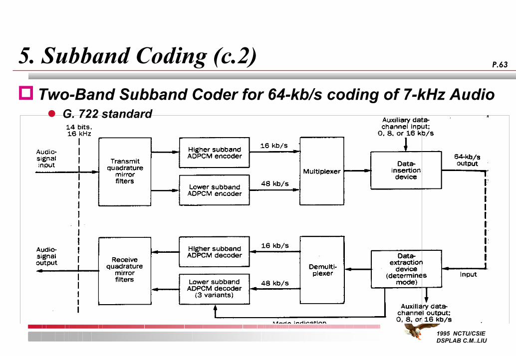
CCITT G.722G. 722 algorithm at 64 kb/s have an equivalent SNR gain of 13 db over the G.721.Low-frequency parts permit operation at 6, 5, or 4 bits (64, 56, and 48 kb/s) per sample with graceful degradation of quality.Two-band subband coder with ADPCM coding of each subband.The low- and high-frequency subbands are quantized using 6 and 2 bits per sample, respectively.The filter banks produce a communication delay of about 3 ms.The MOS at 64 kbits/s is greater than 4 for music signals.
1995 NCTU/CSIE DSPLAB C.M..LIU
P.635. Subband Coding (c.2)Two-Band Subband Coder for 64-kb/s coding of 7-kHz Audio
G. 722 standard
1995 NCTU/CSIE DSPLAB C.M..LIU
P.646. Transform Coding
ConceptsThe transform components of a unitary transform are quantized at the transmitter and decoded and inver-transformed at receiver.
Unitary transformsKarhunen-Loeve Transform– Optimal in the sense that the transform components are maximally
decorrelated for any given signal.– Data dependent.
The Discrete Cosine Transform– Near optimal.
The Fast Fourier Transform– Approaches that of DCT for very large block.


![course.ece.cmu.eduece796/documents/MPEG-1... · Web viewMS stereo [audio]: A method of exploiting stereo irrelevance or redundancy in stereophonic audio programmes based on coding](https://img.pdfslide.us/doc/110x75/60cebdf0d6e288136150cf52/ece796documentsmpeg-1-web-view-ms-stereo-audio-a-method-of-exploiting.jpg)