Attitudes towards Uncertainty and Randomization: An ... · (1987) and Sarin and Wakker (1992). 2 See Ghirardato (1997) and Klibano (2001) for theoretical contributions on the role

U n i v e r s i t y o f H e i d e l b e r g

Department of Economics

Discussion Paper Series No. 494

Attitudes towards Uncertainty and Randomization: An Experimental Study

Adam Dominiak and Wendelin Schnedler

December 2009

Attitudes towards Uncertainty

and Randomization:

An Experimental Study

Adam Dominiak∗


University of Heidelberg

Wendelin Schnedler∗∗


University of Heidelberg

December 21, 2009

Abstract

Individuals exhibit a randomization preference if they prefer random mix-

tures of two bets to each of the involved bets. Such preferences provide the

foundation of various models of uncertainty aversion. However, it has to our

knowledge not been empirically investigated whether uncertainty-averse deci-

sion makers indeed exhibit such preferences. Here, we examine the relationship

experimentally. We �nd that uncertainty aversion is not positively associated

with randomization preferences. Moreover, we observe choices that are not

consistent with the prevailing theories of uncertainty aversion: a non-negligible

number of uncertain-averse subjects seem to dislike randomization.

Keywords: uncertainty aversion, randomization preference, ambiguity, Choquet ex-pected utility model, maxmin expected utility model, experiment

JEL-Codes: D8, C9

∗[email protected]∗∗[email protected], University of Heidelberg, Department of Eco-

nomics, Bergheimer Straÿe 58, D-69115 Heidelberg, Germany. The authors wish to thank JürgenEichberger, Simont Grant, David Kelsey, Jean-Philippe Lefort, Jörg Oechssler, Arno Riedl andDavid Schmeidler for their valuable comments.Financial support from the Deutsche Forschungsgemeinschaft, SFB 504, is gratefully acknowledged.

1 Introduction

The canonical paradigm for economists to model choice behavior under uncertainty

is that of subjective expected utility theory (Savage, 1954; Anscombe and Aumann,

1963). Ellsberg (1961) challenged this paradigm by suggesting a series of experi-

ments. Consider, for example, two urns that are �lled with yellow and white balls.

In one urn, half of the balls are yellow, the other white. In the other urn, the

proportion of yellow and white balls is unknown. A ball is drawn and subjects re-

ceive 100 if they guess the color correctly, and nothing otherwise. Many subjects

are indi�erent between yellow and white but prefer betting on the urn with known

proportions (urn K) to betting on the urn with unknown proportions (urn U). They

are uncertainty-averse and their choices violate subjective expected utility theory;

moreover, their behavior is not consistent with probabilistic sophistication in the

sense of Machina and Schmeidler (1992).

In a direct comment on Ellsberg's thought experiment Rai�a (1961) suggested

the following. After drawing a ball from urn U, subjects �ip a fair coin to decide

on which color to bet. By tossing a fair coin and betting on yellow when heads

appear and on white otherwise, the objective chances of winning the bet are 50%

and thus identical to those when betting on urn K. This seems to contradict the idea

that betting on urn K is preferable to betting on urn U. Indeed, Rai�a proposes the

randomization to `undermine the con�dence' of uncertainty-averse subjects in their

choices. However, subjects who value bets on urn K and randomized bets on urn U

equally may still exhibit uncertainty aversion, if they prefer a coin toss to determine

the color of the winning ball rather than betting on either white or yellow when

they face uncertainty. In short, subjects may agree with Rai�a's argument and still

be uncertainty-averse if they have a randomization preference.

In view of the overwhelming empirical evidence pointing to uncertainty aver-

sion (see the survey article by Camerer and Weber, 1992), various alternatives to

subjective expected utility theory have been proposed. Many of these alternative

1

theories, including Schmeidler's (1989) Choquet expected utility model with convex

capacities, the multiple prior model of Gilboa and Schmeidler (1989), the smooth

second-order prior model of Klibano�, Marinacci, and Mukerji (2005) and the vari-

ational preferences model of Maccheroni, Marinacci, and Rustichini (2006), adopt

the idea of randomization preferences to formally model uncertainty aversion. Cur-

rently, there is a theoretical debate whether uncertainty-averse subjects exhibit ran-

domization preferences�see Epstein (2009) and Klibano�, Marinacci, and Mukerji

(2009). Moreover, predicting equilibria in games depends on whether uncertainty-

averse players prefer randomization (Klibano� 1996 and Lo 1996), or not (Dow and

Werlang 1994, Eichberger and Kelsey 2000, and Marinacci 2000). However, it has

to our knowledge not been empirically investigated whether uncertainty-averse sub-

jects prefer randomization. We examine the relationship between di�erent attitudes

towards uncertainty and randomization in an experimental study.

Subjects in the experiment were faced with three random devices: a coin, an urn

with a known proportion of yellow and white balls, and an urn with an unknown pro-

portion. We o�ered bets based on these devices (called tickets) and elicited subjects'

valuations for these tickets. We then classify subjects by their uncertainty attitude.

The de�nition that we use captures the intuition that an uncertainty-averse sub-

ject values otherwise identical bets more if they are based on urn K rather than

urn U. It coincides with the general de�nition proposed by Epstein (1999). Ran-

domization attitude is measured using a ticket that mimics Rai�a's idea and which

we call chameleon ticket. This chameleon ticket involves deliberate randomization

between betting on white and on yellow when facing urn U. A subject who prefers

the chameleon ticket to betting on urn U is classi�ed as randomization-loving. The

employed notions of uncertainty and randomization attitude are independent of each

other and are hence suited to empirically study the relationship between uncertainty

aversion and randomization preference without foreclosing results.

Existing theories restrict the relationship between uncertainty and randomization

2

attitude in several ways that we can directly test with our experimental setup. First,

the notion of mixture over bets embodied in Schmeidler's de�nition of uncertainty

aversion coincides with our de�nition of randomization loving for subjects who are

indi�erent between betting on yellow and white given urn U. This notion, which is

at the heart of uncertainty aversion in various models, suggests our �rst hypothe-

sis: randomization and uncertainty attitude are negatively related, i.e., uncertainty

aversion is associated with randomization-loving preferences.

Second, and somewhat more speci�cally, the most prominent approach to model

uncertainty aversion is the Choquet expected utility model with convex capacities.

Depending on how the randomization device is modeled, this theory leads to di�er-

ent predictions with respect to randomization attitudes. The more popular way is

to model the device in the tradition of Anscombe and Aumann (1963) as part of

the consequence space (C-approach). For this approach, Schmeidler (1989) proves

that decision makers with convex capacities are always randomization-loving. On

the other hand, the randomization device can also be modeled à la Savage (1954)

by extending the state space (S-approach).1 For the S-approach, Eichberger and

Kelsey (1996) show that decision makers with convex capacities are randomization-

neutral.2 These two diverging predictions yield the second hypothesis: subjects

who are indi�erent between betting on white and yellow when facing urn U are

randomization-loving (C-approach) or randomization-neutral (S-approach).

The main �nding is that uncertainty and randomization attitude seem to be

unrelated; the hypothesis that they are independent cannot be rejected at any con-

ventional level. If anything, association measures suggest that uncertainty-averse

subjects are randomization-averse rather than loving. This �nding questions that

1Choquet expected utility preferences in the Savage (1954) setting were axiomatized by Gilboa

(1987) and Sarin and Wakker (1992).

2See Ghirardato (1997) and Klibano� (2001) for theoretical contributions on the role of ran-

domization for Choquet expected utility preferences with convex capacities.

3

the notion of randomization preference underpins uncertainty aversion.

The second �nding is that uncertainty-averse subjects who are indi�erent be-

tween betting on white and yellow when facing urn U are more likely to be randomi-

zation-neutral rather than loving. The S-approach thus �ts our data better than

the C-approach.

Both hypotheses apply by construction only to subjects who exhibit speci�c

preferences. Being concerned about selection e�ects, we check for selection on ob-

servables and re-examine results on the full sample. There is no indication for

selection and the two �ndings are robust.

The rest of the paper is organized as follows. The next section describes the

experimental design. In Section 3, we derive our hypotheses. Section 4 presents the

results. The article ends with some concluding remarks.

2 Experimental design

In order to examine the relationship between uncertainty and randomization at-

titude, information about both attitudes from the same subject is required. We

elicited the value of various bets, which are based on three random devices. This

section describes the random devices, the bets, and the elicitation mechanism.

2.1 Random devices

During the experiment, we used three di�erent random devices: an urn with 20

table tennis balls of which half were white and the other half yellow (urn with

known proportions or short: urn K), an urn with 20 table tennis balls with an

unknown proportion of yellow and white balls (short: urn U), and a coin.

Subjects were informed that only white and yellow balls are used in the exper-

iment. Urn K's contents were shown to the subjects before the experiment, while

urn U's contents were only revealed after the experiment. During the experiment,

4

both urns were placed on a table in view of the subjects to convince them that their

contents were not manipulated. For similar reasons, the coin was volunteered by

one of the subjects and not by us.

Tickets

While subjects knew that they would be o�ered di�erent bets involving the three

random devices, they did not know which or how many bets they would face. Tickets

were then presented and evaluated by the subjects in the following order. In the

description of the tickets, as in the experiment, outcomes are expressed in Taler, our

experimental currency unit.

In order to check whether subjects regard the coin as fair, we introduced the

following tickets.

1. Head ticket, h: 100 Taler are paid if the coin lands heads up and nothing

otherwise.

2. Tails ticket, t: 100 Taler are paid if the coin lands tails up and nothing

otherwise.

To elicit uncertainty attitude, we ask the subjects to evaluate the following tickets

for urn K.

3. White ticket for urn K, wK : 100 Taler are paid if the drawn ball from

urn K is white and nothing otherwise.

4. Yellow ticket for urn K, yK , 100 Taler are paid if the drawn ball from urn

K is yellow and nothing otherwise.

Uncertainty attitude is then detected by comparing the value of these tickets with

that of the following similar tickets for urn U.

5. Yellow ticket for urn U, yU : 100 Taler are paid if the drawn ball from urn

U is yellow and nothing otherwise.

5

6. White ticket for urn U, wU : 100 Taler are paid if the drawn ball from urn

U is white and nothing otherwise.

The next ticket was designed in the spirit of Rai�a's idea. It involves two random

devices: the coin and urn U. The subject always receives a ticket for urn U. Whether

this ticket will be yellow or white is determined by �ipping the coin. Since the color

of the ticket changes with the outcome of the coin toss, we use the name chameleon

ticket.

7. Chameleon ticket for urn U, cU : If the coin lands heads up, the subject

receives a yellow ticket for urn U. If the coin lands tails up the subject receives

a white ticket for urn U.3

By comparing the certainty equivalent for the chameleon ticket with that of a yellow

or white ticket for urn U, we can draw some inference about a subject's randomiza-

tion preference.

For our predictions later, it must be possible to identify whether subjects are

indi�erent between yellow and white tickets on urn U. This necessitates that sub-

jects are asked about both tickets, which in principle allows them to hedge against

uncertainty. The danger of hedging against uncertainty is that subjects no longer

exhibit uncertainty aversion. We tried to reduce this danger by not informing sub-

jects about the number and types of bets and switching the order in which tickets are

presented for urn U. Consequently, subjects do not know that there will be a hedg-

ing opportunity when evaluating the yellow ticket for urn U. As we will see later,

our method was successful in the sense that the proportion of uncertainty-averse

subjects in our experiment is in line with that of similar experiments.

3Put di�erently, the subject receives 100 Taler in two cases: if the coin lands heads up and the

drawn ball from urn U is yellow and if the coin lands tails up and the ball drawn from urn U is

white. In the other two cases, the subject receives nothing.

6

Eliciting ticket values

In order to elicit ticket values, we used the following procedure. For each ticket, the

subject had to make twenty choices. The �rst choice was between a ticket and a

payment of 2.5 Taler. The second was between a ticket and a payment of 7.5 Taler

etc. The payments o�ered to the subject increased in steps of 5 Taler until the last

choice, in which the subject had to choose between a ticket and 97.5 Taler. The

point at which the subject switches from the ticket to the payment then reveals the

value of the ticket to the subject (up to 5 Taler). All of the subject's choices were

implemented and a�ected the subject's payo�. To ensure independence, a separate

draw was carried out for each ticket. The draws took place after all choices were

made to avoid wealth e�ects.

Many experiments employ less time-consuming and laborious elicitation mech-

anisms that combine the choices over bets with additional randomization. For ex-

ample, Holt and Laury (2002) propose to randomly select only one of many choices

to be payo� relevant. Another popular mechanism, which has been used in experi-

ments on uncertainty aversion (Halevy, 2007; Hey, Lotito, and Ma�oletti, 2008), is

that of Becker, DeGroot, and Marschak (1964). In the Becker-DeGroot-Marschak

mechanism, the subject receives a ticket and states the certainty equivalent. Then,

a random o�er is generated and the subject has to sell the ticket if the o�er exceeds

the stated value.

Despite the considerable e�ort involved, we decided to pay all decisions rather

than employing a mechanism that relies on additional randomization. We do so

for two reasons. First, as Karni and Safra (1987) point out a method based on

additional randomization, such as the Becker-DeGroot-Marschak mechanism, is no

longer guaranteed to elicit the true (subjective) value for subjects who violate the

independence axiom.4 Since uncertainty-averse subjects violate the independence

4A similar observation has been made by Holt (1986). The Becker-DeGroot-Marschak mecha-

nism also fails to elicit true valuations if the compound lottery axiom is violated (Segal, 1988).

7

axiom and we are interested in their valuations, we cannot use this mechanism.5

Second, had we introduced another source of randomness, all bets faced by the

subject would have been compounded; none would have been purely based on the

three devices that we are interested in (coin, urn K, urn U). By implementing all

choices, we avoid that randomization preferences interact with other sources of ran-

domness.

3 Uncertainty and randomization attitude

In this section, we de�ne randomization and uncertainty attitude, relate them to

concepts from the literature, and derive empirical predictions. Let L be the set

of tickets faced by subjects in our experiment. The binary relation < represents

subjects preferences over L. Denote by µ(l) a subject's certainty equivalent or value

of ticket l in L. For any two tickets k and l in L, we say that subjects weakly prefer

k to l, written k < l, if and only if µ(k) > µ(l).

3.1 De�nitions

Comparing the certainty equivalents for the white and yellow ticket for urn U with

that for the chameleon ticket, we can classify subjects according to their random-

ization attitudes. Consider a subject who favours the yellow ticket yU to the white

ticket wU for urn U , i.e., yU < wU . Such a subject is randomization-averse if

she values the chameleon ticket even less than the white ticket wU . Conversely,

such a subject is randomization-loving if she values the chameleon ticket even more

than the yellow ticket yU . If a subject values the chameleon ticket weakly more

than the white ticket wU but weakly less than the yellow ticket wU , we say she is

5Apart from the theoretical argument, there is empirical evidence that preference rever-

sals in measurements of uncertainty aversion occur when using the Becker-DeGroot-Marschak

mechanism�see Trautmann, Vieider, and Wakker (2009).

8

randomization-neutral. The next de�nition formalizes this idea, where sU and tU

stands for the favorite and least favorite ticket on urn U.

De�nition 1 (Randomization attitude). A subject with sU < tU , where sU , tU ∈

{yU , wU}, is: (i) randomization-averse if sU < tU � cU ,

(ii) randomization-neutral if sU < cU < tU ,

(iii) randomization-loving if cU � sU < tU .

As will become clear later, this de�nition coincides with the idea of a preference for

convex combinations embodied in Schmeidler's (1989) uncertainty aversion axiom

for subjects who are indi�erent between the yellow and white ticket on urn U.

Subjects are typically regarded to be uncertainty-averse if they prefer betting on

the urn with known proportions of yellow and white balls. Let us be more precise

about this statement by considering a subject who weakly prefers the yellow to the

white ticket on both urns (yK < wK and yU < wU). Suppose this subject compares

her two favorite tickets (yK and yU) and her two least favorite tickets (wK and wU)

across urn K and urn U. Then this subject is uncertainty-averse if she weakly prefers

the tickets on urn K to those on urn U for her favorite as well as least favorite tickets

and her preference is strict in at least one case: yK < yU and wK < wU with at least

one strict preference (�). Conversely, she is uncertainty-loving if she weakly prefers

the tickets based on urn U in both cases and strictly in at least one case: yU 4 yK

and wU 4 wK with at least one strict preference (≺). Finally, she is uncertainty-

neutral if she either prefers another urn for her favorite tickets than for her least

favorite tickets or if she is indi�erent between urns for the favorite as well as least

favorite tickets: yU � yK but wK ≺ wU , or yU � yK but wK � wU , or yU ∼ yK and

wU ∼ wK . The following de�nition generalizes this idea to arbitrary preferences,

where qK and rK stands for the favorite and least favorite ticket on urn K, and sU

and tU for the favorite and least favorite ticket on urn U. The de�nition is complete

in the sense that each preference ordering is either uncertainty-averse, uncertainty-

loving, or uncertainty-neutral.

9

De�nition 2 (Uncertainty attitude). A subject with qK < rK and sU < tU ,

where qK , rK ∈ {yK , wK} and sU , tU ∈ {yU , wU}, is:

(i) uncertainty-averse if qK < sU and rK < tU with at least one (�),

(ii) uncertainty-loving if qK 4 sU and rK 4 tU with at least one (≺),

(iii) uncertainty-neutral otherwise, i.e.,

if qK ∼ sU and rK ∼ tU ,

or qK � sU and rK ≺ tU ,

or qK ≺ sU and rK � tU .

It is customary to view urns with known proportions of balls and coins as risky.

Based on exogenously given risky bets, Epstein (1999) derives a comparative foun-

dation of uncertainty attitudes. Given that bets on urn K are risky, our de�nition

coincides with that of Epstein (see appendix). Ghirardato and Marinacci (2002)

propose an alternative comparative de�nition of uncertainty aversion without ex-

ogenously imposing that certain bets are risky. For this de�nition, it is necessary to

hold the subject's risk attitude constant. Empirically, this requires measuring the

risk attitude, which in turn is not possible without exogenous assumptions about

which bets are risky. Accordingly, we cannot use this alternative approach to deter-

mine uncertainty attitude in our experiment.

3.2 Predictions

The general de�nitions allow for any combination of uncertainty and randomization

attitude. For example, a subject may in principle be uncertainty-neutral but like

randomization or it may be averse to uncertainty and randomization. This section

uses existing theoretical models to restrict the relationship between uncertainty and

randomization attitude and derive predictions.

In order to represent uncertainty aversion, a large class of models appeals to

Schmeidler's (1989) notion that a mixture between two bets is preferred to each of

10

the bets itself. In the speci�c framework used by Schmeidler, bets are mappings

from events to probability distributions over the set of payo�s, so that the convex

combination of two bets, f and g: αf + (1 − α)g with α ∈ (0, 1) is well de�ned.

Schmeidler calls a subject with f � g uncertainty-averse if

αf + (1− α)g � g.

For subjects who violate the independence axiom, the convex combination is strictly

preferred. Interpreting α as the probability of obtaining a yellow ticket for urn U

and 1− α as the probability of obtaining a white ticket for urn U, this means that

an uncertainty-averse subjects prefers the chameleon ticket, i.e., the mixture of two

bets, to the least favorite ticket on urn U. Restricting attention to subjects with

yU ∼ wU , we get: cU � wU ∼ yU . Schmeidler's notion then coincides with the

de�nition of randomization-loving (see De�nition 1). In perfect analogy, subjects

are (strict) uncertainty-loving according to Schmeidler if αf + (1− α)g ≺ f, which

means that cU ≺ wU ∼ yU for subjects with yU ∼ wU ; the dislike for mixtures then

is equivalent to randomization aversion in De�nition 1.

For subjects who are indi�erent between the yellow and white ticket for urn U,

Schmeidler's notion of preferences for mixtures thus coincides with our de�nition

of randomization attitude. Based on the various models that appeal to prefer-

ences for mixtures to explain uncertainty attitude, we hence predict uncertainty-

averse subjects to be randomization-loving and uncertainty-loving subjects to be

randomization-averse (given yU ∼ wU).

Hypothesis 1

For subjects who are indi�erent between the yellow and white ticket on urn U, yU ∼

wU , uncertainty and randomization attitude are negatively associated: uncertainty-

averse subjects are randomization-loving and vice versa.

As the null hypothesis, we consider that there is no relationship between uncertainty

11

and randomization attitude.

If uncertainty aversion is modeled using Choquet expected utility models with

convex capacities, the relationship between uncertainty and randomization attitude

depends on whether the randomization device is modeled as part of the consequence

space (C approach) or as an extension of the state space (S approach). As Eichberger

and Kelsey (1996) show that uncertainty-averse decision makers who are indi�erent

between two acts based on an uncertain urn, yU ∼ wU , and who regard the ran-

domization device as fair, h ∼ t, are randomization-loving in the C-approach but

are randomization-neutral in the S-approach. This directly leads to the hypotheses.

Hypothesis 2C

Uncertainty-averse subjects with yU ∼ wU and h ∼ t are randomization-loving.

Hypothesis 2S

Uncertainty-averse subjects with yU ∼ wU and h ∼ t are randomization-neutral.

We test these two alternatives against the null hypothesis that uncertainty-averse

subjects with yU ∼ wU and h ∼ t are equally likely to be randomization-neutral and

randomization-loving.

4 Implementation

We ran a total of 5 sessions with 90 subjects. All sessions were conducted in the

experimental laboratory at the University of Mannheim in late September 2008.

Subjects were primarily students who were randomly recruited from a pool of ap-

proximately 1000 subjects using an e-mail recruitment system. Each subject only

participated in one of the sessions. Ticket values were elicited electronically using

the software z-tree (Fischbacher, 2007).

After the subjects' arrival at the laboratory, they were randomly seated at the

12

computer terminals. Instructions were read out loud and ticket types were practi-

cally explained. Then, the subjects were given time to study the instructions (see

appendix for a translation of the instructions). Finally, they were asked to answer

a series of questions to test their understanding of the instructions. During all this

time, subjects could ask the experimenters clarifying questions. This part lasted

about 30 minutes. It was followed by the evaluation of the tickets. In order to sim-

plify the input for subjects, we programmed a slider that allowed them to specify

their value for each ticket. The program then automatically selected choices that

were consistent with this ticket value. Using the slider was not obligatory and a

subject could arbitrary alter its choice until he or she decided to �nish evaluation of

a speci�c ticket (see Figure 6 in the appendix for a screen shot). After the evalua-

tion of tickets, we asked subjects questions about their demographics and attitudes

toward uncertainty. We also gave them some problems to test their statistics knowl-

edge and cognitive ability. Subjects took about 30 minutes for this second part. The

last and �nal part required drawing balls and �ipping coins in order to determine

payo�s. With 8 types of tickets and twenty choices between ticket and �xed pay-

ment for each type, subjects could obtain up to 160 tickets. This last part required

roughly 30 minutes so that the whole experiment lasted about 90 minutes.

At the end of the experiment, we paid each subject privately in cash. All payo�s

were initially explained in Taler that were later converted using the rate that 100

Taler=10 cents. Subjects earned on average 11.35 Euro.

5 Results

Two subjects violated transitivity in their choices, which leaves us with 88 inde-

pendent observations. In line with previous experimental studies (see Camerer and

Weber, 1992), many subjects exhibit the Ellsberg paradox: a share of about 55%

prefer betting on the risky urn, while ca. 9% prefer betting on the uncertain urn,

13

and roughly 36% are indi�erent.

5.1 Main �ndings

In order to formally check Hypothesis 1, we restrict our sample to subjects who value

white and yellow ticket on urn U equally, so that Schmeidler's notion of mixture

preference co-incides with the de�nition of randomization attitude. Since about a

third of the subjects prefer a ticket of one color on urn U, the analysis is based on

53 observations.

Result 1. For subjects who value white and yellow tickets on urn U equally, uncer-

tainty and randomization attitude are not negatively associated.

From the literature, we expect uncertainty-averse subjects to be randomization-

loving and uncertainty-loving subjects to be randomization-averse. Accordingly,

observations should lie on the diagonal from the top-left to the bottom-right in

Table 1. While 19 out of the 53 observations exhibit this relationship, about two

thirds of the observations lie o� the diagonal. Using Fisher's exact test, we cannot

reject the null hypothesis that there is no relationship at any conventional level (p-

value=0.118).6 Moreover, the number of observations that lie on the other diagonal

and are consistent with a positive relationship (25 out of 53) is higher. Accordingly,

Goodman and Kruskal's γ as well as Kendall's τb, which can be used to measure the

association between the two ordinally scaled attitudes, are both positive. If there is

any tendency to reject independence it is hence in favor of a positive rather than a

negative relationship.

Recall that S- and C-approach lead to diverging predictions about the random-

ization preferences for subjects who are uncertainty-averse, regard the coin as fair,

and value white and yellow ticket on urn U equally. This concerns 29 subjects in

6Neither Pearson's χ2 (p-value=0.163) nor the likelihood ratio test (p-value=0.083) are signi�-

cant.

14

Uncertainty Attitude

Averse Neutral Loving Total

RandomizationLoving 6 0 1 7

AttitudeNeutral 17 12 2 31

Averse 12 2 1 15

Total 35 14 4 53

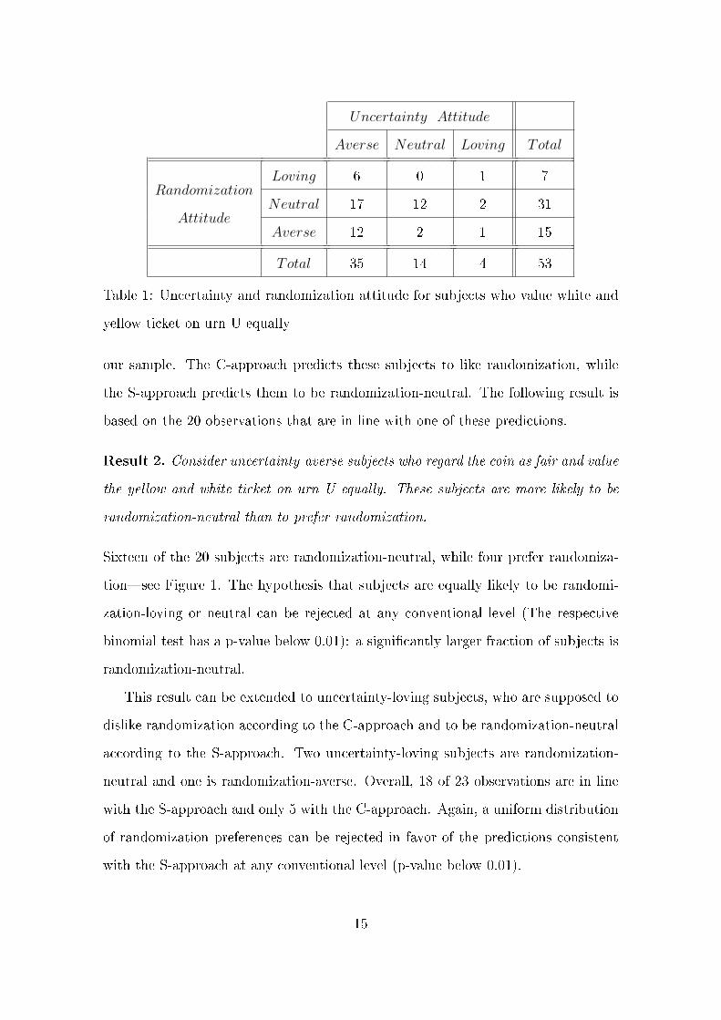
Table 1: Uncertainty and randomization attitude for subjects who value white and

yellow ticket on urn U equally

our sample. The C-approach predicts these subjects to like randomization, while

the S-approach predicts them to be randomization-neutral. The following result is

based on the 20 observations that are in line with one of these predictions.

Result 2. Consider uncertainty-averse subjects who regard the coin as fair and value

the yellow and white ticket on urn U equally. These subjects are more likely to be

randomization-neutral than to prefer randomization.

Sixteen of the 20 subjects are randomization-neutral, while four prefer randomiza-

tion�see Figure 1. The hypothesis that subjects are equally likely to be randomi-

zation-loving or neutral can be rejected at any conventional level (The respective

binomial test has a p-value below 0.01): a signi�cantly larger fraction of subjects is

randomization-neutral.

This result can be extended to uncertainty-loving subjects, who are supposed to

dislike randomization according to the C-approach and to be randomization-neutral

according to the S-approach. Two uncertainty-loving subjects are randomization-

neutral and one is randomization-averse. Overall, 18 of 23 observations are in line

with the S-approach and only 5 with the C-approach. Again, a uniform distribution

of randomization preferences can be rejected in favor of the predictions consistent

with the S-approach at any conventional level (p-value below 0.01).

15

05

10

15

Fre

quency

averse neutral lovingrandomization attitude amongst uncertainty averse

Figure 1: Randomization attitudes of uncertainty-averse subjects who regard the

coin as fair and value white and yellow ticket on urn U equally

5.2 Robustness

The theoretical results, which underpin Hypothesis 1 and 2, only apply to subjects

with speci�c preferences. Consequently, Result 2 and 3 are based on a selected

sample of subjects, which may not only di�er by their preferences but by other

characteristics.

We check whether any selection on observables has taken place by running two

probit regressions. Hypothesis 1 requires subjects to be indi�erent between the

yellow and white ticket on urn U. This indi�erence, however, does not seem to be

related to observables: the null hypothesis that no observable a�ects the probability

of being indi�erent cannot be rejected (p-value of the likelihood ratio test: 0.43,

see Table 4 in the appendix). For Hypothesis 2, subjects must additionally regard

the coin as fair. This time there is some indication that observables a�ect selection

(p-value for the likelihood ratio test: 0.04). More speci�cally, subjects who correctly

compute the probability of two independently thrown dice (variable: stats knowledge

2) are signi�cantly more likely to be in the sample (see Table 5 in the appendix).

16

Accordingly, we expect these subjects to be more in line with theoretical predictions.

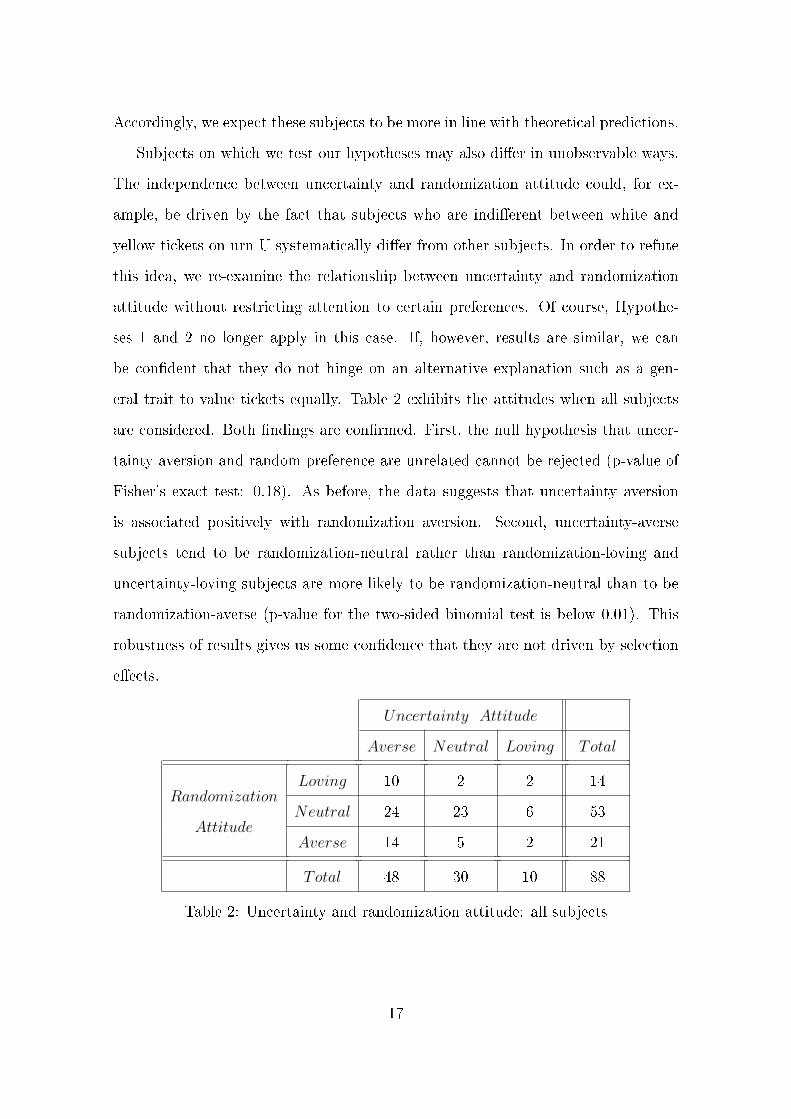
Subjects on which we test our hypotheses may also di�er in unobservable ways.

The independence between uncertainty and randomization attitude could, for ex-

ample, be driven by the fact that subjects who are indi�erent between white and

yellow tickets on urn U systematically di�er from other subjects. In order to refute

this idea, we re-examine the relationship between uncertainty and randomization

attitude without restricting attention to certain preferences. Of course, Hypothe-

ses 1 and 2 no longer apply in this case. If, however, results are similar, we can

be con�dent that they do not hinge on an alternative explanation such as a gen-

eral trait to value tickets equally. Table 2 exhibits the attitudes when all subjects

are considered. Both �ndings are con�rmed. First, the null hypothesis that uncer-

tainty aversion and random preference are unrelated cannot be rejected (p-value of

Fisher's exact test: 0.18). As before, the data suggests that uncertainty aversion

is associated positively with randomization aversion. Second, uncertainty-averse

subjects tend to be randomization-neutral rather than randomization-loving and

uncertainty-loving subjects are more likely to be randomization-neutral than to be

randomization-averse (p-value for the two-sided binomial test is below 0.01). This

robustness of results gives us some con�dence that they are not driven by selection

e�ects.

Uncertainty Attitude

Averse Neutral Loving Total

RandomizationLoving 10 2 2 14

AttitudeNeutral 24 23 6 53

Averse 14 5 2 21

Total 48 30 10 88

Table 2: Uncertainty and randomization attitude: all subjects

17

5.3 Other �ndings

In addition to these results, which directly relate to our hypotheses, we also want

to report on two additional and unexpected �ndings.

The �rst concerns randomization- and uncertainty-averse subjects. We expected

to �nd very few of them because they are not backed by the most prevalent models

of uncertainty-aversion�irrespective of whether they are axiomatized in the S- nor

in the C-approach.

Result 3. A non-negligible fraction of uncertainty-averse subjects dislikes random-

ization.

Of the 48 uncertainty-averse subjects, 14 express a dislike for randomization (see

Table 2). If we restrict attention to subjects for whom behavior can be predicted

using the S- or C-approach because they regard the coin as fair and have no color

preference on urn U, a similar picture emerges: 9 out of 29 uncertainty-averse sub-

jects prefer the pure tickets over the mixture�see Figure 1. In both cases, the share

is statistically not distinguishable at any conventional level from the naive predic-

tion by someone who does not know any of these theories and expects randomization

aversion to occur in a third of the cases.

The observed combination of randomization and uncertainty aversion is puzzling.

The respective subjects prefer to know whether the ticket, which they receive, is

white or yellow�although they are indi�erent between receiving a white and a

yellow ticket. Possible reasons are that knowing the color has a value in itself to

these subjects, that they assign lower values to tickets when complexity is involved,

or that they dislike the loss of control associated with the coin.7

7Keren and Teigen (2008) argue that such decision makers like to maintain control. Dittmann,

Kübler, Maug, and Mechtenberg (2008) �nd that experimental subjects are willing to pay a pre-

mium for exerting the right to vote even if the probability that this a�ects the outcome is very

low. On the other hand, Cettolin and Riedl (2008) observe that subjects prefer a random draw

when having to decide between risky and uncertain prospects.

18

Our second �nding is related to a theoretical result by Klibano� (2001). Klibano�

shows that if a randomizing device is stochastically independent and Choquet-

expected utility preferences are modeled in the S-approach, preferences cannot ex-

hibit uncertainty-aversion. This implies for our context that subjects whose prefer-

ences can be modeled using the S-approach because they are uncertainty-averse and

randomization-neutral should regard the coin to be correlated with urn U. In order

to test this, we constructed a bet in which a ball is drawn from urn U; the subject

then receives a head ticket if the ball is yellow and its certainty equivalent of a head

ticket if the ball is white. Subjects who view coin and ball draw as independent

should attach the same value to this bet, which we call combination ticket, and

a head ticket. We restrict attention to subjects who regard the coin as fair, value

white and yellow tickets on urn U equally, and are randomization-neutral. Following

Klibano�'s argument, we expect these subjects to be less likely to attach di�erent

values to the combination and head ticket if they are uncertainty-neutral. Indeed,

the respective share of subjects is lower amongst uncertainty-neutral subjects (20%)

than amongst other uncertainty-averse subjects (31%); however, the di�erence is

not signi�cant at any conventional level (p-value of one-sided two-sample test of

proportion: 0.26). More surprising, the proportion of all subjects who value the

head ticket more than the combination ticket is 37%. Put di�erently, these subjects

prefer a head ticket to a mixture of head ticket and its certainty equivalent. While

a possible explanation is that subjects regard coin throw and ball draw as corre-

lated, there is an interesting link between this �nding and randomization aversion:

subjects who favor the heads to the combination ticket also tend to favor tickets

of a speci�c color to the chameleon ticket (Kendall's τb=0.1966, p-value: 0.0559).

A �rst tentative conclusion may thus be that both results are driven by the same

explanation, e.g., a distaste for complexity.

19

6 Conclusions

We started our analysis with the classical observation from the two-color experi-

ment by Ellsberg (1961): individuals prefer to bet in situations about which they

are better informed. Existing explanations for such behavior often rely on the idea

that access to an objective randomization device mitigates the problem of lack-

ing information. Accordingly, uncertainty-averse individuals are supposed to prefer

randomization. The data from our experiment, however, does not support this

view: there is no negative association between uncertainty and randomization atti-

tude. Uncertainty-averse subjects are more likely to be randomization-neutral than

randomization-loving. Their behavior is consistent with modeling uncertainty aver-

sion in a Savage framework (S-approach) rather than using the consequence space in

the tradition of Anscombe-Aumann (C-approach). None of the prevailing theories

of uncertainty aversion, however, explains another phenomenon observed in our ex-

periment: a considerable number of uncertainty-averse subjects exhibits a contempt

for randomization. This could indicate that for many subjects, the randomization

device does not reduce but enhances the problem of missing information.

20

Appendix

Uncertainty attitude

In this section we introduce a notation and show that under mild conditions our

de�nition of uncertainty attitudes coincides with the de�nition proposed by Epstein

(1999).

Notation

All circumstances that a�ect subjects payo�s are represented by a state space S. An

event, E, is a subset of S. The set of all possible payo�s is denoted by X. Objects

of choice are bets, denoted by f , which are mappings from the state space S, to the

set of all possible payo�s X. Binary bets xEy assign a constant payment f(s) = x

to each state of nature s in E and a constant payment g(s) = y to each state of

nature s in S \E, with x, y ∈ X. More general, bets fEg assign a payo� f(s) to each

state of nature s in E and a payo� g(s) to each state of nature s in S \ E. Let F

be a set of all possible bets and let < be a binary relation that represents subjects'

preferences over F . For any bet f, g, h ∈ F we write f < {g, h} to denote f < g

and f < h.

Result

Recently, Epstein (1999) proposed a two-stage approach to de�ne uncertainty at-

titudes.8 In this approach �rst a comparative notion of uncertainty aversion and

then an absolute de�nition for uncertainty aversion is established. The comparative

de�nition is based on the following idea: if a subject prefers an unambiguous bet

to an ambiguous one, then a more uncertainty-averse subject will do the same. For

Epstein, a bet is unambiguous if its payo�s depend on exogenously given unambigu-

8The two-stage approach is used also by Ghirardato and Marinacci (2002).

21

ous events, i.e., events which randomness is objectively known (for instance a fair

coin, a roulette wheel, etc.). Let Fua be the set of unambiguous bets. Consider two

preference relations <1 and <2. Then, <1 is said to be more uncertainty-averse than

<2 if for any unambiguous bet h ∈ Fua and any bet e ∈ F :

h <1 (�1)e ⇒ h <2 (�2)e. (1)

An absolute de�nition of uncertainty attitudes is derived by choosing a benchmark

order for uncertainty-neutral preferences. Epstein (1999) uses for the benchmark or-

der, <PS, preferences that are probabilistically sophisticated in the sense of Machina

and Schmeidler (1992). According to this theory subjects' subjective beliefs are rep-

resented by an unique and additive probability distribution, but preferences do not

need to have expected utility representation. Then, < is said to be uncertainty-

averse if there exists a probabilistically sophisticated preference relation <PS such

that for any h ∈ Fua and any bet e ∈ F :

h <PS (�PS)e ⇒ h < (�)e. (2)

Conversely, < is said to be uncertainty-loving if there exists a probabilistically so-

phisticated preference relation <PS such that for any h ∈ Fua and any bet e ∈ F :

h 4PS (≺PS)e ⇒ h 4 (≺)e. (3)

If < is both uncertainty-averse and uncertainty-loving then it is uncertainty-neutral.9

Proposition 1. If urn K is viewed as unambiguous, then our empirical de�nition

coincides with that of Epstein (1999).

Proof. Throughout, we consider a subject with the following preferences:

qK < rK and sU < tU , (4)

9Ghirardato and Marinacci (2002) use for the benchmark order preferences respecting subjec-

tive expected utility representation à la Savage (1954). As unambiguous bets they consider only

constant bets, i.e., h(s) = x for any s ∈ S with x ∈ X.

22

where qK , rK ∈ {yK , wK} and sU , tU ∈ {yU , wU}. Let QK , RK ∈ {Y K ,WK}, and

SU , TU ∈ {Y U ,WU} be the corresponding events. Suppose that subjects being

informed about the exact composition of white and yellow balls in the urn K view

it as unambiguous. In this situation payo�s of the yellow ticket yK and the white

ticket wK depend upon the realization of unambiguous events Y K andWK to which

subjects assign probabilities π[Y K ] and π[WK ]. Thus, both tickets are unambiguous

bets, i.e. yK , wK ∈ Fua.

Let us �rst consider the behavior of an uncertainty-neutral subject according to

Epstein. Note that any probabilistically sophisticated order is equivalent to an order

based on probabilities. All orders based on probabilities fall into one of the three

following cases:

qK ∼PS sU <PS tU ∼PS rK , (5)

qK �PS sU <PS tU �PS rK , (6)

sU �PS qK <PS rK �PS tU . (7)

The subsequent proof proceeds in three steps. In Step 1, we show that uncertainty-

averse subjects according to De�nition 2 are also uncertainty-averse according to

Epstein. In Step 2 and 3, we do the same for uncertainty-loving and uncertainty-

neutral subjects.

Step 1: Uncertainty aversion.

By assumption, qK < sU and rK < tU with at least one strict preference relation

(�). We examine two cases: qK ∼ rK and qK � rK .

Case 1: qK ∼ rK . In this case, we obtain:

qK ∼ rK < sU < tU , (8)

with at least one strict preference. Take <PS with π(QK) = πPS(QK) as in (5) such

that:

qK ∼PS sU ∼PS tU ∼PS rK . (9)

23

Comparing < from (8) with <PS as in (9), we get:

qK ∼PS {rK , sU , tU} ⇒ qK ∼ {rK} < {sU} < {tU},

rK ∼PS {qK , sU , tU} ⇒ rK ∼ {qK} < {sU} < {tU},

where at least one of the weak preference is strict in each row. Thus, there exists

<PS such that < is more uncertainty-averse then <PS according to Epstein�see (2).

Case 2: qK � rK . In this case, one of the following can occur:

qK � rK < sU < tU , or (10)

qK < sU � rK < tU , (11)

with at least one strict preference in each case. Take <PS with π(QK) = πPS(QK)

as in (5) such that:

qK ∼PS sU �PS tU ∼PS rK .

Comparing this <PS with < as in (10), we get:

qK ∼PS {sU} �PS {rK , tU} ⇒ qK � {rK , sU , tU},

rK ∼PS {tU} ⇒ rK < {sU , tU}.

Analogously, the comparison with < as in (11), yields:

qK ∼PS {sU} �PS {rK , tU} ⇒ qK < {sU} < {rK , tU},

rK ∼PS {tU} ⇒ rK � {tU}.

Thus, for preference ordering < as in (10) and as in (11), there exists <PS such that

< is more uncertainty-averse then <PS according to Epstein�see (2). Summarizing

both cases, we have seen that for qK < sU or rK < tU with at least one strict

preference relation (�), < is uncertainty-averse according to Epstein.

Step 2: Uncertainty loving.

By assumption, qK 4 sU and rK 4 tU with at least one strict preference relation

(≺). Again, we consider two cases: qK ∼ rK and qK � rK .

24

Case 1: qK ∼ rK . In this case, we obtain:

sU < tU < qK ∼ rK , (12)

with at least one strict preference. Take <PS with π(QK) = πPS(QK) as in (5) such

that:

qK ∼PS sU ∼PS tU ∼PS rK . (13)

Comparing the respective <PS with < from (12), we obtain:

qK ∼PS {rK , sU , tU} ⇒ qK ∼ {rK} 4 {sU} 4 {tU},

rK ∼PS {qK , sU , tU} ⇒ rK ∼ {qK} 4 {sU} 4 {tU},

where at least one of the weak preference is strict in each row. Thus, there exists

<PS such that < is less uncertainty-averse then <PS. Hence, < is uncertainty-loving

according to Epstein�see (3).

Case 2: qK � rK . In this case, one of the following can occur:

sU < tU < qK � rK , or (14)

sU < qK � tU < rK , (15)

with at least one strict preference in each case. Take <PS with π(QK) = πPS(QK)

as in (5) such that:

qK ∼PS sU �PS tU ∼PS rK . (16)

Comparing this <PS with < from (14), we obtain:

qK ∼PS {sU} ⇒ qK 4 {tU} 4 {sU},

rK ∼PS {tU} ≺ {sU , qK} ⇒ rK ≺ {qK , tU , sU}.

Comparing the same benchmark with < from (15), we get:

qK ∼PS {sU} ⇒ qK 4 {sU},

rK ∼PS {tU} ≺ {sU , qK} ⇒ rK 4 {tU} ≺ {qK , sU}.

Thus, in both cases, there exists <PS such that < is less uncertainty-averse then

<PS and we conclude that < is uncertainty-loving according to Epstein�see (3).

25

Hence, if qK 4 sU or rK 4 tU with at least one strict preference relation (≺), then

< is uncertainty-loving according to Epstein.

Step 3: Uncertainty neutrality.

Suppose now that qK ∼ sU and rK ∼ tU , or qK � sU and rK ≺ tU , or qK ≺ sU and

rK � tU . Then one of the following can occur:

qK ∼ sU < tU ∼ rK , (17)

qK � sU < tU � rK , (18)

sU � qK < rK � tU . (19)

Take <PS with π(QK) = πPS(QK) as in (5), in (6) and in (7). Any < as in (17), in

(18) and in (19) is order equivalent with <PS as in (5), in (6) and in (7), respectively.

Thus, for any < as in (17), in (18) and in (19) there exists <PS such that both is

true: < is more uncertainty-averse than <PS and < is less uncertainty-averse than

<PS. Therefore, < is uncertainty-neutral according to Epstein.

26

Table 3: Variable de�nitions

Variable name Dummy variables which take the value one if...

no color preference subject indi�erent between white and yellow ticket for urn U

coin fair subject regards coin as fair

male subject male

economics student subject studies economics

business student subject studies business administration

stats knowledge 1 Prob(10-sided fair dice shows 2 or less) computed correctly

stats knowledge 2 Prob(two 10-sided fair dice show two ones) computed correctly

stats knowledge 3 Prob(10-sided fair dice shows 4| even number)* computed correctly

stats knowledge 4 Prob(10-sided fair dice shows 4| odd number) computed correctly

stats knowledge 5 average payo� of two bets, one which pays 100 in case of even

the other pays 100 in case of odd computed correctly

cognitive ability 1 correct answer to... A bat and a ball cost $1.10. The bat

costs $1.00 more than the ball. How much does the ball cost?

cognitive ability 2 correct answer to... 5 machines need 5 min to produce 5 pieces.

How long do 100 machines need to produce 100 pieces?

cognitive ability 3 correct answer to... A lake is covered by sea roses. The covered

surface doubles every day. If 48 days are needed until the lake is

entirely covered, how long does it take until half the lake is covered?

Variable name Subjective agreement with following statements

on a scale from 1 (totally disagree) to 7 (totally agree)

superstition There are unlucky numbers.

god God is important in my life.

religion Religion gives me strength and support.

fate What one achieves in life depends on fate and luck.

* Prob(A|B) denotes the conditional probability of event A to occur after the occurence of B.

27

Table 4: Selection on observables: Hypothesis 1

Dependent variable: No color preference on urn U (yU ∼ wU)

Variable Coefficient Stand. Error p− value

male 0.150 0.116 0.196

economics student -0.214 0.194 0.271

business student 0.188 0.130 0.147

stats knowledge 1 -0.021 0.181 0.906

stats knowledge 2 0.143 0.131 0.275


stats knowledge 4 -0.124 0.177 0.480

stats knowledge 5 -0.046 0.143 0.747

cognitive ability1 -0.108 0.131 0.409


cognitive ability3 0.022 0.150 0.883

superstitious -0.017 0.042 0.681

god 0.083 0.069 0.222

religion -0.104 0.072 0.144

fate -0.004 0.038 0.923

Number of Obs. = 88

Log likelihood = -51.495

Prob > χ2 = 0.43

Pseudo R2 = 0.129

Signi�cance levels:*(5%), **(2%), ***(1%)

28

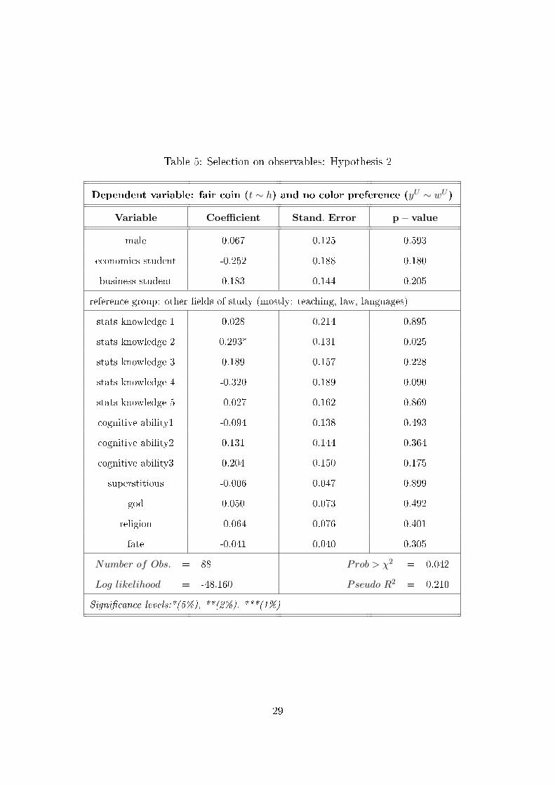
Table 5: Selection on observables: Hypothesis 2

Dependent variable: fair coin (t ∼ h) and no color preference (yU ∼ wU)

Variable Coefficient Stand. Error p− value

male 0.067 0.125 0.593

economics student -0.252 0.188 0.180

business student 0.183 0.144 0.205

reference group: other �elds of study (mostly: teaching, law, languages)


stats knowledge 2 0.293* 0.131 0.025


stats knowledge 4 -0.320 0.189 0.090

stats knowledge 5 -0.027 0.162 0.869




superstitious -0.006 0.047 0.899

god 0.050 0.073 0.492

religion -0.064 0.076 0.401

fate -0.041 0.040 0.305

Number of Obs. = 88

Log likelihood = -48.160

Prob > χ2 = 0.042

Pseudo R2 = 0.210

Signi�cance levels:*(5%), **(2%), ***(1%)

29

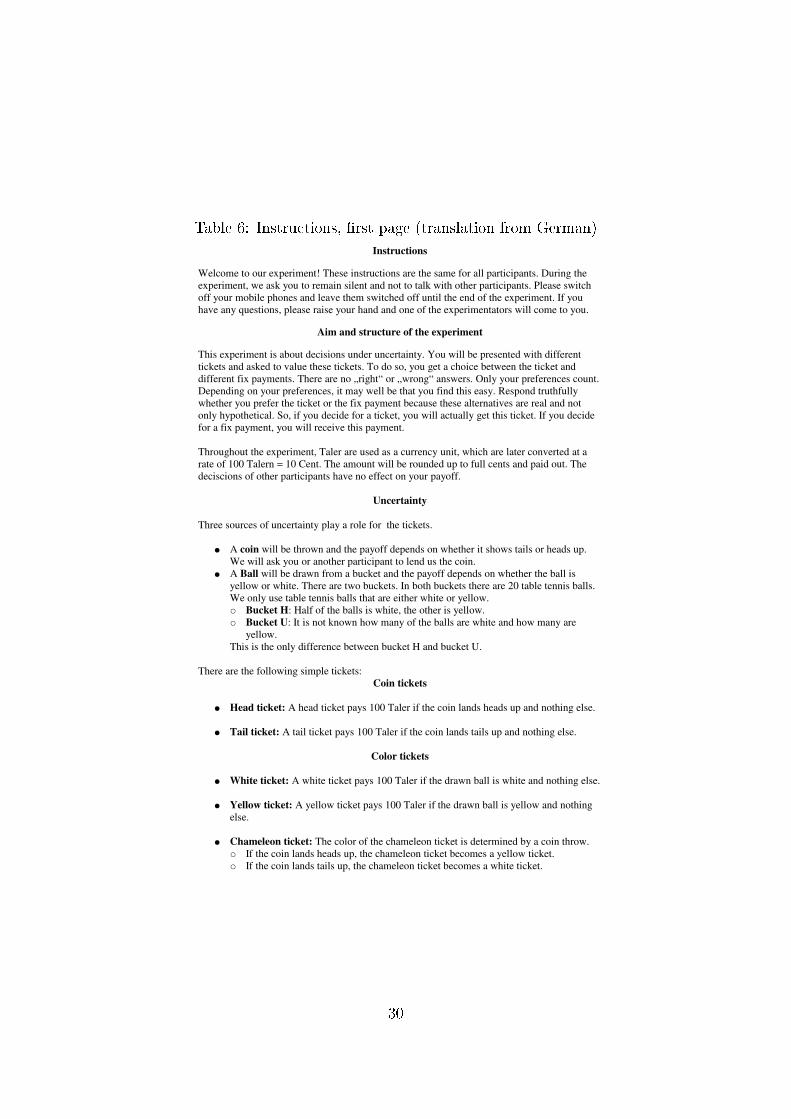
Table 6: Instructions, �rst page (translation from German)

Instructions

Welcome to our experiment! These instructions are the same for all participants. During the

experiment, we ask you to remain silent and not to talk with other participants. Please switch

off your mobile phones and leave them switched off until the end of the experiment. If you

have any questions, please raise your hand and one of the experimentators will come to you.

Aim and structure of the experiment

This experiment is about decisions under uncertainty. You will be presented with different

tickets and asked to value these tickets. To do so, you get a choice between the ticket and

different fix payments. There are no „right“ or „wrong“ answers. Only your preferences count.

Depending on your preferences, it may well be that you find this easy. Respond truthfully

whether you prefer the ticket or the fix payment because these alternatives are real and not

only hypothetical. So, if you decide for a ticket, you will actually get this ticket. If you decide

for a fix payment, you will receive this payment.

Throughout the experiment, Taler are used as a currency unit, which are later converted at a

rate of 100 Talern = 10 Cent. The amount will be rounded up to full cents and paid out. The

deciscions of other participants have no effect on your payoff.

Uncertainty

Three sources of uncertainty play a role for the tickets.

● A coin will be thrown and the payoff depends on whether it shows tails or heads up.

We will ask you or another participant to lend us the coin.

● A Ball will be drawn from a bucket and the payoff depends on whether the ball is

yellow or white. There are two buckets. In both buckets there are 20 table tennis balls.

We only use table tennis balls that are either white or yellow.

○ Bucket H: Half of the balls is white, the other is yellow.

○ Bucket U: It is not known how many of the balls are white and how many are

yellow.

This is the only difference between bucket H and bucket U.

There are the following simple tickets:

Coin tickets

● Head ticket: A head ticket pays 100 Taler if the coin lands heads up and nothing else.

● Tail ticket: A tail ticket pays 100 Taler if the coin lands tails up and nothing else.

Color tickets

● White ticket: A white ticket pays 100 Taler if the drawn ball is white and nothing else.

● Yellow ticket: A yellow ticket pays 100 Taler if the drawn ball is yellow and nothing

else.

● Chameleon ticket: The color of the chameleon ticket is determined by a coin throw.

○ If the coin lands heads up, the chameleon ticket becomes a yellow ticket.

○ If the coin lands tails up, the chameleon ticket becomes a white ticket.

30

Table 7: Instructions, second page (translation from German)

For color tickets, it will be specified to which bucket they apply: H or U. A yellow ticket for

bucket U thus means that a ball is drawn from the bucket with unknown proportions and that

100 Taler are paid if this ball is yellow..

Apart from these tickets there will be other variations that you will get to know during the

experiment.

Decitions and the value of tickets

For each ticket there will be a set of questions. For example:

Head ticket Fix payment of ...

Question 1 ( ) ...68 Taler ( )

Question 2 ( ) ...96 Taler ( )

For Question 1 you have to decide between a head ticket or a fix payment of 68 Taler. For

Question 2 between a head ticket and 96 Taler.

For each question concerning the same color ticket, a new ball will be drawn; already drawn

balls are replaced. For each question concerning a coin ticket, the coin is thrown. All draws are

hence completely independent of each other. Your payoff is hence maximized if you answer

according to the value of the ticket.

If for example the ticket is worth 80 Taler to you, then you should prefer the ticket to a fix

payment of 68 Taler (otherwise you lose 12 Taler). If you have the choice between the ticket

and 96 Talern, you should choose 96 Taler (otherwise you lose sixteen Taler).

Input assistant

The close relationship between the value of a ticket and your decisions is used by the program

to facilitate the input. You have the possibility to directly specify the value of a ticket in steps

of 5 Taler using a slider. The program then automatically marks the corresponding decisions.

If you want to you can change these decisions. The program then adjusts the value of the

ticket. Note that the value of the ticket cannot always be computed. For example, if you select

a fix payment of 58 Taler rather than the ticket but also choose the ticket rather than a fix

payment of 63 Taler, this means that the ticket is worth less than 58 Taler to you but also more

than 63 Taler. In this case, it is impossible to determine the value of the ticket to you.

Sequence

The experiment starts with a few problems, which should help you to acquaint yourself with

the different types of questions. Moreover, we want to ensure that you have not misunderstood

the instructions. Decisions during this part do not affect your payoffs. After the understanding

part, the main part of the experiment begins. The decision during this part are for real. They

hence affect your payoffs. Finally, we ask you some general questions. Altogether the

experiment will take 90 minutes. You have enough time for your answers since the draws only

start if all participants are ready.

31

Figure 2: Valuation screen for head ticket (in German)

32

References

Anscombe, F. J., and R. J. Aumann (1963): �A De�nition of Subjective Proba-

bility,� Annals of Mathematical Statistics, 34(1), 199�105.

Becker, G. M., M. H. DeGroot, and J. Marschak (1964): �Measuring Utility

by a Single-Response Sequential Method,� Behavioral Science, 9(3), 226�232.

Camerer, C., and M. Weber (1992): �Recent Developments in Modelling Pref-

erences: Uncertainty and Umbiguity,� Journal of Risk and Uncertainty, 5(4),

325�370.

Cettolin, E., and A. Riedl (2008): �Changing Ambiguity Attitudes and a Pref-

erence for Indi�erence,� unpublished manuscript, Maastricht University.

Dittmann, I., D. Kübler, E. Maug, and L. Mechtenberg (2008): �Why

Votes Have a Value,� Discussion Paper 68, Department of Economics, Humboldt

University Berlin.

Dow, J., and S. R. D. C. Werlang (1994): �Nash Equilibrium under Knightian

Uncertainty: Breaking Down Backward Induction,� Journal of Economic Theory,

64(2), 305�324.

Eichberger, J., and D. Kelsey (1996): �Uncertainty Aversion and Preference

for Randomisation,� Journal of Economic Theory, 71(1), 31�43.

Eichberger, J., and D. Kelsey (2000): �Non-Additive Beliefs and Strategic

Equilibria,� Games and Economic Behavior, 30(2), 183 � 215.

Ellsberg, D. (1961): �Risk, Ambiguity, and the Savage Axioms,� The Quarterly

Journal of Economics, 75(4), 643�669.

Epstein, L. G. (1999): �A De�nition of Uncertainty Aversion,� Review of Economic

Studies, 66(3), 579�608.

33

(2009): �Three Paradoxes for the `Smooth Ambiguity' Model of Preference,�

Working paper, Department of Economics, University of Boston.

Fischbacher, U. (2007): �Zurich Toolbox for Research in Economic Experiments,�

Experimental Economics, 10(2), 171�178.

Ghirardato, P. (1997): �On Independence for Non-Additive Measures with Fubini

Theorem,� Journal of Economic Theory, 73(2), 261�291.

Ghirardato, P., and M. Marinacci (2002): �Ambiguity Made Precise: A Com-

perative Foundation,� Journal of Economic Theory, 102(2), 251�289.

Gilboa, I. (1987): �Expected Utility With Purely Subjective Non-Additive Proba-

bilities,� Journal of Mathematical Economics, 16(1), 65�88.

Gilboa, I., and D. Schmeidler (1989): �Maximin Expected Utility with Non-

Unique Prior,� Journal of Mathematical Economics, 18(2), 141�153.

Halevy, Y. (2007): �Ellsberg Revisited: An Experimental Study,� Econometrica,

75(2), 503�536.

Hey, J. D., G. Lotito, and A. Maffioletti (2008): �The Descriptive and Pre-

dictive Adequacy of Theories of Decision Making Under Uncertainty/Ambiguity,�

Discussion Papers 08/04, Department of Economics, University of York.

Holt, C. A. (1986): �Preference Reversals and the Independence Axiom,� American

Economic Review, 76(3), 508�15.

Holt, C. A., and S. K. Laury (2002): �Risk Aversion and Incentive E�ects,�

American Economic Review, 92(5), 1644�1655.

Karni, E., and Z. Safra (1987): �'Preference Reversal' and the Observability of

Preferences by Experimental Methods,� Econometrica, 55(3), 675�85.

34

Keren, G., and K. H. Teigen (2008): �Decisions by Coin Toss and the Limits of

Rationality,� unpublished manuscript, Tilburg Institute for Behavioral Economics

Research.

Klibanoff, P. (1996): �Uncertainty, Decisions and Normal Form Games,� unpub-

lished manuscript, Kellog Graduate School of Economics, Northwestern Univer-

sity, Chicago.

(2001): �Stochastically Independent Randomization and Uncertainty Aver-

sion,� Economic Theory, 18(3), 605�620.

Klibanoff, P., M. Marinacci, and S. Mukerji (2005): �A Smooth Model of

Decision Making under Ambiguity,� Econometrica, 73(6), 1849�1892.

(2009): �On the Smooth Ambiguity Model: A Reply,� Working paper,

Department of Economics, University of Oxford.

Lo, K. C. (1996): �Equlibrium in Beliefs under Uncertainty,� Journal of Economic

Theory, 71(2), 443�484.

Maccheroni, F., M. Marinacci, and A. Rustichini (2006): �Ambiguity Aver-

sion, Robustness, annd the Variational Representation of Preferences,� Economet-

rica, 74(6), 1447�1498.

Machina, M. J., and D. Schmeidler (1992): �A More Robust De�nition of

Subjective Probability,� Econometrica, 60(4), 745�80.

Marinacci, M. (2000): �Ambiguous Games,� Games and Economic Behavior,

31(2), 191 � 219.

Raiffa, H. (1961): �Risk, Ambiguity, and the Savage Axioms: Comment,� The

Quarterly Journal of Economics, 75(4), 690�694.

Sarin, R. K., and P. Wakker (1992): �A Simple Axiomatization of Nonadditive

Expected Utility,� Econometrica, 60(6), 1255�1272.

35

Savage, L. J. (1954): The Foundation of Statistics. Wiley, New York.

Schmeidler, D. (1989): �Subjective Probability and Expected Utility Without

Additivity,� Econometrica, 57(3), 571�587.

Segal, U. (1988): �Does the Preference Reversal Phenomenon Necessarily Contra-

dict the Independence Axiom?,� American Economic Review, 78(1), 233�36.

Trautmann, S. T., F. M. Vieider, and P. P. Wakker (2009): �Preference

Reversals for Ambiguity Aversion,� Tilburg Institute for Behavioral Economics

Research, Tilburg University.

36

Documents

Attitudes towards Uncertainty and Randomization: An ... · (1987) and Sarin and Wakker (1992). 2 See Ghirardato (1997) and Klibano (2001) for theoretical contributions on the role