HAL Id: hal-00196504https://hal.archives-ouvertes.fr/hal-00196504

Submitted on 12 Dec 2007

HAL is a multi-disciplinary open accessarchive for the deposit and dissemination of sci-entific research documents, whether they are pub-lished or not. The documents may come fromteaching and research institutions in France orabroad, or from public or private research centers.

L’archive ouverte pluridisciplinaire HAL, estdestinée au dépôt et à la diffusion de documentsscientifiques de niveau recherche, publiés ou non,émanant des établissements d’enseignement et derecherche français ou étrangers, des laboratoirespublics ou privés.

Atomic force microscopy imaging and related issues insignal processing: a preliminary work

Charles Soussen, David Brie, Fabien Gaboriaud, Cyril Kessler

To cite this version:Charles Soussen, David Brie, Fabien Gaboriaud, Cyril Kessler. Atomic force microscopy imaging andrelated issues in signal processing: a preliminary work. 22nd IAR annual meeting, Nov 2007, Grenoble,France. pp.CDROM, 2007. <hal-00196504>

ATOMIC FORCE MICROSCOPY IMAGING

AND RELATED ISSUES IN SIGNAL

PROCESSING: A PRELIMINARY WORK

Charles Soussen ∗ David Brie ∗ Fabien Gaboriaud ∗∗

Cyril Kessler ∗

∗ Centre de Recherche en Automatique de Nancy (CRAN,UMR 7039, Nancy-University, CNRS), Boulevard desAiguillettes, B.P. 239, F-54506 Vandœuvre-les-Nancy,

France∗∗ Laboratoire de Chimie Physique et Microbiologie pour

l’Environnement (LCPME, UMR 7564, Nancy-University,CNRS), 405, rue de Vandœuvre, 54600 Villers-les-Nancy,

France

Abstract: Interatomic and intermolecular forces have been extensively studied,for their ability to understand the processes at the interface between solidsand aqueous solutions. In particular, atomic force microscopy (AFM) generatestridimensional images and force profiles at nanometric scale, whatever the natureof the samples (biological, organic, mineral). An AFM microscope affords themeasurement of interatomic forces exerting between a probe associated to acantilever and a chemical sample. A force spectrum f(z) shows the evolution ofthese forces as a function of the distance z between the probe and the sample.This is a pointwise analysis of the sample, obtained by measuring the cantileverdeflection with respect to the probe-sample distance. A reproduction of thispointwise analysis, in conjunction with the scan of the sample surface yields aforce-volume image f(x, y, z). This image is composed of the collection of forcespectra f(z) on a grid (x, y) representing the sample surface. Today, the analysisand interpretation of a force-volume image remains mainly descriptive. In thispaper, we introduce a signal processing formulation, which aims at a preciseand automatic characterization of each pixel (xi, yi) of the sample surface. Theseproblems include the decomposition of a force spectrum into elementary patterns,and the factorization of a force-volume image. We discuss the ability of standardsignal processing methods to solve these problems, and we illustrate the discussionby means of experimental data.

Keywords: Nanotechnology, atomic force microscopy (AFM), force-volumeimaging, tridimensional signals, convolutive mixture of signals, optimization ofmultidimensional criteria.

1. INTRODUCTION

Interatomic and intermolecular forces have beenextensively studied, for their ability to under-stand the processes at the interface betweensolids and aqueous solutions. During the lastdecades, the development of near field micro-scopies has afforded to determine in situ localphysico-chemical properties (electric, magnetic,vibration, forces) (Wiesendanger, 1994). In partic-ular, atomic force microscopy (AFM) is capable togenerate force profiles at nanometric scale, what-ever the nature of the samples (biological, organic,mineral), and tridimensional (3D) images, calledforce-volume images.

Atomic force microscopy was invented in 1986(Binnig, 1986) and the first prototype was ex-hibited a few months later (Binnig et al., 1986).This discovery has motivated a great numberof developments, at experimental and theoreti-cal levels (Giessibl, 2003). Simultaneously, forcespectroscopy appeared, with the ability to recordforce-volume images (Sokolov et al., 1999; Heinzand Hoh, 1999; Butt et al., 2005).

An AFM microscope is based on the measurementof interatomic forces exerting between a probeassociated to a cantilever and a sample. A forcespectrum f(z) shows the evolution of these forcesas a function of the distance z between the probeand the sample, as recorded from the piezo dis-placement. This is a pointwise analysis of thesample, obtained by measuring the cantilever de-flection with respect to (w.r.t.) the probe-sampledistance. A reproduction of this pointwise anal-ysis, in conjunction with the scan of the sam-ple surface yields a force-volume image f(x, y, z).This image is composed of the collection of forcespectra f(z) on a grid (x, y) which represents thesample surface.

Today, the analysis and interpretation of a force-volume image remains mainly descriptive; to ourknowledge, there is no signal processing methoddedicated to force-volume imaging. Such toolswould consist in:

(1) the 3D reconstruction of maps representingthe topology of nano-objects, or the physico-chemical properties. The topologic recon-struction is a difficult problem which has notreceived, to our sense, a satisfactory solution.Its resolution will lead to major advances inthe interpretation and exploitation of datagenerated by other techniques of near fieldmicroscopy (namely, optical techniques).

(2) the research of elementary physico-chemicalcomponents inside a force-volume image.When the sample to be analyzed is a mixtureof heterogeneous components, the problem isto determine their number, to identify them,

and to estimate their relative distribution inthe mixture by source separation techniques.The development of multilinear factorizationmethods offers new perspectives, since theyaim at decomposing multidimensional im-ages by means of lower dimension descrip-tors (Harshman et al., 2003). We can expectto retrieve elementary force interactions fromforce-volume images, and to provide theirspatial distribution and their evolution as afunction of physico-chemical conditions suchas pH or ionic strength.

In the following section, we will describe the ac-quisition of spectroscopic data using the AFMinstrument. We will emphasize the physical in-teractions occurring between the probe and thesample during a force profile acquisition, and giveparametric models (Heinz and Hoh, 1999). In Sec-tions 3, 4 and 5, we will introduce the analysis offorce spectra and force-volume images in terms ofsignal processing problems, e.g., the decomposi-tion of a signal into elementary patterns and thefactorization of a multidimensional image. We willillustrate these problems with a set of real data,corresponding to mineral colloidal particles whosechemical surface properties are heterogeneous andfar to be understood.

2. AFM MICROSCOPY

The operating modes of an AFM microscope arebased on the detection of interatomic forces (cap-illary, electrostatic, Van der Waals, friction) ex-erting between a cantilever-mounted probe anda sample surface. We generally distinguish twomodes of data acquisition.

2.1 Contact and intermittent imaging modes

The probe performs the scanning of the wholesample surface, hence providing two-dimensionaldata. Two distinct modes are available:

• the contact (or static) mode. The probe andthe sample remain in close contact duringthe raster scan. The contact mode directlyprovides the topology;

• the non contact mode. Typically, a variationof the interaction forces induces a variationof the resonant frequency of the cantilever,leading to a reduction of the oscillation am-plitude. A closed-loop control system main-tains the oscillation amplitude, as the feed-back control signal is used to move the probeup and down, and keeps constant the forceacting on the oscillation of the cantilever.Therefore, this mode yields isoforce images.

x

y

probe z0

z

(xi, yi)sample

x

y(xi, yi)sample

0

z

probe

(a) (b)

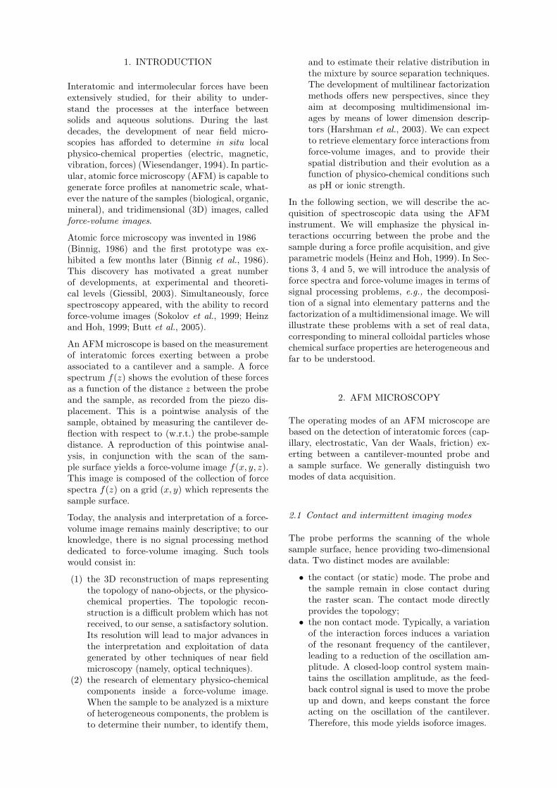
Fig. 1. Force spectroscopy. (a) At a pointwise location (xi, yi), the force measurements are collectedwhile the probe approaches, and then retracts from the sample. (b) For convenience, we pre-processthe data by reversing the orientation of the z axis, and we set z = 0 for the highest probe position.

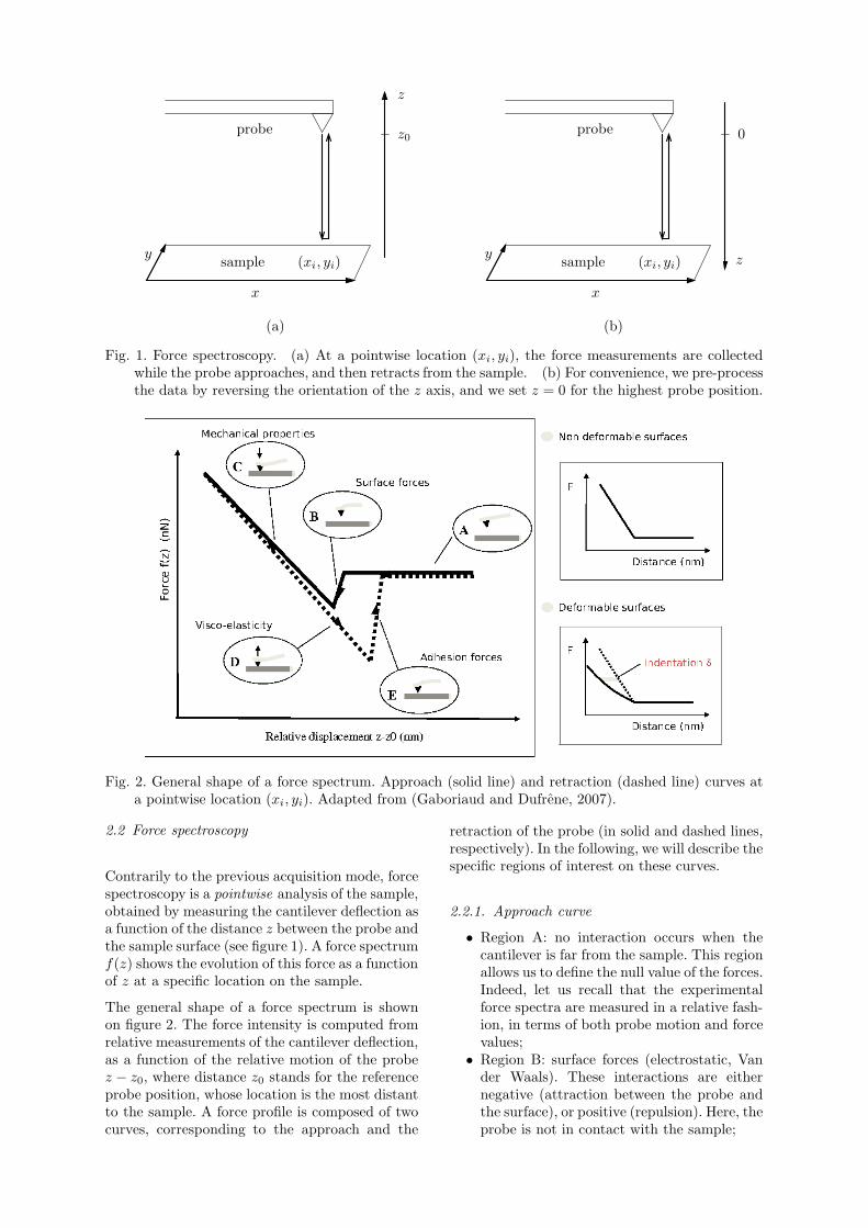
Fig. 2. General shape of a force spectrum. Approach (solid line) and retraction (dashed line) curves ata pointwise location (xi, yi). Adapted from (Gaboriaud and Dufrene, 2007).

2.2 Force spectroscopy

Contrarily to the previous acquisition mode, forcespectroscopy is a pointwise analysis of the sample,obtained by measuring the cantilever deflection asa function of the distance z between the probe andthe sample surface (see figure 1). A force spectrumf(z) shows the evolution of this force as a functionof z at a specific location on the sample.

The general shape of a force spectrum is shownon figure 2. The force intensity is computed fromrelative measurements of the cantilever deflection,as a function of the relative motion of the probez − z0, where distance z0 stands for the referenceprobe position, whose location is the most distantto the sample. A force profile is composed of twocurves, corresponding to the approach and the

retraction of the probe (in solid and dashed lines,respectively). In the following, we will describe thespecific regions of interest on these curves.

2.2.1. Approach curve

• Region A: no interaction occurs when thecantilever is far from the sample. This regionallows us to define the null value of the forces.Indeed, let us recall that the experimentalforce spectra are measured in a relative fash-ion, in terms of both probe motion and forcevalues;

• Region B: surface forces (electrostatic, Vander Waals). These interactions are eithernegative (attraction between the probe andthe surface), or positive (repulsion). Here, theprobe is not in contact with the sample;

Relative displacement z (nm)

Force f(z) (nN)

(a) (b)

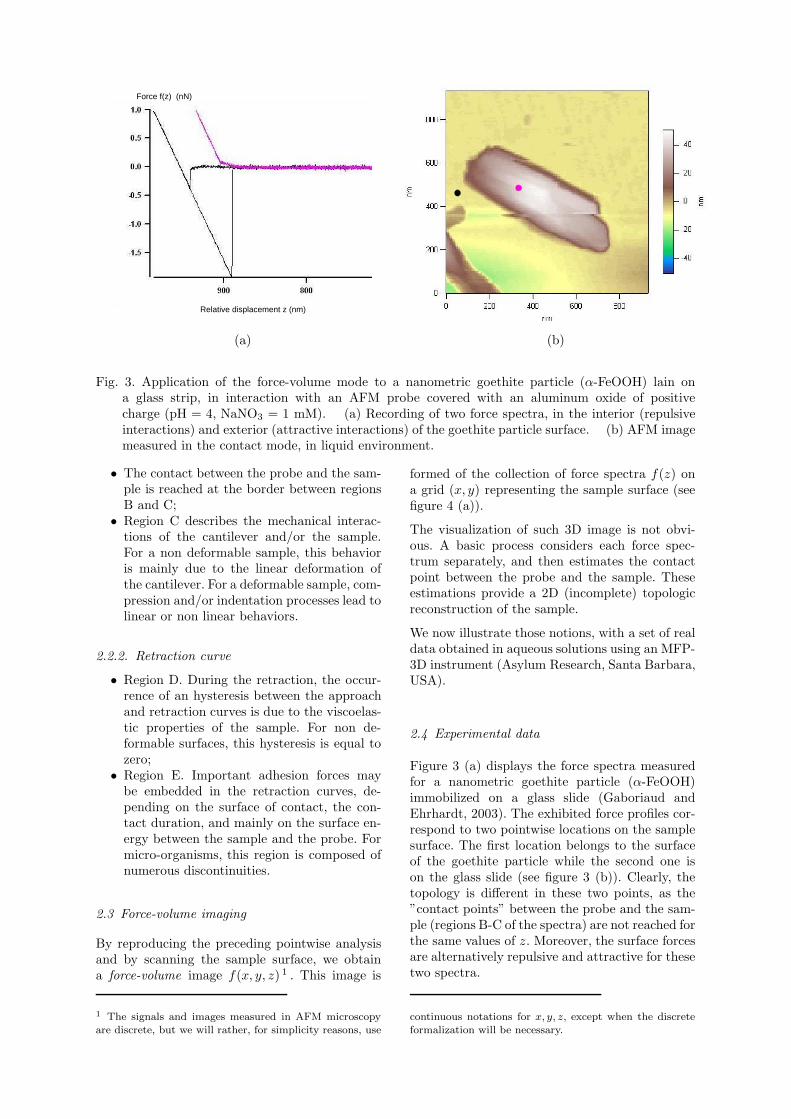
Fig. 3. Application of the force-volume mode to a nanometric goethite particle (α-FeOOH) lain ona glass strip, in interaction with an AFM probe covered with an aluminum oxide of positivecharge (pH = 4, NaNO3 = 1 mM). (a) Recording of two force spectra, in the interior (repulsiveinteractions) and exterior (attractive interactions) of the goethite particle surface. (b) AFM imagemeasured in the contact mode, in liquid environment.

• The contact between the probe and the sam-ple is reached at the border between regionsB and C;

• Region C describes the mechanical interac-tions of the cantilever and/or the sample.For a non deformable sample, this behavioris mainly due to the linear deformation ofthe cantilever. For a deformable sample, com-pression and/or indentation processes lead tolinear or non linear behaviors.

2.2.2. Retraction curve

• Region D. During the retraction, the occur-rence of an hysteresis between the approachand retraction curves is due to the viscoelas-tic properties of the sample. For non de-formable surfaces, this hysteresis is equal tozero;

• Region E. Important adhesion forces maybe embedded in the retraction curves, de-pending on the surface of contact, the con-tact duration, and mainly on the surface en-ergy between the sample and the probe. Formicro-organisms, this region is composed ofnumerous discontinuities.

2.3 Force-volume imaging

By reproducing the preceding pointwise analysisand by scanning the sample surface, we obtaina force-volume image f(x, y, z) 1 . This image is

1 The signals and images measured in AFM microscopy

are discrete, but we will rather, for simplicity reasons, use

formed of the collection of force spectra f(z) ona grid (x, y) representing the sample surface (seefigure 4 (a)).

The visualization of such 3D image is not obvi-ous. A basic process considers each force spec-trum separately, and then estimates the contactpoint between the probe and the sample. Theseestimations provide a 2D (incomplete) topologicreconstruction of the sample.

We now illustrate those notions, with a set of realdata obtained in aqueous solutions using an MFP-3D instrument (Asylum Research, Santa Barbara,USA).

2.4 Experimental data

Figure 3 (a) displays the force spectra measuredfor a nanometric goethite particle (α-FeOOH)immobilized on a glass slide (Gaboriaud andEhrhardt, 2003). The exhibited force profiles cor-respond to two pointwise locations on the samplesurface. The first location belongs to the surfaceof the goethite particle while the second one ison the glass slide (see figure 3 (b)). Clearly, thetopology is different in these two points, as the”contact points” between the probe and the sam-ple (regions B-C of the spectra) are not reached forthe same values of z. Moreover, the surface forcesare alternatively repulsive and attractive for thesetwo spectra.

continuous notations for x, y, z, except when the discrete

formalization will be necessary.

x

y

z

(a) (b)

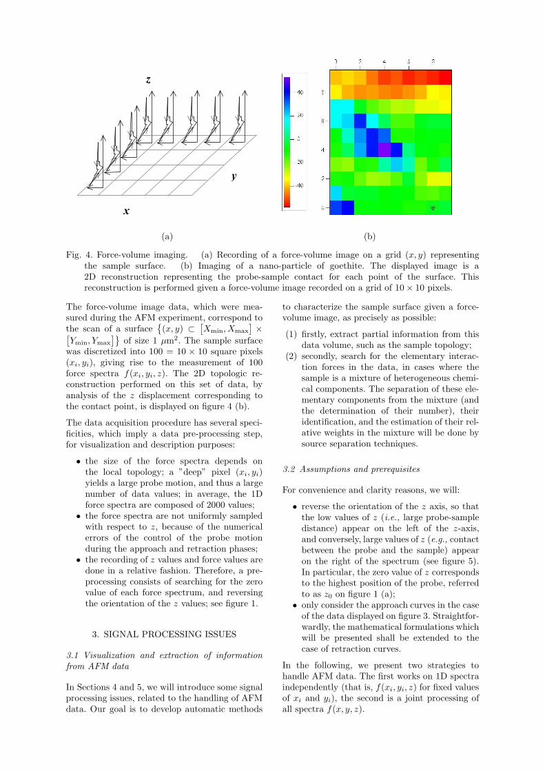
Fig. 4. Force-volume imaging. (a) Recording of a force-volume image on a grid (x, y) representingthe sample surface. (b) Imaging of a nano-particle of goethite. The displayed image is a2D reconstruction representing the probe-sample contact for each point of the surface. Thisreconstruction is performed given a force-volume image recorded on a grid of 10× 10 pixels.

The force-volume image data, which were mea-sured during the AFM experiment, correspond tothe scan of a surface

{(x, y) ⊂

[Xmin, Xmax

]×[

Ymin, Ymax

]}of size 1 µm2. The sample surface

was discretized into 100 = 10 × 10 square pixels(xi, yi), giving rise to the measurement of 100force spectra f(xi, yi, z). The 2D topologic re-construction performed on this set of data, byanalysis of the z displacement corresponding tothe contact point, is displayed on figure 4 (b).

The data acquisition procedure has several speci-ficities, which imply a data pre-processing step,for visualization and description purposes:

• the size of the force spectra depends onthe local topology; a ”deep” pixel (xi, yi)yields a large probe motion, and thus a largenumber of data values; in average, the 1Dforce spectra are composed of 2000 values;

• the force spectra are not uniformly sampledwith respect to z, because of the numericalerrors of the control of the probe motionduring the approach and retraction phases;

• the recording of z values and force values aredone in a relative fashion. Therefore, a pre-processing consists of searching for the zerovalue of each force spectrum, and reversingthe orientation of the z values; see figure 1.

3. SIGNAL PROCESSING ISSUES

3.1 Visualization and extraction of informationfrom AFM data

In Sections 4 and 5, we will introduce some signalprocessing issues, related to the handling of AFMdata. Our goal is to develop automatic methods

to characterize the sample surface given a force-volume image, as precisely as possible:

(1) firstly, extract partial information from thisdata volume, such as the sample topology;

(2) secondly, search for the elementary interac-tion forces in the data, in cases where thesample is a mixture of heterogeneous chemi-cal components. The separation of these ele-mentary components from the mixture (andthe determination of their number), theiridentification, and the estimation of their rel-ative weights in the mixture will be done bysource separation techniques.

3.2 Assumptions and prerequisites

For convenience and clarity reasons, we will:

• reverse the orientation of the z axis, so thatthe low values of z (i.e., large probe-sampledistance) appear on the left of the z-axis,and conversely, large values of z (e.g., contactbetween the probe and the sample) appearon the right of the spectrum (see figure 5).In particular, the zero value of z correspondsto the highest position of the probe, referredto as z0 on figure 1 (a);

• only consider the approach curves in the caseof the data displayed on figure 3. Straightfor-wardly, the mathematical formulations whichwill be presented shall be extended to thecase of retraction curves.

In the following, we present two strategies tohandle AFM data. The first works on 1D spectraindependently (that is, f(xi, yi, z) for fixed valuesof xi and yi), the second is a joint processing ofall spectra f(x, y, z).

5 6 7 8 9 10 11 12

x 10−7

0

2

4

6

8

10

12

14x 10

−8

z

f(z)

8.6 8.8 9 9.2 9.4 9.6 9.8 10 10.2 10.4

x 10−7

−2

−1

0

1

2x 10

−8

z

f(z)

(a) (b)

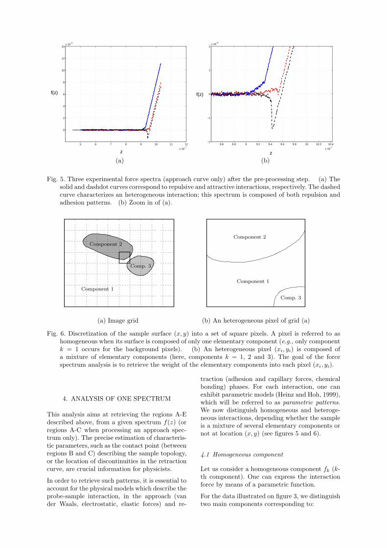
Fig. 5. Three experimental force spectra (approach curve only) after the pre-processing step. (a) Thesolid and dashdot curves correspond to repulsive and attractive interactions, respectively. The dashedcurve characterizes an heterogeneous interaction; this spectrum is composed of both repulsion andadhesion patterns. (b) Zoom in of (a).

Component 1

Comp. 3

Component 2

Component 2

Comp. 3

Component 1

(a) Image grid (b) An heterogeneous pixel of grid (a)

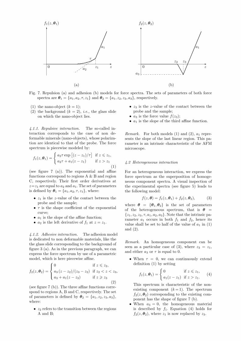
Fig. 6. Discretization of the sample surface (x, y) into a set of square pixels. A pixel is referred to ashomogeneous when its surface is composed of only one elementary component (e.g., only componentk = 1 occurs for the background pixels). (b) An heterogeneous pixel (xi, yi) is composed ofa mixture of elementary components (here, components k = 1, 2 and 3). The goal of the forcespectrum analysis is to retrieve the weight of the elementary components into each pixel (xi, yi).

4. ANALYSIS OF ONE SPECTRUM

This analysis aims at retrieving the regions A-Edescribed above, from a given spectrum f(z) (orregions A-C when processing an approach spec-trum only). The precise estimation of characteris-tic parameters, such as the contact point (betweenregions B and C) describing the sample topology,or the location of discontinuities in the retractioncurve, are crucial information for physicists.

In order to retrieve such patterns, it is essential toaccount for the physical models which describe theprobe-sample interaction, in the approach (vander Waals, electrostatic, elastic forces) and re-

traction (adhesion and capillary forces, chemicalbonding) phases. For each interaction, one canexhibit parametric models (Heinz and Hoh, 1999),which will be referred to as parametric patterns.We now distinguish homogeneous and heteroge-neous interactions, depending whether the sampleis a mixture of several elementary components ornot at location (x, y) (see figures 5 and 6).

4.1 Homogeneous component

Let us consider a homogeneous component fk (k-th component). One can express the interactionforce by means of a parametric function.

For the data illustrated on figure 3, we distinguishtwo main components corresponding to:

zz10

a1

f1(z, θ1)

τ

a2z

a1

f2(z, θ2)

0

a3

z2 z3

(a) (b)

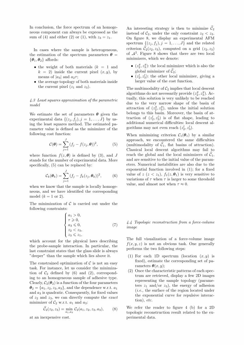
Fig. 7. Repulsion (a) and adhesion (b) models for force spectra. The sets of parameters of both forcespectra are θ1 = {a1, a2, τ, z1} and θ2 = {a1, z2, z3, a3}, respectively.

(1) the nano-object (k = 1);(2) the background (k = 2), i.e., the glass slide

on which the nano-object lies.

4.1.1. Repulsive interaction. The so-called in-teraction corresponds to the case of non de-formable minerals (nano-objects), whose polariza-tion are identical to that of the probe. The forcespectrum is piecewise modeled by:

f1(z, θ1) =

{a2τ exp

[(z − z1)/τ

]if z 6 z1,

a2τ + a1(z − z1) if z > z1

(1)(see figure 7 (a)). The exponential and affinefunctions correspond to regions A & B and regionC, respectively. Their first order derivatives atz=z1 are equal to a2 and a1. The set of parametersis defined by θ1 = {a1, a2, τ, z1}, where:

• z1 is the z-value of the contact between theprobe and the sample;

• τ is the shape coefficient of the exponentialcurve;

• a1 is the slope of the affine function;• a2 is the left derivative of f1 at z = z1.

4.1.2. Adhesive interaction. The adhesion modelis dedicated to non deformable materials, like thethe glass slide corresponding to the background offigure 3 (a). As in the previous paragraph, we canexpress the force spectrum by use of a parametricmodel, which is here piecewise affine.

f2(z, θ2) =

0 if z 6 z2,

a3 (z − z2)/(z3 − z2) if z2 < z < z3,

a3 + a1(z − z3) if z > z3

(2)(see figure 7 (b)). The three affine functions corre-spond to regions A, B and C, respectively. The setof parameters is defined by θ2 = {a1, z2, z3, a3},where:

• z2 refers to the transition between the regionsA and B;

• z3 is the z-value of the contact between theprobe and the sample;

• a3 is the force value f(z3);• a1 is the slope of the third affine function.

Remark. For both models (1) and (2), a1 repre-sents the slope of the last linear region. This pa-rameter is an intrinsic characteristic of the AFMmicroscope.

4.2 Heterogeneous interaction

For an heterogeneous interaction, we express theforce spectrum as the superposition of homoge-neous component spectra. A visual inspection ofthe experimental spectra (see figure 5) leads tothe following model:

f(z, θ) = f1(z, θ1) + f2(z, θ2), (3)

where θ = {θ1, θ2} is the set of parametersof the heterogeneous spectrum, that is θ ={z1, z2, z3, τ, a1, a2, a3}. Note that the intrinsic pa-rameter a1 occurs in both f1 and f2, hence itsvalue shall be set to half of the value of a1 in (1)and (2).

Remark. An homogeneous component can beseen as a particular case of (3), where z3 = z1,and either a3 or τ is equal to 0.

• When τ = 0, we can continuously extenddefinition (1) by setting

f1(z, θ1) =

{0 if z 6 z1,

a1(z − z1) if z > z1.(4)

This spectrum is characteristic of the non-existing component (k = 1). The spectrumf2(z, θ2) corresponding to the existing com-ponent has the shape of figure 7 (b).

• When a3 = 0, the homogeneous materialis described by f1. Equation (4) holds forf2(z, θ2), where z1 is now replaced by z3.

In conclusion, the force spectrum of an homoge-neous component can always be expressed as thesum of (4) and either (2) or (1), with z3 = z1.

In cases where the sample is heterogeneous,the estimation of the spectrum parameters θ ={θ1, θ2} affords:

• the weight of both materials (k = 1 andk = 2) inside the current pixel (x, y), bymeans of |a3| and a2τ ;

• the average topology of both materials insidethe current pixel (z1 and z3).

4.3 Least squares approximation of the parametricmodel

We estimate the set of parameters θ given theexperimental data {(zj, fj), j = 1, . . . , J} by us-ing the least squares method. The estimated pa-rameter value is defined as the minimizer of thefollowing cost function:

C(θ) =

J∑

j=1

(fj − f(zj, θ))2, (5)

where function f(z, θ) is defined by (3), and Jstands for the number of experimental data. Morespecifically, (5) can be replaced by:

Ck(θk) =J∑

j=1

(fj − fk(zj , θk))2, (6)

when we know that the sample is locally homoge-neous, and we have identified the correspondingmodel (k = 1 or 2).

The minimization of C is carried out under thefollowing constraints:

a1 > 0,τ > 0,a3 6 0,z2 < z3,z3 6 z1,

(7)

which account for the physical laws describingthe probe-sample interaction. In particular, thelast constraint states that the glass slide is always”deeper” than the sample which lies above it.

The constrained optimization of C is not an easytask. For instance, let us consider the minimiza-tion of C2 defined by (6) and (2), correspond-ing to an homogeneous sample of adhesive type.Clearly, C2(θ2) is a function of the four parametersθ2 = {a1, z2, z3, a3}, and the dependence w.r.t. a1

and a3 is quadratic. Consequently, for fixed valuesof z2 and z3, we can directly compute the exactminimizer of C2 w.r.t. a1 and a3:

C2(z2, z3) = mina1,a3

C2(a1, z2, z3, a3), (8)

at an inexpensive cost.

An interesting strategy is then to minimize C2

instead of C2, under the only constraint z2 < z3.On figure 8, we display an experimental AFMspectrum {(zj, fj), j = 1, . . . , J} and the related

criterion C2(z2, z3), computed on a grid (z2, z3)of R2. Figure 8 shows that there are two localminimizers, which we denote:

• (zg2 , zg

3): the local minimizer which is also the

global minimizer of C2;• (zl

2, zl3): the other local minimizer, giving a

larger value of the cost function.

The multimodality of C2 implies that local descentalgorithms do not necessarily provide (zg

2 , zg3). Ac-

tually, this solution is very unlikely to be reacheddue to the very narrow shape of the basin ofattraction of (zg

2 , zg3), unless the initial solution

belongs to this basin. Moreover, the basin of at-traction of (zl

2, zl3) is of flat shape, leading to

additional numerical difficulties: local descent al-gorithms may not even reach (zl

2, zl3).

When minimizing criterion C1(θ1) by a similarapproach, we encountered the same difficulties(multimodality of C1, flat basins of attraction).Classical local descent algorithms may fail toreach the global and the local minimizers of C1,and are sensitive to the initial value of the param-eters. Numerical instabilities are also due to theexponential function involved in (1); for a fixedvalue of z (z < z1), f1(z, θ1) is very sensitive tovariations of τ when τ is larger to some thresholdvalue, and almost not when τ ≈ 0.

4.4 Topologic reconstruction from a force-volumeimage

The full visualization of a force-volume imagef(x, y, z) is not an obvious task. One generallyperforms the two following steps:

(1) For each 1D spectrum (location (x, y) isfixed), estimate the corresponding set of pa-rameters θ(x, y);

(2) Once the characteristic patterns of each spec-trum are retrieved, display a few 2D imagesrepresenting the sample topology (parame-ters z1 and/or z3), the energy of adhesion(i.e., the surface of the region located underthe exponential curve for repulsive interac-tion), etc.

We refer the reader to figure 4 (b) for a 2Dtopologic reconstruction result related to the ex-perimental data.

4 5 6 7 8 9 10 11 12

x 10−7

−1

0

1

2

3

4x 10

−9

dataLS solution

0.5

1

1.5

2

2.5

3

3.5

4

4.5

5

5.5

x 10−17

z3

z2

Least square criterion C2(z2,z3)

Region z3<z2

5 6 7 8 9 10

x 10−7

5

6

7

8

9

10

x 10−7

(a) (b)

4 5 6 7 8 9 10 11 12

x 10−7

9

10

x 10−20

z2

Least square criterion C2(z2,z3); z3 is fixed

(c) (d)

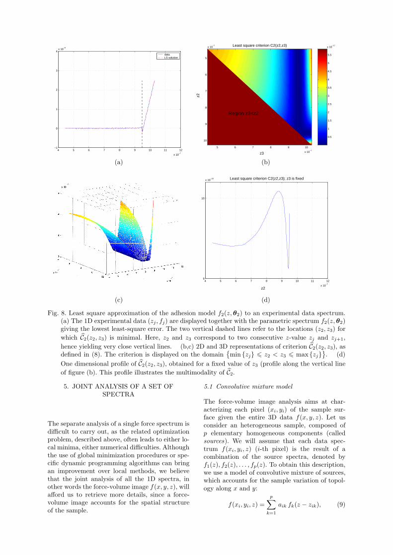
Fig. 8. Least square approximation of the adhesion model f2(z, θ2) to an experimental data spectrum.(a) The 1D experimental data (zj , fj) are displayed together with the parametric spectrum f2(z, θ2)giving the lowest least-square error. The two vertical dashed lines refer to the locations (z2, z3) for

which C2(z2, z3) is minimal. Here, z2 and z3 correspond to two consecutive z-value zj and zj+1,

hence yielding very close vertical lines. (b,c) 2D and 3D representations of criterion C2(z2, z3), asdefined in (8). The criterion is displayed on the domain

{min {zj} 6 z2 < z3 6 max {zj}

}. (d)

One dimensional profile of C2(z2, z3), obtained for a fixed value of z3 (profile along the vertical line

of figure (b). This profile illustrates the multimodality of C2.

5. JOINT ANALYSIS OF A SET OFSPECTRA

The separate analysis of a single force spectrum isdifficult to carry out, as the related optimizationproblem, described above, often leads to either lo-cal minima, either numerical difficulties. Althoughthe use of global minimization procedures or spe-cific dynamic programming algorithms can bringan improvement over local methods, we believethat the joint analysis of all the 1D spectra, inother words the force-volume image f(x, y, z), willafford us to retrieve more details, since a force-volume image accounts for the spatial structureof the sample.

5.1 Convolutive mixture model

The force-volume image analysis aims at char-acterizing each pixel (xi, yi) of the sample sur-face given the entire 3D data f(x, y, z). Let usconsider an heterogeneous sample, composed ofp elementary homogeneous components (calledsources). We will assume that each data spec-trum f(xi, yi, z) (i-th pixel) is the result of acombination of the source spectra, denoted byf1(z), f2(z), . . . , fp(z). To obtain this description,we use a model of convolutive mixture of sources,which accounts for the sample variation of topol-ogy along x and y:

f(xi, yi, z) =

p∑

k=1

aik fk(z − zik), (9)

where:

• coefficient aik is the contribution of the k-thsource at the interior of the i-th pixel;

• functions fk are identical to the functionsf1 and f2 defined in the particular caseof repulsive and adhesive interactions witha non deformable sample. Other types ofinteractions may also occur, namely in thecase of deformable nano-objects and in theretract phase;

• distances zik are homogeneous to probe-sample distances, and characterize the topol-ogy of the k-th source at the interior of thei-th pixel. These parameters are identical toz1 and z3 in (1) and (2).

Clearly, the occurrence of several sources in the in-terior of the same pixel indicates that the chemicalsample is locally heterogeneous (aik 6= 0 for the i-th pixel and for several values of k); see figure 6.

The joint estimation of the sources, their topologyand the mixture coefficients from a force-volumeimage f(x, y, z) can be seen as a source separa-tion problem. It is a classical signal processingproblem, which however, is far to be trivial forconvolutive mixtures.

5.2 Source separation from convolutive mixtures

Equation (9) rereads:

f(xi, yi, z) =

p∑

k=1

aik

(δzik

∗z

fk

)(z), (10)

where δzik(z) = δ(z − zik) represents the 1D

Dirac distribution. Clearly, (10) reduces to theclassical instantaneous linear model encounteredin source separation, when the parameters zik areall equal to zero, i.e., when sample topology isflat. When the topology is not flat, the sourceseparation problem is specially difficult, since thesample topology is unknown, as well as the sourcesand their respective weights in the mixture. Ina formal viewpoint, model (10) is non linearw.r.t. parameters zik. However, the 1D Fouriertransform of f(xi, yi, z) w.r.t. z reads:

f(xi, yi, νz) =

p∑

k=1

aik exp (−2jπνz zik) fk(νz),

(11)denoting by ” . ” the 1D Fourier transform op-erator, and by νz the frequencies along z. Thismodel is now bilinear w.r.t. aik, exp (−2jπνz zik),

and signals fk(νz).

5.3 Inversion of the convolutive mixture model

The inversion of the mixture model amounts toestimating the mixture parameters, i.e., coeffi-

cients aik, zik, and the source signals fk (and theirnumber p) given the experimental data and model(10). It is well known that the source separa-tion problem is an ill-conditioned inverse problem,which suffers from several indeterminacies. In par-ticular, we have:

δzik∗ fk =

(δzik

∗ δ−z′

k

)∗

(δz′

k∗ fk

). (12)

In other words, the sources fk can only be sepa-rated up to a delay z′k.

As seen in section 4, the physical models de-scribing the interactions which occur during themotion of the probe (approach or retraction) areavailable. They provide us with parametric modelsof the source signals fk, also referred to as decom-position into elementary patterns:

fk(z) = fk(z, θk), (13)

where the so-called patterns (discontinuity, expo-nential curve, etc.) embedded into the elementaryspectra are described by the set of parameters θk.

We expect that the use of multilinear tensorfactorization algorithms (Harshman et al., 2003),coupled with this parametric decomposition ofsources, will afford us to solve the problem ofsource separation from convolutive mixtures.

5.4 Accounting for the probe geometry

The model (10) describing the probe-sample forceinteractions is often unrealistic, since it does notaccount for the probe geometry. The latter modelis only valid when the width of the probe is neg-ligible w.r.t. the size of the square pixels (xi, yi)discretizing the sample surface.

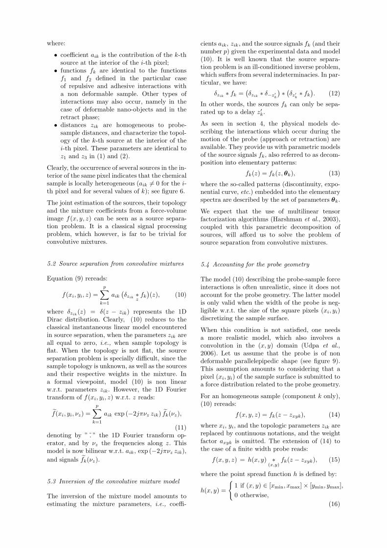
When this condition is not satisfied, one needsa more realistic model, which also involves aconvolution in the (x, y) domain (Udpa et al.,2006). Let us assume that the probe is of nondeformable parallelepipedic shape (see figure 9).This assumption amounts to considering that apixel (xi, yi) of the sample surface is submitted toa force distribution related to the probe geometry.

For an homogeneous sample (component k only),(10) rereads:

f(x, y, z) = fk(z − zxyk), (14)

where xi, yi, and the topologic parameters zik arereplaced by continuous notations, and the weightfactor axyk is omitted. The extension of (14) tothe case of a finite width probe reads:

f(x, y, z) = h(x, y) ∗(x,y)

fk(z − zxyk), (15)

where the point spread function h is defined by:

h(x, y) =

{1 if (x, y) ∈ [xmin, xmax] × [ymin, ymax],

0 otherwise,

(16)

probez

y

x surface of the sample

Fig. 9. Accounting for the probe geometry. Here,the shape of the probe is modeled as a nondeformable parallelepipedic material.

and[xmin, xmax

]×

[ymin, ymax

]stands for the

horizontal cross-section of the probe.

For an heterogeneous sample, we generalize theabove model as follows:

f(x, y, z) = h(x, y) ∗(x,y)

p∑

k=1

[axyk fk(z − zxyk)

].

(17)

When the force-volume image data are finely reso-luted along the (x, y) dimension, we can expect toreconstruct p fine resoluted images representingthe sample topology zxyk (k = 1, . . . , p) and pmaps representing the weights axyk of the ele-mentary components (k = 1, . . . , p). The jointestimation of h and of the mixture parameterscan then be expressed as a deconvolution prob-lem, coupled with a source separation problem. Anatural strategy to cope with it is to process thefollowing three steps:

(1) identify the point spread function h(x, y).This step can be done by means of a learningsequence, corresponding to a mineral flatnano-object lying on a glass slide;

(2) solve the deconvolution problem, and thusremove the effect of h(x, y);

(3) finally, solve the source separation problem(10), in which the probe is of negligiblewidth.

Note that models (15) and (17) may be gener-alized when the probe extremity is not of flatshape. The point spread function h would not onlydepend on (x, y), but also on z to account for therelative depth of the probe extremity.

6. CONCLUSIONS

In this paper, we have briefly introduced the AFMmodalities, and the physical processes which arerelated to the record of force spectra and force-volume images. Firstly, we have exhibited someparametric models describing an homogeneous

component alone by a collection of shape factors(discontinuities of the spectrum, spatial topologyof the component). Secondly, we have introduceda convolutive mixture model describing heteroge-neous interactions, where the mixture model refersto the homogeneous components embedded in agiven pixel, and the convolution operator accountsfor the topology of the elementary components in-side a pixel, and for the probe geometry. We haveillustrated these models with a set of experimentaldata obtained in aqueous solutions using an MFP-3D instrument.

From a signal processing standpoint, future workswill aim at developing advanced methods ded-icated to force-volume images, namely the de-composition of a 1D spectrum into elementarypatterns, the factorization and the deconvolutionof a force-volume image. We believe that thesimultaneous process of all 1D spectra, i.e., ofa force-volume image, will bring more accurateresults than the separate analysis of each 1D forcespectrum. We expect that the use of multilineartensor factorization algorithms, coupled with theparametric description of elementary spectra, willafford us to solve the problem of source separationfrom convolutive mixtures.

ACKNOWLEDGMENT

The authors would like to thank Pr. Jerome Idierfor his helpful comments on the optimization part.

REFERENCES

Binnig, G. (1986). Atomic force microscope andmethod for imaging surfaces with atomic res-olution. US Patent 4(724), 318.

Binnig, G., C. F. Quate and C. Gerber (1986).Atomic force microscope. Physical ReviewLetters 56(9), 930–933.

Butt, H.-J., B. Cappella and M. Kappl (2005).Force measurements with the atomic forcemicroscope: technique, interpretation and ap-plications. Surface Science Reports 59(1–6), 1–152.

Gaboriaud, F. and J.-J. Ehrhardt (2003). Effectsof different crystal faces on surface charge ofcolloidal goethite (a-FeOOH) particles: an ex-perimental and modeling study. Geochimicaand Cosmochimica Acta 67(5), 967–983.

Gaboriaud, F. and Y. F. Dufrene (2007). Atomicforce microscopy of microbial cells: applica-tion to nanomechanical properties, surfaceforces and molecular recognition forces. Col-loids and Surfaces B: Biointerfaces 54, 10–19.

Giessibl, F. J. (2003). Advances in atomicforce microscopy. Review of Modern Physics75(3), 949–983.

Harshman, R. A., S. Hong and M. E. Lundy(2003). Shifted factor analysis – Part I:Models and properties. J. Chemometrics17(7), 363–378.

Heinz, W. F. and J. H. Hoh (1999). Spatially re-solved force spectroscopy of biological sur-faces using atomic force microscope. Trendsin Biotechnology 17(4), 143–150.

Sokolov, I. Y., G. S. Henderson and F. J.Wicks (1999). Force spectroscopy in non-contact mode. Applied Surface Science140(3–4), 358–361.

Udpa, L., V. M. Ayres, Y. Fan, Q. Chen and S. A.Kumar (2006). Deconvolution of atomic forcemicroscopy data for cellular and molecularimaging. IEEE Signal Processing Magazine23(3), 73–83.

Wiesendanger, R. (1994). Scanning Probe Mi-croscopy and Spectroscopy: Methods and Ap-plications. Cambridge Univ. Press, Cam-bridge, MA.