AECL-7244

ATOMIC ENERGY K £ k 3 § L'ENERGIE ATOMIQUEOF CANADA UMITED Y j f t S j r DU CANADA LIMITEE

MULTI VARIABLE CONTROL IN NUCLEAR POWER STATIONS:

OPTIMAL CONTROL

Contrdie multivariable dans les centrales nucleaires:

Contrdie optimal

M. PARENT and P.D. McMORRAN

Chalk River Nuclear Laboratories Laboratoires nucle'aires de Chalk River

Chalk River, Ontario

November 1982 novembre

ATOMIC ENERGY OF CANADA LIMITED

MULT!VARIABLE CONTROL IN NUCLEAR POWER STATIONS:

OPTIMAL CONTROL

by

M. Parent and P.D. McMorran

Chalk River Nuclear LaboratoriesChalk River, Ontario KOJ U O

1982 NevercberAECL-7244

L'ENERGIE ATOMIQUE DU CANADA, LIMITEE

Contrôle multivariable dans les centrales nucléaires:

Contrôle optimal

par

H. Parent et P.D. McMorran

Résumé

Les méthodes multivariables offrent la possibilité d'améliorerle contrôle des centrales nucléaires et autres grandes installations. Lecontrôle optimal linéaire-quadratique est une méthode mult;variable fondéesur la minimisation d'une fonction de coQt. Une technique connexe faitappel au filtre Kalman pour l'estimation de l'état d'une centrale a partirdes mesures de bruit.

On a développé un programme conceptuel pour le contrôle optimalet le filtrage Kalman faisant partie d'un ensemble de conception aidéepar ordinateur pour les systèmes de contrôle multivariable. On décrit ladémonstration de la méthode faite sur une maquette de générateur de vapeurde centrale nucléaire et l'on donne les résultats simulés.

Laboratoires nucléaires de Chalk RiverChalk River, Ontario KOJ 1J0

Novembre 1982

AECL-7244

ATOMIC ENERGY OF CANADA LIMITED

MULTIVARIABLE CONTROL IN NUCLEAR POWER STATIONS:

OPTIMAL CONTROL

by

M. Parent and P.D. McMorran

ABSTRACT

Multi-variable methods have the potential to improve the

con re of large systems such as nuclear power stations.

LJ.II. -quadratic optxmaj. control is a multivariable method

based on the minimization of a cost function. A related

technique leads to the Kalman filter for estimation of plant

state from noisy measurements.

A design program for optimal control and Kalman filtering

has been developed as part of a computer-aided design package

for multivariable control systems. The method is demonstrated

on a model of a nuclear steam generator, and simulated results

are presented.

Chalk River Nuclear LaboratoriesChalk River, Ontario KOj U O

1982 Novembe rAECL-7244

(i)

TABLE OF CONTENTS

Page

LIST OF FIGURES (ii)

NOMENCLATURE (iii)

1. INTRODUCTION 1

2. OPTIMAL CONTROL THEORY . 2

2.1 Optimal Regulator Concept 22.2 The Deterministic Optimal Regulator 52.3 Stochastic Estimation of the State 11

Variables2.4 Kalman-Bucy Filter 132.5 Determination of Cost or Noise 17

Covariance Matrices

3. IMPLEMENTATION IN MVPACK 18

4. EXAMPLE OF A NUCLEAR STEAM GENERATOR 20

4.1 Kalman Filter Design 214.2 Optimal Controller Design 22

5. SUMMARY AND CONCLUSIONS 29

6. REFERENCES 29

(ii)

LIST OF FIGURES

FIGURE 1 Optimal Controller Structure

FIGURE 2 Time-Invariant Optimal Regulator

Page

4

6

FIGURE 3 State-Feedback Controller 8

FIGURE 4 Noisy Plant Model 12

FIGURE 5 Kalman-Bucy Filter 14

FIGURE 6 Comparison of the Responses of the 23Steam Generator Model and theKalman-Bucy Filter to a Steam ValveDisturbance

FIGURE 7 Response of the Optimal Controllerto an Initial Pressure Deviation,with the 6 States Provided by theModel

26

FIGURE 8 Response of the Optimal Controllerto an Initial Pressure Deviationwith the fa States Provided by aKalman Filter Having the CorrectInitial Condition

27

FIGURE 9 Response of the Optimal Controllerto an Initial Pressure Deviationwith the 6 States Provided by aKalman Filter Having IncorrectInitial Conditions

28

(iii)

NOMENCLATURE

In general, capital letters represent matrices, while

lower-case letters are used for vectors and scalars. Following

modern practice, no additional marking is used to identify

vectors or matrices. Such distinction will be clear from the

context.

Symbol Description Defining

Equation

A Plant dynamics matrix (1)

A Reduced model dynamics matrix (27)

B Plant input matrix (1)

B r Reduced model input matrix (27)

C Plant output matrix (2)

C Augmented system output matrix (32)

C Reduced model output matrix (27)

D ' Reduced model input-output direct (27)coupling matrix

F Output terminal cost matrix (3)

H Kalman filter gain matrix (19)

H Reduced Kalman filter gain matrix (27)

I r Identity matrix (rxr) (32)

J Quadratic cost functional (3)

K Optimal controller state-feedback (4)matrix

M State-costate equation matrix (8)

P Riccati matrix-differential (5)equation solution

(iv)

NOMENCLATURE [aontlnand)

Symbol Description Defining~ Equation

PQ Initial state covariance (21)

matrix

Q Output cost matrix (3)

r Order of the reduced model (27)

R Input cost matrix (3)

t Time

t Initial time of observation (18)

T Terminal time (3)

u Plant input vector (1)

,Vn,,V, ,,V0, Partitions of the eigenvector (12)1Z Zl ££ m a t r i x Of M

x Plant state vector (1)

x Initial state mean

x State vector estimate (18)

xr Reduced state vector estimate (27)

x* Costate vector (7)

y Plant output vector (2)6 Small perturbation from

nominal value

6 Output noise vector (17)

9 Output noise covariancematrix

A Positive block of the diagonal (12)eigenvalue matrix of M

(v)

NOMENCLATURE {continued)

Symbol Description DefiningEquation

£ Input noise vector (16)

H Input noise covariance matrix

T Reversed time (T-t) (9)

SUPERSCRIPTS

-1 Matrix inverse

T Matrix transpose

1. INTRODUCTION

Multivariable methods have the potential to improve

the control of large systems such as nuclear power stations.

The complexity of nuclear power stations requires careful

analysis of the roles and interactions of plant variables

to determine the appropriate control strategy and to meet

engineering specifications. Conventional single-variable

methods are customarily used, but they lead to a difficult

and empirical design procedure, previous developments have

shown that multivariable techniques can deal with such complex

problems. For this reason, MVPACK [1], a computer-aided design

package for multivariable controllers, is being developed in

the Dynamic Analysis Laboratory at the Chalk River Nuclear

Laboratories. This report presents the theory and computer

implementation of linear-quadratic optimal control. Extensive

theoretical development and successful application in the aero-

space industry proves the maturity of this technique and

motivates this study.

Optimal control is a state-space multivariable method

based on the time response of the system. Its objective is to

optimize the trajectory of the plant according to a performance

index given by the designer. This index must take into account

engineering and economic constraints to ensure safe and efficient

operation of the plant. Optimal control theory handles two

families of problems; the deterministic optimal controller, and

the stochastic state estimator or Kalman-Bucy filter. Both are

part of the optimal control problem encountered in practical

situations. There are several forms of optimal controller, of

which the most important is the optimal regulator that tries to

keep the plant close to a constant reference.

This report presents the theory of the optimal deterministic

regulator and the steady-state Kalman-Bucy filter. It describes

- 2 -

the implementation of the corresponding module MVOPT within

MVPACK. The technique is illustrated on the control of a

steam qenerator.

2. OPTIMAL CONTROL THEORY

This section presents the mathematical theory used for the

development of the optimal control design module MVOPT. We do

not attempt to give any new results in optimal control but

simply define the problem and present the solution method used.

The notation is that adopted earlier [2] for the development of

MVPACK.

The general problem of optimal control is to find an input

signal such that the response of a given plant minimizes a

specified criterion, or cost function. A wide range of problems

fit this definition, some of which have been covered by Athans

and Palb 13]. However, in this report, we present only the •

special case of a linear system with a quadratic criterion, sub-

jected to Gaussian noise [4]. in this case, the optimal input

is a linear function of the process state, and the result is a

state-feedback controller. This special problem is of importance

because it applies to the regulation of any system to a constant

reference condition.

2.1 Optimal Regulator Concept

The linear-quadratic Gaussian optimal control problem can

be decomposed into two associated problems using the separation

theorem [4]. These are:

- deterministic idral response analysis anu design,

- stochastic estimation analysis and design.

- 3 -

Then, the complete solution of the stochastic feedback control

problem is obtained by combining the results of the first two

steps. This section deals with the deterministic optimal

control case where input, state, and output variables are

assumed to be measured exactly.

The first step in optimal control strategy is to

determine the desired trajectory the plant must follow. This

ideal trajectory can be obtained by experience, coupled with

computer simulation or as the result of a preliminary optimization.

It is chosen to meet economic, safety and engineering require-

ments on plant operation. However, due to disturbances and

modeling approximations., the corresponding ideal input cannot

drive the actual plant along the ideal trajectory. Thus, a

feedback structure is required as shown in Figure 1. The

resulting input causes the plant to follow the ideal trajectory

with acceptable accuracy during the time interval of interest.

The deterministic optimal control problem is to find the feed-

back controller such that a quadratic functional of input and

state deviations is minimized. This insures that the plant

follows the desired trajectory within a certain margin and with

limited control action.

The solution is analytically provided by the minimum

principle of Pontryagin [3] and is given as a state feedback

gain matrix. Provided that the trajectory is known in advance,

the general optimal controller is a time-varying feedback matrix

to be precomputed. So the resulting controller can be very

complex. However, this theory provides simple solutions in

certain practical cases such as the optimal regulator.

The optimal regulator is defined as a restriction of

the optimal controller in which the reference trajectory is

constant. In normal operation, a power station is characterized by:

NOMINALINPUT

(\

Su(t) '

CONTROLCORRECTION

b u(t) y¥ ACTUAL

INPUT

IDEAL COMPUTED

TRAJECTORY

PLANT

CONTROLLER

x(t) >6ACTUAL K

STATE

NOMINALSTATE

x B ( t )

98x(t)

STATEPERTURBATION

FIGURE 1: OPTIMAL CONTROLLER STRUCTURE

- 5 -

- constant or slowly varying reference compared to the

dynamics of the plant,

- time interval of interest large compared to the

time-response of the plant.

Then, a regulator can be used to keep the plant close to the

reference given by the overaM power control mechanisms.

Specifically, if we assume that

- the reference is constant, and

- the time interval of interest is infinite,

the resulting optimal controller i s a constant feedback-gain

matrix. This is the deterministic, time-invariant optimal

regulator presented in the next section.

2.2 The Deterministic Optimal Regulator

The optimal regulator structure is derived from Figure 1

but with constant ideal references obtained from the complete

model of the plant. The linearized plant is time-invariant

while its state remains near the operating point. For each

specific operating point, the optimal regulator can be

scheduled to be a time-invariant regulator as shown in Figure 2.

All variables are now represented as perturbations from the

reference values, so the regulator always attempts to drive the

state to zero.

The plant is described by the linearized perturbation model

[4]

^ x(t) = Ax(t) + Bu(t) (1)

y(t) = Cx(t) (2)

u(t)B — >

11 s

A

<REGULATOR

<

x ( t )C

y ( t )

FIGURE 2: TIME - INVARIANT OPTIMAL REGULATOR

- 7 -

where

x is the state vector, of dimension n,

u is the input vector, of dimension p,

y is the output vector, of dimension m,

A,B and C are constant matrices of appropriate dimensions.

The matrices A, B and C are obtained by linearizing about the

operating point, and x, u and y represent deviations from the

operating point. The optimal regulator is designed to minimize

the quadratic cost functional

J = yT(t}Fy(t) +f [yT(t)Qy(t) + uT(t)Ru(t)]dt (3)J o

where

F is a positive-semidefmite, symmetric-output terminal

cost matrix,

Q is a positive-semidefinite, symmetric-output cost matrix,

R is a positive-definite, symmetric-input cost matrix,

T is the terminal time.

J is such that F and Q become state cost matrices if the plant

output matrix C is replaced by the identity matrix.

The solution to this central problem is the state-feedback

controller shown in Figure 3, with

K(t) = R-^PCt) (4)

where P(t) is the symmetric, positive-definite solution of the

Riccati matrix-differential equation

REF ^ .

rK

uB

ri

i -

A

X

c

HGURE 3: STATE - FEEDBACK CONTROLLER

- 9 -

|-P = -PA - ATP - CTQC + PBR'^P (5)at '

with the terminal condition

P(T) = CTFC (6,'

However, the matrix P can be also obtained by solution of the

reversed-time state-costate equation [5]

CrC)where

/ -A BR - 1B T

(8)

CXQC A1

and

T = T - t (9)

The terminal condition of equation (6) becomes the initial

condition

x*(0) = CTFCx(0) (10)

Then, P(T) is such that

X*(T) = P(T)X(T) . (11)

for all T.

- 10 -

The matrix P(x) can then be found from a modal analysis

of M [5,6,7]. M is a Hamiltonian matrix [6] so the eigen-

values are symmetric with respect to the imaginary axis, and

this modal decomposition can be written

V12 >

(12)I \ /\ I

V21

The eigenvector matrix is partitioned into four nxn blocks

such that the first n columns are the eigenvectors cor-

responding to A, the diagonal matrix of right half-plane

eigenvalues. If the matrix M does not have 2n independent

eigenvectors, the modal decomposition can be replaced by the

Jordan canonical form of M [7, pg. 323]. The resulting solution

can be obtained in a form such that it involves only real matrices

and negative exponentials, so it is stable for large values of x.

As discussed in Section 2.1, for a regulator it is appro-

priate to let the time interval T be infinite. Then, the cost

functional becomes

[xT(t)Qx(t) + uT(t)Ru(t)]dt (13)

and the matrix P appearing in the feedback matrix K is constant.

P is obtained as the infinite-time limit of the negative exponen-

tial solution of the Riccati matrix differential equation [5]

p =

Then, the solution is a time-invariant regulator with the

state-feedback matrix

(15)

- 11 -

Two properties of the optimal regulator obtained can

be pointed out:

(i) The modes of the closed-loop optimal regulator

are the left half-plane eigenvalues of the matrix M

and the eigenvector matrix is V., [7].

(ii) The quadratic criterion reduces the higher order

terms [4] in the Taylor series expansion used to

linearize ths plant. Thus, the linear model

approximation is kept "honest".

2.3 Stochastic Estimation of the State Variables

The stochastic estimation problem is approached in this

report because of its complementarity and duality with deter-

ministic optimal control. As shown in the previous sections,

optimal control theory generates state-feedback controllers.

However, with the high-order models required to describe complex

systems, the state vector cannot be measured completely and

exactly. Indeed, some of the state variables are not directly

measurable and noise often corrupts sensor information. Then,

the state vector must be optimally estimated to complete the

optimal controller.

An estimator produces a state vector estimate using

plant input and output information. To design this stochastic

estimator, the plant is modeled as shown in Figure 4. The

vector 5 can be used to model parameter uncertainty while the

vector 6 models instrumentation noise. Once the plant model

is linearized at the current setpoint, it is described by the

linear equations

g£x(t) = A(t)x(t) +B(t)(u(t) + Ut)) (16)

y(t) = C(t)x(t) + 8(t) (17)

- 12 -

A

> -

orCJ3

- 13 -

For the development of the theory, the following assumptions

are made:

- The initial sta:~e vector is Gaussian with known mean

x and covariance P .o o

- £ and 6 are independent white Gaussian noise vectors

with zero mean and known covariance matrices ~(t) and

9(t), respectively. H(t) is symmetric positive semi-

definite, and 0 (t) is symmetric positive definite.

- The plant matrices A, B and C are deterministic

and known.

The stochastic estimation problem is to find an estimate

x(t) of the true state vector x(t) which is optimal in a given

statistical sense. The Kalman-Bucy filter provides such an

estimate satisfying simultaneously various criteria such as

least squares, minimum variance and maximum likelihood. This

filter is presented in the next section and is used in steady-

state form to complete the optimal regulator.

2.4 Kalman-Bucy Filter

The structure of the optimal filter is shown in Figure 5.

The optimal estimate x is generated by

grjr x = Ax + Bu + H(y-Cx) ;x(tQ) = xQ (18)

where t is the initial time, and the filter gain matrix H

is given by

H(.t) = P(t)CT(t) 6-1(t) (19)

PLANTMEASUREMENT

V *H

\

1T1 s

A

c

AX

FIGURE 5: KALMAN - BUCY FILTER

- 15 -

P(t) is the positive definite solution of the Riccati matrix

differential equation

££- P(t) = AP + PAT + BHBT - PC T O^CP (20)

with the initial condition

P(tQ) = PQ (21)

where PQ is the covariance matrix of x(t Q).

The Riccati equation (20) may be solved by exploiting

duality with the optimal regulator. If the Riccati equation (5)

for the regulator is rewritten for r=T-t, it becomes

g— P = A TP + PA + CTQC - P B R " ^ ? (22)

and comparison of equations (20) and (22) shows that

/ T T i

/ -A1 cre-'cM =1 ) (23)

\ T\BHBX A

corresponds to the regulator state-costate matrix. The

initial condition is

= Pox(tQ) (24)

and, as before, P(t) satisfies

x*(t) = P(t)x(t) (25)

This analogy may he verified by substituting equations (25)

and (23) into equation (7), with T replaced by t, to obtain

- 16 -

the filter Riccati equation (20). Thus, the Kalman-Bucy

filter in forward time is analogous to the optimal controller

in reversed time.

As in the case of the optimal controller, the general

solution of this problem is complex and time-varying. However,

in practical applications it is possible to use a steady-state

Kalman-Bucy filter. In this case, the following assumptions

are made:

- The linear model of the plant is time-invariant, so

A, B, C are constant matrices.

- Noise statistics are stationary, so 5 and 9

are constant matrices.

- The initial time of observation t is far in the

past, so t -»• -«>.

These assumptions are valid for a plant that follows a constant

or slowly varying reference as in the regulator case. Then

the matrix P of the filter is obtained as the infinite-time

limit of the negative exponential solution of equation (2 0).

This solution has been presented for the time-invariant

optimal regulator. So, the steady-state Kalman-Bucy filter

is time-invariant and precomputable with a filter gain matrix

H

The important properties of the Kalman-Bucy filter are:

- The deterministic optimal controller, combined with

the Kalman-Bucy filter, produces the optimal control

correction in the mean-square sense.

- 17 -

- The modes of this filter are only excited by the

noise [1, pg. 59] .

- The modes of the combined closed-loop system, including

the Kalman-Bucy filter and the deterministic optimal

controller, are those of the plant with state feedback

(eigenvalues of A-BK) and those of the open-loop filter

(eigenvalues of A-HC) [4]. Thus, the closed-loop

system is stable.

2.5 r ̂ termination of Cost or Noise Covariance Matrices

In the optimal controller the role of the cost matrices

is to weight the deviations of the variables from the ide.."

trajectory However, it is usually impossible to trans]: -•>

engineering specifications into a quadratic form. Moreot-fc-

no rule can be defined to choose these costs. So, tiieir

determination relies mainly on experience and is based on a

trial procedure that aims to achieve acceptable dynamic response.

One means of assessing the dynamics is to examine the positions

of the closed-loop poles.

In the Kalman-Bucy filter, the noise covariance matrices

model plant uncertainties. 6 can be associated with output

measurement noise and E with parameter uncertainties. Again,

determination of these matrices is a difficult problem which

the designer must solve empirically.

For given cost and covariance matrices, the separation

theorem states that the complete controller-estimate_• is

optimal in the least-square sense. However, it has been shown

that the deterministic optimal controller and the Kalman-Bucy

filter should not be designed independently 18]. In any case,

the design will be initiated with arbitrary cost and noise

- 18 -

covariance matrices. A common way to begin the regulator

design is to fix deviations Sx • or 6u• for each variable

involved in the cost. Then the corresponding diagonal cost

term will be l/6xi or l/6u.. Further adjustment of the cost

can be made using the result of a modal analysis or simulation.

If some engineering specifications are given, such as the

response time or overshoot percentage of a variable, the factor

weighting that variable can be used to meet the requirements.

3. IMPLEMENTATION IN MVPACK

MVPACK [1] is a multivariable control design package

being developed in the Dynamic Analysis Laboratory at CRNL.

It is an interactive system of computer programs running on a

PDP-11/45 minicomputer. MVOPT is the optimal controller and

Kalman-Bucy filter design program, based on the theory presented

in this report.

MVOPT accepts a linear state-space model written in

standard form. Cost or noise covariance matrices may be read

from a file, or entered interactively. MVOPT solves the steady-

state matrix Riccati equation using the eigenvectors of the

state-costate matrix M, as presented above. The necessary

eigenanalysis is performed by the MVEIG moduxe of MVPACK. The

controller or filter generated is the steady-state time-infinite

version.

A second module, MVOPTA, is also available as an aid to

optimal control design. It is a fast and interactive module

that simply computes the modes of the closed-loop controller

corresponding to the cost or noise covariance matrices chosen.

It is used to accelerate the iterative process of choosing

weights using the eigenvalues of the controlled plant as a

decision criterion.

- 19 -

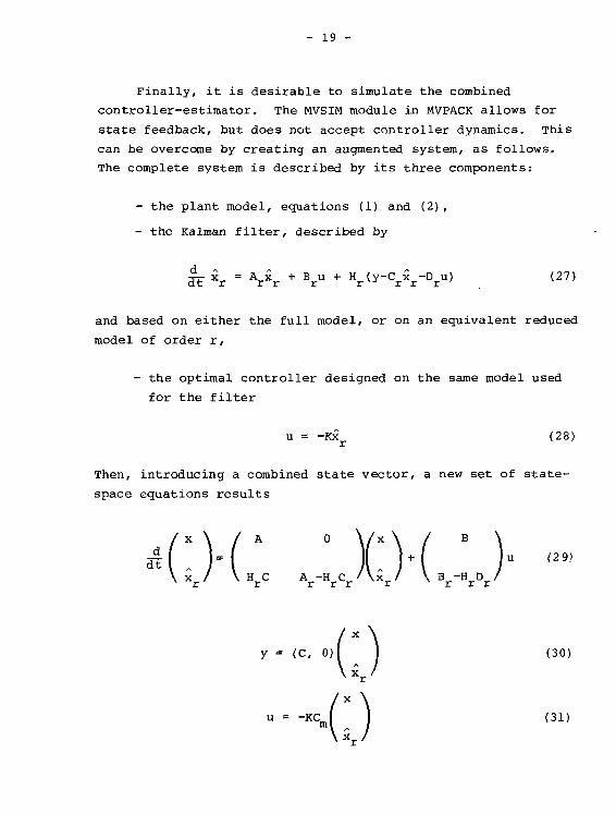
Finally, it is desirable to simulate the combined

controller-estimator. The MVSIM module in MVPACK allows for

state feedback, but does not accept controller dynamics. This

can be overcome by creating an augmented system, as follows.

The complete system is described by its three components:

- the plant model, equations (1) and (2),

- the Kalman filter, described by

WE *r = Ar*r + Br U + Hr(y-Crxr-Dru) (27)

and based on either the full model, or on an equivalent reduced

model of order r,

- the optimal controller designed on the same model used

for the filter

u = -Kxr (28)

Then, introducing a combined state vector, a new set of state-

space equations results

Mxr/ \ HrC

y = (c, 0)1 1 (30)

u = -Kcl J (31)

- 20 -

with

Cm = (0, Ir) (32)

The D u term in equations (27) and (2 9) is required if such

a term appears in the output equation of the reduced model.

The MVOSIM module is provided to generate these matrices, per-

mitting simulation using MVSIM.

4. EXAMPLE OF A NUCLEAR STEAM GENERATOR

Optimal control of a nuclear steam generator is used as

an example to demonstrate the application of the design tool

developed in the preceding sections. This steam generator [9]

is modeled as a 15th-order linear system. No attempt has been

made to produce a 15th-order optimal controller. Instead, a

6th-order reduced model [10] was used for filter and controller

design. Then, the controller was tested on the complete model

to establish both the accuracy of the reduced model and the

efficiency of the optimal controller.

The 6th-order reduced model involves the following state

variables:

x. - Downcomer level

x, - Steam pressure

x, - Downcomer temperature

x4 - Steam quality in the riser

x 5 - Length of subcooled region on the secondary side

x6 - Tube metal temperature of 4th lump, in 4-lump model

where only x. arc; x 2 are accessible to measurement. The state

matrices of the reduced model are [10]

- 21 -

-0

-0

0

4.

0

-0

,053

.143

.0019

6x10-"*

.055

.108

-0

-0

0

6.

0

0

B

.0026

.293

.0084

1x10""

.027

.009

I1'/-62

•[.:•Li.\ 4 .

0.

0.

-0.

-0.

-0.

0.

27

.2

518

030

59

94

0067

332

080

005

188

549

0

1

-1

-0

-0

1

-15.88-P.258

-5.84

-0.309

0.113

-0.588

.672 \

.92

.085

.0013

.059

.63 /

0.

-0.

-0.

-0.

-0.

1.

034089

0029

022

813

44

0.018

0.887

0.0072

4.7x10

-0.008

-0.847

(34)

(33)

C = (35)

D =0.413

.-0.132

(36)

4.1 Kalman Filter Design

The Kalman-Bucy filter was designed on the 6th-order

reduced model. For simulation, the plant was considered free

of output noise. So, the actual role of the filter, once

implemented on the complete model, is to produce an estimate

of the 6 desired state variables, filtering the inaccuracies of

the reduced model. The noise covariance factors were chosen

using MVOPTA with the aim of obtaining filter dynamics that

are faster than the expected dynamics of the optimal controller.

Since 8 must be nonsingular, a small amount of output noise was

assumed.

- 22 -

The filter parameters finally chosen were

H = diag(103, 103, 106, 106, 106, 10s)

0 = diagd, 1)

The resulting gain matrix is

(37)

(38)

H =

/2.0978

53.823

850.10

-13.659

289.92

V7 97.08

180.63 i

2.0978

48.931

-996.37

8.5383

-0.78672/

(39)

and the filter eigenvalues are -0.2511, -1.743, -26.92+jl5.01,

-90.51±j87.70.

A simulation of this filter for estimating the 6 desired

state variables from the output of the 15th-order model is

shown in Figure 6, where each variable is plotted with its

estimate. The test disturbance is a trapezoidal pulse in

steam valve position.

4.2 Optimal Controller Design

The controller was also designed on the 6th-order reduced

model. The value of MVOPTA for controller design was found very

limited, at least in this case. Indeed, MVOPTA gives no indi-

cation of the gains required, and one must know the desired

poles a priori. So, the main tool used in selecting the cost

factors was simulation of the reduced model with its deterministic

controller.

- 23 -

SteamValveLift

DowncomerLevel(m)

0.2

0.1

0.0

-0.11 I 1 1 1 1

•

-

1

SteamPressure(kPa)

DowncomerTemperature

80

1 15th-order model, representing actual process

Estimated by 6th-order Kalman-Bucy filter

FIGURE 6a COMPARISON OF THE RESPONSES OF THE STEAM GENERATORMODEL AND THE KALMAN-BUCY FILTER TO A STEAM VALVEDISTURBANCE

- 24 -

SteamQuality

SubcooledLength(m)

-

0

0

-0

-0

0. 4

0. 2

0.0

0. 2

.05

.00

.05

.10

TubeMetal

TemperatureCO

0.0

-0.4

-0.6

15th-order model, representing actual process

Estimated by 6th-order Kalman-Bucy filter

FIGURE 6b COMPARISON OP THE RESPONSES OF THE STEAM GENERATORMODEL AND THE KALMAN-BUCY FILTER TO A STEAM VALVEDISTURBANCE

- 25 -

The weighting factors finally selected are a reasonable

compromise between the dynamics of the states and the control

actions. The chosen cost matrices are

Q = diag(6, 0.4, 0.04, 0.04, 0.04, 0.04) (40)

R = diagUO1*, 101*)

and the resulting state-feedback matrix is

r-9.92x10"" -3.43X10"3 -3.82xlO"3 0.212 -8.95xlCT3 -2.22xlCT3 JI (42)

The closed-loop poles of the reduced model with this controller

are -1.63xl0"2, -7.06xl0~2, -0.363±jO.044, -0.902+j0.249. When

this controller is applied to the full model, the first 8 poles

are -1.63xlO~2, -7.05xl0~2, -0.362 +jO. 044 , -0.901±jO.249, -1.32,

-1.43. The effect of the controller on the full model is almost

identical to its effect on the reduced model. The remaining

plant poles remain to the left of the controlled poles.

The controller was simulated with constant setpoints and

an initial pressure deviation of 480 kPa (70 psi). The con-

troller must then act to restore the pressure. Figure 7

shows the inputs and outputs for the deterministic case, in

which the 6 states required are known exactly. The same

transient is shown in Figure 8, but the states are obtained

from the 6th-order Kalman filter. The response is close to

the deterministic case, though the feedwater flow (u,) shows

the effect of inaccurate estimation. For this run, the filter

was initialized with the actual initial state, including the

pressure deviation. In practice, such a deviation would result

from an unknown disturbance, and the filter initial state

would be 0. This case is shown in Figure 9. The output response

- 26 -

SteamPressureCkPa)

DowncomerLevel(m)

SteamValveLift

FeedwaterFlow(%)

2

1

1

0

. 0

. 5

. 0

. 5

I 1 1 1 1 1

20 40Time (s)

60 80

FIGURE 7 RESPONSE OF THE OPTIMAL CONTROLLER TO AN INITIALPRESSURE DEVIATION, WITH THE 6 STATES PROVIDEDBV THE MODEL

- 27 -

SteamPressure

(kPa)

DowncomerLevel(m)

SteamValveLift

FeedwaterFlow

80

FIGURE 8 RESPONSE OF THE OPTIMAL CONTROLLER TO AN INITIALPRESSURE DEVIATION WITH THE 6 STATES PROVIDED BYA KALMAN FILTER HAVING THE CORRECT INITIALCONDITION

- 28 -

SteamPressure

(kPa)•2 00

0.0

Downcomer -0.1Level(m) _ 0 - 2

-0. 3

SteamValveLift(*)

Feeciwa terFlow

-30

20 40

Time (s)

60

FIGURE 9 RESPONSE OF THE OPTIMAL CONTROLLER TO AN INITIALPRESSURE DEVIATION WITH THE 6 STATES PROVIDED BYA KALMAN FILTER HAVING INCORRECT INITIAL CONDITIONS

- 29 -

is essentially unchanged, but the feedwater flow now goes

sharply negative initially, as it is acting on incorrect

information. This transient is governed by the 4 s dominant

filter time constant.

These results demonstrate the potential of state-space

methods to generate practical controllers having new structures.

5. SUMMARY AND CONCLUSIONS

The state-of-the-art of linear-quadratic optimal control

theory is summarized in this report, and this method has been

developed into an efficient program module for the design of

optimal controllers. The module, called MVOPT, is now an

operational part of th <3 overall MVPACK program. MVOPT, in

conjunction with model reduction, is used iteratively as a

controller design tool. However, the method is limited by

sensitivity to model accuracy, and there is no guarantee on

the final result if the model is not accurate enough.

6. REFERENCES

[1] P.D. McMorran, "Development of Multivariable Methods

for Plant Control", paper presented at the Seventh

Symposium on Reactor Dynamic Simulation and Nuclear power

Station Control, Montreal, 1980 May.

[2] P.D. McMorran, "Multivariable Control in Nuclear Power

Stations - Survey of Design Methods", Atomic Energy of

Canada Limited, AECL-6583, 1979 December.

[3] M. Athans and P.L. Falb, "Optimal Control", McGraw-Hill,

New York, 1966.

- 30 -

[4] M. Athans, "The Role and Use of the Stochastic Linear-

Quadratic-Gaussian Problem in Control System Design",

IEEE Transactions on Automatic Control, AC-16, pp. 529-552,

1971 December.

[5] D.R. Vaughan, "A Negative Exponential Solution for the

Matrix Riccati Equation", IEEE Transactions on Automatic

Control, AC-14, pp. 72-75, 1969 February.

[6] O.H.D. Waiter, "Real-matrix Solutions for the Linear

Optimal Regulator", Proc. IEE, 119, pp. 621-624, 1972 May.

[7] H. Kwakernaak and R. Sivan, "Linear Optimal Control Systems",

Wiley-Interscience, New York, 1972.

[8] J.M. Mendel, "On the Need for and Use of a Measure of

State Estimation Errors in the Dasign of Quadratic Optimal

Control Gains", IEEE Trans. Auto, Control, AC-16, pp. 500-

503, 1971 October.

[9] P.D. McMorran and T.A. Cole, "Multivariable Control ±-\

Nuclear Power Stations: Modal Control", Atomic Energy

of Canada Limited, AECL-6 690, 1979 December.

[10] M. Parent and P.D. McMorran, "Multivariable Control in

Nuclear Power Stations: Model Order Reduction", Atomic

Energy of Canada Limited, Ai,CL-7 24 5, report in preparation.

ISSN 0067 - 0367

To identify individual documents in the series

we r3ve assigned an AECL- number to each.

Please refer to the AECL- number when re-

questing additional copies of this document

from

Scientific Document Distribution OfficeAtomic Energy of Canada Limited

Chalk River. Ontario, CanadaKOJ 1J0

ISSN 0067 - 0367

Pour identifier les rapports individuels faisantpartie de cette seVie nous avons assign^un nume>o AECL- a chacun.

Veuillez faire mention du numero AECL- sivous demandez d'autres exemplaires de cerapport

Service de Distribution des Documents Otficiels

L'Energie Atomique du Canada LimiteeChalk River, Ontario. Canada

KOJ 1JO

Price $3.00 per copy Prix $3.00 par exempNire

© ATOMIC ENERGY OF CANADA LIMITED, 1982

3268-82