Embed Size (px)
Citation preview
NASA Contractor Report 3410
Atmospheric Studies Related to Aerospace Activities and Remote Sensing Technology
N. D. Sze, R. G. Isaacs, M. Ko, and M. B. McElroy
CONTRACT NASl-15943 MARCH 198 1
,, NASA :. CR 34 10 c-1
https://ntrs.nasa.gov/search.jsp?R=19810011155 2018-06-17T02:04:23+00:00Z
TECH LIBRARY KAFB. NM
NASA Contractor Report 3410
Atmospheric Studies Related to Aerospace Activities and Remote Sensing Technology
N. D. Sze, R. G. Isaacs, M. Ko, and M. B. McElroy Atmospheric attd Environmental Research, Inc. Cambridge, Massachsetts
Prepared for Langley Research Center under Contract NASl-15943
National Aeronautics and Space Administration
Scientific and Technical Information Branch
1981

I”
I
TABLE OF CONTENTS
Page
1. INTRODUCTION ............ T .... 1
2. .MODEL SENSITIVITY STUDIES ... : ......... 3
2.1 Overview ............... t ... ., ., 3
2.2 Model Results ........... : ... 5
2.3 Perturbation Studies ..... T ....... 9
2.4 Concluding Remarks ............ 21
3. TWO-DIMENSIONAL ZONAL MEAN MODELING ...... 22
3.1 Background ................ 22
3.2 Eulerian Mean Model ........... 28
3.3 Generalized Lagrangian Mean (GLM) Zonal Models ............... 36
3.4 Concluding Remarks ............ 42
4. REMOTE SENSING ................ 45
4.1 Background ................ 45
4.2 Role of Earth Curvature and Scattering in Diurnal Photo- chemical Modeling ............ 47
4.3 Optical Paths in a Spherical Shell Atmosphere ................ 49
4.3.1 Geometric Considerations ..... 49
4.3.2 Air Mass Factor Formulation .... 50
4.3.3 The Chapman Function ....... 52
4.3.4 Other Analytical Treatments .... 56
4.3.5 Numerical Forms (including refractive effects) ........ 57
4.3.6 Summary .............. 61
4.4 Treatment of Multiple Scattering in the Spherical Shell Geometry ....... 63
4.4.1 The General Problem ........ 63
4.4.2 Locally Plane-Parallel Approximation ........... 65
4.4.3 Method of Solution ........ 67
4.4.4 Single Scattering Results ..... 72
4.4.5 Multiple Scattering Results .... 81
iii
4.5 Application to Diurnally Dependent Photodissociation Rates . . . . . .
4.6 Diurnal Calculations . . . . . . .
4.6.1 Role of Sphericity . . . . .
4.6.2 Role of Molecular Scattering
4.7 Implications for Remote Sensing . .
5. SUMMARY AND RECOMMENDATIONS . . . . . .
5.1 Model Sensitivity Studies . . . . .
5.2 Two-Dimensional Zonal-Mean Modeling
5.3 Remote Sensing. . . . . . . . . . .
. . . .
. . . .
. . . .
. . . .
. . . .
. . . .
. . . .
. . . .
. . . .
Page
86
90
93
94
95
101
101
102
102
APPENDIX A - Earth-Sun Geometry . . . . . . . . 104
APPENDIX B - Procedure for Refracted Air Mass Calculation . . . . . . . . . 107
APPENDIX C - Integral Quadrature Technique . . . 110
APPENDIX D - Numerical Procedure for Diurnal Calculation . . . . . . . . 114
APPENDIX E - Initialization of Lagrangian Trajectory . . . . . . . . . . . . 117
APPENDIX F - High Altitude Aircraft Emissions . . . . . . . . . . . . . 120
REFERENCES . . . . . . . . . . . . . . . . . . . 124
iv
1. INTRODUCTION
This report describes the results of a three phase
program of atmospheric studies related to aerospace activ-
ities and remote sensing technology performed by Atmospher-
ic and Environmental Research, Inc. (AER) under the spon- I sorship of NASA/Langley Research Center (contract no. NASl-
15943). The period of performance for this work is August
1979 - May 1980. Parallel efforts were undertaken to
investigate: (a) the sensitivity of one-dimensional photo-
chemical model simulations of projected supersonic aircraft
operations to chemical rate constant data and parameteriza-
tion of vertical eddy diffusion, (b) the feasibility of the
development of a two-dimensional modeling capability based
on the Generalized Lagrangian Mean (GLM) methodology, and
(c) the role of multiple scattering and earth sphericity on
the computation of photodissociation rates near dawn and
dusk and subsequent effects on diurnal variations of strat-
ospheric trace species.
The document is organized into three technical sec-
tions and six supporting appendices. Section 2 describes
the results of 1-D model sensitivity studies of stratos-
pheric ozone perturbation for a hypothetical fleet of high
altitude aircraft. The implication of three models of OH
chemistry and two choices of eddy diffusion profiles are
discussed. In Section 3, approaches to formulation of
multidimensional models are reviewed with emphasis on two-
dimensional zonal-mean modeling. Difficulties associated
with parameterization of eddy transport terms in Eulerian
approaches are discussed and the Generalized Lagrangian
Mean (GLM) formalism is presented as an alternative method-
ology. Several crucial areas that require further investi-
gation to practically apply GLM to zonal modeling are
identified. In Section 4, possible approaches and
_ ..-.. ..-
approximations are examined for incorporating both spheri-
city and multiple scattering in diurnal calculations for
free radical species with emphasis on behavior near dawn
and dusk. Diurnally dependent photodissociation rates and
species concentrations are evaluated using a first order
technique and an approach to incorporate a priori informa-
tion on diurnal variations of photochemically active
species within occultation based inversion algorithms.is
discussed. .A general summary is included in Section 5.
We would like to thank R. Specht for his responsive
programming support during the course of this work and
K.K. Tung for fruitful discussions during the preparation
'of Section 3 of this report.
2
2. MODEL SENSITIVITY STUDIES
2.1 Overview
Earlier model calculations (Crutzen, 1970; Johnston,
1971; McElroy et al., 1974; CIAP, 1974) indicate that a
potential fleet 'of operations of supersonic aircraft as
contemplated by-the United States in 1970 (500 aircraft
flying approximately 7 hours per day at 17-18 km) could
lead to major reduction in the stratospheric column 03
abundance and thus cause an increase in the flux of ultra-
violet radiation reaching the Earth's surface. This could
result in a variety of environmental consequences, includ-
ing a possible increase in the incidence of skin cancer
(McDonald, 1971).
Removal of 03 by aircraft injectant NO, radicals is
primarily due to the pair of reactions
NO + O3 -+ NO2 + O2 (2-l)
followed by,
N02 + 0 + NO + O2 (2-Z)
The natural source for NOx in the stratosphere is thought
to emanate from the reaction of O('D) with N20 (Nicolet and
Vergison, 1971; Crutzen, 1971; McElroy and McConnell, 1971),
N20 + O('D) + 2N0 (Z-3)
Much of the revision in model predictions since 1976
(Duewer et al., 1977; Turco et al., 1978) may be ascribed
to a change in the rate constant for the reaction of NO
with H02,
NO + HO2 -+ NO2 + OH (2-d)
Recent measurements (Howard and Evenson, 1977) indicate
that the rate constant for reaction (2-4) is faster than
previously thought, by about a factor of 30. An increase
in the rate constant for reaction (2-4) tends to shift the
equilibrium in HO, from HO2 toward OH. Below 30 km,
removal of ozone by HO, radicals proceeds mainly by,
OH+03 -f HO2 + 02 (2-5a)
HO2 + O3 + OH + 202 (2-5b)
We may note that reactions (2-5a) and (2-4) followed by
photolysis of NO2,
N02 + hv -t NO + 0 (Z-6)
do not affect odd oxygen removal. Thus addition of NO
would reduce the catalytic role of HO, as described by
equations (2-5a,b). Furthermore, an increase in OH causes
an increase in the rate for the reaction,
OH + NO2 + M -f HN03 f M (Z-7)
with subsequent decrease in the concentration of the free
nitrogen radicals (NO + N02) and reduction in the
efficiency of the nitrogen cycle as a sink for odd oxygen.
There is little doubt that OH plays a pivotal role in
stratospheric chemistry and in the perturbed environment.
While the kinetic data base for HO, reactions have been
significantly improved over the past years, remaining un-
certainties in HO, chemistry still, perhaps, represent the
4
largest source of error for model predictions. In fact,
a comparison between model calculations and observations
reveals several significant discrepancies which might be
attributed to errors in the calculated OH concentrations in
the altitude region 15-35 km. It was argued elsewhere (Sze,
1978; Sze and Ko (1980) that significantly lower stratos-
pheric OH concentrations than those calculated by current
models are needed to account for the observed gradients of
Cl0 (Anderson et al., 1979) and for the observed ratios of
HN~~/NO~ (NASA, 1977, 1979; McConnell and Evans, 1978) and
HF/HCl (Sze, 1978).
Another area of major uncertainty concerns atmospheric
transport of trace species. Current one-dimensional models
parameterize vertical transport by the so-called eddy
diffusion coefficients which were mainly derived from
observation of N20 and CH4. These models therefore ignore
horizontal transport, while the natural distribution of
ozone exhibits significant latitudinal and seasonal varia-
tions.
In order to address the uncertainties associated with
atmospheric transport and chemistry, a series of models will
be investigated in an attempt to quantify the sensitivity
of 03 perturbations to different models of NOx injection by
aircraft operations. Our approach will emphasize the
uncertainties in the stratospheric OH distributions and
their implications for perturbation studies.
2.2 Model Results
The results presented in this section are calculated
by a one-dimensional model (Sze, 1978; Sze and Ko, 1979)
with the rate data for oxygen-nitrogen-chlorine reactions
taken from NASA (1979), while those for HO, reactions are
discussed in the text. The aircraft emission characteris-
tics corresponding to different emission indices, fleet
5
size and engine,types are summarized in Appendix F. The
model. atmosphere was taken from U;S. -Standard Atmosphere
Supplement (1966). The diffusion coefficients (K,) for
most studies presented here-taken from Wofsy (1976),
although in some model studies, we also consider other
choices.of K,.
We shall conside-r three models (A, B and C) of OH
chemistry-that could have important implications for 03
perturbations associated with aircraft operations. The key
characteristics of models A, B and C are defined in Table
2-1.
Model A uses the rate constants for key HO, reactions
as recommended by NASA (1979). Model B uses somewhat
different rate constants for the following reactions,
k8 OH + HO2 + H20 + O2
k9 OH +HN03 -+ H20 + NO3
k10 HO2 + HO2 -+ H202 + 02
Jw OH + 03 -+ H20 + 02
(Z-8)
(Z-9)
(2-10)
The rate constants k8, k9, k10 and kll in model B are
adjusted within their experimental uncertainties so as to
give a lower OH concentration above 18 km.
Model C is designed to investigate the possibility of
reducing HO, concentration, particularly in the lower
stratosphere, by the reaction of OH with H02N02,
k12 OH + H02N02 + H20-+ NO2 + O2 (2-12)
Reaction (2'-12) could be a major sink for HO, if the more
--- ,, . _.
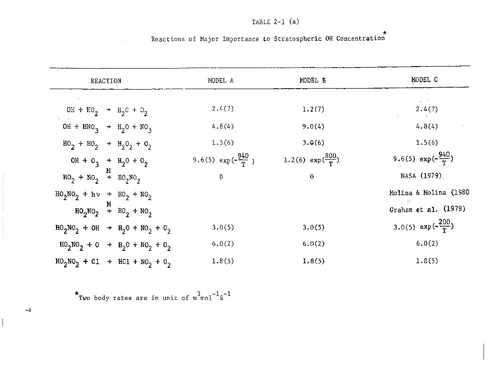
TABLE 2-1 (a)
Reactions of Major Importance to Stratospheric OH Concentratioz
REACTION MODEL A MODEL B MODEL C
OH + HO2 -f H20 -t O2 2.4(7)
OH + HN03 -t H20 tN03 4.8(4)
HO2 + HO2 + H202 t 02 1.5(6)
OH + O3 + H20 t 02 9.6(5) exp(-'+ ) M
HO2 + NO2 -t HO2NO2
H02N02 t hv -t HO2 t NO2 M
HOzNOZ + HO2 + NO2
H02N02 + OH -t Hz0 t NO2 + O2
HOgNO t 0 + Hz0 t NO2 t 02
H02N02 + Cl + HCl t NO2 t 02
0
3.0(5)
6.0(2)
1.8(5)
1.2(7) 2.4(7)
9.0(4) 4.i3(4)
3.9(6) 1.5(6)
1.2(6) exp(F) 9.6(5) exp(- 940 T-)
0 NASA (1979)
Molina & Molina (1980
Graham et al. (1978)
3.0(5)
6.0(2)
3.0(5) w(-2F) 6.0(2)
1.8(5) 1.8(5)
* Two body rates are in unit of m3mol -lS-1
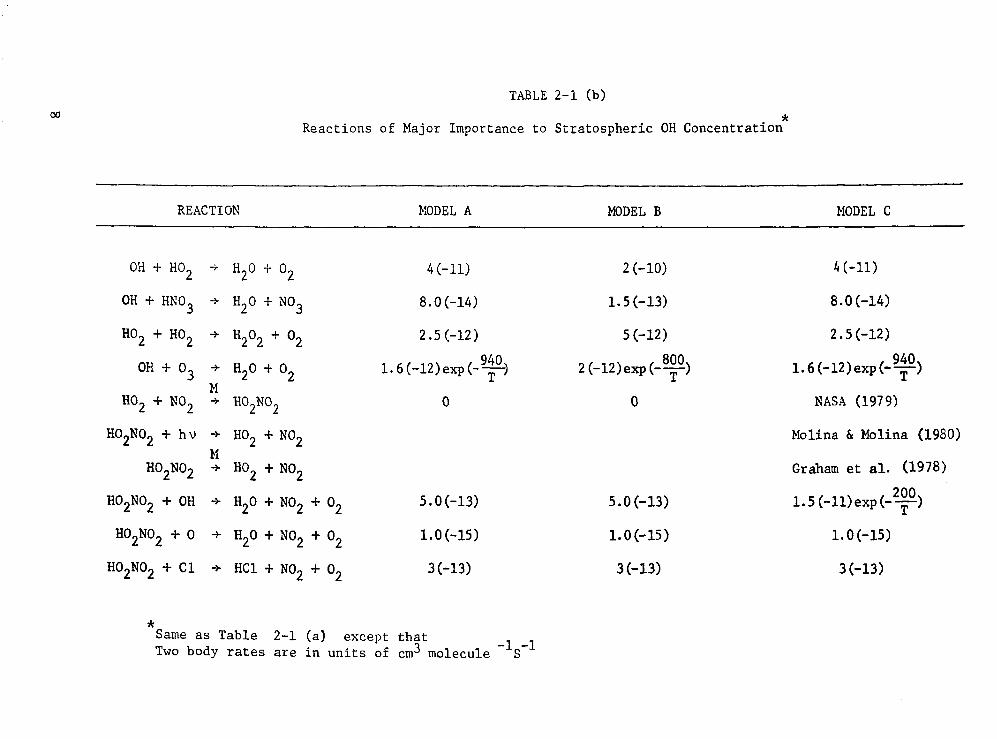
M TABLE 2-l (b)
Reactions of Major Importance to Stratospheric OH Concentration*
REACTION MODEL A MODEL B MODEL C
OH t HO2 + HO+0 2 2 4 (-11)
OH t HN03 + H20 tN03 8.0(-14)
HO2 t HO2 + H202 + O2 2.5(-12)
OH t 03 + H20 t0 940 2 1.6(-12)exp(-T
M HO2 + NO2 -f H02N02
H02N02 + hv + HO2 t NO2 M
H02N02 + HO2 tN02
H02N02 t OH + H20 t NO2 t O2
H02N02 + 0 + H20 t NO2 t O2
H02N02 + Cl + HCl t NO2 t O2
0
5.0(-13)
l.O(-15)
3(-13)
2 (-10) 4 (-11)
1.5(-13) 8.0(-14)
5(-12) 2.5(-12)
2 (-12)exp(-8+) 1.6(-12)exp(-'T)
0
5.0(-13)
l.O(-15)
3(-13)
NASA (1979)
Molina f Molina (1980)
Graham et al. (1978)
1.5(-ll)exp(-2+)
l.O(-15)
3(-13)
* Same as Table 2-l (a) except that Two body rates are in units of cm3 molecule -lS-1
recent cross-section data for H02N02 reported by Molina and
Molinda (1980) are valid and if k12 is faster than 1.2~10~
m3 mol'l s-l (2~10-1~ cm3 s-l).
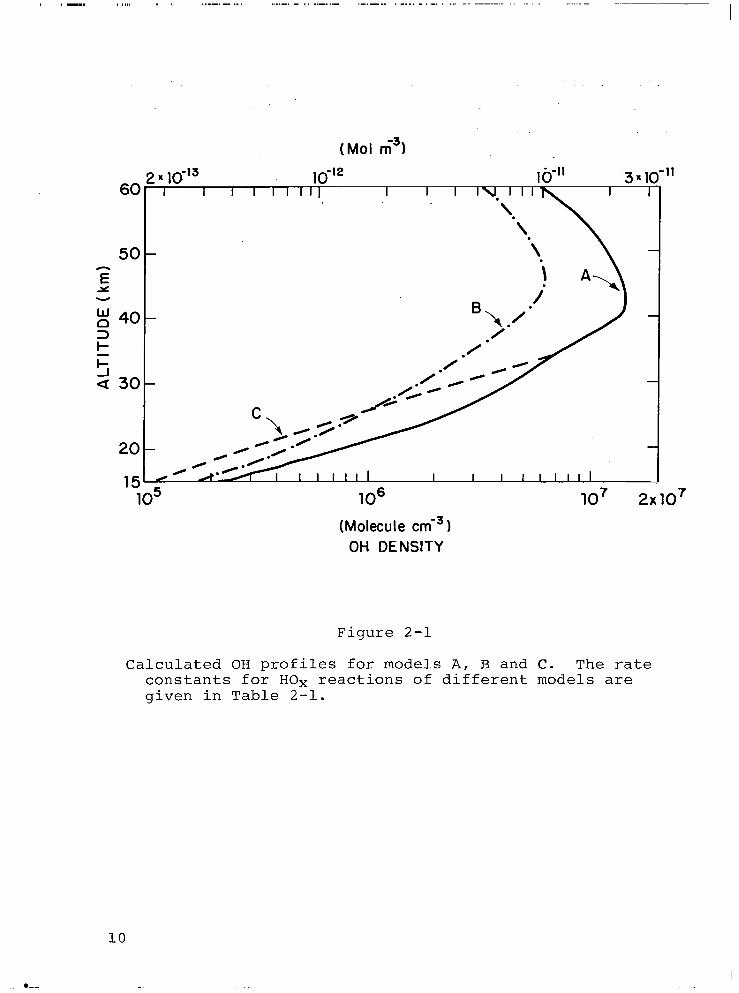
Figure (2-l) shows the calculated OH profiles for
models A, B and C. Note that the OH concentration in model
B is about a factor of two smaller than that in model A
above ~30 km, while the OH concentration is model C is
about a factor of two to three smaller than that in model
A below ~30 km. It should be noted that current measure-
ments of OH are restricted above 30 km. Concentrations of
OH below 30 km can only be indirectly inferred from other
observed quantities such as the gradients of Cl0 and the
HN03:N02 and HF:HCl ratios.
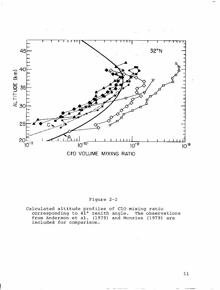
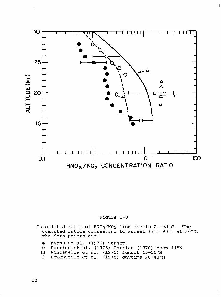
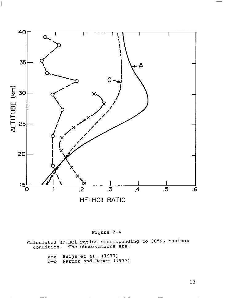
Figures (2-2) through (2-4) show the calculated pro-
files of ClO, HN03/N02 and HF/HCl, along with available
observations. We may note that results from Model C pro-
vide significantly better agreement with observations
(Figures 2-2, 2-3, 2-4) than model A.
2.3 Perturbation Studies
For each model of HO, chemistry, we consider two
different NO, injection altitudes, one at 15-16 km and the
other at 20-21 km. Table 2-2 summarizes the calculated
column perturbations which may result from the operation
of 1000 aircraft, flying 7 hours per day at two different
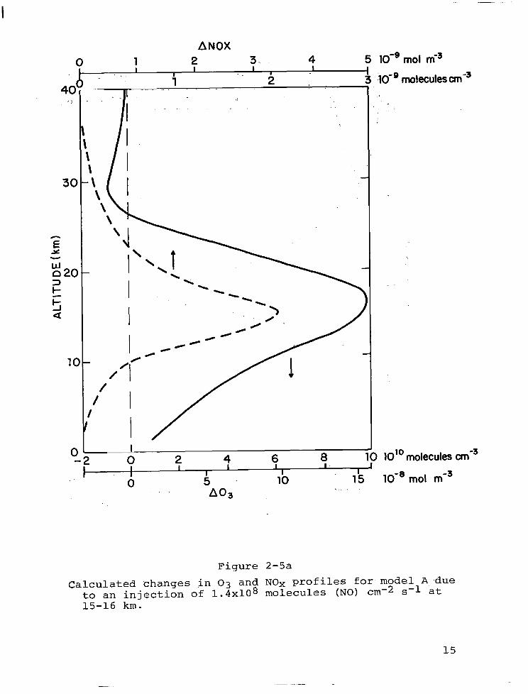
cruise altitudes. Figures (2-5a,b) and (2-6a,b) present
the calculated local ozone and NO, perturbations associated
with supersonic aircraft operation.
Model A predicts increases of about 1.6 and 4 percent
in column ozone for the 15 and 20 km injections respective-
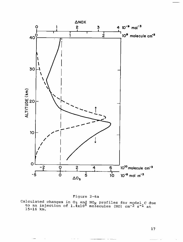
ly* On the other hand, model C predicts a small increase
in column ozone for the low altitude injection but a fairly
large decrease of about 6 percent for the high altitude
injection case. The calculated column ozone perturbations
I I mm-,.. 111.1 . I , . .._. _.. ,,. . . .._. ._ _.-. ..- .._. .-.. __ . . . . _ .-. . . - --.----..- . -. I
60
“\ - B>./ A I .
(Molecule cmw3 I OH DENSITY
Figure 2-l
Calculated OH profiles for models A, B and C. The rate constants for HOx reactions of different models are given in Table 2-l.
10
.- .-
CtO VOLUME MIXING RATIO
Figure 2-2
Calculated altitude profiles of Cl0 mixing ratio corresponding to 41° zenith angle. The observations from Anderson et al. (1979) and Menzies (1979) are included for comparison.
11
3OL I I I I lyrl I I I I Ill1 \
0.1 I I I IIIII I I I I Ill1 I I I lllll
1 10 . 100 HNQ /NO2 CONCENTRATION RATIO
Figure 2-3
Calculated ratio of HN03/N02 from models A and C. The computed ratios correspond to sunset (x = 90°) at 30°N. The data points are:
0 Evans et al. (1976) sunset 0 Harries et al. (1976) Harries (1978) noon 44'N
D Fontanella et al. (1975) sunset 45-5O"N A Lowenstein et al. (1978) daytime 20-40°N
12
20
150’ .1 .2 .3 .4 .5 .6
HF : HCt RATIO
Figure 2-4
Calculated HF:HCl ratios corresponding to 30°N, equinox condition. The observations are:
x-x Buijs et al. (1977) o-o Farmer and Raper (1977)
13
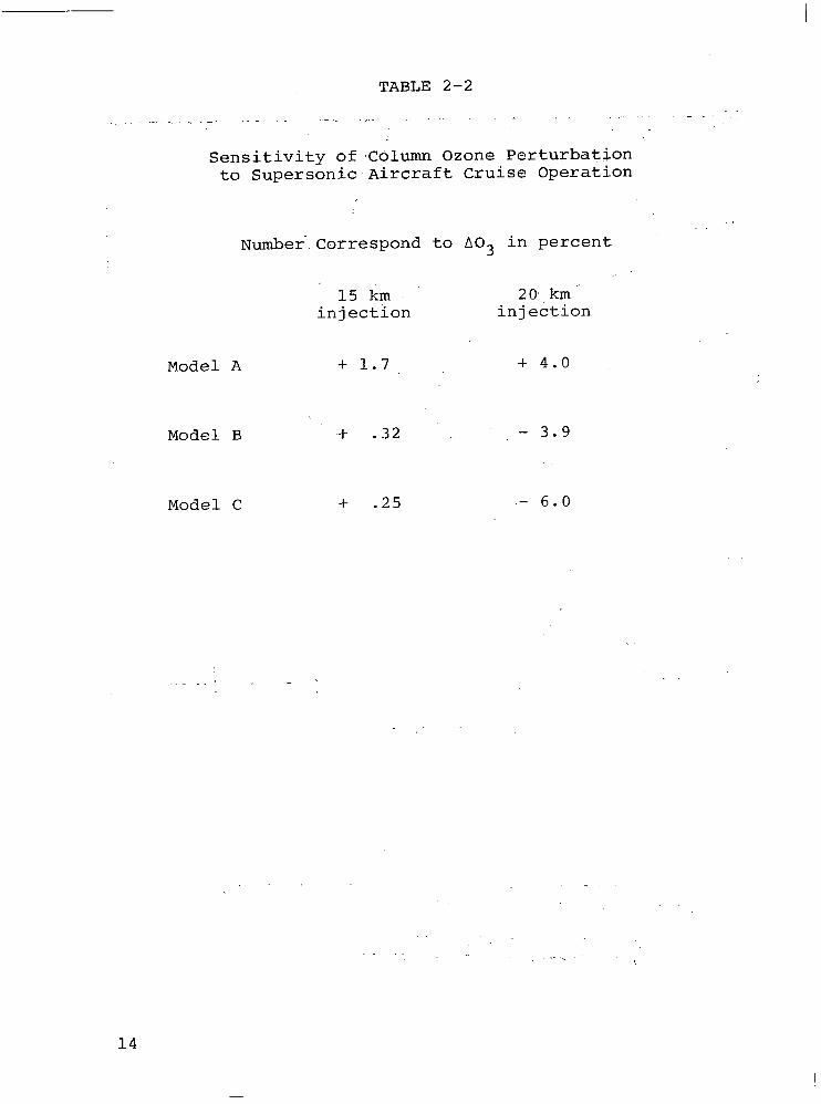
TABLE 2-2
_ ,.. - - _ ., .- ._
Sensitivity of,Column Ozone Perturbation to Supersonic Aircraft Cruise Operation
Number:Correspond to A03 in percent
15 km 20,. km .. injection injection
Model A -t 1.7 + 4.0
Model B
Model C
+ .32 - 3.9
+ .25 - 6.0
_.._
14
\ \ \ I
P Y w 020 z
5 a
1c
,iO-’ molecules cme3
)-
1 I
O- - -2 0 2 4 6 0 lc)
I I I I 0 5 10 15
A03 ,_
ANOX 1 2 3- 4 5 lo-’ mol me3
10” molecules cmw3
10-e mol md3
Figure 2-5a
Calculated 'changes in 03 and NOx profiles for model A.due to an injection of 1.4~108 molecules (NO) cm-2 s-1 at 15-16 km-
15
0
4oy
ANOX 5 10 15 10” mol ms3 I I I I I I
2 4 6 8 10 10’ molecules cmw3
5 a
10
o- -2
1 0 2 4 6 8 10’Omolecules cnf3 I I I I I I I 1
0 5 10 lOwe mol mB3
A03
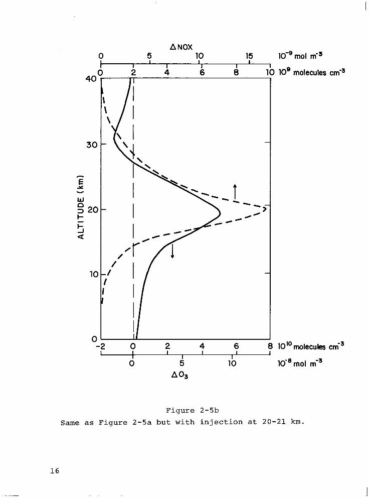
Figure 2-5b
Same as Figure 2-5a but with injection at 20-21 km.
16
ANOX
I- / I /I
/ I / ti
/ I 1 I/
I- I I -2 0 2 4 6
I I -5 0’
I I A03 5 10
lo-’ moly3
10’ molecu
10” molecule crnm3
lo’* mol ms3
Figure 2-6a Calculated changes in 03 and NO x profiles for model C due
to an injection of 1.4~10~ molecules (NO) cmB2 s-1 at 15-16 km.
17
5 “( 10 - -;15 q lo-‘- mol mm3 I I I _ : I I I I
2 .., 4’ ‘- ‘6’ 0‘ ., 10 10’molecules cmS3
\ I \ \
I \
\ /-
0 .-6 -4 -2. 0 2 4
-10 -5 0 5 A03
10” molecules cmS3
lo-* mol mw3
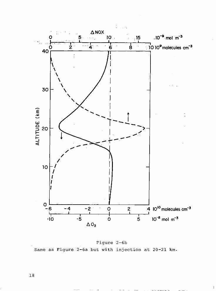
Figure 2-6b
Same as Figure 2-6a but with injection at 20-21 km.
18
.-
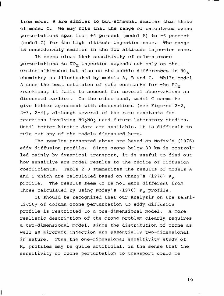
from model B are similar to but-somewhat smaller than those
of model C. We may note that the range of calculated ozone
perturbations span from +4 percent (model A) to -6 percent
(model C) for the high altitude injection case. The range
is considerably smaller in the low altitude injection case.
It seems clear that sensitivity of column ozone
perturbations to NO, injection depends not.only on the- (
cruise altitudes but also on the subtle differences in HOjr
chemistry as illustrated by models A, B and C. While model
A uses the best estimates of rate constants for the HO,
reactions, it fails to account for several observations as
discussed earlier. On the other hand, model C seems to
give better agreement with observations (see Figures 2-2,
2-3, 2-4), although several of the rate constants for
reactions involving H02N02 need future laboratory studies.
Until better kinetic data are available, it is difficult to
rule out any of the models discussed here.
The results presented above are based on Wofsy's (1976)
eddy diffusion profile. Since ozone below 30 km is control-
led mainly by dynamical transport, it is useful to find out
how sensitive are model results to the choice of diffusion
coefficients. Table 2-3 summarizes the results of models 'A
and C which are calculated based on Chang's (1976) Kz
profile. The results seem to be not much different from
those calculated by using Wofsy's (1976) Kz profile.
It should be recognized that our analysis on the sensi-
tivity of column ozone perturbation to eddy diffusion
profile is restricted to a one-dimensional model. A more
realistic description of the ozone problem clearly requires
a two-dimensional model, since the distribution of ozone as
well as aircraft injection are essentially two-dimensional
in nature. Thus the one-dimensional sensitivity study of
K, profiles may be quite artificial, in the sense that the
sensitivity of ozone perturbation to transport could be
19
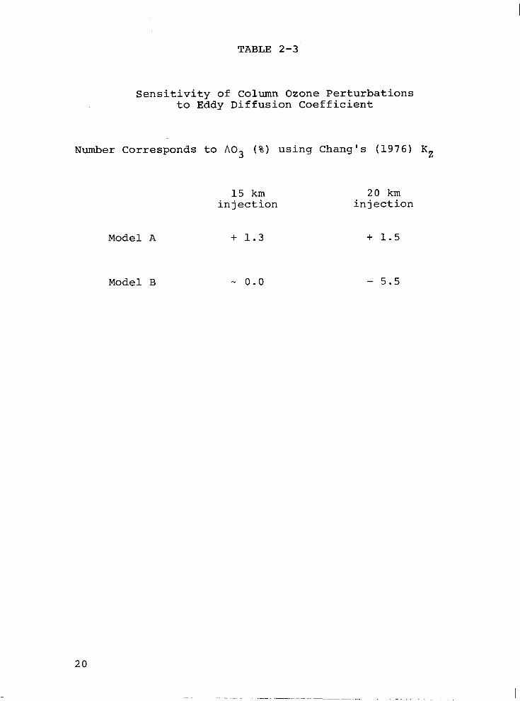
TABLE 2-3
Sensitivity of Column Ozone Perturbations to Eddy Diffusion Coefficient
Number Corresponds to A03 (%) using Chang's (1976) KZ
15 km injection
20 km injection
Model A + 1.3 + 1.5
Model B - 0.0 - 5.5
20
.
quite different in a 2-D model in which both horizontal
and vertical transports are considered.
2.4 Concluding Remarks
We have performed a series of model calculations to
study the sensitivity of column ozone perturbations to the
injection of NO, associated with the operation of super-
sonic aircraft. Because of the coupling nature of hydrogen,
nitrogen and chlorine chemistry, addition of NO, could
either increase or decrease local stratospheric 08. A
model with high background OH concentrations (e.g., model A)
tends to predict an increase in column ozone for low and
high altitude NO, injections. On the other hand, a model
with lower stratospheric OH (e.g., models B and C) tends to
predict a small increase (~1%) in column ozone for the low
altitude injection case but a fairly significant reduction
in column ozone for the high altitude injection case. More
reliable kinetic data are clearly needed to narrow the
uncertainties discussed here. For instance, the rate
constant for the reaction of OH with H02N02 needs to be
measured on a high priority basis. Accurate determination
of this rate constant could either rule out or substantiate
model C.
Changes in local ozone and NO, concentrations in the
stratosphere may also affect the radiation budget. Recent
calculations by Wang and Sze (1980) indicated that a
doubling in NO, may perturb the stratospheric temperatures
and surface temperatures by as much as +1 K and +.15 K
respectively, mainly through redistribution of stratospher-
ic ozone (Wang and Sze, 1980). While changes in stratos-
pheric temperature by 1 K are unlikely to be important in
stratospheric chemistry, changes in surface temperature by
. 15 K are considered to be quite significant when compared
with surface temperature changes caused by other atmospheric trace gases (Wang et al., 1976).
21
3. TWO-DIMENSIONAL ZONAL-MEAN MODELING
3.1 Background
One of the tasks in atmospheric modeling is to attempt
to simulate the behavior of a trace gas in the atmosphere.
The local concentration of a trace gas is governed by the
three-dimensional continuity equation
a (= + yV)f = Q/P (3.1-l)
where f(t,x) is the mixing ratio, v(t,x) the velocity wind
fields describing the general circulation, p(t,x) the air
number density and Q(t,x) is the local net production or
loss (by chemical and/or physical transformation) of the
trace gas. Equation (3.1-l) gives the time rate of change
of f in the Eulerian description of fluid motion. The
quantities f, vI p and Q are to be considered as Eulerian
field quantities as functions of time and spatial location
with coordinates x.
In order to solve equation (3.1-l) for the specie
concentration, one must be able to provide values of v and
temperature T (T is necessary for calculation of reaction
rates) as functions of space and time either by parameter-
ization or by solving the system of dynamic equations. The
atmospheric circulation is governed by the coupled system
of dynamic and thermodynamic equations (cf. Lorentz, 1967)
momentum equation
dv -= dt -2Gxy - -& vp - V@ (3.1-2)
thermodynamic equation
de -= dt J
22
(3.1-3)
continuity equation
dp _ -- dt -pv "y (3.1-4)
equation of state: ideal gas law
= P. PRT (3.1-5)
d where dt = .V is the total time derivative.
The above are to be considered as equations'for the
Eulerian field variables y, p, p and 8. The newly intro-
duced symbols have the following meaning:
R =
M=
P= a =
8 =
J=
R=
T=
angular velocity of Earth
average mass of an air molecule
pressure
the geopotential gz where g is acceleration due
to gravity, z is geometrical altitude
potential temperature related to temperature
T by 8 = T(p)K with K = R/Cp; R the gas constant
and C P
the specific heat at constant pressure
the diabatic influence with C~J~ the heating rate
per unit mass
the gas constant
temperature
Note that we have left out frictional forces in the momen-
tum equation (3.1-2) under the assumption that they are
unimportant for large scale motion.
The system of equations (3.1-2) to (3.1-5) is coupled
to the specie equation through the J term which depends on
distribution of gases such as 03, C02, N20 and CH4 in the
atmosphere. Thus, in principle, equations (3.1-l) through
23
(3.1-5) must be solved simultaneously as a system. In practice, the system of equations presents a
formidable numerical problem and put enormous demand on
both computer core memory and computation time. This is
particularly true if one is interested in a realistic
chemical scheme in order to simulate the distribution of
the various species in the atmosphere. Besides, the set of
exact equations also simulates phenomena of little interest
for large scale motions. The following physical assump-
tions are usually adopted:
A)
B)
C)
Replacement of the vertical momentum equation by
the hydrostatic equilibrium condition, i.e., the
pressure gradient force is balanced by geopotential
term)
ap _ -- az -M P g (3.1-6)
It is observed that motions due to deviation away
from hydrostatic equilibrium are restricted to
oscillations about the equilibrium state with
time scales of order hour. The adoption of
equation (3.1-6) effectively filters out vertically
travelling sound waves.
Discard terms containing the vertical velocities
in the remaining two components of the momentum
equation. This approximation appears to be justi-
fied because of the fact that the vertical compon-
ent of the velocity is about two orders of magni-
tude smaller than the horizontal components.
Replace r in the resulting equation by a where r
is the distance from the Earth's center; a is the
radius of the Earth.
The above assumptions lead to a system of equations
usually referred to as the primitive equations. Next, it
24
would be desirable to write the momentum equation in scaler
form. For this purpose, it is convenient to introduce a
coordinate system where the pressure p is used as the ver-
tical coordinates in conjunction with X the longitude and
@ the latitude. In this coordinate system, the components
of the velocity vectors are
u = dX a cos$ dt
w = dp dt
The continuity equation takes the form
1 *+ 1 a( aw a CO.+ ax a COS@ a$ v cosf$) + ap = 0 (3.1-7)
This is sometimes written in the form
v-v = 0 (3.1-8)
However, equation (3.1-8) holds only in pressure coordin-
ates. Since equation (3.1-7) is derived using only the
hydrostatic equation, it is more general than the incom-
pressible fluid assumption. Finally, from equation
(3.1-7), one can derive (cf. Lorentz, 1967)
ds -= 22. dt at
(3.1-9)
for any scaler s.
In this coordinate system, the primitive equations are
(cf. Lorentz, 1967; Holton, 1975)
-
25
af + 1 at -2 MU) + a ios$ ?$ a cos$ 3A (fv co@) + $ (fw) = !j!
(3.1-10)
?E: 1 at -2 h2) + a iosg 6 a cos$ aA (uv cosql) + g (uw) (3.1-11)
_ uv tan@ a - 2Rv sin@ - g az - = 0 a cos$ 8A
g+ 1 -2 (vu) + a kos$ $ (v2cosc$) a a COS+ ax + ap (VW)
+ u2 tan@ g az a + 2Ru sin@ - a w = 0
(3.1-12)
1 a COSC$ &- (eu) + a ioso i& (ev ~0s~) + $ (ew) = J
(3.1-13)
1 25. 1 a COS$ ah 4 aw
a COS$ a$ v cos@) + - = 0 ap (3.1-14)
P = P RT (3.1-15)
az 1 gap = -pM (3.1-16)
In the above equations, the terms uv tan' and a
u2 tan@ are a
curvature terms arising from the non-Euclidean nature of
the coordinate frames. 1
The geopotential term &- g and a a+
.?a a has been written out explicitly with 0 = gz. COS+ ax
In this arrangement, equations (3.1-10) through (3.1-13) are prognostic equations for f, u, v and 8
respectively, while equations (3.1-14) and (3.1-15) can be
26
considered as diagnostic equations for w and p. Since p is
being used as an independent variable, equation (3.1-16)
serves the purpose of transforming between geometrical
altitude and the pressure coordinate.
We will now discuss ways of reducing the system of
primitive equations to 2 dimensions for numerical modeling.
Taking any of the dependent Eulerian variables in the
primitive equations, e.g., f, by averaging over one of the
spatial coordinates, one obtains F (t,y) where y is the
vector representing the two remaining coordinates.
The corresponding equations governing the averaged
variables can be obtained by applying the averaging opera-
tion to the primitive equations. In atmospheric modeling
studies, one is interested in averaging over the longitud-
inal coordinate to obtain r as a function of time, latitude
and altitude, which can be viewed as the zonal-mean concen-
tration. However, the exact physical interpretation of F
must depend on the averaging process involved.
In all of the 2-D zonal-mean models currently in use
(cf. Hidalgo and Crutzen, 1977; Louis et al., 1974; Whitten
et al., 1977; Borucki et al., 1976; Vupputuri, 1973;
Harwood and Pyle, 1975) the Eulerian-mean
operation is used exclusively. In the context of the
present discussion, the most important feature in a
Eulerian-zonal-mean model is the treatment of tracer
transport. In these models, the flux into or out of a
volume element is comprised of two terms: the flux due to
advection by the zonal-mean velocity and the contribution
due to the so-called "eddy fluxes". Several studies
(Sawyer, 1965; Mahlman, 1975; Matsuno, 1979; Plumb, 1979)
have found the above feature in the Eulerian-mean model to
be undesirable and further work (Andrew and McIntyre, 1978;
Dunkerton, 1978; Matsuno and Nakamura, 1979; Matsuno, 1980;
Mahlman et al., 1980) eventually led to the development of
27
the generalized Lagrangian-mean (GLM) theory. As demon-
strated by Andrew and McIntyre (1978), the flux of a trace
gas in the GLM formulation is given as an advection term by
a GLM velocity. Further studies by Dunkerton (1978) showed
that this GLM velocity could be approximated from consider-
ation of atmospheric heat balance.
It is the purpose of this section to discuss the
possibility of applying the GLM theory to numerical zonal-
mean modeling of atmospheric trace gases. In the next
section, we will begin with a review of the current
Eulerian-mean models in order to put the problem into
proper perspective.
3.2 Eulerian-Mean Model
In the Eulerian-mean model, the averaging process is
performed over Eulerian field quantities by integrating
over one of the coordinates while holding all other coor-
dinates fixed. In the case of the atmospheric models, the
integration over the longitude is done along constant lati-
tude circles, altitudes and time. Thus, given g(tl~,pr~),
(where t is time, C$ the latitude, p the pressure height
coordinates and X the longitude), one obtains
C(t,$,p) = J g(t,Grp,X)dX 1 dX
(3.2-l)
It is convenient to define g', the deviations from the
mean, by
g’ (t,o,p,A) = s (t,$,P) - g (t,@,P,X) (3.2-2)
It follows from equation (3.2.1) that
g’(t,$,p,X) = O (3.2-3)
and
gh=gg+g’h’ (3.2-4)
When the Eulerian-mean operation is applied to
equations (3.1-10) to (3.1-16), using the fact that the
IS-~ operation commutes with the coordinate differential
operators, we have
- 1 -_ 0 a (z v COS@) + $ (f W) = (,) - Ff a COS$ a$ (3.2-5)
a -- - v cos2$) + ap (u WI- 252~ cos@ = -FU
(3.2-6)
- E+ 1
4 -2 --L
v cos@) + -2 (V W) + u tan@ a COS$ a$ ap
a
(3.2-7) g aF + 2 u R sin@ - - - = -Fv a a$
- E+ 1 --
a (e v COS@) + $ (8 w) = r - Fe a COS$ aa (3.2-8)
1 a cos$ +@ =o
ap (3.2-9)
g = RF B (3.2-10)
az --=-R~ 1 gap = MD Mp (3.2-11)
29
where Ff = 1 -2 (f'v' a a CO@ a+
cost)) + ap (W)
FU = 1 -? (v'u' a cos2$ a@
cos2$) + -2 (u'w') ap
Fv = 1 a (,I2 -tan+ U a COS@ a+
cos@) + ap v'w') + a ( a
Fe = 1 2 (0'V a a ~0.34 a+
c0se) + ap (e'w')
are the eddy flux divergence terms. Note that in equation
(3.2-61, we have incorporated the curvature term ( uv tan@ a ) a into the p term. It should be emphasized that the eddy
flux terms are not constrained by the system of equations
and must be specified or parameterized in terms of other
variables.
In zonal-mean models, a further physical assumption is
usually adopted. From scale analysis, it can be shown (cf.
Holton, 1975) that equation (3.2-7) reduces to
g aZ 2R sine< = a z (3.2-12)
to lowest order of a Rossby number expansion. This is the
geostrophic assumption which provides a good approximation
for midlatitude dynamics though some authors (Harwood and
Pyle, 1975) argued that the approximation is reasonable up
to about 5O. The geostrophic assumption filters out occur-
rance of gravity waves and other equatorial waves that
cause the quasi-biennial oscillations in the stratosphere.
Equation (3.2-12) is awkward to use as z is not one of the
dependent variables. One can differentiate the equation
30
with respect to p and use the hydrostatic equation to
obtain the thermal wind relation
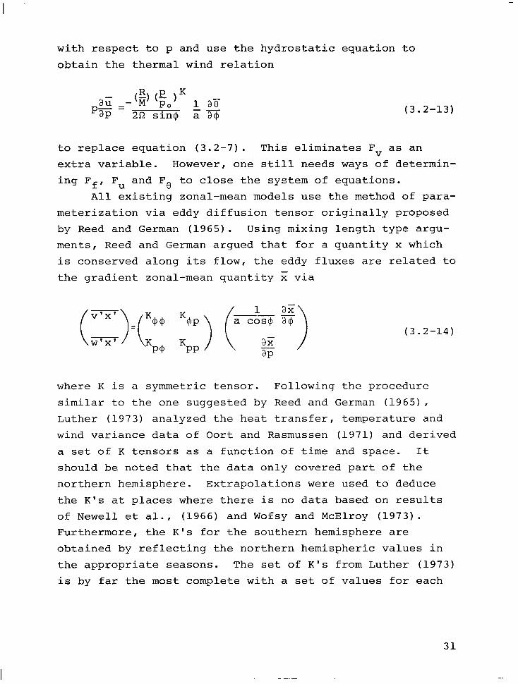
(3.2-13)
to replace equation (3.2-7). This eliminates Fv as an
extra variable. However, one still needs ways of determin-
ing Ff, FU and F6 to close the system of equations.
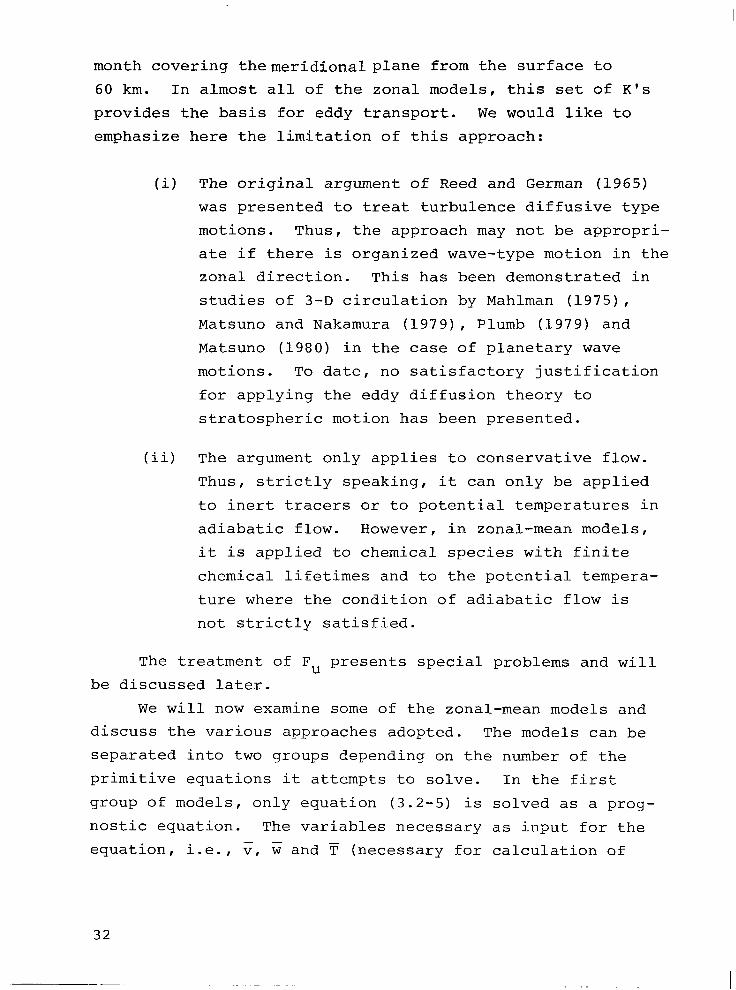
All existing zonal-mean models use the method of para-
meterization via eddy diffusion tensor originally proposed
by Reed and German (1965). Using mixing length type argu-
ments, Reed and German argued that for a quantity x which
is conserved along its flow, the eddy fluxes are related to
the gradient zonal-mean quantity x via
(3.2-14)
where K is a symmetric tensor. Following the procedure
similar to the one suggested by Reed and German (1965),
Luther (1973) analyzed the heat transfer, temperature and
wind variance data of Oort and Rasmussen (1971) and derived
a set of K tensors as a function of time and space. It
should be noted that the data only covered part of the
northern hemisphere. Extrapolations were used to deduce
the K's at places where there is no data based on results
of Newell et al., (1966) and Wofsy and McElroy (1973).
Furthermore, the K's for the southern hemisphere are
obtained by reflecting the northern hemispheric values in
the appropriate seasons. The set of K's from Luther (1973)
is by far the most complete with a set of values for each
31
month covering themeridional plane from the surface to
60 km. In almost all of the zonal models, this set of K's
provides the basis for eddy transport. We would like to
emphasize here the limitation of this approach:
(i) The original argument of Reed and German (1965)
was presented to treat turbulence diffusive type
motions. Thus, the approach may not be appropri-
ate if there is organized wave-type motion in the
zonal direction. This has been demonstrated in
studies of 3-D circulation by Mahlman (1975),
Matsuno and Nakamura (1979), Plumb (1979) and
Matsuno (1980) in the case of planetary wave
motions. To date, no satisfactory justification
for applying the eddy diffusion theory to
stratospheric motion has been presented.
(ii) The argument only applies to conservative flow.
Thus, strictly speaking, it can only be applied
to inert tracers or to potential temperatures in
adiabatic flow. However, in zonal-mean models,
it is applied to chemical species with finite
chemical lifetimes and to the potential tempera-
ture where the condition of adiabatic flow is
not strictly satisfied.
The treatment of FU presents special problems and will
be discussed later.
We will now examine some of the zonal-mean models and
discuss the various approaches adopted. The models can be
separated into two groups depending on the number of the
primitive equations it attempts to solve. In the first
group of models, only equation (3.2-5) is solved as a prog-
nostic equation. The variables necessary as input for the
equation, i.e., V, w and T (necessary for calculation of
32
--- -
-
reaction rate constants) are parameterized. In addition,
a chemical scheme has to be set up to calculate the produc-
tion and loss term Q. The models of Hidalgo and Crutzen
(1977) I Louis et al., (1974), Widhopf (1975), the NASA Ames
Model(Whitten et al., 1977; Borucki et al., 1976) and the
Meteorology Office Model (Hinds, 1979) fall into this
category.
Strictly speaking, the v, w and F specified must satis-
fy equations (3.2-7) through (3.2-9). The circulations
used in most of these zonal models are based on the work of
Louis et al., (1974) who computed the circulation patterns
for each season by solving the continuity equation (3.2-9)
and energy equation (3.2-8) using the compiled observations
of localmeridionaltemperature distribution and heat trans-
fer rates. However, interpolations and adjustments are
usually made subsequently by the individual authors. In
those cases, w is obtained by solving equation (3.2-9) once
v has been chosen in order to assure mass conservation. In
models that use pressure coordinates, the hydrostatic
equilibrium assumption is implicit in equation (3.2-9). In
some models, e.g., the NASA Ames Model, geometrical alti-
tude is used instead. In this particular model, the zonal-
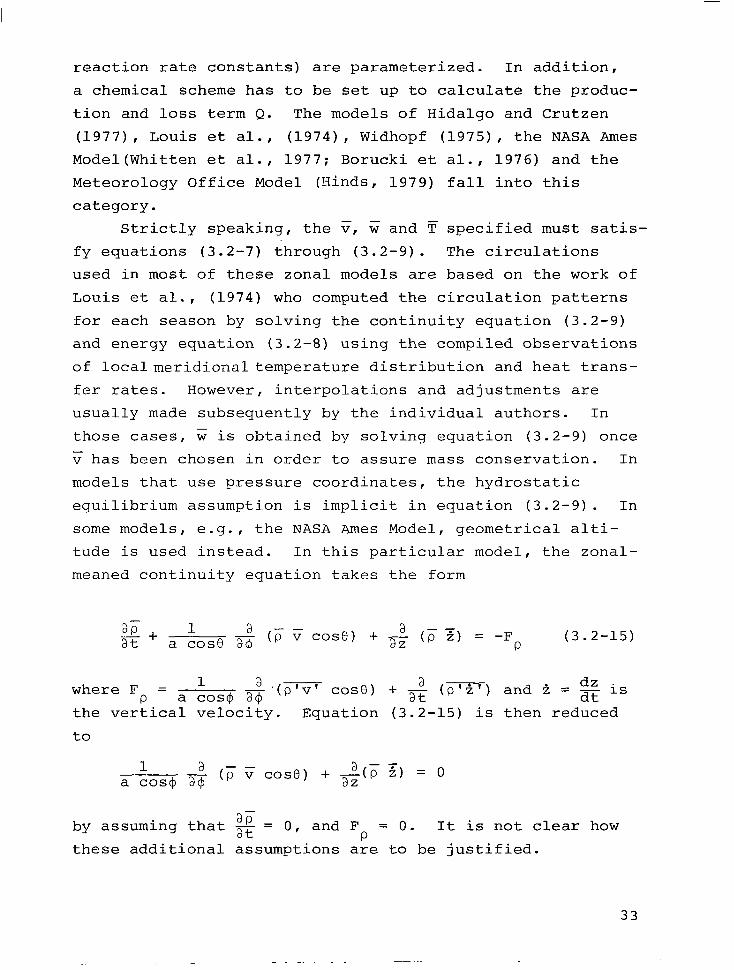
meaned continuity equation takes the form
aF at+
1 --ii (p c case) + 2 (p H) = -Fp a cosf3 a$ (3.2-15)
where F = 1 P
a '(P'V' dz a COS$ a$
case) + & (p'i') and i = dt is
the vertical velocity. Equation (3.2-15) is then reduced
to
1 -2 (p v cos0) + a COS$ a@ &P 8, = 0
- by assuming that g = 0, andF =O. It is not clear how
P these additional assumptions are to be justified.
33
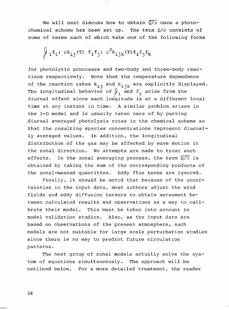
We will next discuss how to obtain Q/p once a photo-
chemical scheme has been set up. The term Q/P consists of
sums of terms each of which take one of the following forms
ifii Pkij (T) fifj; p2kijk(T)fifjfk
for photolytic processes and two-body and three-body reac-
tions respectively. Note that the temperature dependence
of the reaction rates k.. and k.. 17
!
Ilk are explicitly displayed.
The longitudinal behavior of /I i and f i arise from the
diurnal effect since each longitude is at a different local
time at any instant in time. A similar problem arises in
the 1-D model and is usually taken care of by putting
diurnal averaged photolysis rates in the chemical scheme so
that the resulting species concentrations represent diurnal-
ly averaged values. In addition, the longitudinal
distribution of the gas may be affected by wave motion in
the zonal direction. No attempts are made to treat such
effects. In the zonal averaging process, the term Q/p is
obtained by taking the sum of the corresponding products of
the zonal-meaned quantities. Eddy flux terms are ignored.
Finally, it should be noted that because of the uncer-
tainties in the input data, most authors adjust the wind
fields and eddy diffusion tensors to obtain agreement be-
tween calculated results and observations as a way to cali-
brate their model. This must be taken into account in
model validation studies. Also, as the input data are
based on observations of the present atmosphere, such
models are not suitable for large scale perturbation studies
since there is no way to predict future circulation
patterns.
The next group of zonal models actually solve the sys-
tem of equations simultaneously. The approach will be
outlined below. For a more detailed treatment, the reader
34
is referred to the work of Harwood and Pyle (1975) and
Vupputuri (1973).
Equations (3.2-6) and (3.2-8) can be written as
aii -= at A
aTJ -= at B
(3.2-16)
(3.2-17)
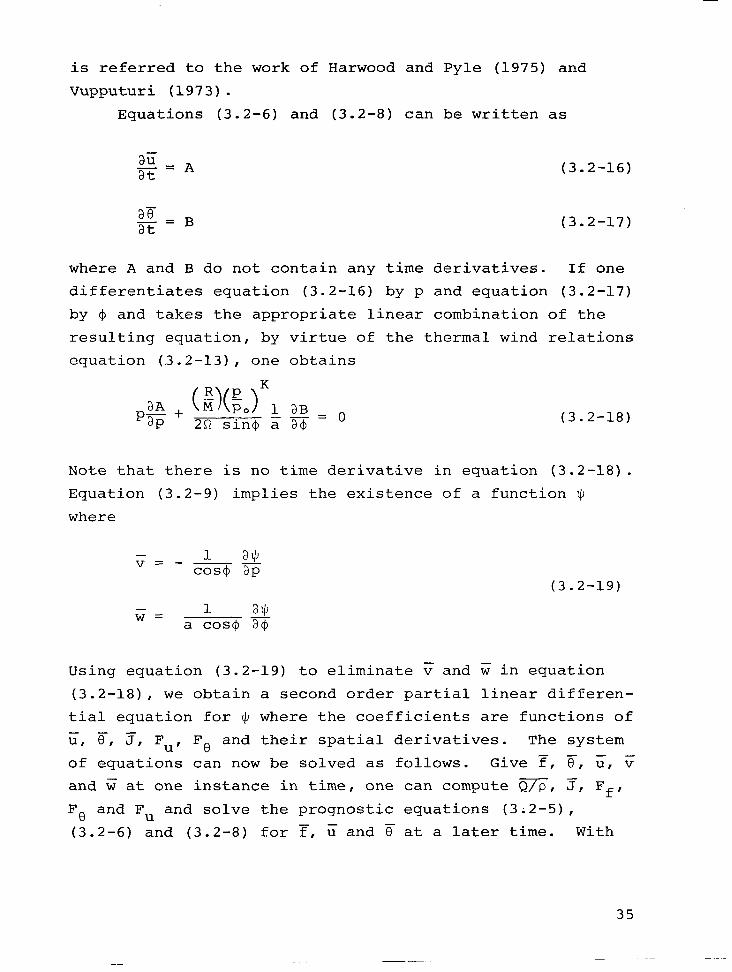
where A and B do not contain any time derivatives. If one
differentiates equation (3.2-16) by p and equation (3.2-17)
by 4 and takes the appropriate linear combination of the
resulting equation, by virtue of the thermal wind relations
equation (.3.2-13), one obtains
pa$ + (SJKl aB --= 2R sin@ a a$ O
(3.2-18)
Note that there is no time derivative in equation (3.2-18).
Equation (3.2-9) implies the existence of a function $
where
(3.2-19)
W= 1 w a cos@ a
Using equation (3.2-19) to eliminate v and w in equation
(3.2-18), we obtain a second order partial linear differen-
tial equation for $ where the coefficients are functions of
u, ?tj-, r, F U’ Ft3 and their spatial derivatives. The system
of equations can now be solved as follows. Give F, e, u, v
and w at one instance in time, one can compute QT, 3, F f'
Fe and FU and solve the prognostic equations (3.2-5),
(3.2-6) and (3.2-8) for F, u and e at a later time. With
35
these new values, one solves equation (3.2-18) for $ with
appropriate boundary conditions and generate new c and w
via equation (3.2-19). The terms QIP are to be calculated
as discussed before. The treatment of 5 is similar in that
the term is obtained by using zonal-meaned values in the
expression while ignoring eddy flux terms. Ff and FO are
to be parameterized by eddy diffusion tensors. The treat-
ment of FU is more difficult because the u momentum is
definitely not conserved in the flow. Attempts to para-
meterize FU in terms of potential vorticity and potential
temperature has little success (Green, 1970; Wiin-Neilsen
and Sela, 1971). Vupputuri (1979) employed an ad hoc para-
meterization while Harwood and Pyle (1975) deduced the
momentum fluxes from Nimbus V SCR data. Until a more
satisfactory theoretical approach is available, the satel-
lite data approach seems to be preferrable at this stage.
Thus, even in the case when one actually computes the
circulation and temperature, one still has to depend on
observations to parameterize the eddy flux terms. It is
also noted in the calculation of Harwood and Pyle (1977)
that the fluxes due to the mean circulation are often in
opposite direction to eddy fluxes. Thus, the net transport
is the difference between the two terms. This suggests the
act of splitting the transport term into the advection and
eddy fluxes components may not be appropriate. It is the
desire to get away from eddy flux formulation that led to
the development of the generalized Lagrangian-mean zonal
models.
3.3 Generalized Lagrangian-Mean (GLM) Zonal Models
An alternative to the Eulerian approach of fluid motion
is the classical Lagrangian approach. In such an approach,
one is interested in how a quantity changes as one follows
the motion of the fluid. More specifically, the property
36
g is given by the function g(t,s) where s(t,i) is the posi-
tion vector of a fluid particle labelled by g. This method
has been used to study the general circulation in three
dimensions in several studies (cf. Riehl and Fultz, 1957;
Krishnamurti, 1961; Danielson, 1968; Mahlman, 1969, 1973).
Further developments in an attempt to apply the Lagrangian
type dynamics treatment to zonal-mean quantities led to the
development of the Generalized Lagrangian-Mean (GLM) theory
(Andrew and McIntyre, 1978; Kida, 1977; Dunkerton, 1978;
Matsuno and Nakamura, 1979; Matsuno, 1980).
It should be noted that the GLM zonal approach is
actually a combination of Eulerian-Lagrangian descriptions
of fluid motion. One actually starts with the Eulerian
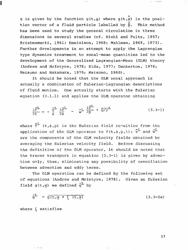
equation (3.1.1) and applies the GLM operator obtaining
aFL vL afL - afL -=-- - - at a a@
WLap + QXL (3.3-l)
-L where f (t,+,p) is the Eulerian field relultincr from the
application of the GLM operator to f(t,$,p,X); vL and wL
are the components of the GLM velocity fields obtained by
averaging the Eulerian velocity field. Before discussing
the definition of the GLM operator, it should be noted that
the tracer transport in equation (3.3-l) is given by advec-
tion only, thus, eliminating any possibility of cancellation
between advection and eddy terms.
The GLM operation can be defined by the following set
of equations (Andrew and McIntyre, 1978). Given an Eulerian
field g(t,x) we defined sL by
-L g = g&x + 5 (L$ (3.3-2a)
where 5 satisfies
37
or
and
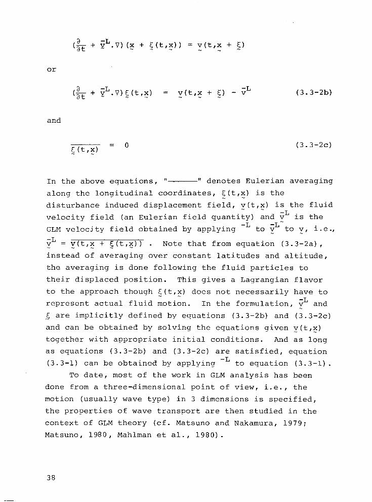
a -L (at + v .v> (5 + gt,+ = v(t,x + 3)
a -L (at + p Jog (-Q) = y(t+ + 5) - vL
$(bx) = O
(3.3-2b)
(3.3-2~)
In the above equations, U W denotes Eulerian averaging
along the longitudinal coordinates, <(t,x) is the
disturbance induced displacement field, v(t,x) is the fluid -L
velocity field (an Eulerian field quantity) and v is the
GLM velocity field obtained by applying -L to GL to v, i.e.,
FL = y(t,x + gt,g 1 - Note that from equation (3.3-2a),
instead of averaging over constant latitudes and altitude,
the averaging is done following the fluid particles to
their displaced position. This gives a Lagrangian flavor
to the approach though <(t,x) does not necessarily have to
represent actual fluid motion. -L In the formulation, v and
5 are implicitly defined by equations (3.3-2b) and (3.3-2~)
and can be obtained by solving the equations given v(t,x)
together with appropriate initial conditions. And as long
as equations (3.3-2b) and (3.3-2~) are satisfied, equation
(3.3-l) can be obtained by applying -L to equation (3.3-l).
To date, most of the work in GLM analysis has been
done from a three-dimensional point of view, i.e., the
motion (usually wave type) in 3 dimensions is specified,
the properties of wave transport are then studied in the
context of GLM theory (cf. Matsuno and Nakamura, 1979;
Matsuno, 1980, Mahlman et al., 1980).
38
In a zonal model, one-;ould like to integrate equation
(3.3-l) in time to obtain f as a function of time. Thus, -L it is necessary to obtain v -L and w without a priori
knowing the 3-dimensional general circulation. Secondly,
one has to be more specific in the definition of 5 so that
a physicalLinterpretation can be given to the GLM operation
and that f can be compared to observations. We will
discuss these problems in what follows.
(a) Interpretation of 5 and -L
In the formulation of Andrew and McIntyre (1978), the
definition of 5 is purposely left vague in order that the
formalism can be applied to any averaging operations. The
quantity c(t,x) is loosely referred to as the disturbance
induced displacement vector. One can imagine the situation
in which a parcel of air molecules is initially at rest on
a latitudinal circle at constant altitude [G]. (Note that
[G] stands for a latitude circle at constant altitude). At t = t,, the molecules start executing motions given by
$ct,gl, i.e., the coordinate of the particle initially
located at G is given at time t by i + <(t,G). Then
according to equation (3.3-2a), instead of averaging over
the particles that happen to be located at G at time t, the
averaging is done following the fluid particles as they
travel along the trajectory <(t,G). If <(t,G) satisfies
equations (3.3-253) and (3.3-2c), then the averaging pro- -L ceeding qualifies as GLM operation, and v can be inter-
preted as the motion associated with the center of mass of
the air parcel originally located at i. This interpreta-
tion has been presented by Andrew and McIntyre (1978) using
their mechanical analog and is essentially the same as
interpretations presented by other authors (Dunkerton,
1978; Mahlman et al., 1980).
39
The above interpretation of vL is contingent upon the
fact that <(t,G)satisfies equations (3.3-2b) and (3.3-2~).
In general, this will not hold for Lagrangian trajectory of
the fluid. However, since c(t,G) is defined by the current
positions of the particles as well as 5, one can redefine
5 as <(t,xO) so that equations (3.3-2b) and (3.3-2~) are
satisfied (Tung, private communication). The details of
this manipulation will be presented in Appendix E.
Under the initialization process, fL can be inter-
preted as the average mixing ratio of the air molecules
that would have been located at x, in the absence of the
disturbance induced displacement. Similarly, Q/pL is the
average production rate of the same set of molecules and ;L -L and w are the components of the velocity associated
with the center of mass of that air parcel.
Note that a parcel of air has a tendency to spread out
because of diffusion. Thus, the magnitude of <(t,x,) would
get progressively larger. It will then become increasingly
difficult to relate zL to actual observations as the indiv-
idual molecules that enter into the averaging process are
distributed over the entire atmosphere. The same applies -L to the computation of Q/pL in the sense that Q/p at some
particular latitude and height may diff:; significantly
from the corresponding products of the f s at the same
point.
(b) Determination of GL and wL
In order to use equation (3.3-l) as a prognostic
equation, -L one needs the values v -L and w . If the three-
dimensional motion is known, one can conceivably solve -L equation (3.3-2b) and (3.3-2~) for < and v with choice of
initial conditions. However, if one is interested in a
zonal model than can include feedback mechanisms between
chemistry and dynamics, one would have to be able to obtain
40
vL -L and w without a priori knowledge of the motion.
One possible approach is to try to obtain vL -L and w
from the GLM momentum equation. Unfortunately, as demon-
strated in Andrew and McIntyre (1978), the price paid for
the simplification in equation (3.3-l) is that -L no longer
commutes with the coordinate differential operators. For
example, the GLM flow of an incompressible fluid satisfying
V.v = 0 is not non-divergent, i.e. V.cL # 0, in contrast to
the case of Eulerian mean flow. Another result of the non-
commutability of the operator -L and V is that the GLM
momentum equation contains terms involving 5, i.e.
TJpL = OpL + (term involving < and derivative of 5)
These terms are reminiscent of the eddy flux terms in the
Eulerian mean formulation and require parameterization.
Dunkerton (1978) suggested an alternative approach to
the problem from analysis of the thermodynamic equation.
Using a linearized version of GLM theory for steady waves,
Dunkerton showed that under certain conditions
$J = ,,e,
1 a (--L a COS@ a$
v COSQ) aiGL o + - = aP
(3.3-3)
(3.3-4)
where a is the Eulerian mean diabatic heating rate, r,-r
is the lapse rate. The 3-D equation for potential tempera-
ture can be written
a (TF -
+ v.V)T = Q (3.3-5)
where Q is the diabatic heating. Upon GLM averaging one
obtains
41
aTL VL aTL at +a s
+ ;L aTL = EL Bp .- (3.3-6)
Equation (3.3-3) can be derived from equation (3.3-6) if
the following assumptions are made (Dunkerton, 1978)
(i)
(ii)
(iii)
(iv)
aTL at
negligible
CL aTL a v
Q -L 2 a
negligible
so that CL ap zr
Equation (3.3-4) is the continuity equation obtainable from
the GLM equation by discarding terms of O(c2). Using the
heating rate of Murgatroyd and Singleton (1961), Dunkerton -L
solved equations (3.3-3) and (3.3-4) for v -L and w and
obtained results that are capable of explaining the gross
features of tracer transport.
Although the assumption used in deriving equations
(3.3-3) and (3.3-4) may not be valid in the whole atmos-
phere, the result of Dunkerton is beautiful in its concep-
tual simplicity in relating the circulation to diabatic
heat balance. However, the application of the results to
zonal modeling may not be straight forward. The situation
is particularly difficult in dealing with finite amplitude
motions.
3.4 Concluding Remarks
In this section, we have presented a brief review of
the generalized Lagrangian mean description of atmospheric
circulation. Most of the studies done to date in GLM
42
theory have been concerned with applying the technique in
analyzing the transport due to specific wave motions [in 3
dimension] in the atmosphere. In this section we have
taken the view of trying to use equation (3.3-l) as the
prognostic equation in zonal modeling.
The zonal mean tracer equation (3.3-l) is attractive
in that the only transport of tracer is due to advection by
the Lagrangian mean velocity only. From our studies, we
identified several crucial areas that need to be investi-
gated in order that the GLM tracer equation can be profit-
ably applied to zonal modeling. The first of these has to
do with the basic interpretation of equation (3.3-l). As
demonstrated in Section (3.3) and Appendix E, the distur-
bance induced displacement vector can be related to the
actual fluid motion. -L Then f can be interpreted as the
average mixing ratio of the air molecules in an air parcel
originally located at [i] where [;I stands for the coordin-
ates of the set of points on a latitude circle at constant
altitude. Though the idea of keeping track of the identity
of the molecules may be very useful in the analysis of mass
transport, it may introduce complications in modeling of
trace gases. As an air parcel is spread out thinner and
thinner over an ever increasing region of the atmosphere, -L it becomes almost impossible to relate f to the local
observed concentrations. This suggests that one may want
to relax the rigid relation between 5 and the trajectory
introduced in Appendix E and employ different initializa-
tions during the time integration of equation (3.3-l) using
each initialization for only short time intervals.
An ideal zonal model should be able to compute the
circulation given the ambient concentrations of the trace
gas and the state of the atmosphere. Thus, it would be -L nice if there is some way to solve for v -L and w as
functions of zLs and temperature. Such an approach will
require research into the reformulation of the momentum
43
equation. By defining some kind of generalized differen-
tial operators, it may be possible to cast the momentum
equation in a form that has no explicit dependence in 5.
The above areas involve long term developments. On
the more immediate term, one can still explore the merits -L of the GLM model by using v and wL derived from given
three-dimensional motion fields. The initial analysis
could be applied to studies of inert tracers, thereby
avoiding the question about Q/pL. Numerical experiments
dealing with inert tracer release can be done. Such exper-
iments will be more meaningful if the results can be
compared with results from similar experiments using
Eulerian mean models. One can then compare the center of
mass motion obtained from the Eulerian model to see if it
bears any resemblence to vL -L and w .
One could also concentrate on cases with small distur-
bances and make use of the results of Dunkerton (1978) to
generate the wind fields. The heating rate of Murgatroyd
and Singleton (1961) was used in the original analysis by
Dunkerton (1978). We feel that a more careful treatment of -L the diabatic heating could be used to generate v -L and w so
that they can be used in subsequent tracer studies. Again,
the study of such General Lagrangian Mean transport can be
carried out most profitably in conjunction with parallel
Eulerian mean model studies. One can take the results of
Eulerian mean cell models which contain calculated c, w,
and the temperature distribution. The temperature struc-
ture can be used to generate the Lagrangian velocity field ;L -L and w via Dunkerton's approach. At the same time, one
can use the Eulerian model to perform tracer experiments
and try to determine if there is any relationship between
the center of mass motion of the tracer and the vL -L and w .
44
4. REMOTE SENSING
4.1 Background
Spectroscopic measurements using remote sensing tech-
niques can provide information on the altitude distribu-
of constituents in the upper atmosphere. Using a solar
occultation approach, for example, inversion methods have
been demonstrated to obtain ozone, aerosol, and nitrogen
dioxide profiles from solar extinction data in the .38-1.0
urn wavelength region (Chu and McCormick, 1979). Since
occultation measurements are made at definite times of the
day, i.e., twilight or dawn for solar occultation, it is
clear that diurnal variation of species must be considered
in the interpretation of results. Particularly rapid vari-
ation of photochemically active species (such as OH, H02,
ClO, NO, etc.) (see Logan et al. 1978) may introduce
ambiguities in the treatment of species abundances deter-
mined along a particular line of sight since such experi-
ments are essentially looking through different local times
and altitudes (Herman, 1979). Conversely, inversion
results may provide a stringent test for diurnal model
calculations.
Additional constraints relate to the role of molecular
multiple scattering on both transmitted radiances and
dissociative fluxes required for photochemical modeling.
As pointed out by Callis (19741, molecular scattering of
solar radiation can significantly affect photolysis rates
in the lower atmosphere (z < 40 km). A number of studies
(Callis et al. 1975; Luther and Gelinas, 1976; Luther et
al. 1978; Anderson and Meier, 1979) have examined multiple
scattering effects on photolysis rates and species concen-
trations employing the plane-parellel approximation of
radiative transfer. Near dawn and dusk, however, the
inherent curvature of the atmosphere becomes an important
45
consideration and realistic treatments of the effect of
multiple scattering require radiative transfer calculations
performed within the pertinent "spherical cap" geometry.
In this section possible approaches and approximations
are described for incorporating both sphericity and
multiple scattering in diurnal calculations for free radi-
cal species (e.g., ClO, C1N03, H02, OH, etc.) with emphasis
on the behavior of concentrations at dawn and dusk. The
effect of molecular scattering and surface reflection is
included in the calculation of relevant photodissociation
rates. In support of these aims, the following tasks have
been performed:
. investigation of optimal methods to evaluate the primary source function in the spherical shell geometry
. formulation of the multiple scattering problem including surface reflection
. evaluation of profiles of atmospheric optical properties at dissociative wavelengths
. evaluation of single scattered dissociative fluxes and comparison with both pure absorption and multiple scattering results
. evaluation of single scattered photodissociation rates and comparison with both pure absorption and multiple scattering results
. evaluation of single scattered photodissociation rates for the spherical shell atmosphere near dawn/ dusk
. calculation of diurnal variations of radical species using single scatter photodissociation rates for the spherical geometry and comparison with plane-parallel pure absorption results
. formulation of an approach to include higher orders of scattering and investigation of its convergence to multiple scattering results
. formulation of an approach to incorporate a priori information on diurnal variations of photochemical- ly active absorbers within occultation based inversion algorithms.
46
These results may be used to classify the atmosphere
into regions where: (a) molecular scattering may be ignor-
ed, (b) single scattering can adequately account for the
effect of molecular scattering, and (c) higher order
scattering must be considered. Such information is crucial
to the development of computationally efficient model
algorithms.
4.2 Role of Earth Curvature and Scattering in Diurnal Photochemical Modeling
Photodissociative processes play a significant role in
current descriptions of atmospheric chemistry. Even the
basic four reaction, oxygen-only model of Chapman (1931)
includes two key photolytic reactions:
O2 + hv -f 20 (4-l)
O3 + hv + O2 + 0 (4-2)
The photodissociation rate, j(s -1 ), of such processes is
given by:
(4-3)
where c 5; is the wavelength dependent photodissociation cross-section for species i (cm2)
$5; is the corresponding wavelength dependent quantum yield (nd)
Fd is the available dissociative flux at wavelength x x , altitude z,
crne2 s-1 i-l). and solar zenith angle @,(photons
The time of day, t, determines the value of the local solar
zenith angle 8, as described in Appendix A. The dissocia-
tive flux is given by the angle integrated specific
47
intensity 1~ (photons cme2 s -1 i-1 sr-l)
F;Wo) = I IA he,) dQ (4-4) R
where Ix is the solution to the general radiative transfer
equation (Lenoble, 1977): --
(E.V)Ix(r,Q) =
(4-5) --
-BA (3 [IA (r,fl) --
- JX(r,fl) 1
where r is a position vector, z is a unit vector in the
direction along which variations in the intensity are
sought, BX(m-') is the total extinction coefficient
describing the loss in intensity due to both scattering and
absorption processes, and Jx is the source function deter-
mined by scattered contributions to the intensity field.
Solution of equation (4-5) for a given model atmos-
phere requires an understanding of both: (a) the geometry
of the atmosphere and (b) the relevant transfer processes
(i.e., absorption, scattering) involved at a given wave-
length. For example, in the simplest case, assuming a
plane-parallel (PP) atmosphere, (appropriate for 8, ; 80')
5 reduces to the local normal ii and dependence on r to that
on altitude, z(km). If additionally scattering is neglec-
ted (i.e., pure absorption (PA)], the source function Jx is d identically zero and a simple form for FX emerges:
d,PP,PA =
FA FATA’%, 8 0) (d-6)
where nFX is the unattenuated solar flux at the top of the
atmosphere and TX pp(z,eo) is the transmission function from
the top of the atmosphere to altitude z along a path at
solar zenith angle 8, given by:
48
T;p(z,eo) =
(4-7)
ew {-seceoF[+G(z) I}
i=l
for K total absorbers where
density (cm -2) for absorber
quantity in brackets is the
normal) optical depth, -riv.
N:(z) is the vertical column
i from level z to space. The
corresponding vertical (or
When scattering is included in the plane-parallel (PP)
geometry, a variety of techniques are available to solve
the radiative transfer equation (see Hansen and Travis,
1974; Lenoble, 1977). However, near dawn and dusk, the
large solar zenith angles characterizing these situations
(0, z 80°) necessitate consideration of the Earth's
sphericity in evaluating path extinction of incident solar
radiation. Thus, even in the pure absorption (PA) case
described above, the transmission function (4-7) must be
modified to account for Earth curvature. Appropriate
modifications are discussed in §4.3.
When scattering processes are additionally to be
included, appropriate solutions to the general radiative
transfer equation (4-5) must be sought. These will be
described in §4.4.
4.3 Optical Paths in a Spherical Shell Atmosphere
4.3.1 Geometric Considerations
As the solar zenith angle, 8,, approaches 90' (i.e.,
near dawn and dusk), equation (4-7) suggests that the
transmission of all incident solar radiation (regardless of
wavelength) approaches zero vary rapidly. This is contrary
to experience. It is generally recognized that application
of the plane-parallel approximation becomes inappropriate
in these special cases and furthermore other physical
49
phenomena such as refraction enter the problem. To facili-
tate evaluation of diurnally dependent dissociative fluxes,
it is desirable to consider formulations which allow for a
smooth transition between plane-parallel situations and
those constrained by the spherical shell nature of the
atmosphere. Ideally values of the solar zenith angle
greater than 90" should be admitted to account for illumin-
ation of higher altitudes (above the terminator) at predawn
and post-dusk times. In this section, generalizations of
the direct solar beam transmission function analogous to
equation (4-7) are discussed. The significance of this
function twofold: (1) when scattering is neglected, it
determines the locally available dissociative flux, and (2)
when scattering is treated, it additionally enters into the
calculation of the primary source function for scattering.
4.3.2 Air Mass Factor Formulation
Transmission of incident solar radiation of wavelength
X along a ray path s at solar zenith angle 8, to the local
normal 8 at altitude z will be given by the transmission
function T:
TX (ZA,) = exp [-rh(z,eo)l (4-g)
where the slant path optical depth rX(z,Bo) is defined as:
K -yz,e,) = c 0:
hbe,) . ni(s')ds'
i 3 (4-9)
where: ni(s) is the number density of the i th species along
geometric ray path s (cm -3)
and ds' is the incremental path length along the ray
path from source to level specified.
This expression allows for extinction due to K optically
active species. The quantity in brackets may be defined
50
as the slant path column density (cm-2) of species i or:
Ni(Z,eo) = / s(z,e,) .
ni(s')ds' (4-10) 0
In the plane-parallel (PP) limit, the incremental path
length, ds', and its projection on the local normal vector h n, dz', are related by:
ds' = set 8, dz' (4-11)
yielding:
K -r-+,e,) = sece, Cox v i Ni(z)
i
where
/
03 . N;(z) = ni(z')dz'
Z
(4-12)
(4-13)
and
Ni(z,Bo) = set 8, N:(Z) (4-14)
Here N:(z) is the vertical column density of species i from
level z to the top of the atmosphere along the normal
vector. The ratio of slant path to vertical column density
defines a plane-parallel slant path air mass factor for all
i and z:
Qeo) = qz,eo)_ = set 8, NV(z)
(4-15)
Thus, from equation (4-12), the slant path optical depth
may be determined from:
K . . -r+,e,) = c +l(z,eoj
i (4-16)
51
. where T : is the wavelength dependent vertical optical depth
above level z given by:
(4-17)
The approach employed in equation (4-16) may be applied to
situations where the plane-parallel approximation is not
applicable by formulating appropriate generalized func-
tions, Mi(z,Bo).
4.3.3 The Chapman Function
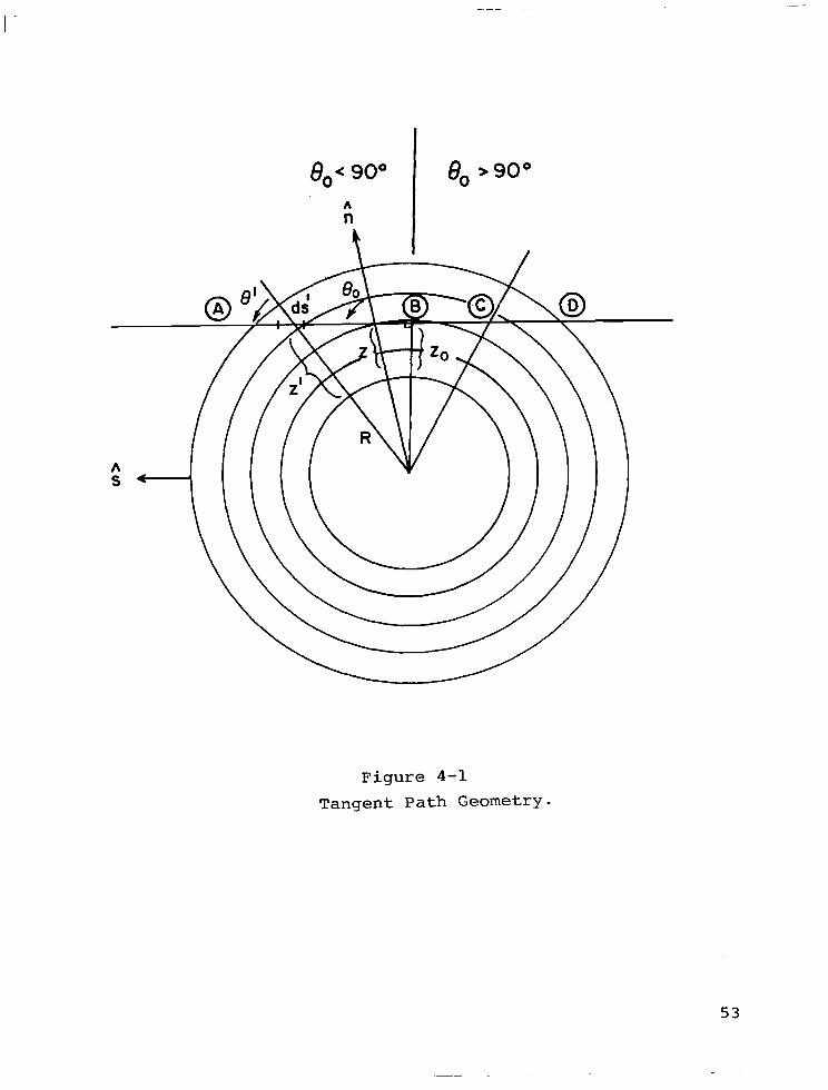
For grazing incidence (values of 8, approaching and
greater than 900), the geometry of the problem is illus-
trated schematically in Figure 4-l. The atmosphere is
assumed to be spherically symmetric, that is the number
density profiles are of the form:
i n = n'(r) (4-18)
where
r = R+z (4-19)
and R is the planetary radius. (The value of R is assumed
to be 6371 km, the Earth's radius at about 35"N.) Neglect-
ing refraction, from simple geometric considerations:
(R + z) sine, = (R + z') sine' (4-20)
and
ds' = dz' sece' = dz' [l - (e,)2sin2eo]D4 (4-21)
The desired slant column density at z along the path at
solar zenith angle 8, will be [from (4-lo)]:
I OJ .
N=(z,e,) = n'(z')[l - ( s,)2sin2eo]-4dz' (4-22) Z
5 2
--- --.------. ----.. . ..--..-..
go< 9o” 8, >90°
A n
t ,
Figure 4-l
Tangent Path Geometry.
53
-.
Assuming a number density distribution with constant scale 2
height HI:
. nl(z') = n'(z)exp(-z'/H1) (4-23)
and using 0' as the integration variable, (4-22) may be
expressed as:
N’(Z,e,) =
. . n'(z)H' xrsine,
8, sine,
0 csc2e'expx1(1 - sine,)‘del
= nl(z)HIM1 sp (0,) (4-24)
where Ch(X' ,e,) is the Chapman (1931) function and the
parameter Xi is:
X1 = (R + z)/Hi (4-25)
This expression has been tabulated by Wilkes (1954) and is
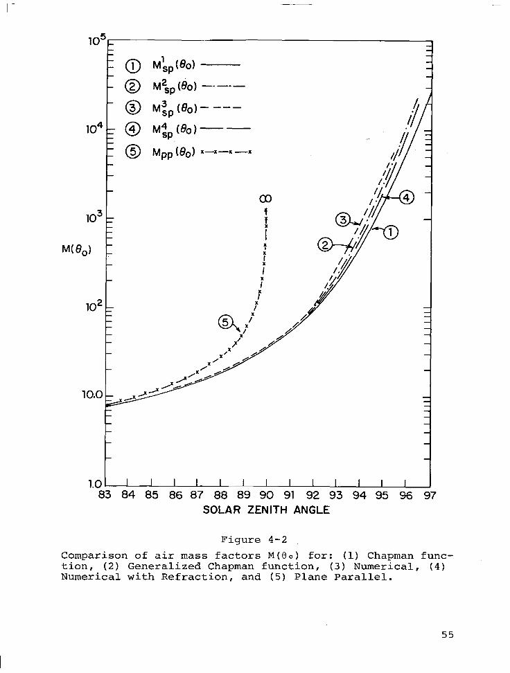
valid for 8, < 90'. Figure 4-2 compares the Chapman
function Mip(io) with the plane-parallel air mass factor
(i.e., sece,) Mpp (6,) for a uniformly mixed gas (02 or M).
M$p(eo) assumes a constant scale height equal to 8.0 km.
For 8, > 900, the Chapman function has been analytically
extended using (see Figure 4-l):
N1(z,eo>900 ,@+Q, = 2Ni(zo,eo=90~,@+@)
(4-26)
-Ni(z,180-8.,0-t@ )
although this approach is not appropriate as discussed by
Swider (1964). 1 Note that MRp and MSp diverge as 8,
approaches 90". From equation (4-16) the slant path
optical depth may be expressed as:
54
0 1 h&p (80)
0 2 M$& (80) -----
0 3 h/lip (80, - ---
0 4 rqp(Bo)--
0 5 Mpp (80) x-x-x-x
1.0 I I I I- I I I I I I I I I 83 84 85 86 87 88 89 90 91 92 93
SOLAR ZENITH ANGLE 94 95 96 97
Figure 4-2
Comparison of air mass factors M(Bo) for: (1) Chapman func- tion, (2) Generalized Chapman function, (3) Numerical, (4) Numerical with Refraction, and (5) Plane Parallel.
55
K. . yz,e,) = c T: Ch(X=,B,) . 1
(4-27)
with appropriate choice of X1. Extensions to the Chapman
function include work by Swider (1964) who investigated
atmospheres with scale height gradients and Green and
Martin (1966) who generalized the analysis for various
density distributions.
4.3.4 Other Analytical Treatments
Swider (1964) noted that in the terrestrial atmosphere
scale height variations with altitude occur and values of
the Chapman function are most sensitive to parameters
(scale heights and number densities) near the lowest
altitude level encountered along the appropriate ray path.
For zenith angles greater than 90", this level is near the
grazing altitude (or tangent height) z, (see Figure 4-l).
By incorporating these considerations simplified approxi-
mations have been derived by numerous authors including
those by Smith and Smith (1972) from the work of Swider
(1964) and Fitzmaurice (1964). For 8, 5 90':
Mgp(z,eo 2 9o”) = i$
(5 Xz) i2
exp(y ) erfc y1 (4-28)
Noting that M&(z,B, = 90°) '" (; xy relation equation
(4-27) can be used to derive an expression for 6, > 90°:
i
M;p(Z'eo i2
, goo) = (; x6,+-& W-2 - n+Wy 1 z z
(4-29)
erfc y']
i where: no = number density at tangent height z,
i n = Z
number density at level z
56
H; = scale height at tangent height
H; = scale height at level z
x; = (R+zo) /d
x; = (R+z) /Hi
and erfc = complimentary error function (=l-erf).
Expression (4-29) accounts for scale height variability in
a realistic terrestrial atmosphere. Figure 4-2 compares
air mass factors M 2 SP
as a function of solar zenith angle
with the constant scale height Chapman function. %p was
evaluated using the scale height and total number density
profiles of the U.S. Standard Atmosphere (1976).
4.3.5 Numerical Forms (including refractive effects)
Slant path column density Nl(z,e,) [and hence air mass
M(z,e,)] may be explicitly evaluated by numerical integra-
tion of the line integral in equation (4-10) along the
appropriate ray path. Advantages offered by this approach
include capabilities to: (a) incorporate realistic number
density profiles, n'(s'), for each species, and (b) include
the effects of refraction within the atmosphere.
Arbitrary number density profiles may be incorporated
into the analysis by integrating equation (4-22) with
suitable quadrature for a specified profile n'(z') taken as
a series of concentric locally homogeneous shells. The
resultant air mass factor Mzp(OO) using the number density
profile cited above is also illustrated in Figure 4-2. For
comparison, previously discussed air mass factors are also
provided.
The effect of refraction on optical path for zenith
angles, 8, > 900, is schematically illustrated in Figure
57
4-3. In the absence of refraction, the appropriate optical
path integral is along (b) at tangent height z,, for rays
reaching altitude z at astronomical zenith angle, 8,. The
unrefracted tangent height is simply determined geometri-
cally:
z, = (E + z)sin(180-8,) - R (4-30)
for 8, > 900. With refraction, the apparent angle of
arrival is e: and the minimum height of the refracted ray
is z:. For monotonically decreasing density profiles the
minimum height of the refracted path is always greater than
that for the unrefracted path, Snider (1975):
1 zo - zo > 0 (4-31)
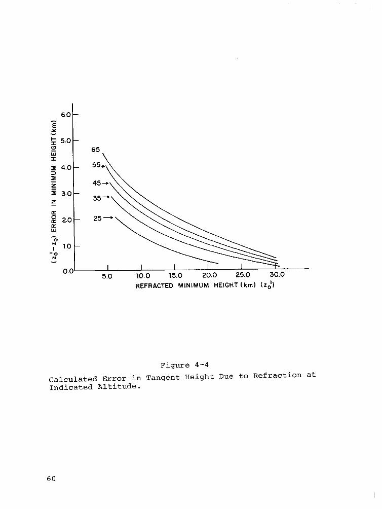
Sample calculations of the error in the minimum height due
to refraction equation (4-31) performed using the procedure
described in Appendix B are shown in Figure 4-4 for values
of z = 25, 35, 45, 55, 65 km. Note that the error is
greatest for high altitudes at large zenith angles (low
minimum heights). Since the column density for 8, > 90° is
most sensitive to the relevant number density near the
tangent altitude [no, see equation (4-29)], the effect of
refraction is to decrease the air mass. Neglecting refrac-
tion, therefore, causes air mass to be overestimated
(Snider, 1975).
Calculations of refracted air mass factor M4 ,,(e,) follow a procedure based on Selby and McClatchey (1972).
Essentially, equation (4-22) is modified by a factor
dependent on the phase refractive index of air, m(z) with
the resultant air mass factor given by (see Appendix B):
58
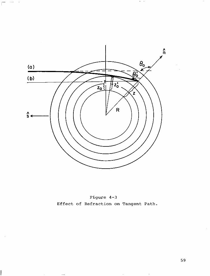
w (b)
Figure 4-3
Effect of Refraction on Tangent Path.
59
6.0 -
z
g 5.0 - c3 iz I 5 4.0 - 3 I z 5 3.0- z
g a 2.0 - E ^o 7 1.0 -
-0 N
65
REFRACTED MINIMUM HEIGHT (km) (2:)
Figure 4-4
Calculated Error in Tangent Height Due to Refraction at Indicated Altitude.
60
2 (R+z')m(z') 1
(4-32)
sin200 -'dz'
Results based on the procedure detailed in Appendix B are
also illustrated in Figure 4-2. Note that the refracted
air mass is less than that for a realistic profile ignoring
refraction (i.e., M3 Sp)' This error for selected angles is
given in Table 4-1. The error increases markedly for large
solar zenith angles.
4.3.6 Summary
The differences among the various spherical approaches
illustrated in Figure 4-2 is not as striking as that
between the plane-parallel and spherical treatments. To
avoid time consuming line integrals and yet retain the
scale height dependence of the true atmosphere we have
retained the Mgp(O,,) approach (which is intermediate in
value). As applied to model calculations of solar beam
extinction, optical paths are evaluated using equation
(4-16)such that:
K -rA(z,O,) = C I? Mi(z,6,)
i=l v (4-33)
where Mi(z,8,) = sec0, 80 < 80'=
Mi(z,&) = Mgp(&,) 8, > 80° -
In the current treatment three species (i.e., sources
of extinction) are handled (i.e., K=3): 02, 03, and
Rayleigh scattering (M). Appropriate choices of scale
height and number density profiles are used in (4-28, 4-29)
depending on whether air mass factors for (02, M) or 03 are
61
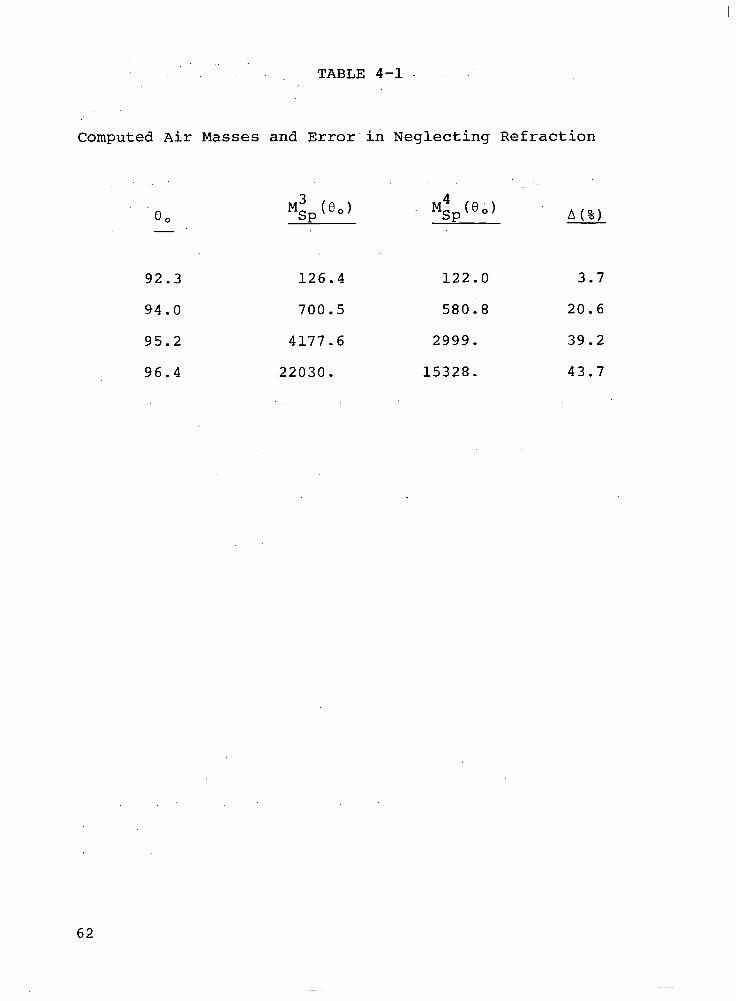
TABLE 4-1
Computed Air Masses and Error‘h Neglecting Refraction
8, -
Mip (eo> M;pteb) A(%)
92.3 126.4 122.0 3.7
94.0 700.5 580.8 20.6
95.2 4177.6 2999. 39.2
96.4 22030. 15328. 43.7
62
being calculated. Thus, the transmission function in a
spherical shell atmosphere TX sp(z,eo) [an alogous to equation
(4-7)] becomes:
Typ(z,EIO) = exp -[Z! ri &(z,e,)] . i=l v
(4-34)
and the dissociative flux due to attenuation (including
scattering of the direct solar bean (but excluding multiply
scattered contributions) is :
Fd&’ = x FA T;PWL) (4-35)
For ozone, a similar approach is adopted (valid above
25 km) modifying the ozone scale height to be equal to 2/3
the ambient pressure scale height. This assumption, is
based on a simple first order ozone profile determined by
photochemical equilibrium. Calculations indicate an error
of less than 5 percent down to 30 km using this approach
(see Fig. 4-5).
4.4 Treatment of Multiple Scattering in the Spherical Shell Geometry
4.4.1 The General Problem
Solutions presented in the previous section (equations
4-34, 4-35) neglect contributions to the dissociative flux
due to the scattered or diffuse intensity. field. at a given
level. To include multiply.,scatto:red radiation in the
spherical shell geometry, the radiative transfer equation
(4-5) must be treated with appropriate definition of the -- --
(Q-V) operator and source function JX(r,R). While the
problem of multiple scattering in spherical shell atmos-
pheres has been treated in the study of steller interiors
(cf. Chandrasekhar, 1960) the, problem is somewhat simpler
~-.- ..-. ..- . -..-. . - .._ . . . . . , _ , , ,
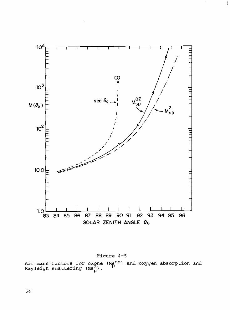
M
104- I I I I I I I I I I ,
1.0 i 83
I I I I I I I I I 84 85 86 87 88 89 90 91 92
SOLAR ZENITH ANGLE 80 93 94 95 96
Figure 4-5
Air mass factors for ozone Rayleigh scattering (MS:).
(MS '
Oz) and oxygen absorption and
64
in that case since both the source function and atmosphere
have spherical symmetry. In the present context however,
the spherical shell atmosphere is externally illuminated by
plane-parallel radiation and overall symmetry is lost.
Thus, while it is relatively straightforward to write down
the relevant form of the radiative transfer equation (see
Fymat, 19771, methods of solution may be tedious.
An examination of alternative approaches to the prob-
lem indicates three general methodologies:
(a) Monte Carlo - (Collins and Wells, 1965; Marchuk and Mikhailov, 1967; Antyufeyev and Nazaraliyev, 1973)
(b) the DART method - (Whitney et al. 1973; Whitney, 1977; Whitney and Malshow, 1977)
(cl approximate semi-
analytical methods-(Shettle and Green, 1974; Sobolev, 1975).
Considerations of computational efficiency for radiative
transfer schemes incorporated within the diurnal photo-
chemical model severely constrain the applicability of
approaches (a) and (b). Therefore, approximate semi-
analytical techniques have been investigated. They may
provide viable alternative methods of solution, especially
when potential errors are assessed relative to other
photochemical model uncertainties. One such approach is
the "locally plane-parallel" (LPP) approximation explored
by Sobolev (1975).
4.4.2 Locally Plane-Parallel Approximation
The conventional plane-parallel (PP) approximation
assumes a plane-parallel atmosphere uniformly illuminated
by a plane-parallel source. As an approximate approach to
treating the general spherical shell problem it may be
assumed that the atmosphere consists of plane-parallel
65
layers (locally), illuminated locally, however, accounting
for the spherical shell nature of the atmosphere (Sobolev,
1975). This procedure relaxes one of the assumptions of
the plane-parallel approximation and should provide results
with reasonable accuracy. Fundamentally, the methodology
requires calculations of the primary source function for
scattering exactly (that is, accounting for Earth curva-
ture) and approximating multiple scattering using the PP
approximation.
By adopting the LPP approach, equation (4-5) becomes
(wavelength suffix omitted):
aI c0se a-r (be) = Ihe) - J(-r,6) (4-36)
where 8 is the local zenith angle and -r(z) is the total
vertical optical depth to altitude z given by:
K. T(Z) = 1 7:(2)
i=l (4-37)
The source function at altitude T(Z) is given by?'
(4-38)
where 1-1 is the cosine of the zenith angle (case), W,(T) is
the single scattering albedo given by:
W,(T) = (4-39)
i- This form and subsequent results assume isotropic scattering. Anderson and Meier (1979) have demonstrated that isotropic scattering provides a qood approximation to Rayleigh multiple scattering solutions throughout the wavelength range .28-.80 urn.
66
where aR is the Rayleigh (molecular) scattering cross-
section (Penndorf, 1957), n M is the total number density,
and J,(T) is the primary source function:
Job) = u"~T' FT [~(Z),e,l (4-40)
Profiles of optical depth and single scattering albedo vs
altitude at dissociative wavelengths are illustrated in
Figures 4-6 and 4-7, respectively.
The primary source function describes the planetary
illumination source. In the plane-parallel approximation,
T is given by equation (4-7) or:
(4-41)
In the LPP approach, the transmission function is defined
by the spherical air mass factors described in the previous
section [equation (4-34)] and:
(d-42)
4.4.3 Method of Solution
A variety of techniques are available to solve equa-
tions (4-36) and (4-38) using the spherical source function
equation (4-42) in the LLP approximation to obtain the
intensity field, Ix, and ultimately the dissociative flux,
Fd A' through equation (4-4). The approach chosen for this
application treats the single integral equation of the
Fredholm type obtainable from equations (4-36) and (4-38)
by suitable transformation (Busbridge, 1960):
-r*
J(-r) = fJJ0 (T) J,(T) + 2 /
0 El+=-t()J(t)dt (4-43)
67
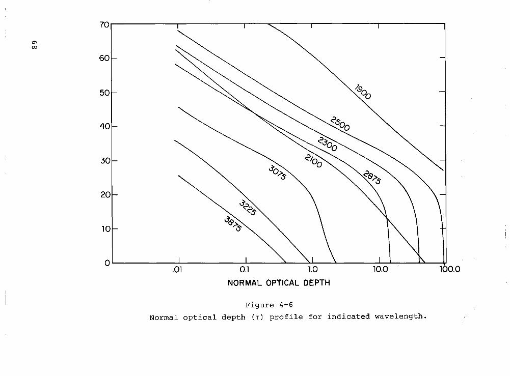
I \
I I
40
30
20-
10-
n
NORMAL OPTICAL DEPTH
Figure 4-6
Normal optical depth (T) profile for indicated wavelength.
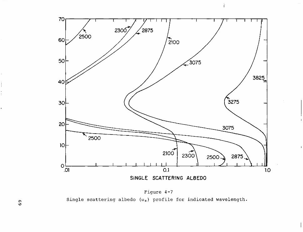
70 I I I I I I I I I I
2875 I / I
k 2500
.Ol 0.1
SINGLE SCATTERING ALBEDO
Figure 4-7
Single scattering albedo (w,) profile for indicated wavelength.
where El is the first exponential integral (see Appendix C)
with general form:
/
‘1
E,(x) = ,-X/P
1-I n-2dp 0
(4-44)
and 'I* is the total normal optical depth [i.e., T* =
T (z=O) 1. When Lambert surface reflection of both the
direct beam and scattered intensity field is included in
the formulation, the integral equation for the source
function becomes:
J(-r) = wo (‘cl J,(T) + 2 /
0
J(t) El( -r-t ) dt
(4-45)
/ -l*
+ RE2(~* --cl [2 c0se,J, (T*)+ W,(T) J(t) 0
where R is the surface albedo. The required dissociative
flux is immediately available noting:
FdE-r (~1 1 = w 0
I;tzj 1
or alternatively:
J[-c (z) 1 (4-46)
/ -l* Fdrr) = FTb,eo) + 2 /
0 J(t)E1( lT-tj)dt
+ 2RE2(~* 9) [coseoFT(-c*,eo)
'c*
+ 2 / 0
J(t)E2(T*-t)dt]
(4-47)
where T[-c(z),B,] is the spherical transmission function
70
given by equation (4-34). The four terms in equation
(4-47) above represent contributions to the dissociative
flux due to: (a) attenuation of the direct solar beam,
(b) the angle integrated diffuse (scattered) intensity
field, (c) surface reflection of the attenuated direct
solar beam, and (d) reflection of the surface incident
angle integrated diffuse intensity field.
Since the source function J(T), is proportional to the
single scatter albedo, w,(-r), [see equations (4-38), and
(4-40)], the dissociative flux equation (4-47) reduces to
the absorption only cases [equations (4-6), and (4-35)]
when the albedo is identically zero (i.e., when there is no
scattering).+
Solution of equation (4-45) is possible using a
variety of techniques including variational methods (Sze,
1976) and iterative techniques (Irvine, 1965). Iterative
techniques such as successive orders of scattering (SOS)
are attractive since they easily accommodate the inhomogen-
eous nature of the atmosphere (as evidenced by the depend-
ence of single scattering albedo on altitude shown in
Fig. 4-7) and provide physical insight into the relative
roles of single vs higher order scattering in determining
dissociative fluxes. Furthermore, if only a few orders of
scattering are required to reach a reasonable solution, SOS
approaches may be computationally competitive with other
multiple scattering treatments SOS calculations converge
rapidly to the desired accuracy for small values of single
scattering albedo since the n th order scattering contribu-
tion to the source function is proportional to U! (Lenoble,
1977). Convergence slows as the albedo approaches unity
t With the exception of the surface reflected term which was not included in the previous development.
71
(very weak absorption) and computational times become
prohibitive as total optical depths, T*, become large
(Nagel et al. 1978).
Examination of Fig. 4-7 suggests that the magnitude of
the single scattering albedo will be small (~0.2) at
altitudes greater than approximately 15 km for dissociative
wavelengths ~3100 i. Alternatively, when albedos approach
unity (generally for X > 3400 %, optical depths are
generally less than 1.0 (see Fig. 4-6). Based on these
observations an SOS treatment has been adopted to evaluate
multiply scattered dissociative fluxes within the wave-
length region of interest.
4.4.4 Single Scattering Results
The first order effects of molecular scattering within
the spherical shell atmosphere are due to single scatter-
ing. Since single scattering calculations are relatively
straight-forward, it is of considerable interest to examine
the degree of accuracy (compared to multiple scattering)
obtainable by considering single scattering alone.
Equation (4-45) is quite amenable to a single scatter-
ing treatment by replacing the full source function, J,
appearing in the integral terms with the primary term, Jo
[equation (4-40)] alone. In the single scattering approxi-
mation:
‘c*
Fd(T,T*,eo,R) = F-h-r, 0,) + % / 0
f,(t)El( t--c )dt
(4-48)
'c* + RE2(-r* -T) [2c0seoT(~*,eo) + I
0 fo (t) E2 (T*-t) dtl)
where
f, (t) = w,(t)T(t,B,) (4-49)
72
and T[~(z),e,] is the transmission function.
Expression (4-48) is near analytical with the require-
ment that two integrals be evaluated. An efficient quadra-
ture technique was developed using piecewise continuous
functions and exploiting the recursion relation for expon-
ential (En) functions to evaluate the integral terms in
equation (4-48) (see Appendix C).
Figures 4-8 and 4-9 summarize sample calculations of
normalized dissociative fluxes (i.e., Fd/F) at wavelengths
of 3475 i and surface albedo 0.2 and 3075 i, R = 0.0,
respectively, for a solar zenith angle of 60°. Curve (1)
[dotted] is the result for absorption only, curve (3) is
the corresponding multiple scattering (MS) result from
Luther and Gelinas (1976). Curve (2) is the single
scattering result consisting of components (a,b,c,d)
corresponding to the four terms in equation (4-48) above:
(a) the attenuated direct solar beam, (b) the singly-
scattered diffuse flux, (c) the surface-reflected direct
solar beam, and (d) the surface-reflected singly scattered
diffuse flux. At 3475 i there is virtually complete
transmission at all altitudes for a purely absorbing atmos-
phere. Therefore, consideration of scattering has a marked
effect on the dissociative flux profile. Examining the
individual contributions to the singly scattered dissocia-
tive flux (curve 2) in comparison to the MS result (curve 3),
it is noted that the shape of the MS flux profile is largely
determined by enhanced extinction of the direct solar beam
to scattering in the lower atmosphere (curve a). As noted
by Lacis and Hansen (1974), the lower atmosphere back-
scatters a fraction of incident solar flux (curve b) to the
upper atmosphere in a manner analogous to an effective
surface reflection. Contributions due to surface reflection
(curves c and d) are significant mainly in the lower atmos-
phere (z < 10 km). Above 20 km, the SS flux profile
73
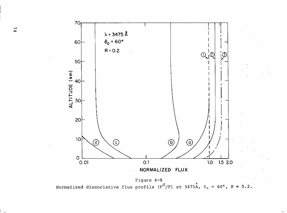
70
60
50
z - 40 ii
z 5 30 a
20
10
0
I
x= 3475Ii
8, = 60”
R=0.2
0.01 0.1 1.0 1.5 2.0
NORMALIZED FLUX
Figure 4-8
Normalized dissociative flux profile (Fd/F) at 3475;, 8, = 60°, R = 0.2.
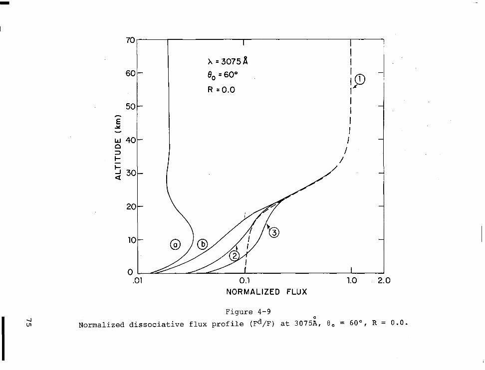
70 r I I
h=3075a
8, = 60”
R =O.O
I I I I I
/ /
.Ol 0.1 1.0 2.0 NORMALIZED FLUX
Figure 4-9
Normalized dissociative flux profile (Fd/F) at 3075;, 8, = 60°, R = 0.0.
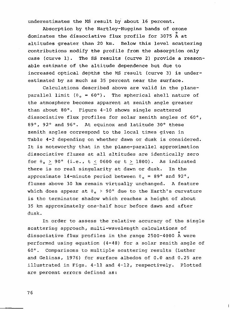
underestimates the MS result by about 16 percent.
Absorption by the Hartley-Huggins bands of ozone
dominates the dissociative flux profile for 3075 g at
altitudes greater than 20 km. Below this level scattering
contributions modify the profile from the absorption only
case (curve 1). The SS results (curve 2) provide a reason-
able estimate of the altitude dependence but due to
increased optical depths the MS result (curve 3) is under-
estimated by as much as 35 percent near the surface.
Calculations described above are valid in the plane-
parallel limit (6, = 600). The spherical shell nature of
the atmosphere becomes apparent at zenith angle greater
than about 80°. Figure 4-10 shows single scattered
dissociative flux profiles for solar zenith angles of 60°,
89', 92O and 96". At equinox and latitude 30° these
zenith angles correspond to the local times given in
Table 4-2 depending on whether dawn or dusk is considered.
It is noteworthy that in the plane-parallel approximation
dissociative fluxes at all altitudes are identically zero
for 8, > 90° (i.e., t < 0600 or t > 1800). As indicated - - - there is no real singularity at dawn or dusk. In the
approximate l4-minute period between 8, = 89' and 92",
fluxes above 30 km remain virtually unchanged. A feature
which does appear at 8, > 90° due to the Earth's curvature
is the terminator shadow which reaches a height of about
35 km approximately one-half hour before dawn and after
dusk.
In order to assess the relative accuracy of the single
scattering approach, multi-wavelength calculations of
dissociative flux profiles in the range 2500-4000 i were
performed using equation (4-48) for a solar zenith angle of
60°. Comparisons to multiple scattering results (Luther
and Gelinas, 1976) for surface albedos of 0.0 and 0.25 are
illustrated in Figs. 4-11 and 4-12, respectively. Plotted
are percent errors defined as:
76
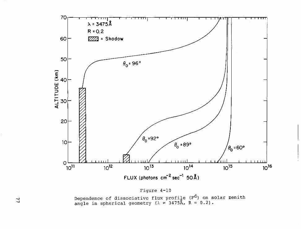
70 I 1 I11111 I I 11111, I I 111111~ I IIll x = 3475%
R =0.2 60
50
m = Shadow
FLUX (photons ctf2sec-’ 50%)
Figure 4-10
Dependence of dissociative flux profiie (Fd) on solar zenith angle in spherical geometry (X = 3475A, R = 0.2).
Solar Zenith
Angle
60
89
90
92
96
TABLE 4-2
Corresponding Local Times (hr)
Dawn Dusk Hours Hours
0821 1539
0605 1755
0600 1800
0551 1809
0532 1828
78
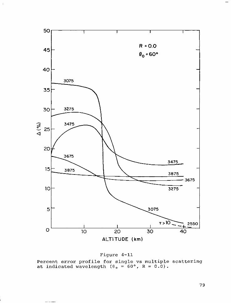
-
50
45
40
35
30
% % 25
20
15
1c
5
0
R =O.O
8, = 60”
3075
3275
I 255
ALTITUDE (km)
Figure 4-11
Percent error profile for single vs multiple scattering at indicated wavelength (8, = 60°, R = 0.0).
79
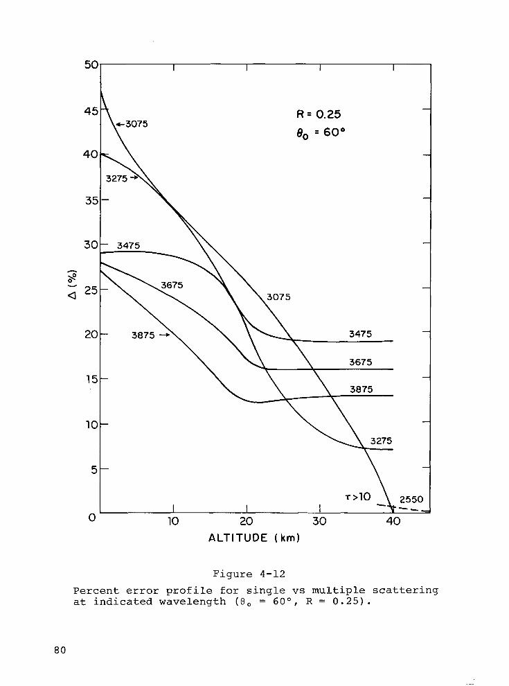
50
45
40
35
30
20
15
10
5
0
I I I I
t -3075
3875 +\ \ \-
R = 0.25
e. = 60”
255C I I I -I
10 20 ALTITUDE (km)
Figure 4-12
30
Percent error profile for single vs multiple scattering at indicated wavelength (0, = 60°, R = 0.25).
80
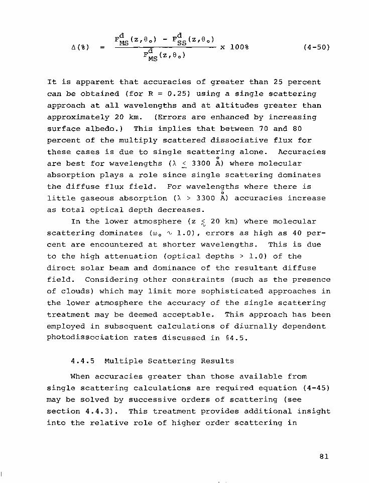
A(%). = F&(Z,eo) - F&(Z,Bo)
Fd x 100% (4-50)
Ms(z’eO)
It is apparent that accuracies of greater than 25 percent
can be obtained (for R = 0.25) using a single scattering
approach at all wavelengths and at altitudes greater than
approximately 20 km. (Errors are enhanced by increasing
surface albedo.) This implies that between 70 and 80
percent of the multiply scattered dissociative flux for
these cases is due to single scattering alone. Accuracies
are best for wavelengths (X < 3300 i) where molecular - absorption p1ays.a role since single scattering dominates
the diffuse flux field. For wavelengths where there is
little gaseous absorption (X > 3300 $ accuracies increase
as total optical depth decreases.
In the lower atmosphere (z $ 20 km) where molecular
scattering dominates (w, % l.O), errors as high as 40 per-
cent are encountered at shorter wavelengths. This is due
to the high attenuation (optical depths > 1.0) of the
direct solar beam and dominance of the resultant diffuse
field. Considering other constraints (such as the presence
of clouds) which may limit more sophisticated approaches in
the lower atmosphere the accuracy of the single scattering
treatment may be deemed acceptable. This approach has been
employed in subsequent calculations of diurnally dependent
photodissociation rates discussed in §4.5.
4.4.5 Multiple Scattering Results
When accuracies greater than those available from
single scattering calculations are required equation (4-45)
may be solved by successive orders of scattering (see
section 4.4.3). This treatment provides additional insight
into the relative role of higher order scattering in
81
determining the dissociative flux profile.
The dissociative flux due to (n + 1) th order scatter-
ing is evaluated by generalizing equation (4-47) :
Tc* F;++) = Ff (be,) + 2 I
0 J,(t&( l-r-tbdt
(4-51) T*
+ 2R E2(~ *-T)[c~s~,F~(T*,B,) + 2 0
Jn(t)E2(T*-t)dt]
where
&Leo) = FT(-r,Bo)
and
J,(T) = w";T) F;(7,Go)
(4-52)
(4-53)
For example, the first order (single) scattering solution
[equation (4-48)] corresponds to n = 0.
Trial calculations based on equation (4-51) are illus-
trated in Fig. 4-13 for a wavelength of 3475 i, solar
zenith angle of 60" and surface albedo of 0.25. At this
wavelength the single scattering albedo profile is near
unity throughout the atmosphere (Fig. 4-7) and the total
optical depth is about 0.6 (Fig. 4-6). Based on these
optical parameters, calculations in this wavelength region
represent a worse case situation for multiple scattering,
i.e., one where the contributions to the dissociative flux
due to multiple scattering are maximum, especially in the
lower atmosphere. It is instructive, therefore, to ascer-
tain the order of scattering required to achieve the
multiple scattering result for this constraining case and
the improved accuracy (with respect to multiple scattering)
incurred with each successive order of scattering. Conver-
gence to the multiple scattering solution (within 0.5%)
82
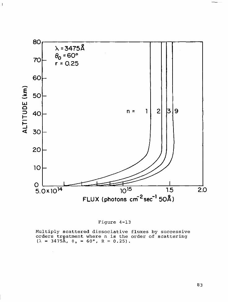
80
70
60
E 5 50
ii z 40
5 Q 30
20
10
0 5.ox1o’4
x = 3475A 8, = 60” r = 0.25
n= 1 2 39
1o15 1.5 FLUX (photons cri*sec-’ 5Oh
Figure 4-13
Multiply scattered dissociative fluxes by successive orders tqatment where n is the order of scattering (A = 3475A, 8, = 60°, R = 0.25).
83
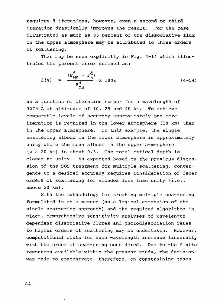
requires 9 iterations, however, even a second or third
iteration drastically improves the result. For the case
illustrated as much as 95 percent of the dissociative flux
in the upper atmosphere may be attributed to three orders
of scattering.
This may be seen explicitly in Fig. 4-14 which illus-
trates the percent error defined as:
A(%) = (FL - FE) F&i
x 100% (4-54)
as a function of iteration number for a wavelength of
3275 i at altitudes of 10, 25 and 40 km. To achieve
comparable levels of accuracy approximately one more
iteration is required in the lower atmosphere (10 km) than
in the upper atmosphere. In this example, the single
scattering albedo in the lower atmosphere is approximately
unity while the mean albedo in the upper atmosphere
(z > 20 km) is about 0.5. The total optical depth is
closer to unity. As expected based on the previous discus-
sion of the SOS treatment for multiple scattering, conver-
gence to a desired accuracy requires consideration of fewer
orders of scattering for albedos less than unity (i.e.,
above 20 km).
With the methodology for treating multiple scattering
formulated in this manner (as a logical extension of the
single scattering approach) and the required algorithms in
place, comprehensive sensitivity analyses of wavelength
dependent dissociative fluxes and photodissociation rates
to higher orders of scattering may be undertaken. However,
computational costs for each wavelength increase linearally
with the order of scattering considered. Due to the finite
resources available within the present study, the decision
was made to concentrate, therefore, on constraining cases
84
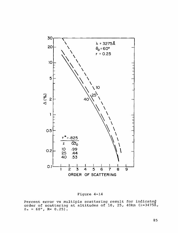
30
20
10
5
52 a
1
0.5
0.2
0.1
\ ~\
\ \
\
\ \
\ \
\ \‘O
X = 3275ii go = 60° r = 0.25
r* = -825
1 23456789 ORDER OF SCATTER I NG
Figure 4-14
Percent error vs multiple scattering result for indicateg order of scattering at altitudes of 10, 25, 40km (X=3475A, 00 = 60°, R= 0.25).
85
such as those described above. For similar reasons,
results presented in subsequent sections are based on
terminating the multiple scattering code after one itera-
tion. As previously discussed, this insures accuracies in
dissociative fluxes on the order of 20-30 percent through-
out most of the atmosphere above the tropopause.
4.5 Application to Diurnally Dependent Photodissociation Rates
As a prerequisite to calculation of diurnal variations
of radical species in the spherical shell geometry, techni-
ques described above were applied to evaluation of photo-
dissociation rates. Single-scattered dissociative fluxes
[equation (4-48)] were computed as a function of wave-
length, altitude, and solar zenith angle (time of day) and
corresponding dissociation rates were evaluated using
equation (4-3) and appropriate cross-section data. Table
4-3 lists the set of dissociative reactions treated in the
analysis. For example, Fig. 4-15 illustrates the vertical
profile of the ratio of single scattered (SS) dissociation
rate to that for pure absorption for reaction 11 in Table
4-3 evaluated at a solar zenith angle of 45O and surface
albedo of 0.2. For comparison, multiple scattering (MS)
results are presented obtained using a variational approach
to solve equation (4-45) (Sze, 1976). Multiple scattering
results for a slightly higher surface albedo (R = 0.25) are
also included (Luther et al. 1978). Results indicate that
single scattering accounts for 75-85 percent of the total
(i.e., MS) photodissociation rate in the upper atmosphere
(z > 20 km).
The difference between plane-parallel and spherical
shell geometries is highlighted by examining variation of
computed photodissociation rates at times near the local
terminator. Figure 4-16 shows the rates for reactions 11
and 20 in Table 4-3 at altitudes of 25 and 40 km near dusk.
86
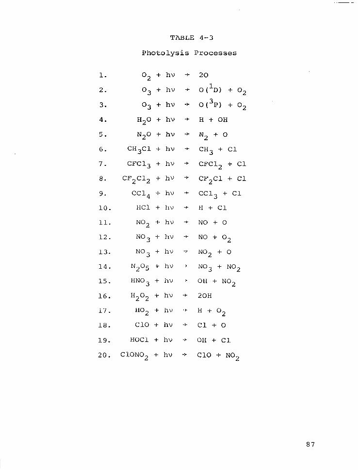
1.
2.
3.
4.
5.
6.
7.
8.
9.
10.
11.
12.
13.
14.
15.
16.
1-1 .
18.
19.
20.
Photolysis Processes
O2 + hv
O3 + hv
O3 + hv
H20 + hv
N20 f hv
CH3Cl + hv
CFC13 f hv
CF2C12 + hv
CC14 -I- hv
HC1 + hv
N02 + hv
N03 + hv
N03 + hv
N205 + hv
HN03 -t hv
H202 -t hv
"O2 -I- I-IV
Cl0 f hv
HOC1 + hv
ClONO, + hv
TABLE 4-3
20
O('D) + O2
o(3P) + o2
H + OH
N2 + 0
CH3 + Cl
CFC12 + Cl
CF2C1 + Cl
ccl3 + Cl
H + Cl
NO + 0
NO + O2
NO2 + 0
N03 + NO2
OH -I- NO2
20H
H + O2
Cl + 0
OH + Cl.
Cl0 + NO.,
87
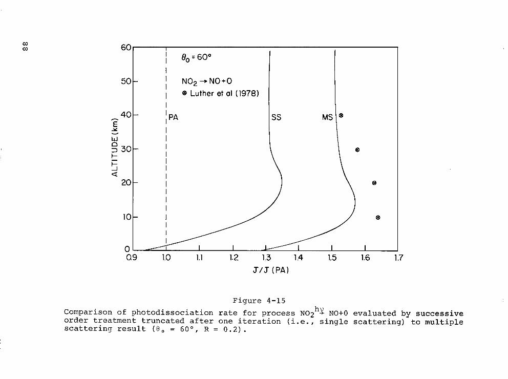
co cu 60
50
40 z E 3 30 l- 5 a
20
10
0
I I I 8,=60°
I I I
NO2 + NO+0
I @ Luther et al (1978) I
; PA ss MS
1.2 1.3 1.4 1.5 1.6 1.7 J/J (PA)
Figure 4-15 Comparison of photodissociation rate for process N02hy NO+0 evaluated by successive order treatment truncated after one iteration (i.e., scattering result (0, = 60°, R = 0.2).
single scattering) to multiple
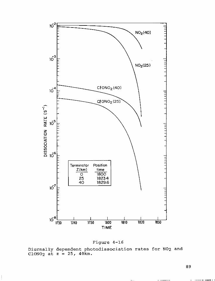
Terminator Position
1081 I I I I I I 1730 1740 1750 1800 1810 1820 1830
TIME
Figure 4-16
Diurnally dependent photodissociation rates for NO2 and ClON02 at z = 25, 40km.
As indicated in the inset, sunset at the surface occurs at
1800 for the case considered (equinox; 30O'latitude). In
the plane-parallel treatment, photodissociation rates at
all altitudes become identically zero at this time. As
indicated by the terminator position times for 25 and 40 km
(1823.4 and 1829.6, respectively), the first order effect
of sphericity at elevations above the surface is to extend
the length of the day. t This amounts to about 3/4 and 1
hour, respectively, at 25 and 40 km (due to dawn/dusk
symmetry).
4.6 Diurnal Calculations
Time dependent altitude profiles of free radical
species (e.g., ClO, ClON02, HCl, H202, H02, OH, NO, N02)
were obtained by performing diurnal calculations using
numerical procedures described in Appendix D. Photodissoc-
iation rates used in the diurnal simulations included:
(a) molecular scattering effects, (b) surface reflection
(a surface albedo of 0.2 was used throughout the wavelength
region) and (c) consideration of the spherical shell geo-
metry of the Earth's atmosphere. Treatment of these
factors has been discussed in previous sections. Single
scattered dissociative fluxes were employed as a first
order treated. As noted above (§4.5) this approximation
accounts for the bulk of molecular scattering within the
wavelength interval. In conducting the diurnal calcula-
tions, long-lived species (such as N20, 03, CH4, etc.) were
held fixed and vertical transport was neglected.
Figures 4-17a and b illustrate time dependent results
for ClON02, OH, N02, Cl0 and H02. An altitude of 40 km was
chosen for demonstration purposes. The solid species
t These times neglect refraction.
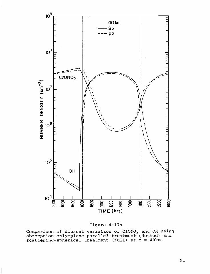
lo8
- m
‘g lo7 Y
E z
k
Efi lo6 z z
lo5
104 : :
CPON02
OH \
\ \
\ \
\ .
40 km -SP --- PP
TIME (hrs)
Figure 4-17a
Comparison of diurnal variation of ClONO2 and OH using absorption only-plane parallel treatment (dotted) and scattering-spherical treatment (full) at z = 40km.
91
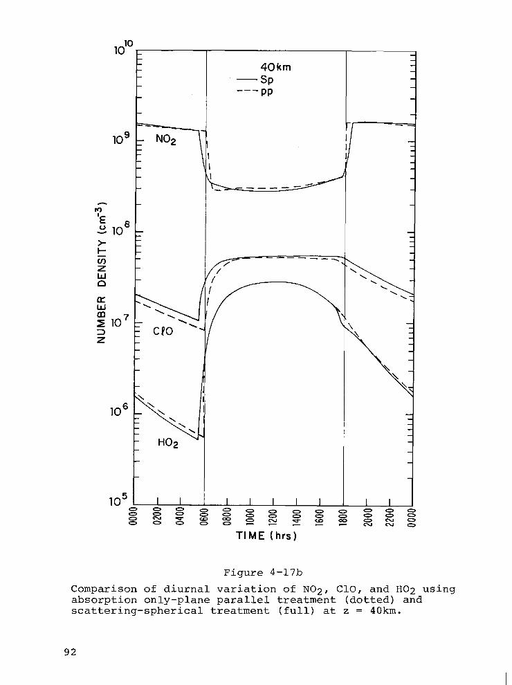
log
h ‘?
E lo8 -
r" lo7 3
I
I I
106 I
.
lo5 I I I I I I I 0” z w 0” 0” 0 0
8 z z E 5 8 2 So---E.
40km -SP ---PP
TIME (hrs)
Figure 4-17b
Comparison of diurnal variation of N02, ClO, and HO2 using absorption only-plane parallel treatment (dotted) and scattering-spherical treatment (full) at z = 40km.
92
abundance curves refer to the spherical shell (Sp), single
scattering result. For comparison, plane-parallel (PP),
pure absorption results (dotted curves) are also provided.
The time scale refers to local time at equinox and 30“
north latitude. Times of dawn (0600) and dusk (1800) at
the surface (z-o km) i- are indicated by light vertical
lines.
4.6.1 Role of Sphericity
Comparing the two sets of results, the gross effect of
sphericity on the diurnal variation of free radical abund-
ances is to accelerate the onset of photochemical produc-
tion (of OH, Cl0 and H02) and loss (of C10N02 and N02) at
dawn and delay termination of these processes at dusk by
approximately one-half hour. Thus, at 40 km sphericity
effectively increases the length of the day by about an
hour (neglecting refraction). Since many photolysis
processes have time constants of seconds to minutes,
specification of precise local dawn and dusk (i.e., at
altitude) is of considerable interest for determining the
transition times between daytime and nighttime chemistries.
As a consequence of these "phase" lags, the plane-
parallel approach may seriously miscalculate abundances of
photochemically active species in the dawn/dusk transition
period. A case in point is the dawn OH concentration
(Fig. 4-17a). In the plane-parallel treatment this is a
nighttime value, however, when Earth curvature is consider-
ed the atmosphere at this time is already about one-half
into daylight and the corresponding OH concentration is two
orders of magnitude higher. The result is not as striking
for Cl0 (Fig. 4-17b) whose major source (photolysis of
t Or at all altitudes in the plane-parallel approximation.
93
ClONO2) has a longer lifetime.
Several gross features of the diurnal variation of
those species illustrated in the figures are worth noting.
These include: (a) the marked difference between daytime
and nighttime species abundances alluded to above (some-
times varying by orders of magnitude), (b) the relatively
slow variation of concentrations with time during mid-day
and nighttime hours, (c) the contrasting rapid variation
during the post-dawn/dusk transition periods and (d) the
absence of symmetry about local noon (1200 hr).
These properties may be understood by considering the
dependence of modeled abundances on the presence of key
photolysis processes during the day, their absence at
night, and the rapid variation of the primary source of
dissociative flux (the Sun) during dawn/dusk transitionary
periods. The relative constancy of concentrations near
midday validates the uses of steady state simulation
approaches for many applications. One aspect which may not
be immediately intuitive is the daily asymmetry with
respect to noontime values. Although photodiss+ociation
rates (which to first order are functions of solar zenith
angle only) are symmetric about noon, photolysis processes
must compete with other production and loss mechanisms
which do not necessarily "follow the Sun". Post-dawn and
post-dusk time dependence is characteristic of the locally
dominant chemistry and thus, distinctive time constants
contribute to the post-dusk apparent log linear behavior.
The attributes discussed above with respect to Figures
4-17a,b are evidently dependent on the particular species
under discussion, however, additional calculations indicate
that they also depend on altitude.
4.6.2 Role of Molecular Scattering
The near noontime values shown in Figs. 4-17a and b
94
provide a calibration point on the relative role of
scattering. For these times of day, the present calcula-
tions reduce to the plane-parallel case and the only
difference between solid and dotted curves is the treatment
of first order scattering in the former case. As illus-
trated, the difference between the two calculations is not
appreciable. However, the magnitude and sign of the con-
centration difference near noon is consistent with other
calculations of the effect of multiple scattering (Luther
et al. 1978). At this altitude (40 km) consideration of
scattering appears to be of minor consequence, however,
additional calculations indicate that the effect is
appreciable at lower altitudes. This behavior is under-
standable upon examination of individual contributions to'
the relevant dissociative fluxes (see Figs. 4-8, 4-9;
§4.4.4). They suggest that the attenuated direct solar
beam dominates in the upper atmosphere while diffuse
contributions become progressively more important toward
the troposphere (i.e., within 2-3 pressure scale heights of
the surface).
4.7 Implications for Remote Sensix
Previous sections have described a methodology for
including the effects of Earth curvature and molecular
scattering in the simulation of diurnally dependent free
radical species concentrations. Ultimately, the utility
of extensions to existing theory may be evaluated based on
their application to either the interpretation of new
measurements or existing data inconsistent with previous
theory. In this section implications of the work described
above are discussed with reference to emerging measurement
techniques based on remote sensing.
Historically, most relevant species profile data have
been collected during daylight hours. This choice is
95
based in part on logistical constraints and in part to take
advantage of the relative constancy of species concentra-
tions during mid-day. Such data sets obviate the need for
other than steady state modeling for most practical
purposes.
Requirements for global monitoring of stratospheric
trace species have motivated recent developments in remote
sensing technology including use of the solar occultation
approach (Russell and Drayson, 1972; Russell et al., 1977;
Chu and McCormick, 1979; Menzies, 1979). An inherent
characteristic of the experimental configuration in this
technique is a sensor field of view with line of sight
integrating across the terminator. As illustrated in the
previous section, the number densities of photochemically
active species may vary by orders of magnitude during dawn
and dusk. It is evident from these results that since
there is such a radical time rate of change, photochemical
equilibrium (i.e., steady state) models may introduce
uncertainties in the interpretation of data obtained by
such techniques.
In principal, most inversion methods for obtaining
vertical species profiles from occultation data such as
analytical treatments (Roble and Hays, 1972) and the onion
peel approach (McKee et al., 1969) rely on the assumption
of spherical symmetry and stratification in the distribu-
tion of the relevant absorbers. Since lines of sight in
the occultation mode essentially look through varying local
times and altitudes, this requires that observed species
are time invariants (i.e., depend on altitude only). The
gross features of the diurnal calculations described in
§5.6 suggest that this is not true for many radical
species. Qualitatively, it is expected that inversion
results based on spherical symmetry considerations will be
least affected for individual species with suppressed
96
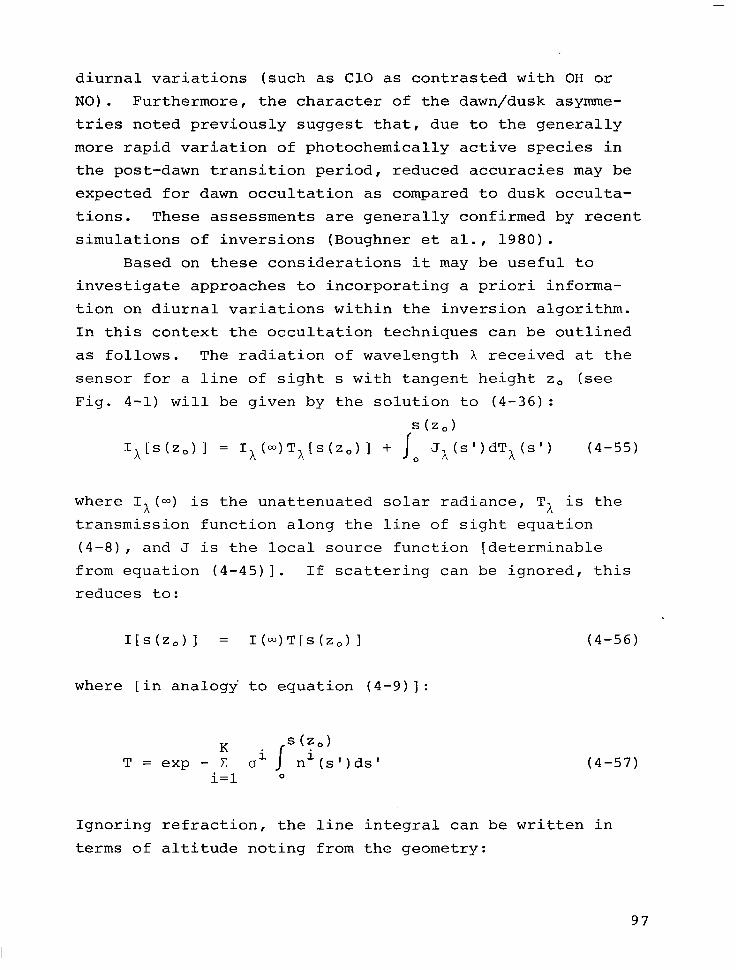
diurnal variations (such as Cl0 as contrasted with OH or
NO) . Furthermore, the character of the dawn/dusk asymme-
tries noted previously suggest that, due to the generally
more rapid variation of photochemically active species in
the post-dawn transition period, reduced accuracies may be
expected for dawn occultation as compared to dusk occulta-
tions. These assessments are generally confirmed by recent
simulations of inversions (Boughner et al., 1980).
Based on these considerations it may be useful to
investigate approaches to incorporating a priori informa-
tion on diurnal variations within the inversion algorithm.
In this context the occultation techniques can be outlined
as follows. The radiation of wavelength X received at the
sensor for a line of sight s with tangent height z, (see
Fig. 4-l) will be given by the solution to (4-36):
s(z,)
IA[s(z,) 1 = Ix@==)Tx[s(zo) 1 + I 0 JA(s')dTA(s') (4-55)
where Ix(") is the unattenuated solar radiance, TA is the
transmission function along the line of sight equation
(d-81, and J is the local source function [determinable
from equation (4-45)]. If scattering can be ignored, this
reduces to:
Iis 3 = I(m)T[s(z,) I (4-56)
where [in analogy to equation (4-g)]:
(4-57) K..
I s (z,)
T=exp-Z 0' n'(s')ds' i=l 0
Ignoring refraction, the line integral can be written in
terms of altitude noting from the geometry:
97
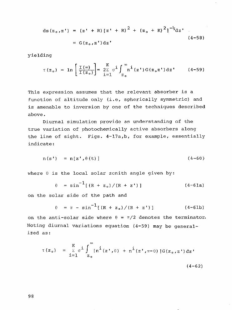
ds(z,,z') = (z' + R)[z' + R) 2 + (z, + RI*1 -%dz 1
(4-58) = G(z,,z')dz'
yielding
T(z,) = ln[~~;',]= :~lci~z~ni(zV)G(zOzV)dzU (4-59)
This expression assumes that the relevant absorber is a
function of altitude only (i.e, spherically symmetric) and
is amenable to inversion by one of the techniques described
above.
Diurnal simulation provide an understanding of the
true variation of photochemically active absorbers along
the line of sight. Figs. 4-17a,b, for example, essentially
indicate:
n(s’) = n[z',O(t)]
where 8 is the local solar zenith angle given by:
0 = sin -1 [(R + zo)/(R + z’) 1
on the solar side of the path and
(4-60)
(4-61a)
0 = n - sin-l[(R + z,)/(R + z')] (4-61b)
on the anti-solar side where 8 = ~r/2 denotes the terminator.
Noting diurnal variations equation (4-59) may be general-
ized as:
K * m . T(z,) = C o1 [n'(z',O) + ni(z',n-e)]G(zO,z')dzl I
i=l zo
(4-62)
98
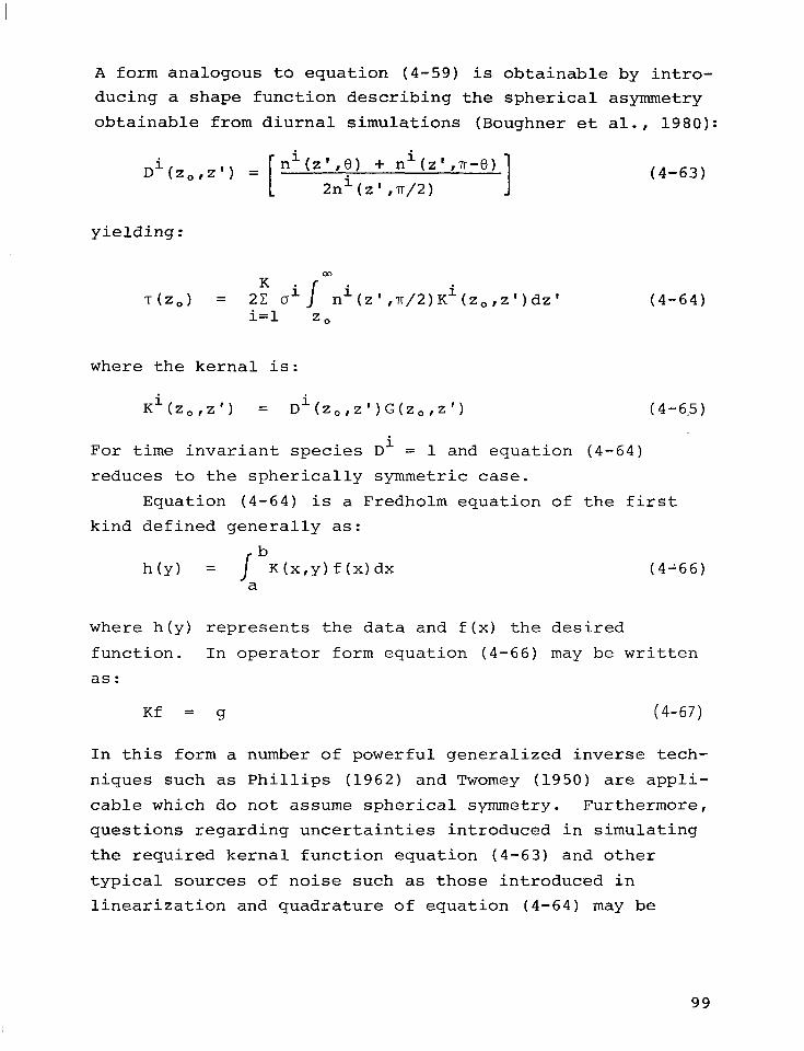
A form analogous to equation (4-59) is obtainable by intro-
ducing a shape function describing the spherical asymmetry
obtainable from diurnal simulations (Boughner et al., 1980):
Di(z orz') = ni(z' ,e) + ni(z' d-8)
2ni(z',7T/2) I
yielding:
T(Z,) = ,~/2)K=(z,,z')dz' i=l z,
(4-63)
(4-64)
where the kernal is:
K=(z orz') = Di(z o,z’)G(zo,z’) (4-63)
For time invariant species Di = 1 and equation (4-64)
reduces to the spherically symmetric case.
Equation (4-64) is a Fredholm equation of the first
kind defined generally as:
b h(y) = / K(x,y)f(x)dx (4166)
a
where h(y) represents the data and f(x) the desired
function. In operator form equation (4-66) may be written
as:
Kf = g (4-67)
In this form a number of powerful generalized inverse tech-
niques such as Phillips (1962) and Twomey (1950) are appli-
cable which do not assume spherical symmetry. Furthermore,
questions regarding uncertainties introduced in simulating
the required kernal function equation (4-63) and other
typical sources of noise such as those introduced in
linearization and quadrature of equation (4-64) may be
99
addressed by examining optimal smoothing parameters,
selecting suitable regularization functions, and employing
appropriate inversion constraints (such as non-negativity).
100
5. SUMMARY AND RECOMMENDATIONS
This section summarizes some of the major findings of
the tasks described in the previous sections. The reader
is referred to the individual sections for more detailed
description of results.
5.1 Model Sensitivity Studies
As discussed in Section 2 the results of 1-D model
simulated ozone perturbations to high altitude aircraft
operations are subject to major uncertainties particularly
as regards rate constant data related to OH chemistry.
Sensitivity studies indicate that calculated OH concentra-
tion profiles are most sensitive to values adopted for the
reactions listed in Table 2-l. Perturbation calculations
were performed for three model scenarios corresponding to
high (model A) and low (models B and C) values of strato-
spheric OH concentration. Model C investigates the poten-
tial role of peroxynitric acid (H02N02) as a sink for OH
and provides indicators of OH concentration (e.g., ClO,
HNO3/N02, HF/HCl) in best agreement with measurements.
Model A tends to predict an increase in column ozone for
both low (15 km) and high (20 km) NO, injections. The low
OH models (B and C), however, predict a small (~1%) increase
for the low altitude injection, but a fairly significant
reduction for the high altitude case (-5.5%, model C). More reliable kinetic data is needed to differentiate between
the models discussed.
Additionally, it is noted that injection of NO, may
perturb both local stratospheric and surface temperatures.
Thus, climatic changes should be considered in addition to
column ozone perturbations.
101
5.2 Two-Dimensional Zonal-Mean Modeling
The application of Eulerian averaging processes to
zonal-mean models introduces a number of undesirable
features associated with the eddy flux contributions to
transport. The feasibility of some kind of Lagrangian
approach as an alternative averaging methodology is attrac-
tive from the standpoint that eddy terms are avoided.
However, difficulties arise in the implementation of the
formulation and in interpretation of mixing ratio results
in comparison with observations. Several areas are identi-
fied for additional research before the Generalized Lagran-
gian Mean (GLM) tracer equation may be applied to zonal
modeling.
In the short term, numerical tracer experiments compar-
ing Eulerian and GLM approaches may be performed deriving
the required Lagrangian velocity components for given three-
dimensional motion fields. One potential avenue for
research would concentrate on cases with small disturbances
using a more precise treatment of the diabatic heating rate
to generate Lagrangian velocity fields.
Longer term research may be profitably directed to
examining the interpretation of the basic continuity equa-
tion and in reformulating the momentum equation by defining
more generalized differential operators.
5.3 Remote Sensing
The role of multiple scattering and Earth sphericity
on the calculation of diurnally dependent photodissociation
rates and trace species concentrations was examined in
Section 4 with particular emphasis on dawn and dusk.
Calculations of slant path air mass factors indicated
that sphericity should be considered in evaluating the
primary source function for scattering for solar zenith
angles greater than about 80°. Evaluation of profiles of
102
atmospheric optical depth and single scatter albedo at dis-
sociative wavelengths suggested that a successive order of
scattering (SOS) approach may be viable at all altitudes.
A locally plane-parallel (LPP) treatment of the radiative
transfer equation was adopted to treat the spherical geom-
etry. Comparison of single scattered dissociative flux
profiles with multiple scattering results indicated that
between 70 and 80 percent of multiply scattered flux above
20 km can be accounted for by single scattering alone. In
the lower atmosphere where molecular scattering dominates
errors as high as 40 percent are encountered, however,
accuracies comparable to those in the upper atmosphere can
be achieved by considering an additional order of scatter-
ing. Convergence to the multiple scattering result (within
0.5%) requires about 9 orders of scattering, however,
5 percent accuracy is available in the upper (lower) atmos-
phere with only 3 (4) orders. Diurnal calculations of
trace species indicate that the gross effect of sphericity
on diurnal variation is to accelerate the onset of photoly-
tic processes at "plane-parallel" dawn and delay their
termination at "plane-parallel" dusk.
Based on the results of diurnal trace species varia-
tion across the terminator region, it is recommended that a
potential approach to the inversion problem in the occulta-
tion geometry may be consideration of generalized inverse
techniques not relying on assumptions of spherical symmetry.
In this manner the shape of the kernel function may be
estimated to first order using a priori calculations of
diurnal trace species concentrations.
103
APPENDIX A
Earth-Sun Geometry
As in the plane-parallel case, the transmission path
for solar radiation incident at a specified altitude, z(km),
will be a function of the local solar zenith angle, 8,.
The solar zenith angle may be defined from the scalar
product of the local surface normal vector, A, and the
Sun's direction vector, s. In a celestial coordinate
system with origin fixed at the Earth's center, the unit
normal vector will be a function of latitude, X, and local
hour angle, HA. The unit solar direction vector, s^, will
depend on the Sun's declination angle, 6. The required
relationship between solar zenith angle, latitude, solar
declination angle and hour angle is given by:
case, = sind sinX + cosd cosX cosHA (A-1)
Solar declination angle, 6, may be approximated as:
sin6 = 0.3978 sin[.9863(d-80)l (A-2 1
where d is the day of the year (1 Jan. = 1, 20 Mar. = 80,
etc.). Note that 6 is zero at the equinoxes, and has
maxima ISI = 23' 27' at the solstices.
The hour angle, HA, is defined as identically zero at
local noon, 1200h, (Sun's direction vector along observer's
meridian) when the Sun's zenith angle is smallest:
case, (1200) = sing sinX + cosd cosX (A-3)
Conversely, sunrise and sunset times may be defined as
corresponding to solar zenith angles of 90'. The length of
the day in hours is then given by:
LOD = &OS -'[-tan6 tanX] (A-4)
104
Thus hour angle may be written as:
HA(deg) = 15(12.00-t) + & (A-5)
where 15 is the Earth's angular rotation rate ("h-1) and E
is a correction for the equation of time. Equations (A-l),
(A-2) and (A-5) define a solar zenith angle for a given
date, time, and latitude.
Additionally, the local normal, A, and the Sun's
direction vector, s, define a plane of incidence pictured
in Fig. (A-l). This plane contains the subsolar point (SSP)
where the solar zenith angle is zero and the required local
normal vector, ii. For solar zenith angles which are
sufficiently small (say 8, < 800), a plane-parallel treat-
ment will suffice. For situations near sunrise and sunset,
however, the Earth's sphericity is a critical consideration.
Figure (A-l) illustrates a number of relevant cases. Local
normal A, denotes a situation with B. approaching 90°. In
this case the usual plane parallel treatment (sece,) will
overestimate the relevant optical path. As illustrated by
local normal fi2, the solar zenith angle 0: may be >90° at
elevations above the surface. For these situations the
upper atmosphere may be illuminated while the lower atmos-
phere is not. The shadow height will be given by:
zs = R(csce, - 1)
= R(secU - 1) (A-6)
where U is the solar depression angle defined as:
e,b900) = 900 + u (A-7)
and R is the Earth's radius (6371x103m). Thus for U = 8O
sunrise occurs at an altitude of 62.6xlOjm. This corres-
ponds to about 0523 local time at equinox at 30°N. [These
calculations and equation (A-6) ignore refractive effects
which decrease Zs.]
105
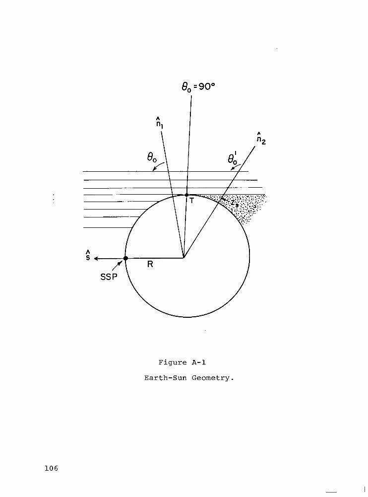
8, = 90”
A
SSP \
Figure A-l
Earth-Sun Geometry.
106
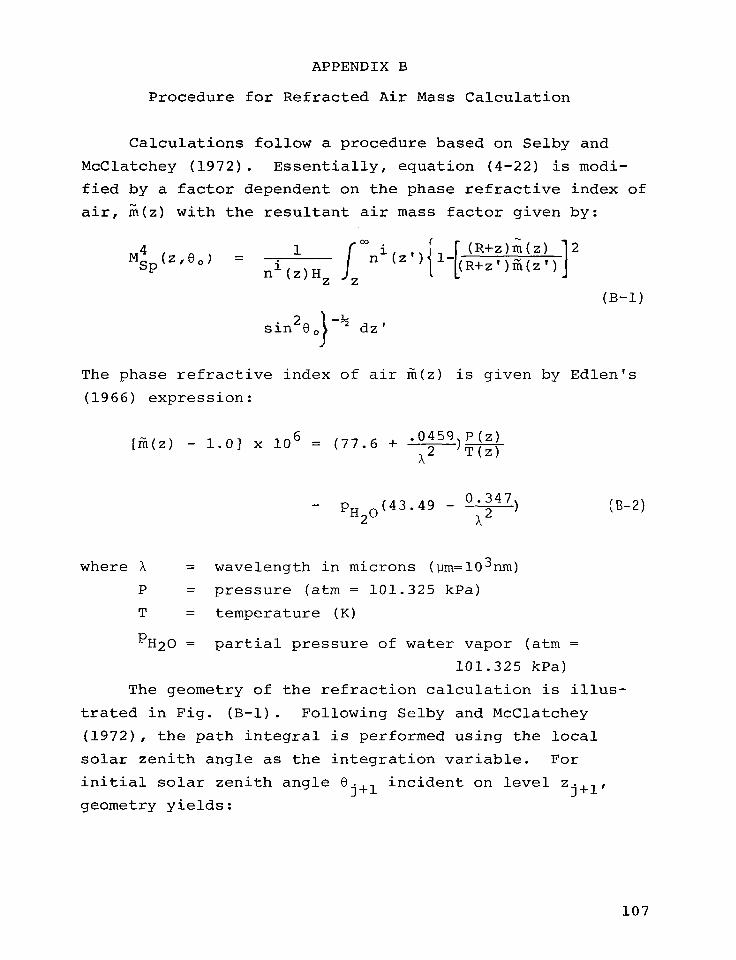
APPENDIX B
Procedure for Refracted Air Mass Calculation
Calculations follow a procedure based on Selby and
McClatchey (1972). Essentially, equation (4-22) is modi-
fied by a factor dependent on the phase refractive index of
air, c(z) with the resultant air mass factor given by:
M;p(z,eol =
(B-1)
sin2eo -si dz'
The phase refractive index of air iii(z) is given by Edlen's
(1966) expression:
[ffii(z) - 1.01 x lo6 = (77.6 + .0459)P(Z) - A2 T(z)
- p, o(43.49 - 01$47) CI (B-2)
where X = wavelength in microns (pm=103nm)
P = pressure (atm = 101.325 kPa)
T = temperature (K)
rH20 = partial pressure of water vapor (atm =
101.325 kPa)
The geometry of the refraction calculation is illus-
trated in Fig. (B-l). Following Selby and McClatchey
(1972), the path integral is performed using the local
solar zenith angle as the integration variable. For
initial solar zenith angle 8. I+1
incident on level z j+l' geometry yields:
107
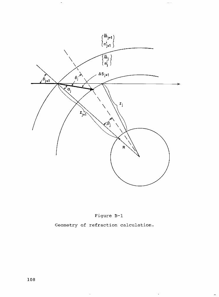
Figure B-l
Geometry of refraction calculation.
108
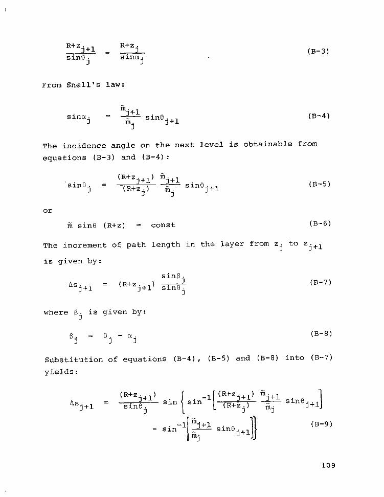
R+Z j+l R+z. =3
sine. sincl. 3 3
From Snell's law:
mj+l sine sina. = _ 3 m.
3 j-l-l
(B-3)
(B-4)
The incidence angle on the next level is obtainable from
equations (B-3) and (B-4):
sine. = (R+Zj+l) ‘j+l
3 (R+zj) mj sinej+l (B-5)
or
fii sine (R+z) = const (B-6)
The increment of path length in the layer from z. to z~+~ 7
is given by:
sin.B . As~+~ = (R+zj+l) ZGG?
j
where 6. 7
is given by:
5 = ej - Y
(B-7)
(B-8)
Substitution of equations (B-4), (B-5) and (B-8) into (B-7)
yields:
As j+l = (R+zj+l) sin sme .
3
_ sin-l mj+l ,
I" ma sme j+l
3 1
(B-9)
109
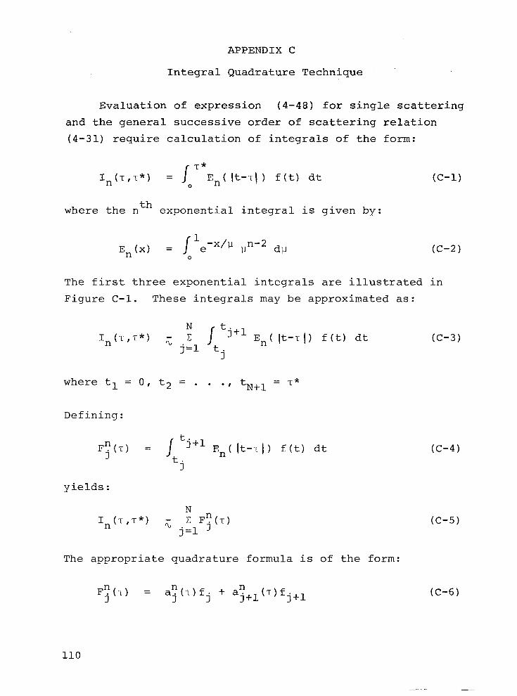
APPENDIX C
Integral Quadrature Technique
Evaluation of expression (4-48) for single scattering
and the general successive order of scattering relation
(4-31) require calculation of integrals of the form:
/ Tc*
In(T,Tc*) = 0
En(!t--r() f(t) dt
where the n th exponential integral is given by:
I 1 En(x) =
e-x/p n-2 u dv
0
(C-1)
(C-2)
The first three exponential integrals are illustrated in
Figure C-l. These integrals may be approximated as:
N
/
t. IJLT**) ; c
j=l t. '+' En( It-T\, f(t) dt
7
where tl = 0, t2 = . . ., tN+l = T*
Defining:
F;(T) = I tj+l
t. EJ It---cl) f(t) dt
7
yields:
N I,hJ*) - C Fn(-c)
'L j=l J
The appropriate quadrature formula is of the form:
F;(T) = ay(T)f. + an 7 J+l(T)fj+l
(C-3)
(C-4)
(C-5)
(C-6)
110
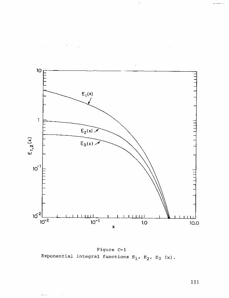
10
1
x - N L
ii-
10-l
I I III1 10.0
Figure C-l Exponential integral functions El, E2, E3 (x).
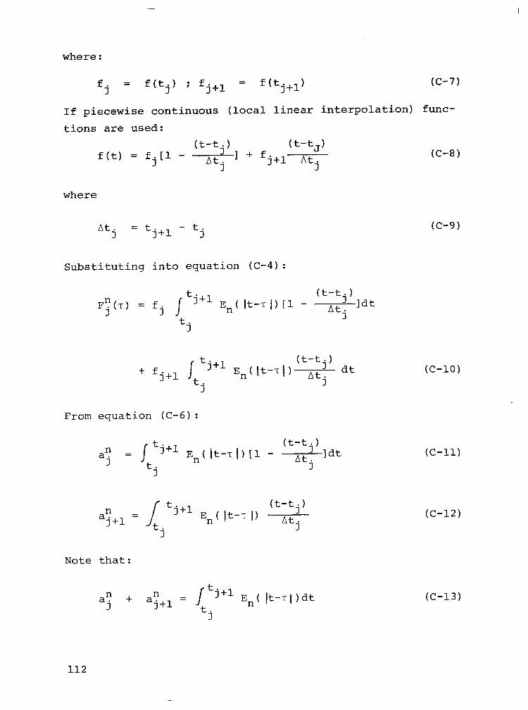
where:
f. 3
= f(tj) ; fj+l = f(tj+l) (C-7)
If piecewise continuous (local linear interpolation) func-
tions are used:
f(t)
(t-tj)
=fj[l- at (t-t,)
j I + fj+l Atj
where
At. = t. - t. 3 I+1 I
Substituting into equation (C-4):
(t-t.) F~(7) = fj
/ tj+l En( It--c 1) [1 - At’ ldt
i t.
-I 3
+ fj+l tj+l (t-tj)
EJlt-+ At dt
j j
From equation (C-6):
(t-t-) n a. = tj+l 7 t.
En( It-T 1) [1 - At3 Id+= 3
j
n /
tj+l (t-tj)
aj+l = t En( It--c 1) At
j j
Note that:
n + n a. aj+l = / tj+l
3 t En( (t--cl)dt
j
(C-8)
(C-9)
(C-10)
(C-11)
(C-12)
(C-13)
112
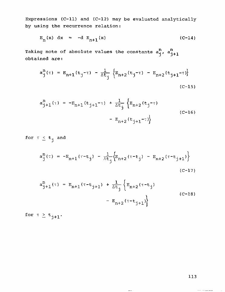
Expressions (C-11) and (C-12) may be evaluated analytically
by using the recurrence relation:
E,(x) dx = -d En+l (xl (C-14)
Taking note of absolute values the constants a;, a? 1+1
obtained are:
a:(T) = En+l('j-~) - & j
En+2 (ti-T) - En+2 (tj+l-7))
(C-15)
n aj+l(T) = -E,+l(tj+l-~) + & j
En+2(tj-T)
(C-16)
- En+2(t. I+1 --T)
for T < t. and - 3
a:(T) = -En++-tj) - & j
(‘-tj) - En+2 (T-tj+l)
(C-17)
n aj+l(T) = En+l(‘-tj+l) + & j
En+2(T-tj)
- En+2(T-t. ,+1)
for 'c 2 tj+l.
(C-18)
113
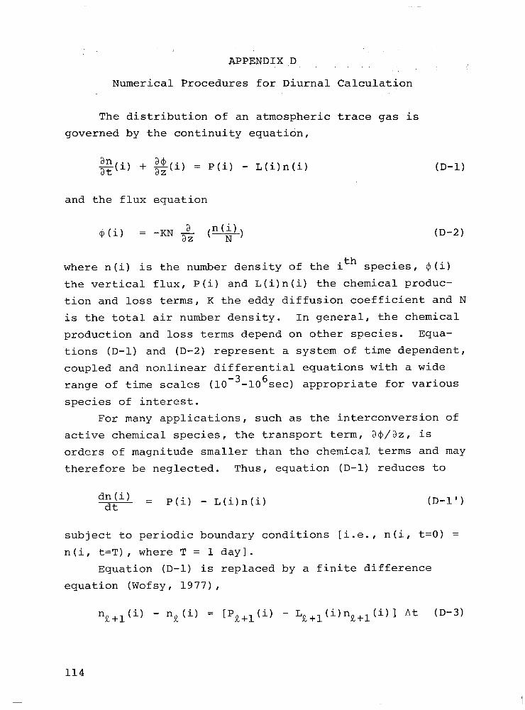
APPENDIX D
Numerical Procedures for Diurnal
The distribution of an atmospheric
governed by the continuity equation,
g(i) + g(i) = P(i) - L(i)n(i)
and the flux equation
$(i) = a -mJ E ( n(i) N 1
where n(i) is the number density of the
Calculation
trace gas is
(D-1)
(D-2)
ith species, e(i)
the vertical flux, P(i) and L(i)n(i) the chemical produc-
tion and loss terms, K the eddy diffusion coefficient and N
is the total air number density. In general, the chemical
production and loss terms depend on other species. Equa-
tions (D-l) and (D-2) represent a system of time dependent,
coupled and nonlinear differential equations with a wide
range of time scales (10 -3 -106sec) appropriate for various
species of interest.
For many applications, such as the interconversion of
active chemical species, the transport term, a$/az, is
orders of magnitude smaller than the chemical terms and may
therefore be neglected. Thus, equation (D-l) reduces to
an(i) = dt P(i) - L(i)n(i) (D-l')
subject to periodic boundary conditions [i.e., n(i, t=O) =
n(i, t=T) , where T = 1 day].
Equation (D-l) is replaced by a finite difference
equation (Wofsy, 1977),
nR+l (i) - n,(i) = [Pa+l(i) - LR+l(i)nt+l(i) 1 At (D-3)
114
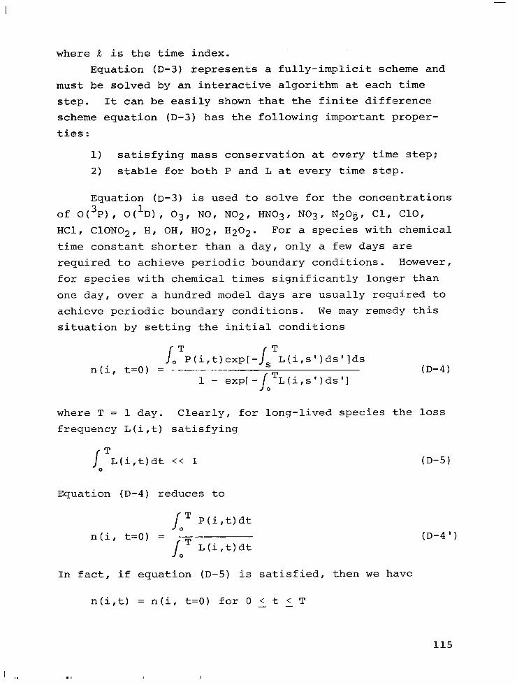
where R is the time index.
Equation (D-3) represents a fully-implicit scheme and
must be solved by an interactive algorithm at each time
step. It can be easily shown that the finite difference
scheme equation (D-3) has the following important proper-
ties:
1) satisfying mass conservation at every time step:
2) stable for both P and L at every time step.
Equation (D-3) is used to solve for the concentrations
of W3W, Oh, 03, NO, N02, HN03, N03, N20+ Cl, ClO,
HCl, C10N02, H, OH, H02, H202. For a species with chemical
time constant shorter than a day, only a few days are
required to achieve periodic boundary conditions. However,
for species with chemical times significantly longer than
one day, over a hundred model days are usually required to
achieve periodic boundary conditions. We may remedy this
situation by setting the initial conditions
n(i,
T P(i,t)exp[- L(i,s')ds']ds
l- exp[ - TL(i,s')ds'] (D-4)
where T = 1 day. Clearly, for long-lived species the loss
frequency L(i,t) satisfying
/ T
L(i,t)dt << 1 0
Equation (D-4) reduces to
J T P(i,t)dt
n(i, t=o) = OT
J L(i,t)dt 0
(D-5)
(D-4')
In fact, if equation (D-5) is satisfied, then we have
n(i,t) = n(i, t=O) for 0 < t < T - -
115
This procedure of adjusting initial conditions at the
beginning of each model day greatly reduces the number of
model days required for relaxation.
116
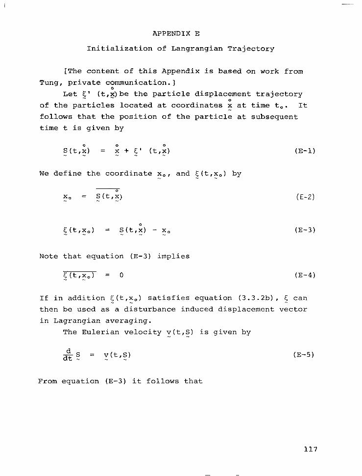
APPENDIX E
Initialization of Langrangian Trajectory
[The content of this Appendix is based on work from
Tung , private communication.]
Let 5' (t,g)be the particle displacement trajectory
of the particles located at coordinates G at time t,. It
follows that the position of the particle at subsequent
time t is given by
S(t,G) = ; + 5' (t,G
We define the coordinate x,, and E(t,x,) by
x, = s G)
gt,+ = S(t,G) - x,
Note that equation (E-3) implies
5(t,x,) = 0
(E-1)
(E-2)
(E-3)
(E-4)
If in addition <(t,x,) satisfies equation (3.3.2b), 5 can
then be used as a disturbance induced displacement vector
in Lagrangian averaging.
The Eulerian velocity v(t,S) is given by
&s = v(t,S) (E-5)
From equation (E-3) it follows that
117
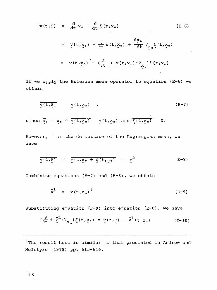
v(t,S) = *X dt .%O + & $(bx,)
a dxo = y(t,xo) + at E(Lxo) + * vxog (t,xo)
= y(t,zo) + ($ + y(t,x,)*Vx )S(t,x,) o-- .-
If we apply the Eulerian mean operator to equation (E-6) we
obtain
v(t,S) = v(t,xo) , (E-7)
since X, = x0 -f v(t,x,) = V(t,x,) and <(t,x,) = 0.
However, from the definition of the Lagrangian mean, we
have
v(t,S) = v(t,xo + S(t,xo) = vL
Combining equations (E-7) and (E-8), we obtain
;L = v(t,xo) t
(E-8)
(E-9)
Substituting equation (E-9) into equation (E-6), we have
a (at+ v
-L.v xo)S(t,xo) = y(W) - SLN,xo) (E-10)
t The result here is similar to that presented in Andrew and
McIntyre (1978) pp. 615-616.
118
which is identical to equation (3.3.2b). Thus, E(t,x,)
can be used for Lagrangian averaging and is directly
related to trajectory motion of the particles.
Note that in the above definition, the GLM operations
depend on the choice of time to at which the particles are
labelled‘by g. In terms of c(t,xo), this is characterized
by the.fact that <(t,,x,) = 0. A different initialization,
i.e., choice of t$ and-g4 can lead to different.averaged
values for some quantities (see McIntyre, 1979).
119
APPENDIX F
High Altitude Aircraft Emissions
As a consequence of projected high altitude aircraft
operations, appreciable quantities of combustion products
of fossil-origin fuels may be emitted into the ambient
atmosphere. Typical aviation fuels consist primarily of
a mixture of higher hydrocarbon petroleum distillates (e.g.,
Jet A - "kerosene', CgH20-C16H34; Jet B - "naptha",
C6H14-C7H16) and inherent residual impurities such as
sulfur and heavy metals. Exhaust product constituents may
be categorized as: (1) products of complete combustion
including water vapor (H20) and carbon dioxide (C02),
(2) products of incomplete combustion including carbon
monoxide (CO) and hydrocarbons (HC), and (3) products due
to residual impurities such as sulfur (S) and its oxides
(SO2), and oxides of nitrogen (NOx). This discussion
focuses on the evaluation of aircraft related yearly source
strengths (MT yr -l) for H20, CO, S and NO,. Total emissions
are dependent both on intrinsic emission characteristics of
individual aircraft/engine configurations as given by the
emission index and fleet related modes of operation includ-
ing total number of aircraft and cruising time per day.
Emissions of individual pollutants and pollutant
groups are quantified in terms of relavant emission indices,
EI, which are the number of grams of pollutant produced for
each kilogram of fuel consumed. In general, EI are depend-
ent on engine type, mode of operation (cruise, idle, etc.),
cruise power setting, flight altitude, and cruising speed.
However, EI have been recommended for typical cruise
conditions for performing atmospheric model calculations
(Grobman and Ingebo, 1974).
An upper limit to the emission index may be evaluated
120
based on stoichiometric considerations assuming perfect
combustion efficiency. For example, for a kerosene mixture
(Jet A), a water vapor emission index EI(H20) of about
1400 g/kg fuel is predicted. Higher order distillates such
as naptha produce slightly higher yields of H20*. Measure-
ments indicate slightly lower values of emission index
(CIAP, 1975) and 1250 g/kg fuel is the recommended value
for cruise conditions and all engine types.
The emission of sulfur, primarily as S02, is deter-
mined by the fuel stock sulfur content which is expressed
as percent by weight, %(w/w). This abundance is controlla-
ble by implementing available fuel desulfurization techni-
ques. Current average aviation fuel sulfur contents are
0.05 percent (w/w) with a maximum allowable value of 0.30
percent (w/w) (CIAP, 1975). These values suggest typical
and worse case EI(S) of 0.5 and 3.0 g/kg fuel, respectively.
Elevated combustion zone temperatures and the presence
of radicals such as 0, N, and OH facilitate the formation
of oxides of nitrogen which would not be energetically
favored under ambient conditions. Since NO, emissions are
highly dependent on operating conditions, values at cruise
conditions are assumed. It is necessary to distinguish
between near term (present day) and far term design con-
cepts in assigning NO, emission indices (Poppoff et al.,
1978) since future technological advances are planned to
reduce NO, emissions by a factor of 6 (Reck, 1978).
* It is notable that H20 emission indices for coal-derived
fuels suggested for implementation in certain advanced SST (ASST) design concepts (Witcofski, 1978) are significantly higher. For example, synthetic liquid natural gas (SYN-LNG) has a EI(H20) of about 2300 g/kg fuel while that for liquid hydrogen (LH2) is near 9000 g/kg fuel. On an energy equiv- alent basis, these emissions are 60 and 160 percent higher, respectively, than Jet A (Witcofski, 1978).
121
Typical near term emissions [EI(NOx) = 18 g/kg fuel] are .' based-on the.Olympus 593 engine as described in Lohmann and
Riecke (1977); this value is consistent with that given by
Grobman and Ingebo (1974). The corresponding far term
technology estimate is 3 g/kg fuel. Values of EI(N0,) are . summarized in Table F-l.
Assessment of potential perturbations to atmospheric
chemistry and global climate due to aircraft exhaust
emissions is dependent on the total fleet-derived source
strength, Ri(MT yr -l) for each pollutant species, which is
defined as
Ri = (EI)iM~Tf/1012 (F-1)
where M is the number of aircraft in the proposed nominal
fleet, @(kg fuel hr -1) the engine fuel flow rate at cruise
altitude and Tf(hr/yr) the yearly cruise time in hours for
each aircraft. Typical source strengths based on the given
emission indices and a nominal fleet of 500 aircraft are
evaluated and presented in Table F-l. In these calcula-
tions, we assume an average engine fuel flow rate of
3.78~10~ kg fuel hr-l, which is based on a "Type A" air-
craft as defined in Poppoff et al. (1978) and described in
Baber and Swanson (1976). Cruise time is taken to be 7 hr
per day per aircraft.
Equivalent aircraft production rates Pa are evaluated
assuming injection of NO, as pure NO+ and distributing it
uniformly over the globe in a 1 km thick spherical shell
(to be centered at the cruise altitudes of 15.2 and
t The assumption of pure NO production is only approximately true. The volume fraction of NO, however, is equal to 90-95 percent (CIAP, 1975) of the total NO, emissions.
122
18.3 km). Based on these assumptions, the given aircraft
characteristics are converted to equivalent production
rates using:
pa = (7.82~10-~)M(EI) (F-2)
Calculations based on equations (F-l) and F-2) for NO, are
summarized in Table.F-2.' Ozone perturbation sensitivity
analysis will be performed on these values.
123
----. ---.-. ..- -. -..-.. . II. I I... .I ,
REFERENCES
Andrew, D.G.,and McIntyre, M.Z. (1978) An Exact Theory of
Non-Linear Waves in a Lagrangian-Mean Flow. z. Fluid
Mech., 89, 609. - -
Anderson, D.E.,and Meier, R.R. (1979) Effects of Anisotro-
pit Multiple Scattering on Solar Radiation in the
Troposphere and Stratosphere. APP~. Optics, 18, 1955. -
Antyufeyev, V-S., and Nazararaliyev, M.A. (1973) A New Modi-
fication of the Monte Carlo Method for Solution of
Problems in the Theory of Light Scattering in Spheri-
cal Atmosphere. Atmos. Oceanic Phys., 2, 463.
Baber, H.T., Jr., and Swanson, E.E. (1976) Advanced Super-
sonic Technology Concept AST-100 Characteristics
Development in a Baseline-Update Study. NASA TM
X-72815.
Borucki, W.J., Whitten, R.C., Watson, V.R., Woodward, H.T.,
Niegel, C.A., Capone, C.A., and Becker, T. (1976)
Model Prediction of Latitude Dependent Ozone Due to
Supersonic Operations. AIAA J., 14, 1738. -- -
Boughner, R., Larsen, J.C., and Natarajan, M. (1980) The
Influence of NO and Cl0 Variations at Twilight or the
Interpretation of Solar Occultation Measurements.
Geophysical e. Letters, \z. 7-, 1%. 4, Apr. 1980,
PP. 231-234.
Buijs, H.L., Vail, G.L., Tremblay, G., and Kendall, D.J.W.
(1980) Measurement of the Volume Mixing Ratios for HCl
and HF in the Stratosphere. Geophysical Res. Letters,
Vol. 7, No. 3, Mar. 1980, pp. 205-208. - - -
124
Busbridge, I.W. (1960) The Mathematics of Radiative Trans-
fer. Cambridge Univ. Press.
Callis, L.B., Ramanathan, V., Boughner, R-E., and
Barkstrom, B.R. (1975) The Stratosphere: Scattering
Effects, A Coupled 1-D Model, and Thermal Balance
Effects. Fourth Conference on CIAP, U.S. DOT, 224-233. -- - .-
Callis, L.B. (1974) The Importance of Rayleigh Scattering
on Photochemical Processes in the Stratosphere. Paper
presented at the 1974 Fall Annual Meeting, Dec. 12-17,
AGU.
Chandrasekhar, S. (1960) Radiative Transfer. Dover.
Chang, J.S. (1976) In Halocarbons: Effects on Stratospher-
ic Ozone. NAS Report, Washington, D.C. -
Chapman, S. (1931) The Absorption and Dissociative or Ion-
izing Effect of Monochromatic Radiation in an Atmos-
phere on a Rotating Earth. II, Grazing Incidence.
Proc. Phys. Sot., 43, 483. _-- - --
Chu, W.P., and McCormick, M.P. (1979) Inversion of Strato-
spheric Aerosol and Gaseous Constituents from
Spacecraft Solar Extinction Data in the .38-1.0 ym
Wavelength Region. APP~. Optics, 18, 1404. -
Collins, D.G., and Wells, M.B. (1965) Monte Carlo Codes for Study of Light Transport in the Atmosphere. Rep. RRA-T54, Vols. 1 and 2, Fort Worth, TX, Radiation
Research Assoc.
Crutzen, P.J. (1971) Ozone Production Rates in an Oxygen-
Hydrogen-Nitrogen Oxide Atmosphere. J. .Gebphvs . Res. , - 76, 7311. -
Crutzen, P.J. (1970) The Influence of Nitrogen Oxides on
the Atmospheric. Ozone Content. Quart. J. Roy. Meteor. -- sot., 96, 320. - -
Danielson, E.F. (1968) Stratospheric-Tropospheric Exchange
Based on Radioactivity, Ozone and Potential Vorticity.
J. Atmos. Sci., 25, 502. - - -
Duewer, W.H., Wuebbles, D.J., Ellsaesser, H.W., and
Chang, J.S. (1977) NO, Catalytic Ozone Destruction:
Sensitivity to Rate Coefficients. J. Geophys. Res., - 82, 935. -
Dunkerton, T. (1978) On the Mean Meridional Mass Motions of
Stratosphere and Mesosphere. J. Atmos. Sci., 35, 2325. - - -
Edlen, B. (1966) Meteorologia, 2, 12.
English, J.M., Oliver, R.C., and Forney, A.K. CIAP (1975)
Propulsion Eggluents in the Stratosphere. DOT TST-75-
52. U.S. Dept. of Transportation.
Evans, W.V., Kerr, J.B., Wardle, D-I., McConnell, J.C.,
Ridley, B.A., and Schiff, H.I. (1976) Intercomparison
of NO, N02, and HN03 Measurements with Photochemical
Theory. Atmosphere, 14, 189. -
Farmer, C.B., and Raper, O.F. (1977) The HF:HCl Ratio in
the 14-38 km Region of the Stratosphere. Geophys. Res.
Lett., 4, 527.
126
Fitzmaurice, J.A. (1964) Simplification of the Chapman
Function for Atmospheric Attenuation. APP~. Optics.,
3, 640.
Fontanella, J.C., Girand, A., Gramont, L.,and Louisnard, N.
(1975) Vertical Distribution of NO, N02, and HN03 As
Derived From Stratospheric Absorption Infrared.Spectra.
Appl. Optics, 14, 825. -- ~- _I
Fymat, A. (1977) Inversion Methods in Temperature. and
Aerosol Remote Sounding: Their Commonality and
Differences, and Some Unexplored Approaches. Inver-
sion Methods in Atmospheric Remote Sounding. A. Deepak
(ea.) Academic Press, 429-463.
Graham, R.A., Winer, A.M., and Pitts, J.N., Jr. (1978)
Pressure and Temperature Dependence of the Unimolec-
ular Decomposition of H02N02. 2. Chem. Phys., 68,
4505.
Green, A.E.S., and Martin, J.D. (1966) Generalized Function
in The Middle Ultraviolet: Its Science and Technology.
A.E.S. Green (ed.) Wiley, 140-157.
Green, J.S.A. (1970) Transfer Properties of Large Scale
Eddies and the General Circulation of the Atmosphere.
Quart. 2. Meteor. s., 96, 157.
Grobecker, A.J., Coronti, S.C., and Cannon, R.H., Jr. CIAP
(1974) The Effects of Stratospheric Pollution by
Aircraft. DOT-TST-75-50, U.S. Dept. of Transportation.
127
Grobman, J., and Ingebo, R.D. (1974) Forecast of Jet-Engine
Exhaust Emissions for Future High Altitude Commercial
Aircraft. Proc. Third Conference on the Climatic
Impact Assessment Program. Rep. No. DOT-TSC-OST-74-15,
U.S. Dept. of Transportation.
Hansen, J.E., and Travis, L.D. (1974) Light Scattering in
Planetary Atmospheres. Space Sci. Rev., 16, 527. - -
Harris, J.E. (1978) Ratio of HN03 to NO2 Concentration in
Daytime Stratosphere. Nature, 274, 235.
Harris, J.E., Moss, D.G., Swann, N.R., Neill, G.F., and
Gildwang, P. (1976) Simultaneous Measurements of H20,
NO2 and HNO-3 in the Daytime Stratosphere From 15 to
35 hm. Nature, 259, 300.
Harris, J.E. (1976) The Distribution of Water Vapor in the
Stratosphere. Rev. Geophys. Space Phys., 14, 565.
Harwood, R.S., and Pyle, J.A. (1977) Studies of the Ozone
Budget Using a Zonal Mean Circulation Model and
Linearized Photochemistry. Quart. 5. Roy. Meteorol.
sot., 103, 319. - -
Harwood, R.S., and Pyle, J.A. (1975) A Two-Dimensional Mean
Circulation Model for the Atmosphere Below 80 km.
Quart. IL. Roy. Meteorol. Sot., 101, 723. - -
Herman, J.R. (1979) The Response of Stratospheric Consti-
tuents to a Solar Eclipse, Sunrise and Sunset.
5. Geophys. g., 84, 3701.
128
Hidalgo, H., and Crutzen, P.J. (19?7) The Tropospheric and
Stratospheric Composition Perturbed by NO, Emissions
of High-Altitude Aircraft. J. Geophys. ., 82, 5833.
Hinds, M.K. (1979) Studies of Residence Times of Chloro-
flurocarbons Using a Two-Dimensional Model. ,_ Meteor.
Msg., 108, 22.
Holton, J.R. (1975) The Dynamics Meteorology of the Strato-
sphere and Mesosphere. Mesosphere. Meteor. Monog.,
15, No. 37. -
Howard, C.J., and Evenson, K.M. (1977) Kinetics of the
Reaction of HO2 with NO. Geophys. Res. Lett., 4, 437. --
Irvine, W.M. (1965) Multiple Scattering by Large Particles.
A_. J., 142, 1563. ---
Johnston, H.S. (1971) Reduction of Stratospheric Ozone by
Nitrogen Oxide Catalysts from Supersonic Transport
Exhaust. Science, 173, 517. --
Kida, H. (1977) A Numerical Investigation of the Strato-
spheric General Circulation and Stratospheric
Tropospheric Mass Exchange, II. Langrangian Motion
of the Atmosphere. J. Meteor. Sot. Japan, 55, 71. - -
Krishnamurti, T.N. .(1961) The Subtropical Jet Stream of
Winter. J. Meteor., 18, 172. - -
Lacis, A.A., and Hansen, J.E. (1974) A Parameterization for
the Absorption of Solar Radiation in the Earth's
Atmosphere. _. J Atmos. Sci., 31, 118. - -
129
_ Lenoble, J. led.) (1977) Standard Procedures to Compu>
__ Atmospheric Radiative Transfer in a Scattering Atmos-
phere. IAMAP, Boulder, CO.
Loewenstein, M., Borucki, W.J., Savage, H.F., Borucki, J.E.,
.and Whitten, R.C. (1978) Geographical Variations of NO
and 03 in the Lower Stratosphere. J. Geophys. Res., - 83, 1875. -
Logan, J-A., Prather, M.J., Wofsy, S.C., and McElroy, M.B.
(1978) Atmospheric Chemistry: Respond to Human Influ-
ence. Trans. Roy. z., 290, 187. Phil.
Lohmann, R.A., and Riecke, G.T. (1977) Analytical Screening
of Low Emissions, High Performance Duct Burners for
Supersonic Cruise Aircraft Engines. NASA CR-135157.
Lorentz, E.N. (1967) The Nature and Theory of the General
Circulation of the Atmosphere. WMO No. 218.
Louis, J.F., London, J., and Danielson, E.F. (1974) The
Interaction of Radiation and Meridional Circulation of
the Stratosphere Proceedings of the IAMAP/IAPSO
Combined First Special Assemblies, Melbourne,
Australia, Vol. II, 1205.
Luther, F.M. (1973) Monthly Mean Values of Eddy Diffusion
Coefficients in the Lower Stratosphere. AIM paper
73, 495. AIAA/AMS Conference, Denver, CO. -
Luther, F.M., and Gelinas, R.J. (1976) Effect of Molecular
Multiple Scattering and Surface Albedo on Atmospheric
Photodissociation Rates. J. Geophys. Res., 81, 1125. -
130
-
Luther, F.M., Wuebbles, D-J., Duewer, W-H., and Change, J.S.
(1978) Effect of Multiple Scattering on Species Concen-
trations and Model Sensitivity. 2. Geophx. Res., 83, -- -- 3563.
Mahlman, JiD. (1975) Some Fundamental Limitations of Simpli-
'fied Transport Model. Proceedings of the Earth CIAP
Conference. Ref. 132. U.S. Dept. of Transportation.
Mahlman, J.D. (1973) On the Maintenance of Polar Front Jet
Stream. J. Atmos. Sci., 30, 544. - - ---
Mahlman, J.D. (1969) Heat Balance and Mean MeridionalCircu-
lation in Polar Stratosphere During Sudden Warmings in
January, 1958. Mon. Wea. Rev., 97, 534. - .- -
Mahlman, J.D., Levy, H., II, and Maxim, W.J. (1980) Three-
Dimensional Traces Structure and Behavior as Simulated
in Two Ozone Precursor Experiments. J. Atmos. Sci., - 37, 655.
Marchuk, G.I., and Mikhailov, G.A. (1967) Results of the
Solution of Some Problems in Atmospheric Optics by a
Monte Carlo Method. Atmos. Oceanic Phys., 2, 227.
Matsuno, T. (1980) Lagrangian Motion of Air Parcels in the
Stratosphere in the Presence of Planetary Waves. Pure
APP~. Geophys., 118, 189.
Matsuno, T., and Nakamura, K. (1979) The Eulerian and
Lagrangian Mean MeridionalCirculations in the Stratos-
phere at Time o'f Sudden Warming. -. J Atmos. Sci., 36, - - 680.
131
McConnell, J.C., and Evans, W.F.J. (1978) Implications of
Low Stratospheric Hydroxyl Concentrations for CFM and
SST Scenario Calculations of Ozone Depletion. EOS
Trans. AGU, 59, 1978. --
McDonald, J. (1971) Presentation Before the Department of
Commerce Technical Advisory Board on Environmental
Aspects of the Supersonic Transport, Boulder, CO.,
March 17-18.
McElroy, M.B., and McConnell, J.C. (1971) Nitrous Oxide:
A Natural Source of Stratospheric NO. 2. Atmos. S&.,
28, 1095. -
McElroy, M.B., Wofsy, S.C., Penner, J.E., and
McConnell, J.C. (1974) Atmosphere Ozone: Possible
Impact of Stratospheric Aviation. J. Atmos. Sci., 31, - - - 287.
McIntyre, M.E. (1979) Towards the Lagrangian Mean Descrip-
tion of Stratospheric Circulation and Chemical Trans-
port. To appear in Phil. Trans. Roy. Sot. A. --
McKee, T.B., Whitman, R.I., and Lambiotte, J.J. (1969) A
Technique to Infer Atmospheric Temperature Using
Horizon Radiance Profiles. NASA TN D-5068.
Menzies, R.T. (1979) Remote Measurements of Cl0 in the
Stratosphere. Geophys. Res. Lett., a, 151. --
Molina, L.T., and Molina, M.J. (1980) UV Absorption of
Cross-Section of H02N02 Vapor. Report to U.S. Dept.
of Trans. High Altitude Pollution Program Rep. No.
FAA-EE-80-07.
132
. . . ..I I I. ..I.I.-.-.....-.--.- . . .----. ..---. -... . . -.-.-.-. .--...-... . ..- . . . . . .._. . _. .._. _..._. - ..-..-.-__. -.- -_--.- ..__ I
-
Murgatroyd, R.J., and Singleton, F.S. (1961) Possible
MeridionalCirculations in Top Stratosphere and Meso-
phere. Quant. J. Meteor. Sot., 87, 125. -- - -.
Nagel, M.R., Quenzel, H., Kweta, W., and Wendling, R. (1978)
Daylight Illumination-Color-Contrast Tables.
Academic Press.
NASA (1979) The Stratosphere: Present and Future.
R.D. Hudson (ea.) NASA Ref. Publ. 1049, NASA Goddard
Space Flight Center.
NASA (1977) Chlorofluoromethanes and the Stratosphere.
NASA RP-1010, Washington, D.C.
Newell, R.A., Wallace, J.M., and Mahaney, J.R. (1966) The
General Circulation of the Atmosphere and its Effects
on the Movement of Trace Substances. II. Tellus, 18, - 363.
Nicolet, M., and Vergison (1971) L'oxyde Azoteux dans la
Straospere. Aeron. Acta., A-91. - -
Oort, A.H., and Rasmussen, E.M. (1971) Atmospheric Circu-
lation Statistics. NOM Prof. Paper 5. National
Oceanic and Atmospheric Administration.
Penndorf, R. (1957) Tables of the Refractive Index for
Standard Air and the Rayleigh Scattering Coefficient
for the Spectral Region Between 0.2 and 20.0 pm and
Their Application to Atmospheric Optics. 2. opt. sot. -~ Am., 47, 176. - -
133
Phillips, D.L. (1962) A Technique for the Numerical Solu-
-tions at Certain Integral Equations of the First Kind.
J. Assoc. Comput. Mach., 2, 97. -
Plumb, R.A. (1979) Eddy Fluxes of Conserved Quantities by
Small Amplitude Waves. J. Atmos. Sci., 36, 1699. - - -
Poppoff, I.G., Whitten, R.C., Turco, R.P., and Capone, L.A.
(1978) An Assessment of the Effects of Supersonic Air-
craft Operations on the Stratospheric Ozone Content.
NASA RP-1026.
Reck, G.M. (1978) In An Assessment of the Effect of Super-
sonic Aircraft Operations on the Stratospheric Ozone
Content. NASA RP-1026.
Reed, R.J., and German, K.E. (1965) A Contribution to the
Problem of Stratospheric Diffusion by Large-Scale
Mixing. Mon. Wea. Rev., 93, 313. ---
Riehl, H., and Fultz, D. (1957) Jet Stream and Large Waves
in a Steady Rotating-Dishpan Experiment: Structure of
the Circulation. Quart. 2. Roy. Meteor. G., 83, 215.
Roble, R.G., and Hays, P.B. (1972) A Technique for Recover-
ing the Vertical Number Density Profile of Atmospheric
Gases from Planetary Occultation Data. Planet. Space
Sci., 20, 1727. - -
Russell, J.M., and Drayson, S.R. (1972) The Influence of
Atmospheric Ozone Using Satellite Horizon Measurements
in the 1042 cm-l Band. J. Atmos. Sci., 29, 376. - - -
134
Russell, J.M., Park, J.H., and Drayson, S.R. (1977) Global
Monitoring of Stratospheric Halogen Compounds from a
Satellite Using Gas Filter Spectroscoping in the Solar
Occultation Mode. Appl. Opt., 16, 607. - -
Sawyer, -J.S. (1965) The Dynamical Problems of the Lower
Stratosphere. Quart. 2.. Roy. Meteor. - _ sot., 91, 407.
Selby, J.E.A., and McClatchey, R.A. (1972) Atmospheric
Transmittance from 0.25 to 28.5 Micrometers: Computer
Code LOWTRAN 2. Tech. Rep. AFCRL-72-0745, Air Force
Geophys. Labs.
Shettle, E.P., and Green, A.E.S. (1974) Multiple Scattering
Calculation of the Middle Ultraviolet Reaching the
Ground. Apol. Opt., l3-, 1967. L -
Smith, F.L., III, and Smith, C. t.1972) Numerical Evaluation
of Chapman's Grazing Incidence Integral Ch(X,x).
J. Geophys. Res., 77, 3592. - -
Snider, D.E. (1975) Refractive Effects in Remote Sensing
of the Atmosphere with Infrared Transmission Spectros-
copy. _. J Atmos ' . g-., 32, 2178.
Sobolev, V.V. (1975) Light Scattering in Planetary Atmos-
pheres. Pergamon Press, NY.
Swider, W., Jr. (1964) The Determination of the Optical
Depth at Large Solar Zenith Distances. Planet Space
Sci., 12, 761.
Sze, N.D. (1976) Variational Methods in Radiative Transfer
Problems. h. Quant. Spectros. Radiat. Trans., 16, 763.
135
Sze, N.D. (1978) Stratospheric Fluorine: A Comparison
Between Theory and Measurements. Geophys. Res. Lett., -- 2, 781.
Sze, N.D., and Ko, M.K.W. (1980) Photochemistry of COS,
-2, CH3Sch3, and H2S: Implications for the Atmospher-
ic Sulfur Cycle. Atmos. Environ., 14, 1223. ,-
Sze, N.D., and Ko, M.K.W. (1979) CS2 and COS in Stratospher-
ic Sulfur Budget. Nature, 280, 308.
Turco, R.P., Whitten, R.C., Poppoff, I.G., and Capone, L.A.
(1978) SSTs, Nitrogen Fertilizer and Stratospheric
Ozone. Nature, 276, 805.
Twomey, S. (1950) On the Numerical Solution of Fredholm
Integral Equations of the First Kind by the Inversion
of the Linear System Produced by Quadrature. J. Assoc. - Comput. Mach., 10, 99.
U.S. Standard Atmospheric Supplement (1966), U.S. Government
Printing Office, Washington, D.C.
Vupputuri, R.K.R. (1973) Numerical Experiments on the
Steady State Meridionalstructure and Ozone Distribu-
tion in the Stratosphere. Mon. Wea. Rev., 101, 510. --- -
Vupputuri, R.K.R. (1979) The Structure of the Natural
Stratosphere and the Impact of Chlorofluromethanes on
the Ozone Layer Investigated in a 2-D Time Dependent
Model. Pure and Appl. Geophys., 117, 448. ---
Wang, W.C., and Sze, N.D. (1980) Coupled Effects of Atmos-
pheric N20 and 03 on the Earth's Climate. Nature,
Vol. 286, 589.
136
Wang, W-C., Yung, Y.L., Lacis, A.A., MO. T., and
Hansen, J.E. (1976) Greenhouse Effects Due to Man-Made
Perturbations of Trace Gases. Science, 194, 685.
Whitney, C. (1977) Extending Radiative Transfer Models by
Use of Bayes' Rule. _. J Atmos. Sci., 34, 766. - --
Whitney, C.K., and Malchow, H.L. (1978) Study of Radiative
Transfer in Scattering Atmosphere. AFGL-TR-78-0101.
Whitney, C.K., Var, R.E., and Gray, C.R. (1973) Research
Into Radiative Transfer Modeling and Applications-
Atmospheric Physics. AFCRL-TR-73-0420.
Whitten, R.C., Borucki, W.J., Watson, V.R., Shimazaki, T.,
Woodward, H.T., Niegel, C.A., Capone, L.A., and
Becker, T. (1977). The NASA Ames Research Center
One- and Two-Dimensional Stratospheric Models. Part 2:
The Two-Dimensional Model. NASA TP-1003.
Widhopf, G.F. (1975) A Two-Dimensional Photochemical Model
of the Stratosphere Including Initial Results of
Inert Tracer Studies. Proc. Fourth Conf. on CIAP.
T. Hand, and A. Broderick (eds.) DOT-TSC-OST-75-38,
316.
Wiin-Neilsen, A., and Sela, J. (1971) On the Transport of
Quasi-Geostrophic Potential Vorticity. Mon. Weath.
Rev., 99, 447. - -
Wilkes, M.V. (1954) A Table of Chapman's Grazing Incidence
Integral Ch(X,x). Proc. Phys. Sot., B67, 304. - - - -
137
Witcofski, R.D. (1978) Progress in Coal Derived Fuels for
Aviation Systems,. NASA TM-78696.
Wofsy, S.C. (1976) Interactions of CH4 and CO in
Earth's Atmosphere. Ann. Rev. Earth Planet -- 441.
the
Sci., 4,
Wofsy, S.C., and McElroy, M.B. (1973) On Vertical Mixing
In the Upper Stratosphere and Lower Mesosphere.
J. - Geophys. Res., 78, 2819. - -
138
1. Report No. 2. Government Accession No.
NASA CR-3410 4. Title and Subtitle
ATMOSPHERIC STUDIES RELATED TO AEROSPACE ACTIVITIES AND REMOTE SENSING TECHNOLOGY
7. Authorls)
N. D. Sze, R. G. Isaacs, M. Ko, and M. B. McElroy
9. Performing Organization Name and Address
3. Recipient’s Catalog No.
5. Report Date
March 1981 6. Performing Organization Code
0. Performing Organration Report No,
10. Work Unit No.
Atmospheric and Environmental Research, Inc. 872 Massachusetts Avenue Cambridge, Massachusetts 02139
12. Sponsoring Agency Name and Address
National Aeronautics and Space Administration Washington, DC 20546
13. Type of Report and Period Covered
Contractor Report August 1979-May 1980 14. Sponsoring Agency Code
15. Supplementary Notes
Langley Technical Monitor: Linwood B. Callis, Jr. Final Report
'X Abstract This report describes the results of a three-phase program of atmospheric studies related to aerospace activities and remote sensing technology. Parallel investigations were conducted relating to: (a) the sensitivity of 1-D photochemical model simulated column ozone perturbations due to a projected fleet of 1000 aircraft cruising 7 hours per day at altitudes of 15-16 and 18-19 km to uncertainties in kinetic rate constant data determining modeled OH concentrations and eddy diffusivity profile parameterization, (b) a comparison of the inherent strengths and weaknesses of Eulerian and Langrangian averaging processes in the development of multidimensiona models and investigation of approaches to applying the Generalized Lagrangian Mean (GLM) formalism to zonal-mean models, (c) the role of multiple scattering and Earth curvature in the evaluation of diurnally dependent photodissociation rates and trace species variations and approaches for including a priori information on diurnal trace species variation in occultation based inversion algorithms.
7. Key Words (Suggested by Author(s) J 18. Distribution Statement
Ozone Stratosphere Unclassified - Unlimited Photochemistry Transport Radiative Transfer Subject Category 46
9. Security Classif. (of this report) 20. Security Classif. (of this page) 21. No. of Pages 22. Price
Unclassified Unclassified I 140 A07
For sale by the Natronal Technical Information Service. Sprinefreld. Vlrgrnla 22161 NASA-Langley, 1981