Atmospheric O //N changes, 1993––2002: Implications for

Atmospheric O2//N2 changes, 1993––2002: Implications for the

partitioning of fossil fuel CO2 sequestration

Michael L. Bender,1 David T. Ho,1 Melissa B. Hendricks,1 Robert Mika,1

Mark O. Battle,2 Pieter P. Tans,3 Thomas J. Conway,3 Blake Sturtevant,1

and Nicolas Cassar1

Received 17 November 2004; revised 19 July 2005; accepted 31 August 2005; published 7 December 2005.

[1] Improvements made to an established mass spectrometric method for measuringchanges in atmospheric O2/N2 are described. With the improvements in sample handlingand analysis, sample throughput and analytical precision have both increased. Aliquotsfrom duplicate flasks are repeatedly measured over a period of 2 weeks, with anoverall standard error in each flask of 3–4 per meg, corresponding to 0.6–0.8 ppm O2 inair. Records of changes in O2/N2 from six global sampling stations (Barrow, AmericanSamoa, Cape Grim, Amsterdam Island, Macquarie Island, and Syowa Station) arepresented. Combined with measurements of CO2 from the same sample flasks, land andocean carbon uptake were calculated from the three sampling stations with the longestrecords (Barrow, Samoa, and Cape Grim). From 1994–2002, We find the averageCO2 uptake by the ocean and the land biosphere was 1.7 ± 0.5 and 1.0 ± 0.6 GtC yr�1

respectively; these numbers include a correction of 0.3 Gt C yr�1 due to secularoutgassing of ocean O2. Interannual variability calculated from these data shows a strongland carbon source associated with the 1997–1998 El Nino event, supporting manyprevious studies indicating that high atmospheric growth rates observed during mostEl Nino events reflect diminished land uptake. Calculations of interannual variability inland and ocean uptake are probably confounded by non-zero annual air sea fluxes ofO2. The origin of these fluxes is not yet understood.

Citation: Bender, M. L., D. T. Ho, M. B. Hendricks, R. Mika, M. O. Battle, P. P. Tans, T. J. Conway, B. Sturtevant, and N. Cassar

(2005), Atmospheric O2/N2 changes, 1993–2002: Implications for the partitioning of fossil fuel CO2 sequestration, Global

Biogeochem. Cycles, 19, GB4017, doi:10.1029/2004GB002410.

1. Introduction

[2] Studies of the distribution of O2 in air are playing anincreasingly important role in our understanding of theglobal carbon cycle [e.g., Intergovernmental Panel onClimate Change, 2001]. Keeling and Shertz [1992] firstmade systematic, high-precision measurements of the O2/N2

ratio of air, with sampling beginning in 1990. Our groupbegan making similar measurements in 1991 [Bender et al.,1994, 1996; Battle et al., 2000]. The two groups currentlyeach measure O2/N2 at approximately 14 stations world-wide, intercomparing regularly at three (La Jolla, CapeGrim, and American Samoa). Other groups have undertakenmore focused studies of O2/N2 [e.g., Langenfelds et al.,1999; Tohjima et al., 2003].

[3] O2/N2 measurements are now used to address avariety of issues relevant to carbon geochemistry and oceancirculation. Arguably the most important of these is thepartitioning of anthropogenic CO2 uptake between the landbiosphere and the ocean. The O2/N2 ratio of air is fallingbecause combustion of fossil fuel and biomass both con-sume O2. The observed rate of decrease is less than thecalculated rate of O2 consumption by combustion. Thedifference is due almost entirely to net O2 production (andcorresponding CO2 uptake) associated with the growth ofthe land biosphere. O2/N2 data thus allow us to partition theglobal CO2 sink between the land biosphere and the ocean.Such calculations were first made by Keeling and Shertz[1992], followed by Keeling et al. [1996], Battle et al.[2000], and others. The most recent summary is fromManning [2001], working in the laboratory of R. F. Keeling.[4] O2/N2 ratios of air vary seasonally because of the

annual cycle of net production and O2 uptake by thebiosphere. The land biosphere, in the net, produces Corg

and O2 in summer and consumes these in winter. O2 and CO2

concentrations from this source covary with DO2/DCO2 ��1.1 [Severinghaus, 1995]. O2/N2 ratios of air also varyseasonally because of ocean carbon fluxes. In the summer-time, O2/N2 rises because net production in the euphotic

GLOBAL BIOGEOCHEMICAL CYCLES, VOL. 19, GB4017, doi:10.1029/2004GB002410, 2005

1Department of Geoscience, Guyot Hall, Princeton University,Princeton, New Jersey, USA.

2Department of Physics and Astronomy, Bowdoin College, Brunswick,Maine, USA.

3Climate Monitoring and Diagnostics Laboratory, National Oceanic andAtmospheric Administration, Boulder, Colorado, USA.

Copyright 2005 by the American Geophysical Union.0886-6236/05/2004GB002410$12.00

GB4017 1 of 16

zone supersaturates the mixed layer and induces a transferto the atmosphere. In the wintertime, O2/N2 falls asundersaturated waters mix to the surface and are ventilated.There is no comparable seasonal ocean source of CO2,largely because of the relative high solubility of CO2 andthe ocean’s buffering capacity. The seasonal cycle of O2 inexcess of that of CO2 (actually 1.1 � CO2) is a reflection ofthe magnitude of ocean carbon fluxes, and their spatial andinterannual variability.[5] There is also meridional variability in the atmospheric

O2/N2 ratio (as well as unresolved zonal variability that isnot discussed here). This variability reflects the meridionalvariability in CO2 input (O2 consumption) by combustionand net CO2 uptake (net O2 production) due to growth ofthe land biosphere [Keeling et al., 1993]. It also reflectsthe fundamental pattern of ocean mixing and ventilation[Stephens et al., 1998]. Mixing and ventilation determinewhere there is Corg production, along with net O2 produc-tion and its attendant transfer to the atmosphere. Theseprocesses also determine where O2 deficient waters of theocean take up O2 to be resaturated.[6] Anthropogenic and oceanographic processes intro-

duce O2 concentration variations that are superimposed onthe large background concentration of O2 in air (nominally20.95%). The fractional changes in O2/N2 are thus small.They must be measured at very high precision to provideuseful constraints on anthropogenic carbon fluxes andproperties we wish to infer from meridional gradients. Theprecision required for O2/N2 ratio measurements is about±5 per meg, where 1 per meg = 0.001%. One can routinelyachieve this precision with proper air handling, highlyrepeatable methods of air collection and analysis, stablestandards and an analytical method inherently capable ofper meg precision. Keeling and Shertz [1992] and Keeling etal. [1998] developed appropriate protocols for samplecollection and standard storage. Keeling and colleaguesdeveloped an interferometer [Keeling, 1988], paramagneticanalyzer [Manning et al., 1999], and UVanalyzer [Stephenset al., 2003] with the required precision. Recently, a gaschromatographic method has been developed for O2/N2

[Tohjima, 2000; Tohjima et al., 2003].[7] Bender et al. [1994, 1996] adopted the sampling and

standard storage methodologies of Keeling and Shertz[1992] and Keeling et al. [1998], and showed that O2/N2

could also be accurately measured by an off-the-shelfisotope ratio mass spectrometer. Bender et al. [1996] andBattle et al. [2000] described two sample-handling proto-cols. One uses the standard dual viscous inlet and comparesthe O2/N2 of a sample and a standard processed in theidentical manner [Bender et al., 1994, 1996]. The seconduses a custom sample side inlet, to compare sample and

standard gases with an arbitrary reference gas [Battle etal., 2000]. This second inlet design was originally imple-mented in 1994 with a vacuum manifold to which fourflasks could be attached and analyzed under computercontrol. In 1998, it was replaced with the current version,a vacuum manifold connected to a carousel. Twelvesample flasks can be mounted on the carousel and againanalyzed sequentially under computer control. In thispaper, we describe these sample processing lines, theprotocols for interpreting and applying standard data,procedures for calculating sample O2/N2 ratios, and theattendant uncertainties.[8] O2/N2 data of our group have been published through

the year 1998 [Battle et al., 2000]. Here we extend theseresults to the end of 2002, and compare estimates of landand ocean CO2 uptake with results of other recent studies.[9] As noted above, we can use atmospheric O2/N2 data

to partition anthropogenic CO2 sequestration between theland biosphere and the ocean. In its simplest form, thiscalculation assumes that the annually averaged oceanic O2

inventory is constant. However, this inventory is likely to bechanging, for two reasons. First, the ocean is warming[Levitus et al., 2000], reducing gas solubility and drivingO2 from ocean to atmosphere [Keeling and Garcia, 2002].Second, changes in oceanic stratification may be altering theoceanic carbon cycle. These carbon cycle changes wouldlikely be accompanied by the transfer of O2 between oceanand atmosphere.[10] We calculate anthropogenic CO2 sequestration rates

by the ocean and the land biosphere assuming a constantoceanic O2 inventory. We then summarize estimates of therate at which the oceanic O2 inventory is changing, andassociated changes in calculated anthropogenic CO2 seques-tration rates. Finally, we examine interannual variability inland and ocean CO2 sequestration.

2. Methods

[11] Locations of our six sampling sites with the longestrecords (Point Barrow, American Samoa, Cape Grim,Amsterdam Island, Macquarie Island, and Syowa Station;Table 1) are shown in Figure 1. Barrow is in the NorthernHemisphere, while the other five are in the SouthernHemisphere. O2/N2 and CO2 data from these sites arepresented here.[12] Following Keeling and Shertz [1992], the differences

in O2/N2 are expressed in per meg units,

d O2=N2ð Þ ¼O2=N2ð Þsample

O2=N2ð Þstandard� 1

� �� 106; ð1Þ

Table 1. Locations of Sample Collection Sites

Station Abbreviation Station Name Latitude Longitude Altitude above sea level, m

BRW Point Barrow, Alaska, United States 71.32 �156.60 11SMO Tutuila, American Samoa �14.24 �170.57 42AMS Amsterdam Island, France �37.95 77.53 150CGO Cape Grim, Tasmania, Australia �40.68 144.68 94MAC Macquarie Island, Australia �54.50 158.95 12SYO Syowa Station, Antarctica, Japan �69.00 39.58 14

GB4017 BENDER ET AL.: ATMOSPHERIC O2/N2 CHANGES, 1993–2002

2 of 16

GB4017

where (O2/N2)sample is the measuredO2/N2, and (O2/N2)standardis an arbitrary standard gas, GF 1 [Bender et al., 1996].GF 1 was our original standard, contained in a 70-L flask,and is now a virtual standard only. In this formulation, achange of 1 ppm in the atmospheric mole fraction isequivalent to 4.8 per meg.[13] Samples were collected in 2-L glass flasks sealed by

Louwers-Hapert shaft seal O-ring valves [Bender et al.,1996]. The O2/N2 ratio may be altered by preferentialdiffusion of O2 through the Viton O-rings during storage[Sturm et al., 2004]. The O2/N2 changes are minimized forour samples, which are collected at sea level, indoors, atambient atmospheric pressure. Diffusion still exerts someinfluence, however, because there will always be somedifference between pressures of O2 and N2 in the flaskand in the storage room. Assuming a pressure difference ofup to 3%, tests in our lab indicate that a sample storedtypically for 100 days to analysis could vary by up to 3 permeg. Samples from Syowa are collected from February tothe following January, and returned thereafter. These sam-ples are stored for 4–16 months prior to analysis, and theirO2/N2 ratio could be altered by up to 16 per meg accordingto our calculation. However, there is no discontinuitybetween January samples (stored for about 4 months) andFebruary samples (stored for about 16 months (Figure 5 insection 3). At this site, a close match between storage andcollection conditions apparently eliminates the potentialartifact from diffusion.

2.1. Overview of Analytical Methods

[14] O2/N2 was measured by isotope ratio mass spectrom-etry. The required precision and long-term reproducibility,of order ±5 per meg (±0.005%), are readily achieved by theinstrument, but pose considerable challenges to samplehandling. We constructed custom inlet lines leading to thechangeover valves of the mass spectrometer. Two inlet lineswere used for analyzing samples at the University of RhodeIsland (URI) and one at Princeton University. Samplescollected in 1999 and later were analyzed at Princeton.[15] In the ‘‘first URI method’’ [Bender et al., 1996],

samples were analyzed by direct comparison with standards.In the ‘‘second URI method,’’ and in the ‘‘Princeton

method,’’ samples and standards were independently ana-lyzed against a common reference gas. In both cases, thereference gas was dry air in a 70-L cylindrical glass flaskfilled to a nominal pressure of 1 atmosphere. A fused SiO2

capillary tube (25 mm i.d., �1 m long) was inserted througha Vespel

1

ferrule and glass tube so that one end waspositioned in the center of the reference flask. The otherend was attached with a Vespel

1

ferrule into the referenceside of the changeover valve of the mass spectrometer.[16] Sample and standard gases were admitted to a glass

vacuum manifold with valves leading to pumps, sample/standard ports, and a �30 cm3 glass cylinder. The gaseswere expanded into the cylinder at 1 atmosphere nominalpressure. An aluminum piston, riding in the cylinder andsealed with 2 Viton

TM

O-rings, was moved to adjust thepressure so that the ion current of the sample matched theion current of the reference to �0.1%. An appropriatecorrection, of order 1–2 per meg, was made for the pressureimbalance. The inlet system was enclosed in a large glassand wood box to stabilize the temperature. All valves wereLouwers-Hapert shaft seal valves with Viton

TM

O-rings.[17] We employed eight standards against which samples

were compared. Each standard was dry air from NiwotRidge, Colorado, and was stored in a high-pressure alumi-num cylinder. Four were designated ‘‘working standards’’(Table 2), and four were designated ‘‘stability standards.’’One aliquot of stability standard 1069 was also used as aworking standard. Air was transferred from each cylinder toa 70-L glass flask, to a nominal pressure of 1.1 atmospheres.Transfers were done at a flow rate of 4–10 L min�1 through5 m � 0.12500 o. d. stainless tubing. These 70-L flasks couldbe attached to the inlet line and aliquots drawn for analysis.Each ‘‘working standard’’ was analyzed in triplicate onceper week, while each ‘‘stability standard’’ was analyzed intriplicate once per month. Standard curves (Figure 2, andsee more detailed discussion below) were determined fromworking standards alone. Results for stability standardswere used to ascertain the rate of drift in the standardcurves. The curves of O2/N2 versus time from the stabilitystandards were collapsed onto a single standard curve, bysubtracting the difference between the O2/N2 ratio of eachstandard and GF1 [Bender et al., 1996]. The short-termvariability in the standard curve is then due to random errorsin the individual analyses. Long-term variability is due todrift in the zero enrichment (the hypothetical d value thatwould be measured if identical gas were admitted to bothsample and reference sides of the mass spectrometer), errorsin filling the individual 70-L standard flasks, and errors inaccounting for the change in O2/N2 of the standard flasks asaliquots are drawn off for analysis. The first term (change in

Figure 1. Location of O2/N2 sampling stations.

Table 2. Working Standards and Their O2/N2 Offsets With

Respect to the Virtual Standard GF-1

Working Standard O2/N2 Offset (per meg)

1069 �1631514 �212706 01125 �491516 2


3 of 16

GB4017

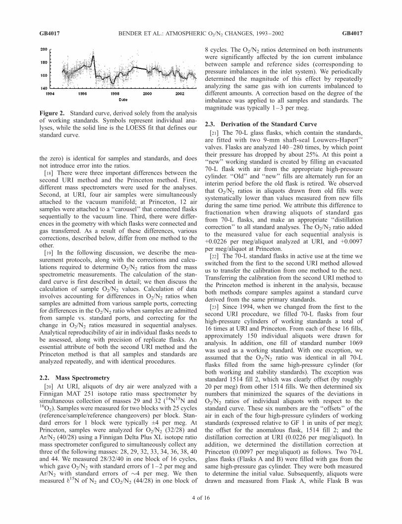
the zero) is identical for samples and standards, and doesnot introduce error into the ratios.[18] There were three important differences between the

second URI method and the Princeton method. First,different mass spectrometers were used for the analyses.Second, at URI, four air samples were simultaneouslyattached to the vacuum manifold; at Princeton, 12 airsamples were attached to a ‘‘carousel’’ that connected flaskssequentially to the vacuum line. Third, there were differ-ences in the geometry with which flasks were connected andgas transferred. As a result of these differences, variouscorrections, described below, differ from one method to theother.[19] In the following discussion, we describe the mea-

surement protocols, along with the corrections and calcu-lations required to determine O2/N2 ratios from the massspectrometric measurements. The calculation of the stan-dard curve is first described in detail; we then discuss thecalculation of sample O2/N2 values. Calculation of datainvolves accounting for differences in O2/N2 ratios whensamples are admitted from various sample ports, correctingfor differences in the O2/N2 ratio when samples are admittedfrom sample vs. standard ports, and correcting for thechange in O2/N2 ratios measured in sequential analyses.Analytical reproducibility of air in individual flasks needs tobe assessed, along with precision of replicate flasks. Anessential attribute of both the second URI method and thePrinceton method is that all samples and standards areanalyzed repeatedly, and with identical procedures.

2.2. Mass Spectrometry

[20] At URI, aliquots of dry air were analyzed with aFinnigan MAT 251 isotope ratio mass spectrometer bysimultaneous collection of masses 29 and 32 (14N15N and16O2). Samples were measured for two blocks with 25 cycles(reference/sample/reference changeovers) per block. Stan-dard errors for 1 block were typically ±4 per meg. AtPrinceton, samples were analyzed for O2/N2 (32/28) andAr/N2 (40/28) using a Finnigan Delta Plus XL isotope ratiomass spectrometer configured to simultaneously collect anythree of the following masses: 28, 29, 32, 33, 34, 36, 38, 40and 44. We measured 28/32/40 in one block of 16 cycles,which gave O2/N2 with standard errors of 1–2 per meg andAr/N2 with standard errors of �4 per meg. We thenmeasured d15N of N2 and CO2/N2 (44/28) in one block of

8 cycles. The O2/N2 ratios determined on both instrumentswere significantly affected by the ion current imbalancebetween sample and reference sides (corresponding topressure imbalances in the inlet system). We periodicallydetermined the magnitude of this effect by repeatedlyanalyzing the same gas with ion currents imbalanced todifferent amounts. A correction based on the degree of theimbalance was applied to all samples and standards. Themagnitude was typically 1–3 per meg.

2.3. Derivation of the Standard Curve

[21] The 70-L glass flasks, which contain the standards,are fitted with two 9-mm shaft-seal Louwers-Hapert

TM

valves. Flasks are analyzed 140–280 times, by which pointtheir pressure has dropped by about 25%. At this point a‘‘new’’ working standard is created by filling an evacuated70-L flask with air from the appropriate high-pressurecylinder. ‘‘Old’’ and ‘‘new’’ fills are alternately run for aninterim period before the old flask is retired. We observedthat O2/N2 ratios in aliquots drawn from old fills weresystematically lower than values measured from new fillsduring the same time period. We attribute this difference tofractionation when drawing aliquots of standard gasfrom 70-L flasks, and make an appropriate ‘‘distillationcorrection’’ to all standard analyses. The O2/N2 ratio addedto the measured value for each sequential analysis is+0.0226 per meg/aliquot analyzed at URI, and +0.0097per meg/aliquot at Princeton.[22] The 70-L standard flasks in active use at the time we

switched from the first to the second URI method allowedus to transfer the calibration from one method to the next.Transferring the calibration from the second URI method tothe Princeton method is inherent in the analysis, becauseboth methods compare samples against a standard curvederived from the same primary standards.[23] Since 1994, when we changed from the first to the

second URI procedure, we filled 70-L flasks from fourhigh-pressure cylinders of working standards a total of16 times at URI and Princeton. From each of these 16 fills,approximately 150 individual aliquots were drawn foranalysis. In addition, one fill of standard number 1069was used as a working standard. With one exception, weassumed that the O2/N2 ratio was identical in all 70-Lflasks filled from the same high-pressure cylinder (forboth working and stability standards). The exception wasstandard 1514 fill 2, which was clearly offset (by roughly20 per meg) from other 1514 fills. We then determined sixnumbers that minimized the squares of the deviations inO2/N2 ratios of individual aliquots with respect to thestandard curve. These six numbers are the ‘‘offsets’’ of theair in each of the four high-pressure cylinders of workingstandards (expressed relative to GF 1 in units of per meg);the offset for the anomalous flask, 1514 fill 2; and thedistillation correction at URI (0.0226 per meg/aliquot). Inaddition, we determined the distillation correction atPrinceton (0.0097 per meg/aliquot) as follows. Two 70-Lglass flasks (Flasks A and B) were filled with gas from thesame high-pressure gas cylinder. They were both measuredto determine the initial value. Subsequently, aliquots weredrawn and measured from Flask A, while Flask B was

Figure 2. Standard curve, derived solely from the analysisof working standards. Symbols represent individual ana-lyses, while the solid line is the LOESS fit that defines ourstandard curve.


4 of 16

GB4017

stored. After Flask Awas analyzed approximately 160 times,both flasks were analyzed to determine the distillation.[24] One needs to address questions of diffusion of gases

through O-rings for standards as well as samples. The largeamount of gas suppresses the effects of diffusion. On thebasis of our tests as well as those of Sturm et al. [2004],diffusion would change the O2/N2 ratios of the standards inthe 70-L glass flasks by <1 per meg/yr under normal usage.However, the change was much greater in our earlieststandards, which were highly depleted and stored for manyyears. Accordingly, analyses of these standards wererejected after approximately 5 years of storage.[25] The final step in constructing the standard curve

involved deriving the difference between O2/N2 ratios ofstandard fills analyzed at URI against the URI reference gas,and the standard fills analyzed at Princeton against thePrinceton reference gas. We determined the Princeton-URIdifference in three ways. First, we calculated the meanPrinceton–URI difference of all aliquots from the nine70-L flasks that were analyzed repeatedly at both institu-tions. The difference was �48 ± 5 per meg (1s, n = 9common 70-L flasks); the sign indicates that relative to thereference gas, the numbers at URI were higher than thenumbers at Princeton. Second, we limited this comparisonto aliquots analyzed during the final 5 months that the URIlab was active, and the first 5 months that the Princeton labwas active. The Princeton-URI difference was then �44 ±3 per meg (1s, n = 9 flasks). Finally, we calculated averageO2/N2 ratios for all aliquots filled from a given high-pressure cylinder at Princeton, and compared these numberswith comparable averages for standards analyzed at URI.The mean difference between the averages for flasks filledat Princeton from those at URI was �42 ± 2 per meg. Forconstructing the standard curve, we adopt a value of�48 per meg, the result of the largest data set. This numberprovides continuity between URI and Princeton, but it doesnot enter into the calculation of sample O2/N2 values. Thesedepend only on the difference in O2/N2 ratios of samplesfrom standards measured contemporaneously against thesame reference gas.[26] The entire standard curve is shown in Figure 2. The

points represent individual aliquots, and the line representsthe standard curve as derived using LOESS [Cleveland andDevlin, 1988]. Fitting terms for LOESS were f = 0.2, N = 5,d = 0. The key term is f, which determines the extent ofsmoothing. We chose a value of 0.2, which corresponds tosmoothing over about 70 individual standard analyses, andis a good compromise between using a large number ofstandard data for computing sample ratios, and a shortenough interval to capture variability in the standard curve.The standard deviation of individual aliquots from the curveis ±7 per meg for URI the period, and ±4 per meg for thePrinceton period. The reader will note that the standardcurve sometimes shows rapid variations where it may bemore uncertain. In general, however, few samples wereanalyzed at times when the standard curve was unstable.The sharp excursion in the second half of 1996 was notassociated with any change in analytical methods.[27] The derivation of the standard curve assumes that all

fills from a given high-pressure cylinder start with the same

O2/N2 ratio. In practice, we recognize that there is somevariability: standard flasks are not filled perfectly reproduc-ibly. We can assess this variability as follows. The standardcurve is determined by fitting data from all workingstandard flasks that are active. Typically, there are fiveactive flasks, one for each working standard cylinder, anda flask containing a prior fill that has not yet been retired.Hence each standard fill makes a small contribution (�20%)to the contemporaneous part of the standard curve. Wecalculated the mean deviation for each of our 18 workingstandard fills (excluding the single fill of 1069 used as aworking standard, and 1514f2). The standard deviation ofthe mean of a single fill from all fills from the same high-pressure cylinder is 1.4 per meg (n = 15 fills). This numberprovides a measure of variability in initial O2/N2 of 70-Lflasks filled from a given standard cylinder. The worst casewas 2706 fill 2, which differed from the mean offset of fillsfor tank 2706 by 4 per meg. At any one time, the standardcurve is calculated by averaging O2/N2 ratios from four ormore flasks, and the standard error in the standard curve dueto errors in filling 70-L flasks is thus less than 1 per meg.[28] O2/N2 ratios of stability standards are corrected for

distillation and then calculated by subtracting the standardcurve from the measured values. If the standard curve trulycaptures the drift in the analysis system, the O2/N2 ratios ofindividual stability standards calculated in this mannershould be constant over time. One measure of accuracy inthe standard curve comes from the variability in O2/N2

ratios measured in individual stability standards. For theentire Princeton analysis period (to the first quarter of 2005)the standard deviation from the mean for a given fillranges from ±3.2 per meg to ±5.9 per meg, with one outlier,which has been analyzed only a small number of times, at±7.1 per meg. These numbers are based on 1212 individualanalyses of 11 fills, with 28 highly anomalous resultsexcluded from the calculations. We also tested for longterm drift in the standard curve by subtracting the meanfrom the O2/N2 ratios measured for individual aliquots, andplotting the mean versus time. Because the actual O2/N2

ratio of the individual stability standard fills is constant withtime, any trend in the residuals reflects drift in the standardcurve. The slopes of best-fit lines correspond to standardcurve drifts of �0.23 ± 0.24 (s. e.) per meg yr�1. This ratecorresponds to an error of 0.1 ± 0.1 Gt C yr�1 in partitioningCO2 sequestration between land and ocean.

2.4. Methods of Sample Analysis

[29] The second URI method, and the Princeton methodthat followed, were designed to allow analysis of 500–1000or more sample flasks per year, with extensive standardiza-tion and high precision. To achieve these goals, the methodshad the following attributes: automated analyses undercomputer control using LabVIEW

TM

, the presence of multi-ple equivalent ports for admitting samples, expansion ofsamples and reference gases at 1 atm nominal pressure tominimize fractionation, identical processing procedure forall samples, identical processing procedure (to the extentpossible) for admitting standards and samples, use of inertvacuum line materials wherever possible, and high precisionas a result of long analysis times.


5 of 16

GB4017

[30] Both procedures were set up so that samples andreference gases were analyzed in an automated sequencelasting 14–18 hours that was started in the afternoon andcompleted early the following morning. Daytime was re-served for replicate analyses of flasks, additional standardanalyses, maintenance, etc.2.4.1. Second URI Method[31] The glass vacuum line for the second URI method

is shown in Figure 3. It included ports for two 70-Lstandard flasks and four 2-L sample flasks, and valvesleading to the pumps and the variable volume. The gas inthe 70-L ‘‘daily standard flask’’ was analyzed frequently asa guide to instrumental stability, but was not used forconstraining the standard curve. In a normal run, a 70-Lstandard flask and four sample flasks were attached to themanifold. After evacuation, manual valves of these fiveflasks were opened, allowing the gas to expand to theautomated glass valves of the manifold that then isolatedeach port. A sample or standard was expanded through theline into the variable volume. At this point it began

flowing through the capillary tube to the sample side ofthe mass spectrometer’s changeover valve. A glass valvewas closed to isolate the variable volume, which was aglass cylinder with a moveable aluminum piston sealed bytwo O-rings. This volume was adjusted by moving thepiston with a stepper motor to balance ion currents onsample and reference sides. The sample was then analyzedfor O2/N2 in two blocks, 25 cycles/block. The line wasevacuated and the sample was reanalyzed using theidentical procedure. Then the next sample or standardwas admitted, and so on. The standard was analyzed3 times in each nightly cycle: before the first sample,before the third sample, and after the fourth sample.[32] Each measured O2/N2 ratio was corrected for the

pressure imbalance between sample and reference sides asdescribed earlier. The O2/N2 ratios of aliquots after the firstwere corrected for the (small) change in O2/N2 compositionas air was drawn from the flask; the correction was of order1 per meg/aliquot. Samples were analyzed on differentports; in general, no systematic difference in O2/N2 ratio

Figure 3. Schematic of the inlet line used at U. R. I. used in the second U. R. I. method.


6 of 16

GB4017

could be detected. At one point, a dirt particle lodged on theO-ring of one of the four automated glass valves used toadmit aliquots from a sample flask, causing the O2/N2 ofthis port to be in error, initially by 5.1 ± 0.9 (s.e.) per meg,and later by 9.4 ± 1.5 (s.e.) per meg. We did not change thisO-ring as it would have meant disassembling delicate partsof the apparatus. Rather, the appropriate correction wasapplied.[33] Air admitted from the standard port expands into

the vacuum manifold in a way that is different from airadmitted at the sample ports. To evaluate the possibilitythat gas introduced on the standard port is fractionateddifferently from gas introduced at the sample ports, weadmitted samples from the same bottle on both ports. Thisexperiment was carried out with 5-L flasks of the typeused by R. Keeling [Keeling et al., 1998]; these largeflasks allowed the analysis of multiple aliquots on bothports. Samples admitted on the sample port had O2/N2 =8.5 ± 0.8 (standard error) per meg higher than those on thestandard port. Thus we subtracted 8.5 per meg from allsample values to make sample and reference gases fullycomparable.[34] The standard deviation from the mean O2/N2

ratios measured in sequential blocks (of 25 cycles) fromthe same inlet is ±6.7 per meg (1s, n = 12,996). In thisand some of the following cases, deviations were notnormally distributed. We report both the standard devi-ation and also the deviation from the mean encompass-ing 68% of the data points (corresponding to 1 sigmafor normally distributed errors). Sixty-eight percent ofblocks have a deviation from the mean �3.1 per meg.The standard deviation from the mean of O2/N2 ratiosdetermined with replicate sample inlets (can be up tonine inlets) is ±5.9 per meg (1s). Sixty-eight percent ofreplicate inlets have O2/N2 ratios that deviate from themean by �2.7 per meg.[35] O2/N2 ratios for replicate flasks are excluded

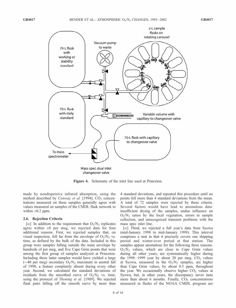
from the concentration record when the flasks differ by>16 per meg. 91 out of 1143 pairs are excluded by thiscriterion. The standard deviation from the mean ofretained values is ±3.1 per meg. Following Keeling etal. [1998], we calculate scaled residuals (di) according totheir equation (5), multiplying deviations from the meanby (N/(N�1))0.5, where N represents the number ofreplicates. Flasks were measured in duplicate, and thescaled residuals are thus ±4.4 per meg.2.4.2. Princeton Method[36] The Princeton inlet system (Figure 4) differs from the

URI inlet system primarily in the way samples areconnected to the inlet line. The Princeton inlet includes aglass manifold with Louwers-Hapert

TM

valves to vacuum,variable volume, primary or stability standards, workingstandard, and carousel. The carousel is a translating androtating ring to which 12 samples can be connected. In theretracted position, the carousel can be rotated so that a flaskof choice will, when engaged, mate to the manifold. In theengaged position, the flask is connected to the vacuummanifold by an aluminum transfer tube, and the flask valvehandle is connected by a drive shaft to a rotating cog drivenby a stepper motor. The latter allows the flask valve to be

opened or closed under computer control. One end of thealuminum transfer tube is sealed to the outlet valve of thesample flask with a compression fitting and Viton

TM

O-ring.The other end has a polished aluminum face, which sealsagainst a Viton

TM

quad-ring of the vacuum manifold at 30 psiforce.[37] The carousel inlet has three major advantages. First,

every sample enters the vacuum manifold in the samegeometry. Second, each sample sees the minimum amountof vacuum components (no tubing or O-rings are used toattach and isolate other flasks to a common manifold).Third, the compact geometry reduces thermal gradients inthe system, and all gas flow occurs in a horizontal plane,eliminating significant gravitational fractionation.[38] The protocol for sample analysis is as follows. Twelve

samples and a working or stability standard are put in placeand allowed to passively reach temperature equilibrium for1–3 hours. Then each sample is in turn admitted to themass spectrometer and analyzed, as described earlier, forN2/O2/Ar (28/32/40) and N2/

15N14N/CO2 (28/29/44). Thenthree aliquots of the standard are admitted and analyzed inthe identical manner. The next day, a new standard and thesame samples are analyzed, each sample being shiftedforward by 1 port position on the carousel. Approximatelya week later, the replicate flasks are analyzed in theidentical manner. They are placed on the carousel in thesame sequence but the port positions are shifted by 4 fromthe initial positions.[39] A subset of samples is measured on the standard port

so that a correction can be made, as in the URI method, forrelating O2/N2 ratios of samples to standards. During theanalysis period for samples reported here, 761 samples wereanalyzed on the standard port as well as the sample ports.The sample port–standard port difference, averaged overanalysis intervals, ranged from 2 to 22 per meg, with valuesover 14 pertaining to only a small fraction of the analysisperiod when mass spec stability was poor. Samples arecorrected with the appropriate difference given their analy-sis date.[40] The analysis protocol gives extensive information

about sample port-to-sample port differences in measuredO2/N2 ratios. External precision, based on a representativesubset of replicate analyses of samples from the sameflask and carousel port, is ±4.3 per meg (1s, n = 1296).Sixty-eight percent of replicate analyses lie within2.8 per meg of the mean. Systematic port-to-port differ-ences in O2/N2 for the same flask are up to 2 per meg.No corrections were made for these differences, whichtend to cancel given that flasks and their replicates areanalyzed on different ports. Data from 64 out of 731 pairsof flasks were rejected from the six sites reported on inthis paper because flask means differed by >16 per meg.Precision (standard deviation from the mean) for remain-ing replicate flasks was ±3.3 per meg. Again the flaskswere measured in duplicate, and the scaled deviation is±4.7 per meg.

2.5. CO2 Measurements

[41] After O2/N2 analysis, the flasks were sent to NOAA/CMDL for CO2 measurements. The measurements were


7 of 16

GB4017

made by nondispersive infrared absorption, using themethod described by Conway et al. [1994]. CO2 concen-trations measured on these samples generally agree withvalues measured on samples of the CMDL flask network towithin ±0.2 ppm.

2.6. Rejection Criteria

[42] In addition to the requirement that O2/N2 replicatesagree within ±8 per meg, we rejected data for fouradditional reasons. First, we rejected samples that, onvisual inspection, fell far from the envelope of O2/N2 vs.time, as defined by the bulk of the data. Included in thisgroup were samples falling outside the main envelope byhundreds of per meg, and five Cape Grim points that wereamong the first group of samples analyzed at Princeton.Including these latter samples would have yielded a large(�40 per meg) secondary O2/N2 maximum in austral fallof 1998, a feature completely absent during every otheryear. Second, we calculated the standard deviations ofresiduals from the smoothed curve of O2/N2 vs. time,using the protocol of Thoning et al. [1989]. We rejectedflask pairs falling off the smooth curve by more than

4 standard deviations, and repeated this procedure until nopoints fell more than 4 standard deviations from the mean.A total of 72 samples were rejected by these criteria.Several factors would have lead to anomalous data:insufficient drying of the samples, undue influence onO2/N2 ratios by the local vegetation, errors in samplecollection, and unrecognized transient problems with themass spec inlet line.[43] Third, we rejected a full year’s data from Syowa

(mid-January 1998 to mid-January 1999). This intervalcomprises a unit in that it precisely covers one shippingperiod and winter-over period at that station. Thesamples appear anomalous for the following three reasons.O2/N2 values, which are close to Cape Grim valuesduring all other years, are systematically higher duringthe 1998–1999 year by about 20 per meg. CO2 valuesat Syowa, measured in the O2/N2 samples, are higherthan Cape Grim values, by about 0.5 ppm, throughoutthe year. We occasionally observe higher CO2 values atSyowa, but, in other years, the discrepancy never lastsmore than about 6 months. Finally, CO2 concentrationsmeasured in flasks of the NOAA CMDL program are

Figure 4. Schematic of the inlet line used at Princeton.


8 of 16

GB4017

anomalously high, and anomalously noisy, during this period(ftp.cmdl.noaa.gov).[44] Finally, certain CO2 data are rejected according to

criteria of Conway et al. [1994].

3. Results

[45] O2/N2 and CO2 measured at our six sampling stationsare shown in Figure 5. The data show the expected trends[e.g., Keeling and Shertz, 1992; Keeling et al., 1998; Battleet al., 2000]: CO2 concentrations increase with time, whileO2/N2 ratios decrease. The seasonal cycles of O2/N2 andCO2 are out of phase. The amplitude of O2/N2 cycles islarger than that of CO2: amplitudes due to land sources arecomparable, but the seasonal source of the ocean is muchgreater for O2 than for CO2.

3.1. Equations for Calculating Land and OceanCarbon Sequestration

[46] Data from Barrow, Cape Grim, and Samoa areused to partition anthropogenic CO2 uptake by the landbiosphere and the ocean. These sites have the longestrecords, greatest sampling frequency (weekly over muchof the records), and fewest gaps. Sampling began inspring 1991 at Cape Grim; in February 1993 at Barrow;and in June 1993 at Samoa. Hence, in order to havecomplete data sets, we restrict the calculation of landand ocean carbon uptake to the period from 1994 to2002.

[47] Global CO2 concentrations and O2/N2 ratios werecalculated by simple averaging of values at Barrow, Samoa,and Cape Grim,

CO2ð Þglobal¼ CO2ð ÞBRW þ CO2ð ÞCGT þ CO2ð ÞSMO

� �=3 ð2Þ

d O2=N2ð Þglobal¼ d O2=N2ð ÞBRW þ d O2=N2ð ÞCGT þ d O2=N2ð ÞSMO

� �=3

ð3Þ

[48] For our purposes, it is important that these valuesaccurately reflect annual changes in the gas properties,rather than that they give accurate measures of the globalaverage at any one time.[49] The atmospheric mass balance of CO2 and O2 are

expressed as follows [Battle et al., 2000]:

dðCO2Þdt

¼ �b� ffuel þ fcement þ fland þ foceanð Þ ð4Þ

d O2=N2ð Þdt

¼ g� b� afuel ffuel þ abiofland� �

: ð5Þ

Units of CO2 are ppm, O2/N2 are per meg, and f (flux)terms are Gt C yr�1. Here a is dimensionless, b has unitsof ppm/Gt, and g of per meg/ppm. All flux terms arenegative for flux to the atmosphere (i.e., positive fluxes

Figure 5. O2/N2 and CO2 records of this study.


9 of 16

GB4017

correspond to net CO2 uptake by the oceans and the landbiosphere). The ffuel and fcement are sources of CO2 fromfossil fuel burning and cement manufacturing, respectively.The focean and fland are the ocean and terrestrial biospheresinks of CO2. afuel is the average O2:C molar exchangeratio for fossil fuels burned during the period of O2 andCO2 measurement, and abio is the O2:C molar exchangeratio for photosynthesis and respiration. The b converts GtC to ppm CO2, and g converts ppm to per meg. Values forb, g, abio, and afuel are summarized in Table 3. Equations(4) and (5) assume that the annually averaged O2

inventory of the oceans is constant. In fact, there is strongevidence that this inventory has been decreasing, with anassociated flux of O2 from ocean to atmosphere. We firstcalculate sequestration neglecting this change, then makean appropriate correction for the changing ocean O2

inventory.[50] O2 consumed by fossil fuel burning is calculated

from fossil fuel combustion estimates of Marland et al.[2003], assuming that utilization of all sources rose by 1%in 2001 and 2002 (years for which data are not yetavailable); afuel was determined from the utilization-weighted average DO2/DCO2 for natural gas (�1.95),crude oil (�1.44), solid carbon (�1.17), and gas flaring(1.98) [Keeling, 1988]. For the total fossil fuel combustedfrom 1994–2002, aF was �1.45. Solving equations (4)and (5) for fland and focean in terms of measured and knownquantities, we obtain

fland ¼ �afuel

abio

ffuel þ1

bgabio

d O2=N2ð Þdt

ð6Þ

focean ¼� abio � afuel

abio

ffuel � fcement �d CO2ð Þ=dt

b

� 1

bgabio

d O2=N2ð Þdt

: ð7Þ

[51] Atmospheric potential oxygen, APO, which isunaffected by exchange of CO2 and O2 between theatmosphere and the land biosphere [Stephens et al.,1998], is defined as

APO ¼ O2=N2 þ gabioCO2: ð8Þ

Hence, after combining and rearranging equations (4), (5)and (8), we obtain

dAPO

dt¼ g� b� abio

afuel � abio

� �abio

ffuel � fcement � focean

� �: ð9Þ

Solving equation (9) for focean in terms of measured orknown quantities, we obtain

focean ¼ �abio � afuel

abio

ffuel � fcement �1

bgabio

d APOð Þdt

: ð10Þ

Then

fland ¼ �ffuel � fcement � focean �1

bdCO2

dt: ð11Þ

3.2. Partitioning of CO2 Sequestration, 1994–2002

[52] Our observations begin in 1991 at Cape Grim and in1993 at Samoa and Barrow. We base our calculation ofsequestration on these three sites because, elsewhere, obser-vations commence more recently and sampling density islower. We make calculations for the period mid-1993 tomid-2002 based on data from Cape Grim only, and betweenmid-1994 and mid-2002 based on data from Cape Grim,Samoa, and Barrow. We emphasize that the products ofthese calculations are net global fluxes of CO2 between theland biosphere and the atmosphere, or between the oceansand the atmosphere.[53] Between mid-1993 and mid-2002, 56.3 Gt C was

released to the atmosphere from fossil fuel combustion andanother 1.9 from cement manufacture [Marland et al.,2003]. At the same time, the atmospheric CO2 concentra-tion, as represented by data from CGO, rose by 15.3 ppm(32.5 Gt C). Therefore the total carbon sink averaged2.9 Gt C yr�1 over the study period. Ocean and land uptakerates calculated from our data are 1.8 and 1.1 Gt C yr�1,respectively. From mid-1994 to mid-2002, we can make thiscalculation by averaging data from Barrow, Cape Grim,and Samoa. For this period, ocean and land CO2 uptakeaverage 1.4 and 1.3 Gt C yr�1, respectively. (Correctedfor ocean O2 outgassing, as explained below, we calcu-late ocean and land CO2 sequestration rates, respectively,as 2.1 and 0.8 Gt C yr�1 from 1993–2002, and 1.7 and1.0 Gt C yr�1 from 1994–2002.)[54] In making these estimates, we calculate CO2 and

APO values for individual flask samples using equation (8).We then calculate deseasonalized CO2 and APO values forBRW, SMO and CGO, with 620-day smoothing, using thealgorithm of Thoning et al. [1989] (hereinafter referred to asCCGVu). This level of smoothing is roughly equivalent to a1-year running average. From these curves, we calculateannually averaged values at BRW, SMO, and CGO, and, for1994–2002, calculate the yearly global average of the threesites. Using these values, we calculate sequestration ratesfrom equations (10) and (11). Fossil fuel combustion ratescome from Marland et al. [2003]; other terms are summa-rized in Table 3.[55] These numbers need to be modified to account for

the transfer of O2 from ocean to atmosphere, and it is to thissubject that we turn next. Global warming is likely to lead tosome transfer of O2 from the ocean to the atmosphere. Sucha change would lead to an increase in the atmospheric O2

inventory, which we would incorrectly attribute to a carbonflux to the land biosphere. The possibility of an ocean efflux

Table 3. Conversion Factors and Other Terms for Calculating the

Anthropogenic Mass Balance

Symbol Description Number

b Gt C to ppm CO2 0.471g ppm O2 to per meg d(O2/N2) 4.8afuel mean DO2/DCO2 during combustion �1.45abio mean DO2/DCO2 during photosynthesis/respiration �1.1


10 of 16

GB4017

arises for two basic reasons. First, the ocean is warming,lowering solubilities and causing degassing. Since O2 ismore soluble than N2, the O2/N2 ratio of air rises. The ratemay be estimated from the increased heat load of the oceans[Levitus et al., 2000], although one also needs to estimatethe temperature distribution of the warming waters.[56] Second, the ocean carbon cycle may be changing in a

way that induces transfer of O2 to the atmosphere. Increasedupper ocean stratification, expected given upper oceanwarming and high-latitude freshening, will lead to increasedutilization of nutrients. This change, in turn, increases theexport of organic carbon to depth; it decreases the fractionof ‘‘preformed’’ nutrients that go unutilized in surface waterand passively sink during subduction [e.g., Keeling andGarcia, 2002]. Furthermore, an increase in the C/nutrientratio of organic matter in oligotrophic waters would induceO2 transfer to the atmosphere. Such a change has beeninvoked to explain decreasing [O2] in the upper thermoclineof the subtropical North Pacific [Emerson et al., 2001].[57] A considerable effort has gone into assessing the rate

of ocean O2 degassing. We may divide the work into threeapproaches: local, large-scale and model studies. First, incareful local studies, Emerson et al. [2001] document alarge decrease in dissolved O2 in thermocline waters from25�–45� N along a meridional line through the subtropicalNorth Pacific gyre (described above), and Shaffer et al.[2000] find decreasing [O2] in waters off the Chilean coast.Andreev and Watanabe [2002] conclude that [O2] is risingin waters of the subpolar North Pacific; however, the trendmay disappear if one removes the decadal cyclicity that theauthors link to the North Pacific Index. Second, three large-scale (basin-wide or global) studies demonstrate littlechange in O2 inventories during recent decades, and noevidence for systematic decreases in ocean [O2] [Pahlowand Riebesell, 2000; Bindoff and McDougall, 2000; Kelleret al., 2002]. On the other hand, Matear et al. [2000]analyzed a limited data set and deduced significant O2

outgassing in a 30� zonal sector of the Southern Ocean.This result agrees with their model predictions of increasedSouthern Ocean stratification, diminished ventilation, andhence decreasing dissolved [O2] in seawater. Third, threeadditional modeling studies [Sarmiento et al., 1998;Plattner et al., 2002; Bopp et al., 2002] and a data analysispaper [Keeling and Garcia, 2002] estimate the rate of O2

outgassing by empiricism and deduction. Each estimates anO2 flux to the atmosphere of 5–6 nmol O2/Joule of oceanwarming (mainly due to a changing carbon cycle), andcalculates the recent O2 efflux from the heat flux ofLevitus et al. [2000]. Their calculated O2 fluxes differ bya factor of 2 (corresponding to a sequestration correction of0.3–0.6 Gt C yr�1) due largely to differences in adoptedvalues of the heat flux.[58] We have adopted the lower estimates (0.3 Gt C yr�1)

for four reasons. First, existing basin-scale studies do notsupport large outgassing except in the Southern Ocean,where few data have been analyzed. Second, biogeochem-ical outgassing is likely to be small during the early part ofthe anthropogenic transient, because much of the heatstorage is in the upper water column [Levitus et al.,2000]. Since these waters are largely nutrient-free (O2* �

[O2]sat) in the analysis of Keeling and Garcia [2002],warming cannot induce much increase in net euphotic zonenutrient utilization and biogeochemical O2 outgassing.Third, most whole-ocean warming from 1990–1995 takesplace in the first year and a half of the decade [Levitus et al.,2000]. This 1.5- year period, included in the Bopp analysis,predates our study period. Finally, Keeling and Garcia basedtheir estimate of ocean warming on the heat content recordof the upper 300 m, which extends to 1998. Throughextrapolation, they account for warming below 300 m(climatologically about 25% of the total), and their correc-tion is more appropriate to our record.[59] Ultimately, the current uncertainty in the O2 outgas-

sing correction is less important than the ability of thecommunity to narrow the uncertainty in the coming years.Current O2-based estimates of land and ocean carbon se-questration have an uncertainty of order ±0.3 Gt C yr�1yr�1

due to uncertainty about the rate of ocean outgassing. Weexpect that the uncertainty will be narrowed by theanalysis of historical ocean O2 concentration data, supple-mented by the ongoing CLIVAR Repeat HydrographyProgram, and by studies with models carefully evaluatedin the context of these extensive data sets.[60] Invoking the correction of 0.3 Gt C yr�1 raises

calculated ocean uptake for 1993–2002 to 2.1 Gt C yr�1

and lowers land uptake to 0.8. For the 1994–2002 period,the comparable numbers are 1.7 and 1.0 Gt C yr�1,respectively. If one used the modeled corrections of0.60 Gt C yr�1, one would estimate ocean uptake at 2.0–2.4 Gt C yr�1 (starting in 1993 and 1994, respectively), andnet land uptake as 0.5–0.7 Gt C yr�1. The latter result stillimplies a large land sink, since terrestrial deforestation givesregional sources that sum to order 1 Gt C yr�1 [Schimel etal., 2001].[61] Uncertainties in these numbers arise from analytical

errors, uncertainties in the change in atmospheric O2 andCO2 due to limited sampling, uncertainties in air-sea O2

exchange, and uncertainties in fossil fuel combustion ratesand stoichiometry. We consider that the analytical errorsare negligible with respect to calculations of carbonsequestration over the length of the record, because ofthe absence of detectable drift in stability standards and thelarge number of samples analyzed. For reference, O2/N2

drift of 0.5 per meg/year (2 s of the stability standarddrift) corresponds to an error in carbon partitioning of0.2 Gt C yr�1 in the land and ocean reservoirs. Weestimate the error in sampling the atmosphere from thesites having the poorest agreement in APO changes from1994–2002. These are Barrow and Cape Grim, whichdiffer by ±3 per meg over the length of the record. Thisdifference translates to an uncertainty in partitioning ofabout 0.1 Gt C yr�1. We estimate the uncertainty incombustion rate as ±0.4 Gt C yr�1 [Keeling and Shertz,1992]; this term leads to an uncertainty in ocean uptake of±0.1 Gt C yr�1, and land C uptake of ±0.4 Gt C yr�1.(Equation (10) shows that uncertainty due to combustionis smaller for ocean sequestration because it enters onlyas the difference between land biosphere and fossil fuelstoichiometry.) Finally, we estimate the uncertainty inabio as ± 0.05 (estimated from results of Severinghaus


11 of 16

GB4017

[1995]). The corresponding uncertainty in partitioning is±0.3 Gt C yr�1. To these numbers, we must add anadditional uncertainty of ±0.3 Gt C yr�1 due to the oceanO2 imbalance. It is difficult to know how to propagatethese uncertainties. We recognize that they are not nor-mally distributed but nevertheless choose to add themquadratically, since they are independent, and unlikely toall trend in the same direction. The resulting uncertainty is±0.5 Gt C yr�1 for ocean sequestration and ±0.6 Gt C yr�1

for land sequestration.[62] Our computed carbon sequestration rates are com-

pared with other recent estimates of ocean uptake in Table 4.With respect to ocean uptake, O2/N2 based studies such asours access rates of fossil fuel CO2 uptake by the oceans,whereas studies of air-sea pCO2 disequilibrium and atmo-spheric inversions access net oceanic CO2 uptake. Thenumbers differ by the amount of ocean degassing due tooxidation in the oceans of terrestrial organic matter, andprecipitation of CaCO3 [Sarmiento and Sundquist, 1992].These two fluxes sum to 0.6 Gt C yr�1, and we correct?pCO2 and inversion flux estimates for these terms. Tabu-lated rates of fossil fuel CO2 uptake by the ocean (takinginversion estimates as a single number) then fall within therange 2.2 ± 0.6 Gt C yr�1. Some variability may be due tothe fact that different approaches characterize differenttimes; we cannot now say. Estimates based on O2/N2 datacontinue to be near the lower end of the range.

3.3. Interannual Variability in Land andOcean CO2 Uptake

[63] Equations (10) and (11) show how calculated valuesof focean and fland depend on fossil CO2 sources, stoichio-metric terms, and rates of change of O2/N2, CO2, and APO.Over the length of the O2/N2 record, fossil terms andstoichiometric terms change slowly, and calculated ratesof sequestration change mainly because of variations inrates of change of O2/N2 and APO (Figure 6). Land CO2

sequestration can be calculated from the rate of change ofO2/N2 alone (equation (6)), and decreases as d(O2/N2)/dtbecomes more negative. Ocean CO2 sequestration can becalculated from the rate of change of APO alone (equation(10)), and increases as d(APO)/dt becomes more negative.(We note that these calculations can be made either by usingvalues of APO versus time calculated by CCGVu, as is done

here, or by adding values of O2/N2 and CO2 calculated byCCGVu. The results are not perfectly equivalent because ofdetails of the curve fits. Differences in ocean sequestrationcalculated by the two methods are far smaller than thevariation of the rates calculated from fitting APO vs. time,and are not considered further.)[64] We calculate rates of change in O2/N2 and APO from

the trend in deseasonalized values fitted to observationsusing the CCGVu program [Thoning et al., 1989] with a620-day smoothing period, corresponding roughly to 1-yearsmoothing. As one estimate of the analytical error, weanalyze data for the period from 999 to 2005 from threestability standards (1069, 1510, and 2619) in the same way

Table 4. Oceanic CO2 Uptake During the 1990s Calculated in This Study and Other Recent Worka

Method Period Ocean Net Ocean Fossil

O2/N2 (CGO only: this paper) 1993–2002 2.1 ± 0.5O2/N2 (BRW, CGO, SMO: this paper) 1994–2002 1.7 ± 0.5O2/N2 (Manning [2001]) 1990–2000 1.7 ± 0.5Sea surface pCO2 (Takahashi et al. [2002]) 1995 2.2 ± 0.2 2.8Atmospheric CO2 inversion (Gurney et al. [2003]) 1992–1996 1.5 ± 1.1 2.1Atmospheric CO2 inversion (Rodenbeck et al. [2003]) 1990–1999 1.4 ± 0.3 2.0Ocean CO2 inventory (McNeil et al. [2003]) 1990s ��2.0 ± 0.4Ocean GCMs (13 models; McNeil et al. [2003]) 1990s 2.2–2.8

aUnits are Gt C yr�1. Values are reported as ocean net CO2 uptake and ocean uptake of fossil fuel CO2. Fossil uptake is greaterthan net uptake by 0.6 Gt C yr�1 owing to oxidation of riverine organic CO2 followed by CO2 outgassing, as well as byprecipitation of CaCO3, also followed by CO2 outgassing [Sarmiento and Sundquist, 1992; Ludwig and Probst, 1996]. Estimatesbased on O2/N2 ratios, from Manning [2001] (based on measurements in the laboratory of R. F. Keeling) and from this study,include an ocean outgassing correction of 0.3 Gt C yr�1. The constrained values are shown in bold print, and derived values inplain print.

Figure 6. Rates of change of O2/N2 (top) and APO(bottom) in smoothed deseasonalized records from our studysites. See color version of this figure at back of this issue.


12 of 16

GB4017

as our samples. The largest rate of inferred O2/N2 variabilityis about 1 per meg yr�1, corresponding to an error in land orocean sequestration of about 0.4 per meg yr�1.[65] In examining the O2/N2 and APO records, we divide

our sites into two groups. Cape Grim, Barrow, and Samoa,are our best constrained sites, with the longest records,fewest gaps, and highest sampling resolution (nominallyweekly). We focus primarily on these three sites. Fluxesderived from the observations at Amsterdam, Macquarieand Syowa are less well constrained, because records areshorter, gaps are present, and collection frequency is lower.[66] The pattern of O2/N2 variations is similar at each of

the three primary sites, and the amplitude of the variations iscoherent. These attributes give us confidence that thevariability does not originate with artifacts of sampling,which would cause each site to vary independently. Inprinciple, the variability could be analytical: samples fromthese sites collected at the same time were analyzed at aboutthe same time. However this source would require drift inthe standard curve of 5–10 per meg/year, sustained over aperiod of a year or so. Such drift is unlikely given theabsence of detectable drift in the stability standards, and theexcellent agreement of O2/N2 ratios measured for samplesanalyzed in our lab as well as the lab of R. Keeling[Manning, 2001]. Most of this variability is likely real. Asdiscussed below, it reflects the combined variations of CO2

uptake by the land biosphere, and interannual imbalances ofthe ocean O2 inventory.[67] The O2/N2 variations are highly correlated and

in phase between BRW and CGO. However, variationsat Samoa lead variations at the other two sites by upto 4 months (Figure 6). These results suggest that the landsequestration and ocean imbalance signals may originatemainly in the tropics. However, a firm conclusion ispremature, because the influences on O2/N2 at Samoaare complex [Manning et al., 2003], and because theSamoa lead is clearly absent for the latter part of therecord (Figure 6).[68] The variability in the rate of O2/N2 decrease at our

secondary sites is puzzling. The variations at SYO andMAC are larger than at our primary sites, and the excursionsare not coincident with those at the primary sites. Variationsat Syowa and Amsterdam coincide, and may represent anIndian Ocean signal. Our two closest sites, MAC and CGO,do not share much variability. MAC is at 55�S latitude, inthe middle of the Southern Ocean, and may be too stronglyaffected by local and synoptic scale variability to recordregional trends. A future paper will deal with interannualvariability at CGO, SYO, MAC, and AMS.[69] The amplitude of the APO variations is generally

smaller than those of O2/N2 (Figure 6). This characteristicreflects the fact that APO excludes variability in the landbiosphere. Unlike O2/N2 variations, APO variations are nothighly coherent at the major sites. In a lagged correlationanalysis, Barrow leads Cape Grim by about 0.5 years, andthe correlation coefficient is 0.57 at this phase (so that 34%of the filtered variance is shared). Shared variance is lowerbetween SMO and the other two sites. Nevertheless, weargue that there are strong similarities in the APO recordsfrom BRW, SMO, and CGO. Visual inspection of the record

shows that each of the three major sites has the samenumber of cycles between 1994 and 2002, although maximaand minima are offset by up to 6 months. As is the case withO2/N2, APO variability at the secondary sites is greater thanat the major sites, and variability is similar at Syowa andAmsterdam. Macquarie is distinct, and in fact variations indeseasonalized APO at Macquarie appear to be out of phasewith Cape Grim for much of the record.[70] If we assume all oceanic O2/N2 fluxes are tied to

carbon fluxes, we can use equation (10), together withcombustion rates and the atmospheric mass balance, tocompute variations in land and ocean fossil fuel CO2

sequestration rates since 1994. Such calculations do notcorrect for ocean O2 outgassing. Land and ocean seques-tration rates are plotted versus time in Figure 7, andcompared with total sequestration rates. The latter are con-strained by fossil fuel combustion rates and the atmosphericCO2 increase, both of which are well known. The mostcompelling result is that CO2 sequestration rates by the landbiosphere covary closely with total sequestration rates from1995–2001, except that the decrease in land sequestrationin 1999 leads total sequestration by about 6 months. Themost dramatic climate event during this period, the 1997–1998 El Nino, was accompanied by a rapid CO2 growthrate. Our data indicate that rapid CO2 growth was due to adiminished land sink (or small land source). This work thussupports many previous studies linking rapid atmosphericCO2 growth rates with diminished land carbon uptakeduring El Nino events [e.g., Keeling et al., 1989; Clark etal., 2003; Nemani et al., 2003; Schaefer et al., 2002;Reichenau and Esser, 2003]. The primary mechanism isnow thought to be increased aridity and biomass burning intropical areas during El Nino events [Langenfelds et al.,2002; van der Werf et al., 2004].[71] Another striking feature of the interannual variability

is its large magnitude in the oceans, and the anticorrelationof land and ocean variability during most of the record.During an El Nino event, both features are expected. OceanCO2 sequestration is enhanced because warming of theequatorial Pacific suppresses upwelling and the attendanttransfer of CO2 to the regional atmosphere [e.g., Feely et al.,2002]. At the same time, drying of tropical regions leads toa net CO2 flux from the land biosphere to the atmosphere(citations above).[72] Battle et al. [2000] used O2/N2 data (including data

presented here for BRW, CGO, and SMO) to estimate landand ocean CO2 sequestration between 1991 and 1998. Theycompared their results with sequestration rates inferred fromd13C of atmospheric CO2, which constrains these termsbecause land uptake discriminates strongly against theheavy isotope. Their data treatment differed from oursprimarily in that they smoothed with a filter equivalent toproducing a 2-year running average, whereas ours corre-sponds to 1 year. Their records of changing sequestrationrates were correspondingly smoother. For the period fromthe beginning of 1993 to mid-1996, their estimates ofvariations in land and ocean CO2 uptake based on O2/N2

closely tracked estimates based on d13C of CO2, a resultlikely to reflect real variability. The longer averaging timewill remove some artifacts associated with analytical errors


13 of 16

GB4017

and annual changes in air-sea O2 transfer, but here werestrict the comparison to 1-year smoothing.[73] At non El Nino times, the balance of evidence

suggests that the large ocean amplitude in sequestrationrates calculated with 1-year averaging (Figure 7), andocean-land antiphasing, are artifacts. They may resultfrom analytical error and/or non-zero net O2 exchangebetween the oceans and the atmosphere. During thesenon-El Nino times, there is no known coupling betweenthe oceans and land biosphere that would introduce out-of-phase behavior. Interpretations of the distribution ofCO2 in the atmosphere do not support out-of-phasebehavior. For example, Rodenbeck et al. [2003] used aninverse approach, together with atmospheric transportbased on reanalyzed winds, to calculate land and oceansequestration rates since 1982. They also summarizedearlier results of inverse calculations by Rayner et al.[1999] and Bousquet et al. [2000]. None of these calcu-lations show as much variability in ocean sequestrationrates as our O2 calculations, nor do they deduce variabil-ity that is coherent with our record. The results ofRodenbeck et al. [2003] for the period from 1995 to2001 are based on the largest CO2 sampling network (i.e.,the NOAA Climate Monitoring and Diagnostics Labora-tory network) and, therefore, arguably are best constrained.The range of ocean variability computed for this period is0.9 Gt C yr�1, compared to 3.6 Gt C yr�1 in our record.[74] A number of data analyses and modeling studies

suggest that variability in oceanic CO2 sequestration ratesshould be much less than we deduce from our O2/N2

record, averaged at 1-year periods (Figure 7). Lee et al.[1998] estimated the magnitude of interannual variabilityby relating sea surface CO2 to sea surface temperature.

They then computed interannual variability of air-sea CO2

fluxes from variability in winds (NCEP reanalysis: Kalnayet al. [1996]) and historical sea surface temperature data.They concluded that interannual variability was less than±0.2 Gt C yr�1 (1s).[75] Le Quere et al. [2000, 2003] and McKinley et al.

[2004] estimated interannual variability in CO2 sequestra-tion rates using biogeochemical ocean circulation modelsand surface wind fields to specify sea surface pCO2 andair-sea exchange rates. They concluded that interannualvariability would be of order ±0.4–0.5 Gt C yr�1. Accept-ing their low model values of interannual CO2 variabilityimplies an accompanying real world variability in annuallyaveraged air-sea O2 fluxes, with a magnitude sufficient toaccount for the large artifactual interannual variability incarbon sequestration that we estimate on the basis of O2

observations. McKinley et al. [2003] used a biogeochem-istry ocean GCM to calculate interannual variability of air-sea O2 fluxes. In their model, this variability is largeenough to account for a significant fraction of inferredvariability in ocean sequestration.[76] It remains a concern that the models may underesti-

mate true variability in ocean carbon fluxes. Also relevanthere is the fact that there is shared variability in land versusocean sequestration extending back to 1993, as estimatedusing highly smoothed records of global d13C of CO2 andO2/N2 at Cape Grim [Battle et al., 2000]. Nevertheless, themost likely conclusion at this point is that interannualvariability in ocean sequestration rates is significantly lessthan estimated from atmospheric O2 data. The assumptionthat the only imbalance in the ocean O2 inventory comesfrom slow, continuous, O2 outgassing appears to be invalid.The origin of the ocean O2 imbalance, and its relationship, if

Figure 7. Land and ocean CO2 sequestration rates calculated from CO2 and O2/N2 data at CGO, SMO,and BRW. See color version of this figure at back of this issue.


14 of 16

GB4017

any, with other modes of interannual variability, is aninteresting question that remains to be resolved.[77] Could the calculated variability in the land and ocean

CO2 sinks be due to analytical error? The large variability inthe early (URI) part of the record would require erroneousdrift in the standard curve of about 3 per meg and backagain over a period of about 2 years. Smaller errors in thestandard curve would be required for the latter (Princeton)part of the record. Such errors would be difficult to detect,and it may be that drift in the standard curves contributes tothis variability.

4. Summary and Conclusions

[78] We document methods used for the high-precisionmass spectrometric analysis of the O2/N2 ratio of air. Themass spectrometry itself is straightforward; more challeng-ing is achieving protocols for sample handling, standardi-zation, and replicability giving the required precision.Appropriate techniques are described.[79] We have used our results to partition CO2 uptake to

the land biosphere and the ocean between 1993 and 2003.According to our results, ocean uptake was 1.7 ± 0.5 (2.1 ±0.5) Gt C yr�1 between 1994 and 2003 (1993 and 2003),and land uptake was 0.8 ± 0.6 (1.0 ± 0.6) Gt C yr�1 duringthese periods. The first number is based on data from CapeGrim, Barrow, and Samoa, while the value in parentheses isbased on Cape Grim only. Ocean uptake agrees withestimates from diverse methods, but is at the lower end.Much of the discrepancy can be resolved by invoking ahigher correction, 0.6 Gt C yr�1 rather than 0.3, for theeffect of ocean O2 outgassing.[80] Interannual variability in land biosphere and ocean

uptake, calculated from O2 data, are compromised byocean-atmosphere exchange. There seem to be O2 fluxeswith periods of a few years superimposed on the seculartrend due to outgassing. Nevertheless O2/N2 variations stillretain an embedded signal due to variability in sequestra-tion. The close coupling between total sequestration (cal-culated from the CO2 balance alone) and land biospheresequestration (from CO2 and O2 constraints) between 1996and 2001 validate earlier conclusions that high atmosphericCO2 growth rates during most El Nino events are due to alarge land source.

[81] Acknowledgments. This material is based upon work supportedby the National Science Foundation under grants 9911319 and 0350719.Any opinions, findings, and conclusions or recommendations expressed inthis material are those of the author(s) and do not necessarily reflect theviews of the National Science Foundation. This work was also supported bythe National Oceanic and Atmospheric Administration, and the Princeton–BPAmoco Carbon Mitigation Initiative. We gratefully acknowledge samplecollection by scientists and technicians at Barrow, Samoa, AmsterdamIsland, Cape Grim, Macquarie, and Syowa, without which this work wouldhave obviously been impossible to pursue. We appreciate discussions onanalytical issues and the geochemistry of CO2 and O2 with AndrewManning, Ray Langenfelds, and Britt Stephens. Ralph Keeling continuesto be a valued colleague and an important influence on this work.

ReferencesAndreev, A., and S. Watanabe (2002), Temporal changes in dissolved oxy-gen of the intermediate water in the subarctic North Pacific, Geophys.Res. Lett., 29(14), 1680, doi:10.1029/2002GL015021.

Battle, M., M. L. Bender, P. P. Tans, J. W. C. White, J. T. Ellis, T. Conway,and R. J. Francey (2000), Global carbon sinks and their variability in-ferred from atmospheric and d13C, Science, 287, 2467–2470.

Bender, M. L., P. P. Tans, J. T. Ellis, J. Orchardo, and K. Habfast (1994), Ahigh-precision isotope ratio mass-spectrometry method for measuring theO2/N2 ratio of air, Geochim. Cosmochim. Acta, 58, 4751–4758.

Bender, M., T. Ellis, P. Tans, R. Francey, and D. Lowe (1996), Variability inthe/ratio of Southern Hemisphere air, 1991–1994: Implications for thecarbon cycle, Global Biogeochem. Cycles, 10, 9–21.

Bindoff, N. L., and T. J. McDougall (2000), Decadal changes along anIndian Ocean section at 32� and their interpretation, J. Phys. Oceanogr.,30, 1207–1222.

Bopp, L., C. Le Quere, M. Heimann, A. C. Manning, and P. Monfray(2002), Climate-induced oceanic oxygen fluxes: Implications for the con-temporary carbon budget, Global Biogeochem. Cycles, 16(2), 1022,doi:10.1029/2001GB001445.

Bousquet, P., P. Peylin, P. Ciais, C. LeQuere, P. Friedlingstein, and P. P.Tans (2000), Regional changes in carbon dioxide fluxes of land andoceans since 1980, Science, 290, 1342–1346.

Clark, D. A., S. C. Piper, C. D. Keeling, and D. B. Clark (2003), Tropicalrain forest tree growth and atmospheric carbon dynamics linked to inter-annual temperature variation during 1984–2000, Proc. Natl. Acad. Sci.U. S. A., 100, 5282–5287.

Cleveland, W. S., and S. J. Devlin (1988), Locally weighted regression—An approach to regression-analysis by local fitting, J. Am. Stat. Assoc.,83, 596–610.

Conway, T. J., P. P. Tans, L. S. Waterman, K. W. Thoning, D. R. Kitzis,K. A. Masarie, and N. Zhang (1994), Evidence for interannual varia-bility of the carbon cycle from the NOAA/CMDL global air samplingnetwork, J. Geophys. Res., 99, 22,831–22,855.

Emerson, S., S. Mecking, and J. Abell (2001), The biological pump in thesubtropical North Pacific Ocean: Nutrient sources, Redfield ratios, andrecent changes, Global Biogeochem. Cycles, 15, 535–554.

Feely, R. A., et al. (2002), Seasonal and interannual variability of CO2 inthe equatorial Pacific, Deep Sea Res., Part II, 49, 2443–2469.

Intergovernmental Panel on Climate Change (2001), Climate Change 2001,Contribution of Working Group I to the Third Assessment Report ofthe Intergovernmental Panel on Climate Change, edited by L. Pitelkaand A. Ramirez Rojas, pp. 183–237, Cambridge Univ. Press, NewYork.

Gurney, K. R., et al. (2003), TransCom3 CO2 inversion intercomparison:1. Annual mean control results and sensitivity to transport and priorflux information, Tellus, Ser. B, 55, 555–579.

Kalnay, E., et al. (1996), The NCEP/NCAR 40-year reanalysis project, Bull.Am. Meteorol. Soc., 77, 437–471.

Keeling, C. D., R. B. Bacastow, A. F. Carter, S. C. Piper, T. P.Whorf, M. Heimann, W. G. Mook, and H. Roeloffzen (1989), Athree-dimensional model of atmospheric CO2 transport based onobserved winds: 1. Analysis of observational data, in Aspects of ClimateVariability in the Pacific and the Western Americas, Geophys. Monogr.Ser., vol. 55, edited by D. H. Person, pp. 165–236, AGU, Washington,D. C.

Keeling, R. F. (1988), Development of an interferometric oxygen analyzerfor precise measurement of the atmospheric O2 mole fraction, Ph.D.thesis, Harvard University, Cambridge, Mass.

Keeling, R. F., and H. E. Garcia (2002), The change in oceanic O2inventory associated with recent global warming, Proc. Natl. Acad. Sci.U. S. A., 99, 7848–7853.

Keeling, R. F., and S. R. Shertz (1992), Seasonal and interannual variationsin atmospheric oxygen and implications for the global carbon cycle,Nature, 358, 723–727.

Keeling, R. F., R. P. Najjar, M. L. Bender, and P. P. Tans (1993), Whatatmospheric oxygen measurements can tell us about the global carboncycle, Global Biogeochem. Cycles, 7, 37–67.

Keeling, R. F., S. C. Piper, and M. Heimann (1996), Global and hemi-spheric CO2 sinks deduced from changes in atmospheric O-2 concentra-tion, Nature, 391, 218–221.

Keeling, R. F., A. C. Manning, E. M. McEvoy, and S. R. Shertz (1998),Methods for measuring changes in atmospheric O2 concentration andtheir application in Southern Hemisphere air, J. Geophys. Res., 103,3381–3397.

Keller, K., R. D. Slater, M. Bender, and R. M. Key (2002), Possible bio-logical or physical explanations for decadal scale trends in North Pacificnutrient concentrations and oxygen utilization, Deep Sea Res., Part II, 49,345–362.

Langenfelds, R. L., R. J. Francey, and L. P. Steele (1999), Partitioning ofthe global CO2 sink using a 19-year trend in atmospheric O2, Geophys.Res. Lett., 26, 1897–1900.


15 of 16

GB4017

Langenfelds, R. L., R. J. Francey, B. C. Pak, L. P. Steele, J. Lloyd, C. M.Trudinger, and C. E. Allison (2002), Interannual growth rate variations ofatmospheric CO2 and its d13C, H2, CH4, and CO between 1992 and 1999linked to biomass burning, Global Biogeochem. Cycles, 16(3), 1048,doi:10.1029/2001GB001466.

Lee, K., R. Wanninkhof, T. Takahashi, S. C. Doney, and R. A. Feely (1998),Low interannual variability in recent oceanic uptake of atmospheric car-bon dioxide, Nature, 396, 155–159.

Le Quere, C., J. C. Orr, P. Monfray, and O. Aumont (2000), Interannualvariability of the oceanic sink of CO2 from 1979 through 1997, GlobalBiogeochem. Cycles, 14, 1247–1265.

Le Quere, C., et al. (2003), Two decades of ocean CO2 sink and variability,Tellus, Ser. B, 55, 649–656.

Levitus, S., J. I. Antonov, T. P. Boyer, and C. Stephens (2000), Warming ofthe world ocean, Science, 287, 2225–2229.

Ludwig, W., and J.-L. Probst (1996), Predicting the oceanic input of organiccarbon by continental erosion, Global Biogeochem. Cycles, 10, 23–41.

Manning, A. C. (2001), Temporal variability of atmospheric oxygen fromboth continuous measurements and a flask sampling network: Tools forstudying the global carbon cycle, Ph. D. thesis, Univ. of Calif., SanDiego, La Jolla.

Manning, A. C., R. F. Keeling, and J. P. Severinghaus (1999), Preciseatmospheric oxygen measurements with a paramagnetic oxygen analyzer,Global Biogeochem. Cycles, 13, 1107–1115.

Manning, A. C., R. F. Keeling, L. E. Katz, W. J. Paplawsky, and E. M.McEvoy (2003), Interpreting the seasonal cycles of atmospheric oxygenand carbon dioxide concentrations at American Samoa Observatory, Geo-phys. Res. Lett., 30(6), 1333, doi:10.1029/2001GL014312.

Marland, G., T. A. Boden, and R. J. Andres (2003), Global, regional, andnational fossil fuel co2 emissions, in Trends: A Compendium of Data onGlobal Change, Carbon Dioxide Inf. Anal. Cent., Oak Ridge Natl. Lab.,Oak Ridge, Tenn.

Matear, R. J., A. C. Hirst, and B. I. McNeil (2000), Changes in dissolvedoxygen in the Southern Ocean with climate change, Geochem. Geophys.Geosyst., 1, doi:10.1029/2000GC000086.

McKinley, G. A., M. J. Follows, J. Marshall, and S. M. Fan (2003), Inter-annual variability of air-sea O2 fluxes and the determination of CO2 sinksusing atmospheric O2/N2, Geophys. Res. Lett., 30(3), 1101, doi:10.1029/2002GL016044.

McKinley, G. A., M. J. Follows, and J. Marshall (2004), Mechanismsof air-sea CO2 flux variability in the equatorial Pacific and the NorthAtlantic, Global Biogeochem. Cycles, 18, GB2011, doi:10.1029/2003GB002179.

McNeil, B. I., R. J. Matear, R. M. Key, J. L. Bullister, and J. L. Sarmiento(2003), Anthropogenic CO2 uptake by the ocean based on the globalchlorofluorocarbon data set, Science, 299, 235–239.

Nemani, R. R., C. D. Keeling, H. Hashimoto, W. M. Jolly, S. C. Piper, C. J.Tucker, R. B. Myneni, and S. W. Running (2003), Climate-driven in-creases in global terrestrial net primary production from 1982 to 1999,Science, 300, 1560–1563.

Pahlow, M., and U. Riebesell (2000), Temporal trends in deep oceanRedfield ratios, Science, 287, 831–833.

Plattner, G. K., F. Joos, and T. F. Stocker (2002), Revision of the globalcarbon budget due to changing air-sea oxygen fluxes, Global Biogeo-chem. Cycles, 16(4), 1096, doi:10.1029/2001GB001746.

Rayner, P. J., I. G. Enting, R. J. Francey, and R. Langenfelds (1999),Reconstructing the recent carbon cycle from atmospheric CO2, d

13Cand O2/N2 observations, Tellus, Ser. B, 51, 213–232.

Reichenau, T., and G. Esser (2003), Interannual fluctuation of atmosphericCO2 dominated by combined effects of ENSO and volcanic aerosols?,Global Biogeochem. Cycles, 17(4), 1094, doi:10.1029/2002GB002025.

Rodenbeck, C., S. Houweling, M. Gloor, and M. Heimann (2003), Time-dependent atmospheric CO2 inversions based on interannually varyingtracer transport, Tellus, Ser. B, 55, 488–497.

Sarmiento, J. L., and E. T. Sundquist (1992), Revised budget for theoceanic uptake of anthropogenic carbon dioxide, Nature, 356, 589–593.

Sarmiento, J. L., T. M. Hughes, R. L. Stouffer, and S. Manabe (1998),Simulated response of the ocean carbon cycle to anthropogenic climatewarming, Science, 393, 245–249.

Schaefer, K., A. S. Denning, N. Suits, J. Kaduk, I. Baker, S. Los, andL. Prihodko (2002), Effect of climate on interannual variability ofterrestrial CO2 fluxes, Global Biogeochem. Cycles, 16(4), 1102,doi:10.1029/2002GB001928.

Schimel, D. S., et al. (2001), Recent patterns and mechanisms of carbonexchange by terrestrial ecosystems, Nature, 414, 169–172.

Severinghaus, J. P. (1995), Studies of the terrestrial O2 and carbon cycle insand dune gases and in Biosphere 2, Ph. D. thesis, Columbia Univ., NewYork.

Shaffer, G. O., O. Leth, O. Ulloa, J. Bendtsen, G. Daneri, V. Dellarossa,S. Hormazabal, and P.-I. Sehlstedt (2000), Warming and circulationchange in the eastern South Pacific Ocean, Geophys. Res. Lett., 27,1247–1250.

Stephens, B. B., R. F. Keeling, M. Heimann, K. D. Six, R. Murnane, andK. Caldeira (1998), Testing global ocean carbon cycle models usingmeasurements of atmospheric O2 and CO2 concentration, Global Bio-geochem. Cycles, 12, 213–230.

Stephens, B. B., R. F. Keeling, and W. J. Paplawsky (2003), Shipboardmeasurements of atmospheric oxygen using a vacuum-ultraviolet absorp-tion technique, Tellus, Ser. B, 55, 857–878.

Sturm, P., M. Leuenberger, C. Sirignano, R. E. M. Neubert, H. A. J. Meijer,R. Langenfelds, W. A. Brand, and Y. Tohjima (2004), Permeationof atmospheric gases through Viton O-rings used for flask sampling,J. Geophys. Res., 109, D04309, doi:10.1029/2003JD004073.

Takahashi, T., et al. (2002), Global sea-air flux based on climatologicalsurface ocean pCO2, and seasonal biological and temperature effects,Deep Sea Res., Part II, 49, 1601–1622.

Thoning, K. W., P. P. Tans, and W. D. Komhyr (1989), Atmospheric carbondioxide at Mauna Loa Observatory: 2. Analysis of the NOAA GMCCdata, 1974–1985, J. Geophys. Res., 94, 8549–8565.

Tohjima, Y. (2000), Method for measuring changes in the atmosphericO2/N2 ratio by a gas chromatograph equipped with a thermal conduc-tivity detector, J. Geophys. Res., 105, 14,575–14,584.

Tohjima, Y., H. Mukai, T. Machida, and Y. Nojiri (2003), Gas-chromatographic measurements of the atmospheric oxygen/nitrogen ratioat Hateruma Island and Cape Ochi-ishi, Japan, Geophys. Res. Lett.,30(12), 1653, doi:10.1029/2003GL017282.

van der Werf, G. R., J. T. Randerson, G. J. Collatz, L. Giglio, R. S.Kashibhatla, A. F. Arellano Jr., S. C. Olsen, and E. S. Kasischke(2004), Continental-scale partitioning of fire emissions during the 1997El Nino/La Nina period, Science, 303, 73–76.

��M. O. Battle, Department of Physics and Astronomy, Bowdoin College,

8800 College Station, Brunswick, ME 04011, USA.M. L. Bender, N. Cassar, D. T. Ho, M. B. Hendricks, R. Mika, and

B. Sturtevant, Department of Geoscience, Guyot Hall, PrincetonUniversity, Princeton, NJ 08544, USA. ([email protected])T. J. Conway and P. P. Tans, Climate Monitoring and Diagnostics

Laboratory, National Oceanic and Atmospheric Administration, Boulder,CO 80305, USA.


16 of 16

GB4017

Figure 6. Rates of change of O2/N2 (top) and APO (bottom) in smoothed deseasonalized records fromour study sites.

Figure 7. Land and ocean CO2 sequestration rates calculated from CO2 and O2/N2 data at CGO, SMO,and BRW.

GB4017 BENDER ET AL.: ATMOSPHERIC O2/N2 CHANGES, 1993–2002 GB4017

12 of 16 and 14 of 16

Documents

Atmospheric O //N changes, 1993––2002: Implications for