Atmospheric Measurement of Regional Methane Emissions

Kenneth J. Davis1, Thomas Lauvaux1 and Colm Sweeney2

1The Pennsylvania State University, 2NOAA ESRL/U. Colorado

Current Developments and Impacts of Natural Gas in TransportationTransportation Research Board 93rd Annual Meeting

Washington, D.C., 12 January, 2014

P14-7201

Outline• Global context• Need for “regional” emissions measurements• Overview of atmospheric methods

– Local, regional, global

• Regional emissions estimates– Aircraft based

– Tower based

– “top-down” vs. “bottom-up” studies

– Role of satellite sensors

• Conclusions

Global context

• Human activity is driving the greenhouse gas (GHG) content of the atmosphere far beyond anything seen for at least 600,000 years.

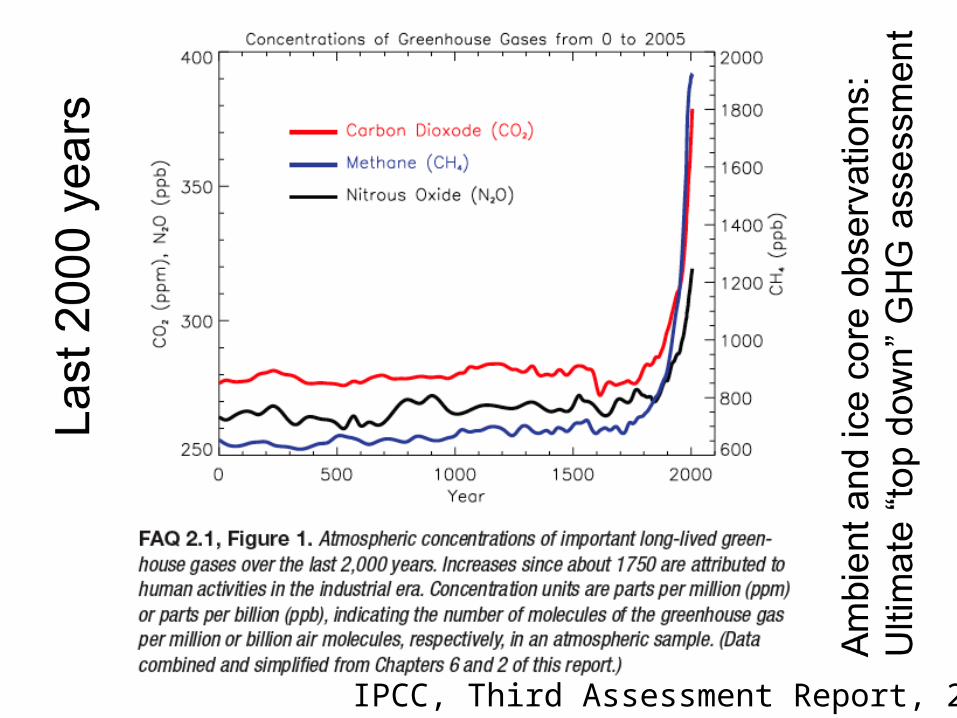
IPCC, Third Assessment Report, 2001

Global context

• Human activity is driving the greenhouse gas (GHG) content of the atmosphere far beyond anything seen for at least 600,000 years.

• Large reductions in GHG emissions will be needed to stabilize climate, even at 2K global warming (current <1K).– What level of mobile source GHG emissions

is tolerable?

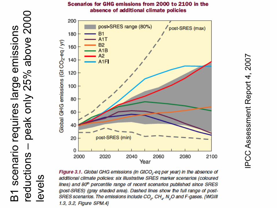
B1 scenario limits global warming to ~2K by 2100

IPCC Assessment Report 4, 2007

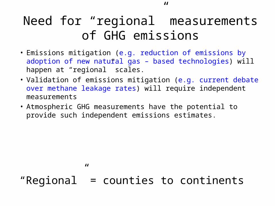
Need for “regional” measurements of GHG emissions

• Emissions mitigation (e.g. reduction of emissions by adoption of new natural gas – based technologies) will happen at “regional” scales.

• Validation of emissions mitigation (e.g. current debate over methane leakage rates) will require independent measurements

• Atmospheric GHG measurements have the potential to provide such independent emissions estimates.

“Regional” = counties to continents

Atmospheric methods: A very brief summary

Summary of Atmospheric Emissions Measurement Methods:Gaps between Chamber/Turbulent Flux and Inversion Methods

6

GAP

Cha

mbe

r flu

x

Eddy covarianceorPlume dispersion

Airborne flux

Global

year

month

hour

day

Tim

e S

cale

Spatial Scale

(1m)2 = 10-4ha

(1000km)2 = 108ha

(100km)2 = 106ha

(10km)2 = 104ha

(1km)2 = 102ha

Rearth

Regional

Atmospheric Inversions

Bridging the gap between atmospheric inversions and turbulent flux measurements is my research expertise.

“Handshakes” needed

• Combine regional estimates to match global budget

• Combine chamber and/or turbulent flux estimates to match regional budget (e.g. CH4 bottom up / top down comparison)

• Must consider not just total emissions, but also emissions source (e.g. agriculture, gas production, wetlands, gas seeps)

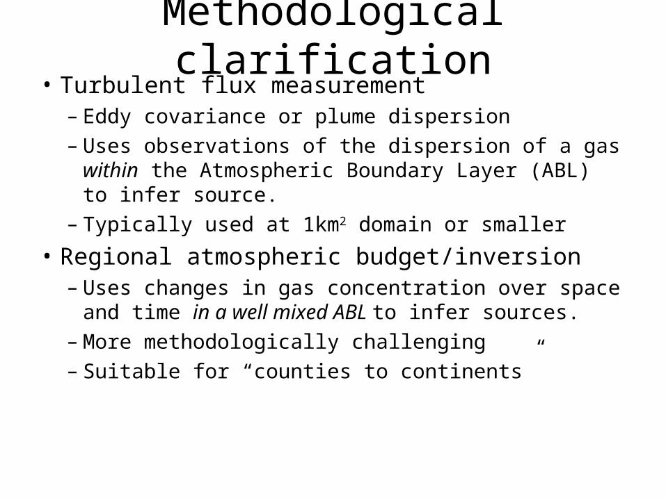
Methodological clarification• Turbulent flux measurement

– Eddy covariance or plume dispersion– Uses observations of the dispersion of a gas within the

Atmospheric Boundary Layer (ABL) to infer source.– Typically used at 1km2 domain or smaller

• Regional atmospheric budget/inversion– Uses changes in gas concentration over space and

time in a well mixed ABL to infer sources.– More methodologically challenging– Suitable for “counties to continents”

Regional atmospheric budgets:a part of the needed toolbox of methods

• Aircraft budgets– Excellent spatial coverage– Limited temporal coverage

• Tower (or satellite) based atmospheric inversions– Excellent temporal coverage– Spatial coverage (domain, resolution) limited

by density of long-term measurement network

Regional atmospheric measurements of CH4 (and CO2) sources and sinks

Regions of NOAA aircraft emissions estimates for natural gas production

Uinta, UTKarion et al. 2013 (8.9%)

Denver Julesburg, COPetron et al. 2012 (4%)Petron et al. submitted Marcellus,

PA/NYOngoing work

Barnett, TXKarion et al. in prep

Haynesville, LA/TXPeischl et al. in prep

Fayetteville, OKPeischl et al. in prep

% values are estimated leakage rates as a fraction of production

Penn State regional tower-based Penn State regional tower-based measurement campaignsmeasurement campaigns

Midcontinent intensive, 2007-2009.Richardson et al (2012)Miles et al (2012)Lauvaux et al (2012a,b)Schuh et al (2013)Lauvaux and Davis, 2013Diaz et al, in review

INFLUX, 2010-201?Pubs in prep

Gulf coast intensive(?), 2014-2016.Funds pending.N. American tower GHG network circa 2008

N. Marcellus. 2014-2016Deployment stage

Aircraft Mass Balance Method

b

b

z

z

airCHCH dxdznXVnPBL

gnd

44cos

Perpendicular wind speed

Wind

emissions

Wind

Background CH4

Downwind CH4

CH4 flux Molar CH4 enhancement in PBL

References: White et al., 1976; Ryerson et al., 2001; Mays et al., 2009

mixing height(PBL)

June 1, 2011 Flight path

Cambaliza et al, in reviewINFLUX, Purdue/Shepson group

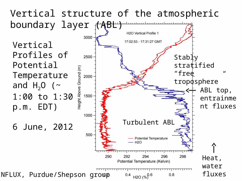
Vertical Profiles of Potential Temperature and H2O (~ 1:00 to 1:30 p.m. EDT)

6 June, 2012

Vertical structure of the atmospheric boundary layer (ABL)

Turbulent ABL

ABL top, entrainment fluxes

Stably stratified “free troposphere”

Heat, water fluxes

INFLUX, Purdue/Shepson group

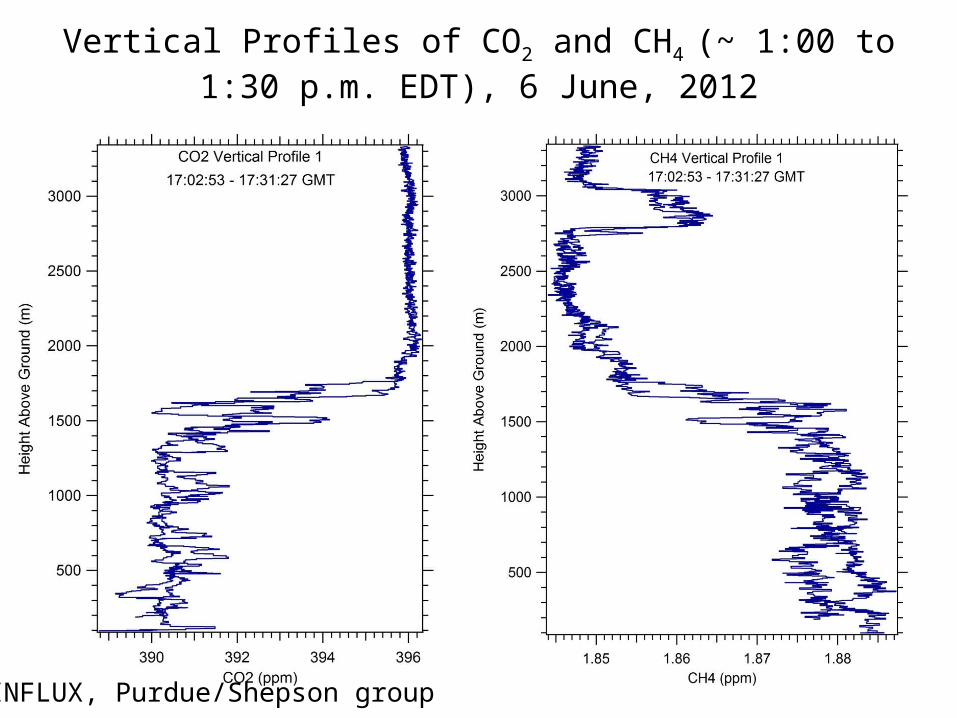
Vertical Profiles of CO2 and CH4 (~ 1:00 to 1:30 p.m. EDT), 6 June, 2012

INFLUX, Purdue/Shepson group

22,000 moles s-1 203 moles s-1

June 1, 2011 Results

Cambaliza et al, in reviewINFLUX, Purdue/Shepson group

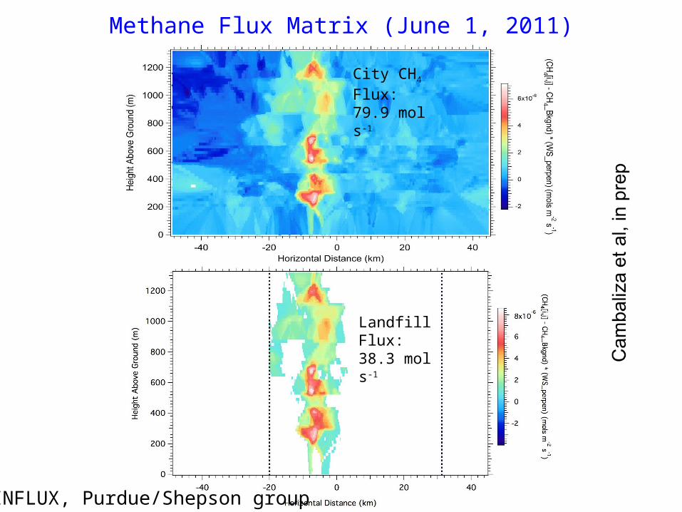
Methane Flux Matrix (June 1, 2011)

City CH4 Flux: 79.9 mol s-1

Landfill Flux: 38.3 mol s-1

INFLUX, Purdue/Shepson group

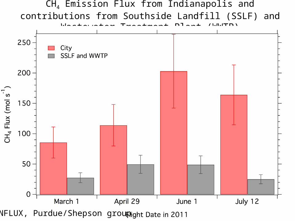
CH4 Emission Flux from Indianapolis and contributions from Southside Landfill (SSLF) and Wastewater Treatment Plant (WWTP)

INFLUX, Purdue/Shepson group

Utah, 2012

Distance perpendicular to wind (km)

CH

4 (

ppb

) downwind

upwind

Karion et al. 2013

HRDL

NOAA/Sweeney group

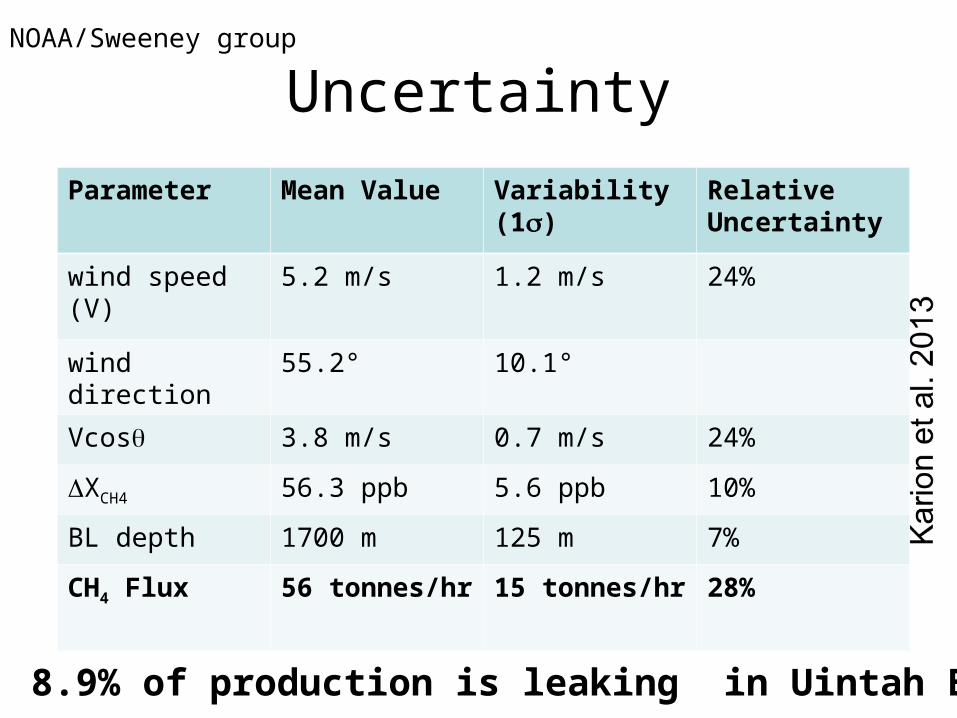
Uncertainty

Parameter Mean Value Variability (1) Relative Uncertainty

wind speed (V) 5.2 m/s 1.2 m/s 24%

wind direction 55.2° 10.1°

Vcos 3.8 m/s 0.7 m/s 24%

XCH4 56.3 ppb 5.6 ppb 10%

BL depth 1700 m 125 m 7%

CH4 Flux 56 tonnes/hr 15 tonnes/hr 28%

8.9% of production is leaking in Uintah Basin

NOAA/Sweeney group

Trace gases for attribution

• Ethane, propane, butane – associated with natural gas sources, but not agriculture or wetland sources

• 13CH4 – different sources have different isotopic ratios

• CO – associated with combustion

NOAA/Sweeney group

Conclusions: Airborne budgets• Powerful regional "snapshots" of total emissions -

moderate levels of uncertainty.

• CH4 source types can often be disaggregated with trace gases or source location data.

• Estimates to date suggest bottom-up methods underestimate total CH4 emissions. Why? Not clear at this point.

• Temporal variability difficult to capture. But if you sample a large enough area, perhaps statistics are in your favor.

• Little info on spatial distribution of emissions within the "box."

Tower-based “atmospheric inversion” CO2 (and CH4) source and sink estimates

Penn State regional tower-based Penn State regional tower-based measurement campaignsmeasurement campaigns

Midcontinent intensive, 2007-2009.Richardson et al (2012)Miles et al (2012)Lauvaux et al (2012a,b)Schuh et al (2013)Lauvaux and Davis, 2013Diaz et al, in review

INFLUX, 2010-201?Pubs in prep

Gulf coast intensive(?), 2014-2016.Funds pending.N. American tower GHG network circa 2008

N. Marcellus. 2014-2016Deployment stage

INFLUX objectives

• Develop improved methods for determination of urban area-wide, and spatially and temporally-resolved (e.g. monthly, 1 km2 resolution) fluxes of greenhouse gases, specifically, CO2 and CH4.

• Determine and minimize the uncertainty in the emissions estimate methods.

Observational system• 12 surface towers measuring CO2 mixing ratios, 5 with

CH4, and 5 with CO. (Penn State)

• 4 eddy-flux towers from natural to dense urban landscapes. (Penn State)

• 5 automated flask samplers. (NOAA/CU)• Periodic aircraft flights (~monthly) with CO2, CH4, and

flask samples. (Purdue / NOAA)• Periodic automobile surveys of CO2 and CH4. (Purdue)• Doppler lidar. (NOAA/CU)• TCCON-FTS for 4 months (Sept-Dec 2012). (NASA

Ames)

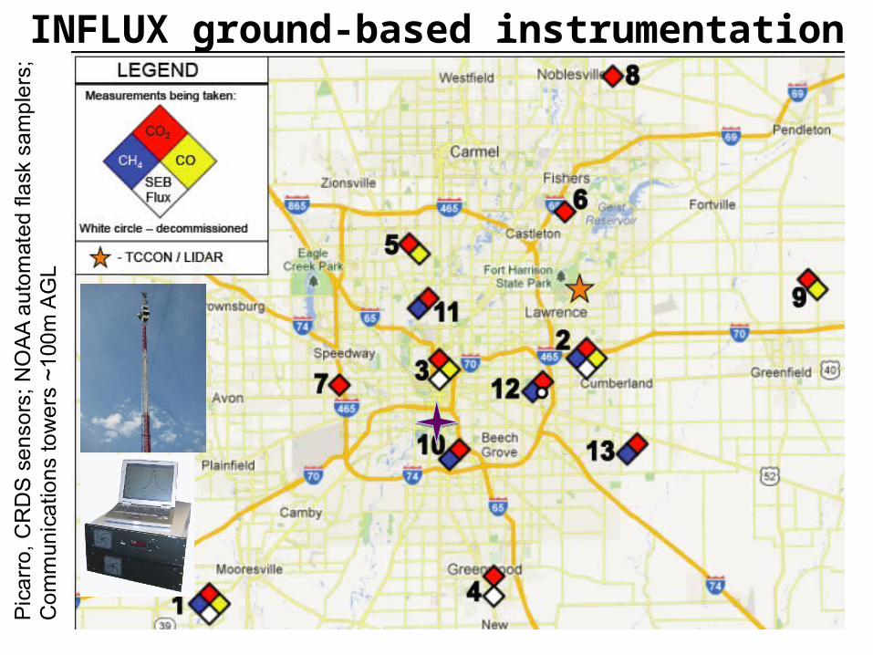
INFLUX ground-based instrumentation

Atmospheric inversions 101

• Take a first guess at emissions

• Transport these through the atmosphere using an atmospheric model (reanalysis)

• Compute CH4 at measurement points

• Compare modeled and observed CH4

• Adjust first guess of emissions to minimize the difference between observed and modeled CH4.

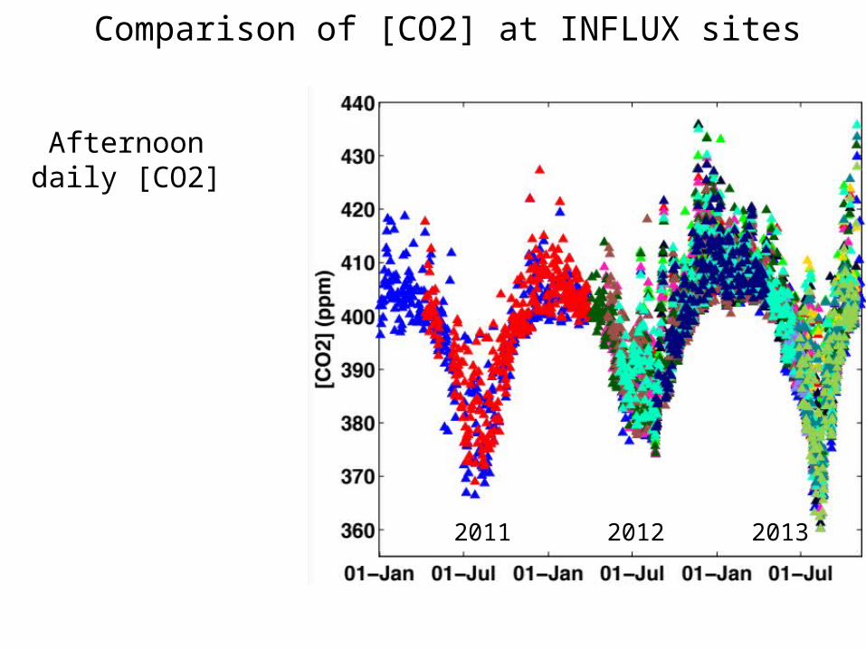
Comparison of [CO2] at INFLUX sites

2011 2012 2013

Afternoon daily [CO2]

• Afternoon [CO2] with 21-day smoothing

• Site 03 (downtown): high [CO2]

• Site 01 (background): low [CO2]

• Seasonal and synoptic cycles are evident

Comparison of [CO2] at INFLUX sites

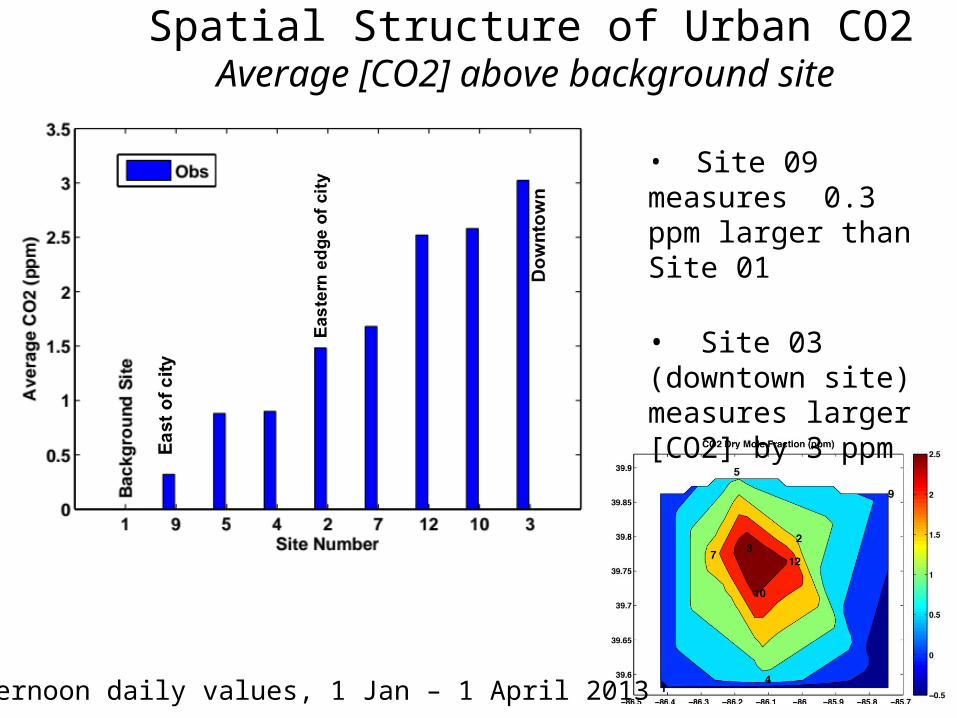
• Site 09 measures 0.3 ppm larger than Site 01

• Site 03 (downtown site) measures larger [CO2] by 3 ppm

Spatial Structure of Urban CO2Average [CO2] above background site

Afternoon daily values, 1 Jan – 1 April 2013

Vulcan and Hestia Emission Inventories / Models

Vulcan – hourly, 10km resolution for USA

Hestia: high resolution emission data for the residential, commercial and industrial sectors, in addition to the transportation and electricity production sectors.

•See: Kevin Gurney/•http://hestia.project.asu.edu/

250m res - Indy.

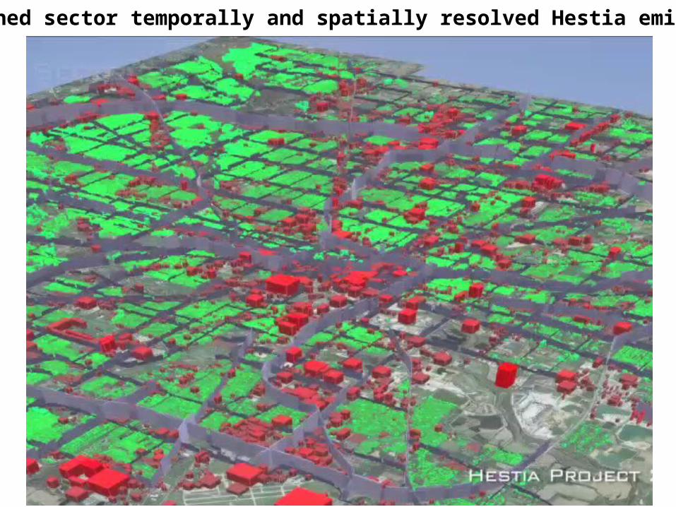
Combined sector temporally and spatially resolved Hestia emissions

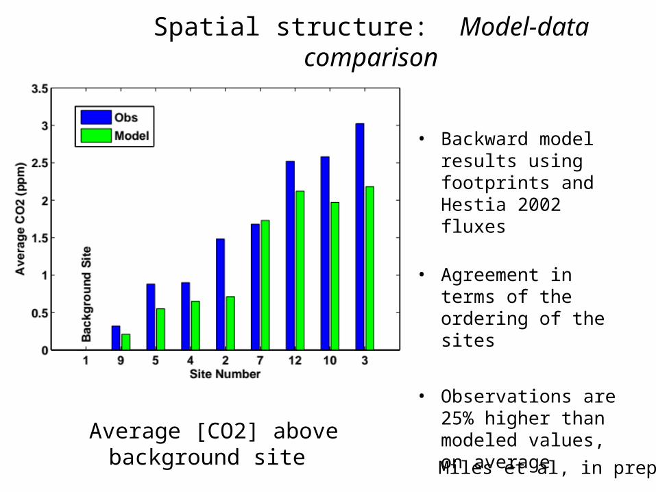
• Backward model results using footprints and Hestia 2002 fluxes

• Agreement in terms of the ordering of the sites

• Observations are 25% higher than modeled values, on average

Average [CO2] above background site

Spatial structure: Model-data comparison

Miles et al, in prep

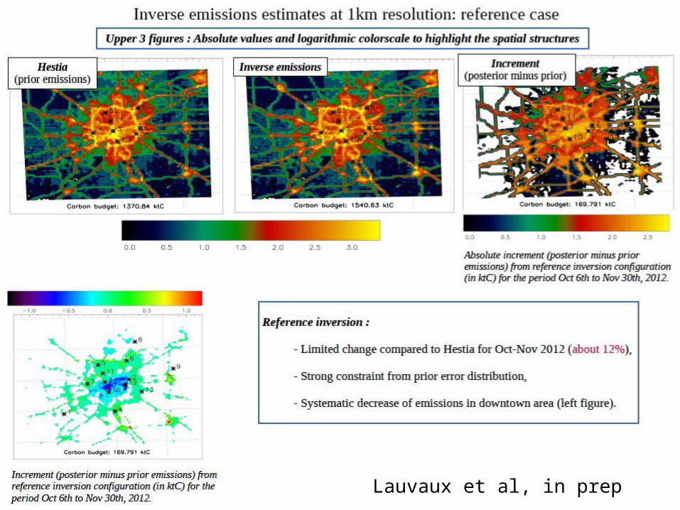
Lauvaux et al, in prep

CH4 Enhancement (Site 02 – Site 01) as a Function of Wind Direction

April – November 2011 (Afternoon hours only)

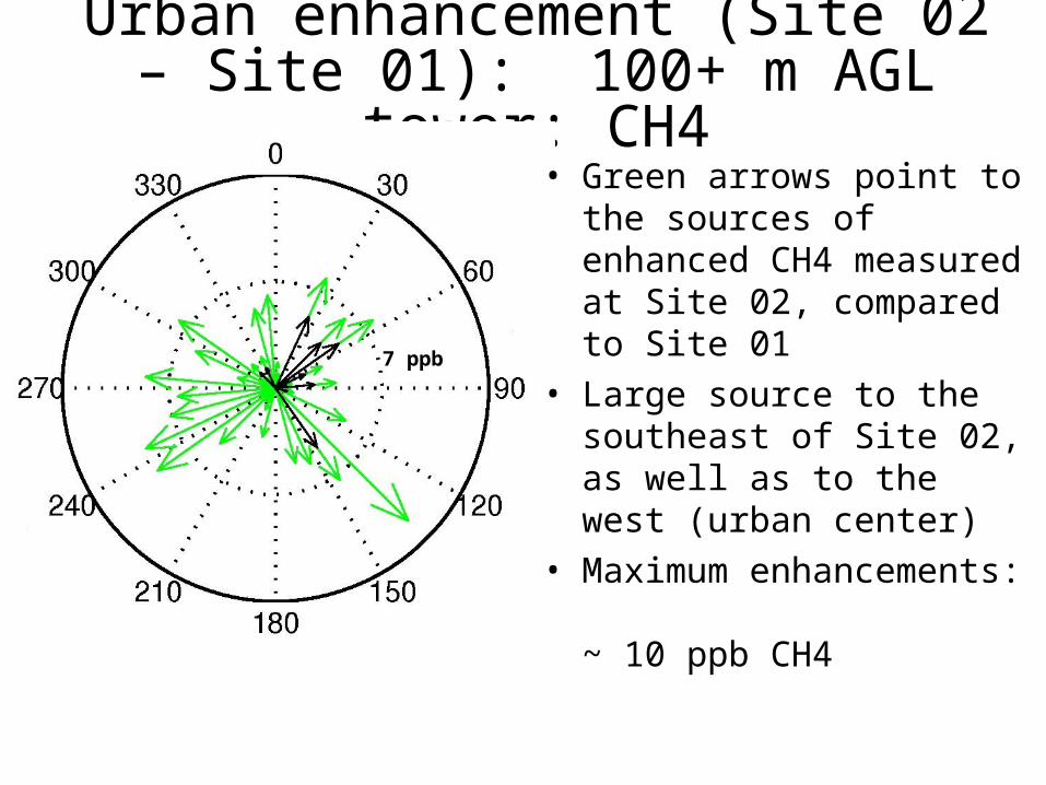
Urban enhancement (Site 02 – Site 01): 100+ m AGL tower: CH4

7 ppb

• Green arrows point to the sources of enhanced CH4 measured at Site 02, compared to Site 01

• Large source to the southeast of Site 02, as well as to the west (urban center)

• Maximum enhancements: ~ 10 ppb CH4

Conclusions: Atm inversions• Capture total emissions, like airborne mass balance. strength

and weakness.• Can be used to quantify temporal variability in emissions over

years• Sources can be disaggregated via 1) trace gases or 2) prior

knowledge of location and time of emissions.• Can provide spatially resolve emissions - given sufficient

atmospheric data density.• “Footprints" are still relatively small and dependent on wind

direction. • Uncertainty assessment is complex, but MCI results show

inversion uncertainties equal to those of agricultural inventories (Schuh et al., 2013).

Conclusions: Atm inversions

• INFLUX and N. Marcellus experiments are attempting to bring together (relatively) rigorous top-down and bottom-up assessments, and include both airborne and tower-based atmospheric inversions.

Overall summary• Comparisons across methods / scales are important to gather

understanding of the true net impacts on the global budget.

• Constructing a rigorous comparison is challenging.

• Aircraft are great for covering space, and for simple methods/uncertainty assessment, but are poor for temporal sampling.

• Towers are great for long-term monitoring and temporal variability, but the methodology is complex.

• In both cases, high measurement accuracy is required and sensors are costly.

• The effort is important - reducing GHG emissions is critical – we need to achieve (and verify) large reductions in C emissions.