Embed Size (px)
Citation preview
Atmospheric Mass Loss During Planet Formation: The
Importance of Planetesimal Impacts
Hilke E. Schlichting1, Re’em Sari2 and Almog Yalinewich2
ABSTRACT
Quantifying the atmospheric mass loss during planet formation is crucial for
understanding the origin and evolution of planetary atmospheres. We examine
the contributions to atmospheric loss from both giant impacts and planetesimal
accretion. Giant impacts cause global motion of the ground. Using analytic
self-similar solutions and full numerical integrations we find (for isothermal at-
mospheres with adiabatic index γ = 5/3) that the local atmospheric mass loss
fraction for ground velocities vg . 0.25vesc is given by χloss = (1.71vg/vesc)4.9,
where vesc is the escape velocity from the target. Yet, the global atmo-
spheric mass loss is a weaker function of the impactor velocity vImp and mass
mImp and given by Xloss ' 0.4x + 1.4x2 − 0.8x3 (isothermal atmosphere) and
Xloss ' 0.4x+ 1.8x2 − 1.2x3 (adiabatic atmosphere), where x = (vImpm/vescM).
Atmospheric mass loss due to planetesimal impacts proceeds in two different
regimes: 1) Large enough impactors m &√
2ρ0(πhR)3/2 (25 km for the current
Earth), are able to eject all the atmosphere above the tangent plane of the im-
pact site, which is h/2R of the whole atmosphere, where h, R and ρ0 are the
atmospheric scale height, radius of the target, and its atmospheric density at
the ground. 2) Smaller impactors, but above m > 4πρ0h3 (1 km for the current
Earth) are only able to eject a fraction of the atmospheric mass above the tangent
plane. We find that the most efficient impactors (per unit impactor mass) for at-
mospheric loss are planetesimals just above that lower limit (2 km for the current
Earth). For impactor flux size distributions parametrized by a single power law,
N(> r) ∝ r−q+1, with differential power law index q, we find that for 1 < q < 3
the atmospheric mass loss proceeds in regime 1) whereas for q > 3 the mass loss
is dominated by regime 2). Impactors with m . 4πρ0h3 are not able to eject
any atmosphere. Despite being bombarded by the same planetesimal population,
1Massachusetts Institute of Technology, 77 Massachusetts Avenue, Cambridge, MA 02139-4307, USA
2Racah Institute of Physics, Hebrew University, Jerusalem 91904, Israel
arX
iv:1
406.
6435
v2 [
astr
o-ph
.EP]
26
Aug
201
4
– 2 –
we find that the current differences in Earth’s and Venus’ atmospheric masses
can be explained by modest differences in their initial atmospheric masses and
that the current atmosphere of the Earth could have resulted from an equilib-
rium between atmospheric erosion and volatile delivery to the atmosphere from
planetesimal impacts. We conclude that planetesimal impacts are likely to have
played a major role in atmospheric mass loss over the formation history of the
terrestrial planets.
Subject headings: planetary systems: general — planets and satellites: formation
— solar system: formation
1. INTRODUCTION
Terrestrial planet formation is generally thought to have proceeded in two main stages:
The first consists of the accretion of planetesimals, which leads to the formation of several
dozens of roughly Mars-sized planetary embryos (e.g. Ida & Makino 1993; Weidenschilling
et al. 1997), and the second stage consists of a series of giant impacts between these embryos
that merge to form the Earth and other terrestrial planets (e.g. Agnor et al. 1999; Chambers
2001). Understanding how much of the planets’ primordial atmosphere is retained during
the giant impact phase is crucial for understanding the origin and evolution of planetary at-
mospheres. In addition, a planet’s or proptoplanet’s atmosphere cannot only be lost due to
a collision with a comparably sized body in a giant impact, but also due to much smaller im-
pacts by planetesimals. During planet formation giant impacts begin when the planetesimals
are no longer able to efficiently damp the eccentricities of the growing protoplanets. Order
of magnitude estimates that balance the stirring rates of the protoplanets with the damping
rates due to dynamical friction by the planetesimal population and numerical simulations
find that giant impacts set in when the total mass in protoplanets is comparable to the mass
in planetesimals (Goldreich et al. 2004; Kenyon & Bromley 2006). Therefore about 50%
of the total mass still resides in planetesimals when giant impacts begin and planetesimal
accretion continues throughout the giant impact phase. Furthermore, geochemical evidence
from highly siderophile element (HSE) abundance patterns inferred for the terrestrial planets
and the Moon suggest that a total of about 0.01 M⊕ of chondritic material was delivered as
‘late veneer’ by planetesimals to the terrestrial planets after the end of giant impacts (War-
ren et al. 1999; Walker et al. 2004; Walker 2009). This suggests that planetesimal accretion
did not only proceed throughout the giant impacts stage by continued beyond. Therefore,
in order to understand the origin and evolution of the terrestrial planets’ atmospheres one
needs to examine the contribution to atmospheric loss from both the giant impacts and from
– 3 –
planetesimal accretion.
Depending on impactor sizes, impact velocities and impact angles, volatiles may be
added to or removed from growing planetary embryos by impacts of other planetary embryos
and smaller planetesimals. The survival of primordial atmospheres through the stage of giant
impacts during terrestrial planet formation has been examined by Genda & Abe (2003) and
Genda & Abe (2005). These works numerically integrate the hydrodynamic equations of
motion of the planetary atmosphere to determine the amount of atmospheric loss for various
ground velocities. In contrast to giant impacts, smaller impactors cannot eject the planet’s
atmosphere globally but are limited to, at best, ejecting all the atmosphere above the tangent
plane of the impact site. Some of the first calculations of impact induced atmospheric erosion
were performed using the Zel’dovich & Raizer (1967) solution for the expansion of a vapor
plume and momentum balance between the expanding gas and the mass of the overlying
atmosphere (e.g. Melosh & Vickery 1989; Vickery & Melosh 1990; Ahrens 1993). The results
of these calculations were used to investigate the evolution of planetary atmospheres as
a result of planetesimal impacts (e.g. Zahnle et al. 1990, 1992). Newman et al. (1999)
investigated by analytical and computational means the effect of ∼ 10 km impactors on
terrestrial atmospheres using an analytical model based on the solutions of Kompaneets
(1960). Atmospheric erosion calculations were extended further by, for example, Svetsov
(2007) and Shuvalov (2009) who investigated numerically atmospheric loss and replenishment
and the role of oblique impacts, respectively. In the work presented here, we use order of
magnitude estimates and numerical simulations to calculate the atmospheric mass loss over
the entire range of impactor sizes, spanning impacts too small to eject significant amounts of
atmosphere to planetary-embryo scale giant impacts. Our results demonstrate that the most
efficient impactors (per impactor mass) for atmospheric loss are small planetesimals which,
for the current atmosphere of the Earth, are only about 2 km in radius. We show that these
small planetesimal impacts could have potentially totally dominated the atmospheric mass
loss over Earth’s history and during planet formation in general.
Our paper is structured as follows: In section 2 we use analytic self-similar solutions and
full numerical integrations to calculate the amount of atmosphere lost during giant impacts
for an isothermal and adiabatic atmosphere. We analytically calculate the atmospheric
mass loss due to planetesimal impacts in section 3. In section 4, we compare and contrast
the atmospheric mass loss due to giant impacts and planetesimal accretion and show that
planetesimal impacts likely played a more important role for atmospheric loss of terrestrial
planets than giant impacts. We discuss the implications of our results for terrestrial planet
formation and compare our findings with recent geochemical constraints on atmospheric loss
and the origin of Earth’s atmosphere in section 5. Discussion and conclusions follow in
section 6.
– 4 –
2. Atmospheric Mass Loss Due to Giant Impacts
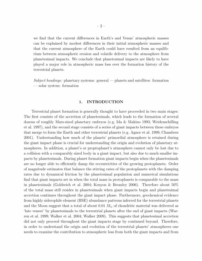
When an impact occurs the planet’s atmosphere can be lost in two distinct ways: First,
the expansion of plumes generated at the impact site can expel the atmosphere locally but
not globally. Atmospheric loss is therefore limited to at best h/(2R) of the total atmosphere,
where h is the atmospheric scale height and R the planetary radius (see section 3 for details).
Second, giant impacts create a strong shock that propagates through the planetary interior
causing a global ground motion of the proto-planet. This ground motion in turn launches a
strong shock into the planetary atmosphere, which can lead to loss of a significant fraction
of or even the entire atmosphere.
Fig. 1.— Illustration of a giant impact. 1) The giant impact ejects atmosphere and ejecta
close to the impact point and launches a strong shock. 2) The shock front propagates through
the target causing a global ground motion. 3) This ground motion in turn launches a strong
shock into the planetary atmosphere, which can lead to loss of a significant fraction of or
even the entire atmosphere.
It was realized several decades ago that self-similar solutions provide an excellent de-
– 5 –
scription for a shock propagating in adiabatic and isothermal atmospheres (e.g. Raizer 1964;
Grover & Hardy 1966). Here, we take advantage of these self-similar solutions and use them
together with full numerical integrations to calculate the atmospheric mass loss due to giant
impacts.
2.1. Self-Similar Solutions to the Hydrodynamic Equations for an Isothermal
Atmosphere
Terrestrial planet’s atmospheres, like the Earth’s, are to first order isothermal, giving
rise to an exponential density profile. We therefore solve the hydrodynamic equations for a
shock propagating in an atmosphere with an exponential density profile given by
ρ = ρ0 exp[−z/h], (1)
where ρ0 is the density on the ground, z the height in the atmosphere measured from the
ground and h the atmospheric scale height. The atmosphere is assumed to be planar, which
is valid for the terrestrial planets since their atmospheric scale heights are small compared
to their radii. We further assume that radiative losses can be neglected such that the flow
is adiabatic. The adiabatic hydrodynamic equations are given by
1
ρ
Dρ
Dt+∂u
∂z= 0 (2)
Du
Dt+
1
ρ
∂p
∂z= 0 (3)
1
p
Dp
Dt− γ
ρ
Dρ
Dt= 0, (4)
where γ is the adiabatic index and D/Dt the ordinary Stokes time derivative.
Thanks to the self-similar behavior of the flow, the solutions to hydrodynamic equations
above can be separated into their time-dependent and spatial parts and can be written as
ρ(z, t) = ρ0 exp[−Z(t)/h]G(ζ), u(z, t) = ZU(ζ), p(z, t) = ρ0 exp[−Z(t)/h]Z2P (ζ) (5)
where Z(t) is the position of the shock front and ζ = (z − Z(t))/h. The similarity variables
for the density, velocity and pressure are given by G(ζ), U(ζ) and P (ζ), respectively. Using
the expressions in Equation (5) and substituting them into the hydrodynamic Equations
(2)-(4) yields for the spatial parts
1
G
dG
dζ(U − 1) +
dU
dζ= 1 (6)
– 6 –
(U − 1)dU
dζ+
1
G
dP
dζ= −U
α(7)
(U − 1)
(1
P
dP
dζ− γ
G
dG
dζ
)= − 2
α− γ + 1, (8)
and a time dependent part given byZ2
Z= αh. (9)
Using the strong shock conditions we have
G(0) =γ + 1
γ − 1, U(0) =
2
γ + 1, P (0) =
2
γ + 1. (10)
Having separated the hydrodynamic equations into their time-dependent and spatial
parts and we now obtain their self-similar solution. The solution to Equation (9) yields the
position of the shock front as a function of time and is given by
Z(t) = −αh ln [1− (t/t0)] (11)
where t0 = 2αh/[vg(γ+ 1)] and vg is the ground velocity at the interface between the ground
the atmosphere. Equation (11) shows that the shock accelerates fast enough such that it
arrives at infinity in time t0. The ground in contrast only transverses a distance 2αh/(γ+1),
which is a few scale heights, in the same time.
Although various solutions to Equations (6)-(8) exist for different values of α, the phys-
ically relevant solution corresponds to a unique value of α which allows passage through a
critical point, ζc. This critical point corresponds to the sonic point in the time-dependent
flow. Self-smilar solutions that include passage trough the sonic point are generally referred
to as type II self-similar solutions. For example, we find, consistent with previous works
(Grover & Hardy 1966; Chevalier 1990), that for γ = 4/3, α = 5.669 and the critical point
is located at ζc = −0.356 and similarly, for γ = 5/3, α = 4.892 and ζc = −0.447. Since
the self-similar solutions have to pass through the sonic point, only the region between the
shock front and the sonic point are in communication and the part of the flow beyond the
sonic point is cut off. The beauty of this is that the solution of the hydrodynamic equations
becomes independent of the detailed nature of the initial shock conditions, such that the ve-
locity of the ground motion that launches the shock only enters in the form of multiplicative
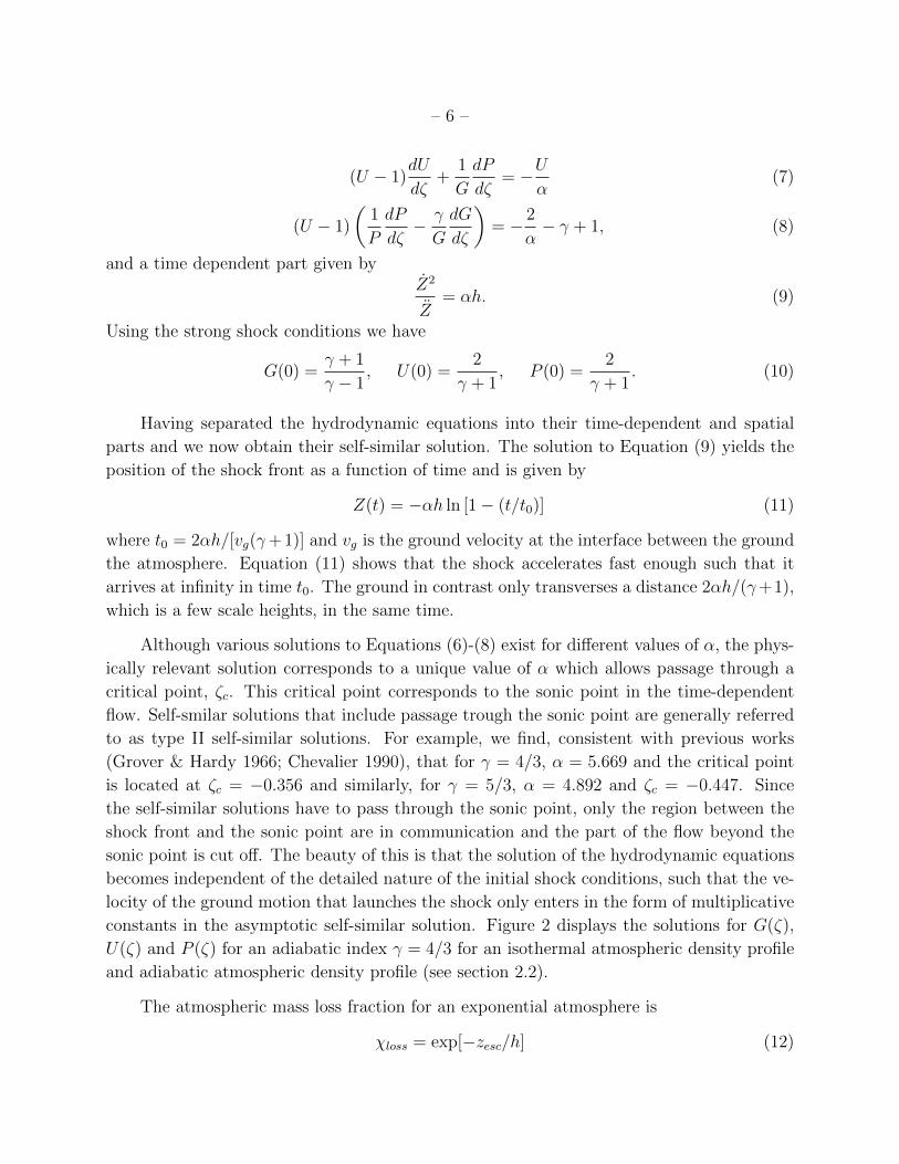
constants in the asymptotic self-similar solution. Figure 2 displays the solutions for G(ζ),
U(ζ) and P (ζ) for an adiabatic index γ = 4/3 for an isothermal atmospheric density profile
and adiabatic atmospheric density profile (see section 2.2).
The atmospheric mass loss fraction for an exponential atmosphere is
χloss = exp[−zesc/h] (12)
– 7 –
-1.0 -0.8 -0.6 -0.4 -0.2 0.0
0
50
100
150
200
250
Ζ
GHΖL
-1.0 -0.8 -0.6 -0.4 -0.2 0.00.3
0.4
0.5
0.6
0.7
0.8
0.9
Ζ
UHΖL
-1.0 -0.8 -0.6 -0.4 -0.2 0.0
1
2
3
4
Ζ
PHΖL
Fig. 2.— Solutions for G(ζ), U(ζ) and P (ζ) for an adiabatic index γ = 4/3 for an adiabatic
atmospheric density profile, ρ = ρ0(1 − z/z0)n with n = 1.5, (solid line) and an isothermal
atmospheric density profile, ρ = ρ0 exp[−z/h], (dashed line).
– 8 –
where zesc is the initial height in the atmosphere of the fluid element that has a velocity equal
to the escape velocity at a time long after the shock has passed, such that the atmosphere at
z ≥ zesc will be lost. From Equation (11) we have that the shock velocity grows exponentially
with height in the atmosphere just as the density deceases exponentially. The shock velocity
is given by
Z =γ + 1
2vg exp[z/αh]. (13)
zesc can therefore be written as vesc = vgβ exp[zesc/αh] where vesc is the escape velocity of
the impacted body and β is a numerical constant that relates the velocity of a given fluid
element at a time long after the shock has passed, u∞, to the velocity of the same fluid
element at the shock, u0. The final atmospheric mass loss fraction is therefore
χloss =
(βvgvesc
)α, (14)
where the only quantity left to calculate numerically is the acceleration factor β given by
β =u∞u0. (15)
It is convenient to write β as the product of the acceleration factor until the shock has reached
infinity (ut0/u0), which happens at time t0, and the acceleration factor from the time that
the shock reached ∞ to a long time after that (u∞/ut0), such that β = (u∞/ut0)(ut0/u0).
The latter is important because a given fluid element continues to accelerate after t0. The
two parts of the acceleration factor can be written as
ut0u0
=U(ζ → −∞)Z(ζ → −∞)
U(ζ = 0)Z(ζ = 0),
u∞ut0
=U(ζ → +∞)Z(ζ → +∞)
U(ζ → −∞)Z(ζ → −∞). (16)
Equations (16) required that we take the limit for ζ and t together. This is accomplished by
rewriting Z as d ln Z/dζ = (α(U(ζ)− 1))−1 and solving it together with Equations (6) - (8).
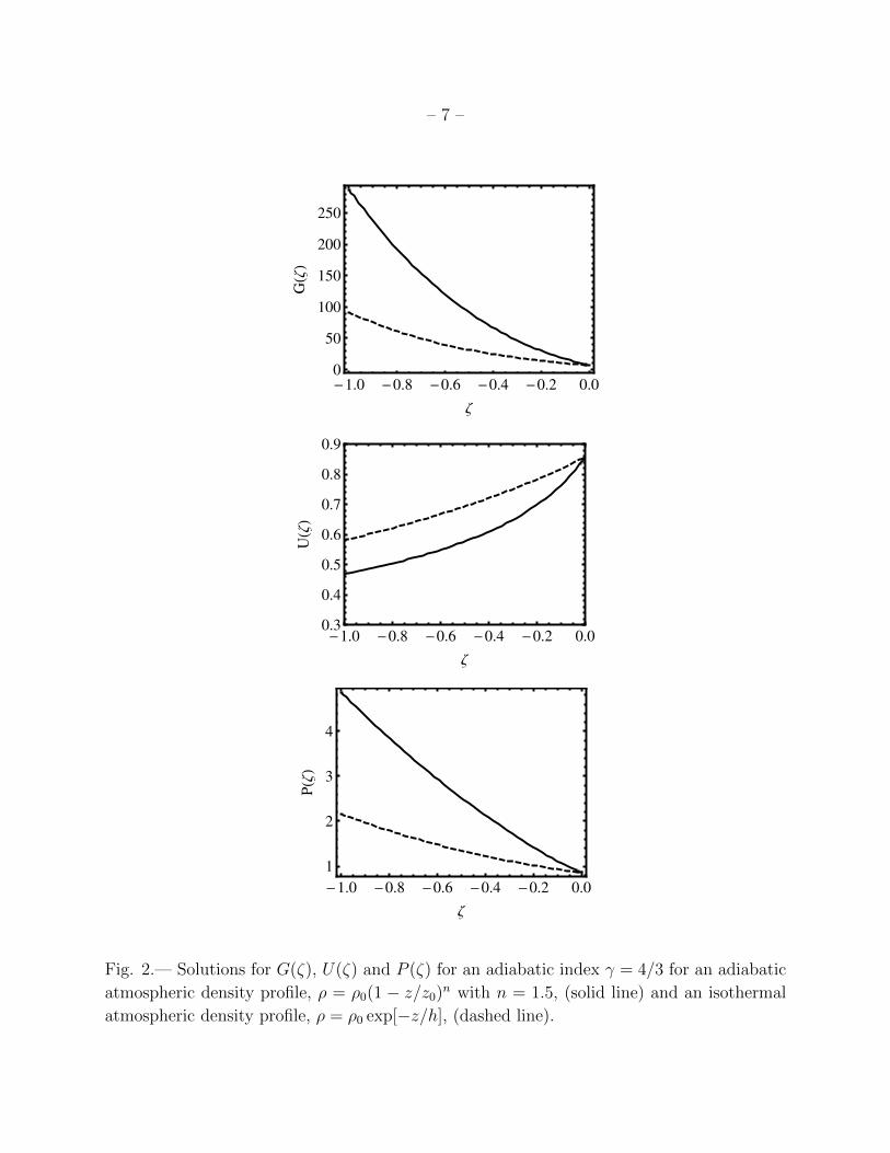
Figure 3 displays the two components of the acceleration factor and we find that β = 2.07
for γ = 4/3 and 1.90 for γ = 5/3.
Because the shock is not immediately self-similar from the very moment that it is
launched into the atmosphere, the actual acceleration factor, β, is less than the value of
β obtained from the self-similar solutions. Furthermore, the atmosphere close to the ground
is not accelerated as much as fluid elements with initial positions significantly above the
ground. Therefore, in order to obtain the actual value of β and an accurate atmospheric
mass loss for the part of the atmosphere that resides close to the ground, we performed full
numerical integrations of the hydrodynamic equations. The simulations were performed us-
ing the one dimensional version of RICH (Yalinewich et al., in preparation), a Godunov type

– 9 –
-20 -15 -10 -5 01.0
1.1
1.2
1.3
1.4
1.5
Ζ
u�u
0
Ρ=Ρ0exp-z�h, ý=4�3
Ρ=Ρ0exp-z�h, ý=5�3
Ρ=Ρ0H1-z�z0Ln, ý=5�3
Ρ=Ρ0H1-z�z0Ln, ý=4�3
Ρ=Ρ0exp-z�h, ý=4�3
Ρ=Ρ0exp-z�h, ý=5�3
Ρ=Ρ0H1-z�z0Ln, ý=5�3
Ρ=Ρ0H1-z�z0Ln, ý=4�3
Ρ=Ρ0exp-z�h, ý=4�3
Ρ=Ρ0exp-z�h, ý=5�3
Ρ=Ρ0H1-z�z0Ln, ý=5�3
Ρ=Ρ0H1-z�z0Ln, ý=4�3
Ρ=Ρ0exp-z�h, ý=4�3
Ρ=Ρ0exp-z�h, ý=5�3
Ρ=Ρ0H1-z�z0Ln, ý=5�3
Ρ=Ρ0H1-z�z0Ln, ý=4�3
0 100 200 300 4001.0
1.2
1.4
1.6
1.8
Ζ
u�u
t 0
Ρ=Ρ0exp-z�h, ý=4�3
Ρ=Ρ0exp-z�h, ý=5�3
Ρ=Ρ0H1-z�z0Ln, ý=5�3
Ρ=Ρ0H1-z�z0Ln, ý=4�3
Ρ=Ρ0exp-z�h, ý=4�3
Ρ=Ρ0exp-z�h, ý=5�3
Ρ=Ρ0H1-z�z0Ln, ý=5�3
Ρ=Ρ0H1-z�z0Ln, ý=4�3
Ρ=Ρ0exp-z�h, ý=4�3
Ρ=Ρ0exp-z�h, ý=5�3
Ρ=Ρ0H1-z�z0Ln, ý=5�3
Ρ=Ρ0H1-z�z0Ln, ý=4�3
Ρ=Ρ0exp-z�h, ý=4�3
Ρ=Ρ0exp-z�h, ý=5�3
Ρ=Ρ0H1-z�z0Ln, ý=5�3
Ρ=Ρ0H1-z�z0Ln, ý=4�3
Fig. 3.— Left: u/u0 as a function of distance form the shock front, ζ, for an isothermal (thin
lines) and adiabatic density profile (thick lines). The solid and dashed lines correspond to
γ = 4/3 and γ = 5/3, respectively. The value of acceleration factor until the shock reached
∞, ut0/u0, can be read of the left side of the figure corresponding to large distances from
the shock front. Right: u/ut0 as a function of ζ. The value of acceleration factor from the
time the shock reached ∞ until a long time after that, u∞/ut0 , can be read of the right
side on the figure corresponding to late times long after the shock front reached ∞. The
total acceleration factor, β, is the product of the ut0/u0 shown in the left Figure and u∞/ut0shown in the right Figure.
– 10 –
hydro-code on a moving Lagrangian mesh. We used a grid with a total of 1000 elements
and as boundary conditions we used a piston moving at a constant velocity on one side
and assumed a vacuum on the other. Due to numerical reasons, we couldn’t set the initial
upstream pressure to zero, so we used a small value of 10−9. We verified that the results
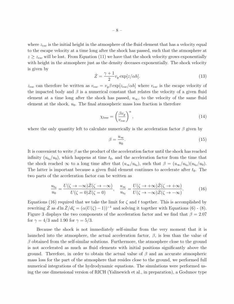
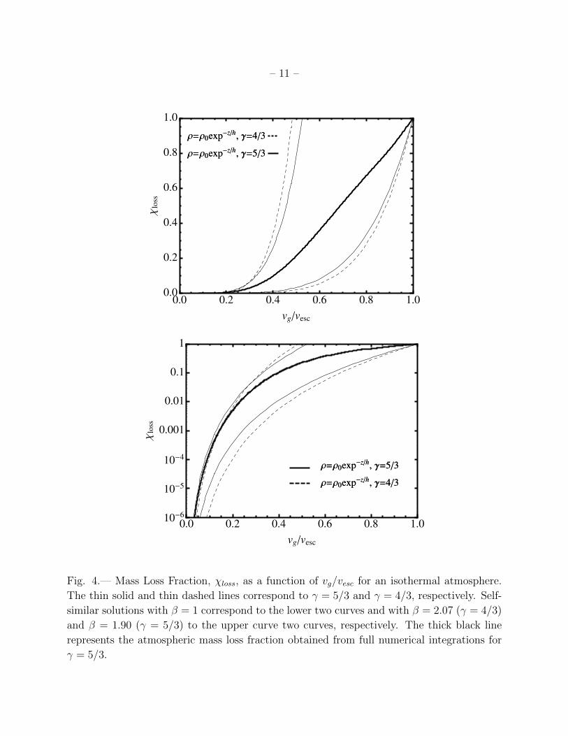
converged by running the same simulation with half as many grid points. Figure 4 shows the
atmospheric mass loss fraction, χloss, as a function of vg/vesc from our self-similar solutions
(thin lines) with β = 1 (lower curves) and β = 2.07 (γ = 4/3, dashed upper curve) and
β = 1.90 (γ = 5/3, solid upper curve). The numerical solution for γ = 5/3 is represented by
the thick line. As expected, the full numerical solution for γ = 5/3 falls between the β = 1
and β = 1.90 lines and we find that the actual value of β is 1.71.
Given the resulting distribution of ground velocities, vg, from a giant impact (see section
2.3), Equation (14) can be used to determine the global atmospheric mass loss fraction for
an isothermal atmosphere.
2.2. Self-Similar Solutions to the Hydrodynamic Equations for an Adiabatic
Atmosphere
The heat transport in many of the close-in exoplanet atmosphere may be dominated by
convection rather than radiation, resulting in adiabatic atmospheres. Unlike an isothermal
atmosphere, an adiabatic atmosphere has a density profile that reaches ρ = 0 at a finite
distance from the planet. Similar to the isothermal density profile considered above, we can
repeat our calculation for an atmosphere with an adiabatic density profile given by
ρ = ρ0(1− z/z0)n, (17)
where z0 is the edge of the atmosphere where ρ = 0 and P = 0 and n is the polytropic
index. We again assume that the atmosphere is planar and that radiative losses can be
neglected such that the flow is adiabatic. For the adiabatic density profile the solutions to
hydrodynamic equations above can again be separated into their time-dependent and spatial
parts and are given by
ρ(z, t) = ρ0(1−Z(t)/z0)nG(ζ), u(z, t) = ZU(ζ), p(z, t) = ρ0(1−Z(t)/z0)
nZ2P (ζ) (18)
where Z(t) is the position of the shock front and ζ = (z − Z(t))/(z0 − Z(t)).
Using the expressions in Equation (18) and substituting them into the hydrodynamic
Equations (2)-(4) yields for the spatial parts
1
G
dG
dζ(U − 1 + ζ) +
dU
dζ= n (19)
– 11 –
0.0 0.2 0.4 0.6 0.8 1.00.0
0.2
0.4
0.6
0.8
1.0
vg�vesc
Χlo
ss
Ρ=Ρ0exp-z�h, ý=4�3
Ρ=Ρ0exp-z�h, ý=5�3
Ρ=Ρ0exp-z�h, ý=4�3
Ρ=Ρ0exp-z�h, ý=5�3
0.0 0.2 0.4 0.6 0.8 1.010-6
10-5
10-4
0.001
0.01
0.1
1
vg�vesc
Χlo
ss
Ρ=Ρ0exp-z�h, ý=4�3
Ρ=Ρ0exp-z�h, ý=5�3
Ρ=Ρ0exp-z�h, ý=4�3
Ρ=Ρ0exp-z�h, ý=5�3
Fig. 4.— Mass Loss Fraction, χloss, as a function of vg/vesc for an isothermal atmosphere.
The thin solid and thin dashed lines correspond to γ = 5/3 and γ = 4/3, respectively. Self-
similar solutions with β = 1 correspond to the lower two curves and with β = 2.07 (γ = 4/3)
and β = 1.90 (γ = 5/3) to the upper curve two curves, respectively. The thick black line
represents the atmospheric mass loss fraction obtained from full numerical integrations for
γ = 5/3.
– 12 –
(U − 1 + ζ)dU
dζ+
1
G
dP
dζ= −U
α(20)
(U − 1 + ζ)
(1
P
dP
dζ− γ
G
dG
dζ
)= − 2
α− (γ − 1)n, (21)
and a time dependent part given by
Z2
Z(1− Z/z0)= αz0. (22)
Solving Equation (22) using the same strong shock initial conditions given in Equation (10)
yields for the position of the shock front as a function of time
Z(t) = z0
[1−
(1− t
t0
) α1+α
](23)
where t0 = 2z0α/(vg(1 + α)(1 + γ)) is the time at which the shock reaches the edge of the
atmosphere at z = z0.
Just like for the exponential atmosphere, the physically relevant solution to Equations
(19) - (21) for the adiabatic atmosphere density profile corresponds to a unique value of
α which allows passage through the critical point. We find, for γ = 4/3, α = 1.796 and
ζC = −0.083 and for γ = 5/3, α = 3.029 and ζC = −0.156. Figure 2 shows the solutions
for G(ζ), U(ζ) and P (ζ) for γ = 4/3 for an adiabatic atmospheric density profile (solid line)
and an isothermal atmospheric density profile (dashed line).
The atmospheric mass loss fraction for an adiabatic atmosphere is
χloss =
(1− zesc
z0
)n+1
(24)
where zesc is the initial height in the atmosphere of the fluid element that has a velocity
equal to the escape velocity at a time long after the schlock has passed. From Equation (23)
we have that the shock accelerates with height in the atmosphere and the shock velocity is
given by
Z =γ + 1
2vg
(1− z
z0
)−1/α. (25)
zesc can therefore be written as vesc = vgβ(1− zesc/z0)−1/α. β is again a numerical constant
that relates the velocity of a given fluid element at a time long after the shock has passed,
u∞, to the velocity of the same fluid element at the shock, u0. The final atmospheric mass
loss fraction is therefore
χloss =
(βvgvesc
)α(n+1)
. (26)
– 13 –
Calculating β using an analogous procedure to one employed for the isothermal atmosphere
in section 2.1 with the main difference that Z is now given by d ln Z/dζ = (α(U(ζ)−1+ζ))−1,
we find β = 2.38 and β = 2.27 for for γ = 4/3 and γ = 5/3, respectively. Figure 3 shows the
two components of the acceleration as a function of the distance from the shock front, ζ, for
an exponential and adiabatic atmospheric density profile.
Therefore, the exponent of βvg/vesc for an adiabatic atmosphere is, for example, 7.2
for n = 3 and γ = 4/3 and 7.6 for n = 1.5 and γ = 5/3 compared to 5.7 (γ = 4/3) and
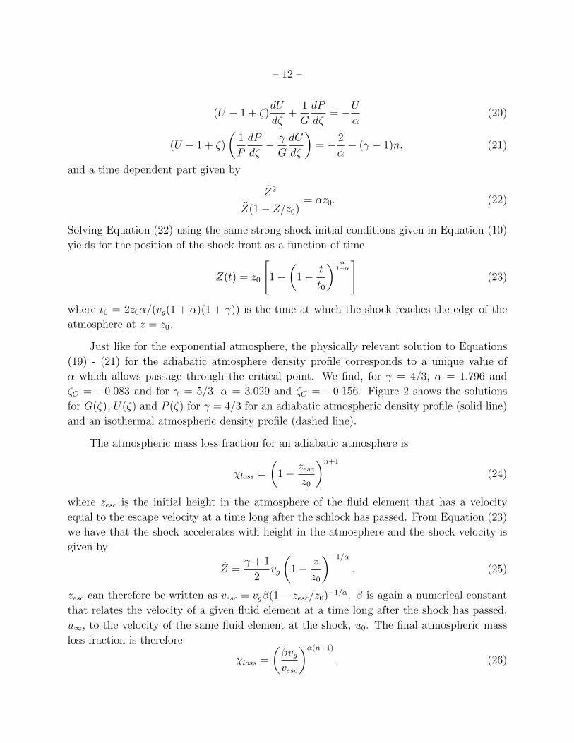
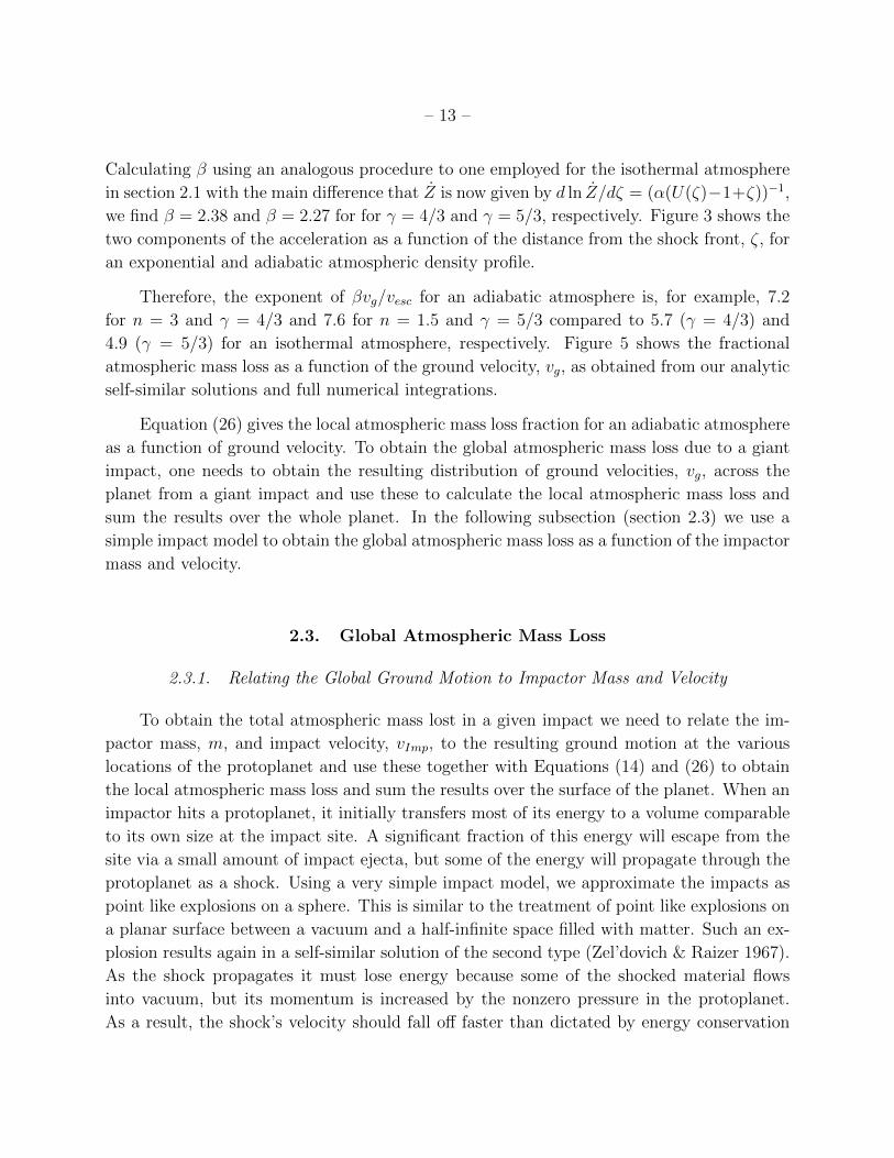
4.9 (γ = 5/3) for an isothermal atmosphere, respectively. Figure 5 shows the fractional
atmospheric mass loss as a function of the ground velocity, vg, as obtained from our analytic
self-similar solutions and full numerical integrations.
Equation (26) gives the local atmospheric mass loss fraction for an adiabatic atmosphere
as a function of ground velocity. To obtain the global atmospheric mass loss due to a giant
impact, one needs to obtain the resulting distribution of ground velocities, vg, across the
planet from a giant impact and use these to calculate the local atmospheric mass loss and
sum the results over the whole planet. In the following subsection (section 2.3) we use a
simple impact model to obtain the global atmospheric mass loss as a function of the impactor
mass and velocity.
2.3. Global Atmospheric Mass Loss
2.3.1. Relating the Global Ground Motion to Impactor Mass and Velocity
To obtain the total atmospheric mass lost in a given impact we need to relate the im-
pactor mass, m, and impact velocity, vImp, to the resulting ground motion at the various
locations of the protoplanet and use these together with Equations (14) and (26) to obtain
the local atmospheric mass loss and sum the results over the surface of the planet. When an
impactor hits a protoplanet, it initially transfers most of its energy to a volume comparable
to its own size at the impact site. A significant fraction of this energy will escape from the
site via a small amount of impact ejecta, but some of the energy will propagate through the
protoplanet as a shock. Using a very simple impact model, we approximate the impacts as
point like explosions on a sphere. This is similar to the treatment of point like explosions on
a planar surface between a vacuum and a half-infinite space filled with matter. Such an ex-
plosion results again in a self-similar solution of the second type (Zel’dovich & Raizer 1967).
As the shock propagates it must lose energy because some of the shocked material flows
into vacuum, but its momentum is increased by the nonzero pressure in the protoplanet.
As a result, the shock’s velocity should fall off faster than dictated by energy conservation
– 14 –
0.0 0.2 0.4 0.6 0.8 1.00.0
0.2
0.4
0.6
0.8
1.0
vg�vesc
Χlo
ss
Ρ=Ρ0H1-z�z0L3, ý=4�3
Ρ=Ρ0H1-z�z0L1.5
, ý=5�3
Gen
da&
AbeH2
003L
Ρ=Ρ0H1-z�z0L3, ý=4�3
Ρ=Ρ0H1-z�z0L1.5
, ý=5�3
Gen
da&
AbeH2
003L
0.0 0.2 0.4 0.6 0.8 1.010-6
10-5
10-4
0.001
0.01
0.1
1
vg�vesc
Χlo
ss
Ρ=Ρ0H1-z�z0L3, ý=4�3
Ρ=Ρ0H1-z�z0L1.5
, ý=5�3
Ρ=Ρ0H1-z�z0L3, ý=4�3
Ρ=Ρ0H1-z�z0L1.5
, ý=5�3
Fig. 5.— Same is in Figure 4 but for an adiabatic atmosphere. The dotted line represent
the atmospheric mass loss results from Genda & Abe (2003).
– 15 –
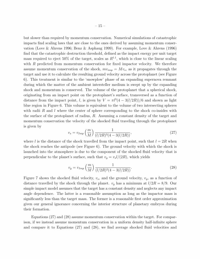
but slower than required by momentum conservation. Numerical simulations of catastrophic
impacts find scaling laws that are close to the ones derived by assuming momentum conser-
vation (Love & Ahrens 1996; Benz & Asphaug 1999). For example, Love & Ahrens (1996)
find that the catastrophic destruction threshold, defined as the impact energy per unit target
mass required to eject 50% of the target, scales as R1.1, which is close to the linear scaling
with R predicted from momentum conservation for fixed impactor velocity. We therefore
assume momentum conservation of the shock, mvimp = Mvs, as it propagates through the
target and use it to calculate the resulting ground velocity across the protoplanet (see Figure
6). This treatment is similar to the ‘snowplow’ phase of an expanding supernova remnant
during which the matter of the ambient intersteller medium is swept up by the expanding
shock and momentum is conserved. The volume of the protoplanet that a spherical shock,
originating from an impact point on the protoplanet’s surface, transversed as a function of
distance from the impact point, l, is given by V = πl3(4 − 3(l/2R))/6 and shown as light
blue region in Figure 6. This volume is equivalent to the volume of two intersecting spheres
with radii R and l where the center of sphere corresponding to the shock co-insides with
the surface of the protoplanet of radius, R. Assuming a constant density of the target and
momentum conservation the velocity of the shocked fluid traveling through the protoplanet
is given by
vs = vImp
(mM
) 1
(l/2R)3(4− 3(l/2R)), (27)
where l is the distance of the shock travelled from the impact point, such that l = 2R when
the shock reaches the antipode (see Figure 6). The ground velocity with which the shock is
launched into the atmosphere is due to the component of the shocked fluid velocity that is
perpendicular to the planet’s surface, such that vg = vsl/(2R), which yields
vg = vImp
(mM
) 1
(l/2R)2(4− 3(l/2R)). (28)
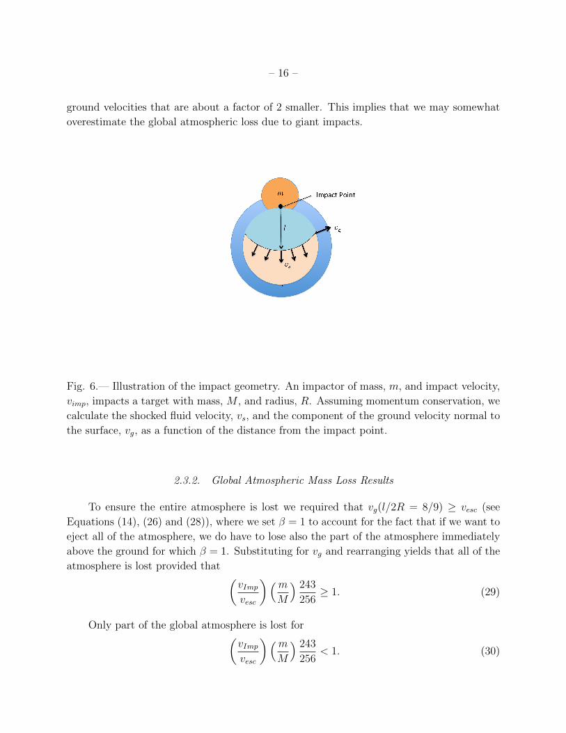
Figure 7 shows the shocked fluid velocity, vs, and the ground velocity, vg, as a function of
distance travelled by the shock through the planet. vg has a minimum at l/2R = 8/9. Our
simple impact model assumes that the target has a constant density and neglects any impact
angle dependence. The latter is a reasonable assumption as long as the impactor mass is
significantly less than the target mass. The former is a reasonable first order approximation
given our general ignorance concerning the interior structure of planetary embryos during
their formation.
Equations (27) and (28) assume momentum conservation within the target. For compar-
ison, if we instead assume momentum conservation in a uniform density half-infinite sphere
and compare it to Equations (27) and (28), we find average shocked fluid velocities and
– 16 –
ground velocities that are about a factor of 2 smaller. This implies that we may somewhat
overestimate the global atmospheric loss due to giant impacts.
Fig. 6.— Illustration of the impact geometry. An impactor of mass, m, and impact velocity,
vimp, impacts a target with mass, M , and radius, R. Assuming momentum conservation, we
calculate the shocked fluid velocity, vs, and the component of the ground velocity normal to
the surface, vg, as a function of the distance from the impact point.
2.3.2. Global Atmospheric Mass Loss Results
To ensure the entire atmosphere is lost we required that vg(l/2R = 8/9) ≥ vesc (see
Equations (14), (26) and (28)), where we set β = 1 to account for the fact that if we want to
eject all of the atmosphere, we do have to lose also the part of the atmosphere immediately
above the ground for which β = 1. Substituting for vg and rearranging yields that all of the
atmosphere is lost provided that (vImpvesc
)(mM
) 243
256≥ 1. (29)
Only part of the global atmosphere is lost for(vImpvesc
)(mM
) 243
256< 1. (30)
– 17 –
0.0 0.2 0.4 0.6 0.8 1.0
1
2
5
10
20
50
100
l�2R
Hv�v
ImpLH
M�mL
vg
vs
Fig. 7.— Shocked fluid velocity vs and the ground velocity vg as a function of distance
travelled by the shock, l, from the impact point to the other side of the planet, l = 2R.
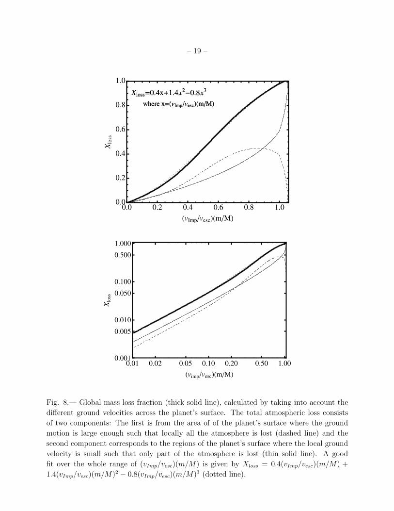
The atmospheric mass loss as a function of (vImp/vesc)(m/M) is shown in Figure 8. When
only a fraction of the atmosphere is lost, it is interesting to note that the total atmospheric
loss consists of two components: The first is from the area of the planet’s surface where the
ground motion is large enough such that locally all the atmosphere is lost (dashed line in
Figure 8), the second component corresponds to the region of the planet where the local
ground velocity is small enough such that only part of the atmosphere is lost (thin solid line
in Figure 8). In the latter case, the local fractional mass loss is given by Equation (14) for
an isothermal and Equation (26) for an adiabatic atmosphere, respectively.
In the limit that (vImp/vesc)(m/M)� 1, Equation (28) simplifies to vesc = vImp(m/4M)(2R/l)2
such that in the limit of small total atmospheric mass loss we have
Xloss =
(l
2R
)2
'( m
4M
)(vImpvesc
). (31)
In addition to the regions undergoing total atmospheric loss, we also have a contribution form
parts of the planet undergoing partial loss, yielding a total atmospheric mass loss fraction
Xloss = 0.4(m/M)(vImp/vesc). We note here that this formalism is less accurate for small
impactor masses with vImp ∼ vesc, since it does not include any atmosphere ejected directly
at the impact site (see Section 3).
– 18 –
More generally, we find that the global mass loss fraction for an isothermal atmosphere
is, independent of the exact value of the adiabatic index, well approximated by
Xloss = 0.4
(vImpm
vescM
)+ 1.4
(vImpm
vescM
)2
− 0.8
(vImpm
vescM
)3
(32)
and is plotted as dotted line, which is barely distinguishable from the thick solid line, in
Figure 8.
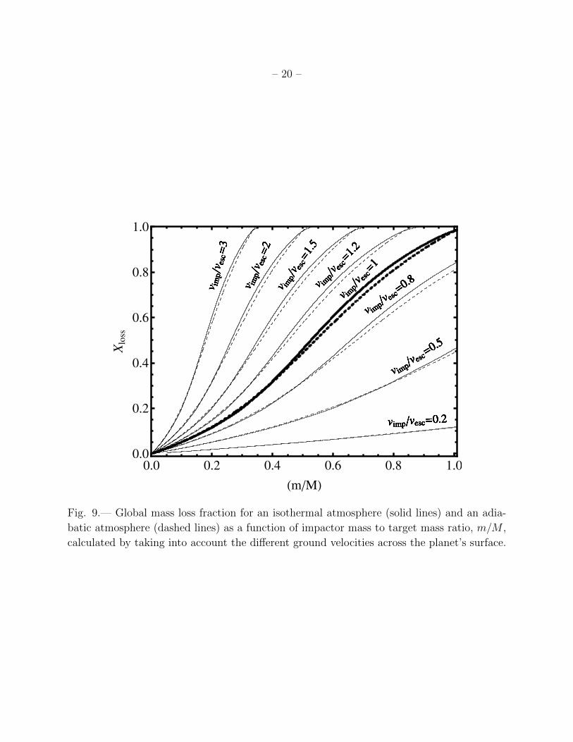
Similarly, for an adiabatic atmosphere we find
Xloss = 0.4
(vImpm
vescM
)+ 1.8
(vImpm
vescM
)2
− 1.2
(vImpm
vescM
)3
. (33)
Figure 9 shows the total atmospheric mass loss fraction for an isothermal (solid lines)
and adiabatic atmosphere (dotted line) as a function of impactor to target mass ratio for
various impact velocities. For a Mars-sized impactor hitting an 0.9 M⊕ protoplanet with
vImp ∼ vesc, we find Xloss = 6%. This is about a factor of 2 lower than estimates by Genda
& Abe (2003) who assumed an average ground velocity of 4 − 5 km/s across the whole
protoplanet and used this velocity together with their local atmospheric mass loss results
(similar to the ones shown in Figure 5) to estimate a global atmospheric mass loss of 10%.
We show here, however, that the global atmospheric mass loss consists of two components,
where the first component is from parts of the planet where the ground motion is large
enough such that locally all the atmosphere is lost (dashed line in Figure 8) and the second
component corresponds to the region of the planet where the local ground velocity is small
enough such that only part of the atmosphere is lost (thin solid line in Figure 8). This makes
the average ground velocity inadequate for determining the global atmospheric mass loss.
In the atmospheric mass loss calculations presented in this section, we assume that ratio
of specific heats, γ, is constant throughout the flow. However, the temperatures reached
during the shock propagation are high enough to lead to ionization of the atmosphere, which
in turn will decrease the value of γ and consequently result in reduced atmospheric mass
loss. The atmospheric mass loss due to giant impacts calculated in this section is therefore
an overestimate.
3. Atmospheric Mass Loss Due to Planetesimal Accretion and the Late Veneer
Although smaller impactors cannot individually eject a large fraction of the planetary
atmosphere, they collectively can play an important role in atmospheric erosion and, as we
show in section 4, may easily dominate atmospheric mass loss during planet formation.
– 19 –
0.0 0.2 0.4 0.6 0.8 1.00.0
0.2
0.4
0.6
0.8
1.0
HvImp�vescLHm�ML
Xlo
ss
Xloss=0.4x+1.4x2-0.8x
3
where x=HvImp�vescLHm�ML
Xloss=0.4x+1.4x2-0.8x
3
where x=HvImp�vescLHm�ML
0.01 0.02 0.05 0.10 0.20 0.50 1.000.001
0.005
0.010
0.050
0.100
0.500
1.000
Hvimp�vescLHm�ML
Xlo
ss
Fig. 8.— Global mass loss fraction (thick solid line), calculated by taking into account the
different ground velocities across the planet’s surface. The total atmospheric loss consists
of two components: The first is from the area of of the planet’s surface where the ground
motion is large enough such that locally all the atmosphere is lost (dashed line) and the
second component corresponds to the regions of the planet’s surface where the local ground
velocity is small such that only part of the atmosphere is lost (thin solid line). A good
fit over the whole range of (vImp/vesc)(m/M) is given by Xloss = 0.4(vImp/vesc)(m/M) +
1.4(vImp/vesc)(m/M)2 − 0.8(vImp/vesc)(m/M)3 (dotted line).
– 20 –
0.0 0.2 0.4 0.6 0.8 1.00.0
0.2
0.4
0.6
0.8
1.0
Hm�ML
Xlo
ss
vimp�vesc=0.2
v imp�v esc=
0.5
v imp�v es
c=
0.8
v imp�v
esc=1
v imp�v
esc=1.
2
v imp�v
esc=
1.5
v imp�v
esc=
2
vim
p�v
esc=
3
vimp�vesc=0.2
v imp�v esc=
0.5
v imp�v es
c=
0.8
v imp�v
esc=1
v imp�v
esc=1.
2
v imp�v
esc=
1.5
v imp�v
esc=
2
vim
p�v
esc=
3
vimp�vesc=0.2
v imp�v esc=
0.5
v imp�v es
c=
0.8
v imp�v
esc=1
v imp�v
esc=1.
2
v imp�v
esc=
1.5
v imp�v
esc=
2
vim
p�v
esc=
3
vimp�vesc=0.2
v imp�v esc=
0.5
v imp�v es
c=
0.8
v imp�v
esc=1
v imp�v
esc=1.
2
v imp�v
esc=
1.5
v imp�v
esc=
2
vim
p�v
esc=
3
vimp�vesc=0.2
v imp�v esc=
0.5
v imp�v es
c=
0.8
v imp�v
esc=1
v imp�v
esc=1.
2
v imp�v
esc=
1.5
v imp�v
esc=
2
vim
p�v
esc=
3
vimp�vesc=0.2
v imp�v esc=
0.5
v imp�v es
c=
0.8
v imp�v
esc=1
v imp�v
esc=1.
2
v imp�v
esc=
1.5
v imp�v
esc=
2
vim
p�v
esc=
3
vimp�vesc=0.2
v imp�v esc=
0.5
v imp�v es
c=
0.8
v imp�v
esc=1
v imp�v
esc=1.
2
v imp�v
esc=
1.5
v imp�v
esc=
2
vim
p�v
esc=
3
vimp�vesc=0.2
v imp�v esc=
0.5
v imp�v es
c=
0.8
v imp�v
esc=1
v imp�v
esc=1.
2
v imp�v
esc=
1.5
v imp�v
esc=
2
vim
p�v
esc=
3
Fig. 9.— Global mass loss fraction for an isothermal atmosphere (solid lines) and an adia-
batic atmosphere (dashed lines) as a function of impactor mass to target mass ratio, m/M ,
calculated by taking into account the different ground velocities across the planet’s surface.
– 21 –
3.1. Planetesimal Impacts
Unlike giant impacts which can create a strong shock propagating through the plane-
tary interior that in turn can launch a strong shock into the planetary atmosphere, smaller
planetesimal collisions can only eject the atmosphere locally. When a high-velocity impactor
hits the surface of the protoplanet, its velocity is sharply decelerated and its kinetic energy
is rapidly converted into heat and pressure resulting in something analogous to an explosion
(Zel’dovich & Raizer 1967). Similar to Vickery & Melosh (1990), we model the impact as
a point explosion on the surface, where a mass equal to the mass of the impactor, mImp,
propagates isotropically into a half-sphere with velocity of order, vesc. Atmosphere is ejected
only where its mass per unit solid angle, as measured from the impact point, is less than
that of the ejecta, mImp/2π. We can then relate the impactor mass, mImp, to the ejected
atmospheric mass Meject (see following Equations (34), (36) and (39)). These two masses
are not equal because the planetesimal impact launches a point-like isotropic explosion into
a half-sphere on the planetary surface, but the atmospheric mass above the tangent plane is
not isotropically distributed around the impact site (see Figure 10), but is more concentrated
towards the horizon. Specifically, the atmospheric mass close to the tangent plane of the
impact site is hardest to eject due to its larger column density.
In order to distinguish between the impactor mass and the mass ejected from the at-
mosphere we use M for the mass in the atmosphere that is ejected and, as in section 2, m
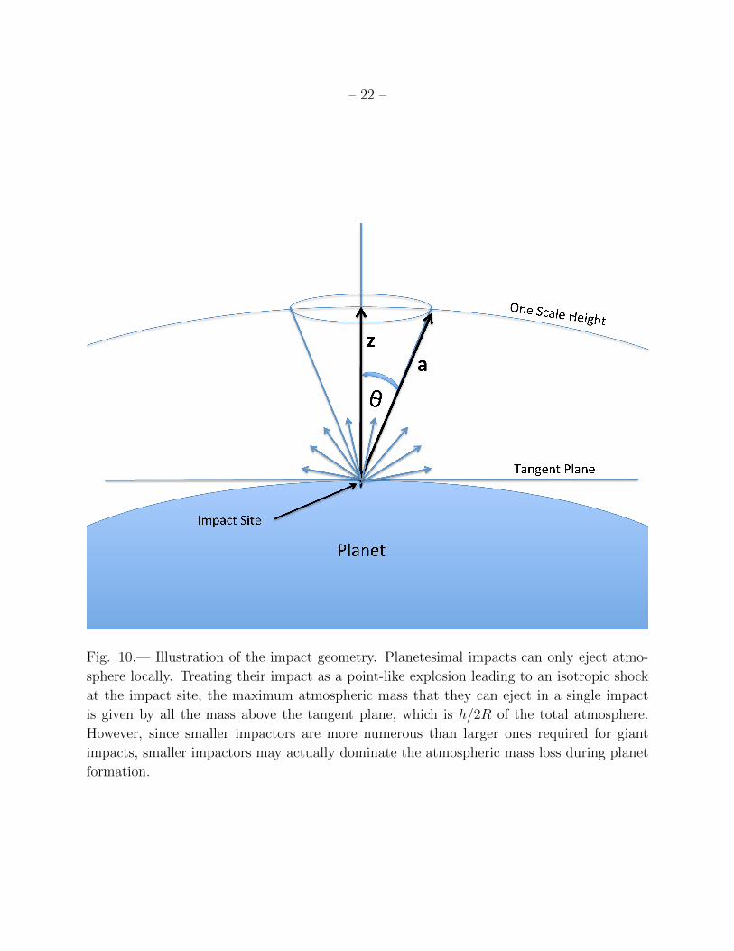
and r to describe the mass and radius of the impactor. Assuming an isothermal atmosphere,
which is a good approximation for the current Earth, the atmospheric mass inside a cone
defined by angle θ measured from the normal of the impact site (see Figure 10) is given by
MEject,θ = 2πρ0
∫ a=∞
a=0
∫ θ′=θ
θ′=0
exp[−z/h] sin θ′a2dθ′da (34)
where ρ0 is the atmospheric density at the surface of the planet and z is the height in the
atmosphere above the ground and is related to a, the distance from the impact site to the
top of the atmosphere (see Figure 10), by z = (a2 + 2aR cos θ′)/2R. Integrating over the
whole cap, i.e. from θ = 0 to θ = π/2, yields a total cap mass of
Mcap = 2πρ0h2R, (35)
in the limit that R � h, which applies for the terrestrial planets. This is the maximum
atmospheric mass that a single planetesimal impact can eject and is given by all the mass
above the tangent plane of the impact site. The ratio of the mass in the cap compared to
the total atmospheric mass is thereforeMcap/Matmos = h/2R. Atmospheric loss is therefore
limited to at best h/2R of the total atmosphere.
– 22 –
Fig. 10.— Illustration of the impact geometry. Planetesimal impacts can only eject atmo-
sphere locally. Treating their impact as a point-like explosion leading to an isotropic shock
at the impact site, the maximum atmospheric mass that they can eject in a single impact
is given by all the mass above the tangent plane, which is h/2R of the total atmosphere.
However, since smaller impactors are more numerous than larger ones required for giant
impacts, smaller impactors may actually dominate the atmospheric mass loss during planet
formation.
– 23 –
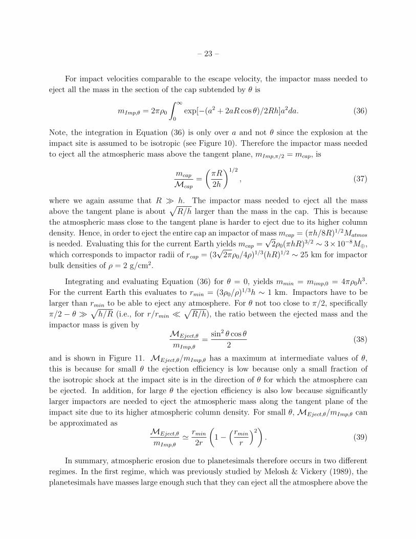
For impact velocities comparable to the escape velocity, the impactor mass needed to
eject all the mass in the section of the cap subtended by θ is
mImp,θ = 2πρ0
∫ ∞0
exp[−(a2 + 2aR cos θ)/2Rh]a2da. (36)
Note, the integration in Equation (36) is only over a and not θ since the explosion at the
impact site is assumed to be isotropic (see Figure 10). Therefore the impactor mass needed
to eject all the atmospheric mass above the tangent plane, mImp,π/2 = mcap, is
mcap
Mcap
=
(πR
2h
)1/2
, (37)
where we again assume that R � h. The impactor mass needed to eject all the mass
above the tangent plane is about√R/h larger than the mass in the cap. This is because
the atmospheric mass close to the tangent plane is harder to eject due to its higher column
density. Hence, in order to eject the entire cap an impactor of mass mcap = (πh/8R)1/2Matmos
is needed. Evaluating this for the current Earth yields mcap =√
2ρ0(πhR)3/2 ∼ 3×10⁻⁸M⊕,
which corresponds to impactor radii of rcap = (3√
2πρ0/4ρ)1/3(hR)1/2 ∼ 25 km for impactor
bulk densities of ρ = 2 g/cm2.
Integrating and evaluating Equation (36) for θ = 0, yields mmin = mimp,0 = 4πρ0h3.
For the current Earth this evaluates to rmin = (3ρ0/ρ)1/3h ∼ 1 km. Impactors have to be
larger than rmin to be able to eject any atmosphere. For θ not too close to π/2, specifically
π/2 − θ �√h/R (i.e., for r/rmin �
√R/h), the ratio between the ejected mass and the
impactor mass is given byMEject,θ
mImp,θ
=sin2 θ cos θ
2(38)
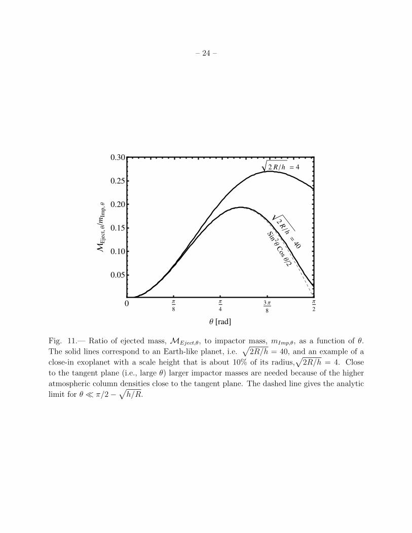
and is shown in Figure 11. MEject,θ/mImp,θ has a maximum at intermediate values of θ,
this is because for small θ the ejection efficiency is low because only a small fraction of
the isotropic shock at the impact site is in the direction of θ for which the atmosphere can
be ejected. In addition, for large θ the ejection efficiency is also low because significantly
larger impactors are needed to eject the atmospheric mass along the tangent plane of the
impact site due to its higher atmospheric column density. For small θ, MEject,θ/mImp,θ can
be approximated asMEject,θ
mImp,θ
' rmin2r
(1−
(rminr
)2). (39)
In summary, atmospheric erosion due to planetesimals therefore occurs in two different
regimes. In the first regime, which was previously studied by Melosh & Vickery (1989), the
planetesimals have masses large enough such that they can eject all the atmosphere above the
– 24 –
0 Π
8
Π
43 Π
8
Π
2
0.05
0.10
0.15
0.20
0.25
0.30
Θ @radD
ME
ject
,Θ�m
Imp,Θ
Sin 2Θ
Cos�2
2 R �h = 4
2R�h=
40
Fig. 11.— Ratio of ejected mass, MEject,θ, to impactor mass, mImp,θ, as a function of θ.
The solid lines correspond to an Earth-like planet, i.e.√
2R/h = 40, and an example of a
close-in exoplanet with a scale height that is about 10% of its radius,√
2R/h = 4. Close
to the tangent plane (i.e., large θ) larger impactor masses are needed because of the higher
atmospheric column densities close to the tangent plane. The dashed line gives the analytic
limit for θ � π/2−√h/R.
– 25 –
tangent plane, in this case the planetesimal masses must satisfy m ≥ mcap =√
2ρ0(πhR)3/2.
In the second regime, planetesimal impacts can only eject a fraction of the atmosphere above
the tangent plane and their masses must satisfy 4πρ0h3 < m <
√2ρ0(πhR)3/2. As we discuss
in section 5 and show in Figure 16, these small planetesimals are the most efficient impactors
(per unit mass) for removing planetary atmospheres and may actually dominate the mass
loss. Planetesimals with masses less than mmin = mimp,0 = 4πρ0h3 do not contribute to the
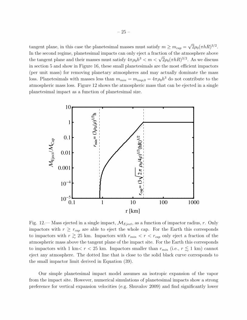
atmospheric mass loss. Figure 12 shows the atmospheric mass that can be ejected in a single
planetesimal impact as a function of planetesimal size.
0.1 1 10 100 100010-5
10-4
0.001
0.01
0.1
1
10
r @kmD
ME
ject�M
Cap
rm
in=H3Ρ
0�ΡL1�3
h
rca
p=H3
2ΠΡ
0�4ΡL1�3Hh
RL1�2
rm
in=H3Ρ
0�ΡL1�3
h
rca
p=H3
2ΠΡ
0�4ΡL1�3Hh
RL1�2
Fig. 12.— Mass ejected in a single impact,MEject, as a function of impactor radius, r. Only
impactors with r ≥ rcap are able to eject the whole cap. For the Earth this corresponds
to impactors with r & 25 km. Impactors with rmin < r < rcap only eject a fraction of the
atmospheric mass above the tangent plane of the impact site. For the Earth this corresponds
to impactors with 1 km< r < 25 km. Impactors smaller than rmin (i.e., r . 1 km) cannot
eject any atmosphere. The dotted line that is close to the solid black curve corresponds to
the small impactor limit derived in Equation (39).
Our simple planetesimal impact model assumes an isotropic expansion of the vapor
from the impact site. However, numerical simulations of planetesimal impacts show a strong
preference for vertical expansion velocities (e.g. Shuvalov 2009) and find significantly lower
– 26 –
atmospheric mass loss for vertical impacts (Svetsov 2007) compared to oblique ones (Shuvalov
2009). In contrast, in oblique impacts, the plume expands more isotropically and hence
accelerates and ejects more atmospheric mass (Shuvalov 2009). Comparing the results of
our simple planetesimal impact model with the numerical results, averaged over all impact
angles, obtained by Shuvalov (2009)1, we find that we overestimateMEject/mImp by a factor
of 10, 3 and 1 for impact velocities of 15 km/s, 20 km/s and 30 km/s, respectively. In deriving
Equation (36), we assume that impact velocities comparable to vesc are sufficient to result in a
point like explosion, where a mass equal to the mass of the impactor propagates isotropically
with velocity of order vesc, but comparison with numerical impact simulations above suggests
that impactor velocities of about 3vesc are needed to produce such an explosion. We did
not investigate the dependence of MEject/mImp on the impact velocity. Previous works of
numerical impact simulations find that bigger impact velocities lead to larger atmospheric
mass loss, smaller values for rmin and r∗ (Svetsov 2007; Shuvalov 2009). From Equation (39)
we find thatMEject/mImp has a maximum at r∗ =√
3rmin, which corresponds to about 2 km
for the current Earth. This compares well the values of r∗ found by Shuvalov (2009) which
are 2 km, 1 km, and 1 km for impact velocities of 15 km/s, 20 km/s and 30 km/s, respectively.
Finally, the scaling ofMEject/mImp shown in Figure 3 of Shuvalov (2009) is consistent with
the MEject/mImp ∝ m−1/3Imp scaling we find from Equation (39) for r∗ < r < rcap and the
MEject/mImp ∝ m−1Imp scaling we find for rcap < r (see also Figure 16).
3.2. Impactor Size Distributions
Similar to Melosh & Vickery (1989), we can now calculate the atmospheric mass loss
rate due to planetesimal impacts for a given impactor flux. Parameterizing the cumulative
impactor flux with a single power law given by N(> r) = N0(r/r0)−q+1, where q is the
differential power law index, N0 is the impactor flux (number per unit time per unit area)
normalized to impactors with radii r0, we can write the atmospheric mass loss rate as
dMatmos
dt= −πR2N0(q − 1)
r0
∫ rmax
rmin
(r
r0
)−qMEject(r)dr. (40)
1The dimensionless erosional efficiency given in Equation (2) of Shuvalov (2009) seems to contain a typo,
since in its printed form it is not dimensionless. When comparing our results with Shuvalov (2009) we
assume that the author intended to have ρ2 in denominator rather than just ρ, where ρ is the density of the
impactor.
– 27 –
If the planetesimal size distribution is dominated by the smallest bodies such that q > 3
thendMatmos
dt= −πR2N0(q − 1)mmin
2r0
∫ rmax
rmin
(r
r0
)−q((r
rmin
)2
− 1
)dr (41)
where we substituted for Meject from Equation (39). Integrating over r gives
dMatmos
dt= −πR2N0mmin
q − 3
(rminr0
)−q+1
(42)
where rmin = (3ρ0/ρ)1/3h and mmin = 4πρ0h3. Evaluating Equation (42) for q = 4 yields
dMatmos/dt = −πR2N04π3ρr30.
If q < 3 then the atmospheric mass loss is dominated by impactors whose mass is around
the smallest mass that can eject the entire cap. For this case we find for 3 > q > 1
dMatmos
dt= −πR2CN0Mcap
(rcapr0
)−q+1
, (43)
where rcap = (3√
2πρ0/4ρ)1/3(hR)1/2 is the impactor radius that can eject all the atmosphere
above the tangent plane andMcap = 2πρ0h2R is the mass of the atmosphere above the tan-
gent plane. C is a constant that accounts for the additional contribution to the atmospheric
mass loss from bodies that can only eject a fraction of the atmosphere above the tangent
plane. C = 1 implies that bodies smaller than rcap do not contribute to the atmospheric
mass loss for 3 > q > 1. The numerical value of C depends on the impactor size distribution
because it is the bodies that are just a little bit smaller than rcap that can still contribute
significantly to the atmospheric mass loss. We find that the values for C range from 2.8 for
q = 2.8, 1.9 for q = 2.5, 1.3 for q = 2.0, to 1.1 for q = 1.5. As expected, the value of C is
largest for q close to 3 because the larger q, the more numerous are the smaller bodies.
The time it takes to lose the entire atmosphere is finite, i.e. the mass in the atmosphere
does not simply decline exponentially towards zero but reaches zero in a finite time (Melosh
& Vickery 1989). This is because as some of the atmosphere is lost, its density declines and
even smaller impactors can now contribute to the atmospheric mass loss. This accelerates
the mass loss process, because smaller impactors are more numerous and dominate the mass
loss (see Equations (42) and (43)). From Equations (42) and (43) we find that for both q > 3
and 1 < q < 3 impactor size distributions that the rate of atmospheric mass loss scales as
Matmos/dt ∝ −M (−q+4)/3atmos and has a solution given by
Matmos(t) = M0
(1− t
t∗
)3/(q−1)
, (44)
– 28 –
where M0 is the initial atmospheric mass at t = 0 and t∗ is the time it takes to lose the entire
atmosphere. Interestingly the solutions to Equation (44) for both q > 3 and 1 < q < 3 only
differ by the value of t∗. For 1 < q < 3
t∗q<3 =6
π(q − 1)CRhN0
(√πh
8R
M0
m0
)(q−1)/3
(45)
and for q > 3 the time for complete atmospheric loss is
t∗q>3 =3(q − 3)
π(q − 1)h2N0
((h
R
)2M0
m0
)(q−1)/3
, (46)
where m0 = 4πρr30/3 and r0 is the radius to which the size distribution is normalized. The
expression in Equation (45) differs from the one derived by Melosh & Vickery (1989) because
they assumed Mcap = mcap, whereas we find that Mcap = mcap(2h/πR)1/2 (see Equation
(37)), and they neglected the numerical coefficient C.
4. Comparison of Atmospheric Mass Loss due to Giant Impacts and
Planetesimal Accretion
Having derived the atmospheric mass loss due to giant impacts and smaller planetesimal
impacts, we are now in the position to compare these different mass loss regimes.
Assuming that all impactors have the same size, we find for rmin < r < rcap that the
number of impactors needed to remove the atmosphere is
N =Matmos
MEject
= 6ρ0h
ρrmin
(R
r
)2(1−
(rminr
)2)−1(47)
and that this corresponds to a total mass in impactors given by
MT =MatmosmImp
MEject
=2r
rmin
(1−
(rminr
)2)−1Matmos. (48)
Strictly speaking the Equations (47) and (48) overestimate N and MT , because as a fraction
of the remaining atmosphere is removed a given sized impactor is able to eject a larger
fraction of the atmosphere above the tangent plane. In deriving Equations (47) and (48) we
used Equation (39) for the relationship between the ejected mass and the impactor mass,
which is only valid for r/rmin �√R/h. Equations (47) and (48) are therefore not accurate
for r ∼ rcap but should still give a reasonable estimate for Earth-like atmospheres since the
– 29 –
deviation between the approximation and full solution is small and only occurs in the vicinity
around r ∼ rcap (see Figure 12).
Similarly, for impactors large enough to remove the entire cap but not too large to be
in the giant impact regime (i.e., rcap < r < rgi), we have
N =Matmos
MEject
=2R
h(49)
and
MT =MatmosmImp
MEject
=4π
3ρr3
2R
h. (50)
In contrast to the previous regime, rmin < r < rcap, impactors with rcap < r < rgi are
always limited to ejecting the whole cap, so an impactor of a given size cannot eject more
atmosphere as the total atmospheric mass declines with time.
We estimate the impactor radius at which giant impacts are more efficient than smaller
impacts in ejecting the atmosphere, by equating the atmospheric mass loss due to giant
impacts to the atmospheric cap mass. Assuming that vImp ∼ vesc, we find by equating
Equation (31) to the fraction of the atmosphere above the tangent plane that rgi ' (2hR2)1/3,
which corresponds to impactors with radii of about 900 km for the current Earth. Finally,
from Equation (31) we have that in the giant impact regime (i.e., r > rgi)
N =Matmos
MEject
= X−1loss '3R3
r3(51)
and
MT =MatmosmImp
MEject
' 4M = constant. (52)
Equations (51) and (52) were derived in the limit that Xloss � 1 in a single giant impact.
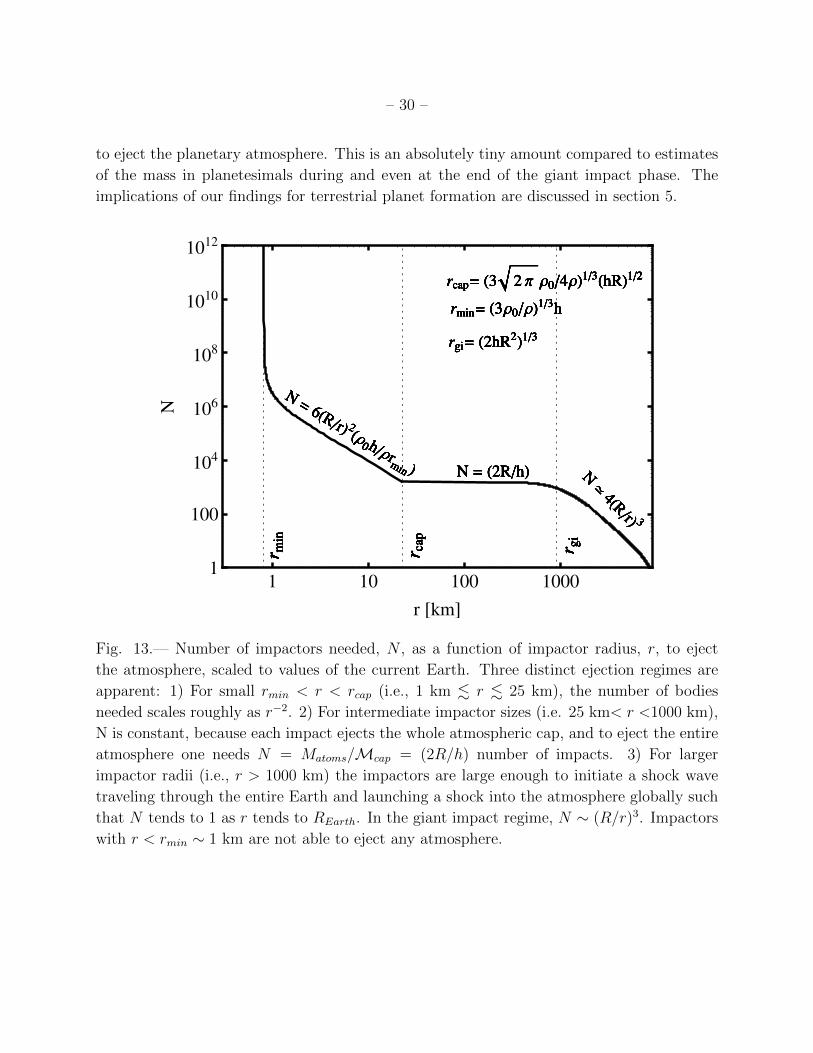
Figure 13 shows the number of impactors needed, defined here as N = Matoms/MEject,
to erode the atmosphere as a function of impactor radius. Figure 14 shows the total mass in
impactors needed, defined here as MT = MatomsmImp/MEject, to erode the atmosphere as a
function of impactor radius. Figure 15 is the same as Figure 14 but for atmospheric mass
that is 100 times enhanced compared to that of the current Earth. The plots in all three
figures assume that all impactors are identical and have a single size, r. Figures 13, 14 and
15 clearly display the three distinct ejection regimes. Figures 14 and 15 impressively show
that small impactors with rmin < r < rcap are the most effective impactors per unit mass in
ejecting the atmosphere. The best impactor size for atmospheric mass loss is r∗ =√
3rminfor which mImp/MEject = 33/2 ' 5. For the current Earth this corresponds to bodies with
r ∼ 2 km and implies that a total mass in such impactors only needs to be about 5Matoms
– 30 –
to eject the planetary atmosphere. This is an absolutely tiny amount compared to estimates
of the mass in planetesimals during and even at the end of the giant impact phase. The
implications of our findings for terrestrial planet formation are discussed in section 5.
1 10 100 10001
100
104
106
108
1010
1012
r @kmD
N
rmin= H3Ρ0�ΡL1�3h
rcap= H3 2 Π Ρ0�4ΡL1�3HhRL1�2
rgi= H2hR2L1�3
N>
4HR�rL 3
N=
6HR�rL 2HΡ
0 h�Ρrmin L N = H2R�hL
rm
in
rca
p
rgi
rmin= H3Ρ0�ΡL1�3h
rcap= H3 2 Π Ρ0�4ΡL1�3HhRL1�2
rgi= H2hR2L1�3
N>
4HR�rL 3
N=
6HR�rL 2HΡ
0 h�Ρrmin L N = H2R�hL
rm
in
rca
p
rgi
rmin= H3Ρ0�ΡL1�3h
rcap= H3 2 Π Ρ0�4ΡL1�3HhRL1�2
rgi= H2hR2L1�3
N>
4HR�rL 3
N=
6HR�rL 2HΡ
0 h�Ρrmin L N = H2R�hL
rm
in
rca
p
rgi
rmin= H3Ρ0�ΡL1�3h
rcap= H3 2 Π Ρ0�4ΡL1�3HhRL1�2
rgi= H2hR2L1�3
N>
4HR�rL 3
N=
6HR�rL 2HΡ
0 h�Ρrmin L N = H2R�hL
rm
in
rca
p
rgi
rmin= H3Ρ0�ΡL1�3h
rcap= H3 2 Π Ρ0�4ΡL1�3HhRL1�2
rgi= H2hR2L1�3
N>
4HR�rL 3
N=
6HR�rL 2HΡ
0 h�Ρrmin L N = H2R�hL
rm
in
rca
p
rgi
rmin= H3Ρ0�ΡL1�3h
rcap= H3 2 Π Ρ0�4ΡL1�3HhRL1�2
rgi= H2hR2L1�3
N>
4HR�rL 3
N=
6HR�rL 2HΡ
0 h�Ρrmin L N = H2R�hL
rm
in
rca
p
rgi
rmin= H3Ρ0�ΡL1�3h
rcap= H3 2 Π Ρ0�4ΡL1�3HhRL1�2
rgi= H2hR2L1�3
N>
4HR�rL 3
N=
6HR�rL 2HΡ
0 h�Ρrmin L N = H2R�hL
rm
in
rca
p
rgi
Fig. 13.— Number of impactors needed, N , as a function of impactor radius, r, to eject
the atmosphere, scaled to values of the current Earth. Three distinct ejection regimes are
apparent: 1) For small rmin < r < rcap (i.e., 1 km . r . 25 km), the number of bodies
needed scales roughly as r−2. 2) For intermediate impactor sizes (i.e. 25 km< r <1000 km),
N is constant, because each impact ejects the whole atmospheric cap, and to eject the entire
atmosphere one needs N = Matoms/Mcap = (2R/h) number of impacts. 3) For larger
impactor radii (i.e., r > 1000 km) the impactors are large enough to initiate a shock wave
traveling through the entire Earth and launching a shock into the atmosphere globally such
that N tends to 1 as r tends to REarth. In the giant impact regime, N ∼ (R/r)3. Impactors
with r < rmin ∼ 1 km are not able to eject any atmosphere.
– 31 –
1 10 100 1000
1.´ 10-6
0.0001
0.01
1
r @kmD
MT�MÅ
Matmos�MÅ
Mocean�MÅ
rm
in
rca
pMT�Mŵ
r
MT�Mŵ
r3
MT�Mŵ const
rgi
Matmos�MÅ
Mocean�MÅ
rm
in
rca
pMT�Mŵ
r
MT�Mŵ
r3
MT�Mŵ const
rgi
Matmos�MÅ
Mocean�MÅ
rm
in
rca
pMT�Mŵ
r
MT�Mŵ
r3
MT�Mŵ const
rgi
Matmos�MÅ
Mocean�MÅ
rm
in
rca
pMT�Mŵ
r
MT�Mŵ
r3
MT�Mŵ const
rgi
Matmos�MÅ
Mocean�MÅ
rm
in
rca
pMT�Mŵ
r
MT�Mŵ
r3
MT�Mŵ const
rgi
Matmos�MÅ
Mocean�MÅ
rm
in
rca
pMT�Mŵ
r
MT�Mŵ
r3
MT�Mŵ const
rgi
Matmos�MÅ
Mocean�MÅ
rm
in
rca
pMT�Mŵ
r
MT�Mŵ
r3
MT�Mŵ const
rgi
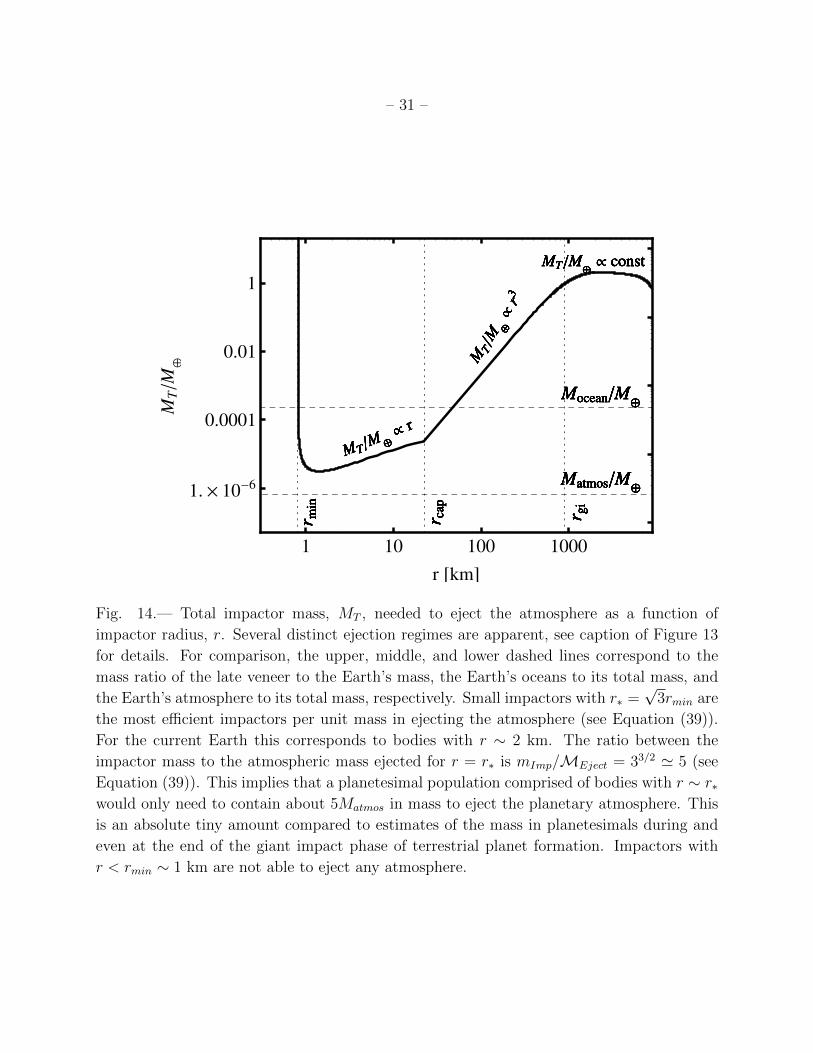
Fig. 14.— Total impactor mass, MT , needed to eject the atmosphere as a function of
impactor radius, r. Several distinct ejection regimes are apparent, see caption of Figure 13
for details. For comparison, the upper, middle, and lower dashed lines correspond to the
mass ratio of the late veneer to the Earth’s mass, the Earth’s oceans to its total mass, and
the Earth’s atmosphere to its total mass, respectively. Small impactors with r∗ =√
3rmin are
the most efficient impactors per unit mass in ejecting the atmosphere (see Equation (39)).
For the current Earth this corresponds to bodies with r ∼ 2 km. The ratio between the
impactor mass to the atmospheric mass ejected for r = r∗ is mImp/MEject = 33/2 ' 5 (see
Equation (39)). This implies that a planetesimal population comprised of bodies with r ∼ r∗would only need to contain about 5Matmos in mass to eject the planetary atmosphere. This
is an absolute tiny amount compared to estimates of the mass in planetesimals during and
even at the end of the giant impact phase of terrestrial planet formation. Impactors with
r < rmin ∼ 1 km are not able to eject any atmosphere.
– 32 –
1 10 100 1000
1.´ 10-6
0.0001
0.01
1
r @kmD
MT�MÅ
100Matmos�MÅ
Late Veneer
rm
in
rca
p
MT�Mŵ r
MT�Mŵ
r3
MT�Mŵ const
rgi
100Matmos�MÅ
Late Veneer
rm
in
rca
p
MT�Mŵ r
MT�Mŵ
r3
MT�Mŵ const
rgi
100Matmos�MÅ
Late Veneer
rm
in
rca
p
MT�Mŵ r
MT�Mŵ
r3
MT�Mŵ const
rgi
100Matmos�MÅ
Late Veneer
rm
in
rca
p
MT�Mŵ r
MT�Mŵ
r3
MT�Mŵ const
rgi
100Matmos�MÅ
Late Veneer
rm
in
rca
p
MT�Mŵ r
MT�Mŵ
r3
MT�Mŵ const
rgi
100Matmos�MÅ
Late Veneer
rm
in
rca
p
MT�Mŵ r
MT�Mŵ
r3
MT�Mŵ const
rgi
100Matmos�MÅ
Late Veneer
rm
in
rca
p
MT�Mŵ r
MT�Mŵ
r3
MT�Mŵ const
rgi
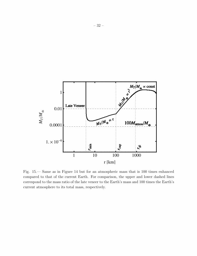
Fig. 15.— Same as in Figure 14 but for an atmospheric mass that is 100 times enhanced
compared to that of the current Earth. For comparison, the upper and lower dashed lines
correspond to the mass ratio of the late veneer to the Earth’s mass and 100 times the Earth’s
current atmosphere to its total mass, respectively.
– 33 –
5. Application & Importance for the Formation of the Terrestrial Planets
Earth, Venus and Mars all display similar geochemical abundance patterns of near
chondritic light noble gasses, but relative depletion of in Xe, C and N (e.g. Halliday 2013).
This suggests that all three planets may not only have lost major volatiles, but also accreted
similar veneers from chondritic material. In addition, all three planets have similar noble
gas patterns, but whereas the budgets for Venus are near chondritic, the budgets for Earth
and Mars are depleted by two and four orders of magnitude, respectively. This suggests that
Earth and Mars lost the vast majority of their noble gasses relative to Venus during the
process of planet formation (Halliday 2013).
Recent work suggests that the Earth went through at least two separate periods during
which its atmosphere was lost (Tucker & Mukhopadhyay 2014). The evidence for several
atmospheric loss events is inferred from the mantle 3He/22Ne, which is higher than the
primordial solar abundance by at least a factor of 6 and which is thought to have been
increased to its current value by multiple magma ocean degassing episodes and atmospheric
loss events. In addition, Tucker & Mukhopadhyay (2014) suggest that the preservation of low3He/22Ne ratio in a primitive reservoir sampled by plumes implies that later giant impacts
did not generate a global magma ocean.
Previous works usually appeal to giant impacts to explain Earth’s atmospheric mass
loss episodes (e.g. Genda & Abe 2003, 2005). Figure 14, however, demonstrates clearly that
small planetesimals with sizes rmin < r < rcap are the most efficient impactors per unit
mass in ejecting the atmosphere. For the current Earth this corresponds to bodies with
1km . r . 25 km. Furthermore, atmospheric mass loss due to small impactors will proceed
without generating a global magma ocean, which is supported by recent interpretations of
low 3He/22Ne ratios in a primitive reservoir sampled by plumes (Tucker & Mukhopadhyay
2014).
Whether or not planetesimal impacts will lead to a net loss of planetary atmospheres or
simply an alteration of the current atmosphere depends on the planetesimal sizes distribution
as well as the volatile content of the planetesimals. Zahnle et al. (1992) investigated impact
erosion and replenishment of planetary atmospheres and suggest that the competition of
these two processes can explain the present distributions of atmospheres between Ganymede,
Callisto, and Titan. de Niem et al. (2012) performed a similar study with a focus on Earth
and Mars during a heavy bombardment and find a dominance of accumulation over erosion.
Figure 16 shows the ratio of atmospheric mass ejected to impactor mass as a function of
planetesimal size. If the impactors are not dominated by a single size, as assumed in Figure
16, but instead follow a power-law size distribution, N(> r) = N0(r/r0)−q+1, then the ratio
– 34 –
of the atmospheric mass lost to the impactor mass is, for 3 < q < 4, given by
dMatmos
dmImp
= − 4− q(q − 1)(q − 3)
(rminrmax
)−q+4
+ f, (53)
where rmax is the maximum size of the planetesimal size distribution and rmin = (3ρ0/ρ)1/3h
is the smallest planetesimal size that can contribute to the atmospheric mass loss as derived
in section 2 and f is the volatile fraction of the planetesimals. Similarly, for 1 < q < 3 we
havedMatmos
dmImp
= −C(
2h
πR
)1/24− qq − 1
(rcaprmax
)−q+4
+ f, (54)
where rcap = (3√
2πρ0/4ρ)1/3(hR)1/2 and corresponds to the impactor radius that can eject
all the atmospheric mass above the tangent plane. Evaluating the first term in Equations
(53) and (54) for a planetesimal population ranging from r < rmin ∼ 1 km to 1000 km
and assuming values of the current Earth we find dMatmos/dmImp = −0.01 + f for q = 3.5
and dMatmos/dmImp = −0.0003 + f for q = 2.5, respectively 2. These results have two
important implications: First, we can estimate how massive initial planetary atmospheres
must have been in order to avoid erosion due to planetesimal impacts. Estimates of the mass
in planetesimals during the giant impact phase range from a few percent to several tens of
percent of the total mass in terrestrial planets (e.g. Schlichting et al. 2012). Assuming a total
mass in planetesimals of about 0.1 M⊕ yields that initial atmospheres must have contained
Matmos & 10−3M⊕ and Matmos & 3×10⁻⁵M⊕ for q = 3.5 and q = 2.5, respectively, in order to
avoid erosion due to planetesimal impacts. The latter result is particular interesting since it
implies that for q = 2.5 Venus, which has Matmos ∼ 8×10⁻⁵M⊕, will not undergo atmospheric
erosion due to planetesimal impacts whereas the Earth could have lost most of its atmosphere
due to planetesimal impacts if its initial atmosphere was less than 3 × 10⁻⁵M⊕. Second,
Equations (53) and (54) permit an equilibrium solution, where the atmospheric erosion is
balanced by the volatiles delivered to the planet’s atmosphere in a given planetesimal impact.
It may therefore be that the Earth’s atmosphere was eroded by planetesimal impacts until an
equilibrium was established between atmospheric loss and volatile gain. The current Earth’s
atmosphere could be the result of such an equilibrium if the fraction of the planetesimal
mass that ends up as volatiles in the atmosphere, f , was 0.01 and 3× 10⁻⁴ for q = 3.5 and
q = 2.5, respectively. These finding are consistent with results by de Niem et al. (2012) who
find that atmospheric erosion is balanced by volatile delivery from an asteroidal population
of impactors if f = 2× 10⁻³.
2For comparison, the lunar craters can be modeled with a power-law size distribution with q ∼ 2.8 and
q ∼ 3.2 for crater diameters ranging from 1 km to 64 km and larger than 64 km, respectively (e.g. Neukum
et al. 2001).
– 35 –
1 10 100 100010-6
10-5
10-4
0.001
0.01
0.1
1
r @kmD
ME
ject�m
Imp
rm
in=H3Ρ
0�ΡL1�3
h
rca
p=H3
2ΠΡ
0�4ΡL1�3Hh
RL1�2
Earth Rock
Lunar Rock
Carbonaceous Chondritesr
min=H3Ρ
0�ΡL1�3
h
rca
p=H3
2ΠΡ
0�4ΡL1�3Hh
RL1�2
Earth Rock
Lunar Rock
Carbonaceous Chondritesr
min=H3Ρ
0�ΡL1�3
h
rca
p=H3
2ΠΡ
0�4ΡL1�3Hh
RL1�2
Earth Rock
Lunar Rock
Carbonaceous Chondritesr
min=H3Ρ
0�ΡL1�3
h
rca
p=H3
2ΠΡ
0�4ΡL1�3Hh
RL1�2
Earth Rock
Lunar Rock
Carbonaceous Chondrites
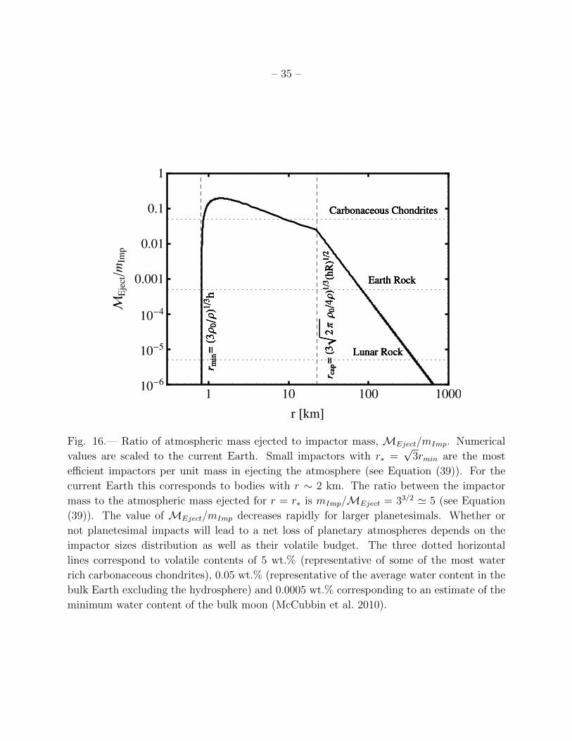
Fig. 16.— Ratio of atmospheric mass ejected to impactor mass, MEject/mImp. Numerical
values are scaled to the current Earth. Small impactors with r∗ =√
3rmin are the most
efficient impactors per unit mass in ejecting the atmosphere (see Equation (39)). For the
current Earth this corresponds to bodies with r ∼ 2 km. The ratio between the impactor
mass to the atmospheric mass ejected for r = r∗ is mImp/MEject = 33/2 ' 5 (see Equation
(39)). The value of MEject/mImp decreases rapidly for larger planetesimals. Whether or
not planetesimal impacts will lead to a net loss of planetary atmospheres depends on the
impactor sizes distribution as well as their volatile budget. The three dotted horizontal
lines correspond to volatile contents of 5 wt.% (representative of some of the most water
rich carbonaceous chondrites), 0.05 wt.% (representative of the average water content in the
bulk Earth excluding the hydrosphere) and 0.0005 wt.% corresponding to an estimate of the
minimum water content of the bulk moon (McCubbin et al. 2010).
– 36 –
To summarize, we have shown that planetesimals can be very efficient in atmospheric
erosion and that the amount of atmospheric loss depends on the total mass in planetesimals,
on their size distribution and their volatile content. The total planetesimal mass needed for
significant atmospheric loss is small and it is therefore likely that planetesimal impacts played
a major role in atmospheric mass loss over the formation history of the terrestrial planets.
We have shown that the current differences in Earth’s and Venus’ atmospheric masses can
be explained by modest differences in their initial atmospheric masses and that the current
atmosphere of the Earth could have resulted from an equilibrium between atmospheric ero-
sion and volatile delivery to the atmosphere by planetesimal impacts. Furthermore, if the
Earth’s hydrosphere was dissolved in its atmosphere, as it may have been immediately after
a giant impact, then planetesimal impacts can also have contributed significantly to loss of
the Earth’s oceans. We have shown above that planetesimals can be very efficient in atmo-
spheric erosion and that the amount of atmospheric loss depends both on the total mass in
planetesimals, on their size distribution and their volatile content. One way for planetesimals
to not participate significantly in the atmospheric erosion of some, or all, of the terrestrial
planets is for most of their mass to reside in bodies smaller than rmin = (3ρ0/ρ)1/3h, since
such bodies are too small to contribute to atmospheric loss. Finally, planetesimal impacts
may not only have played a major role in atmospheric erosion of the terrestrial planets but
may also have contributed significantly to the current terrestrial planet atmospheres.
6. Discussion & Conclusions
We investigated the atmospheric mass loss during planet formation and found that it
can proceed in three different regimes.
1) In the first regime (r & rgi = (2hR2)1/3), giant impacts create strong shocks that
propagate through the planetary interior causing a global ground motion of the protoplanet.
This ground motion in turn launches a strong shock into the planetary atmosphere, which
can lead to loss of a significant fraction or even the entire atmosphere. We find that the local
atmospheric mass loss fraction due to giant impacts for ground velocities vg . 0.25vesc is
given by χloss = (βvg/vesc)p where β and p are constants equal to β = 1.71, p=4.9 (isothermal
atmosphere and an adiabatic index γ = 5/3) and β = 2.11, p=7.6 (adiabatic atmosphere
with polytropic index n = 1.5, adiabatic index γ = 5/3). In addition, using a simple model
of a spherical shock propagating through the target, we find that the global atmospheric
mass loss fraction is well characterized by Xloss ' 0.4x + 1.2x2 − 0.8x3 (isothermal) and
Xloss ' 0.4x + 1.8x2 − 1.2x3 (adiabatic), where x = (vImpm/vescM), independent of the
precise value of the adiabatic index.
– 37 –
2) In the second regime (rcap = (3√
2πρ0/4ρ)1/3(hR)1/2 . r . (2hR2)1/3 = rgi), im-
pactors cannot eject the atmosphere globally, but are large enough, i.e., r > rcap, to eject all
the atmosphere above the tangent plane of the impact site. A single impactor is therefore
limited to ejecting h/2R of the total atmosphere in a given impact. For the current Earth
this corresponds to impactor sizes satisfying 25 km . r . 900 km.
3) In the third regime (rmin = (3ρ0/ρ)1/3h . r . (3√
2πρ0/4ρ)1/3(hR)1/2 = rcap),
impactors are only able to eject a fraction of the atmospheric mass above the tangent plane
of the impact site. For the current Earth this corresponds to 1 km . r . 25 km. Impactors
with r . rmin are not able to eject any atmosphere.
Comparing these three atmospheric mass loss regimes, we find that the most efficient
impactors (per unit impactor mass) for atmospheric loss are small planetesimals. For the
current atmosphere of the Earth this corresponds to impactor radii of about 2 km. For such
impactors, the ejected mass to impactor mass ratio is only ∼ 5, implying that one only
needs about 5 times the total atmospheric mass in such small impactors to active complete
loss. More realistically, planetesimal sizes were probably not constrained to a single size,
but spanned by a range of sizes. For impactor flux size distributions parametrized by a
power law, N > r ∝ r−q+1, with differential power law index q we find that for 1 < q < 3 the
atmospheric mass loss is dominated by bodies that eject all the atmosphere above the tangent
plane (r > rcap) and that for q > 3 the mass loss is dominated by impactors that only erode a
fraction of the atmospheric mass above the tangent plane in a single impact (rmin < r < rcap).
Assuming that the planetesimal population ranged in size from r < rmin ∼ 1 km to 1000 km,
we find for, parameters corresponding to the current Earth, an atmospheric mass loss rate
to impactor mass rate ratio of 0.01 and 0.0003 for q = 3.5 and q = 2.5, respectively. Despite
being bombarded by the same planetesimal population, we find that the current differences
in Earth’s and Venus’ atmospheric masses can be explained by modest differences in their
initial atmospheric masses and that the current atmosphere of the Earth could have resulted
from an equilibrium between atmospheric erosion and volatile delivery to the atmosphere
from planetesimal impacts.
Recent work suggests that the Earth went through at least two separate periods dur-
ing which its atmosphere was lost and that later giant impacts did not generate a global
magma ocean (Tucker & Mukhopadhyay 2014). Such a scenario is challenging to explain
if atmospheric mass loss was a byproduct of giant impacts, because a combination of large
impactor masses and large impact velocities is needed to achieve complete atmospheric loss
(see Figure 8). Furthermore, giant impacts that could accomplish complete atmospheric loss,
almost certainly will generate a global magma ocean. Since atmospheric mass loss due to
small planetesimal impacts will proceeded without generating a global magma ocean they
– 38 –
offer a solution to this conundrum.
To conclude, we have shown that planetesimals can be very efficient in atmospheric
erosion and that the amount of atmospheric loss depends on the total mass in planetesimals,
on their size distribution and their volatile content. The total planetesimal mass needed
for significant atmospheric loss is small and it is therefore likely that planetesimal impacts
played a major role in the atmospheric mass loss history of the Earth and during planet
formation in general. In addition, small planetesimal impacts may also have contributed
significantly to the current terrestrial planet atmospheres.
Acknowledgements: We thank H. J. Melosh and the second anonymous referee for
their constructive reviews and D. Jewitt, T. Grove, N. Inamdar for helpful comments and
suggestions. RS dedicates this paper to the late Tom Ahrens, who initiated his interest in
the problem of atmospheric escape and collaborated on related ideas.
REFERENCES
Agnor, C. B., Canup, R. M., & Levison, H. F. 1999, Icarus, 142, 219
Ahrens, T. J. 1993, Annual Review of Earth and Planetary Sciences, 21, 525
Benz, W., & Asphaug, E. 1999, Icarus, 142, 5. arXiv:astro-ph/9907117
Chambers, J. E. 2001, Icarus, 152, 205
Chevalier, R. A. 1990, ApJ, 359, 463
de Niem, D., Kuhrt, E., Morbidelli, A., & Motschmann, U. 2012, Icarus, 221, 495
Genda, H., & Abe, Y. 2003, Icarus, 164, 149
— 2005, Nature, 433, 842
Goldreich, P., Lithwick, Y., & Sari, R. 2004, ApJ, 614, 497. astro-ph/0404240
Grover, R., & Hardy, J. W. 1966, ApJ, 143, 48
Halliday, A. N. 2013, Geochim. Cosmochim. Acta, 105, 146
Ida, S., & Makino, J. 1993, Icarus, 106, 210
Kenyon, S. J., & Bromley, B. C. 2006, AJ, 131, 1837. astro-ph/0503568
– 39 –
Kompaneets, A. S. 1960, Soviet Physics Doklads English Translation, 5, 46
Love, S. G., & Ahrens, T. J. 1996, Icarus, 124, 141
McCubbin, F. M., Steele, A., Hauri, E. H., Nekvasil, H., Yamashita, S., & Hemley, R. J.
2010, Proceedings of the National Academy of Science, 107, 11223
Melosh, H. J., & Vickery, A. M. 1989, Nature, 338, 487
Neukum, G., Ivanov, B. A., & Hartmann, W. K. 2001, Space Sci. Rev., 96, 55
Newman, W. I., Symbalisty, E. M. D., Ahrens, T. J., & Jones, E. M. 1999, Icarus, 138, 224
Raizer, Y. P. 1964, Zh. Prikl. Mekham. i Tekhn. Fiz., 4, 49
Schlichting, H. E., Warren, P. H., & Yin, Q.-Z. 2012, ApJ, 752, 8. 1202.6372
Shuvalov, V. 2009, Meteoritics and Planetary Science, 44, 1095
Svetsov, V. V. 2007, Solar System Research, 41, 28
Tucker, J. M., & Mukhopadhyay, S. 2014, ArXiv e-prints. 1403.0806
Vickery, A. M., & Melosh, H. J. 1990, Geological Society of America, 247, 289
Walker, R. J. 2009, Chemie der Erde / Geochemistry, 69, 101
Walker, R. J., Horan, M. F., Shearer, C. K., & Papike, J. J. 2004, Earth and Planetary
Science Letters, 224, 399
Warren, P. H., Kallemeyn, G. W., & Kyte, F. T. 1999, Geochim. Cosmochim. Acta, 63, 2105
Weidenschilling, S. J., Spaute, D., Davis, D. R., Marzari, F., & Ohtsuki, K. 1997, Icarus,
128, 429
Zahnle, K., Kasting, J. F., & Pollack, J. B. 1990, Icarus, 84, 502
Zahnle, K., Pollack, J. B., Grinspoon, D., & Dones, L. 1992, Icarus, 95, 1
Zel’dovich, Y. B., & Raizer, Y. P. 1967, Physics of shock waves and high-temperature hy-
drodynamic phenomena
This preprint was prepared with the AAS LATEX macros v5.2.