Adv. Geosci., 35, 105–113, 2013www.adv-geosci.net/35/105/2013/doi:10.5194/adgeo-35-105-2013© Author(s) 2013. CC Attribution 3.0 License.

EGU Journal Logos (RGB)

Advances in Geosciences

Open A

ccess

Natural Hazards and Earth System

Sciences

Open A

ccess

Annales Geophysicae

Open A

ccess

Nonlinear Processes in Geophysics

Open A

ccess

Atmospheric Chemistry

and Physics

Open A

ccess

Atmospheric Chemistry

and Physics

Open A

ccess

Discussions

Atmospheric Measurement

Techniques

Open A

ccess

Atmospheric Measurement

Techniques

Open A

ccess

Discussions

Biogeosciences

Open A

ccess

Open A

ccess

BiogeosciencesDiscussions

Climate of the Past

Open A

ccess

Open A

ccess

Climate of the Past

Discussions

Earth System Dynamics

Open A

ccess

Open A

ccess

Earth System Dynamics

Discussions

GeoscientificInstrumentation

Methods andData Systems

Open A

ccess

GeoscientificInstrumentation

Methods andData Systems

Open A

ccess

Discussions

GeoscientificModel Development

Open A

ccess

Open A

ccess

GeoscientificModel Development

Discussions

Hydrology and Earth System

Sciences

Open A

ccess

Hydrology and Earth System

Sciences

Open A

ccess

Discussions

Ocean Science

Open A

ccess

Open A

ccess

Ocean ScienceDiscussions

Solid Earth

Open A

ccess

Open A

ccess

Solid EarthDiscussions

The Cryosphere

Open A

ccess

Open A

ccess

The CryosphereDiscussions

Natural Hazards and Earth System

Sciences

Open A

ccess

DiscussionsAtmospheric corrections in interferometric synthetic aperture radarsurface deformation – a case study of the city of Mendoza, Argentina

S. Balbarani1, P. A. Euillades1, L. D. Euillades1, F. Casu2, and N. C. Riveros1

1CEDIAC Institute, National University of Cuyo, 5500 Mendoza, Argentina2IREA Institute, National Research Council, 80124 Naples, Italy

Correspondence to:S. Balbarani (sbalbarani@cediac.uncu.edu.ar)

Received: 5 February 2013 – Revised: 25 July 2013 – Accepted: 26 July 2013 – Published: 4 September 2013

Abstract. Differential interferometry is a remote sensingtechnique that allows studying crustal deformation producedby several phenomena like earthquakes, landslides, land sub-sidence and volcanic eruptions. Advanced techniques, likesmall baseline subsets (SBAS), exploit series of images ac-quired by synthetic aperture radar (SAR) sensors during agiven time span.

Phase propagation delay in the atmosphere is the mainsystematic error of interferometric SAR measurements. It af-fects differently images acquired at different days or even atdifferent hours of the same day. So, datasets acquired duringthe same time span from different sensors (or sensor con-figuration) often give diverging results. Here we processedtwo datasets acquired from June 2010 to December 2011 byCOSMO-SkyMed satellites. One of them is HH-polarized,and the other one is VV-polarized and acquired on differentdays.

As expected, time series computed from these datasetsshow differences. We attributed them to non-compensated at-mospheric artifacts and tried to correct them by using ERA-Interim global atmospheric model (GAM) data. With thismethod, we were able to correct less than 50 % of the scenes,considering an area where no phase unwrapping errors weredetected. We conclude that GAM-based corrections are notenough for explaining differences in computed time series,at least in the processed area of interest. We remark that nodirect meteorological data for the GAM-based correctionswere employed. Further research is needed in order to under-stand under what conditions this kind of data can be used.

1 Introduction

Differential synthetic aperture radar interferometry (DIn-SAR) is an advanced remote sensing technique aimed tolarge-scale surface deformations monitoring with centime-ter to millimeter accuracy, by exploiting the round-trip phasecomponents of SAR images relative to an investigated area(Massonnet and Feigl, 1998). Information of ground defor-mation is associated with the phase difference between twoacquisitions, referred to as master and slave images of theinterferometric data pair. Both acquisitions must be acquiredfrom relatively close tracks (spatial baseline) and acquisitiontime (temporal baseline) in order to reduce the temporal andgeometric decorrelation phenomena and topographic errors(Berardino et al., 2002).

An effective way for studying and understanding the dy-namics of the deformation phenomena and their temporal be-havior is the generation of deformation time series. Multi-temporal InSAR techniques were developed recently; theyare based on combining information obtained from multi-ple SAR images acquired over a period of time. The mostwidely used advanced DInSAR algorithms are small base-line subsets (SBAS) approach (Berardino et al., 2002) andpersistent scatterer (PS) (Ferretti et al., 2001). SBAS tech-nique is based on an adequate combination of the differentialinterferograms characterized by a small spatial and temporalseparation (spatial and temporal baseline) in order to limitthe geometric and temporal decorrelation phenomena and tomaximize the number of coherent pixels exploited. Its capa-bility of detecting and investigating long-time deformationphenomena has been already shown in different applicationsbased on exploiting ERS and ENVISAT data of the EuropeanSpace Agency (ESA) (Pepe et al., 2005; Tizzani et al., 2007).

Published by Copernicus Publications on behalf of the European Geosciences Union.

106 S. Balbarani et al.: Atmospheric corrections in interferometric synthetic aperture radar surface deformation

Fig. 1. Distribution of HH and VV data acquisitions. Most of the acquisitions were alternately selected in HH and VV polarization mode in8 days.

Furthermore, deformation time-series generation capabilityof the small baseline subset algorithm to the Radarsat-1 datahas been demonstrated (Euillades et al., 2009).

Phase propagation delay in the atmosphere is the mainsystematic error of interferometric SAR measurements. Thedominant contribution of the atmospheric phase delay, whichmay reach tens of centimeters, comes from the temporalvariation of the stratified troposphere (Hanssen, 2001). Suchvariations are related to changes in variables such us tem-perature, atmospheric pressure and water vapor. In particu-lar, atmospheric water vapor effects represent one of the ma-jor limitations for repeat-pass InSAR, and limit the accuracyof deformation rates derived from DInSAR (Li et al., 2006).Due to their dependence on altitude, such variations may pro-duce a spatial correlation between the magnitude of the phaseSAR signal and the topographic elevation.

Several methods have been recommended for estimatingatmospheric phase delay corrections and isolating displace-ments from atmospheric artifacts. For example, Onn and Ze-bker (2006) use zenithal wet delay observations from GPSNetwork. Li et al. (2006) employ satellite multispectral im-agery analysis, and Jolivet et al. (2011) profit from globalatmospheric model (GAM) derived data.

The atmospheric contribution becomes potentially greateras the SAR wavelength becomes shorter (Hanssen, 2001).This is an issue when processing data acquired by thenew generation X-band satellites like COSMO-SkyMed andTerraSAR-X. Conversely, crustal deformation monitoringcan benefit from the high spatial and temporal resolution ofthese sensors. Furthermore, the fact that several SAR sensorsare simultaneously orbiting Earth makes potentially avail-able series of scenes covering a given area during a commontime span. As systems are characterized by different polar-ization and/or acquisition geometry, and the scenes are even-tually not acquired on the same days/hours, the emergingquestion is if the area of interest’s deformation history canbe accurately characterized by using DInSAR-based tech-niques. In other words, are time series computed from scenesacquired at different times with different systems or withthe same system but different polarization giving the sameresults? As the underlying deformation is the same, even-tual differences could be attributed to not well-compensated

atmospheric contributions and/or processing (phase unwrap-ping) errors.

In this work we present the results of an experiment con-sistent in computing deformation time series by exploitingHH- and VV-polarized SAR data acquired during a commontime span by COSMO-SkyMed satellites. Covered area is astrip of roughly 40× 50 km located near the city of Men-doza in western Argentina. Obtained results show significantdifferences among the two elaborations, which motivate usto explore if estimating the atmospheric phase delay fromERA-Interim global atmospheric model (GAM) is useful asan operative correction tool.

2 Data and processing

2.1 Dataset and study area

We used two COSMO-SkyMed datasets composed of31 HH-polarized and 27 VV-polarized images respectively.Acquisition geometry is the same for all scenes: stripmapmode (HIMAGE), descending pass with an incidence angleof 38◦. Both datasets cover the period between June 2010and December 2011, but HH- and VV-polarized scenes wereacquired on different days, as can be seen in Fig. 1.

Different land uses are well represented within the selectedtest site: (1) urban areas (Mendoza city), (2) agricultural cov-erage around the city, (3) piedmont and bare soil with lowvegetation and (4) high relief (Andes Mountains). Area loca-tion and main characteristics are presented in Fig. 2.

2.2 A brief description of the SBAS algorithm

This brief description is based on Berardino et al. (2002).Consideringn + 1 SAR images relative to the same area, ac-quired at chronological ordered time [t0, t1, . . . tn] and as-suming that all the images are co-registered, the DInSAR-SBAS algorithm begins with an adequate combination of im-age pairs, which allows minimizing geometrical and tempo-ral decorrelation. A numberm of multilook differential in-terferograms are generated. Unwrapped differential phase ofthek-th interferogram, considered at the generic pixel of az-imuth and range coordinates (x, r), is expressed by

Adv. Geosci., 35, 105–113, 2013 www.adv-geosci.net/35/105/2013/

S. Balbarani et al.: Atmospheric corrections in interferometric synthetic aperture radar surface deformation 107

Fig. 2. Study area: the city of Mendoza, Argentina.(A) The yel-low box identifies an approximation of the orbital descending foot-print of HH and VV COSMO-SkyMed dataset. Background image:Landsat-8 sensor of 23 May 2013 (path: 232, row: 83). Source:http://landsatlook.usgs.gov/. (B) The city of Mendoza is located inMendoza Province, in central-western Argentina.

δϕk(x, r) = ϕ (x, r, tB) − ϕ (x, r, tA)

≈4π

λ[d(x, r, tB) − d(x, r, tA)]

+1ϕtopok (x, r) + 1ϕatm

k (x, r, tA, tB) + 1nk(x, r), (1)

wherek = 1, . . . ,m; tA and tB are the acquisition times ofmaster and slave images and

1ϕtopok (x, r) ≈

4π

λ

B⊥,k 1z(x, r)

r sinϑ. (2)

ϕ(x, r, tB) − ϕ(x, r, tA) represents the phases of the twoimages involved in the interferogram generation,λ is theradar wavelength, d(x, r, tA) and d(x, r, tB) are the radarline-of-sight (LOS) projections of the cumulative surface de-formation at the two timestA and tB . 1ϕ

topok (x, r) takes

into account possible topographic artifacts1z(x, r) thatcan be present in the digital elevation model (DEM) usedfor topographic phase component compensation. The term1ϕatm

k (x, r, tA, tB ) accomplishes possible atmospheric dis-turbances between the acquisitions at timestA and tB , and

it is often referred to as a atmospheric phase component.1nk(x, r) accounts for the noise effects. Finally,B⊥,k repre-sents the perpendicular baseline component andϑ the SARsensor look angle.

Considering phase velocities between adjacent acquisi-tions, Eqs. (1) and (2) allow defining a system of equationsin then + 1 unknowns:

vT=

[v1 =

ϕ1

t1 − t0, . . . , vn =

ϕn − ϕn−1

tn − tn−1, 1z

]. (3)

This can be solved by using the single value decomposition(SVD) asB v = δϕ in a matrix form.

As a result, the SBAS algorithm gives displacement timeseries for each processed pixel. Atmospheric artifacts are fil-tered through the application of low pass filtering step in thetwo-dimensional spatial domain followed by a temporal highpass filtering.

2.3 DInSAR-SBAS processing

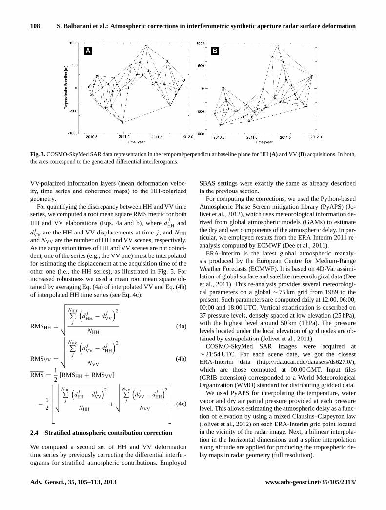
Both datasets were processed separately, and 85 HH and78 VV differential interferograms were computed accordingto the SBAS restrictions on temporal and spatial baselines.The maximum perpendicular baseline allowed was 1000 m,which is one-third of the critical baseline for the acquisi-tion geometry. However, the longest one effectively used was751 m (24 December 2010–25 January 2011) for HH elabo-ration and 923 m (23 April 2011–9 May 2011) for VV elabo-ration. The maximum temporal baseline was 150 days. Spa-tial vs. temporal baseline distribution is shown in Fig. 3,where scenes and interferograms are represented by pointsand arcs, respectively. The 30 m X-band SRTM DEM (Rabuset al., 2003) was used for the topographic phase removal. HHand VV time series were computed by inverting the interfer-ograms after phase unwrapping process with an extension ofthe minimum-cost flow (MCF) algorithm (Pepe and Lanari,2006). Finally, atmospheric contributions are filtered out byusing a set of filters in cascade as described in Tizzani etal. (2007).

Mean deformation velocity maps, computed from bothelaborations, are shown in Fig. 4 (SAR projection, azimuthin the horizontal direction) where low coherent pixels havebeen masked out. Time series are referred to a pixel (RP –reference point) located in Mendoza city (white triangle inFig. 4), considered “stable” or point of zero deformation. Weconsidered unreliable those pixels with temporal coherence(Tizzani et al., 2007) lower than 0.8. As expected, coherentpixel density is higher in urban and piedmont areas than inagricultural or high relief ones.

Obtained deformation sequences were co-registered forcomparing the results. To do so we computed the azimuth andrange shifts of the VV-polarized elaboration master scene(6 March 2011) with respect to the HH-polarized master one(25 January 2011) by using a 2048× 2048 pixel window.Those shifts were subsequently used for accommodating the

www.adv-geosci.net/35/105/2013/ Adv. Geosci., 35, 105–113, 2013

108 S. Balbarani et al.: Atmospheric corrections in interferometric synthetic aperture radar surface deformation

Fig. 3.COSMO-SkyMed SAR data representation in the temporal/perpendicular baseline plane for HH(A) and VV (B) acquisitions. In both,the arcs correspond to the generated differential interferograms.

VV-polarized information layers (mean deformation veloc-ity, time series and coherence maps) to the HH-polarizedgeometry.

For quantifying the discrepancy between HH and VV timeseries, we computed a root mean squareRMS metric for bothHH and VV elaborations (Eqs. 4a and b), whered

jHH and

djVV are the HH and VV displacements at timej , andNHH

andNVV are the number of HH and VV scenes, respectively.As the acquisition times of HH and VV scenes are not coinci-dent, one of the series (e.g., the VV one) must be interpolatedfor estimating the displacement at the acquisition time of theother one (i.e., the HH series), as illustrated in Fig. 5. Forincreased robustness we used a mean root mean square ob-tained by averaging Eq. (4a) of interpolated VV and Eq. (4b)of interpolated HH time series (see Eq. 4c):

RMSHH =

√√√√√√NHH∑

j

(d

jHH − d

jVV

)2

NHH(4a)

RMSVV =

√√√√√√NVV∑

j

(d

jVV − d

jHH

)2

NVV(4b)

RMS =1

2[RMSHH + RMSVV ]

=1

2

√√√√√√NHH∑

j

(d

jHH − d

jVV

)2

NHH+

√√√√√√NVV∑

j

(d

jVV − d

jHH

)2

NVV

. (4c)

2.4 Stratified atmospheric contribution correction

We computed a second set of HH and VV deformationtime series by previously correcting the differential interfer-ograms for stratified atmospheric contributions. Employed

SBAS settings were exactly the same as already describedin the previous section.

For computing the corrections, we used the Python-basedAtmospheric Phase Screen mitigation library (PyAPS) (Jo-livet et al., 2012), which uses meteorological information de-rived from global atmospheric models (GAMs) to estimatethe dry and wet components of the atmospheric delay. In par-ticular, we employed results from the ERA-Interim 2011 re-analysis computed by ECMWF (Dee et al., 2011).

ERA-Interim is the latest global atmospheric reanaly-sis produced by the European Centre for Medium-RangeWeather Forecasts (ECMWF). It is based on 4D-Var assimi-lation of global surface and satellite meteorological data (Deeet al., 2011). This re-analysis provides several meteorologi-cal parameters on a global∼ 75 km grid from 1989 to thepresent. Such parameters are computed daily at 12:00, 06:00,00:00 and 18:00 UTC. Vertical stratification is described on37 pressure levels, densely spaced at low elevation (25 hPa),with the highest level around 50 km (1 hPa). The pressurelevels located under the local elevation of grid nodes are ob-tained by extrapolation (Jolivet et al., 2011).

COSMO-SkyMed SAR images were acquired at∼ 21:54 UTC. For each scene date, we got the closestERA-Interim data (http://rda.ucar.edu/datasets/ds627.0/),which are those computed at 00:00 GMT. Input files(GRIB extension) corresponded to a World MeteorologicalOrganization (WMO) standard for distributing gridded data.

We used PyAPS for interpolating the temperature, watervapor and dry air partial pressure provided at each pressurelevel. This allows estimating the atmospheric delay as a func-tion of elevation by using a mixed Clausius–Clapeyron law(Jolivet et al., 2012) on each ERA-Interim grid point locatedin the vicinity of the radar image. Next, a bilinear interpola-tion in the horizontal dimensions and a spline interpolationalong altitude are applied for producing the tropospheric de-lay maps in radar geometry (full resolution).

Adv. Geosci., 35, 105–113, 2013 www.adv-geosci.net/35/105/2013/

S. Balbarani et al.: Atmospheric corrections in interferometric synthetic aperture radar surface deformation 109

Fig. 4. HH and VV mean deformation velocity maps superimposed on the amplitude images of the study area of the city of Mendoza. (RP)identifies the reference point of the start the unwrapping process.(A) and(C) represent a singular area in HH results, and(B) and(D) in VVresults. deformation time series:(A) and(B) near the Potrerillos Dam;(C) and(D) in the city of Mendoza.

High-resolution tropospheric delay maps were multi-looked to the COSMO-SkyMed scene processing resolution.Furthermore, we referenced them to the time of the first ac-quisition and to the reference point (RP). Subsequently, wegenerated the corrections for each one of the 2π -wrappeddifferential interferograms and applied them to the originalones.

In Fig. 6 we show an example of the computed atmo-spheric corrections for the differential interferogram com-posed by acquisitions 15 June 2010 (master) and 1 July 2010(slave). Note the topography-correlated fringes are indicatedby two arrows in Fig. 6a and the stratified delay maps pre-dicted by ERA-Interim in Fig. 6c. Finally note in Fig. 6dhow these signals were significantly reduced after correction,

www.adv-geosci.net/35/105/2013/ Adv. Geosci., 35, 105–113, 2013

110 S. Balbarani et al.: Atmospheric corrections in interferometric synthetic aperture radar surface deformation

Fig. 5. Example of deformation time series (DTS). White trianglerepresents HH displacement, asterisk VV deformation and black tri-angle VV DTS interpolated at HH series.

Fig. 6. Example of a COSMO-SkyMed interferogram and atmo-spheric correction over the area of interest using the ERA-I globalatmospheric model. All images are in radar geometry.(A) Wrappedinterferogram from SAR acquisitions on 15 June 2010 (master) and1 July 2010 (slave). Perpendicular baseline = 184 m., temporal base-line = 16 days.(B) Black dots: pixel phase values as a function of el-evation.(C) Corresponding stratified delay map predicted by ERA-Interim. (D) 2π -wrapped differential interferogram corrected fromthe topography-dependent atmospheric effects.

suggesting that they are due to topography-dependent watervapor effects.

The whole procedure employed for generating uncorrectedand corrected time series is summarized in the flow chart dis-played in Fig. 7.

Fig. 7. Flow chart of the procedure employed for generating uncor-rected and corrected deformation time series (DTS).

3 Results and discussion

Mean deformation velocity maps computed as described inSect. 2.2 are shown in Fig. 4. The maps show significant dif-ferences. Near the reference point RP, in the urban area ofMendoza city, the velocity is almost zero in both elabora-tions. As we move away from the RP, noticeable differencesin magnitude and sign of the LOS (line-of-sight) mean de-formation velocities can be observed. In general, deforma-tion velocity of the whole area, for the time span processed,is lower than 1.3 cm yr−1 in absolute value. However, local-scale subsidence patterns of about 2 cm yr−1 were detectedin both HH and VV elaborations (see Fig. 4) near PotrerillosDam (a and b), and in Mendoza city (c and d). VV elabora-tion reports velocities systematically higher than HH ones inthese areas.

As the mean deformation velocity gives only a quick lookof the underlying data, which are the deformation time se-ries, we based our analysis on them. We computed the aver-age RMS map by using Eq. (4c). An amplitude scene, DEM,and average RMS map are shown in Fig. 8A–C, respec-tively. From the figure, a correlation between RMS map andtopography is apparent: lower areas (around the Mendozacity) show RMS of 0 mm, which increases up to∼ 35 mm inhigher areas. One can detect roughly three areas of different

Adv. Geosci., 35, 105–113, 2013 www.adv-geosci.net/35/105/2013/

S. Balbarani et al.: Atmospheric corrections in interferometric synthetic aperture radar surface deformation 111

Fig. 8. Correlation between RMS map and topography:(A) amplitude of COSMO-SkyMed SAR image on 25 January 2011 (master).(B) Digital elevation model in radar geometry generated from X-Band SRTM (Shuttle Radar Topography Mission).(C) Average RMS map.(a)–(f) represent HH and VV deformation time series.

RMS ranges colored blue, green and red in Fig. 8C. Timeseries extracted at those RMS levels are also shown in thereferred figure: in Mendoza city area (i.e., blue RMS zone)(Fig. 8a) HH and VV series have similar behavior and lowRMS; in bare soil, agricultural area and near the Potreril-los Dam (i.e., the green RMS zone) (Fig. 8b–d), HH andVV series show good correlation except for a group ofscenes acquired between roughly 24 December 2010 and14 March 2011. Finally, HH and VV series are very noisy inthe mountainous area (red RMS zone) thus producing highvalues of RMS.

Correlation between average RMS and topography, andthe fact that high RMS values are due to differences be-tween time series at some dates (e.g., 24 December 2010 to14 March 2011), at least in the green RMS zone, motivatedus to hypothesize that differences in computed time seriesare related to non-compensated stratified tropospheric phasecomponents. In order to prove this idea, we corrected thedifferential interferograms and re-computed the deformationtime series with the procedure already described in Sect. 2.3.Obtained results are presented in Fig. 9, where RMS mapscomputed by Eqs. (4a) and (4b) for non-corrected-HH, -VVand corrected-HH, -VV time series are displayed. Clearly,RMSs for corrected time series are higher than RMSs fornon-corrected ones in areas topographically higher, whereasit diminishes in lower areas, particularly those located in the

near range: see highlighted box and time series A, B, C andD in the figure.

In order to understand why the time series, and conse-quently the RMS metric, are heavily affected in the moun-tainous region (see VV RMS map and E, F time series inFig. 9), we analyzed the unwrapping residuals. Unwrappingresiduals compute the difference between differential inter-ferograms and synthetic differential interferograms recon-structed from phase time series after SVD inversion (moredetails can be seen in Tizzani et al., 2007). If both interfer-ograms are equal, which means that phase unwrapping wascorrect, residuals are near zero. Sometimes non-zero resid-ual are found in relatively isolated areas in terms of co-herence, thus indicating non-reliable unwrapping there. Fig-ure 10 presents significant residual maps computed after theERA-Interim VV- and HH-corrected elaborations. Note thatnon-zero residuals are found in areas that correlate well withareas of RMS worsening. This could explain the observed ef-fect: high RMS is not necessarily the result of failed correc-tions but of processing errors in the phase unwrapping step.

At this point, it is interesting to check if the correlationbetween unwrapped phase and topography before and af-ter correction systematically diminished. For that compari-son we do not used the unwrapped interferograms but theunwrapped phase obtained after the SBAS inversion via sin-gle value decomposition. Note that the unwrapped phase map

www.adv-geosci.net/35/105/2013/ Adv. Geosci., 35, 105–113, 2013

112 S. Balbarani et al.: Atmospheric corrections in interferometric synthetic aperture radar surface deformation

Fig. 9.RMS maps for non-corrected-HH, -VV and corrected-HH, -VV time series.(A)–(F) represent HH and VV deformation time series.

relevant for each acquisition can be understood as a syntheticinterferogram computed between it and the first acquisition(in time) of the series. We computed the Pearson correlationcoefficient, which improved in 8 HH and 13 VV scenes af-ter correction, whereas it became worse in 23 HH and 14 VVscenes. If, instead of computing correlation in the whole area,we restrict it to near the range of low RMS zone (white boxin Fig. 9), the results are as follows: Pearson’s coefficient im-proved in 17 HH and 9 VV scenes after correction, whereasit become worse in 14 HH and 18 VV scenes. The correctionseems to work in the HH time series, but fails in the VV one.

In summary, many interferograms show topography corre-lated fringes, which are an indication of atmospheric strat-ification components in the differential phase. Correctionscomputed from ERA-Interim GAM remove the correlationbetween phase and topography in some scenes, but not in allof them. We also detected unwrapping errors affecting thehigh relief areas, so they should not be taken into account foratmospheric correction statistics. But inside the area withoutunwrapping errors, corrections perform well only in the HHelaboration. Possibly, corrections derived from a GAM in anarea without enough direct meteorological data do not accu-rately represent the atmospheric state. Errors could be also

derived from using GAM data computed for a time that dif-fers in a few hours from the SAR passing time.

4 Conclusions

We computed deformation time series from HH- and VV-polarized COSMO-SkyMed SAR images acquired during acommon time span. Algorithm used was DInSAR-SBAS.Results show noticeable differences between both elabora-tions, which is clearly a processing artifact given that the un-derlying deformation is the same. As scenes were acquiredon different days, we explore using atmospheric data for cor-recting them.

We detected correlation between unwrapped phase and to-pography in both elaborations. Furthermore, differences be-tween time series, quantified with a RMS metric, also showcorrelation with elevation: differences increase with height.

We applied corrections for stratified atmospheric com-ponents, computed by using independent data provided byERA-Interim GAM. From the obtained results, we concludethat they are not enough for minimizing difference betweenthe time series. In fact, the correction improves some of theinterferograms (by removing topography-correlated fringes)

Adv. Geosci., 35, 105–113, 2013 www.adv-geosci.net/35/105/2013/

S. Balbarani et al.: Atmospheric corrections in interferometric synthetic aperture radar surface deformation 113

Fig. 10.Phase unwrapping residual maps computed after the ERA-Interim VV and HH corrections. Interferograms:(A) 14 Novem-ber 2010 (master)–1 January 2011 (slave),(B) 16 October 2011(master)–1 November 2011 (slave),(C) 16 December 2010(master)–1 January 2011 (slave) and(D) 18 February 2011(master)–6 March 2011 (slave).

but worsens others (increasing the correlation). This couldsuggest that GAM models fail to represent accurately the at-mospheric state in this region, at least for some of the acqui-sition dates. Lack of direct meteorological data could explainthis behavior, but further work for verifying this hypothesisneeds to be done.

Acknowledgements.The authors thank the IREA-CNR (Naples,Italy) personnel for collaborating in COSMO-SkyMed data pro-cessing. Furthermore, we want to thank Piyush Shanker Agram ofthe Seismological Laboratory (CALTECH), for helpful suggestions.

Edited by: K. TokeshiReviewed by: two referees

References

Berardino, P., Fornaro, G., Lanari, R., and Sansosti, E.: A New Al-gorithm for Surface Deformation Monitoring Based on SmallBaseline Differential SAR Interferograms, IEEE T. Geosci. Re-mote, 40, 2375–2383, 2002

Dee, D. P., Uppala, S. M., Simmons, A. J., Berrisford, P., Poli, P.,Kobayashi, S., Andrae, U., Balmaseda, M. A., Balsamo, G., andBauer, P.: The ERA-Interim Reanalysis: Configuration and Per-formance of the Data Assimilation System, Q. J. Roy. Meteorol.Soc., 137, 553–597, 2011.

Euillades, L., Pepe, A., Berardino, P., Bonano, M., Sansosti, E.,and Lanari, R.: RADARSAT-1 Deformation Time-series Gener-ation by Using the SBAS-DInSAR Algorithm, in: Radar Con-ference, 2009 IEEE,http://ieeexplore.ieee.org/xpls/absall.jsp?arnumber=4977079, last access: 26 December 2012, 1–4, 2009.

Ferretti, A., Prati, C., and Rocca, F.: Permanent Scatterers in SARInterferometry, IEEE T. Geosci. Remote, 39, 8–20, 2001.

Hanssen, R. F.: Radar Interferometry, Data Interpretation and ErrorAnalysis, Kluwer Academic Publishers, Dordrecht, 2001.

Jolivet, R., Grandin, R., Lasserre, C., Doin, M. P., and Peltzer, G.:Systematic InSAR Tropospheric Phase Delay Corrections fromGlobal Meteorological Reanalysis Data, Geophys. Res. Lett., 38,L17311, doi:10.1029/2011GL048757, 2011.

Jolivet, R., Agram, P., and Liu, C.: PyAPS Documentation, avail-able online: http://earthdef.caltech.edu/attachments/download/14/PyAPS.pdf(last access: 24 July 2013), 2012.

Li, Z., Fielding, E. J., Cross, P., and Muller, J. P.: Interfer-ometric Synthetic Aperture Radar Atmospheric Correction:Medium Resolution Imaging Spectrometer and Advanced Syn-thetic Aperture Radar Integration, Geophys. Res. Lett., 33,L06816, doi:doi:10.1029/2005GL025299, 2006.

Massonnet, D. and Feigl, K. L.: Radar Interferometry and Its Ap-plication to Changes in the Earth’s Surface, Rev. Geophys., 36,441–500, 1998.

Onn, F. and Zebker, H. A.: Correction for interferometric syntheticaperture radar atmospheric phase artifacts using time series ofzenith wet delay observations from a GPS network, J. Geophys.Res., 111, B09102, doi:10.1029/2005JB004012, 2006.

Pepe, A. and Lanari, R.: On the Extension of the Minimum CostFlow Algorithm for Phase Unwrapping of Multitemporal Differ-ential SAR Interferograms, IEEE T. Geosci. Remote, 44, 2374–2383, 2006.

Pepe, A., Sansosti, E., Berardino, P., and Lanari, R.: On the Gen-eration of ERS/ENVISAT DInSAR Time-series via the SBASTechnique, IEEE Geosci. Remote Sens. Lett., 2, 265–269, 2005.

Rabus, B., Eineder, M., Roth, A., and Bamler, R.: The Shuttle RadarTopography Mission – a New Class of Digital Elevation ModelsAcquired by Spaceborne Radar, ISPRS J. Photogramm. RemoteSens., 57, 241–262, 2003.

Tizzani, P., Berardino, P., Casu, F., Euillades, P., Manzo, M., Ric-ciardi, G. P., Zeni, G., and Lanari, R.: Surface Deformation ofLong Valley Caldera and Mono Basin, California, Investigatedwith the SBAS-InSAR Approach, Remote Sens. Environ., 108,277–289, 2007.

www.adv-geosci.net/35/105/2013/ Adv. Geosci., 35, 105–113, 2013