Embed Size (px)
Citation preview

Statistical methods at ATLAS and CMS
Michele Pinamonti (ATLAS)University and INFN Roma "Tor Vergata"
Higgs Toppings Workshop, Benasque 28th May - 1st June 2018

Building Likelihoods● Most analyses (especially ttH/tH, with more data available...) are "shape analyses"
○ based on distributions of continuous observables○ signal and background predictions depend on parameters:
■ parameter of interest, POI (e.g. signal strength µ)■ eventually other ("nuisance") parameters, NPs
(e.g. background normalization...)
● Build a global likelihood function:
○ binned likelihood:
○ unbinned likelihood:
● Result = POI value that maximizes the likelihood 2
observed bin contents parameters
S+B prediction in bin i
PDFs for for S and Bvalues of observable m
Poisson
arXiv:1802.04146
arXiv:1804.03682

The Profile Likelihood approach
3
● The profile likelihood is a way to include systematic uncertainties in the likelihood○ systematics included as "constrained" nuisance parameters○ the idea behind is that systematic uncertainties on the measurement of µ come from
imperfect knowledge of parameters of the model (S and B prediction)■ still some knowledge is implied: "θ = θ0 ± Δθ"
○ external / a priori knowledge interpreted as "auxiliary/subsidiary measurement", implemented as constraint/penalty term, i.e. probability density function(usually Gaussian, interpreting "±Δθ" as Gaussian standard deviation)
- usually θ0=0 and Δθ=1 (convention)- define effect of systematic j on prediction x in bin i at "+1" and "-1",- then interpolate & extrapolate for any value of θ

Normalization factors and MC statistics● Beside NP associated to systematic uncertainties,
other NP can be included in the likelihood as free parameters, in the same way as the POI:○ called "normalization factors" (NF)○ no prior, multiplicative factors (⇒ linear) for particular S, B or B components:
B(θ, k) = k⋅ B(θ)
● Statistical uncertainty from limited number of (MC) events used to build the histograms for predicted S and B result in independent uncertainties in each bin, referred to as "MC stat."
○ implemented as additional NPs (one per bin) with scaled Poisson ("gamma") priors○ default: single MC-stat NP assigned to total prediction (S+B) in each bin:
■ problematic for signal, or in general component of the prediction with the POI attached to it (e.g. if these NP get pulled)⇒ NOT applied to signal
■ could consider to split it: useful?
4
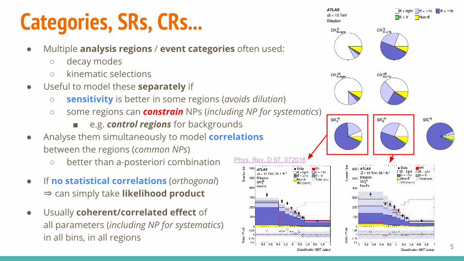
Categories, SRs, CRs...● Multiple analysis regions / event categories often used:
○ decay modes○ kinematic selections
● Useful to model these separately if○ sensitivity is better in some regions (avoids dilution)○ some regions can constrain NPs (including NP for systematics)
■ e.g. control regions for backgrounds● Analyse them simultaneously to model correlations
between the regions (common NPs)○ better than a-posteriori combination
● If no statistical correlations (orthogonal)⇒ can simply take likelihood product
● Usually coherent/correlated effect of all parameters (including NP for systematics)in all bins, in all regions
5
Phys. Rev. D 97, 072016
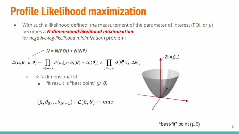
Profile Likelihood maximization● With such a likelihood defined, the measurement of the parameter of interest (POI, or µ)
becomes a N-dimensional likelihood maximisation (or negative-log-likelihood minimization) problem:
N = N(POI) + N(NP)
○ ⇒ N-dimensional fit■ fit result is "best point" (µ, θ)
6
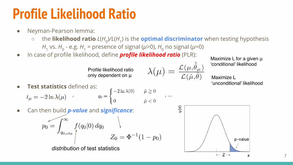
Profile Likelihood Ratio● Neyman-Pearson lemma:
○ the likelihood ratio L(H0)/L(H1) is the optimal discriminator when testing hypothesis H1 vs. H0 - e.g. H1 = presence of signal (µ>0), H0 no signal (µ=0)
● In case of profile likelihood, define profile likelihood ratio (PLR):
● Test statistics defined as: , , ...
● Can then build p-value and significance:
7
distribution of test statistics
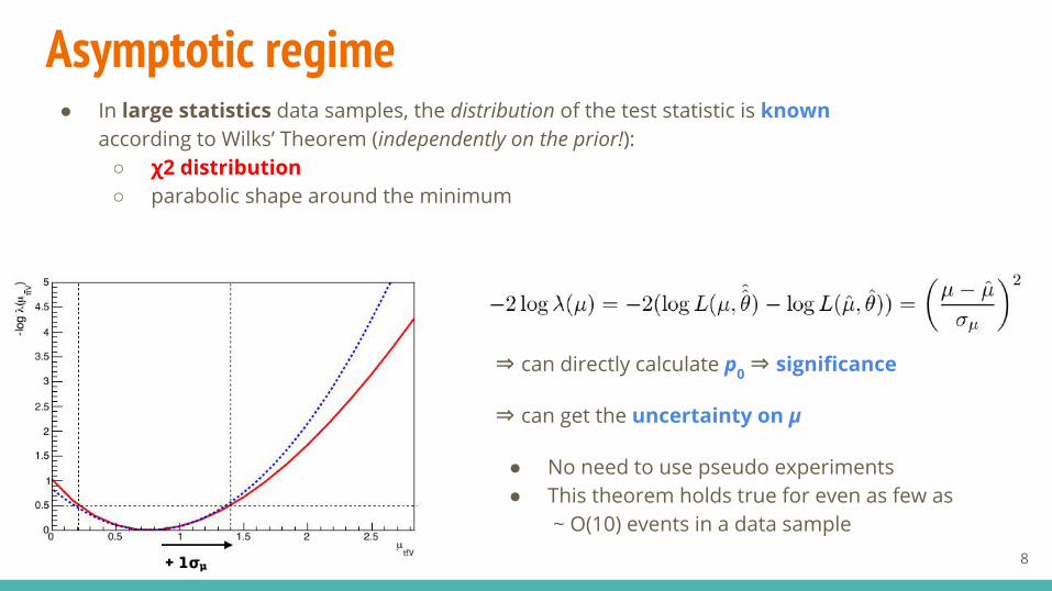
Asymptotic regime● In large statistics data samples, the distribution of the test statistic is known
according to Wilks’ Theorem (independently on the prior!):○ χ2 distribution○ parabolic shape around the minimum
⇒ can directly calculate p0 ⇒ significance
⇒ can get the uncertainty on µ
● No need to use pseudo experiments● This theorem holds true for even as few as
~ O(10) events in a data sample8

Profiling, pre-fit and post-fit● Profile likelihood fit can:
○ change background prediction, if best-fit θ values different from θ0 ○ reduce uncertainty on background, through:
■ constraint of NPs ("improved knowledge" of parameters that are affected by systematic uncertainties, i.e. data have enough statistical power to further constraint the NP)
■ correlations between NPs
9
FIT
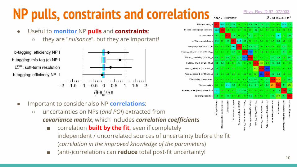
NP pulls, constraints and correlations● Useful to monitor NP pulls and constraints:
○ they are "nuisance", but they are important!
● Important to consider also NP correlations:○ uncertainties on NPs (and POI) extracted from
covariance matrix, which includes correlation coefficients■ correlation built by the fit, even if completely
independent / uncorrelated sources of uncertainty before the fit(correlation in the improved knowledge of the parameters)
■ (anti-)correlations can reduce total post-fit uncertainty!10
Phys. Rev. D 97, 072003
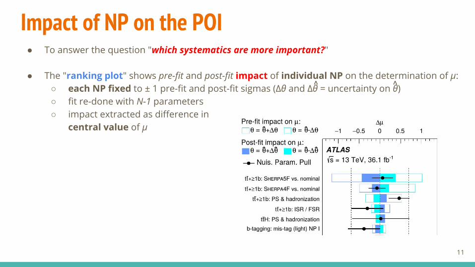
Impact of NP on the POI● To answer the question "which systematics are more important?"
● The "ranking plot" shows pre-fit and post-fit impact of individual NP on the determination of µ:○ each NP fixed to ± 1 pre-fit and post-fit sigmas (Δθ and Δθ = uncertainty on θ)○ fit re-done with N-1 parameters○ impact extracted as difference in
central value of µ
11
^ ^
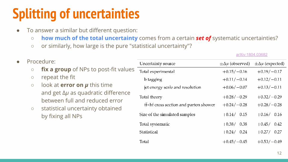
Splitting of uncertainties● To answer a similar but different question:
○ how much of the total uncertainty comes from a certain set of systematic uncertainties?○ or similarly, how large is the pure "statistical uncertainty"?
● Procedure:○ fix a group of NPs to post-fit values○ repeat the fit○ look at error on µ this time
and get Δµ as quadratic difference between full and reduced error
○ statistical uncertainty obtained by fixing all NPs
12
arXiv:1804.03682
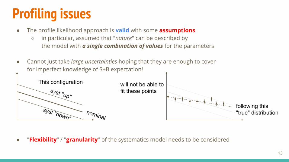
Profiling issues● The profile likelihood approach is valid with some assumptions
○ in particular, assumed that "nature" can be described by the model with a single combination of values for the parameters
● Cannot just take large uncertainties hoping that they are enough to cover for imperfect knowledge of S+B expectation!
● "Flexibility" / "granularity" of the systematics model needs to be considered
13
nominal
syst "up"
syst "down"
This configuration will not be able to fit these points
following this "true" distribution
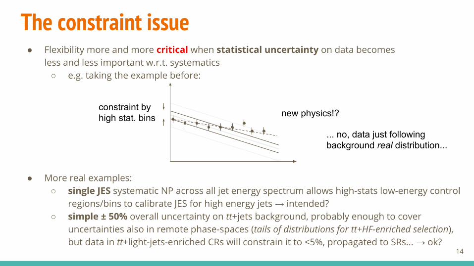
The constraint issue● Flexibility more and more critical when statistical uncertainty on data becomes
less and less important w.r.t. systematics○ e.g. taking the example before:
● More real examples:○ single JES systematic NP across all jet energy spectrum allows high-stats low-energy control
regions/bins to calibrate JES for high energy jets → intended?○ simple ± 50% overall uncertainty on tt+jets background, probably enough to cover
uncertainties also in remote phase-spaces (tails of distributions for tt+HF-enriched selection), but data in tt+light-jets-enriched CRs will constrain it to <5%, propagated to SRs... → ok?
14
constraint by high stat. bins new physics!?
... no, data just following background real distribution...

Theory modeling systematics● Experimental systematics nowadays often well suited for profile likelihood application:
○ come from calibrations ⇒ gaussian constraint appropriate○ broken-down into several independent/uncorrelated components (JES, b-tagging...)
● Different situation for theory systematics:○ difficulty 1: what is the distribution of the subsidiary measurement?○ difficulty 2: what are the parameters of the systematic?
■ can a combination of the included parameters describe any possible configuration?■ is any allowed value of the parameter physically meaningful?
● The obviously tricky case: "two point" systematics○ e.g. Herwig vs. Pythia as "parton shower and
hadronization model uncertainty",as a single NP
15
See: https://indico.cern.ch/event/287744/contributions/1641261/attachments/535763/738679/Verkerke_Statistics_3.pdf

Theory modeling systematics
16
One-bin case:- reasonable to think that "Sherpa"
can be between Herwig and Pythia
Shape case:- Sherpa can be different from linear
combination of Py and Her...
Which prior?
Pre-fit / non-constrained NP could be fine to cover for all possible models...
... but is this level of constraint ok?

Theory modeling systematics● A not-so-obviously tricky case:
○ scale uncertainties
17
Take NLO scale variations as uncertainty (missing NNLO MC)
+1
-1
⇒ flat uncertainty here, and NNLO is within uncertainty, but NNLO/NLO is not flat!
Suppose data looks like NNLO, we measure ytt, we constrain scale syst. in low ytt bins ⇒ new physics at high ytt?
Phys. Rev. Lett. 116, 082003

Systematics model validation● Especially given the impossibility to build a "perfect model", need to validate flexibility of
the adopted systematics model (better if before looking at the full data!)
● Response of the model to injection tests:○ build toy data (or Asimov data) with non-nominal properties
■ can vary parameters of the model (i.e. by shifting NPs when creating the Asimov data-set)
■ can use a MC generator not included in the systematics model to build the toy data
■ check compatibility of best-fit POI with injected value
● Post-fit plots:○ evaluate data/prediction agreement across distributions with fit result projection
(shifted prediction + reduced systematics band)○ can spot issues e.g. if found disagreement in a region where don't expect signal○ especially useful for validation regions / validation distributions
i.e. regions / distributions not directly used in the fit
● Mention for sure the test with modified Asimov dataset (from alternative MC sample for one or more backgrounds, not used in the definition of systematics model)
○ very useful to probe the flexibility of the fit model
18
Fit Fit FitAsimov
S+BAsimov'
S+B(θ=θ') Asimov''
S+B'
^µ = 1
^µ'
^µ''
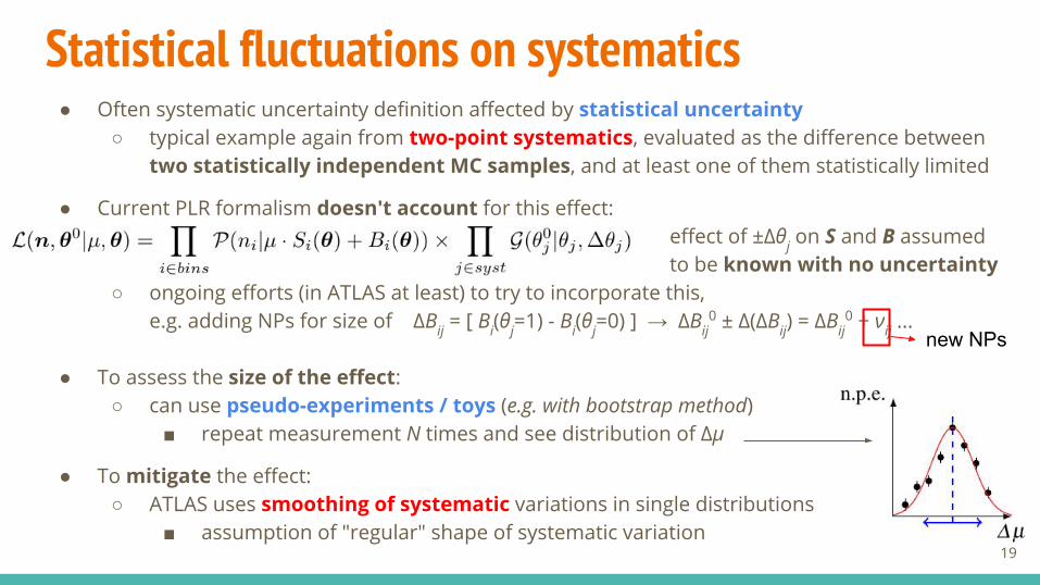
Statistical fluctuations on systematics● Often systematic uncertainty definition affected by statistical uncertainty
○ typical example again from two-point systematics, evaluated as the difference between two statistically independent MC samples, and at least one of them statistically limited
● Current PLR formalism doesn't account for this effect:effect of ±Δθj on S and B assumed to be known with no uncertainty
○ ongoing efforts (in ATLAS at least) to try to incorporate this, e.g. adding NPs for size of ΔBij = [ Bi(θj=1) - Bi(θj=0) ] → ΔBij
0 ± Δ(ΔBij) = ΔBij0 + νij ...
● To assess the size of the effect:○ can use pseudo-experiments / toys (e.g. with bootstrap method)
■ repeat measurement N times and see distribution of Δµ
● To mitigate the effect:○ ATLAS uses smoothing of systematic variations in single distributions
■ assumption of "regular" shape of systematic variation19
new NPs
Including data-driven estimates into the fit model● Often data-driven estimates provided as inputs for the PLR model
○ however, ideally better to include the estimate in the fit model■ easier handling of correlations■ natural way of considering signal contamination in control region
○ not always possible/easy (example: Matrix Method for fakes and non-prompt lepton background determination)
● With more and more data, natural to consider more and more data-driven or partially data-driven background estimation techniques, also for backgrounds currently estimated through MC and with NPs constrained by the data
○ by building more data-driven predictions, possibly included in the PLR model, could reduce issues related to over-constraints of NPs and enhance model flexibility
20
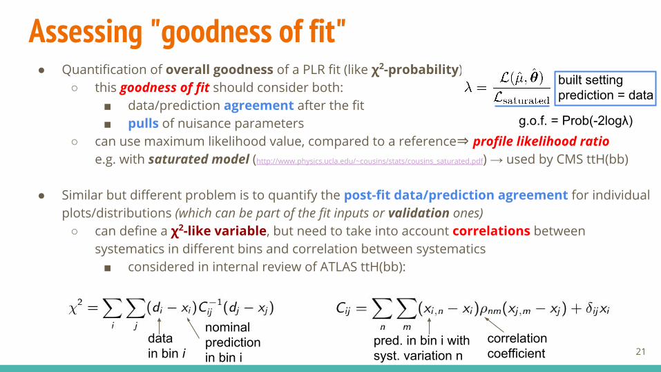
Assessing "goodness of fit"● Quantification of overall goodness of a PLR fit (like χ2-probability)
○ this goodness of fit should consider both:■ data/prediction agreement after the fit■ pulls of nuisance parameters
○ can use maximum likelihood value, compared to a reference⇒ profile likelihood ratioe.g. with saturated model (http://www.physics.ucla.edu/~cousins/stats/cousins_saturated.pdf) → used by CMS ttH(bb)
● Similar but different problem is to quantify the post-fit data/prediction agreement for individual plots/distributions (which can be part of the fit inputs or validation ones)
○ can define a χ2-like variable, but need to take into account correlations between systematics in different bins and correlation between systematics
■ considered in internal review of ATLAS ttH(bb):
21data in bin i
nominal prediction in bin i
correlation coefficient
pred. in bin i with syst. variation n
g.o.f. = Prob(-2logλ)
built setting prediction = data

Combination of measurements● With the PLR approach, combination of different
measurements is natural:○ "just" add some more bins to the product
● However, important to consider compatibility of models:○ orthogonality of channels:
■ bin contents in PLR are supposed to be statistically independent
○ same definition of (set of) POI:■ sometimes obvious, but not always
(is µ applied to all the ttH, or just one decay channel? What about tH? ...)○ compatible set of systematics:
■ this is the most tricky part, especially for ATLAS+CMS combinations!■ mainly dealing with the question "which NPs are correlated between channels?"■ often cannot reach perfect solution, need to test different correlation assumptions
(notice that in PLR formalism systematics are either fully correlated or fully uncorrelated...)22

Summary and conclusions● Profile likelihood ratio (PLR) approach presented, in the context of ttH analyses
(mainly in the "binned case", i.e. ttH(bb) and multi-lepton channels)○ tod, mefeatures and possible pitfalls discussed
● Room for fruitful discussion on the most critical points in these days○ important to consider how the current approach will work and eventually evolve with:
■ more and more data■ more and more precision measurements■ more and more accurate/refined/rich theory predictions■ new experimental analysis techniques...
23

Backup
24

NP interpolation / extrapolation● The "NP interpolation / extrapolation" controls how a variation of a NP θj reflects in a
variation of the predicted yields (S(θj) and B(θj), in the various bins)● Different schemes / codes are implemented in RooStats/RooFit, e.g.:
○ piecewise linear → default for shape component of systematics○ polynomial interpolation / exponential extrapolation → default for norm. component
θ θ
B(θ) B(θ)
25
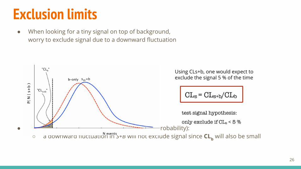
Exclusion limits● When looking for a tiny signal on top of background,
worry to exclude signal due to a downward fluctuation
● So we use CLs to test a signal hypothesis (not a probability):○ a downward fluctuation in S+B will not exclude signal since CLb will also be small
Using CLs+b, one would expect toexclude the signal 5 % of the time
26
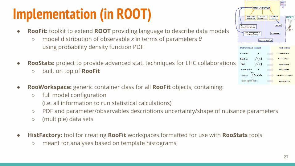
Implementation (in ROOT)● RooFit: toolkit to extend ROOT providing language to describe data models
○ model distribution of observable x in terms of parameters θ using probability density function PDF
● RooStats: project to provide advanced stat. techniques for LHC collaborations○ built on top of RooFit
● RooWorkspace: generic container class for all RooFit objects, containing:○ full model configuration
(i.e. all information to run statistical calculations)○ PDF and parameter/observables descriptions uncertainty/shape of nuisance parameters○ (multiple) data sets
● HistFactory: tool for creating RooFit workspaces formatted for use with RooStats tools○ meant for analyses based on template histograms
27