Athens University of Economics and Business Dynamic ... · The Distinguishing Feature of the Keynesian Approach In the Keynesian models, the immediate adjustment of prices and wages

Athens University of Economics and Business

13. Keynesian Models and the Phillips Curve

Dynamic Macroeconomics

Prof. George Alogoskoufis

alogoskoufisg.com

George Alogoskoufis, Dynamic Macroeconomics, 2019

http://alogoskoufisg.com


The Keynesian ApproachFollowing the Great Depression of the 1930s, the analysis of aggregate fluctuations developed into macroeconomics, on the basis of so-called keynesian models.

These models, were derived from the General Theory of Keynes (1936), who argued against the then prevailing “classical” equilibrium theory of employment and aggregate fluctuations.

Keynes proceeded to argue that a general theory, as opposed to the classical theory, ought to be able to explain involuntary unemployment, which he proceeded to duly define as a situation in which the real wage is higher than the marginal disutility of labor.

The Keynesian approach was developed through a sequence of models in the General Theory.

2


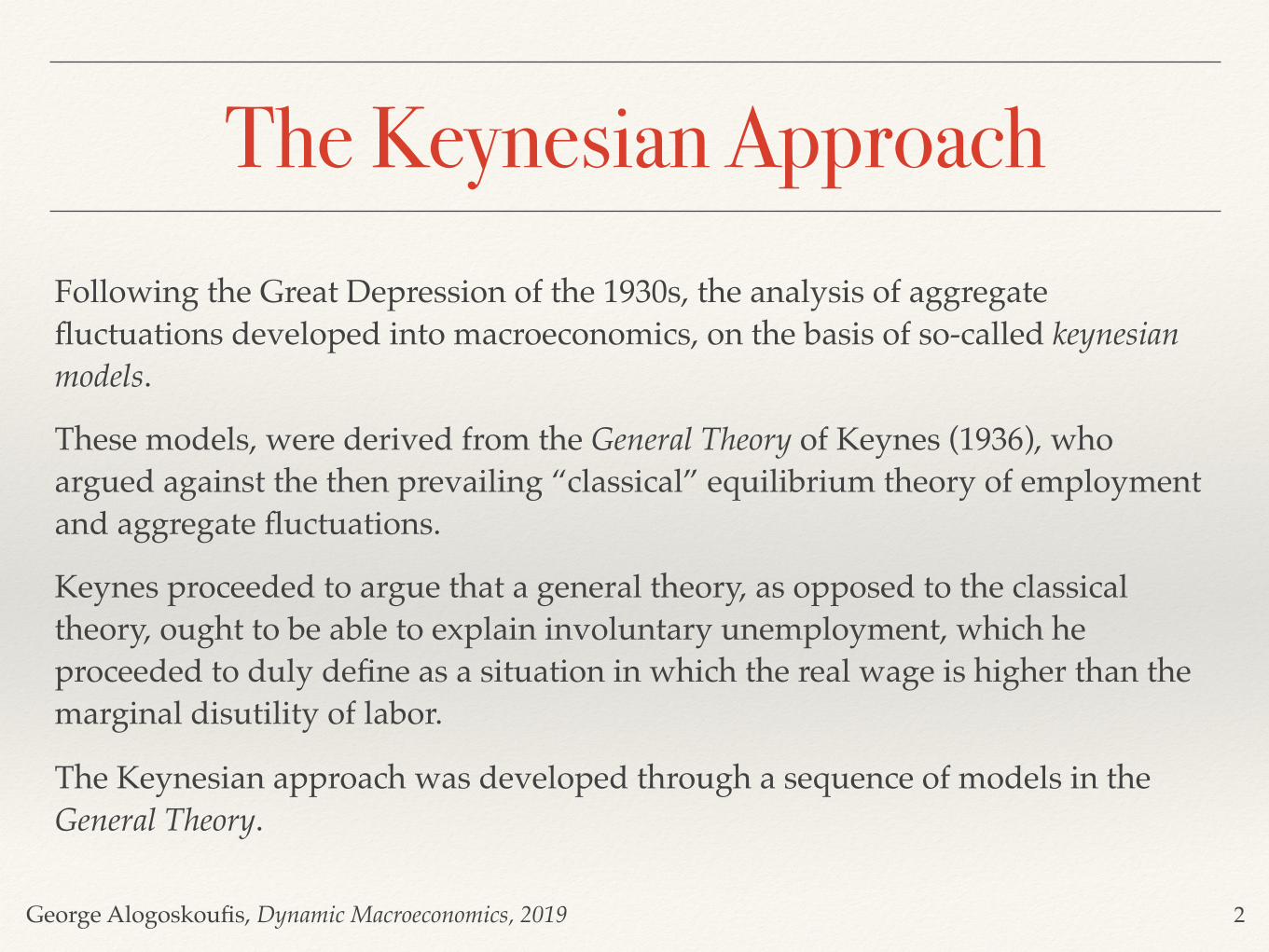
Keynes, John Maynard (1883-1946)The ideas of Keynes, an English economist, fundamentally changed the theory and practice of macroeconomics and the economic policies of governments.

In his 1936 book, The General Theory of Employment, Interest and Money, Keynes spearheaded a revolution in economic thinking, challenging the ideas of neoclassical economics which held that free markets would, in the short to medium term, automatically provide full employment, as long as workers were flexible in their wage demands. He instead argued that in the short to medium run aggregate demand determined the overall level of economic activity and that inadequate aggregate demand could lead to prolonged periods of high unemployment.

He built on and greatly refined earlier work on the causes of business cycles, and is widely considered to be one of the most influential economists of the 20th century and the founder of modern macroeconomics.

3


The Three Models of the ‘General Theory’

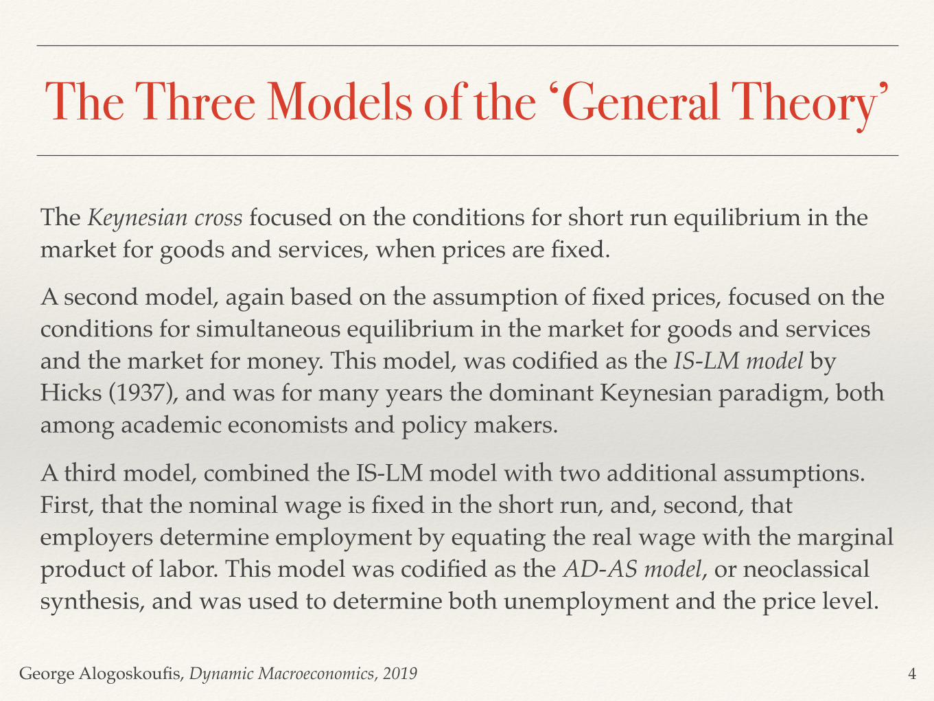
The Keynesian cross focused on the conditions for short run equilibrium in the market for goods and services, when prices are fixed.

A second model, again based on the assumption of fixed prices, focused on the conditions for simultaneous equilibrium in the market for goods and services and the market for money. This model, was codified as the IS-LM model by Hicks (1937), and was for many years the dominant Keynesian paradigm, both among academic economists and policy makers.

A third model, combined the IS-LM model with two additional assumptions. First, that the nominal wage is fixed in the short run, and, second, that employers determine employment by equating the real wage with the marginal product of labor. This model was codified as the AD-AS model, or neoclassical synthesis, and was used to determine both unemployment and the price level.

4


The Distinguishing Feature of the Keynesian Approach

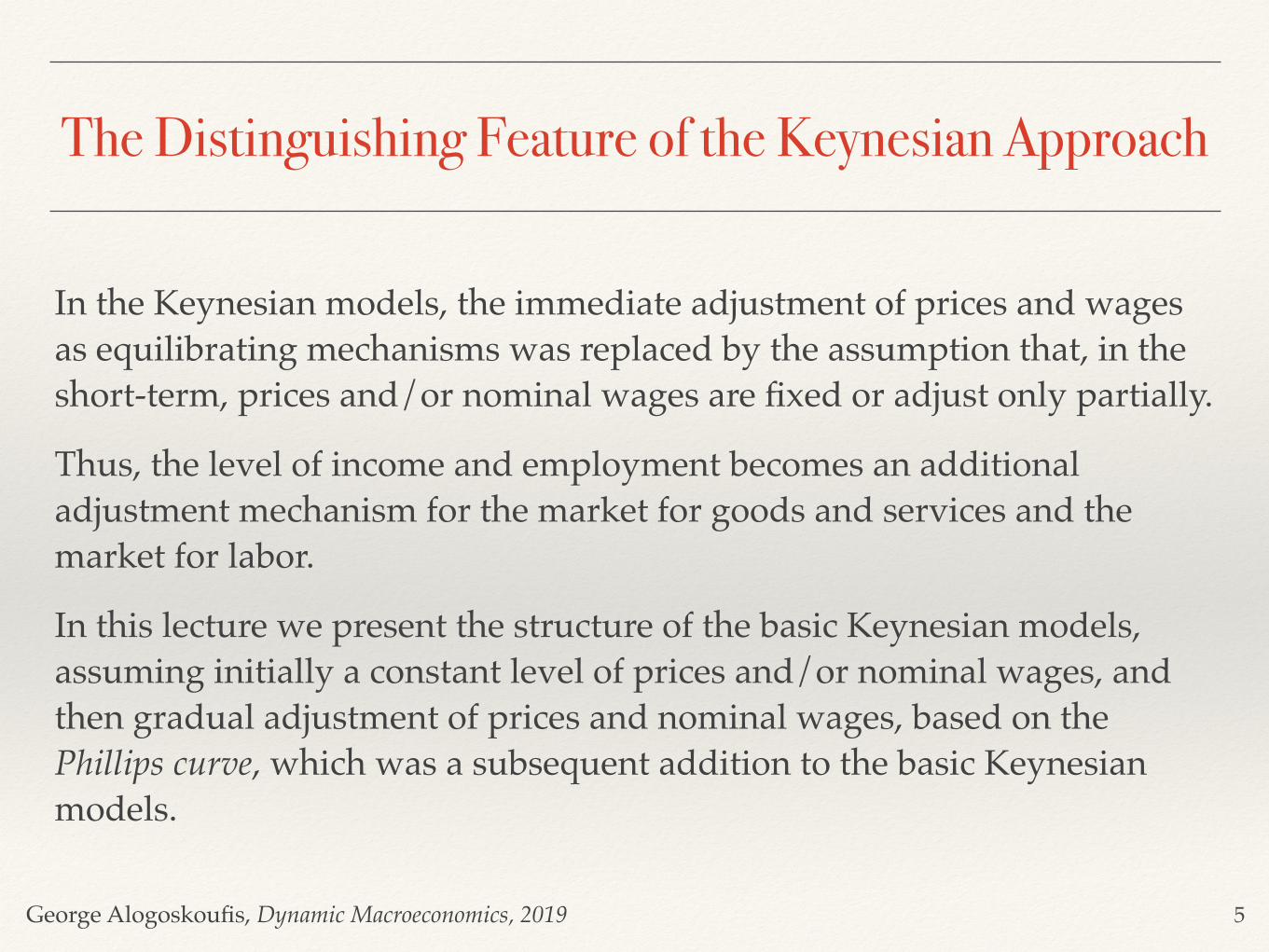
In the Keynesian models, the immediate adjustment of prices and wages as equilibrating mechanisms was replaced by the assumption that, in the short-term, prices and/or nominal wages are fixed or adjust only partially.

Thus, the level of income and employment becomes an additional adjustment mechanism for the market for goods and services and the market for labor.

In this lecture we present the structure of the basic Keynesian models, assuming initially a constant level of prices and/or nominal wages, and then gradual adjustment of prices and nominal wages, based on the Phillips curve, which was a subsequent addition to the basic Keynesian models.

5


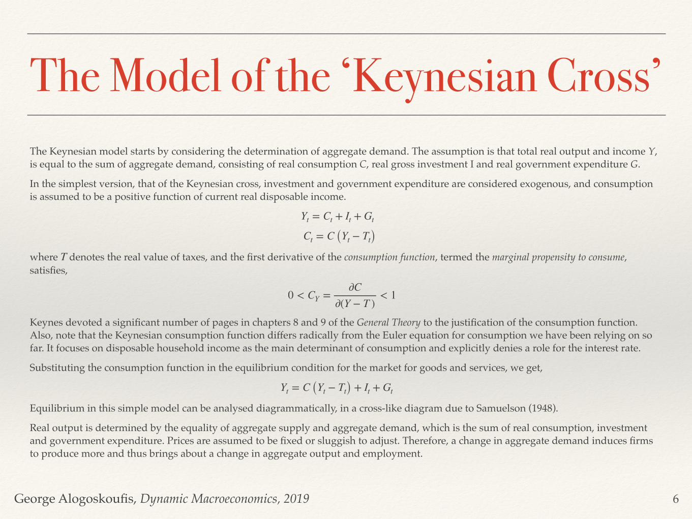
The Model of the ‘Keynesian Cross’The Keynesian model starts by considering the determination of aggregate demand. The assumption is that total real output and income Y, is equal to the sum of aggregate demand, consisting of real consumption C, real gross investment Ι and real government expenditure G.

In the simplest version, that of the Keynesian cross, investment and government expenditure are considered exogenous, and consumption is assumed to be a positive function of current real disposable income.

where denotes the real value of taxes, and the first derivative of the consumption function, termed the marginal propensity to consume, satisfies,

Keynes devoted a significant number of pages in chapters 8 and 9 of the General Theory to the justification of the consumption function. Also, note that the Keynesian consumption function differs radically from the Euler equation for consumption we have been relying on so far. It focuses on disposable household income as the main determinant of consumption and explicitly denies a role for the interest rate.

Substituting the consumption function in the equilibrium condition for the market for goods and services, we get,

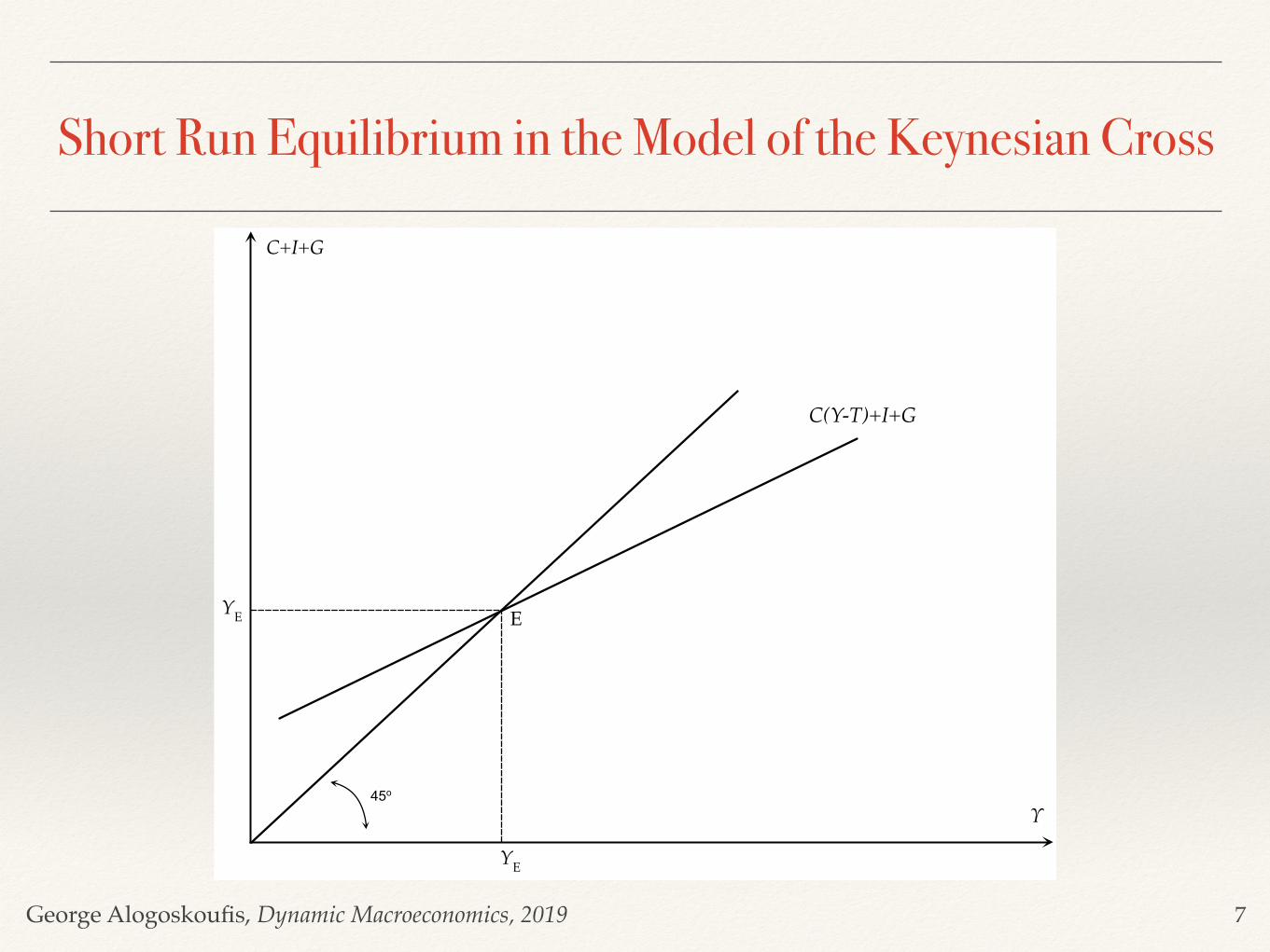
Equilibrium in this simple model can be analysed diagrammatically, in a cross-like diagram due to Samuelson (1948).

Real output is determined by the equality of aggregate supply and aggregate demand, which is the sum of real consumption, investment and government expenditure. Prices are assumed to be fixed or sluggish to adjust. Therefore, a change in aggregate demand induces firms to produce more and thus brings about a change in aggregate output and employment.

Yt = Ct + It + Gt

Ct = C (Yt − Tt)T

0 < CY =∂C

∂(Y − T )< 1

Yt = C (Yt − Tt) + It + Gt

6


Short Run Equilibrium in the Model of the Keynesian Cross

7

C+I+G

Υ

YΕ

YΕ E

45o

C(Y-T)+I+G


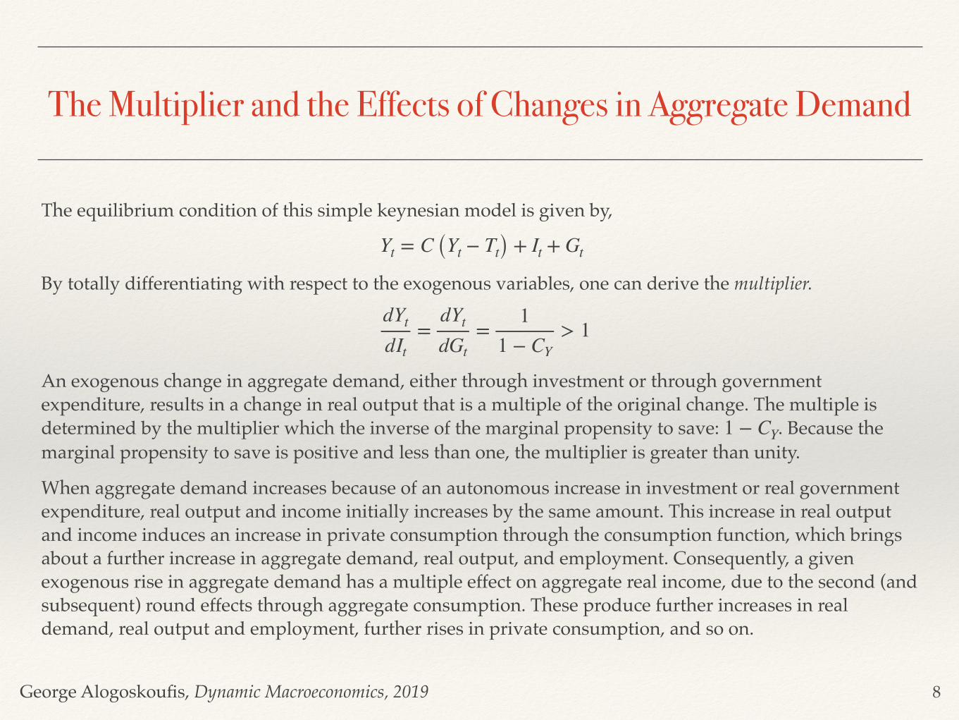
The Multiplier and the Effects of Changes in Aggregate Demand

The equilibrium condition of this simple keynesian model is given by,

By totally differentiating with respect to the exogenous variables, one can derive the multiplier.

An exogenous change in aggregate demand, either through investment or through government expenditure, results in a change in real output that is a multiple of the original change. The multiple is determined by the multiplier which the inverse of the marginal propensity to save: . Because the marginal propensity to save is positive and less than one, the multiplier is greater than unity.

When aggregate demand increases because of an autonomous increase in investment or real government expenditure, real output and income initially increases by the same amount. This increase in real output and income induces an increase in private consumption through the consumption function, which brings about a further increase in aggregate demand, real output, and employment. Consequently, a given exogenous rise in aggregate demand has a multiple effect on aggregate real income, due to the second (and subsequent) round effects through aggregate consumption. These produce further increases in real demand, real output and employment, further rises in private consumption, and so on.

Yt = C (Yt − Tt) + It + Gt

dYt

dIt=

dYt

dGt=

11 − CY

> 1

1 − CY

8


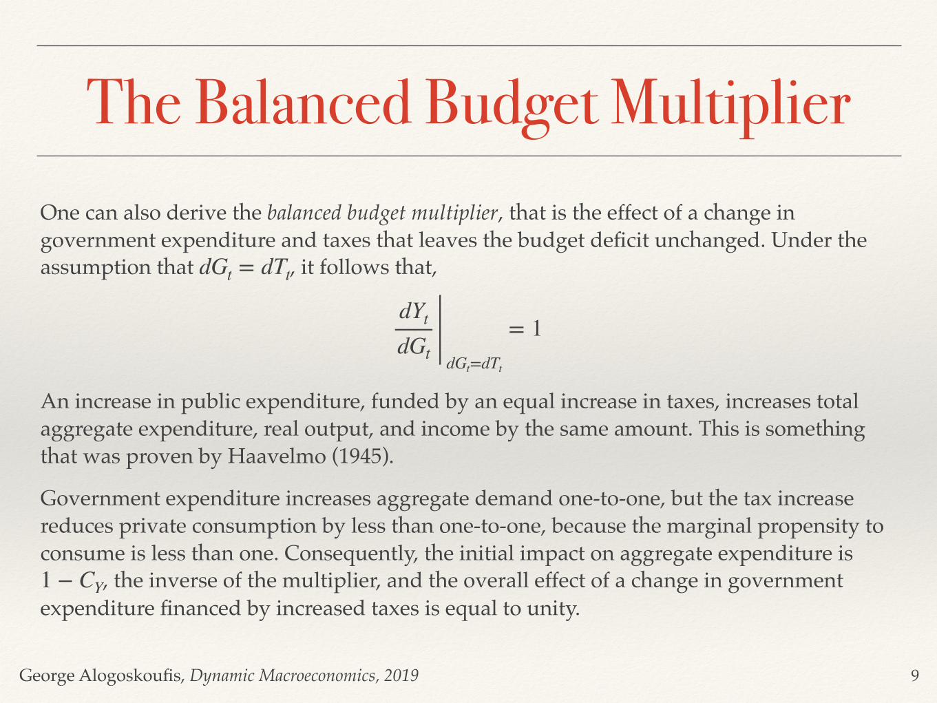
The Balanced Budget MultiplierOne can also derive the balanced budget multiplier, that is the effect of a change in government expenditure and taxes that leaves the budget deficit unchanged. Under the assumption that , it follows that,

An increase in public expenditure, funded by an equal increase in taxes, increases total aggregate expenditure, real output, and income by the same amount. This is something that was proven by Haavelmo (1945).

Government expenditure increases aggregate demand one-to-one, but the tax increase reduces private consumption by less than one-to-one, because the marginal propensity to consume is less than one. Consequently, the initial impact on aggregate expenditure is

, the inverse of the multiplier, and the overall effect of a change in government expenditure financed by increased taxes is equal to unity.

dGt = dTt

dYt

dGt dGt=dTt

= 1

1 − CY

9


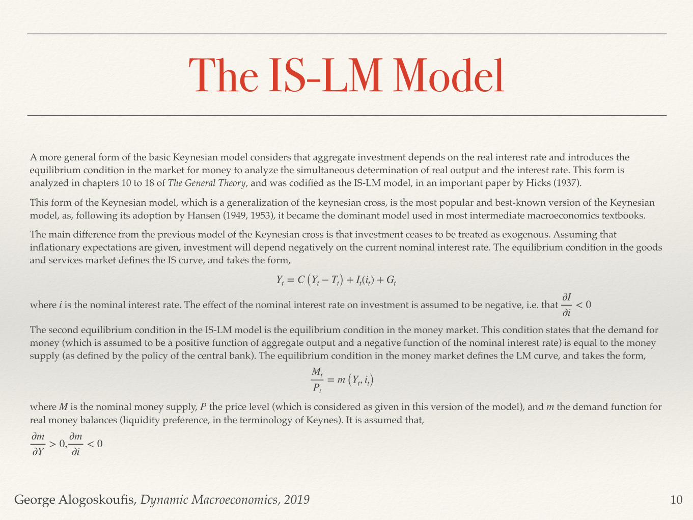
The IS-LM ModelA more general form of the basic Keynesian model considers that aggregate investment depends on the real interest rate and introduces the equilibrium condition in the market for money to analyze the simultaneous determination of real output and the interest rate. This form is analyzed in chapters 10 to 18 of The General Theory, and was codified as the IS-LM model, in an important paper by Hicks (1937).

This form of the Keynesian model, which is a generalization of the keynesian cross, is the most popular and best-known version of the Keynesian model, as, following its adoption by Hansen (1949, 1953), it became the dominant model used in most intermediate macroeconomics textbooks.

The main difference from the previous model of the Keynesian cross is that investment ceases to be treated as exogenous. Assuming that inflationary expectations are given, investment will depend negatively on the current nominal interest rate. The equilibrium condition in the goods and services market defines the IS curve, and takes the form,

where is the nominal interest rate. The effect of the nominal interest rate on investment is assumed to be negative, i.e. that

The second equilibrium condition in the IS-LM model is the equilibrium condition in the money market. This condition states that the demand for money (which is assumed to be a positive function of aggregate output and a negative function of the nominal interest rate) is equal to the money supply (as defined by the policy of the central bank). The equilibrium condition in the money market defines the LM curve, and takes the form,

where is the nominal money supply, the price level (which is considered as given in this version of the model), and the demand function for real money balances (liquidity preference, in the terminology of Keynes). It is assumed that,

Yt = C (Yt − Tt) + It(it) + Gt

i∂I∂i

< 0

Mt

Pt= m (Yt, it)

M P m

∂m∂Y

> 0,∂m∂i

< 0

10


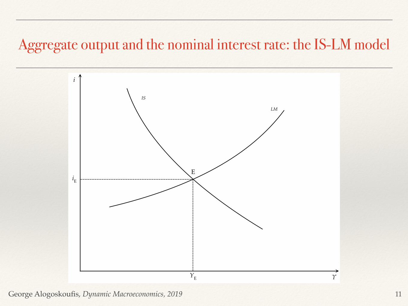
Aggregate output and the nominal interest rate: the IS-LM model

11

i

ΥYΕ

iΕE

IS

LM


The IS-LM Model and the Effects of Monetary and Fiscal Policy

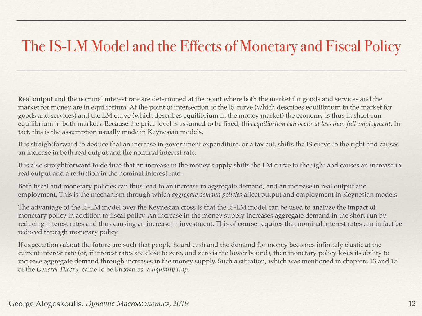
Real output and the nominal interest rate are determined at the point where both the market for goods and services and the market for money are in equilibrium. At the point of intersection of the IS curve (which describes equilibrium in the market for goods and services) and the LM curve (which describes equilibrium in the money market) the economy is thus in short-run equilibrium in both markets. Because the price level is assumed to be fixed, this equilibrium can occur at less than full employment. In fact, this is the assumption usually made in Keynesian models.

It is straightforward to deduce that an increase in government expenditure, or a tax cut, shifts the IS curve to the right and causes an increase in both real output and the nominal interest rate.

It is also straightforward to deduce that an increase in the money supply shifts the LM curve to the right and causes an increase in real output and a reduction in the nominal interest rate.

Both fiscal and monetary policies can thus lead to an increase in aggregate demand, and an increase in real output and employment. This is the mechanism through which aggregate demand policies affect output and employment in Keynesian models.

The advantage of the IS-LM model over the Keynesian cross is that the IS-LM model can be used to analyze the impact of monetary policy in addition to fiscal policy. An increase in the money supply increases aggregate demand in the short run by reducing interest rates and thus causing an increase in investment. This of course requires that nominal interest rates can in fact be reduced through monetary policy.

If expectations about the future are such that people hoard cash and the demand for money becomes infinitely elastic at the current interest rate (or, if interest rates are close to zero, and zero is the lower bound), then monetary policy loses its ability to increase aggregate demand through increases in the money supply. Such a situation, which was mentioned in chapters 13 and 15 of the General Theory, came to be known as a liquidity trap.

12


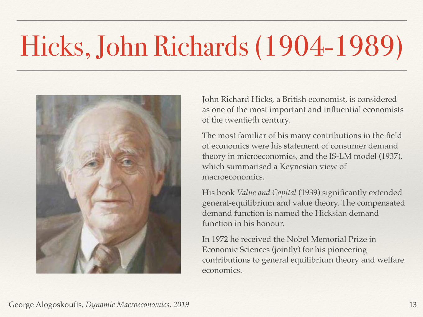
Hicks, John Richards (1904-1989)John Richard Hicks, a British economist, is considered as one of the most important and influential economists of the twentieth century.

The most familiar of his many contributions in the field of economics were his statement of consumer demand theory in microeconomics, and the IS-LM model (1937), which summarised a Keynesian view of macroeconomics.

His book Value and Capital (1939) significantly extended general-equilibrium and value theory. The compensated demand function is named the Hicksian demand function in his honour.

In 1972 he received the Nobel Memorial Prize in Economic Sciences (jointly) for his pioneering contributions to general equilibrium theory and welfare economics.

13


The AD-AS ModelThe last and most sophisticated form of the basic Keynesian model is analyzed in chapters 19-21 of the General Theory. In this form of the model, the price level ceases to be exogenous and is allowed to change in order to equilibrate aggregate demand for goods and services with a less-than-perfectly elastic aggregate supply curve. However, nominal wages are still considered to be fixed in the short run. This version of the model was formally combined with the IS-LM framework by Modigliani (1944) and has been known as the aggregate demand-aggregate supply (AD-AS) model.

The aggregate demand function (AD) is derived from the simultaneous satisfaction of the equilibrium condition in the market for goods and services (IS) and the equilibrium condition in the money market (LM). Substituting out for the nominal interest rate between the two, we get an aggregate demand function of the form,

, where, .

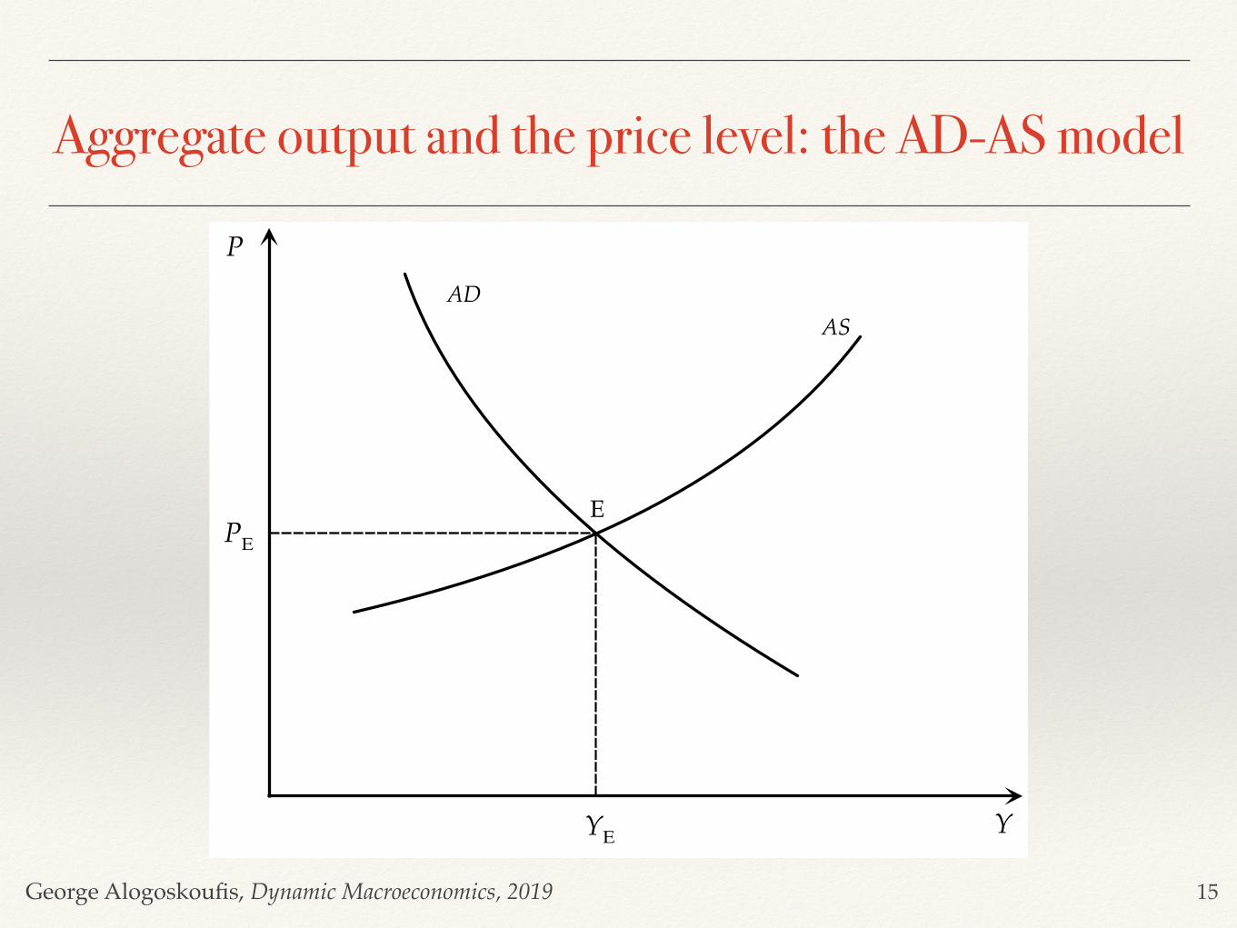
This describes the aggregate demand curve as a negative function of the price level . A higher price level, given the money supply, means lower real money balances, higher nominal interest rates, and lower investment demand. Thus, given the money supply, an increase in the price level reduces aggregate demand, and a fall in the price level increases aggregate demand.

To derive the aggregate supply function (AS), we examine the behavior of the representative firm. Assume that the representative firm is competitive and maximizes profits, selecting the level of employment and output, taking nominal wages and prices as given. From the first-order conditions for maximum profits, the firm equates the marginal product of labor to the real wage. If the production function is subject to diminishing returns to labor, labor demand is a negative function of the real wage. Hence, output is a negative function of the real wage. If the nominal wage is fixed in the short-run, the supply of output is a positive function of the price level. Hence,

, where,

The higher the level of prices is, the lower the real wage will be, with the result that the aggregate supply curve AS is upward sloping in .

Yt = D ( Mt

Pt, Gt, Tt) ∂D

∂Pt< 0

P

Yt = S ( WPt ) ∂S

∂Pt> 0

P

14


Aggregate output and the price level: the AD-AS model

15

P

YYΕ

PΕE

ADAS


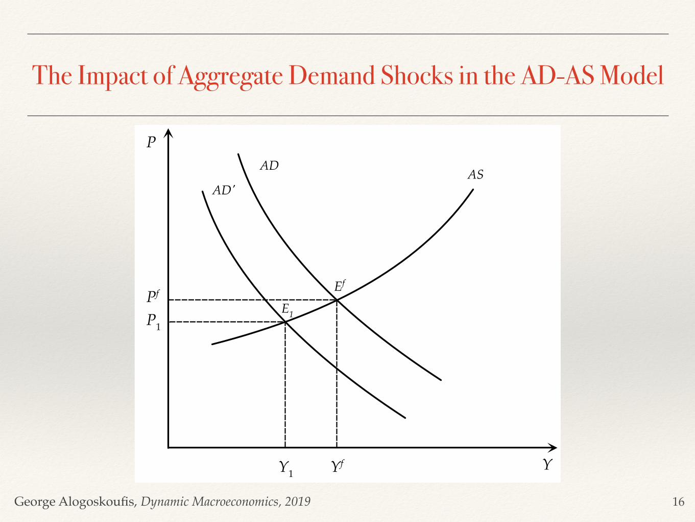
The Impact of Aggregate Demand Shocks in the AD-AS Model

16

P

YYf

Pf Ef

AD AS

P1E1

Y1

AD'


Aggregate Demand Shocks and Aggregate Demand Policies

In contrast to the ‘classical’ model of full adjustment of wages and prices, in the keynesian model with nominal wage rigidity, even monetary disturbances can shift aggregate demand and cause fluctuations in real output, employment, and other real variables (such as real wages and interest rates).

How can the impact of shocks to aggregate demand and supply be addressed? According to the keynesian approach, an appropriate solution can come from macroeconomic policy.

An increase of government expenditure, a reduction in taxes, or an increase in the money supply can move the aggregate demand curve to the right and counteract the consequences of a negative demand or supply shock on real output and unemployment.

In the case of demand shocks, the price level returns to its original equilibrium. In the case of a negative supply shock there are further upward effects on the price level, so a trade-off occurs between unemployment and price stability.

Thus, supply shocks cannot be effectively neutralized through aggregate demand policies, as trying to counteract them through aggregate demand policies has implications for the price level. In the case of a positive demand or supply shock, the opposite would apply.

We shall return to the question of role of aggregate demand policies in Keynesian models after we examine the Samuelson (1939) multiplier-accelerator model, which is a dynamic version of the model of the Keynesian cross.

17


The Samuelson Multiplier-Accelerator Model

All versions of the Keynesian model we have considered so far are essentially static short-run equilibrium models. In an important paper, Samuelson (1939) combined the model of the keynesian cross with an investment function based on the principle of acceleration to derive a dynamic model of endogenous business cycles. This dynamic Keynesian model is known as the multiplier-accelerator model.

Samuelson considered the following dynamic version of the model of the Keynesian cross:

where are constant parameters. is the accelerator, which determines how a change in consumption affects current investment, and is autonomous investment. is the marginal propensity to consume, and is autonomous consumption. Finally is government expenditure, assumed exogenous and constant.

The investment function is based on the so-called acceleration principle, which implies that when there is a positive change in consumption, firms will invest more to produce the higher quantity of consumer goods demanded. When there is a negative change in consumption, firms will reduce investment, as they need less capital to meet the lower demand for consumer goods. The accelerator measures the sensitivity of investment to changes in aggregate consumption. The principle of acceleration, as a basis for a theory of investment, has a long history in the analysis of business cycles, but by current standards it is entirely ad hoc, as its microeconomic foundations are weak.The consumption function, according to which consumption is a function of lagged and not current income is a linear dynamic version of the keynesian consumption function. Government expenditure is assumed exogenous and constant at .

Yt = Ct + It + Gt

It = a(Ct − Ct−1) + b

Ct = cYt−1 + d

Gt = e

a, b, c, d, e ab c d e

a

e

18


Samuelson, Paul Anthony (1915-2009)

Paul Anthony Samuelson (May 15, 1915 – December 13, 2009) was an American economist who is widely considered to be the most influential economist of the second part of the 20th century.

The Swedish Royal Academy stated, when awarding the Nobel prize to him in 1970, that he "has done more than any other contemporary economist to raise the level of scientific analysis in economic theory”.

Samuelson considered mathematics to be the "natural language" for economists and contributed significantly to the mathematical foundations of economics with his 1946 book Foundations of Economic Analysis.

He was author of the best-selling economics textbook of all time, Economics, first published in 1948. It was the second American textbook that attempted to explain the principles of Keynesian economics.

19


Output Fluctuations in the Multiplier-Accelerator Model

Using the consumption function, the investment function and the assumption about government expenditure to eliminate , and from the product market equilibrium condition, we get,

The dynamic path of output in the Samuelson model is thus determined by a second-order difference equation.

The particular solution of this equation, which defines equilibrium output, is given by,

Equilibrium output depends only on autonomous expenditure and the multiplier , as suggested by the model of the Keynesian cross. However, the dynamic path of output is determined by a second-order difference equation which also depends on the accelerator.

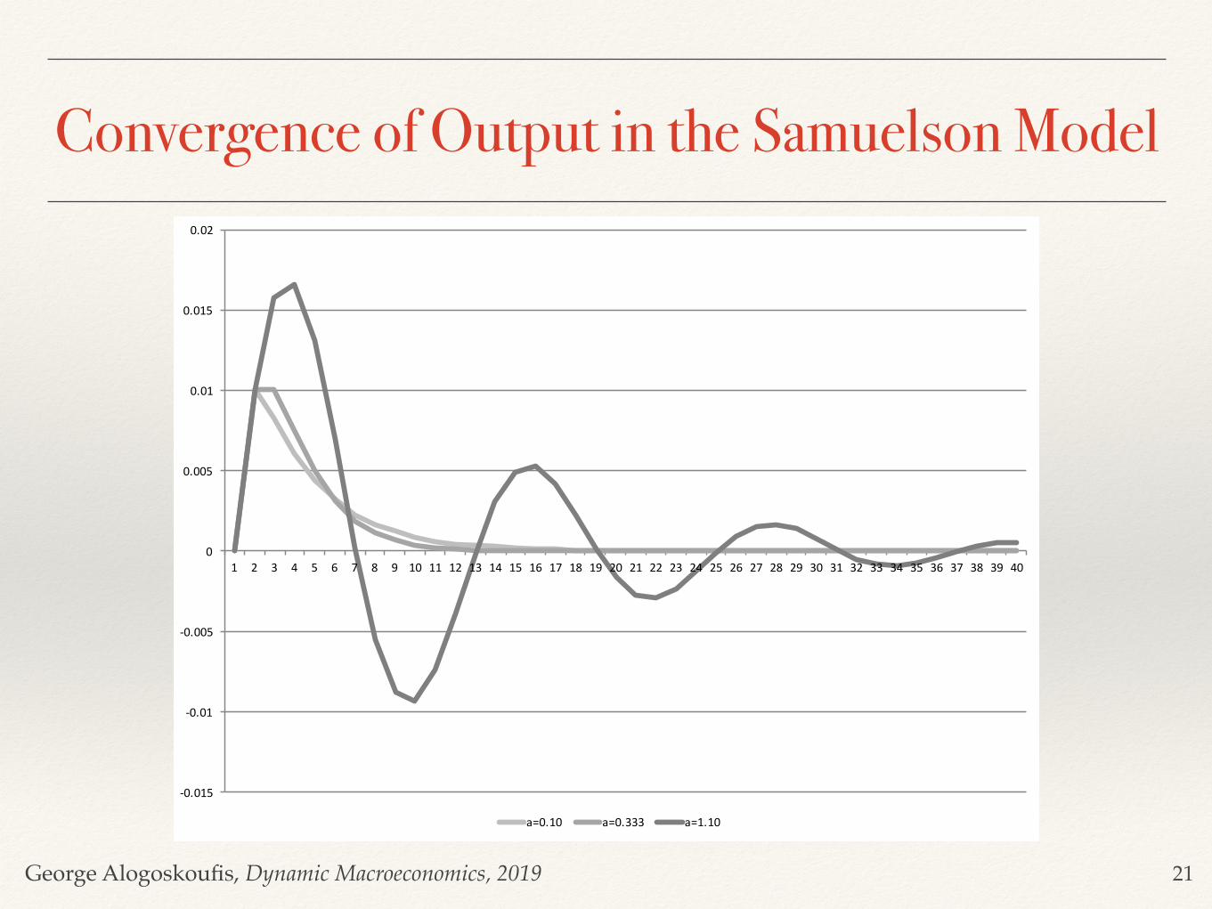
For the difference equation to be stable, must be less than one, or the accelerator must satisfy . If this condition is not satisfied, output will not converge to equilibrium but will instead diverge.

For the roots to be real, we must have that, . Thus, for the roots to be real and for income to converge monotonically to its equilibrium value, the condition is,

In the case where the inequality on the left-hand side is not satisfied, then we shall have two complex roots , and real output will display damped oscillations (i.e., endogenous fluctuations) during the convergence to its equilibrium value. This will occur as long as . If the accelerator does not satisfy this condition, then the model displays divergent oscillations.

The figure on the next slide shows the dynamic convergence of real output for different values of the accelerator, assuming .

C I G

Yt = c(1 + a)Yt−1 − acYt−2 + b + d + e

Y* =b + d + e

1 − c1/(1 − c)

ac a < 1/c

c ≥ 4a /(1 + a)2

4a(1 + a)2 ≤ c <

1a

λ1 λ2a < 1/c

c = 0.75

20


Convergence of Output in the Samuelson Model

21

-0.015

-0.01

-0.005

0

0.005

0.01

0.015

0.02

1 2 3 4 5 6 7 8 9 10 11 12 13 14 15 16 17 18 19 20 21 22 23 24 25 26 27 28 29 30 31 32 33 34 35 36 37 38 39 40

a=0.10 a=0.333 a=1.10


The Phillips Curve and the Tradeoff between Inflation and Unemployment

Since the late 1950s, a central point of reference for Keynesian models has been the Phillips curve, a negative relationship between unemployment and inflation, identified and estimated econometrically by Phillips (1958). The Phillips curve was combined with the IS-LM model of aggregate demand to simultaneously determine both inflation and unemployment. Thus, the Phillips curve essentially replaced the aggregate supply curve of the AD-AS model, which was based on fixed nominal wages, and helped determine both unemployment and inflation.

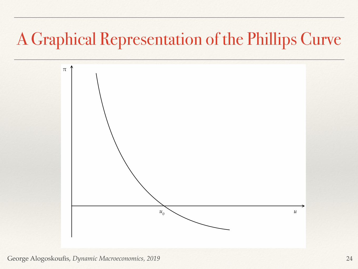
The curve that Phillips estimated econometrically, for the United Kingdom, took the form,

where and . In the Phillips curve denotes inflation, the unemployment rate, and is the zero inflation unemployment rate. The function relating inflation and unemployment estimated by Phillips was non-linear.

In the context of the basic Keynesian model, combining the IS-LM model of the determination of aggregate demand with the Phillips curve, one could deduce that an increase in aggregate demand would lead to higher real output and employment, lower unemployment, and a rise in inflation along the Phillips curve. Conversely, a decline in aggregate demand would lead to a lower level of real output and employment, higher unemployment, and a reduction of inflation along the Phillips curve.

Inspired by Phillips (1958), Samuelson and Solow (1960), estimated a Phillips curve between price inflation and unemployment in the United States. These authors argued that the short-term problem of macroeconomic policy could be seen as the determination of the level of aggregate demand, in order to select the socially desirable combination of inflation and unemployment on the Phillips curve. In times of recession, an increase in aggregate demand will lead to a reduction in unemployment, but at the cost of higher inflation. In times of economic boom and high inflation, inflation could be reduced through a reduction in aggregate demand, but this would result in higher unemployment.

π = φ(u)

φ(u0) = 0 φ′�(u) < 0 π u u0φ

22


Phillips, Alban William (1914-1975)

Phiilips was a New Zealand economist who spent most of his academic career as a professor of economics at the London School of Economics (LSE).

His best-known contribution to economics is the Phillips curve, which he first described in 1958.

He also designed and built the MONIAC hydraulic economics computer in 1949, to model the workings of the British economy.

23


A Graphical Representation of the Phillips Curve

24

!

uu0


The Optimal Combination of Inflation and Unemployment

25

!

uu0uE

E!E


Using Aggregate Demand Policies to Achieve the Optimal Combination of Inflation and Unemployment

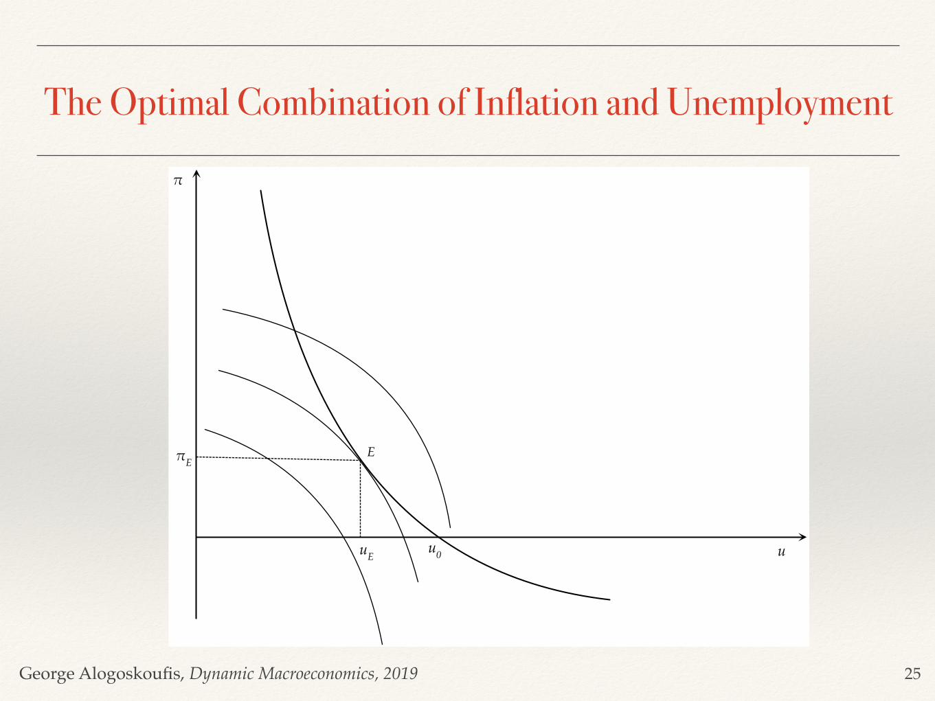
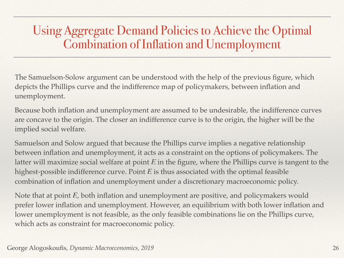
The Samuelson-Solow argument can be understood with the help of the previous figure, which depicts the Phillips curve and the indifference map of policymakers, between inflation and unemployment.

Because both inflation and unemployment are assumed to be undesirable, the indifference curves are concave to the origin. The closer an indifference curve is to the origin, the higher will be the implied social welfare.

Samuelson and Solow argued that because the Phillips curve implies a negative relationship between inflation and unemployment, it acts as a constraint on the options of policymakers. The latter will maximize social welfare at point in the figure, where the Phillips curve is tangent to the highest-possible indifference curve. Point is thus associated with the optimal feasible combination of inflation and unemployment under a discretionary macroeconomic policy.

Note that at point , both inflation and unemployment are positive, and policymakers would prefer lower inflation and unemployment. However, an equilibrium with both lower inflation and lower unemployment is not feasible, as the only feasible combinations lie on the Phillips curve, which acts as constraint for macroeconomic policy.

EE

E

26


Instability of the Phillips Curve and Inflationary Expectations

Since the mid-1960s, the negative relationship between inflation and unemployment began to shift. Higher inflation led to a reduction of unemployment only temporarily, because unemployment rose after a while to return to its original level without a reduction in inflation. This puzzle was soon attributed to shifts in inflationary expectations.

As argued by Phelps (1967) and Friedman (1968), a sustained increase in inflation would lead to expectations of higher future inflation on the part of households and firms. The result of this would be that inflation would have to increase even further in order to achieve a reduction in unemployment. Essentially, Phelps and Friedman argued that the Phillips curve has the form,

where and , and is expected inflation.

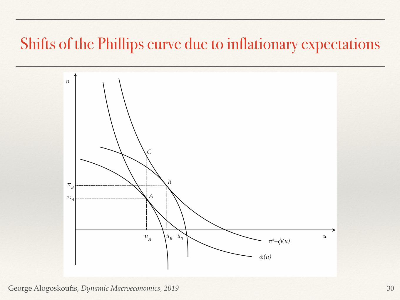
A shift of the Phillips curve due to an increase in inflationary expectations is shown in the figure on the next slide. Assume that initially, inflation and inflationary expectations are equal to zero and unemployment is at . The government and the monetary authorities choose to increase aggregate demand to reduce unemployment, and the economy moves to point , where unemployment has fallen, but inflation has increased. As inflationary expectations gradually adjust to the higher inflation, the Phillips curve moves up, and, thus the economy moves gradually toward point . Inflation rises above at the unemployment rate . Point is no longer feasible. If the government and the monetary authorities want to maximize social welfare they have to adjust monetary and fiscal policy to move the economy to point , which implies higher inflation and unemployment relative to . This would again be temporary, because it would lead to a further gradual upward adjustment in inflationary expectations, a further shift in the Phillips curve, and a further increase in inflation and unemployment.

π = πe + φ(u)

φ(u0) = π − πe = 0 φ′�(u) < 0 πe

u0A

C πAuA A

BA

27


Friedman, Milton (1912-2006)Milton Friedman was an American economist who received the 1976 Nobel Memorial Prize in Economic Sciences for his research on consumption analysis, monetary history and theory and the complexity of stabilization policy.

Friedman's challenges to what he later called "naive Keynesian" theory began with his 1950s reinterpretation of the consumption function. In the 1960s, he became the main advocate opposing Keynesian government policies.

He theorized that there existed a "natural" rate of unemployment and argued that unemployment below this rate would cause inflation to accelerate. He argued that the Phillips curve was in the long run vertical at the "natural rate" and predicted what would come to be known as stagflation.

He promoted an alternative macroeconomic viewpoint known as "monetarism" and argued that a steady, small expansion of the money supply was the preferred policy.

28


Phelps, Edmund Strother (1933-)Phelps is an American economist, a Professor at Columbia University and the recipient of the 2006 Nobel Memorial Prize in Economic Sciences.

His demonstration of the golden rule savings rate, a concept related to work by John von Neumann, started a wave of research on how much a nation should spend on present consumption rather than save and invest for future generations.

His most seminal work concerned the microfoundations of macroeconomics, featuring imperfect information, incomplete knowledge and expectations about wages and prices, to support a macroeconomic theory of employment determination and price-wage dynamics. That led to his development of the natural rate of unemployment: its existence and the mechanism governing its size.

29


Shifts of the Phillips curve due to inflationary expectations

30

!

uu0

φ(u)

!e+φ(u)

Β

Α

uA

!A

uΒ

!Β

C


The Natural Rate of Unemployment and Aggregate Demand Policies

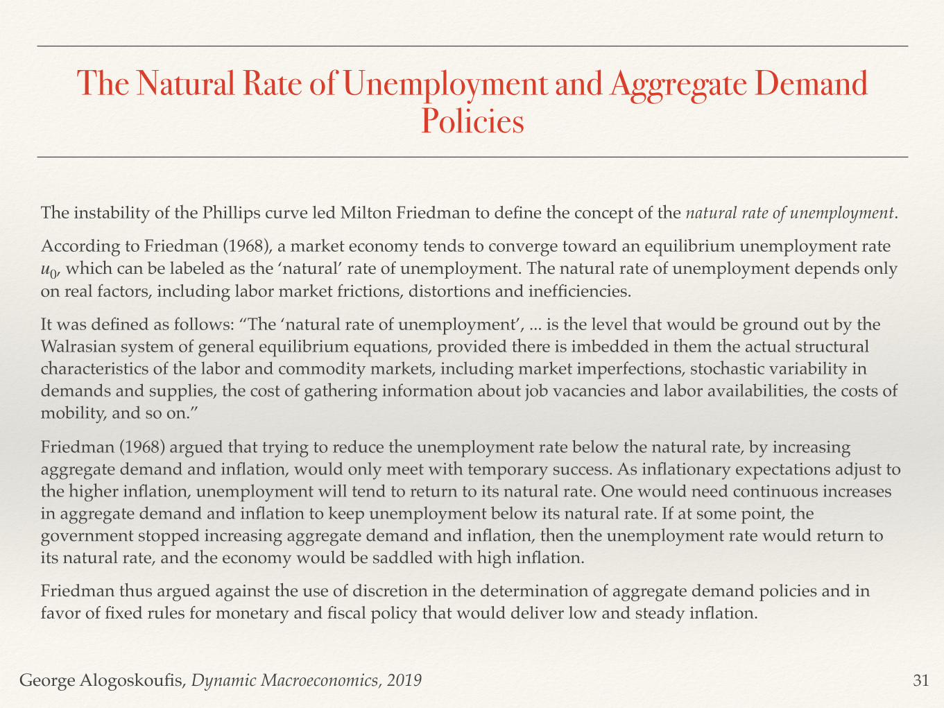
The instability of the Phillips curve led Milton Friedman to define the concept of the natural rate of unemployment.

According to Friedman (1968), a market economy tends to converge toward an equilibrium unemployment rate , which can be labeled as the ‘natural’ rate of unemployment. The natural rate of unemployment depends only

on real factors, including labor market frictions, distortions and inefficiencies.

It was defined as follows: “The ‘natural rate of unemployment’, ... is the level that would be ground out by the Walrasian system of general equilibrium equations, provided there is imbedded in them the actual structural characteristics of the labor and commodity markets, including market imperfections, stochastic variability in demands and supplies, the cost of gathering information about job vacancies and labor availabilities, the costs of mobility, and so on.”

Friedman (1968) argued that trying to reduce the unemployment rate below the natural rate, by increasing aggregate demand and inflation, would only meet with temporary success. As inflationary expectations adjust to the higher inflation, unemployment will tend to return to its natural rate. One would need continuous increases in aggregate demand and inflation to keep unemployment below its natural rate. If at some point, the government stopped increasing aggregate demand and inflation, then the unemployment rate would return to its natural rate, and the economy would be saddled with high inflation.

Friedman thus argued against the use of discretion in the determination of aggregate demand policies and in favor of fixed rules for monetary and fiscal policy that would deliver low and steady inflation.

u0

31


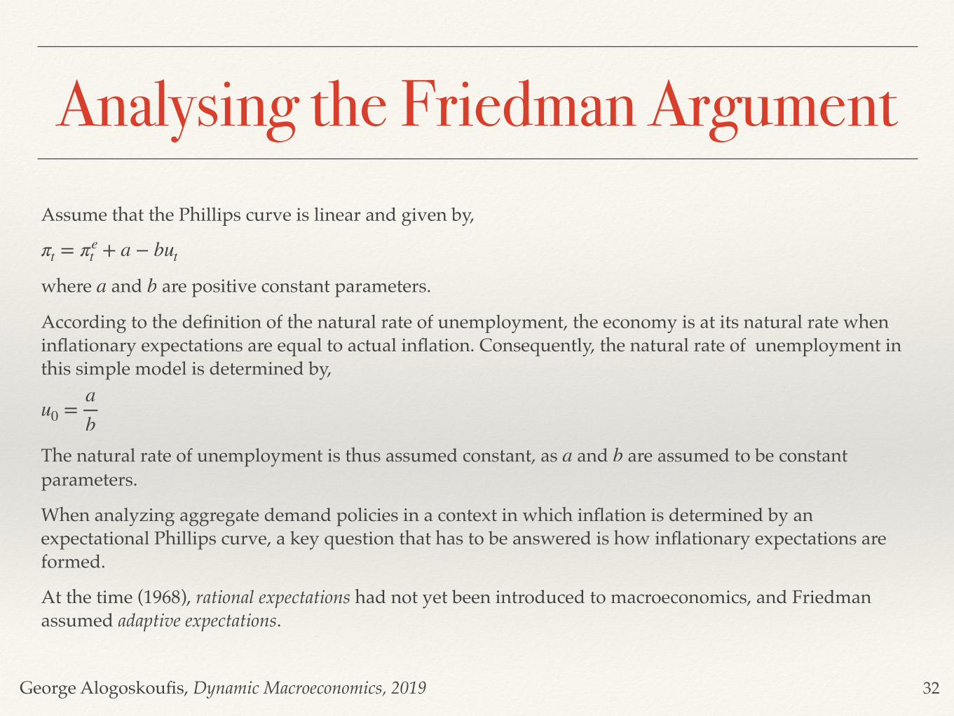
Analysing the Friedman ArgumentAssume that the Phillips curve is linear and given by,

where and are positive constant parameters.

According to the definition of the natural rate of unemployment, the economy is at its natural rate when inflationary expectations are equal to actual inflation. Consequently, the natural rate of unemployment in this simple model is determined by,

The natural rate of unemployment is thus assumed constant, as and are assumed to be constant parameters.

When analyzing aggregate demand policies in a context in which inflation is determined by an expectational Phillips curve, a key question that has to be answered is how inflationary expectations are formed.

At the time (1968), rational expectations had not yet been introduced to macroeconomics, and Friedman assumed adaptive expectations.

πt = πet + a − but

a b

u0 =ab

a b

32


The Path of Inflation and Unemployment under Adaptive Expectations

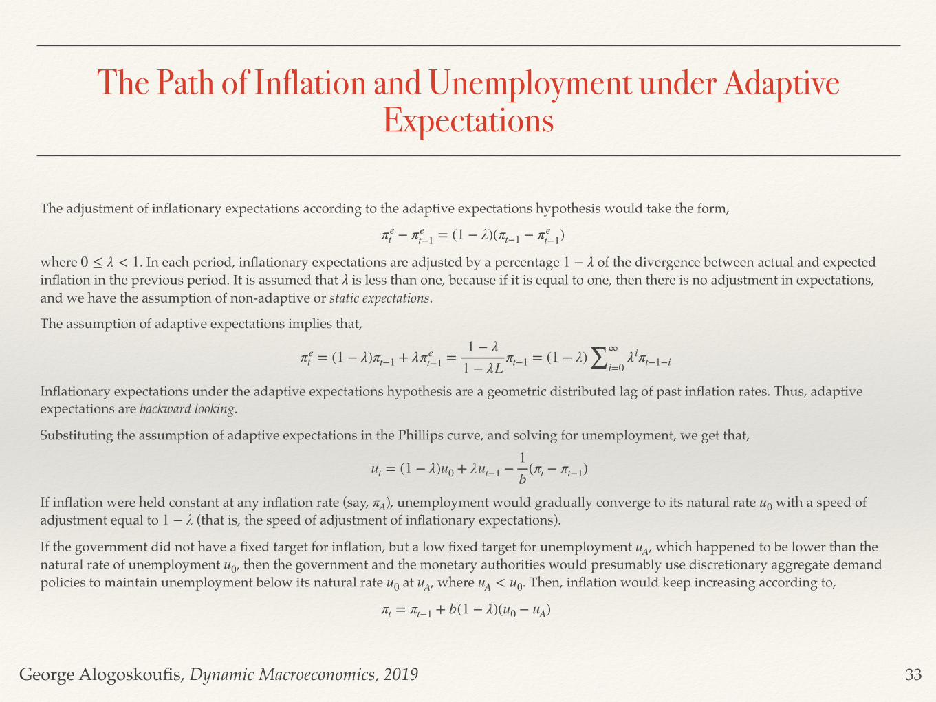
The adjustment of inflationary expectations according to the adaptive expectations hypothesis would take the form,

where . In each period, inflationary expectations are adjusted by a percentage of the divergence between actual and expected inflation in the previous period. It is assumed that is less than one, because if it is equal to one, then there is no adjustment in expectations, and we have the assumption of non-adaptive or static expectations.

The assumption of adaptive expectations implies that,

Inflationary expectations under the adaptive expectations hypothesis are a geometric distributed lag of past inflation rates. Thus, adaptive expectations are backward looking.

Substituting the assumption of adaptive expectations in the Phillips curve, and solving for unemployment, we get that,

If inflation were held constant at any inflation rate (say, ), unemployment would gradually converge to its natural rate with a speed of adjustment equal to (that is, the speed of adjustment of inflationary expectations).

If the government did not have a fixed target for inflation, but a low fixed target for unemployment , which happened to be lower than the natural rate of unemployment , then the government and the monetary authorities would presumably use discretionary aggregate demand policies to maintain unemployment below its natural rate at , where . Then, inflation would keep increasing according to,

πet − πe

t−1 = (1 − λ)(πt−1 − πet−1)

0 ≤ λ < 1 1 − λλ

πet = (1 − λ)πt−1 + λπe

t−1 =1 − λ

1 − λLπt−1 = (1 − λ)∑

∞

i=0λiπt−1−i

ut = (1 − λ)u0 + λut−1 −1b

(πt − πt−1)

πA u01 − λ

uAu0

u0 uA uA < u0

πt = πt−1 + b(1 − λ)(u0 − uA)

33


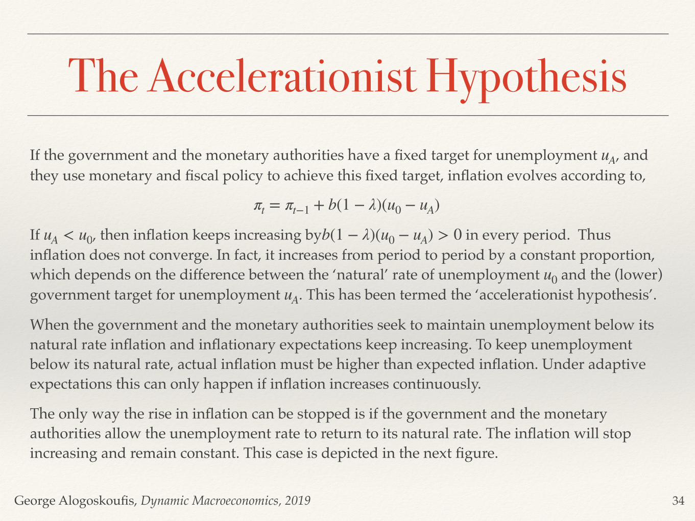
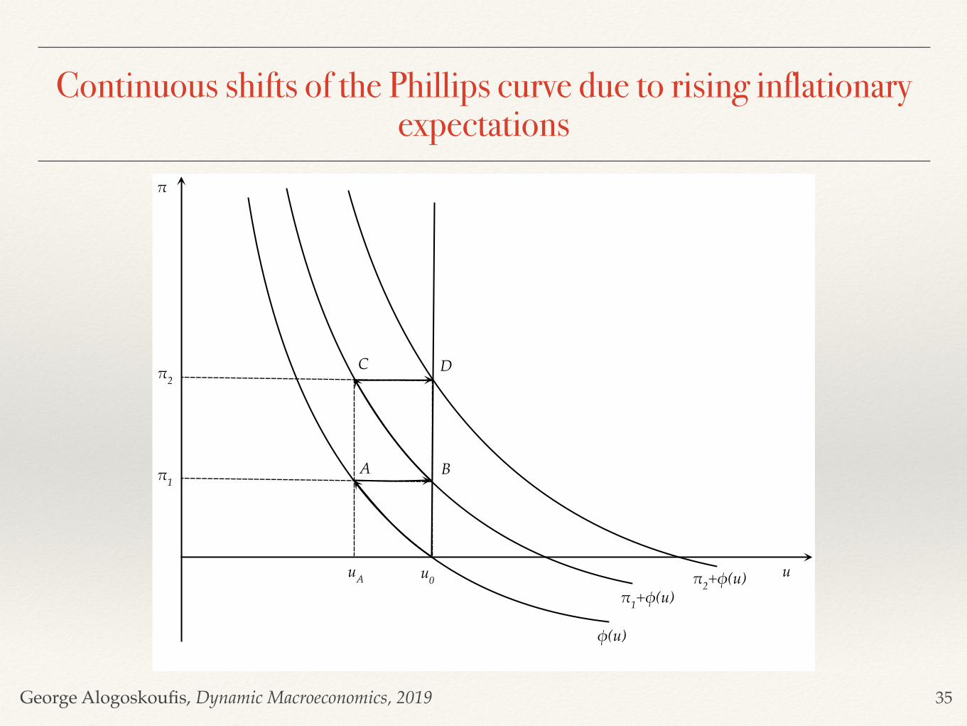
The Accelerationist HypothesisIf the government and the monetary authorities have a fixed target for unemployment , and they use monetary and fiscal policy to achieve this fixed target, inflation evolves according to,

If , then inflation keeps increasing by in every period. Thus inflation does not converge. In fact, it increases from period to period by a constant proportion, which depends on the difference between the ‘natural’ rate of unemployment and the (lower) government target for unemployment . This has been termed the ‘accelerationist hypothesis’.

When the government and the monetary authorities seek to maintain unemployment below its natural rate inflation and inflationary expectations keep increasing. To keep unemployment below its natural rate, actual inflation must be higher than expected inflation. Under adaptive expectations this can only happen if inflation increases continuously.

The only way the rise in inflation can be stopped is if the government and the monetary authorities allow the unemployment rate to return to its natural rate. The inflation will stop increasing and remain constant. This case is depicted in the next figure.

uA

πt = πt−1 + b(1 − λ)(u0 − uA)

uA < u0 b(1 − λ)(u0 − uA) > 0

u0uA

34


Continuous shifts of the Phillips curve due to rising inflationary expectations

35

!

uu0

φ(u)

!1+φ(u)

BA

uA

C D

!1

!2

!2+φ(u)


Inflation and Unemployment under an Optimal Discretionary Policy

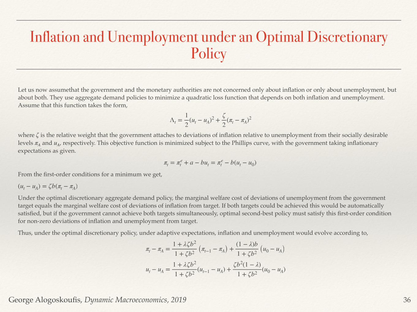
Let us now assumethat the government and the monetary authorities are not concerned only about inflation or only about unemployment, but about both. They use aggregate demand policies to minimize a quadratic loss function that depends on both inflation and unemployment. Assume that this function takes the form,

where is the relative weight that the government attaches to deviations of inflation relative to unemployment from their socially desirable levels and , respectively. This objective function is minimized subject to the Phillips curve, with the government taking inflationary expectations as given.

From the first-order conditions for a minimum we get,

Under the optimal discretionary aggregate demand policy, the marginal welfare cost of deviations of unemployment from the government target equals the marginal welfare cost of deviations of inflation from target. If both targets could be achieved this would be automatically satisfied, but if the government cannot achieve both targets simultaneously, optimal second-best policy must satisfy this first-order condition for non-zero deviations of inflation and unemployment from target.

Thus, under the optimal discretionary policy, under adaptive expectations, inflation and unemployment would evolve according to,

Λt =12

(ut − uA)2 +ζ2

(πt − πA)2

ζπA uA

πt = πet + a − but = πe

t − b(ut − u0)

(ut − uA) = ζb(πt − πA)

πt − πA =1 + λζb2

1 + ζb2 (πt−1 − πA) +(1 − λ)b1 + ζb2 (u0 − uA)

ut − uA =1 + λζb2

1 + ζb2(ut−1 − uA) +

ζb2(1 − λ)1 + ζb2

(u0 − uA)

36


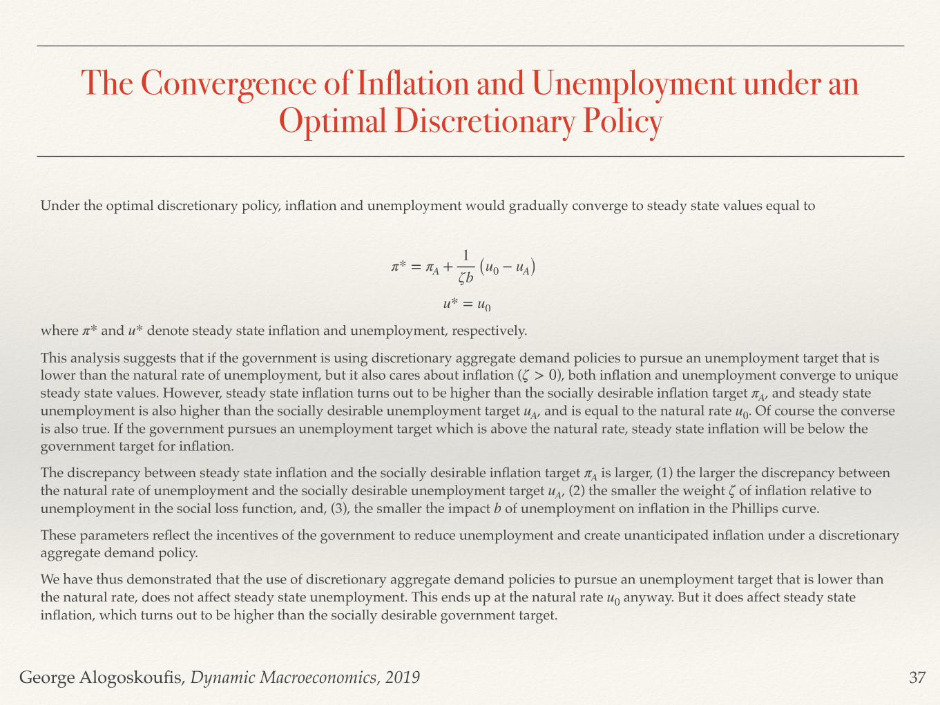
The Convergence of Inflation and Unemployment under an Optimal Discretionary Policy

Under the optimal discretionary policy, inflation and unemployment would gradually converge to steady state values equal to

where and denote steady state inflation and unemployment, respectively.

This analysis suggests that if the government is using discretionary aggregate demand policies to pursue an unemployment target that is lower than the natural rate of unemployment, but it also cares about inflation ( ), both inflation and unemployment converge to unique steady state values. However, steady state inflation turns out to be higher than the socially desirable inflation target , and steady state unemployment is also higher than the socially desirable unemployment target , and is equal to the natural rate . Of course the converse is also true. If the government pursues an unemployment target which is above the natural rate, steady state inflation will be below the government target for inflation.

The discrepancy between steady state inflation and the socially desirable inflation target is larger, (1) the larger the discrepancy between the natural rate of unemployment and the socially desirable unemployment target , (2) the smaller the weight of inflation relative to unemployment in the social loss function, and, (3), the smaller the impact of unemployment on inflation in the Phillips curve.

These parameters reflect the incentives of the government to reduce unemployment and create unanticipated inflation under a discretionary aggregate demand policy.

We have thus demonstrated that the use of discretionary aggregate demand policies to pursue an unemployment target that is lower than the natural rate, does not affect steady state unemployment. This ends up at the natural rate anyway. But it does affect steady state inflation, which turns out to be higher than the socially desirable government target.

π* = πA +1ζb (u0 − uA)

u* = u0

π* u*

ζ > 0πA

uA u0

πAuA ζ

b

u0

37


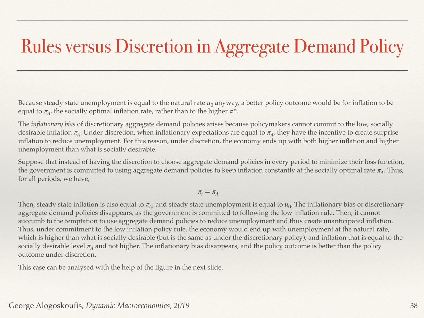
Rules versus Discretion in Aggregate Demand Policy

Because steady state unemployment is equal to the natural rate anyway, a better policy outcome would be for inflation to be equal to , the socially optimal inflation rate, rather than to the higher .

The inflationary bias of discretionary aggregate demand policies arises because policymakers cannot commit to the low, socially desirable inflation . Under discretion, when inflationary expectations are equal to , they have the incentive to create surprise inflation to reduce unemployment. For this reason, under discretion, the economy ends up with both higher inflation and higher unemployment than what is socially desirable.

Suppose that instead of having the discretion to choose aggregate demand policies in every period to minimize their loss function, the government is committed to using aggregate demand policies to keep inflation constantly at the socially optimal rate . Thus, for all periods, we have,

Then, steady state inflation is also equal to , and steady state unemployment is equal to . The inflationary bias of discretionary aggregate demand policies disappears, as the government is committed to following the low inflation rule. Then, it cannot succumb to the temptation to use aggregate demand policies to reduce unemployment and thus create unanticipated inflation. Thus, under commitment to the low inflation policy rule, the economy would end up with unemployment at the natural rate, which is higher than what is socially desirable (but is the same as under the discretionary policy), and inflation that is equal to the socially desirable level and not higher. The inflationary bias disappears, and the policy outcome is better than the policy outcome under discretion.

This case can be analysed with the help of the figure in the next slide.

u0πA π*

πA πA

πA

πt = πA

πA u0

πA

38


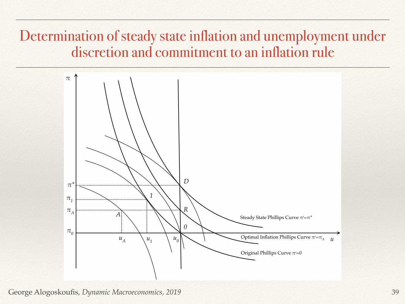
Determination of steady state inflation and unemployment under discretion and commitment to an inflation rule

39

!

uu0u1

1!1!A

uA

A

0!0

!*

Original Phillips Curve !e=0

Steady State Phillips Curve !e=!*

D

R

Optimal Inflation Phillips Curve !e=!A


Analysis of the Time Inconsistency of Optimal Policy

Assume that originally, the economy is at the natural rate of unemployment, with zero inflation (point 0). The government decides to expand aggregate demand to reduce unemployment. This has the effect of increasing inflation along the original Phillips curve. The economy ends up at point 1, where the original Phillips curve is tangent to the highest possible social indifference curve between inflation and unemployment. Point 1 implies lower unemployment and higher inflation. In the short run, the government is better off, as the welfare loss associated with point 1 is lower than that associated with point 0. Note that point A, which implies the lowest-possible welfare loss cannot be attained. But point 1 is not a stable equilibrium, because inflationary expectations start adapting to the higher inflation , and the Phillips curve starts shifting upward.

Thus, the government will need to further increase aggregate demand to keep unemployment below the natural rate. This will generate a further increase in inflation, further upward revisions of inflationary expectations, and so on.

The process will only stop when the economy ends up at point (for ‘discretion’), and expectations adapt to the inflation rate . At point the government no longer has an incentive to further expand aggregate demand to reduce unemployment. The welfare costs from further increases in inflation exceed the welfare benefits from the reduction in unemployment. Thus, is a stable steady state equilibrium.

Under commitment to an inflation rule that keeps inflation equal to , the economy converges to the steady state equilibrium (for ‘rules’). is preferable to , because it is associated with lower steady state inflation ( ) and the same unemployment rate. The problem is that at

, the government has a short-run incentive to renege on its commitment and expand aggregate demand to reduce unemployment. The short-run marginal welfare gain from the reduction in unemployment is higher than the short-run marginal welfare loss from the rise in inflation. Thus, the commitment mechanism must be binding for the government not to succumb to the temptation of increasing aggregate demand.

These results were first demonstrated by KydlandPrescott (1977), under the assumption of rational expectations. As we have demonstrated in this section, they hold in the steady state under adaptive expectations too. The discretionary (time-consistent) policy is not intertemporally optimal, in the sense that there is a better policy outcome under commitment to the low inflation rule. However, the low inflation rule is not time consistent, because the government has an incentive to deviate from it in every period. Thus, the intertemporally optimal steady state policy rule is time inconsistent: it is not optimal in the short run.

π1

D π* D

D

πA R RD πA < π*

R

40


Inflation and Unemployment under Rational Expectations

Our analysis so far has been based on the assumption of adaptive expectations. One of the consequences of the realization that the original Phillips curve is unstable was the adoption of the hypothesis of rational expectations. The hypothesis of rational expectations gradually became the key hypothesis regarding the formation of expectations, not only about inflation, but about all future variables that affect the behavior of households and firms, as well as governments.

In this particular context, rational expectations implies that households and firms form inflationary expectations that take into account the incentives of governments to use discretionary policies to choose between inflation and unemployment. It is thus worth analyzing the implications of the rational expectations hypothesis for this model of the natural rate.

From the first-order conditions for a minimum of the government social loss function subject to the Phillips curve, we get that under discretionary policies inflation and unemployment must satisfy,

Because there are no stochastic disturbances, the hypothesis of rational expectations implies that expected and actual inflation will coincide. Thus, combined with the rational expectations hypothesis, the above equation implies that

Under rational expectations, in the absence of stochastic disturbances, inflation is always equal to expected inflation. Thus, inflation jumps to steady state inflation immediately. Consequently, unemployment also jumps to its natural rate immediately. Discretionary aggregate demand policies cannot affect unemployment even in the short run, and they only result in both short-run and steady state inflationary bias, because of the incentives of the government to create surprise inflation and the immediate adjustment of expectations to anticipate these incentives.

In contrast, under commitment to the time inconsistent policy rule inflation is equal to and the unemployment rate is equal to the natural rate in all periods. The argument in favour of commitment to rules is even stronger.

(u0 − uA −1b

(πt − πet ) = ζb(πt − πA)

πt = πet = πA +

1ζb

(u0 − uA)

πt = πet = πA

u0

41


ConclusionsWe have seen that what separates classical from Keynesian models is the assumption of nominal rigidity or gradual adjustment in nominal wages and the price level. We have looked at the structure of the basic Keynesian models, assuming initially a constant level of prices or nominal wages, and then gradual adjustment of prices and nominal wages, based on the Phillips curve. We also explored the theory of discretionary aggregate demand policy that was originally developed on the basis of these models.

According to the basic Keynesian model, combined with the Phillips curve, an increase in aggregate demand - either through government expenditure (or a tax cut) or through an increase in the money supply - leads to an increase in real income and employment, a reduction of unemployment, and increased inflation. Conversely, a decline in aggregate demand leads to a decline of real income and employment, an increase in unemployment and reduced inflation. As argued by Samuelson and Solow (1960), the short-term objective of macroeconomic policy can be seen as the appropriate selection of a discretionary mix of monetary and fiscal policies that would deliver the desired combination of unemployment and inflation. Thus, the adoption of the Keynesian approach led to a shift toward discretion in the determination of monetary and fiscal policies.

The instability of the original Phillips curve observed in the late 1960s, and the interpretation given to this instability by Phelps (1967) and Friedman (1968), have since sparked a revolution in the analysis of aggregate fluctuations and the evaluation of aggregate demand policies.

The literature has since moved in three directions. First, great emphasis was placed on the microeconomic foundations of the determination of wages, prices, the supply and demand for goods and services, and the determination of the equilibrium unemployment rate. The result is that today both the new classical and the new keynesian approaches to aggregate fluctuations are based on DSGE models with consistent dynamic microeconomic foundations.

Second, the instability of the original Phillips curve eventually led to the adoption of the hypothesis of rational expectations: the hypothesis that households and firms form inflationary expectations that take into account the motives of governments and central banks to choose between inflation and unemployment.

Third, the debate on the appropriate use of monetary and fiscal policy has shifted in favor of rules rather than discretion. The problem of macroeconomic policy design is no longer a question of rules versus discretion, but a question of the appropriate design of policy rules.

42

Documents

Athens University of Economics and Business Dynamic ... · The Distinguishing Feature of the Keynesian Approach In the Keynesian models, the immediate adjustment of prices and wages