Draft version October 3, 2018Preprint typeset using LATEX style AASTeX6 v. 1.0

FAR-INFRARED TO MILLIMETER DATA OF PROTOPLANETARY DISKS: DUST GROWTH IN THE

TAURUS, OPHIUCHUS, AND CHAMAELEON I STAR-FORMING REGIONS∗.

Alvaro Ribas1, Catherine C. Espaillat1, Enrique Macıas1, Herve Bouy2, Sean Andrews3, Nuria Calvet4, DavidA. Naylor5, Pablo Riviere-Marichalar6, Matthijs H. D. van der Wiel5, 7, and David Wilner3

1Department of Astronomy, Boston University, Boston, MA 02215, USA; aribas@bu.edu2Laboratoire d’Astrophysique de Bordeaux, Univ. Bordeaux, CNRS, F-33615 Pessac, France3Harvard-Smithsonian Center for Astrophysics, Cambridge, MA 91023 USA4Astronomy Department, University of Michigan, Ann Arbor, MI 48109, USA5Institute for Space Imaging Science, Department of Physics & Astronomy, University of Lethbridge, Canada6Instituto de Ciencia de Materiales de Madrid (CSIC). Calle Sor Juana Ines de la Cruz 3, E-28049 Cantoblanco, Madrid, Spain7ASTRON, the Netherlands Institute for Radio Astronomy, PO Box 2, 7990AA Dwingeloo, The Netherlands

ABSTRACT

Far-infrared and (sub)millimeter fluxes can be used to study dust in protoplanetary disks, the building

blocks of planets. Here, we combine observations from the Herschel Space Observatory with ancillary

data of 284 protoplanetary disks in the Taurus, Chamaeleon I, and Ophiuchus star-forming regions,

covering from the optical to mm/cm wavelengths. We analyze their spectral indices as a function of

wavelength and determine their (sub)millimeter slopes when possible. Most disks display observational

evidence of grain growth, in agreement with previous studies. No correlation is found between other

tracers of disk evolution and the millimeter spectral indices. A simple disk model is used to fit

these sources, and we derive posterior distributions for the optical depth at 1.3 mm and 10 au, the

disk temperature at this same radius, and the dust opacity spectral index β. We find the fluxes at

70µm to correlate strongly with disk temperatures at 10 au, as derived from these simple models.

We find tentative evidence for spectral indices in Chamaeleon I being steeper than those of disks

in Taurus/Ophiuchus, although more millimeter observations are needed to confirm this trend and

identify its possible origin. Additionally, we determine the median spectral energy distribution of each

region and find them to be similar across the entire wavelength range studied, possibly due to the

large scatter in disk properties and morphologies.

Keywords: protoplanetary disks — stars: pre-main sequence — infrared: general — submillimeter:

general

1. INTRODUCTION

Planetary systems form out of disks of gas and dust

around young stars. However, the large number of

physical processes taking place within them (e.g., ac-

cretion, photoevaporation, interaction with companions,

dust growth and settling, radial migration, Takeuchi &

Lin 2002; D’Alessio et al. 2006; Ireland & Kraus 2008;

Alexander et al. 2014) require that we consider sev-

eral factors for their study. For this purpose, multi-

wavelength observations of protoplanetary disks can be

used to better understand their properties.

The (sub)mm wavelength range is of particular inter-

*Herschel is an ESA space observatory with science instrumentsprovided by European-led Principal Investigator consortia andwith important participation from NASA.

est for various reasons: at sufficiently long wavelengths,

disks become optically thin, and an estimate of their

dust mass can be directly obtained (via some assump-

tions) by simply measuring their flux (e.g. Beckwith

et al. 1990). Although the bulk of the disk mass in the

system is in gaseous phase, fiducial (or measured, when

available) gas-to-dust ratios provide an indirect estimate

of the total mass in the disk. This is a crucial parameter

for planet formation theories because it determines the

available reservoir for this process. Using this method,

surveys of star-forming regions with (sub)mm facilities

such as SMA and ALMA have determined that proto-

planetary disks have typical masses of 0.1-0.5 % of that

of their host star (e.g. Andrews & Williams 2005; An-

drews et al. 2013; Pascucci et al. 2016). On the other

hand, dust growth represents the initial stage of planet

formation; the observed spectral index at these wave-

arX

iv:1

710.

0842

6v1

[as

tro-

ph.S

R]

23

Oct

201

7

2 Ribas et al. 2017

lengths can be linked to the dust opacity in the disk,

informative of its properties and grain sizes (e.g. Miyake

& Nakagawa 1993; Draine 2006). In fact, the compar-

ison of the millimeter spectral index of the interstellar

medium (ISM) with that of protoplanetary disks has

already revealed significant dust growth in these disks,

implying the presence of mm/cm-sized grains in many

of them (e.g. D’Alessio et al. 2001; Lommen et al. 2010;

Ricci et al. 2010b,a; Ubach et al. 2012). The combina-

tion of the mm spectral index with additional informa-

tion at other wavelengths, such as the spectral index at

near/mid infrared (IR) wavelengths or silicate features

may also point to links between the evolution of the

inner and outer regions of the disks. As an example,

Lommen et al. (2010) identified a tentative correlation

between the strength of the 10µm silicate feature and

the 1-3 mm spectral index for a sample of T Tauri and

Herbig Ae/Be stars, suggesting a connection between

the evolution of the inner and outer regions of disks, al-

though a later study by Ricci et al. (2010a) found no

signs of such a correlation for disks in the Taurus and

Ophiuchus star-forming regions. Despite the obvious in-

terest of this wavelength regime, disks have relatively

weak emission at millimeter wavelengths and many of

them currently lack this type of data (or, at least, suf-

ficient observations to provide robust estimates of their

spectral indices).

At somewhat shorter wavelengths, the Herschel Space

Observatory (Herschel, Pilbratt et al. 2010) observed

large areas of the sky in the far-IR and sub-mm, in-

cluding several star-forming regions (e.g. the Gould

Belt Survey, Andre et al. 2010). Herschel probed the

range between 50 and 150 µm, which is sensitive to

dust settling (e.g. D’Alessio et al. 2006), but also pro-

vided fluxes at longer wavelengths (up to ∼ 700µm)

probing deeper into the disk mid-plane. Various stud-

ies have already analyzed different aspects of Herschel

data in star-forming regions, both from the photometric

(e.g. Winston et al. 2012; Howard et al. 2013; Olofs-

son et al. 2013; Ribas et al. 2013; Spezzi et al. 2013;

Bustamante et al. 2015; Rebollido et al. 2015) and spec-

troscopic (Cieza et al. 2013; Dent et al. 2013; Riviere-

Marichalar et al. 2016) points of view. On the other

hand, a large comparative analysis of Herschel data of

protoplanetary disks in different star-forming regions is

still missing.

In this work, we compile multi-wavelength data of pro-

toplanetary disks, including homogeneous Herschel pho-

tometry and spectroscopy, in three nearby star-forming

region: Taurus (1-2 Myr and ∼140 pc, Torres et al.

2007; Andrews et al. 2013), Ophiuchus (0.3-5 Myr and

∼140 pc, Wilking et al. 2008; Ortiz-Leon et al. 2017),

and Chamaeleon I (2-6 Myr and ∼160 pc, Whittet et al.

1997; Luhman 2007). The proximity of these regions and

the amount of available ancillary data guarantee good

coverage of the spectral energy distributions (SEDs) of

several of their disks. Sec. 2 describes our sample, data

compilation, and processing. In Sec. 3 we analyze differ-

ent aspects of (sub)mm spectral indices and investigate

observational evidence of dust growth in these SEDs. In

Sec. 4, we provide further analysis by fitting the com-

piled data with a simple disk model. Sec. 5 discusses and

compares the median SEDs of these regions. Finally, our

conclusions are presented in Sec. 6.

2. SAMPLE AND DATA COMPILATION

Our goal was to compile a representative sample of

the disk population in the Taurus, Ophiuchus, and

Chamaeleon I molecular clouds, while also ensuring a

good coverage of their SEDs from the optical to the

far-IR, as well as the millimeter range when possible.

We considered the 161 Taurus objects studied by Furlan

et al. (2011), 134 objects in Ophiuchus in McClure et al.

(2010), and the 84 objects in Chamaeleon I analyzed

in Manoj et al. (2011). These studies presented and

analyzed Spitzer/IRS spectra of these disks, and per-

formed a detailed study of the properties of their inner

regions. They also provided homogeneous compilations

of the stellar properties of these objects. Based on this

and our intention to model these sources in more detail

in a future study, we selected these three sub-samples as

our initial sample. To avoid disks with significant con-

tribution from their envelopes, we discarded envelope-

dominated SEDs (as identified in these studies), which

were present both in the Ophiuchus and Chamaeleon I

samples. Our final sample comprises 315 objects: 161

in Taurus, 83 in Ophiuchus, and 71 in Chamaeleon I.

2.1. Herschel data

Due to the different methods used to process Herschel

data in various studies and the inherent difficulties of

obtaining photometric and spectroscopic measurements

in the presence of conspicuous background emission (the

cold dust in molecular clouds emits strongly at far-IR

wavelengths), a coherent comparison of these data is

complex and has not yet been explored. To guarantee a

homogeneous data set, observations of the three regions

were processed in the same manner.

2.1.1. Herschel Photometry

We processed a number of scan and cross scan maps

available in the Herschel Science Archive to achieve a

satisfactory coverage of the three regions considered in

this study. All of them were obtained by the the Her-

schel Gould Belt Survey (P.I.: Philippe Andre), except

for one set of observations in Ophiuchus (P.I.: Peter

Abraham). The corresponding OBSIDs, instruments,

wavelengths, and pointing coordinates are summarized

Disks in Taurus, Ophiuchus, and Chamaeleon I 3

in Table A1 in Appendix A. After this process, a total

number of 18 objects in our sample lie outside the cov-

erage of the large maps used in this study. For these,

we queried the Herschel Science Archive to retrieve ad-

ditional (smaller) observations that contained these ob-

jects. We found PACS detections for 11 of these sources.

The corresponding OBSIDs and information for these

data are also listed in Appendix A.

Maps at the three PACS wavelengths (70, 100, and

160µm) were processed using the JScanam algorithm

(Gracia-Carpio et al. 2015) within HIPE (Herschel In-

teractive Processing Environment, Ott 2010) version 14,

combining scan and cross scan maps. In the particular

case of OBSIDs 1342202254 (scan), 1342202090 (cross

scan 1) and 1342190616 (cross scan 2), these three maps

cover the same region of the sky, but JScanam can only

process scan + cross scan pairs. For this reason, we

produced two different maps with each scan and cross

scan combination. We then extracted PACS aperture

photometry at the nominal coordinates of each object

with the annular sky aperture photometry task within

HIPE, using aperture radii of 15”, 18”, and 22” for 70,

100, and 160µm, respectively. These values were de-

termined to be a good compromise based on inspection

of growth curves obtained in scan + cross scan maps.

The background was estimated within an annulus with

radii of 25” and 35” centered around each object. We

then applied the corresponding aperture correction fac-

tors with the photApertureCorrectionPointSource task,

corresponding to 0.83, 0.84, and 0.82 for 70, 100, and

160µm, respectively. Given the different slopes of Class

II SEDs in the PACS regime, we chose not to apply color

corrections to these fluxes—which, in any case, are sig-

nificantly smaller than the assumed uncertainties (see

below).

SPIRE photometry was obtained at the three avail-

able wavelengths (250, 350, and 500µm) using the rec-

ommended procedure of fitting sources in the timeline

(Pearson et al. 2014) within HIPE. The level 1 data

were previously corrected using the destriper task. No

extended emission gains were applied because we do

not expect any of these disks to be resolved in Her-

schel/SPIRE maps at their corresponding distances.

The timeline fitting method does not require aperture

corrections, but we did apply color corrections in this

case; at the longer SPIRE wavelengths, disks are (at

least partly) optically thin, and their emission at these

wavelengths can therefore be fitted with a power law.

Based on mm spectral indexes by Ricci et al. (2010b),

we used an intermediate power-law index of 2.3 and ap-

plied the corresponding color corrections. The uncer-

tainty from this parameter is, in any case, of only a few

percent1.

Reliable source detection in Herschel maps of star-

forming regions is a challenging task, given the strong

(and usually highly structured) background emission.

We therefore performed visual inspection of each source

in all the available wavelengths to guarantee that we

only include clean point source detections. We dis-

carded every source/band with extended objects, sig-

nificant contribution by nearby sources or the emission

from the molecular clouds, or tentative/non detections.

For objects covered by more than one map, the me-

dian flux value was adopted. To account for the effect

of the aforementioned conspicuous background at Her-

schel wavelengths, based on previous Herschel studies

(e.g. Ribas et al. 2013; Rebollido et al. 2015), we as-

signed a conservative 20 % uncertainty to each Herschel

photometric measurement. The resulting photometry,

together with objects that were discarded during the vi-

sual inspection process, are listed in Appendix B.

2.1.2. Herschel/SPIRE Spectroscopy

We also obtained SPIRE Fourier Transform Spec-

trometer (FTS) low-resolution (λ/4λ = 48 at 250µm)

spectra for 113 objects (P.I.: Catherine Espaillat, pro-

posal ID: OT1 cespaill 1). These data cover wavelengths

from 190 to 670µm, and were processed within HIPE

14 using the standard pipeline (Fulton et al. 2016),

which also reduces the long-wavelength artifacts pro-

duced when operating the SPIRE FTS in low-resolution

mode (Marchili et al. 2017). In addition to standard pro-

cessing, background subtraction is crucial at long wave-

lengths in star-forming regions. We inspected all SPIRE

detectors for each object to discard undetected sources,

and removed those on top of isolated strong background

emission that could yield an overestimation of the true

background flux. Once a reliable estimate of the back-

ground flux was established, it was subtracted from the

detector viewing the source. We applied the pointing

offset correction within HIPE (Valtchanov et al. 2014)

when possible, in order to mitigate discontinuities be-

tween the two spectral windows. The extremities of the

spectra were then trimmed to avoid the lower S/N re-

gions. Finally, the resulting spectra were compared with

SPIRE data and archival photometry (see next section),

and we discarded those with obvious discrepancies with

the photometry, mostly due to decreasing signal to noise

with increasing wavelengths. Thirty-four clean SPIRE

spectra remained after this process, and are available in

the online version. The obsids of both clean and dis-

carded SPIRE FTS spectra are listed in Appendix A.

1 http://herschel.esac.esa.int/Docs/SPIRE/spire handbook.pdf

4 Ribas et al. 2017

Table

1.

Cata

logs

and

Surv

eys

Use

din

this

Stu

dy

Cata

log/Surv

eyT

eles

cop

e/In

stru

men

t(s)

Wav

elen

gth

range

Reg

ion

aR

efer

ence

Slo

an

Dig

ital

Sky

Surv

ey(D

R9)

SD

SS

tele

scop

e0.3

5-

0.9

1µ

m..

.A

hn

etal.

(2012)

AA

VSO

Photo

met

ric

All

Sky

Surv

ey(A

PA

SS)

Mult

iple

tele

scop

es0.4

4-

0.7

6µ

m..

.H

enden

etal.

(2016)

Carl

sber

gM

erid

ian

Cata

log

(DR

15)

CM

T0.6

2µ

m..

...

.

Tw

oM

icro

nA

llSky

surv

ey(2

MA

SS)

2M

ASS

1.2

4-

2.1

6µ

m..

.Skru

tskie

etal.

(2006)

WideInfraredExplorer(W

ISE)

WISE

3.4

-22µ

m..

.W

right

etal.

(2010)

Core

sto

dis

ks

(c2d)

surv

eySpitzer/IR

AC

,M

IPS

3.6

-24µ

mT

auru

s,O

phiu

chus

Eva

ns

etal.

(2009)

AKARI

mid

-infr

are

dsu

rvey

AKARI/IR

C9

-18µ

m..

.Is

hih

ara

etal.

(2010)

-A

LM

A887µ

mT

auru

sR

icci

etal.

(2014)

-IR

AM

Pla

teau

de

Bure

Inte

rfer

om

eter

3.2

mm

Tauru

sP

ietu

etal.

(2014)

-SC

UB

A/JC

MT

+lite

ratu

re350µ

m-

1.3

mm

Ophiu

chus

Andre

ws

&W

illiam

s(2

007)

-A

LM

A890µ

mO

phiu

chus

Tes

tiet

al.

(2016)

-A

TC

A3.3

mm

Ophiu

chus

Ric

ciet

al.

(2010a)

-V

LA

4-

7cm

Ophiu

chus

Dzi

bet

al.

(2013)

-Spitzer/IR

AC

,M

IPS

3.4

-24µ

mC

ham

ael

eon

IL

uhm

an

etal.

(2008)

-SE

ST

1.3

mm

Cham

ael

eon

IH

ennin

get

al.

(1993)

-A

PE

X/L

AB

OC

A870µ

mC

ham

ael

eon

IB

ello

che

etal.

(2011)

-A

LM

A887µ

mC

ham

ael

eon

IP

asc

ucc

iet

al.

(2016)

-A

TC

A3

mm

-6

cmC

ham

ael

eon

IU

bach

etal.

(2012)

aO

nly

for

regio

n-s

pec

ific

surv

eys.

Note—

The

majo

rity

of

the

data

for

Tauru

sob

ject

sw

ere

gath

ered

from

the

com

pilati

on

inA

ndre

ws

etal.

(2013),

and

we

refe

rth

ere

ader

toth

isst

udy

for

addit

ional

info

rmati

on.

Disks in Taurus, Ophiuchus, and Chamaeleon I 5

2.2. Archival data

To complement Herschel data, we queried a number

of catalogs for photometry covering a broad wavelength

range. In the case of Taurus, data from the compre-

hensive compilation by Andrews et al. (2013) was used

when available. Ancillary photometry in the range of

60-160µm was found to be significantly noisy (possi-

bly due to the lower resolution and sensitivity of pre-

vious facilities/telescopes), and was excluded because

Herschel data are now available. For the remaining Tau-

rus objects, as well as for Ophiuchus and Chamaeleon,

we cross-matched our sample with a number of surveys

and catalogs, listed in Table 1. The cross-match was

performed by assigning the fluxes to the closest source

within a radius of 3′′, except for APEX/LABOCA,

SCUBA, or VLA, where a 5′′search radius was used due

to their larger beam sizes.

We paid special attention to saturation magnitudes

and the various flags (such as objects marked as ex-

tended) in different observations. It is likely that some

of the compiled data suffer from undetected additional

problems (e.g., contamination by nearby sources) that

may affect our analysis, particularly in the (sub)mm do-

main; we therefore inspected each SED visually and dis-

carded any photometric point clearly inconsistent with

the overall shape of the SED. This process also helps to

identify and discard possible missmatches in the cross-

matching process.

Spitzer/IRS (Houck et al. 2004) spectra of these ob-

jects were also retrieved from the Cornell Atlas of

Spitzer/IRS Sources (CASSIS, Lebouteiller et al. 2011,

2015). CASSIS produces optimally extracted spectra

(accounting for e.g. pointing shifts in the slit, local back-

ground), which are suitable for our purposes. However,

for some sources, we find issues in the automatic reduc-

tion by CASSIS (e.g. non-matching orders); in those

cases we used the spectra from Furlan et al. (2011), Mc-

Clure et al. (2010), and Manoj et al. (2011). If sev-

eral spectra were available in CASSIS, we visually in-

spected them and chose those that better matched our

compiled photometry, given that the mid-IR emission of

disks can be variable (e.g. Espaillat et al. 2011; Morales-

Calderon et al. 2011). Furthermore, we do not include

the spectrum for T Tau, given the strong neighboring

background emission and its inconsistency with the com-

piled SED.

To our knowledge, this is the largest data compilation

to date for Chamaeleon I and Ophiuchus. An example of

one of the compiled, clean SEDs is presented in Table 2.

The whole data set (SEDs and available SPIRE and IRS

spectra) is available for download in tar.gz packages. In

addition, the entire data set is available in a Zenodo

archive [10.5281/zenodo.889053].

Table 2. Example of One of the Observed (Not De-

reddened) SEDsa: WX Cha

Wavelength Fν Reference

(µm) (mJy)

0.44 4.5±0.9 Henden et al. (2016)

0.48 6±1 Henden et al. (2016)

0.55 11±2 Henden et al. (2016)

0.62 19±4 Henden et al. (2016)

0.76 35±4 Henden et al. (2016)

1.23 186±5 Skrutskie et al. (2006)

1.66 320±10 Skrutskie et al. (2006)

2.16 432±7 Skrutskie et al. (2006)

3.6 450±20 Luhman et al. (2008)

4.5 450±20 Luhman et al. (2008)

4.6 430±10 Wright et al. (2010)

5.8 400±20 Luhman et al. (2008)

8.0 400±20 Luhman et al. (2008)

9.0 440±20 Murakami et al. (2007)

12 370±20 Wright et al. (2010)

18 420±30 Murakami et al. (2007)

22 410±20 Wright et al. (2010)

24 390±20 Luhman et al. (2008)

70 330±70 This work

100 220±40 This work

160 180±40 This work

160 120±20 This work

250 100±20 This work

350 110±20 This work

500 120±20 This work

887 21±2 Pascucci et al. (2016)

aThe IRS spectrum is available in the online version ofthe manuscript.

Note—Similar datasets, including Spitzer/IRS andHerschel/SPIRE spectra are available for each ofthe considered sources in the online version of themanuscript.

2.3. De-reddening and stellar parameters

The data were de-reddened using AV values for Ophi-

uchus (McClure et al. 2010) and AJ values for Tau-

rus and Chamaeleon I (Furlan et al. 2011; Manoj et al.

2011). We followed the procedure adopted in McClure

et al. (2010) to select the extinction law to be used for

each target:

1. For AV < 3, we use the extinction law in Mathis

(1990) with RV =3.1.

6 Ribas et al. 2017

10000 2000300040006000

Teff [K]

10−3

10−1

101

103L∗[

L�

]

Taurus

Chamaeleon

Ophiuchus

1 Myr

3 Myr

10 Myr

100 Myr

Figure 1. HR diagram of the sample. Taurus objectsare shown as red circles, Chamaeleon as yellow squares,and Ophiuchus members as blue triangles. Underluminoussources are likely YSOs with edge-on disks, self-extinctingtheir stellar radiation. Isochrones from Baraffe et al. (2015)are also shown for comparison.

2. For cases 3 ≤ AV < 8 and AV > 8, we use the cor-

responding the extinction laws in McClure (2009).

In the following, sources with AV ≥ 15 are excluded

from the analysis: these objects are either highly embed-

ded in their parental cloud or located behind a signifi-

cant amount of dust. In both cases, their spectral types

(SpTs) are more uncertain, and such large extinctions

may create important features in the SED shape that

could alter the result of our analysis. Moreover, the ob-

scuring dust will emit at longer wavelengths (longward

of far-IR), and both Herschel photometry and ancillary

data may be contaminated by this emission. After this

stage of the analysis, the sample size has been reduced

to 284 YSOs: 154 in Taurus, 70 in Ophiuchus, and 60

in Chamaeleon I.

To assign stellar parameters, we used SpTs listed in

Furlan et al. (2011), McClure et al. (2010), and Manoj

et al. (2011). These were translated into stellar effective

temperatures (Teff) using the updated SpT–Teff relation

in Pecaut & Mamajek (2013). We then scaled the cor-

responding BT-Settl photospheres (Allard et al. 2012)

to the de-reddened 2MASS J fluxes and computed the

luminosities by integrating them in wavelength space

at each region distance. The resulting HR-diagram of

the whole sample is shown in Fig. 1. The adopted stel-

lar parameters are available in the online version of the

manuscript, and a reduced version can be found in Ta-

ble 3.

3. MILLIMETER SPECTRAL INDICES AND

EVIDENCE FOR GRAIN GROWTH

The emission from protoplanetary disks at a given

wavelength depends on several factors, such as their

morphology, dust composition, and stellar host prop-

erties. In particular, the (sub)mm emission is informa-

tive of the mass and characteristics of dust in disks. In

this section, we investigate the observational evidence

for grain growth in the compiled data.

3.1. Spectral indices versus wavelength

Observations of protoplanetary disks in the (sub)mm

range have two particularities: they probe the Rayleigh

Jeans (RJ) regime of the emission (unless the disk is ab-

normally cold), and the opacity at these wavelengths is

low enough for disks to be mostly optically thin. When

these two conditions are met (and assuming a power-law

dependence of the opacity with frequency), changing the

wavelength does not affect the spectral index (α) of the

SED, and the emission from the disk follows Fν ∝ να.

We computed this spectral index (α = d logFν/d log ν)

at eight different wavelength ranges for objects in the

sample to investigate when it becomes independent of

λ. The wavelength ranges and corresponding α median

values are listed in Table 4. These slopes were measured

for each object with two or more data points available

in the corresponding range. Absolute α values larger

than five were discarded because they are unphysical

(very likely they are the result of individual problematic

data). Figure 2 shows the obtained probability distribu-

tion for each of these ranges 2. As expected, the median

values increase significantly from one range to the next

for the shorter wavelength ranges, and the distributions

become very similar for α880−1.3 and α1.3−5 despite the

significant change in wavelength. This suggests that the

aforementioned conditions (RJ regime and optically thin

emission) are met for most disks in this range, as typi-

cally assumed. The distribution of α500−880 is also close

to those of α880−1.3 and α1.3−5, implying that the devi-

ations from these conditions are small (at least for some

disks) at these wavelengths.

3.2. Measuring millimeter spectral indices

A significant number of protoplanetary disks lack

enough (sub)mm data to estimate αmm. As suggested by

Fig. 2, it is possible that the large amounts of SPIRE ob-

servations in the Herschel Science Archive could be used

as an additional data set for this purpose, at the cost of

introducing some (systematic) uncertainty due to devi-

ations from the RJ regime or optically thick emission at

these wavelengths.

The compiled data were used to quantify the devi-

ation from the “true” αmm value produced by includ-

ing SPIRE photometry in its measurement. The “true”

2 We prefer Gaussian Kernel Density Estimates (KDEs) overhistograms, when possible, to present distributions, because thelatter are sensitive to the choice of origin and widths of bins.

Disks in Taurus, Ophiuchus, and Chamaeleon I 7

Table

3.

Adopte

dSte

llar

Para

met

ers

for

the

Pre

sente

dSam

ple

Nam

eR

.A.

Dec

l.A

dopte

d.

SpT

Adopte

d.

Teff

Lum

Av

Reg

ion

(hh:m

m:s

s.ss

)(d

d:m

m:s

s.s)

(K)

(L�

)(m

ag)

2M

ASS

J04141188+

2811535

04:1

4:1

1.8

8+

28:1

1:5

3.5

M6.2

52760

2.6

e-02

2.5

Tauru

s

2M

ASS

J04153916+

2818586

04:1

5:3

9.1

6+

28:1

8:5

8.6

M3.7

53250

3.3

e-01

2.5

Tauru

s

2M

ASS

J04155799+

2746175

04:1

5:5

7.9

9+

27:4

6:1

7.5

M5.5

2920

8.4

e-02

1.9

Tauru

s

2M

ASS

J04163911+

2858491

04:1

6:3

9.1

2+

28:5

8:4

9.1

M5.5

2920

4.6

e-02

3.0

Tauru

s

2M

ASS

J04201611+

2821325

04:2

0:1

6.1

1+

28:2

1:3

2.6

M6.5

2720

9.3

e-03

0.8

Tauru

s

2M

ASS

J04202144+

2813491

04:2

0:2

1.4

4+

28:1

3:4

9.2

M1

3680

1.5

e-03

0.0

Tauru

s

2M

ASS

J04202606+

2804089

04:2

0:2

6.0

7+

28:0

4:0

9.0

M3.5

3300

1.6

e-01

0.0

Tauru

s

2M

ASS

J04210795+

2702204

04:2

1:0

7.9

5+

27:0

2:2

0.4

M5.2

52990

3.0

e-02

4.5

Tauru

s

2M

ASS

J04214631+

2659296

04:2

1:4

6.3

1+

26:5

9:2

9.6

M5.7

52860

2.7

e-02

4.2

Tauru

s

2M

ASS

J04230607+

2801194

04:2

3:0

6.0

7+

28:0

1:1

9.5

M6

2800

3.8

e-02

0.7

Tauru

s

2M

ASS

J04242090+

2630511

04:2

4:2

0.9

0+

26:3

0:5

1.2

M6.5

2720

1.2

e-02

0.8

Tauru

s

2M

ASS

J04242646+

2649503

04:2

4:2

6.4

6+

26:4

9:5

0.4

M5.7

52860

2.5

e-02

1.3

Tauru

s

2M

ASS

J04263055+

2443558

04:2

6:3

0.5

5+

24:4

3:5

5.9

M8.7

52480

3.3

e-03

0.2

Tauru

s

2M

ASS

J04284263+

2714039

04:2

8:4

2.6

3+

27:1

4:0

3.9

M5.2

52990

1.2

e-01

3.9

Tauru

s

2M

ASS

J04290068+

2755033

04:2

9:0

0.6

8+

27:5

5:0

3.4

M8.2

52540

6.1

e-03

0.2

Tauru

s

2M

ASS

J04295950+

2433078

04:2

9:5

9.5

1+

24:3

3:0

7.8

M5

3050

2.4

e-01

4.8

Tauru

s

2M

ASS

J04322415+

2251083

04:3

2:2

4.1

5+

22:5

1:0

8.3

M4.5

3120

8.6

e-02

1.3

Tauru

s

2M

ASS

J04330945+

2246487

04:3

3:0

9.4

6+

22:4

6:4

8.7

M6

2800

4.1

e-02

3.6

Tauru

s

2M

ASS

J04333905+

2227207

04:3

3:3

9.0

5+

22:2

7:2

0.7

M1.7

53580

2.2

e-02

0.0

Tauru

s

2M

ASS

J04334465+

2615005

04:3

3:4

4.6

5+

26:1

5:0

0.5

M4.7

53090

3.1

e-01

5.4

Tauru

s

Note—

The

com

ple

tever

sion

of

Table

s3,

5,

6,

and

B5

are

mer

ged

toget

her

inth

eZ

enodo

rep

osi

tory

,als

oav

ailable

inm

ach

ine

readable

form

at

inth

eonline

journ

al

8 Ribas et al. 2017

PD

Fα=0.170 - 100 µm

87 objects

α=0.4100 - 160 µm66 objects

α=1.0160 - 250 µm82 objects

α=1.2250 - 350 µm80 objects

α=1.3350 - 500 µm74 objects

α=1.9500 - 880 µm58 objects

α=2.2880 µm - 1.3 mm56 objects

−4 −2 0 2 4

Spectral index α

α=2.41.3 mm - 5 mm58 objects

Figure 2. Probability density functions (PDFs) of the SEDslopes (α) of considered sources measured at different wave-length ranges. The number of objects in each distributionand the median α values (α, and black vertical line) are indi-cated in each case. Distributions shift to larger α values forincreasing wavelengths, as emission approaches the RayleighJeans regime and disks gradually become optically thin.

spectral index (αmm,true) was defined as the slope deter-

mined with all the available data between 700µm and

5 mm; these wavelengths are long enough to be mostly

optically thin and in the RJ regime, yet they include

little contribution from other mechanisms such as free-

free or chromospheric emission (Pascucci et al. 2012).

We computed αmm,true (when possible) for objects with

at least three measurements in this wavelength range,

in order to make our estimates more robust against any

problematic data point that could have a significant ef-

fect in the results. We then computed spectral indices

at four different wavelength ranges to quantify their de-

viation from the αmm,true. The four wavelength ranges

included:

1. SPIRE 250, 350, and 500 data,

2. SPIRE 250, 350, and 500 data + available pho-

tometry between 700µm and 5 mm

3. SPIRE 350, and 500 data + available photometry

between 700µm and 5 mm, and

4. SPIRE 500 data + available photometry between

700µm and 5 mm

Values were obtained only for sources with at least three

available data points in the quoted regimes. The devia-

tions of the different αmm values with respect to αmm,true

were computed as:

Deviation = 100×(αmm,range

αmm,true− 1

)(1)

where αmm,range is the slope measured for each of the

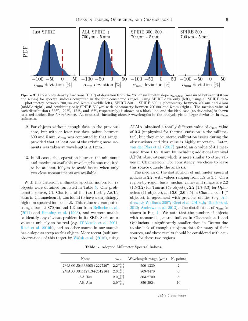
four considered cases. The results are shown in Fig. 3.

Deviations are largest when using SPIRE data only

(ranging from −93 % to 7 %, and with a median value

of −53 %), as expected since this is the shortest wave-

length range considered. For cases combining SPIRE

data with (sub)mm photometry from 700µm to 5 mm

(as used to estimate αtrue,mm), the most accurate values

are obtained excluding short SPIRE bands because the

considered fluxes become closer to the optically thin and

RJ regimes. In particular, combining SPIRE 500µm

photometry only with (sub)mm data yields a median

deviation of only 6 %, and in no case more than 25 %.

Table 4. Median Spectral Indices Computed at Different

Wavelength Ranges

Wavelength Range (µm) Spectral Index N. Objects

[µm]

65-105 0.1+0.9−0.7 87

95-165 0.4+0.7−0.7 66

155-255 1.0+0.7−0.7 82

245-355 1.2+0.5−0.7 80

345-505 1.3+0.6−0.4 74

495-890 1.9+0.9−0.7 58

860-1400 2.2+0.7−0.9 56

1200-5000 2.4+0.6−0.4 58

Note—Uncertainties are derived from 16th and 84th per-centiles.

Based on these results, we chose to estimate millimeter

slopes αmm in the following manner:

1. For objects with at least two data points between

800µm and 5 mm, those data were used to esti-

mate αmm.

Disks in Taurus, Ophiuchus, and Chamaeleon I 9

−100 −50 0 50αmm deviation [%]

PD

FJust SPIRE

−100 −50 0 50αmm deviation [%]

ALL SPIRE +700µm - 5 mm

−100 −50 0 50αmm deviation [%]

SPIRE 350, 500 +700µm - 5 mm

−100 −50 0 50αmm deviation [%]

SPIRE 500 +700µm - 5 mm

Figure 3. Probability density functions (PDF) of deviation from the “true” millimeter slope αmm,true (measured between 700µmand 5 mm) for spectral indices computed in the four considered ranges: using SPIRE data only (left), using all SPIRE data+ photometry between 700µm and 5 mm (middle left), SPIRE 350 + SPIRE 500 + photometry between 700µm and 5 mm(middle right), and combining only SPIRE 500µm with photometry between 700µm and 5 mm (right). The median value ofeach distribution (-53 %, -29 %, -17 %, and -6 %, respectively) is shown as a black line, and the ideal case (no deviation) is shownas a red dashed line for reference. As expected, including shorter wavelengths in the analysis yields larger deviation in αmm

estimates.

2. For objects without enough data in the previous

case, but with at least two data points between

500 and 5 mm, αmm was computed in that range,

provided that at least one of the existing measure-

ments was taken at wavelengths ≥ 1 mm.

3. In all cases, the separation between the minimum

and maximum available wavelengths was required

to be at least 100µm to avoid issues when only

two close measurements are available.

With this criterion, millimeter spectral indices for 78

objects were obtained, as listed in Table 5. One prob-

lematic source, CU Cha (one of the two Herbig Ae/Be

stars in Chamaeleon I), was found to have a surprisingly

high mm spectral index of 4.8. This value was computed

using fluxes at 870µm and 1.3 mm from Belloche et al.

(2011) and Henning et al. (1993), and we were unable

to identify any obvious problem in its SED. Such an α

value is unlikely to be real (e.g. D’Alessio et al. 2001;

Ricci et al. 2010b), and no other source in our sample

has a slope as steep as this object. More recent (sub)mm

observations of this target by Walsh et al. (2016), using

ALMA, obtained a totally different value of αmm value

of 0.3 (unphysical for thermal emission in the millime-

ter), but they encountered calibration issues during the

observations and this value is highly uncertain. Later,

van der Plas et al. (2017) quoted an α value of 3.1 mea-

sured from 1 to 10 mm by including additional archival

ATCA observations, which is more similar to other val-

ues in Chamaeleon. For consistency, we chose to leave

this source outside the analysis.

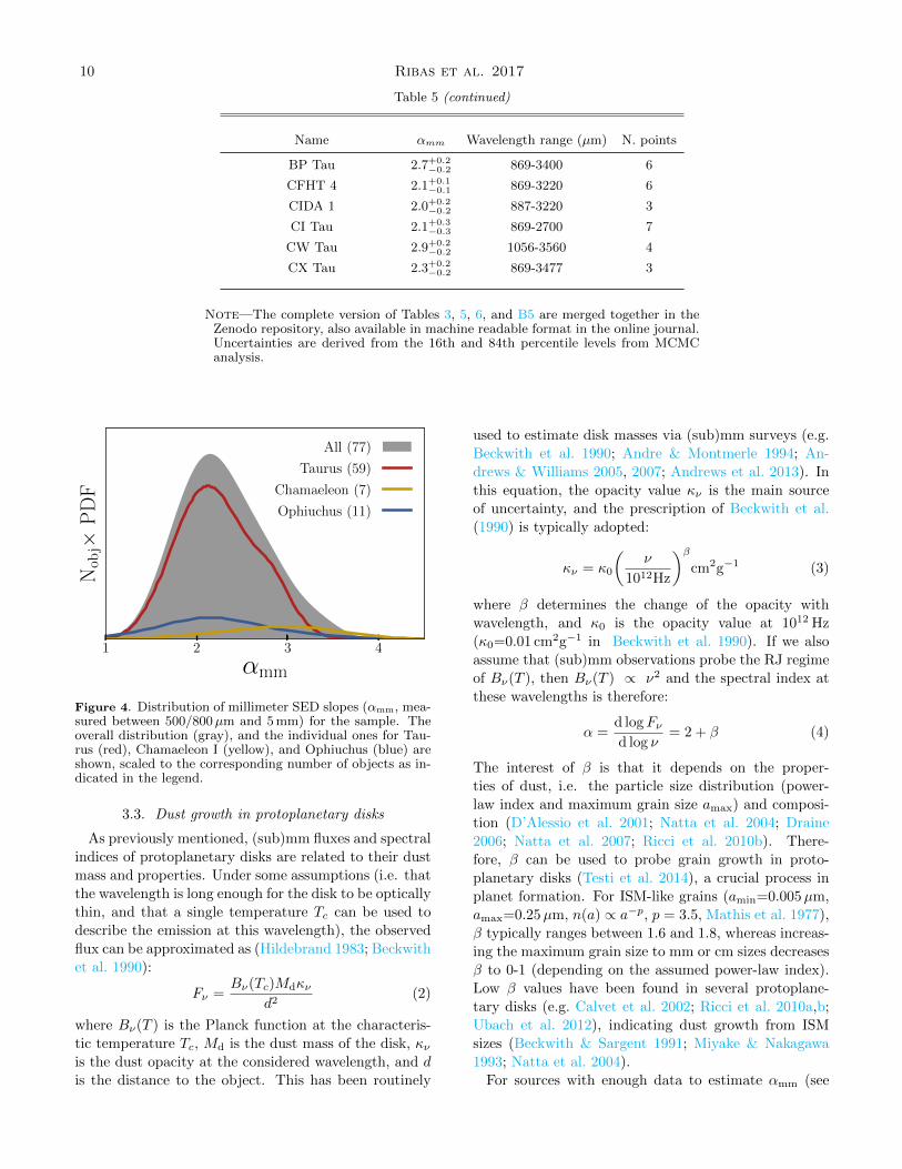
The median of the distribution of millimeter spectral

indices is 2.2, with values ranging from 1.5 to 3.5. On a

region-by-region basis, median values and ranges are 2.2

(1.5-3.2) for Taurus (59 objects), 2.2 (1.7-3.3) for Ophi-

uchus (11 objects), and 3.0 (2.0-3.5) in Chamaeleon I (7

objects), in agreement with previous studies (e.g. An-

drews & Williams 2007; Ricci et al. 2010a,b; Ubach et al.

2012; Andrews et al. 2013). The distribution of αmm is

shown in Fig. 4. We note that the number of objects

with measured spectral indices in Chamaeleon I and

Ophiuchus is significantly smaller than in Taurus due

to the lack of enough (sub)mm data for many of their

sources, and these results should be considered with cau-

tion for these two regions.

Table 5. Adopted Millimeter Spectral Indices.

Name αmm Wavelength range (µm) N. points

2MASS J04333905+2227207 2.2+0.3−0.3 500-1330 2

2MASS J04442713+2512164 2.0+0.1−0.1 869-3470 6

AA Tau 2.0+0.2−0.2 863-2700 8

AB Aur 2.9+0.1−0.1 850-2924 10

Table 5 continued

10 Ribas et al. 2017

Table 5 (continued)

Name αmm Wavelength range (µm) N. points

BP Tau 2.7+0.2−0.2 869-3400 6

CFHT 4 2.1+0.1−0.1 869-3220 6

CIDA 1 2.0+0.2−0.2 887-3220 3

CI Tau 2.1+0.3−0.3 869-2700 7

CW Tau 2.9+0.2−0.2 1056-3560 4

CX Tau 2.3+0.2−0.2 869-3477 3

Note—The complete version of Tables 3, 5, 6, and B5 are merged together in theZenodo repository, also available in machine readable format in the online journal.Uncertainties are derived from the 16th and 84th percentile levels from MCMCanalysis.

1 2 3 4

αmm

Nob

j×P

DF

All (77)

Taurus (59)

Chamaeleon (7)

Ophiuchus (11)

Figure 4. Distribution of millimeter SED slopes (αmm, mea-sured between 500/800µm and 5 mm) for the sample. Theoverall distribution (gray), and the individual ones for Tau-rus (red), Chamaeleon I (yellow), and Ophiuchus (blue) areshown, scaled to the corresponding number of objects as in-dicated in the legend.

3.3. Dust growth in protoplanetary disks

As previously mentioned, (sub)mm fluxes and spectral

indices of protoplanetary disks are related to their dust

mass and properties. Under some assumptions (i.e. that

the wavelength is long enough for the disk to be optically

thin, and that a single temperature Tc can be used to

describe the emission at this wavelength), the observed

flux can be approximated as (Hildebrand 1983; Beckwith

et al. 1990):

Fν =Bν(Tc)Mdκν

d2(2)

where Bν(T ) is the Planck function at the characteris-

tic temperature Tc, Md is the dust mass of the disk, κνis the dust opacity at the considered wavelength, and d

is the distance to the object. This has been routinely

used to estimate disk masses via (sub)mm surveys (e.g.

Beckwith et al. 1990; Andre & Montmerle 1994; An-

drews & Williams 2005, 2007; Andrews et al. 2013). In

this equation, the opacity value κν is the main source

of uncertainty, and the prescription of Beckwith et al.

(1990) is typically adopted:

κν = κ0

(ν

1012Hz

)βcm2g−1 (3)

where β determines the change of the opacity with

wavelength, and κ0 is the opacity value at 1012 Hz

(κ0=0.01 cm2g−1 in Beckwith et al. 1990). If we also

assume that (sub)mm observations probe the RJ regime

of Bν(T ), then Bν(T ) ∝ ν2 and the spectral index at

these wavelengths is therefore:

α =d logFνd log ν

= 2 + β (4)

The interest of β is that it depends on the proper-

ties of dust, i.e. the particle size distribution (power-

law index and maximum grain size amax) and composi-

tion (D’Alessio et al. 2001; Natta et al. 2004; Draine

2006; Natta et al. 2007; Ricci et al. 2010b). There-

fore, β can be used to probe grain growth in proto-

planetary disks (Testi et al. 2014), a crucial process in

planet formation. For ISM-like grains (amin=0.005µm,

amax=0.25µm, n(a) ∝ a−p, p = 3.5, Mathis et al. 1977),

β typically ranges between 1.6 and 1.8, whereas increas-

ing the maximum grain size to mm or cm sizes decreases

β to 0-1 (depending on the assumed power-law index).

Low β values have been found in several protoplane-

tary disks (e.g. Calvet et al. 2002; Ricci et al. 2010a,b;

Ubach et al. 2012), indicating dust growth from ISM

sizes (Beckwith & Sargent 1991; Miyake & Nakagawa

1993; Natta et al. 2004).

For sources with enough data to estimate αmm (see

Disks in Taurus, Ophiuchus, and Chamaeleon I 11

101 102 103

F1mm [mJy]

1.5

2.0

2.5

3.0

3.5

4.0α

mm

α = 3.7 (ISM)

αmm=2 (β=0)

Taurus

Chamaeleon

Ophiuchus

Figure 5. Predicted fluxes at 1 mm (scaled to 140 pc in thecase of Chamaeleon I) vs. spectral indices in the millime-ter for objects in Taurus (red), Chamaeleon I (yellow), andOphiuchus (blue). M2 and later-type stars are marked withblack crosses. Objects with a surrounding black border areclassified as (pre)transitional disks by their 13-31µm spectralindex. The α=2 line (corresponding to β=0 in the RayleighJeans regime and for optically thin disks) and the α value ofthe ISM (β = 1.7) are also shown.

Sec. 3.2), a line was fitted to their SEDs in log ν− logFνspace to predict the fluxes at 1 mm for each source.

Sources in Chamaeleon I were scaled to 140 pc to correct

to its different distance (160 pc) with respect to Taurus

and Ophiuchus. Figure 5 shows these 1 mm fluxes versus

the corresponding αmm values. Our results are very sim-

ilar to those found in previous studies (e.g. Ricci et al.

2010a,b; Testi et al. 2014). The lack of sources with low

F1mm and high αmm values is an observational bias: for

a given F1mm, higher αmm values result in more rapidlydeclining fluxes with increasing wavelength, and hence

more challenging detections (Ricci et al. 2010b).

An inspection of Figs. 4 and 5 shows that most objects

have αmm values between 2 and 3. Following Eq. 4,

this implies that most disks have β ≤ 1, pointing to

grain growth processes in them. Given the young ages

of sources in Ophiuchus and Taurus, this provides a

robust confirmation (with a larger sample and homo-

geneous treatment) of the fact that grain growth from

ISM-like to mm/cm sizes occurs quickly and early in the

disk lifetimes, as already found in previous studies (e.g.

Rodmann et al. 2006; Ricci et al. 2010b). The existence

of objects with αmm < 2 can not be explained with

the relation α = 2 + β because no physical dust model

produces negative β values (e.g. D’Alessio et al. 2001;

Draine 2006). For those cases, it is likely that the as-

sumption of the RJ regime does not hold: emission from

disks with a very cold mid-plane (e.g. Guilloteau et al.

2016) may depart from Fν ∝ ν2 significantly, yielding

flatter slopes. Late-type stars (considered here arbitrar-

ily as M2 or later type, as a compromise; see crosses

in Fig. 5) show αmm values below 2.5, with several

of them even below 2. Although this may hint at im-

portant dust growth around low-mass stars and brown

dwarfs, disks around these objects can be both colder

and smaller than their counterparts in more massive

stars, and therefore their emission could be optically

thick and/or outside the RJ regime. Resolved observa-

tions are needed to unambiguously determine the origin

of their low αmm values (see discussion in Ricci et al.

2014; Testi et al. 2016). Additionally, Chamaeleon I

shows an excess of high αmm - high F1mm fluxes with re-

spect to Taurus and Ophiuchus, which is discussed later

in the text (Sec. 4.3).

3.4. Millimeter indices and other tracers of disk

evolution

Using the compiled data, we also searched for correla-

tions of the mm slopes measured in Sec. 3.2 with other

indicators of disk evolution; namely, the strength and

shape of the 10µm silicate feature probing dust growth

in the upper layers of disks, and tracers of cavities in

them. The presence of gaps and cavities in the dust spa-

tial distribution in disks was first inferred in their SEDs

due to a deficit of near/mid-IR excess in some objects

(Strom et al. 1989), and was later confirmed via direct

imaging (e.g. Andrews et al. 2011). These particular

disks with a hole are called transitional disks (or pre-

transitional disks, if they have ring-like gaps separating

their inner and outer regions), and they have gained

significant attention in the last two decades due to the

exciting possibility of these gaps/holes being produced

by forming giant planets (see Espaillat et al. 2014, for a

recent review). Because they lack material in their inner

regions, their near/mid-IR emission is reduced and they

have steeper SEDs at these wavelengths with respect

to full disks, a fact that has been used in the past to

identify transitional disk candidates (e.g. Forrest et al.

2004; Brown et al. 2007; Merın et al. 2010; McClure

et al. 2010). The presence of giant planets directly im-

plies that grains must have suffered significant growth,

and hence it is possible that dust in transitional disks

may have different properties. In the case of full disks,

dust settling toward the disk mid-plane also decreases

the IR emission, producing a change in their slopes at

these wavelengths (e.g. Furlan et al. 2005).

12 Ribas et al. 2017

Table 6. IR spectral indices and 10µm silicate feature properties.

Name α5.3−12.9 α12.9−31 Silstrength Silshape

2MASS J04141188+2811535 -0.6+0.1−0.1 -0.57+0.08

−0.08 0.6+0.2−0.3 0.94+0.07

−0.07

2MASS J04153916+2818586 0.47+0.09−0.08 -1.43+0.07

−0.07 0.11+0.08−0.1 0.96+0.08

−0.07

2MASS J04155799+2746175 0.02+0.08−0.08 0.1+0.2

−0.1 0.4+0.07−0.11 0.99+0.06

−0.05

2MASS J04163911+2858491 0.5+0.2−0.2 0.0+0.2

−0.2 0.1+0.2−0.1 1.0+0.1

−0.1

2MASS J04201611+2821325 -0.01+0.08−0.08 0.0+0.4

−0.3 0.05+0.09−0.05 0.92+0.05

−0.05

2MASS J04202144+2813491 0.0+0.3−0.2 -1.2+0.3

−0.3 -0.3+0.2−0.2 2.1+1.7

−0.6

2MASS J04202606+2804089 -1.2+0.1−0.1 -1.39+0.06

−0.06 1.4+0.2−0.2 0.92+0.05

−0.05

2MASS J04210795+2702204 -0.1+0.7−26.7

2MASS J04214631+2659296 -0.0+0.4−0.4 -0.2+3.2

−0.7 0.2+0.7−0.3 0.9+0.3

−0.3

2MASS J04230607+2801194 0.15+0.08−0.07 -0.9+0.1

−0.1 0.24+0.14−0.07 0.92+0.06

−0.05

Note—The complete version of Tables 3, 5, 6, and B5 are merged together in theZenodo repository, also available in machine readable format in the online journal.Uncertainties derived from 16th and 84th percentile levels from 1000 bootstrappingiterations.

Dust growth is thought to occur mostly in the disk

mid-plane, where the density is higher and tempera-

tures lower than in the upper layers (see the review in

Testi et al. 2014), where the 10µm silicate feature orig-

inates. Therefore, a relation between this feature and

αmm would imply a co-evolution of grains in the up-

per layers of disks and their mid-plane. Lommen et al.

(2007, 2010) found a tentative correlation between sili-

cate strengths and shapes (a tracer of grain crystallinity)

for YSOs in different star-forming regions, but Ricci

et al. (2010a) did not find any in Ophiuchus. A later

study by Ubach et al. (2012) revealed only a weak, also

tentative correlation between the strength of this featureand the αmm for some sources in Taurus, Ophiuchus,

Chamaeleon, and Lupus. We used the compiled IRS

spectra (when possible) to compute silicate strengths

and shapes following Furlan et al. (2006) and Kessler-

Silacci et al. (2006) respectively. The resulting values are

listed in Table 6, and the process is described in more

detail in Appendix C. Spearman rank tests revealed no

significant correlations between the strength/shape of

the silicate feature and αmm, neither for any or these

regions individually nor for the whole sample.

Near/mid-IR spectral indices αIR were also computed,

following McClure et al. (2010), using the IRS spec-

tra between 5.3 and 12.9µm (taken as the median flux

within a range of ±0.2µm centered around each of these

wavelengths), and the slope between 12.9 and 31µm.

Spearman rank tests between αIR and αmm showed these

two quantities to be uncorrelated, both for the whole

sample and for each individual region. We also iden-

tified (pre)transitional disks by selecting objects with

spectral indices between 13 and 31µm < -1.4 (in Fνspace, as computed from their IRS spectra), following

the criterion in McClure et al. (2010). These sources

are encircled in Fig. 5 for comparison, but no obvious

trend was found for them. These results suggest that the

dust population in the midplane/outer regions of transi-

tional disks (at least those which gaps have a detectable

effect in the IR slope of their SEDs) is not substantially

different than those of their full counterparts.

4. A SIMPLE DISK MODEL

After the analysis of spectral indices in Sec. 3, we ap-

plied the simple disk model in Beckwith et al. (1990)

to the compiled long-wavelength (≥ 70µm) data. This

model does not depict a physically self-consistent disk,

but instead assumes that the emission arises from a ver-

tically isothermal one. The SED of such a disk can be

written as:

Fν =cos i

d2

∫ Rd

rin

Bν(T (r))(1− e−τν(r) sec i)2πr dr (5)

where i is the inclination, d is the distance to the source,

rin and Rd are the inner and outer radii of the disk,

Bν(T (r)) is the Planck function at the temperature

T (r), and τν(r) is the optical depth at the given fre-

quency ν and radius r. This optical depth is the product

of the opacity at the corresponding frequency (κν) and

the radial surface density profile (Σ(r)). We assume the

radial dependence of the temperature and surface den-

Disks in Taurus, Ophiuchus, and Chamaeleon I 13

sity to follow a power law:

T (r) = T0

(r

r0

)−q(6)

Σ(r) = Σ0

(r

r0

)−p(7)

where T0 and Σ0 are the temperature and surface den-

sity at an arbitrary radius r0. The opacity law is also

assumed to be a power law following Beckwith & Sar-

gent (1991), as shown in Eq. 3. Therefore, the optical

depth at a given wavelength (frequency) and radius can

be written as:

τν(r) = Σ0κ0

(r

r0

)−p(ν

230 GHz

)β(8)

Here, κ0 is the opacity value at 230 GHz (we consider

230 GHz instead of 1000 GHz as in Eq. 3, due to the

common use of 1.3 mm as the reference wavelength).

However, κ0 also depends on the maximum grain size

(e.g. D’Alessio et al. 2001), and it should not be left

constant when modeling while changing β (this could

introduce artificial trends in the modeling results, e.g.

Ricci et al. 2010b). We therefore combined Σ0 and κ0

into τν,r0 , i.e. the optical depth at the arbitrary radius

r0 (set to 10 au in our study) and at 230 GHz:

τν(r) = τ1.3mm,10 au

(r

10 AU

)−p(ν

230 GHz

)β(9)

With this setup, there are a total number of eight free

parameters in this model: τ1.3mm,10 au, rin, Rd, T10au, p,

q, i, and β. Because we will model far-IR and (sub)mm

fluxes, the inner radius does not have a crucial effect in

our modeling and was fixed to 0.01 au following Andrews

& Williams (2005) - a rough estimate of where dust sub-

limation occurs (Dullemond et al. 2001; Muzerolle et al.

2003). Therefore, seven free parameters remain.

Spectral indices α ∼ 2 can be produced both by com-

pact, optically thick disks (small Rd, typically < 50 au,

high τ1.3mm,10 au, and unconstrained β), or bigger, op-

tically thin disks with large dust grains (larger and un-

constrained Rd, low τ1.3mm,10 au and β values). As a

result, τ1.3mm,10 au, Rd, and β estimates become degen-

erate in these cases from SED fitting alone. Observation-

ally, most resolved disks have been found to extend for

about (or more than) 50-150 au (Andrews et al. 2010;

Ricci et al. 2010a,b, 2014), but the difficulty in resolv-

ing smaller and usually fainter disks introduces an im-

portant bias. Recent high-resolution observations have

identified a population of small disks (e.g. Pietu et al.

2014; Osorio et al. 2016; Testi et al. 2016), and conse-

quently they cannot be ruled out in the analysis. In an

effort to break this degeneracy, we gathered disk radii

from Andrews & Williams (2007) ,Ricci et al. (2010a,b),

Pietu et al. (2014), and Pascucci et al. (2016). In the last

case, disk radii were estimated from FWHM measure-

ments converted to physical sizes using the distance to

Chamaeleon I, and uncertainties of 25 % were assigned.

For each source, we aim at fitting data between 70µm

and 5 mm. We also included the processed SPIRE spec-

tra (when available) after binning them in five points

to avoid giving them excessive weight, by simply di-

viding the corresponding wavelength range in five equal

sub-ranges, and adopting the median flux value in each

of them. For consistency with our previous Herschel

data processing, we assigned 20 % uncertainties to these

data. Inspection of uncertainties of the ancillary data

revealed that many of them were underestimated, prob-

ably due to a lack of the systematic contribution. We

circumvented the issue by assigning 20 % uncertainties

to measurements with smaller values. We note that the

effect of this is to produce more conservative uncertain-

ties in our final estimates, and it should not affect our

results. We adopted a Bayesian methodology and used

the ensemble samplers with affine invariance (Good-

man & Weare 2010) variation of the Markov Chain

Monte Carlo (MCMC) method via the emcee software

(Foreman-Mackey et al. 2013). Priors were chosen based

on the interest of each parameter and typical values in

previous studies:

1. Rd: if the source had information about its ra-

dius from Andrews & Williams (2007), Ricci et al.

(2010a), or Ricci et al. (2010b) where a range of

values was quoted, a flat prior was assumed over

the corresponding ranges. For resolved objects in

Pietu et al. (2014) or Pascucci et al. (2016), a

Gaussian prior was used centered at the reported

disk radii, with a standard deviation equal to thecorresponding uncertainty. For objects with no re-

solved information, a flat prior from 10 to 300 au

was assumed.

2. τ1.3mm,10AU : flat prior from 10−3 to 103, consider-

ing extreme values of κ1.3mm and Σ10 au. Because

the range extends for several orders of magnitude,

this parameter was explored in logarithmic scale.

3. T10AU : flat prior from 5 to 500 K.

4. p: flat prior from 0.5 to 1.5. This covers fiducial

values used in modeling (e.g. Andrews & Williams

2005).

5. q: Gaussian prior centered at 0.5 with a standard

deviation of 0.1. This accounts for the typical

spread obtained in models (e.g. Chiang & Goldre-

ich 1997; D’Alessio et al. 1998).

14 Ribas et al. 2017

6. i: inclination values larger than 80 degrees were

excluded to avoid issues at very high inclinations.

For the remaining inclinations, a geometric prior

sin(i) was used.

7. β: flat prior from 0 to 2.5, based on β measure-

ments of disks (Ricci et al. 2010a,b; Ubach et al.

2012).

As already mentioned, the considered models have

seven free parameters. In the adopted approach, the

use of restrictive priors for some of them (e.g. p, q, in-

clination) provides additional information to the fitting

process. We chose to model objects with data avail-

able for at least seven different wavelengths, combining

photometry and the binned SPIRE spectra. We also re-

quired the minimum wavelength available to be smaller

than 200µm and the maximum one to be above 800µm

to guarantee a reasonable coverage of the far-IR/mm

part of the SEDs. Sixty-three objects in the sample

meet this criterion: 40 in Taurus, 5 in Ophiuchus, and

14 in Chamaeleon I. From these, 28 had some informa-

tion about their disk radii from resolved high-resolution

observations. In the emcee setup for each source, 40,000

iterations with 50 walkers were run, and the last 10,000

steps were used to generate our posterior distributions.

The chains were visually inspected for convergence, and

we also checked that the adopted burn-in range (the dis-

carded initial 30,000 steps) was at least five times the

corresponding autocorrelation time.

The adopted procedure yielded satisfactory fits in all

cases, and the obtained posterior functions revealed that

τ1.3mm,10 au, T10au, and β are generally constrained to

some extent. As expected, the posteriors of p, q, and

i follow the assumed priors because they are largely

unconstrained with SEDs alone. Despite our efforts to

include resolved information, some objects displayed a

bi-modal behavior in their Rd, τ1.3mm,10 au, and β pos-

teriors, as corresponds to the degenerate case formerly

mentioned. Although the distributions for T10au are

still informative (the Bayesian methodology naturally

accounts for the existence of degeneracies), the bi-modal

posteriors of τ1.3mm,10 au makes them complex to ana-

lyze, and we excluded these objects when focusing on

these parameters in particular. The obtained results for

τ1.3mm,10 au, T10au, and β are reported in Table 7. An

example of a well-behaved source (DL Tau) is shown in

Fig. 6.

Table 7. Modeling Results (Median, 16th, and 84th percentiles).

Name τ1.3mm,10AU β T10AU [K]

AA Tau† −0.6+0.5−0.3 0.9+0.3

−0.3 43+6−8

AB Aur −1.1+0.3−0.2 1.4+0.1

−0.2 178+35−51

BP Tau −0.3+0.3−0.3 1.4+0.3

−0.4 31+5−7

CIDA 7 −0.8+0.5−2.6∗ 0.7+0.5

−0.9∗ 34+6−7

CIDA 9 −0.3+0.6−2.0∗ 0.9+0.6

−0.9∗ 35+5−6

CI Tau† −0.2+0.3−0.2 1.3+0.3

−0.4 47+6−10

CW Tau† −0.0+0.2−0.2 1.9+0.6

−0.4 58+6−5

CY Tau† 0.1+0.4−0.3 0.7+0.4

−0.4 25+3−5

DD Tau −1.4+0.6−1.9 0.3+0.2

−0.6 66+16−49

DE Tau† 0.5+0.4−1.6∗ 1.5+0.9

−0.7∗ 53+8−7

DG Tau 0.1+0.4−0.4 0.7+0.2

−0.4 94+13−20

DH Tau 0.4+1.5−1.7∗ 0.5+0.4

−1.1∗ 37+6−8

DK Tau 0.6+1.9−1.7∗ 0.5+0.3

−1.1∗ 50+9−20

DL Tau† 0.0+0.3−0.3 1.0+0.2

−0.2 42+4−8

DN Tau† −0.3+0.3−0.3 0.6+0.3

−0.4 36+5−7

DO Tau† −0.6+0.3−0.3 0.3+0.1

−0.1 78+11−14

DQ Tau 0.1+0.4−0.3∗ 1.8+0.7

−0.4∗ 38+7−10

DS Tau −0.7+0.5−1.4∗ 0.6+0.4

−0.7∗ 29+5−6

FM Tau† 1.5+1.1−1.0∗ 1.1+0.8

−0.9∗ 34+6−6

FN Tau −1.5+0.6−2.0 0.2+0.1

−0.5 85+25−66

FT Tau† −0.4+0.8−1.9 0.5+0.3

−0.6 43+6−11

FV Tau −1.6+0.5−0.3∗ 1.0+0.5

−0.6∗ 57+13−42

GM Aur† −0.3+0.4−0.3 1.5+0.2

−0.2 54+6−10

GO Tau† −0.3+0.3−0.2 1.5+0.2

−0.3 30+3−5

Haro 6-13 −0.5+0.4−0.3 0.6+0.2

−0.2 78+11−15

HK Tau −0.9+0.3−0.3 0.9+0.2

−0.2 55+7−10

IRAS 04125+2902 −1.1+0.4−0.4 1.0+0.4

−0.5 47+8−10

IRAS 04385+2550 −1.0+0.5−0.3 0.6+0.1

−0.2 66+10−16

IP Tau −0.9+0.6−0.2∗ 1.7+1.2

−0.5∗ 24+5−16∗

IQ Tau† −0.4+0.3−0.3 0.8+0.3

−0.3 37+5−7

LkCa 15 −0.0+0.3−0.3 1.4+0.2

−0.3 42+4−8

RW Aur −1.2+0.7−3.1∗ 0.1+0.1

−1.4∗ 91+23−80

RY Tau −0.3+0.5−0.5 0.6+0.2

−0.6 92+13−19

UX Tau A+C −0.7+0.4−0.3 0.8+0.3

−0.4 59+8−12

UY Aur −1.3+0.4−0.3 0.9+0.2

−0.2 78+13−18

UZ Tau A† −0.3+0.4−0.3 0.7+0.3

−0.3 48+6−10

V710 Tau −0.4+0.3−0.2∗ 1.7+0.5

−0.6∗ 30+3−5

V807 Tau −1.6+0.5−0.5 0.6+0.4

−0.5 51+13−32

V836 Tau† −0.2+0.3−0.7 0.5+0.3

−1.1 34+6−5

V892 Tau −0.6+0.4−0.3 0.6+0.1

−0.2 153+28−44

ZZ Tau IRS −0.3+0.3−0.2 2.2+0.4

−0.2 54+7−12

DOAR16AB −1.1+0.5−1.7∗ 0.6+0.4

−0.8∗ 53+10−23

Table 7 continued

Disks in Taurus, Ophiuchus, and Chamaeleon I 15

−0.8

−0.4

0.0

0.4

log

10(τ

1.3mm,1

0AU)

32

40

48

56

64

T10A

U[K

]

0.5

1.0

1.5

2.0

β

0.6

0.8

1.0

1.2

1.4

p

0.3

0.4

0.5

0.6

0.7

q

160

180

200

220

240

Rd [AU]

20

40

60

80

incl

[deg

]

−0.8

−0.4

0.0

0.4

log10(τ1.3mm,10AU)

32 40 48 56 64

T10AU [K]

0.5

1.0

1.5

2.0

β

0.6

0.8

1.0

1.2

1.4

p

0.3

0.4

0.5

0.6

0.7

q

20 40 60 80

incl [deg]

100 1000

λ [µm]

10−2

10−1

100

Fν

[Jy]

DL Tau

Figure 6. Fitting results for DL Tau. The corner plot shows the posterior distributions for parameters and the corresponding2D projections. Vertical dashed lines show the 16th, 50th, and 84th percentiles. The inset shows the fitted photometry (redcircles) and SPIRE spectrum (yellow line), together with 1000 models randomly selected from the posterior distributions (darkarea). This object is a well-behaved case for which τ1.3mm,10AU , T10AU , and β do not become degenerate.

16 Ribas et al. 2017

Table 7 (continued)

Name τ1.3mm,10AU β T10AU [K]

DOAR25† −0.1+0.3−0.3 0.6+0.2

−0.2 49+5−7

GSS39 0.4+0.4−0.4 0.9+0.3

−0.4 39+5−8

SR21AB† −1.3+0.4−0.3 1.4+0.1

−0.2 106+14−22

IRS48 −1.4+0.4−0.3 0.7+0.2

−0.3 236+73−133

IRS49 −0.9+0.8−2.8∗ 0.3+0.2

−1.1∗ 65+13−41

WSB60† −0.6+0.6−0.4 0.6+0.3

−0.3 44+7−8

ROX-44† −1.1+0.4−0.4 0.1+0.1

−0.2 97+25−41

SX Cha −1.2+0.5−0.8 0.4+0.3

−0.5 50+12−29

SZ Cha −0.2+0.3−0.2 1.8+0.3

−0.4 62+8−13

TW Cha† −0.2+0.4−1.9∗ 0.5+0.4

−1.1∗ 35+6−5

CR Cha† 0.1+0.2−0.2 2.2+0.3

−0.2 52+6−7

CS Cha† 0.1+0.4−0.3∗ 1.6+0.9

−0.7∗ 67+11−9

CT Cha −0.0+0.6−2.1∗ 0.7+0.5

−1.1∗ 41+6−7

CU Cha −0.2+0.3−0.3 2.3+0.3

−0.2 156+29−39

T33A† −0.5+0.3−0.4∗ 1.1+0.3

−1.1∗ 83+15−19

VZ Cha 0.2+0.6−1.7∗ 1.1+0.8

−0.9∗ 31+4−7

B43 0.9+1.0−1.4∗ 1.0+0.7

−1.0∗ 26+3−4

T42† −1.3+0.2−0.2 2.1+0.3

−0.3 88+11−18

WW Cha† 0.2+0.3−0.2 1.8+0.5

−0.5 99+12−15

T47† −0.6+0.3−1.5 0.3+0.2

−0.8 41+7−7

CV Cha† 0.3+1.0−1.9∗ 1.0+0.7

−1.0∗ 80+15−15

T56† −0.7+0.3−1.4∗ 0.6+0.4

−1.1∗ 46+8−7

Notes.† Object with Rd constraints from resolved observations.∗ Unconstrained/bimodal distribution.

Before analyzing these results, it is important to men-

tion that the disk model used here is a very simplis-

tic approximation. It assumes a fixed inner radius

and an axisymmetric geometry. More importantly, it

does not include a vertical temperature gradient or dust

mixing/settling, which produce flared disks required to

properly explain far-IR fluxes of disks (e.g. Kenyon &

Hartmann 1987; Calvet et al. 1992). We have also as-

sumed a power-law opacity law longward of ∼ 70µm,

which is not realistic in the presence of different dust

species (e.g. D’Alessio et al. 2001; Draine 2006). These

two last issues combined are especially relevant for β

estimates, which may therefore be higher than the ex-

pected α = 2 + β relation. Thus, although they can

provide interesting insights and comparisons, the results

from the modeling should therefore be considered with

caution.

4.1. Optical depth and β values

Despite having included disk size estimates from the

literature, some objects lacked that information, or the

measured size ranges were not restrictive enough to

avoid the degeneracy in the fitting process. Here, we

limit our analysis to non-degenerate τ1.3mm,10 au and β

distributions, as revealed by their well-behaved distri-

butions (i.e. constrained and not bi-modal). Therefore,

40 objects were used to study these parameters, 28 in

Taurus, 6 in Ophiuchus, and 6 in Chamaeleon I.

The ensemble distributions of τ1.3mm,10 au, and β for

each region (produced by randomly selecting 1 million

positions from the individual posteriors) are shown in

the top and middle panels in Fig. 73. We first note that

the low number of sources remaining after the adopted

curation processes both in Ophiuchus and Chamaeleon I

is an obvious caveat to our interpretation, and therefore

it cannot be extrapolated to the whole sample. However,

they can still be used to investigate possible differences

among regions, under the assumption that these distri-

butions are not very different from the underlying ones

(or at least that they are different in similar ways). In

the following, we assume this to be the case, bearing

in mind that additional observations may improve and

modify some of these results.

The distribution of optical depth values at 10 au and

1.3mm (Fig. 7, top) has its maximum at log τ1.3mm,10 au

= -0.25 (corresponding to τ1.3mm,10 au ∼ 0.5), and a sec-

ondary peak at log τ1.3mm,10 au = −1. We note that the

shape of this distribution is determined mostly by Tau-

rus, given the lack of sufficient long-wavelength data for

most objects in Chamaeleon I and Ophiuchus, and the

distributions in these regions appear to be broader than

the one in Taurus (again, this interpretation is limited by

the small number statistics in these regions). For com-

parison, reasonable assumptions about the dust opacity

and surface density based on observations of the solar

system bodies yield τ1 mm=1 at ∼ 10 au for the Minimum

Mass Solar Nebula (Davis 2005), suggesting that several

of the modeled protoplanetary disks may have optical

depth profiles (and hence possibly surface densities) sim-

ilar to that of the parental disk of the solar system. In

the case of β, values smaller than the one measured for

the ISM (∼1.6-2; see e.g. Draine 2006, and references

therein) imply some degree of grain growth. Almost

the entirety of the Taurus and Ophiuchus distributions

(and part of Chamaeleon I) are constrained within that

value, in correspondence with the observational result

3 Given the large number of MCMC steps and the computa-tional requirement to compute KDEs in these particular cases, wedisplayed these distributions using histograms with a large (100)number of bins.

Disks in Taurus, Ophiuchus, and Chamaeleon I 17

2 1 0 1 2log10(τ1.3mm, 10AU)

Ens

embl

e di

stri

butio

n All (40)Taurus (28)

Ophiuchus (6)Chamaeleon (6)

0.0 0.5 1.0 1.5 2.0 2.5β

Ens

embl

e di

stri

butio

n All (40)Taurus (28)

Ophiuchus (6)Chamaeleon (6)

25 50 75 100 125 150T10AU

Ens

embl

e di

stri

butio

n All (61)Taurus (39)

Ophiuchus (8)Chamaeleon (14)

Figure 7. Ensemble distributions for τ1.3mm,10 au (top), β(middle), and T10AU (bottom) for each region, normalizedto the number of objects in each association. Sources withbi-modal (degenerate) and flat (uninformative) distributionshave been excluded. The number of objects in each case isindicated in the legend.

discussed in Sec. 3.3. As with αmm, Chamaeleon I shows

a different behavior (an excess of high β values) that will

be discussed further on. We note that the distributions

of β should be considered with caution, not only due to

the aforementioned caveats, but also because degener-

ate cases have been removed from the analysis. Because

these occur when α = 2, this procedure inevitably dis-

cards objects with β ∼ 0. There is a tentative bimodal-

ity in both distributions, and especially in the case of

β, with a tentative secondary peak occurring at ∼ 1.4-

1.5. Given the limited size of the modeled sample and

the simplicity of the models used, we do not investigate

this issue in detail here. However, we speculate that, if

real, it may hint at a quick transition from micron-sized

grains (large β values) to mm/cm-sized dust (smaller β).

We also inspected our results in the τ1.3mm,10 au ver-

sus β space. Individually, these two parameters affectthe optical depth—and are therefore correlated—but a

more general correlation may also exist as a result of

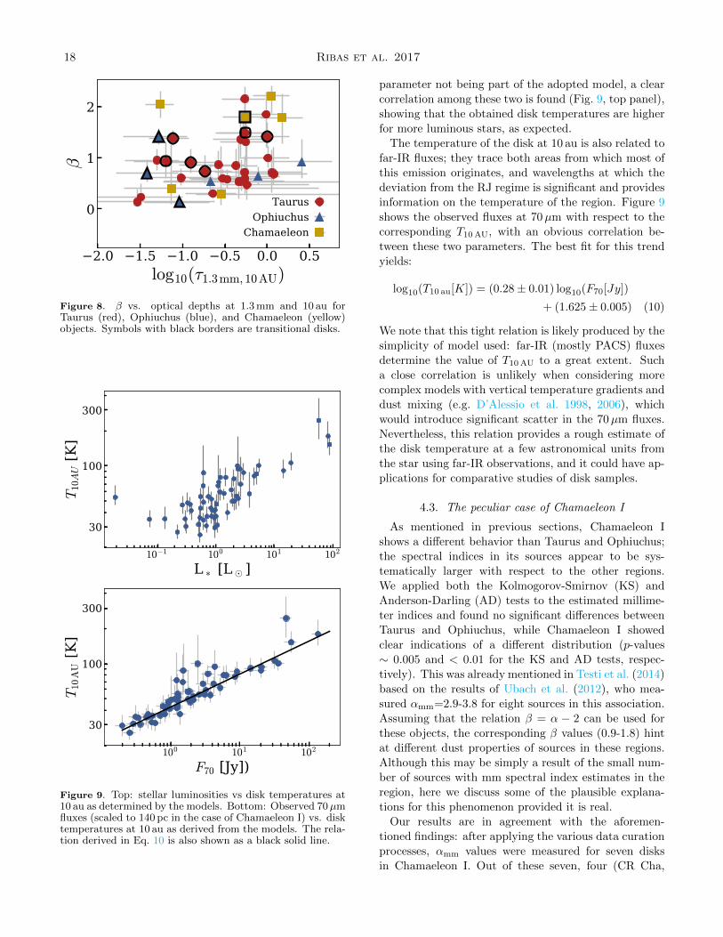
disk evolution. Fig. 8 shows that objects with low β

values (. 1) spread through optical depth values from

log10(τ1.3mm,10 au) = −1.5 to 0.5. However, a lack of

low optical depths is found for βs above that threshold,

an expected effect from an observational bias toward

bright sources: mm fluxes decrease faster with increas-

ing wavelengths for steeper β values, and only massive

disks (likely to be optically thicker) are detectable. Al-

though such an effect could also be partially produced

by disk evolution (disk masses decrease with time, and

dust growth leads to smaller βs), more complex mod-

els are required to quantify how much (if any) of this

paucity of low β - low optical depth values is due to disk

evolution itself. Like Fig. 5, Fig. 8 also shows the posi-

tion of (pre)transitional disks (as classified in Sec. 3.4),

with no obvious difference between these sources and

full disks.

4.2. Disk temperatures at 10 au

The modeling process also yielded estimates of the

disk temperature at 10 au. For this parameter—

even when the disk radii, optical depth, and β are

degenerate— the posterior T10 au is constrained to some

extent, in most cases. Only two of the modeled sources

displayed an uninformative (∼ flat) posterior distribu-

tion and were excluded from the analysis, leaving 39 ob-

jects in Taurus, 8 in Ophiuchus, and 14 in Chamaeleon I.

Fig. 7 (bottom) shows the results for the three regions,

all of them showing a distribution that peaks at ∼40-

50 K with a lower probability tail extending to ∼ 100-

150 K due to the effect of high inclinations (see corner

plot in Fig. 6).

The obtained T10 au values can be used to test the

general performance of these models by comparing them

with the luminosity of their host star: despite the former

18 Ribas et al. 2017

2.0 1.5 1.0 0.5 0.0 0.5log10(τ1.3mm, 10AU)

0

1

2

β

TaurusOphiuchus

Chamaeleon

Figure 8. β vs. optical depths at 1.3 mm and 10 au forTaurus (red), Ophiuchus (blue), and Chamaeleon (yellow)objects. Symbols with black borders are transitional disks.

10−1 100 101 102

L ∗ [L ¯ ]

30

100

300

T10AU [K

]

100 101 102

F70 [Jy])

30

100

300

T10

AU [K

]

Figure 9. Top: stellar luminosities vs disk temperatures at10 au as determined by the models. Bottom: Observed 70µmfluxes (scaled to 140 pc in the case of Chamaeleon I) vs. disktemperatures at 10 au as derived from the models. The rela-tion derived in Eq. 10 is also shown as a black solid line.

parameter not being part of the adopted model, a clear

correlation among these two is found (Fig. 9, top panel),

showing that the obtained disk temperatures are higher

for more luminous stars, as expected.

The temperature of the disk at 10 au is also related to

far-IR fluxes; they trace both areas from which most of

this emission originates, and wavelengths at which the

deviation from the RJ regime is significant and provides

information on the temperature of the region. Figure 9

shows the observed fluxes at 70µm with respect to the

corresponding T10 AU, with an obvious correlation be-

tween these two parameters. The best fit for this trend

yields:

log10(T10 au[K]) = (0.28± 0.01) log10(F70[Jy])

+ (1.625± 0.005) (10)

We note that this tight relation is likely produced by the

simplicity of model used: far-IR (mostly PACS) fluxes

determine the value of T10 AU to a great extent. Such

a close correlation is unlikely when considering more

complex models with vertical temperature gradients and

dust mixing (e.g. D’Alessio et al. 1998, 2006), which

would introduce significant scatter in the 70µm fluxes.

Nevertheless, this relation provides a rough estimate of

the disk temperature at a few astronomical units from

the star using far-IR observations, and it could have ap-

plications for comparative studies of disk samples.

4.3. The peculiar case of Chamaeleon I

As mentioned in previous sections, Chamaeleon I

shows a different behavior than Taurus and Ophiuchus;

the spectral indices in its sources appear to be sys-

tematically larger with respect to the other regions.

We applied both the Kolmogorov-Smirnov (KS) and

Anderson-Darling (AD) tests to the estimated millime-

ter indices and found no significant differences between

Taurus and Ophiuchus, while Chamaeleon I showed

clear indications of a different distribution (p-values

∼ 0.005 and < 0.01 for the KS and AD tests, respec-

tively). This was already mentioned in Testi et al. (2014)

based on the results of Ubach et al. (2012), who mea-

sured αmm=2.9-3.8 for eight sources in this association.

Assuming that the relation β = α − 2 can be used for

these objects, the corresponding β values (0.9-1.8) hint

at different dust properties of sources in these regions.

Although this may be simply a result of the small num-

ber of sources with mm spectral index estimates in the

region, here we discuss some of the plausible explana-

tions for this phenomenon provided it is real.

Our results are in agreement with the aforemen-

tioned findings: after applying the various data curation

processes, αmm values were measured for seven disksin Chamaeleon I. Out of these seven, four (CR Cha,

Disks in Taurus, Ophiuchus, and Chamaeleon I 19

SZ Cha, WW Cha, and T33 A) have values larger than

α > 3 (and the number would go up to five if we were

to include the α value for CU Cha in van der Plas et al.

2017). This represents 55-60 % of the sample with avail-

able spectral index estimates in this region. For compar-

ison, the fractions of objects with α > 3 in Taurus and

Ophiuchus are 2 % (1/58) and 9 % (1/11), respectively.

A similar (but more uncertain) result is found when

analyzing the β distributions from the models, where

Chamaeleon I shows an excess of high values (> 1.5).

Although an in-depth analysis of each data set would

be required to completely rule out systematic problems

in any of the sources of ancillary (sub)mm data used

for Chamaeleon I, our inspection of the corresponding

SEDs revealed no apparent issue—and this result is still

present when using individual studies to estimate spec-

tral indices. We therefore discard the possibility of this

being a data-processing problem.

Chamaeleon I is estimated to be the oldest region of

the considered sample, and hence its steeper (sub)mm

slopes could be the result of dust evolution in its disks.

These mm spectral indices imply high β values, sug-

gestive of a decrease in the maximum grain size in the

outer regions of these disks. Such a trend is expected

from the inward drift of mm/cm-sized grains in the pres-

ence of gas: at these sizes, dust particles start experi-

encing a head wind from the gas, losing angular momen-

tum and spiraling inward (Adachi et al. 1976; Weiden-

schilling 1977; Takeuchi & Lin 2002). This mechanism

clears out the outer regions of the disk of mm/cm-sized

grains (if they are not replenished by other means) and

effectively decreases the value of amax, thus increasing β

as a function of radius (e.g. Birnstiel et al. 2010; Pinilla

et al. 2012). Disk lifetimes are on the order of 5-10 Myr

(Haisch et al. 2001; Hernandez et al. 2007; Ribas et al.

2015), but the inward migration of mm/cm grains is esti-

mated to be much faster (104-105 years, e.g. Takeuchi &

Lin 2005; Brauer et al. 2007); braking mechanisms, such

as dust accumulation at pressure bumps, are required to

slow down this inward migration (e.g. Zhu et al. 2011;

Pinilla et al. 2012) and explain observed mm spectral in-

dices in disks (Testi et al. 2014). A possible explanation

for the higher αmm values in Chamaeleon I is that dust

migration has significantly altered disks in this region,

but is still not as important in Taurus and Ophiuchus.

However, Chamaeleon I sources with steep β values are

also among the brightest objects at mm wavelengths in

the sample (Fig. 5), in contradiction with the expected

decline of disk masses with time (produced by viscous

evolution and/or the decrease in mm opacities caused

by inward migration of dust). If the fact that disks in

Chamaeleon I are older was the only reason for differ-

ences in spectral indices, then these disks would have

needed to be initially more massive than their counter-

3000400050006000Teff [K]

10−2

10−1

100

101

102

L∗

[L¯]

TaurusChamaeleonOphiuchus

1 Myr2 Myr3 Myr5 Myr

SZ ChaCR Cha

T33A

WW Cha

Figure 10. H-R diagram for sources with αmm > 2.5 and T∗between 3000 and 7000 K. Objects in Taurus (red circles),Chamaeleon I (yellow squares), and Ophiuchus (blue trian-gles) are shown. Siess et al. (2000) isochrones are also shownfor 1, 2, 3, and 5 Myr. The four labeled Chamaeleon I sourceshave αmm > 3; three of these appear to be older than mostof their Taurus counterparts.

parts in Taurus and Ophiuchus for them to have their

current brightness.

A different explanation for the abnormal millimeter

spectral indices in Chamaeleon I could be a strong selec-

tion bias toward its youngest members. Chamaeleon I is

both further and older than the other regions, meaning

that its disks are likely dimmer, on average, than those

of Taurus and Ophiuchus. As a result, it is possible that

only the brightest (and therefore probably youngest)

population of its disks is detected, where grain growth

may not have reached advanced stages. One example of

this is WW Cha, which is surrounded by a substantial

amount of extended emission in the Herschel maps and

possibly a young source still embedded in its parental

cloud. To test this idea, Fig. 10 shows the H-R diagram

for objects with αmm > 2.5. Several of these sources

have T∗ > 4000 K, and therefore we used isochrones from

Siess et al. (2000), which cover this temperature range.

However, the fact that three out of the four sources with

αmm > 3 in Chamaeleon I appear to be older than most

of their Taurus counterparts implies that a hypothetical

bias toward the youngest sources is probably not enough

to explain the systematically larger αmm values observed

in Chamaeleon.

Nevertheless, we remark here that the number of ob-

jects with available αmm measurements in Chamaeleon I

is still small; although the recent ALMA survey by Pas-

cucci et al. (2016) has yielded 887µm flux measure-

ments for several sources in this region, measurements

at longer wavelengths are still scarce. Therefore, these

results should be considered with caution. Follow-up

surveys in the mm will provide spectral slopes for sev-

eral additional sources and determine whether the dif-

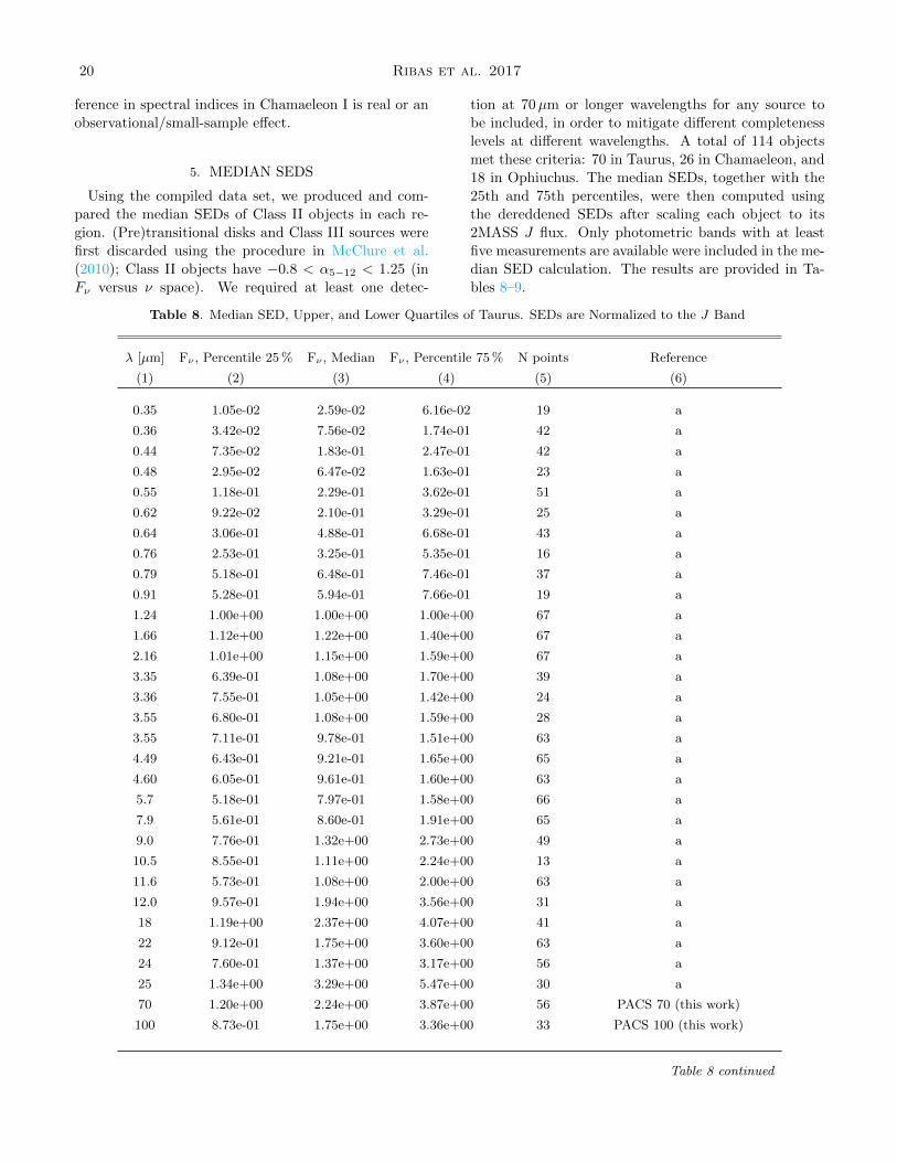
20 Ribas et al. 2017

ference in spectral indices in Chamaeleon I is real or an

observational/small-sample effect.

5. MEDIAN SEDS

Using the compiled data set, we produced and com-

pared the median SEDs of Class II objects in each re-

gion. (Pre)transitional disks and Class III sources were

first discarded using the procedure in McClure et al.

(2010); Class II objects have −0.8 < α5−12 < 1.25 (in

Fν versus ν space). We required at least one detec-

tion at 70µm or longer wavelengths for any source to

be included, in order to mitigate different completeness

levels at different wavelengths. A total of 114 objects

met these criteria: 70 in Taurus, 26 in Chamaeleon, and

18 in Ophiuchus. The median SEDs, together with the

25th and 75th percentiles, were then computed using

the dereddened SEDs after scaling each object to its

2MASS J flux. Only photometric bands with at least

five measurements are available were included in the me-

dian SED calculation. The results are provided in Ta-

bles 8–9.

Table 8. Median SED, Upper, and Lower Quartiles of Taurus. SEDs are Normalized to the J Band

λ [µm] Fν , Percentile 25 % Fν , Median Fν , Percentile 75 % N points Reference

(1) (2) (3) (4) (5) (6)

0.35 1.05e-02 2.59e-02 6.16e-02 19 a

0.36 3.42e-02 7.56e-02 1.74e-01 42 a

0.44 7.35e-02 1.83e-01 2.47e-01 42 a

0.48 2.95e-02 6.47e-02 1.63e-01 23 a

0.55 1.18e-01 2.29e-01 3.62e-01 51 a

0.62 9.22e-02 2.10e-01 3.29e-01 25 a

0.64 3.06e-01 4.88e-01 6.68e-01 43 a

0.76 2.53e-01 3.25e-01 5.35e-01 16 a

0.79 5.18e-01 6.48e-01 7.46e-01 37 a

0.91 5.28e-01 5.94e-01 7.66e-01 19 a

1.24 1.00e+00 1.00e+00 1.00e+00 67 a

1.66 1.12e+00 1.22e+00 1.40e+00 67 a

2.16 1.01e+00 1.15e+00 1.59e+00 67 a

3.35 6.39e-01 1.08e+00 1.70e+00 39 a

3.36 7.55e-01 1.05e+00 1.42e+00 24 a

3.55 6.80e-01 1.08e+00 1.59e+00 28 a

3.55 7.11e-01 9.78e-01 1.51e+00 63 a

4.49 6.43e-01 9.21e-01 1.65e+00 65 a

4.60 6.05e-01 9.61e-01 1.60e+00 63 a

5.7 5.18e-01 7.97e-01 1.58e+00 66 a

7.9 5.61e-01 8.60e-01 1.91e+00 65 a

9.0 7.76e-01 1.32e+00 2.73e+00 49 a

10.5 8.55e-01 1.11e+00 2.24e+00 13 a

11.6 5.73e-01 1.08e+00 2.00e+00 63 a

12.0 9.57e-01 1.94e+00 3.56e+00 31 a

18 1.19e+00 2.37e+00 4.07e+00 41 a

22 9.12e-01 1.75e+00 3.60e+00 63 a

24 7.60e-01 1.37e+00 3.17e+00 56 a

25 1.34e+00 3.29e+00 5.47e+00 30 a

70 1.20e+00 2.24e+00 3.87e+00 56 PACS 70 (this work)

100 8.73e-01 1.75e+00 3.36e+00 33 PACS 100 (this work)

Table 8 continued

Disks in Taurus, Ophiuchus, and Chamaeleon I 21

Table 8 (continued)

λ [µm] Fν , Percentile 25 % Fν , Median Fν , Percentile 75 % N points Reference

(1) (2) (3) (4) (5) (6)

160 1.00e+00 1.93e+00 3.86e+00 54 PACS 160 (this work)

250 9.33e-01 2.05e+00 4.25e+00 40 SPIRE 250 (this work)

350 1.49e+00 2.38e+00 3.70e+00 14 a

350 8.36e-01 1.63e+00 3.90e+00 35 SPIRE 350 (this work)

443 8.30e-01 1.29e+00 1.81e+00 13 a

450 1.29e+00 1.87e+00 2.71e+00 7 a

500 5.65e-01 1.21e+00 2.45e+00 30 SPIRE 500 (this work)

600 7.15e-01 8.97e-01 1.30e+00 6 a

624 7.60e-01 1.23e+00 2.16e+00 7 a

769 5.78e-01 8.46e-01 1.13e+00 13 a

800 3.42e-01 4.28e-01 6.26e-01 11 a

850 3.99e-01 6.40e-01 9.12e-01 6 a

869 6.80e-02 2.15e-01 4.53e-01 38 a

880 5.65e-02 1.36e-01 3.80e-01 17 a

1056 2.86e-01 3.93e-01 5.96e-01 15 a

1100 2.57e-01 2.70e-01 4.27e-01 6 a

1200 4.63e-02 1.67e-01 2.49e-01 10 a

1250 5.59e-02 1.82e-01 2.39e-01 27 a

1300 1.06e-01 1.87e-01 3.09e-01 18 a

1330 1.09e-01 2.56e-01 4.10e-01 14 a

1360 4.62e-02 6.91e-02 9.65e-02 7 PdBI1.36mm (Pietu et al. 2014)

2126 6.51e-02 7.64e-02 1.17e-01 5 a

2700 2.08e-02 3.60e-02 6.36e-02 17 a

2974 4.53e-03 7.50e-03 2.08e-02 5 a

Note—a: data from Andrews et al. (2013).

Table 9. Median SED, Upper, and Lower Quartiles of Chamaeleon. SEDs are Normalized to the J Band

λ [µm] Fν , Percentile 25 % Fν , Median Fν , Percentile 75 % N points Reference

(1) (2) (3) (4) (5) (6)

0.44 1.04e-01 1.73e-01 2.29e-01 17 B Johnson (APASS)

0.48 1.37e-01 1.86e-01 2.80e-01 18 g SDSS (APASS)

0.55 1.75e-01 2.65e-01 4.25e-01 17 V Johnson (APASS)

0.62 3.38e-01 3.93e-01 6.58e-01 17 r SDSS (APASS)

0.76 3.40e-01 4.67e-01 7.05e-01 17 i SDSS (APASS)

1.24 1.00e+00 1.00e+00 1.00e+00 26 2MASS J

1.66 1.25e+00 1.28e+00 1.39e+00 25 2MASS H

Table 9 continued

22 Ribas et al. 2017

Table 9 (continued)

λ [µm] Fν , Percentile 25 % Fν , Median Fν , Percentile 75 % N points Reference

(1) (2) (3) (4) (5) (6)

2.16 1.19e+00 1.26e+00 1.54e+00 25 2MASS K

3.35 7.87e-01 1.02e+00 1.69e+00 17 WISE 1

3.55 7.35e-01 9.43e-01 1.52e+00 18 IRAC 1

4.49 7.12e-01 8.97e-01 2.02e+00 19 IRAC 2

4.60 7.79e-01 1.06e+00 1.67e+00 18 WISE 2

5.7 5.81e-01 7.60e-01 2.14e+00 22 IRAC 3

7.9 6.14e-01 8.91e-01 2.42e+00 24 IRAC 4

9.0 8.62e-01 1.31e+00 2.45e+00 22 AKARI 9

11.6 8.52e-01 1.20e+00 2.15e+00 21 WISE 3

18 1.17e+00 1.75e+00 2.96e+00 20 AKARI 18

22 1.25e+00 1.68e+00 2.33e+00 21 WISE 4

24 1.03e+00 1.42e+00 2.05e+00 21 MIPS 1

70 1.37e+00 2.29e+00 5.94e+00 19 PACS 70 (this work)

100 1.35e+00 2.10e+00 4.70e+00 25 PACS 100 (this work)

160 1.12e+00 2.12e+00 2.78e+00 12 PACS 160 (this work)

250 4.83e-01 1.65e+00 2.04e+00 8 SPIRE 250 (this work)

350 1.12e+00 1.20e+00 1.94e+00 6 SPIRE 350 (this work)

500 5.08e-01 7.55e-01 1.41e+00 6 SPIRE 500 (this work)

870 9.35e-02 1.78e-01 3.02e-01 6 LABOCA 870 (Belloche et al. 2011)

887 4.42e-02 1.05e-01 2.53e-01 25 ALMA 887 (Pascucci et al. 2016)

Table 10. Median SED, Upper, and Lower Quartiles of Ophiuchus. SEDs are Normalized to the J Band

λ [µm] Fν , Percentile 25 % Fν , Median Fν , Percentile 75 % N points Reference

(1) (2) (3) (4) (5) (6)

0.44 7.59e-02 1.96e-01 2.21e-01 7 B Johnson (APASS)

0.48 1.12e-01 2.82e-01 3.12e-01 9 g SDSS (APASS)

0.55 1.50e-01 3.81e-01 4.18e-01 7 V Johnson (APASS)

0.62 2.58e-01 3.95e-01 4.83e-01 7 R CMC15

0.62 2.94e-01 5.12e-01 6.65e-01 9 r SDSS (APASS)

0.76 4.83e-01 5.68e-01 7.05e-01 8 i SDSS (APASS)

1.24 1.00e+00 1.00e+00 1.00e+00 18 2MASS J

1.66 1.11e+00 1.18e+00 1.22e+00 18 2MASS H

2.16 9.97e-01 1.07e+00 1.23e+00 18 2MASS K

3.35 6.80e-01 8.22e-01 1.01e+00 17 WISE 1

3.55 6.17e-01 8.07e-01 1.10e+00 14 IRAC 1

4.49 4.43e-01 6.68e-01 9.10e-01 16 IRAC 2

4.60 4.42e-01 6.99e-01 8.99e-01 17 WISE 2

Table 10 continued

Disks in Taurus, Ophiuchus, and Chamaeleon I 23

Table 10 (continued)

λ [µm] Fν , Percentile 25 % Fν , Median Fν , Percentile 75 % N points Reference

(1) (2) (3) (4) (5) (6)

5.7 3.70e-01 6.25e-01 7.60e-01 17 IRAC 3

7.9 4.62e-01 7.57e-01 9.44e-01 16 IRAC 4

9.0 7.86e-01 1.04e+00 1.44e+00 12 AKARI 9

11.6 5.04e-01 7.22e-01 1.15e+00 17 WISE 3

18 8.26e-01 1.15e+00 1.23e+00 7 AKARI 18

22 6.92e-01 1.22e+00 1.85e+00 16 WISE 4

24 7.98e-01 1.33e+00 1.73e+00 17 MIPS 1

70 4.39e-01 9.50e-01 2.83e+00 14 PACS 70 (this work)

100 6.68e-01 1.16e+00 2.93e+00 11 PACS 100 (this work)

160 7.65e-01 2.34e+00 2.58e+00 5 PACS 160 (this work)

250 2.86e-01 1.54e+00 3.11e+00 7 SPIRE 250 (this work)

850 6.09e-02 2.07e-01 9.00e-01 5 SCUBA 850 (Andrews & Williams 2007)

1300 2.46e-02 4.31e-02 2.36e-01 7 SCUBA 1300 (Andrews & Williams 2007)

3300 4.50e-03 1.06e-02 4.22e-02 6 ATCA 3.3 (Ricci et al. 2010a)

The obtained SEDs are shown in Fig. 11. We found

them to be identical within the quartiles down to the

(sub)mm regime. This comparison expands the result

in Furlan et al. (2009), where the median IRS spec-

tra of Taurus, Chamaeleon, and Ophiuchus were already

found to be very similar. This is somewhat surprising,

given that the three regions have different ages and more

evolved disks are expected in Chamaeleon I than in Tau-

rus and Ophiuchus. Additionally, the extent of the up-

per and lower quartiles also appear to be similar for the

three regions, suggesting a similar spread in disk mor-

phologies in the three regions. We speculate that the

intrinsic scatter in disk morphologies, together with the

selection of Class II disks formerly applied (which effec-

tively includes disks with certain spectral indices only),

may erase existing trends with age. Including objects

classified as (pre)transitional disks does not change this

result, but the median SEDs compiled here do not in-

clude Class III or diskless sources; thus, they represent

the typical SED of disks in the regions more so than

the median SED of all objects. We also note that our

sample is not complete, and these median SEDs are bi-

ased toward bright objects. Despite this, the lack of

differences between the estimated medians, combined

with the similar median IRS spectra of these associa-

tions, suggest that either Class II disks have very sim-

ilar structures/properties in different star-forming re-

gions (at least to the extent traceable with SEDs), or

the intrinsic variations in their morphologies are broad

enough to create a “typical protoplanetary disk” SED.

High-resolution observations have often revealed com-

plex structures in disks, such as multiple rings, spiral

arms, or dust traps (e.g. Muto et al. 2012; van der Marel

et al. 2013; ALMA Partnership et al. 2015), favoring

the second explanation, but the number of objects per

region is still significantly small, particularly in Ophi-

uchus and Chamaeleon. Future surveys of large samples

of disks, especially in the (sub)mm regime, will produce

more complete and sensitive median SEDs, which may

reveal unseen region-to-region differences and shed some

light on the “typical” median SED of protoplanetary

disks. For comparison, in Fig. 11 we also include the

median SED of K/M-type stars in the Upper Scorpius

(Upper Sco) region from Mathews et al. (2013). The ab-

solute age of this region is still under debate, but there is

strong evidence for Upper Sco being older than Taurus,

Chamaeleon I, and Ophiuchus (4-13 Myr, e.g. Preibisch

et al. 2002; Pecaut et al. 2012; Herczeg & Hillenbrand

2015). Although the optical part of the SEDs cannot

be directly compared due to the different treatment in

Mathews et al. (2013), the median SED of Upper Sco

shows a deficit of near/mid-IR excess with respect to

the younger ones, indicating that disks in Upper Sco

are more evolved (e.g. more settled). In the future, ex-

tending the median SED of disks in Upper Sco to longer

wavelengths will enable one to search for evidence of

dust growth signatures in such older regions.

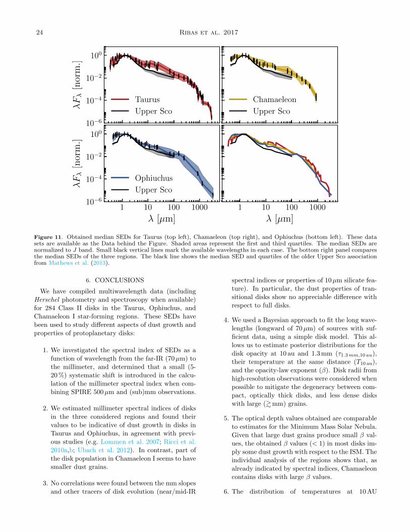
24 Ribas et al. 2017

1 10 100 1000

λ [µm]

10−6

10−4

10−2

100

λFλ

[nor

m.]

Taurus

Upper Sco

Chamaeleon

Upper Sco

1 10 100 1000

λ [µm]

10−6

10−4

10−2

100

λFλ

[nor

m.]

Ophiuchus

Upper Sco

Figure 11. Obtained median SEDs for Taurus (top left), Chamaeleon (top right), and Ophiuchus (bottom left). These datasets are available as the Data behind the Figure. Shaded areas represent the first and third quartiles. The median SEDs arenormalized to J band. Small black vertical lines mark the available wavelengths in each case. The bottom right panel comparesthe median SEDs of the three regions. The black line shows the median SED and quartiles of the older Upper Sco associationfrom Mathews et al. (2013).

6. CONCLUSIONS

We have compiled multiwavelength data (including

Herschel photometry and spectroscopy when available)

for 284 Class II disks in the Taurus, Ophiuchus, and

Chamaeleon I star-forming regions. These SEDs have

been used to study different aspects of dust growth and

properties of protoplanetary disks:

1. We investigated the spectral index of SEDs as a

function of wavelength from the far-IR (70µm) to

the millimeter, and determined that a small (5-

20 %) systematic shift is introduced in the calcu-

lation of the millimeter spectral index when com-

bining SPIRE 500µm and (sub)mm observations.

2. We estimated millimeter spectral indices of disks

in the three considered regions and found their

values to be indicative of dust growth in disks in

Taurus and Ophiuchus, in agreement with previ-

ous studies (e.g. Lommen et al. 2007; Ricci et al.

2010a,b; Ubach et al. 2012). In contrast, part of

the disk population in Chamaeleon I seems to have

smaller dust grains.

3. No correlations were found between the mm slopes

and other tracers of disk evolution (near/mid-IR

spectral indices or properties of 10µm silicate fea-

ture). In particular, the dust properties of tran-

sitional disks show no appreciable difference with

respect to full disks.

4. We used a Bayesian approach to fit the long wave-

lengths (longward of 70µm) of sources with suf-

ficient data, using a simple disk model. This al-

lows us to estimate posterior distributions for the

disk opacity at 10 au and 1.3 mm (τ1.3mm,10 au),

their temperature at the same distance (T10 au),

and the opacity-law exponent (β). Disk radii from

high-resolution observations were considered when

possible to mitigate the degeneracy between com-

pact, optically thick disks, and less dense disks

with large (&mm) grains.

5. The optical depth values obtained are comparable

to estimates for the Minimum Mass Solar Nebula.

Given that large dust grains produce small β val-

ues, the obtained β values (< 1) in most disks im-

ply some dust growth with respect to the ISM. The

individual analysis of the regions shows that, as

already indicated by spectral indices, Chamaeleon

contains disks with large β values.

6. The distribution of temperatures at 10 AU

Disks in Taurus, Ophiuchus, and Chamaeleon I 25

(T10 AU) peaks around 40-50 K and shows no signif-

icant difference among regions. A strong correla-

tion of this parameter with observed 70µm fluxes

is also found.

7. There is evidence for a different distribution of

spectral indices and βs in Taurus and Ophiuchus

with respect to Chamaeleon I, the latter having

steeper values. If this difference in spectral indices

is caused by its older age, then the high millimeter

fluxes of its disks require that they were initially

more massive than their Taurus/Ophiuchus coun-

terparts. After inspecting their location in the HR

diagram, we find that a bias toward the youngest

sources cannot explain all the steep slopes. Given

the small number of sources with millimeter spec-

tral index measurements in Chamaeleon I, this re-

sult should be confirmed with a larger sample.

8. We built the median SED of protoplanetary disks

in each region and found them to be indistinguish-

able down to mm wavelengths within their quar-

tiles, suggesting that either disks are quite similar

in these associations or they display such a large

variety of morphologies that produces a “typical”

median SED.

Some of these results are tentative due to the small

sample sizes, despite the large data compilation pre-

sented here. Future (sub)mm surveys of disks, especially

in Ophiuchus and Chamaeleon I, will be critical to ob-

tain better estimates of spectral indices at these wave-

lengths and, in particular, determine the origin of the

apparently different spectral indices in Chamaeleon I.

Additionally, analyzing the compiled data with detailed

disk models such as the ones presented in D’Alessio et al.(1998, 1999, 2001, 2006), especially when combined with

a Bayesian approach, will inform us of important pro-

cesses such as the dust settling.

We thank the referee for their thorough review and

comments that helped improve the quality of this

manuscript. We also thank Melissa McClure and Manoj

Puravankara for providing IRS spectra of objects in

Ophiuchus and Chamaeleon, and Greg Schwarz for help-

ing with the data formatting. This material is based

upon work supported by the National Science Foun-

dation under Grant No. AST-1455042. It is also

funded by Herschel Grant No. JPL RSA 1500040.

D.A.N. and M.H.D.vdW. acknowledge support from

the CSA and NSERC. PACS has been developed by a

consortium of institutes led by MPE (Germany) and

including UVIE (Austria); KU Leuven, CSL, IMEC

(Belgium); CEA, LAM (France); MPIA (Germany);

INAF-IFSI/OAA/OAP/OAT, LENS, SISSA (Italy);

IAC (Spain). This development has been supported by

the funding agencies BMVIT (Austria), ESA-PRODEX

(Belgium), CEA/CNES (France), DLR (Germany),

ASI/INAF (Italy), and CICYT/MCYT (Spain). SPIRE

has been developed by a consortium of institutes led

by Cardiff University (UK) and including Univ. Leth-

bridge (Canada); NAOC (China); CEA, LAM (France);

IFSI, Univ. Padua (Italy); IAC (Spain); Stockholm

Observatory (Sweden); Imperial College London, RAL,

UCL-MSSL, UKATC, Univ. Sussex (UK); and Cal-

tech, JPL, NHSC, Univ. Colorado (USA). This devel-

opment has been supported by national funding agen-

cies: CSA (Canada); NAOC (China); CEA, CNES,

CNRS (France); ASI (Italy); MCINN (Spain); SNSB

(Sweden); STFC, UKSA (UK); and NASA (USA). The

CMC15 Data Access Service is the result of a collabo-

ration agreement between the Centro de Astrobiologıa

(CAB, INTA-CSIC) and the Real Instituto y Observa-

torio de la Armada en San Fernando (ROA). It has been

developed in the framework of the Spanish Virtual Ob-

servatory project, supported by the Spanish MINECO

through grant AYA 2011-14052 and the CoSADIE FP7

project (Call INFRA-2012-3.3 Research Infrastructures,

project 312559). The system is maintained by the Data

Archive Unit of the CAB (CSIC -INTA). Based on

data from CMC15 Data Access Service at CAB (INTA-

CSIC). Funding for SDSS-III has been provided by the

Alfred P. Sloan Foundation, the Participating Institu-

tions, the National Science Foundation, and the U.S. De-

partment of Energy Office of Science. The SDSS-III web

site is http://www.sdss3.org/. SDSS-III is managed by

the Astrophysical Research Consortium for the Partici-

pating Institutions of the SDSS-III Collaboration includ-

ing the University of Arizona, the Brazilian Participa-

tion Group, Brookhaven National Laboratory, Carnegie

Mellon University, University of Florida, the French

Participation Group, the German Participation Group,

Harvard University, the Instituto de Astrofisica de Ca-

narias, the Michigan State/Notre Dame/JINA Partic-

ipation Group, Johns Hopkins University, Lawrence

Berkeley National Laboratory, Max Planck Institute for

Astrophysics, Max Planck Institute for Extraterrestrial

Physics, New Mexico State University, New York Uni-

versity, Ohio State University, Pennsylvania State Uni-

versity, University of Portsmouth, Princeton University,

the Spanish Participation Group, University of Tokyo,

University of Utah, Vanderbilt University, University of

Virginia, University of Washington, and Yale University.

Software: HIPE v14 (Ott 2010), emcee (Foreman-

Mackey et al. 2013), Matplotlib (Hunter 2007), SciPy

(Jones et al. 2001), Numpy (van der Walt et al. 2011),

pandas (Jones et al. 2001)

26 Ribas et al. 2017

REFERENCES

Adachi, I., Hayashi, C., & Nakazawa, K. 1976, Progress of

Theoretical Physics, 56, 1756

Ahn, C. P., Alexandroff, R., Allende Prieto, C., et al. 2012,

ApJS, 203, 21

Alexander, R., Pascucci, I., Andrews, S., Armitage, P., & Cieza,

L. 2014, Protostars and Planets VI, 475

Allard, F., Homeier, D., & Freytag, B. 2012, Royal Society of

London Philosophical Transactions Series A, 370, 2765

ALMA Partnership, Brogan, C. L., Perez, L. M., et al. 2015,

ApJL, 808, L3

Andre, P., & Montmerle, T. 1994, ApJ, 420, 837

Andre, P., Men’shchikov, A., Bontemps, S., et al. 2010, A&A,

518, L102

Andrews, S. M., Rosenfeld, K. A., Kraus, A. L., & Wilner, D. J.

2013, ApJ, 771, 129

Andrews, S. M., & Williams, J. P. 2005, ApJ, 631, 1134

—. 2007, ApJ, 671, 1800

Andrews, S. M., Wilner, D. J., Espaillat, C., et al. 2011, ApJ,

732, 42

Andrews, S. M., Wilner, D. J., Hughes, A. M., Qi, C., &

Dullemond, C. P. 2010, ApJ, 723, 1241

Baraffe, I., Homeier, D., Allard, F., & Chabrier, G. 2015, A&A,

577, A42

Beckwith, S. V. W., & Sargent, A. I. 1991, ApJ, 381, 250

Beckwith, S. V. W., Sargent, A. I., Chini, R. S., & Guesten, R.

1990, AJ, 99, 924

Belloche, A., Schuller, F., Parise, B., et al. 2011, A&A, 527, A145

Birnstiel, T., Dullemond, C. P., & Brauer, F. 2010, A&A, 513,

A79

Brauer, F., Dullemond, C. P., Johansen, A., et al. 2007, A&A,

469, 1169

Brown, J. M., Blake, G. A., Dullemond, C. P., et al. 2007, ApJL,

664, L107

Bustamante, I., Merın, B., Ribas, A., et al. 2015, A&A, 578, A23

Calvet, N., D’Alessio, P., Hartmann, L., et al. 2002, ApJ, 568,

1008

Calvet, N., Magris, G. C., Patino, A., & D’Alessio, P. 1992,

RMxAA, 24, 27

Chiang, E. I., & Goldreich, P. 1997, ApJ, 490, 368

Cieza, L. A., Olofsson, J., Harvey, P. M., et al. 2013, ApJ, 762,

100

D’Alessio, P., Calvet, N., & Hartmann, L. 2001, ApJ, 553, 321

D’Alessio, P., Calvet, N., Hartmann, L., Franco-Hernandez, R.,

& Servın, H. 2006, ApJ, 638, 314

D’Alessio, P., Calvet, N., Hartmann, L., Lizano, S., & Canto, J.

1999, ApJ, 527, 893

D’Alessio, P., Canto, J., Calvet, N., & Lizano, S. 1998, ApJ, 500,

411

Davis, S. S. 2005, ApJL, 627, L153

Dent, W. R. F., Thi, W. F., Kamp, I., et al. 2013, PASP, 125,

477

Draine, B. T. 2006, ApJ, 636, 1114

Dullemond, C. P., Dominik, C., & Natta, A. 2001, ApJ, 560, 957

Dzib, S. A., Loinard, L., Mioduszewski, A. J., et al. 2013, ApJ,

775, 63

Espaillat, C., Furlan, E., D’Alessio, P., et al. 2011, ApJ, 728, 49

Espaillat, C., Muzerolle, J., Najita, J., et al. 2014, Protostars

and Planets VI, 497

Evans, II, N. J., Dunham, M. M., Jørgensen, J. K., et al. 2009,

ApJS, 181, 321

Foreman-Mackey, D., Hogg, D. W., Lang, D., & Goodman, J.

2013, PASP, 125, 306

Forrest, W. J., Sargent, B., Furlan, E., et al. 2004, ApJS, 154,

443

Fulton, T., Naylor, D. A., Polehampton, E. T., et al. 2016,

MNRAS, 458, 1977

Furlan, E., Calvet, N., D’Alessio, P., et al. 2005, ApJL, 628, L65

Furlan, E., Hartmann, L., Calvet, N., et al. 2006, ApJS, 165, 568

Furlan, E., Watson, D. M., McClure, M. K., et al. 2009, ApJ,

703, 1964

Furlan, E., Luhman, K. L., Espaillat, C., et al. 2011, The

Astrophysical Journal Supplement Series, 195, 3

Goodman, J., & Weare, J. 2010, Comm. App. Math. Comp. Sci.,

5, 65

Gracia-Carpio, J., Wetzstein, M., & Roussel, H. 2015, ArXiv

e-prints, arXiv:1512.03252

Guilloteau, S., Pietu, V., Chapillon, E., et al. 2016, A&A, 586, L1

Haisch, Jr., K. E., Lada, E. A., & Lada, C. J. 2001, ApJL, 553,

L153

Henden, A. A., Templeton, M., Terrell, D., et al. 2016, VizieR

Online Data Catalog, 2336

Henning, T., Pfau, W., Zinnecker, H., & Prusti, T. 1993, A&A,

276, 129

Herczeg, G. J., & Hillenbrand, L. A. 2015, ApJ, 808, 23

Hernandez, J., Calvet, N., Briceno, C., et al. 2007, ApJ, 671,

1784

Hildebrand, R. H. 1983, QJRAS, 24, 267

Houck, J. R., Roellig, T. L., van Cleve, J., et al. 2004, ApJS,

154, 18

Howard, C. D., Sandell, G., Vacca, W. D., et al. 2013, ApJ, 776,

21

Hunter, J. D. 2007, Computing In Science & Engineering, 9, 90

Ireland, M. J., & Kraus, A. L. 2008, ApJL, 678, L59

Ishihara, D., Onaka, T., Kataza, H., et al. 2010, A&A, 514, A1+

Jones, E., Oliphant, T., Peterson, P., et al. 2001, SciPy: Open

source scientific tools for Python, , , [Online; accessed ¡today¿]

Kenyon, S. J., & Hartmann, L. 1987, ApJ, 323, 714

Kessler-Silacci, J., Augereau, J.-C., Dullemond, C. P., et al.

2006, ApJ, 639, 275

Lebouteiller, V., Barry, D. J., Goes, C., et al. 2015, ApJS, 218,

21

Lebouteiller, V., Barry, D. J., Spoon, H. W. W., et al. 2011,

ApJS, 196, 8

Lommen, D., Wright, C. M., Maddison, S. T., et al. 2007, A&A,

462, 211

Lommen, D. J. P., van Dishoeck, E. F., Wright, C. M., et al.

2010, A&A, 515, A77

Luhman, K. L. 2007, ApJS, 173, 104

Luhman, K. L., Allen, L. E., Allen, P. R., et al. 2008, ApJ, 675,

1375

Manoj, P., Kim, K. H., Furlan, E., et al. 2011, ApJS, 193, 11

Marchili, N., Hopwood, R., Fulton, T., et al. 2017, MNRAS, 464,

3331

Mathews, G. S., Pinte, C., Duchene, G., Williams, J. P., &

Menard, F. 2013, A&A, 558, A66

Mathis, J. S. 1990, ARA&A, 28, 37

Mathis, J. S., Rumpl, W., & Nordsieck, K. H. 1977, ApJ, 217,

425

McClure, M. 2009, ApJL, 693, L81

McClure, M. K., Furlan, E., Manoj, P., et al. 2010, ApJS, 188, 75

Merın, B., Brown, J. M., Oliveira, I., et al. 2010, ApJ, 718, 1200

Miyake, K., & Nakagawa, Y. 1993, Icarus, 106, 20

Morales-Calderon, M., Stauffer, J. R., Hillenbrand, L. A., et al.

2011, ApJ, 733, 50

Murakami, H., Baba, H., Barthel, P., et al. 2007, PASJ, 59, 369

Muto, T., Grady, C. A., Hashimoto, J., et al. 2012, ApJL, 748,

L22

Muzerolle, J., Calvet, N., Hartmann, L., & D’Alessio, P. 2003,

ApJL, 597, L149

Disks in Taurus, Ophiuchus, and Chamaeleon I 27

Natta, A., Testi, L., Calvet, N., et al. 2007, Protostars and

Planets V, 767Natta, A., Testi, L., Neri, R., Shepherd, D. S., & Wilner, D. J.

2004, A&A, 416, 179

Olofsson, J., Szucs, L., Henning, T., et al. 2013, A&A, 560, A100Ortiz-Leon, G. N., Loinard, L., Kounkel, M. A., et al. 2017, ApJ,

834, 141Osorio, M., Macıas, E., Anglada, G., et al. 2016, ApJL, 825, L10

Ott, S. 2010, in Astronomical Society of the Pacific Conference

Series, Vol. 434, Astronomical Data Analysis Software andSystems XIX, ed. Y. Mizumoto, K.-I. Morita, & M. Ohishi, 139

Pascucci, I., Gorti, U., & Hollenbach, D. 2012, ApJL, 751, L42

Pascucci, I., Testi, L., Herczeg, G. J., et al. 2016, ApJ, 831, 125Pearson, C., Lim, T., North, C., et al. 2014, Experimental

Astronomy, 37, 175

Pecaut, M. J., & Mamajek, E. E. 2013, ApJS, 208, 9Pecaut, M. J., Mamajek, E. E., & Bubar, E. J. 2012, ApJ, 746,

154

Pietu, V., Guilloteau, S., Di Folco, E., Dutrey, A., & Boehler, Y.2014, A&A, 564, A95

Pilbratt, G. L., Riedinger, J. R., Passvogel, T., et al. 2010, A&A,518, L1

Pinilla, P., Birnstiel, T., Ricci, L., et al. 2012, A&A, 538, A114

Preibisch, T., Brown, A. G. A., Bridges, T., Guenther, E., &Zinnecker, H. 2002, AJ, 124, 404

Rebollido, I., Merın, B., Ribas, A., et al. 2015, A&A, 581, A30

Ribas, A., Bouy, H., & Merın, B. 2015, A&A, 576, A52Ribas, A., Merın, B., Bouy, H., et al. 2013, A&A, 552, A115

Ricci, L., Testi, L., Natta, A., & Brooks, K. J. 2010a, A&A, 521,

A66Ricci, L., Testi, L., Natta, A., et al. 2010b, A&A, 512, A15

—. 2014, ApJ, 791, 20

Riviere-Marichalar, P., Merın, B., Kamp, I., Eiroa, C., &Montesinos, B. 2016, A&A, 594, A59

Rodmann, J., Henning, T., Chandler, C. J., Mundy, L. G., &Wilner, D. J. 2006, A&A, 446, 211

Siess, L., Dufour, E., & Forestini, M. 2000, A&A, 358, 593

Skrutskie, M. F., Cutri, R. M., Stiening, R., et al. 2006, The

Astronomical Journal, 131, 1163

Spezzi, L., Cox, N. L. J., Prusti, T., et al. 2013, A&A, 555, A71

Strom, K. M., Strom, S. E., Edwards, S., Cabrit, S., & Skrutskie,

M. F. 1989, AJ, 97, 1451

Takeuchi, T., & Lin, D. N. C. 2002, ApJ, 581, 1344

—. 2005, ApJ, 623, 482

Testi, L., Natta, A., Scholz, A., et al. 2016, A&A, 593, A111

Testi, L., Birnstiel, T., Ricci, L., et al. 2014, Protostars and

Planets VI, 339

Torres, R. M., Loinard, L., Mioduszewski, A. J., & Rodrıguez,

L. F. 2007, ApJ, 671, 1813

Ubach, C., Maddison, S. T., Wright, C. M., et al. 2012, MNRAS,

425, 3137

Valtchanov, I., Hopwood, R., Polehampton, E., et al. 2014,

Experimental Astronomy, 37, 207

van der Marel, N., van Dishoeck, E. F., Bruderer, S., et al. 2013,

Science, 340, 1199

van der Plas, G., Wright, C. M., Menard, F., et al. 2017, A&A,

597, A32

van der Walt, S., Colbert, S. C., & Varoquaux, G. 2011,

Computing in Science Engineering, 13, 22

Walsh, C., Juhasz, A., Meeus, G., et al. 2016, ApJ, 831, 200

Weidenschilling, S. J. 1977, Ap&SS, 51, 153

Whittet, D. C. B., Prusti, T., Franco, G. A. P., et al. 1997,

A&A, 327, 1194

Wilking, B. A., Gagne, M., & Allen, L. E. 2008, Star Formation

in the ρ Ophiuchi Molecular Cloud, ed. B. Reipurth, 351

Winston, E., Cox, N. L. J., Prusti, T., et al. 2012, A&A, 545,

A145

Wright, E. L., Eisenhardt, P. R. M., Mainzer, A. K., et al. 2010,

The Astronomical Journal, 140, 1868

Zhu, Z., Nelson, R. P., Hartmann, L., Espaillat, C., & Calvet, N.

2011, ApJ, 729, 47

APPENDIX

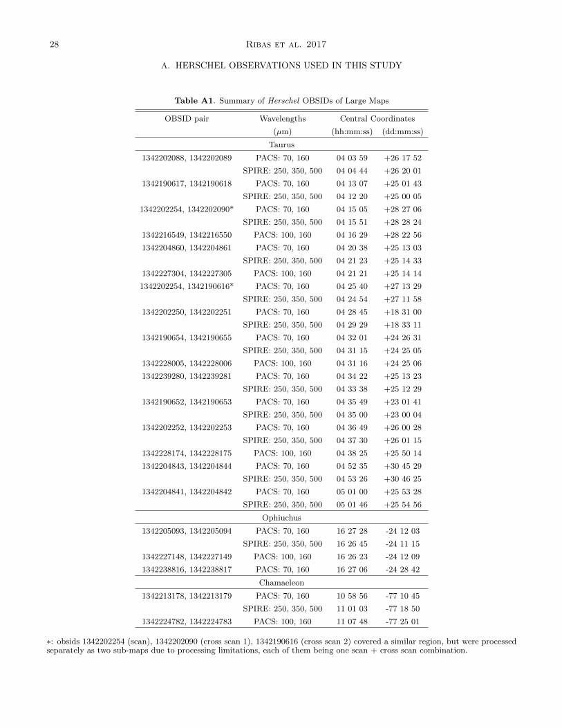
28 Ribas et al. 2017

A. HERSCHEL OBSERVATIONS USED IN THIS STUDY

Table A1. Summary of Herschel OBSIDs of Large Maps

OBSID pair Wavelengths Central Coordinates

(µm) (hh:mm:ss) (dd:mm:ss)

Taurus

1342202088, 1342202089 PACS: 70, 160 04 03 59 +26 17 52

SPIRE: 250, 350, 500 04 04 44 +26 20 01

1342190617, 1342190618 PACS: 70, 160 04 13 07 +25 01 43

SPIRE: 250, 350, 500 04 12 20 +25 00 05

1342202254, 1342202090* PACS: 70, 160 04 15 05 +28 27 06

SPIRE: 250, 350, 500 04 15 51 +28 28 24

1342216549, 1342216550 PACS: 100, 160 04 16 29 +28 22 56

1342204860, 1342204861 PACS: 70, 160 04 20 38 +25 13 03

SPIRE: 250, 350, 500 04 21 23 +25 14 33

1342227304, 1342227305 PACS: 100, 160 04 21 21 +25 14 14

1342202254, 1342190616* PACS: 70, 160 04 25 40 +27 13 29

SPIRE: 250, 350, 500 04 24 54 +27 11 58

1342202250, 1342202251 PACS: 70, 160 04 28 45 +18 31 00

SPIRE: 250, 350, 500 04 29 29 +18 33 11

1342190654, 1342190655 PACS: 70, 160 04 32 01 +24 26 31

SPIRE: 250, 350, 500 04 31 15 +24 25 05

1342228005, 1342228006 PACS: 100, 160 04 31 16 +24 25 06

1342239280, 1342239281 PACS: 70, 160 04 34 22 +25 13 23

SPIRE: 250, 350, 500 04 33 38 +25 12 29

1342190652, 1342190653 PACS: 70, 160 04 35 49 +23 01 41

SPIRE: 250, 350, 500 04 35 00 +23 00 04

1342202252, 1342202253 PACS: 70, 160 04 36 49 +26 00 28

SPIRE: 250, 350, 500 04 37 30 +26 01 15

1342228174, 1342228175 PACS: 100, 160 04 38 25 +25 50 14

1342204843, 1342204844 PACS: 70, 160 04 52 35 +30 45 29

SPIRE: 250, 350, 500 04 53 26 +30 46 25

1342204841, 1342204842 PACS: 70, 160 05 01 00 +25 53 28

SPIRE: 250, 350, 500 05 01 46 +25 54 56

Ophiuchus

1342205093, 1342205094 PACS: 70, 160 16 27 28 -24 12 03

SPIRE: 250, 350, 500 16 26 45 -24 11 15

1342227148, 1342227149 PACS: 100, 160 16 26 23 -24 12 09

1342238816, 1342238817 PACS: 70, 160 16 27 06 -24 28 42

Chamaeleon

1342213178, 1342213179 PACS: 70, 160 10 58 56 -77 10 45

SPIRE: 250, 350, 500 11 01 03 -77 18 50

1342224782, 1342224783 PACS: 100, 160 11 07 48 -77 25 01

∗: obsids 1342202254 (scan), 1342202090 (cross scan 1), 1342190616 (cross scan 2) covered a similar region, but were processedseparately as two sub-maps due to processing limitations, each of them being one scan + cross scan combination.

Disks in Taurus, Ophiuchus, and Chamaeleon I 29

Table A2. Additional Herschel Observations of Sources Outside Large Maps

Object OBSIDs Wavelengths Object Coordinates

(µm) (hh:mm:ss) (dd:mm:ss)

2MASS J04390525+2337450 1342243086, 1342243087 70, 160 04 39 05 +23 37 45

2MASS J04393364+2359212 1342243438, 1342243439 70, 160 04 39 34 +23 59 21

2MASS J04400067+2358211 1342243436, 1342243437 70, 160 04 40 01 +23 58 21

CoKu Tau/4 1342193136 70, 160* 04 41 17 +28 40 00

1342217520, 1342217521 100, 160*

CX Tau 1342216545, 1342216546 70, 160 04 14 48 +26 48 11

1342216547, 1342216548 100, 160

DQ Tau 1342217462, 1342217463 70, 160 04 46 53 +17 00 00

1342217464, 1342217465 100, 160

DS Tau 1342193135 70, 160 04 47 49 +29 25 11

1342217518, 1342217519 100, 160

FP Tau 1342216545, 1342216546 70, 160 04 14 47 +26 46 26

1342216547, 1342216548 100, 160

Haro 6-37 1342193141 70, 160 04 46 59 +17 02 38

1342217466, 1342217467 100, 160

LkCa 15 1342217470, 1342217471 70, 160 04 39 18 +22 21 04

1342217472, 1342217473 100, 160

RW Aur 1342193130 70, 160 05 07 50 +30 24 05

1342217508, 1342217509 100, 160

∗: 160 µm flux measurements were discarded in the case of CoKu/Tau 4 due to extended emission.

Note—For single observations, only one OBSID is listed.

Table A3. SPIRE FTS spectra Used

(after Quality Check)

Name OBSIDs

16156-2358AB 1342242600

16201-2410 1342262850

AA Tau 1342265818

CI Tau 1342265815

CR Cha 1342257313

CS Cha 1342257315

CU Cha 1342224750

CW Tau 1342249051

DG Tau 1342265852

DL Tau 1342265849

DOAR25 1342262851

DQ Tau 1342228736

DR Tau 1342243598

GG Tau 1342265813

GM Aur 1342228740

Haro 6-37 1342228737

Table A3 continued

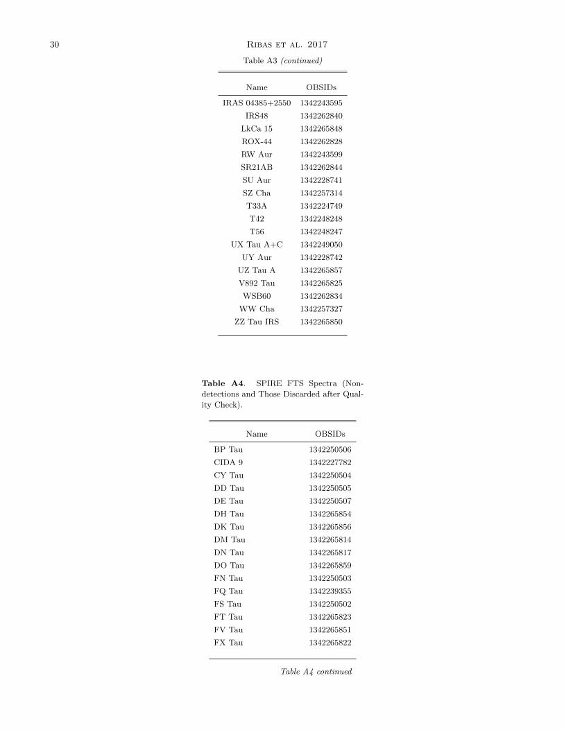
30 Ribas et al. 2017

Table A3 (continued)

Name OBSIDs

IRAS 04385+2550 1342243595

IRS48 1342262840

LkCa 15 1342265848

ROX-44 1342262828

RW Aur 1342243599

SR21AB 1342262844

SU Aur 1342228741

SZ Cha 1342257314

T33A 1342224749

T42 1342248248

T56 1342248247

UX Tau A+C 1342249050

UY Aur 1342228742

UZ Tau A 1342265857

V892 Tau 1342265825

WSB60 1342262834

WW Cha 1342257327

ZZ Tau IRS 1342265850

Table A4. SPIRE FTS Spectra (Non-

detections and Those Discarded after Qual-

ity Check).

Name OBSIDs

BP Tau 1342250506

CIDA 9 1342227782

CY Tau 1342250504

DD Tau 1342250505

DE Tau 1342250507

DH Tau 1342265854

DK Tau 1342265856

DM Tau 1342265814

DN Tau 1342265817

DO Tau 1342265859

FN Tau 1342250503

FQ Tau 1342239355

FS Tau 1342250502

FT Tau 1342265823

FV Tau 1342265851

FX Tau 1342265822

Table A4 continued

Disks in Taurus, Ophiuchus, and Chamaeleon I 31

Table A4 (continued)

Name OBSIDs

GH Tau 1342250496

GI Tau 1342250498

GK Tau 1342265819

GO Tau 1342243597

Haro 6-13 1342265820

GY314 1342262838

HK Tau 1342265821

HP Tau 1342227449

IRAS 04154+2823 1342265826

IRAS 04216+2603 1342250501

IRAS 04260+2642 1342265853

IP Tau 1342265824

IQ Tau 1342265855

MHO 3 1342249052

V710 Tau 1342250495

V807 Tau 1342250497

V836 Tau 1342227783

16193-2314 1342251283

DOAR16AB 1342262825

16225-2607 1342262853

DOAR21 1342262849

DOAR24 1342262848

GSS39 1342262846

DOAR28 1342262824

IRS49 1342262839

GY314 1342262838

16289-2457 1342262833

ROX-43A1 1342262829

SX Cha 1342251309

TW Cha 1342248245

CT Cha 1342231974

ISO 52 1342257316

T21 1342257318

CHXR 20 1342231082

UY Cha 1342257319

UZ Cha 1342257332

CHXR 22E 1342251310

T25 1342231973

CHXR 30B 1342257320

VW Cha 1342224752

T35 1342257321

VZ Cha 1342257331

C7-1 1342231081

Table A4 continued

32 Ribas et al. 2017

Table A4 (continued)

Name OBSIDs

B43 1342231080

T43 1342257330

WX Cha 1342257317

WY Cha 1342257329

Hn 11 1342257328

T47 1342257322

WZ Cha 1342257326

XX Cha 1342251291

T51 1342257325

CV Cha 1342257324

T54 1342257323

2M J11241186-7630425 1342243638

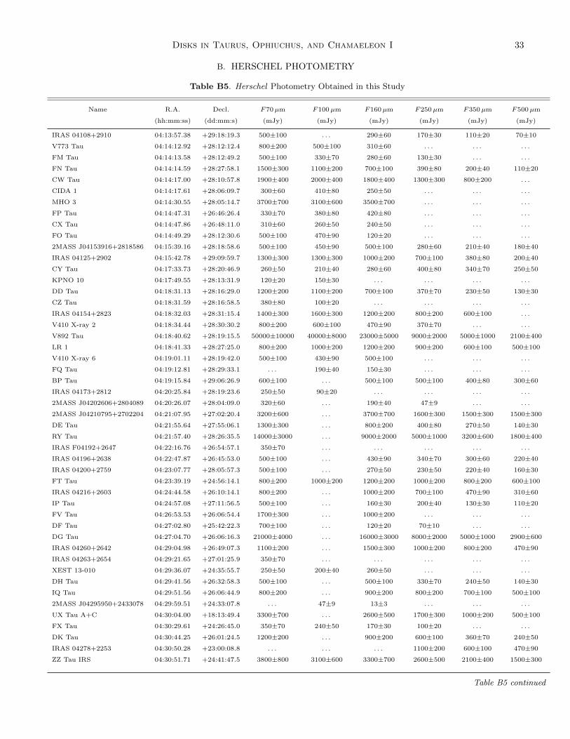
Disks in Taurus, Ophiuchus, and Chamaeleon I 33

B. HERSCHEL PHOTOMETRY

Table B5. Herschel Photometry Obtained in this Study

Name R.A. Decl. F70µm F100µm F160µm F250µm F350µm F500µm

(hh:mm:ss) (dd:mm:s) (mJy) (mJy) (mJy) (mJy) (mJy) (mJy)

IRAS 04108+2910 04:13:57.38 +29:18:19.3 500±100 . . . 290±60 170±30 110±20 70±10

V773 Tau 04:14:12.92 +28:12:12.4 800±200 500±100 310±60 . . . . . . . . .

FM Tau 04:14:13.58 +28:12:49.2 500±100 330±70 280±60 130±30 . . . . . .

FN Tau 04:14:14.59 +28:27:58.1 1500±300 1100±200 700±100 390±80 200±40 110±20

CW Tau 04:14:17.00 +28:10:57.8 1900±400 2000±400 1800±400 1300±300 800±200 . . .

CIDA 1 04:14:17.61 +28:06:09.7 300±60 410±80 250±50 . . . . . . . . .

MHO 3 04:14:30.55 +28:05:14.7 3700±700 3100±600 3500±700 . . . . . . . . .

FP Tau 04:14:47.31 +26:46:26.4 330±70 380±80 420±80 . . . . . . . . .

CX Tau 04:14:47.86 +26:48:11.0 310±60 260±50 240±50 . . . . . . . . .

FO Tau 04:14:49.29 +28:12:30.6 500±100 470±90 120±20 . . . . . . . . .

2MASS J04153916+2818586 04:15:39.16 +28:18:58.6 500±100 450±90 500±100 280±60 210±40 180±40

IRAS 04125+2902 04:15:42.78 +29:09:59.7 1300±300 1300±300 1000±200 700±100 380±80 200±40

CY Tau 04:17:33.73 +28:20:46.9 260±50 210±40 280±60 400±80 340±70 250±50

KPNO 10 04:17:49.55 +28:13:31.9 120±20 150±30 . . . . . . . . . . . .

DD Tau 04:18:31.13 +28:16:29.0 1200±200 1100±200 700±100 370±70 230±50 130±30

CZ Tau 04:18:31.59 +28:16:58.5 380±80 100±20 . . . . . . . . . . . .

IRAS 04154+2823 04:18:32.03 +28:31:15.4 1400±300 1600±300 1200±200 800±200 600±100 . . .

V410 X-ray 2 04:18:34.44 +28:30:30.2 800±200 600±100 470±90 370±70 . . . . . .

V892 Tau 04:18:40.62 +28:19:15.5 50000±10000 40000±8000 23000±5000 9000±2000 5000±1000 2100±400

LR 1 04:18:41.33 +28:27:25.0 800±200 1000±200 1200±200 900±200 600±100 500±100

V410 X-ray 6 04:19:01.11 +28:19:42.0 500±100 430±90 500±100 . . . . . . . . .

FQ Tau 04:19:12.81 +28:29:33.1 . . . 190±40 150±30 . . . . . . . . .

BP Tau 04:19:15.84 +29:06:26.9 600±100 . . . 500±100 500±100 400±80 300±60

IRAS 04173+2812 04:20:25.84 +28:19:23.6 250±50 90±20 . . . . . . . . . . . .

2MASS J04202606+2804089 04:20:26.07 +28:04:09.0 320±60 . . . 190±40 47±9 . . . . . .

2MASS J04210795+2702204 04:21:07.95 +27:02:20.4 3200±600 . . . 3700±700 1600±300 1500±300 1500±300

DE Tau 04:21:55.64 +27:55:06.1 1300±300 . . . 800±200 400±80 270±50 140±30

RY Tau 04:21:57.40 +28:26:35.5 14000±3000 . . . 9000±2000 5000±1000 3200±600 1800±400

IRAS F04192+2647 04:22:16.76 +26:54:57.1 350±70 . . . . . . . . . . . . . . .

IRAS 04196+2638 04:22:47.87 +26:45:53.0 500±100 . . . 430±90 340±70 300±60 220±40

IRAS 04200+2759 04:23:07.77 +28:05:57.3 500±100 . . . 270±50 230±50 220±40 160±30

FT Tau 04:23:39.19 +24:56:14.1 800±200 1000±200 1200±200 1000±200 800±200 600±100

IRAS 04216+2603 04:24:44.58 +26:10:14.1 800±200 . . . 1000±200 700±100 470±90 310±60

IP Tau 04:24:57.08 +27:11:56.5 500±100 . . . 160±30 200±40 130±30 110±20

FV Tau 04:26:53.53 +26:06:54.4 1700±300 . . . 1000±200 . . . . . . . . .

DF Tau 04:27:02.80 +25:42:22.3 700±100 . . . 120±20 70±10 . . . . . .

DG Tau 04:27:04.70 +26:06:16.3 21000±4000 . . . 16000±3000 8000±2000 5000±1000 2900±600

IRAS 04260+2642 04:29:04.98 +26:49:07.3 1100±200 . . . 1500±300 1000±200 800±200 470±90

IRAS 04263+2654 04:29:21.65 +27:01:25.9 350±70 . . . . . . . . . . . . . . .

XEST 13-010 04:29:36.07 +24:35:55.7 250±50 200±40 260±50 . . . . . . . . .

DH Tau 04:29:41.56 +26:32:58.3 500±100 . . . 500±100 330±70 240±50 140±30

IQ Tau 04:29:51.56 +26:06:44.9 800±200 . . . 900±200 800±200 700±100 500±100

2MASS J04295950+2433078 04:29:59.51 +24:33:07.8 . . . 47±9 13±3 . . . . . . . . .

UX Tau A+C 04:30:04.00 +18:13:49.4 3300±700 . . . 2600±500 1700±300 1000±200 500±100

FX Tau 04:30:29.61 +24:26:45.0 350±70 240±50 170±30 100±20 . . . . . .

DK Tau 04:30:44.25 +26:01:24.5 1200±200 . . . 900±200 600±100 360±70 240±50

IRAS 04278+2253 04:30:50.28 +23:00:08.8 . . . . . . . . . 1100±200 600±100 470±90

ZZ Tau IRS 04:30:51.71 +24:41:47.5 3800±800 3100±600 3300±700 2600±500 2100±400 1500±300

Table B5 continued

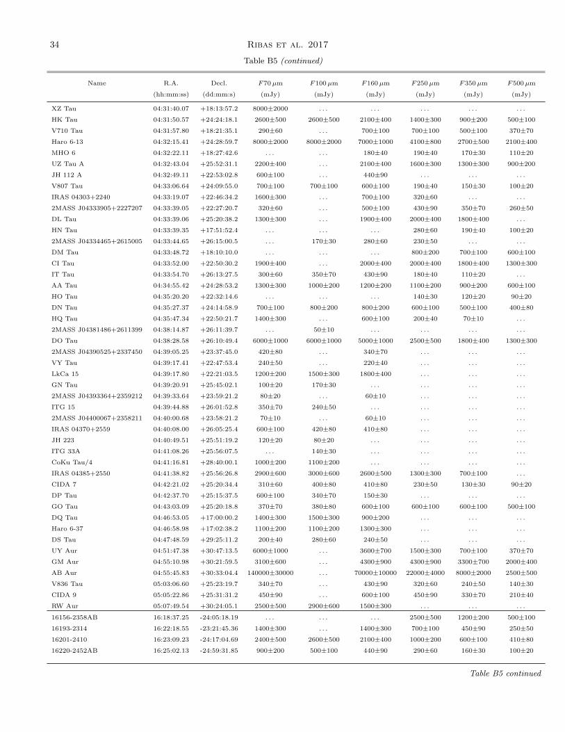
34 Ribas et al. 2017

Table B5 (continued)

Name R.A. Decl. F70µm F100µm F160µm F250µm F350µm F500µm

(hh:mm:ss) (dd:mm:s) (mJy) (mJy) (mJy) (mJy) (mJy) (mJy)

XZ Tau 04:31:40.07 +18:13:57.2 8000±2000 . . . . . . . . . . . . . . .

HK Tau 04:31:50.57 +24:24:18.1 2600±500 2600±500 2100±400 1400±300 900±200 500±100

V710 Tau 04:31:57.80 +18:21:35.1 290±60 . . . 700±100 700±100 500±100 370±70

Haro 6-13 04:32:15.41 +24:28:59.7 8000±2000 8000±2000 7000±1000 4100±800 2700±500 2100±400

MHO 6 04:32:22.11 +18:27:42.6 . . . . . . 180±40 190±40 170±30 110±20

UZ Tau A 04:32:43.04 +25:52:31.1 2200±400 . . . 2100±400 1600±300 1300±300 900±200

JH 112 A 04:32:49.11 +22:53:02.8 600±100 . . . 440±90 . . . . . . . . .

V807 Tau 04:33:06.64 +24:09:55.0 700±100 700±100 600±100 190±40 150±30 100±20

IRAS 04303+2240 04:33:19.07 +22:46:34.2 1600±300 . . . 700±100 320±60 . . . . . .

2MASS J04333905+2227207 04:33:39.05 +22:27:20.7 320±60 . . . 500±100 430±90 350±70 260±50

DL Tau 04:33:39.06 +25:20:38.2 1300±300 . . . 1900±400 2000±400 1800±400 . . .

HN Tau 04:33:39.35 +17:51:52.4 . . . . . . . . . 280±60 190±40 100±20

2MASS J04334465+2615005 04:33:44.65 +26:15:00.5 . . . 170±30 280±60 230±50 . . . . . .

DM Tau 04:33:48.72 +18:10:10.0 . . . . . . . . . 800±200 700±100 600±100

CI Tau 04:33:52.00 +22:50:30.2 1900±400 . . . 2000±400 2000±400 1800±400 1300±300

IT Tau 04:33:54.70 +26:13:27.5 300±60 350±70 430±90 180±40 110±20 . . .

AA Tau 04:34:55.42 +24:28:53.2 1300±300 1000±200 1200±200 1100±200 900±200 600±100

HO Tau 04:35:20.20 +22:32:14.6 . . . . . . . . . 140±30 120±20 90±20

DN Tau 04:35:27.37 +24:14:58.9 700±100 800±200 800±200 600±100 500±100 400±80

HQ Tau 04:35:47.34 +22:50:21.7 1400±300 . . . 600±100 200±40 70±10 . . .

2MASS J04381486+2611399 04:38:14.87 +26:11:39.7 . . . 50±10 . . . . . . . . . . . .

DO Tau 04:38:28.58 +26:10:49.4 6000±1000 6000±1000 5000±1000 2500±500 1800±400 1300±300

2MASS J04390525+2337450 04:39:05.25 +23:37:45.0 420±80 . . . 340±70 . . . . . . . . .

VY Tau 04:39:17.41 +22:47:53.4 240±50 . . . 220±40 . . . . . . . . .

LkCa 15 04:39:17.80 +22:21:03.5 1200±200 1500±300 1800±400 . . . . . . . . .

GN Tau 04:39:20.91 +25:45:02.1 100±20 170±30 . . . . . . . . . . . .

2MASS J04393364+2359212 04:39:33.64 +23:59:21.2 80±20 . . . 60±10 . . . . . . . . .

ITG 15 04:39:44.88 +26:01:52.8 350±70 240±50 . . . . . . . . . . . .

2MASS J04400067+2358211 04:40:00.68 +23:58:21.2 70±10 . . . 60±10 . . . . . . . . .

IRAS 04370+2559 04:40:08.00 +26:05:25.4 600±100 420±80 410±80 . . . . . . . . .

JH 223 04:40:49.51 +25:51:19.2 120±20 80±20 . . . . . . . . . . . .

ITG 33A 04:41:08.26 +25:56:07.5 . . . 140±30 . . . . . . . . . . . .

CoKu Tau/4 04:41:16.81 +28:40:00.1 1000±200 1100±200 . . . . . . . . . . . .

IRAS 04385+2550 04:41:38.82 +25:56:26.8 2900±600 3000±600 2600±500 1300±300 700±100 . . .

CIDA 7 04:42:21.02 +25:20:34.4 310±60 400±80 410±80 230±50 130±30 90±20

DP Tau 04:42:37.70 +25:15:37.5 600±100 340±70 150±30 . . . . . . . . .

GO Tau 04:43:03.09 +25:20:18.8 370±70 380±80 600±100 600±100 600±100 500±100

DQ Tau 04:46:53.05 +17:00:00.2 1400±300 1500±300 900±200 . . . . . . . . .

Haro 6-37 04:46:58.98 +17:02:38.2 1100±200 1100±200 1300±300 . . . . . . . . .

DS Tau 04:47:48.59 +29:25:11.2 200±40 280±60 240±50 . . . . . . . . .

UY Aur 04:51:47.38 +30:47:13.5 6000±1000 . . . 3600±700 1500±300 700±100 370±70

GM Aur 04:55:10.98 +30:21:59.5 3100±600 . . . 4300±900 4300±900 3300±700 2000±400

AB Aur 04:55:45.83 +30:33:04.4 140000±30000 . . . 70000±10000 22000±4000 8000±2000 2500±500

V836 Tau 05:03:06.60 +25:23:19.7 340±70 . . . 430±90 320±60 240±50 140±30

CIDA 9 05:05:22.86 +25:31:31.2 450±90 . . . 600±100 450±90 330±70 210±40

RW Aur 05:07:49.54 +30:24:05.1 2500±500 2900±600 1500±300 . . . . . . . . .

16156-2358AB 16:18:37.25 -24:05:18.19 . . . . . . . . . 2500±500 1200±200 500±100

16193-2314 16:22:18.55 -23:21:45.36 1400±300 . . . 1400±300 700±100 450±90 250±50

16201-2410 16:23:09.23 -24:17:04.69 2400±500 2600±500 2100±400 1000±200 600±100 410±80

16220-2452AB 16:25:02.13 -24:59:31.85 900±200 500±100 440±90 290±60 160±30 100±20

Table B5 continued

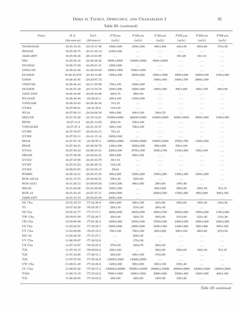
Disks in Taurus, Ophiuchus, and Chamaeleon I 35

Table B5 (continued)

Name R.A. Decl. F70µm F100µm F160µm F250µm F350µm F500µm

(hh:mm:ss) (dd:mm:s) (mJy) (mJy) (mJy) (mJy) (mJy) (mJy)

DOAR16AB 16:25:10.45 -23:19:11.96 1300±300 1000±200 900±200 420±80 280±60 170±30

IRS2AB 16:25:36.75 -24:15:42.12 2100±400 . . . . . . . . . . . . . . .

16225-2607 16:25:38.48 -26:13:53.99 . . . . . . . . . 90±20 60±10 . . .

SR4 16:25:56.18 -24:20:48.22 8000±2000 10000±2000 8000±2000 . . . . . . . . .

DOAR24 16:26:17.09 -24:20:21.41 1200±200 . . . . . . . . . . . . . . .

GSS31AB 16:26:23.38 -24:20:59.69 5000±1000 7000±1000 . . . . . . . . . . . .

DOAR25 16:26:23.678 -24:43:13.86 1800±400 3200±600 5000±1000 2800±600 2300±500 1500±300

GSS39 16:26:45.05 -24:23:07.72 . . . . . . 1900±400 3400±700 2600±500 . . .

VSS27AB 16:26:46.44 -24:11:59.99 700±100 1300±300 . . . . . . . . . . . .

DOAR28 16:26:47.49 -23:14:54.79 1000±200 1000±200 1000±200 800±200 600±100 400±80

16237-2349 16:26:48.66 -23:56:33.98 360±70 380±80 . . . . . . . . . . . .

WL18AB 16:26:48.99 -24:38:25.1 600±100 1400±300 . . . . . . . . . . . .

VSSG5AB 16:26:54.45 -24:26:20.56 70±10 . . . . . . . . . . . . . . .

GY204 16:27:06.61 -24:41:48.8 110±20 . . . . . . . . . . . . . . .

WL10 16:27:09.12 -24:34:08.29 900±200 600±100 340±70 . . . . . . . . .

SR21AB 16:27:10.28 -24:19:12.61 31000±6000 26000±5000 16000±3000 8000±2000 3900±800 1500±300

IRS36 16:27:15.9 -24:25:14.03 200±40 500±100 . . . . . . . . . . . .

VSSG25AB 16:27:27.4 -24:31:16.57 600±100 700±100 . . . . . . . . . . . .

GY289 16:27:32.67 -24:33:24.15 70±10 . . . . . . . . . . . . . . .

GY292 16:27:33.11 -24:41:15.14 2400±500 . . . . . . . . . . . . . . .

IRS48 16:27:37.18 -24:30:35.2 42000±8000 31000±6000 19000±4000 3700±700 1400±300 . . .

IRS49 16:27:38.31 -24:36:58.73 1400±300 1600±300 900±200 500±100 . . . . . .

GY314 16:27:39.43 -24:39:15.51 2300±500 2700±500 3300±700 1100±200 500±100 . . .

SR9AB 16:27:40.28 -24:22:04.31 900±200 600±100 . . . . . . . . . . . .

GY352 16:27:47.08 -24:45:34.79 60±10 . . . . . . . . . . . . . . .

GY397 16:27:55.24 -24:28:39.72 150±30 . . . . . . . . . . . . . . .

GY463 16:28:04.65 -24:34:56.15 39±8 . . . . . . . . . . . . . . .

WSB60 16:28:16.51 -24:36:57.95 900±200 1200±200 1000±200 1300±300 1000±200 . . .

ROX-42Cab 16:31:15.75 -24:34:02.21 220±40 320±60 . . . . . . . . . . . .

ROX-43A1 16:31:20.12 -24:30:05.03 1100±200 900±200 280±60 180±40 . . . . . .

IRS-60 16:31:30.88 -24:24:39.88 1200±200 . . . 800±200 390±80 230±50 70±10

ROX-44 16:31:33.45 -24:27:37.11 4300±900 . . . 2600±500 1500±300 900±200 500±100

16289-2457 16:31:54.74 -25:03:23.82 2000±400 . . . . . . . . . . . . . . .

SX Cha 10:55:59.73 -77:24:39.9 800±200 600±100 420±80 280±60 190±40 130±30

T5 10:57:42.20 -76:59:35.7 220±40 210±40 200±40 . . . . . . . . .

SZ Cha 10:58:16.77 -77:17:17.1 4000±800 3800±800 3600±700 2800±600 1900±400 1100±200

TW Cha 10:59:01.09 -77:22:40.7 420±80 340±70 400±80 310±60 210±40 110±20

CR Cha 10:59:06.99 -77:01:40.4 1600±300 2300±500 2700±500 2400±500 1800±400 1200±200

CS Cha 11:02:24.91 -77:33:35.7 3200±600 2900±600 2200±400 1400±300 900±200 500±100

CT Cha 11:04:09.09 -76:27:19.4 700±100 700±100 800±200 500±100 380±80 270±50

ISO 52 11:04:42.58 -77:41:57.1 . . . 200±40 . . . . . . . . . . . .

UY Cha 11:06:59.07 -77:18:53.6 . . . 170±30 . . . . . . . . . . . .

UZ Cha 11:07:12.07 -76:32:23.2 270±50 340±70 260±50 . . . . . . . . .

T25 11:07:19.15 -76:03:04.8 500±100 . . . 390±80 300±60 180±40 70±10

T28 11:07:43.66 -77:39:41.1 460±90 600±100 470±90 . . . . . . . . .

T29 11:07:57.93 -77:38:44.9 13000±3000 14000±3000 . . . . . . . . . . . .

VW Cha 11:08:01.49 -77:42:28.8 1400±300 900±200 600±100 220±40 . . . . . .

CU Cha 11:08:03.30 -77:39:17.4 120000±20000 70000±10000 60000±10000 39000±8000 24000±5000 12000±2000

T33A 11:08:15.10 -77:33:53.2 7000±1000 5000±1000 3900±800 2200±400 1300±300 600±100

T35 11:08:39.05 -77:16:04.2 400±80 320±60 160±30 120±20 . . . . . .

Table B5 continued

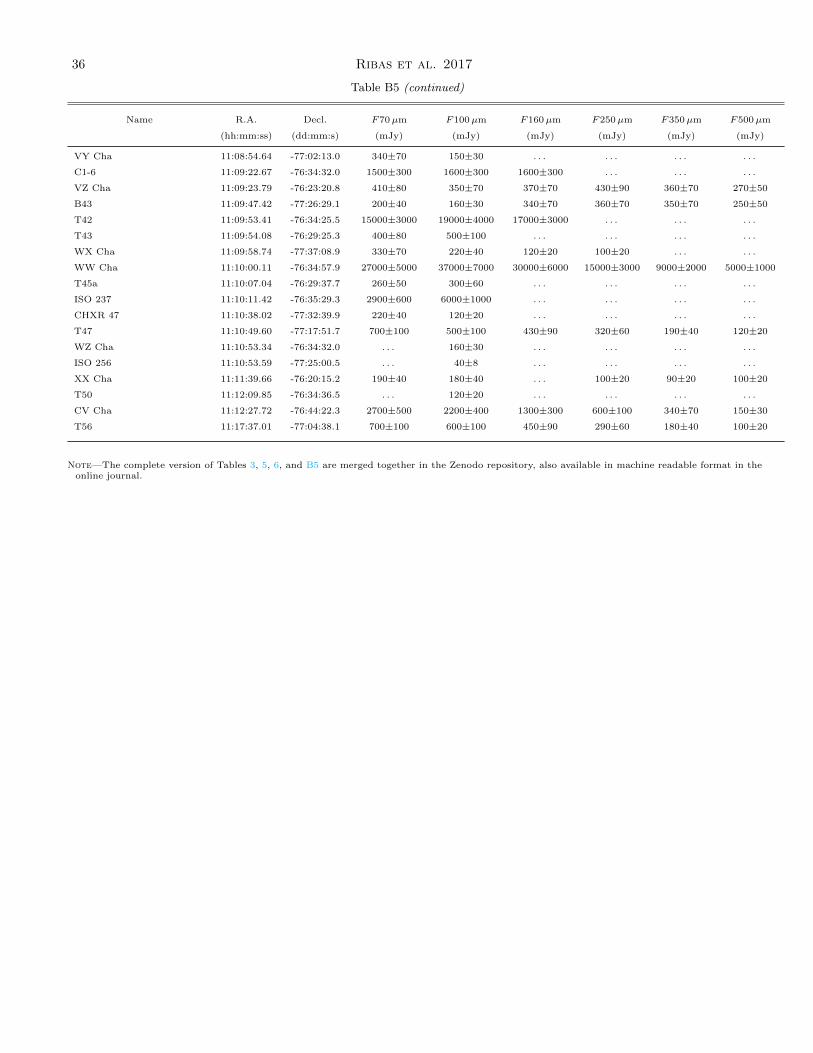
36 Ribas et al. 2017

Table B5 (continued)

Name R.A. Decl. F70µm F100µm F160µm F250µm F350µm F500µm

(hh:mm:ss) (dd:mm:s) (mJy) (mJy) (mJy) (mJy) (mJy) (mJy)

VY Cha 11:08:54.64 -77:02:13.0 340±70 150±30 . . . . . . . . . . . .

C1-6 11:09:22.67 -76:34:32.0 1500±300 1600±300 1600±300 . . . . . . . . .

VZ Cha 11:09:23.79 -76:23:20.8 410±80 350±70 370±70 430±90 360±70 270±50

B43 11:09:47.42 -77:26:29.1 200±40 160±30 340±70 360±70 350±70 250±50

T42 11:09:53.41 -76:34:25.5 15000±3000 19000±4000 17000±3000 . . . . . . . . .

T43 11:09:54.08 -76:29:25.3 400±80 500±100 . . . . . . . . . . . .

WX Cha 11:09:58.74 -77:37:08.9 330±70 220±40 120±20 100±20 . . . . . .

WW Cha 11:10:00.11 -76:34:57.9 27000±5000 37000±7000 30000±6000 15000±3000 9000±2000 5000±1000

T45a 11:10:07.04 -76:29:37.7 260±50 300±60 . . . . . . . . . . . .

ISO 237 11:10:11.42 -76:35:29.3 2900±600 6000±1000 . . . . . . . . . . . .

CHXR 47 11:10:38.02 -77:32:39.9 220±40 120±20 . . . . . . . . . . . .

T47 11:10:49.60 -77:17:51.7 700±100 500±100 430±90 320±60 190±40 120±20

WZ Cha 11:10:53.34 -76:34:32.0 . . . 160±30 . . . . . . . . . . . .

ISO 256 11:10:53.59 -77:25:00.5 . . . 40±8 . . . . . . . . . . . .

XX Cha 11:11:39.66 -76:20:15.2 190±40 180±40 . . . 100±20 90±20 100±20

T50 11:12:09.85 -76:34:36.5 . . . 120±20 . . . . . . . . . . . .

CV Cha 11:12:27.72 -76:44:22.3 2700±500 2200±400 1300±300 600±100 340±70 150±30

T56 11:17:37.01 -77:04:38.1 700±100 600±100 450±90 290±60 180±40 100±20

Note—The complete version of Tables 3, 5, 6, and B5 are merged together in the Zenodo repository, also available in machine readable format in theonline journal.

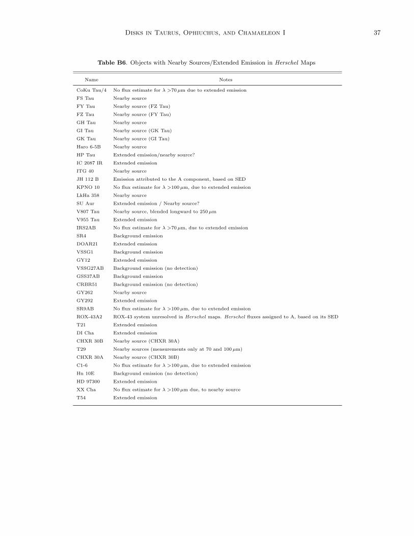
Disks in Taurus, Ophiuchus, and Chamaeleon I 37

Table B6. Objects with Nearby Sources/Extended Emission in Herschel Maps

Name Notes

CoKu Tau/4 No flux estimate for λ >70µm due to extended emission

FS Tau Nearby source

FY Tau Nearby source (FZ Tau)

FZ Tau Nearby source (FY Tau)

GH Tau Nearby source

GI Tau Nearby source (GK Tau)

GK Tau Nearby source (GI Tau)

Haro 6-5B Nearby source

HP Tau Extended emission/nearby source?

IC 2087 IR Extended emission

ITG 40 Nearby source

JH 112 B Emission attributed to the A component, based on SED

KPNO 10 No flux estimate for λ >100µm, due to extended emission

LkHa 358 Nearby source

SU Aur Extended emission / Nearby source?

V807 Tau Nearby source, blended longward to 250µm

V955 Tau Extended emission

IRS2AB No flux estimate for λ >70µm, due to extended emission

SR4 Background emission

DOAR21 Extended emission

VSSG1 Background emission

GY12 Extended emission

VSSG27AB Background emission (no detection)

GSS37AB Background emission

CRBR51 Background emission (no detection)

GY262 Nearby source

GY292 Extended emission

SR9AB No flux estimate for λ >100µm, due to extended emission

ROX-43A2 ROX-43 system unresolved in Herschel maps. Herschel fluxes assigned to A, based on its SED

T21 Extended emission

DI Cha Extended emission

CHXR 30B Nearby source (CHXR 30A)

T29 Nearby sources (measurements only at 70 and 100µm)

CHXR 30A Nearby source (CHXR 30B)

C1-6 No flux estimate for λ >100µm, due to extended emission

Hn 10E Background emission (no detection)

HD 97300 Extended emission

XX Cha No flux estimate for λ >100µm due, to nearby source

T54 Extended emission

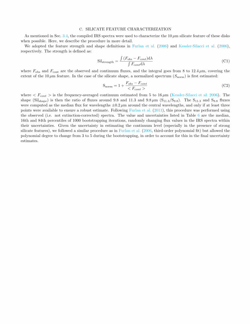
C. SILICATE FEATURE CHARACTERIZATION

As mentioned in Sec. 3.4, the compiled IRS spectra were used to characterize the 10µm silicate feature of these disks

when possible. Here, we describe the procedure in more detail.

We adopted the feature strength and shape definitions in Furlan et al. (2006) and Kessler-Silacci et al. (2006),

respectively. The strength is defined as:

Silstrength =

∫(Fobs − Fcont)dλ∫

Fcontdλ(C1)

where Fobs and Fcont are the observed and continuum fluxes, and the integral goes from 8 to 12.4µm, covering the

extent of the 10µm feature. In the case of the silicate shape, a normalized spectrum (Snorm) is first estimated:

Snorm = 1 +Fobs − Fcont< Fcont >

(C2)

where < Fcont > is the frequency-averaged continuum estimated from 5 to 16µm (Kessler-Silacci et al. 2006). The

shape (Silshape) is then the ratio of fluxes around 9.8 and 11.3 and 9.8µm (S11.3/S9.8). The S11.3 and S9.8 fluxes

were computed as the median flux for wavelengths ±0.2µm around the central wavelengths, and only if at least three

points were available to ensure a robust estimate. Following Furlan et al. (2011), this procedure was performed using

the observed (i.e. not extinction-corrected) spectra. The value and uncertainties listed in Table 6 are the median,

16th and 84th percentiles of 1000 bootstrapping iterations, randomly changing flux values in the IRS spectra within

their uncertainties. Given the uncertainty in estimating the continuum level (especially in the presence of strong

silicate features), we followed a similar procedure as in Furlan et al. (2006, third-order polynomial fit) but allowed the

polynomial degree to change from 3 to 5 during the bootstrapping, in order to account for this in the final uncertainty

estimates.