ATEX CLASS FILES, VOL. 14, NO. 8, AUGUST 2015 1 HSA-Net

1045-9219 (c) 2021 IEEE. Personal use is permitted, but republication/redistribution requires IEEE permission. See http://www.ieee.org/publications_standards/publications/rights/index.html for more information.

This article has been accepted for publication in a future issue of this journal, but has not been fully edited. Content may change prior to final publication. Citation information: DOI 10.1109/TPDS.2021.3111810, IEEETransactions on Parallel and Distributed Systems

JOURNAL OF LATEX CLASS FILES, VOL. 14, NO. 8, AUGUST 2015 1

HSA-Net: Hidden-State-Aware Networks forHigh-Precision QoS PredictionZiliang Wang, Xiaohong Zhang, Meng Yan, Ling Xu and Dan Yang

Abstract—The high-precision QoS (quality of service) prediction is based on the comprehensive perception of state information ofusers and services. However, the current QoS prediction approaches have limited accuracy, for most state information of users andservices (i.e. network speed, latency, network type, and more) are hidden due to privacy protection. Therefore, this paper proposes ahidden-state-aware network (HSA-Net) that includes three steps called hidden state initialization, hidden state perception, and QoSprediction. A hidden state initialization approach is developed first based on the latent dirichlet allocation (LDA). After that, ahidden-state perception approach is proposed to abstract the initialized hidden state by fusing the known information (e.g. service IDand user location). The perception approach consists of four hidden-state perception (HSP) modes (i.e. known mode, object mode,hybrid mode and overall mode) implemented to generate explainable and fused features through four adaptive convolutional kernels.Finally, the relationship between the fused features and the QoS is discovered through a fully connected network to complete thehigh-precision QoS prediction process. The proposed HSA-Net is evaluated on two real-world datasets. According to the results, theHSA-Net’s mean absolute error (MAE) index reduced by 3.67% and 28.84%, whereas the root mean squared error (RMSE) indexdecreased by 3.07% and 7.14% compared with ten baselines on average in the two datasets.

Index Terms—Service recommendation, Convolutional neural network, QoS prediction, Hidden states, Feature fusion.

F

1 INTRODUCTION

W ITH the growing number of Web services, it is es-sential to determine how to recommend high-quality

services to users. The main idea of service recommendationis to automatically predict the QoS values of the Web ser-vices that the user does not invoke and then recommendthe most suitable Web services to the user through thesepredicted QoS values. Therefore, QoS prediction is a keystep in service recommendation. QoS (e.g. response timeand throughput) [1] [2] is considered to be an importantcriterion for evaluating the quality of Web services [3] [4]. Infact, reliable QoS data can effectively recommend optimalservices to potential users. A recommended low-quality ser-vice (e.g., no response for a long time) may result in the lossof potential users. For example, service 0-5 is a public serviceused by a large number of users. The predicted responsetimes between user 0 and five services were reported 5.982,2.13, 0.854, 0.693, 0.866, and 1.833 seconds. We will givepriority to recommend high-quality services 3 and 4 to theuser 0. Therefore, it is important to predict the unknown

• This work was supported in part by the National Key Research and De-velopment Project of China (No. 2018YFB2101200), Special Funds for theCentral Government to Guide Local Scientific and Technological Develop-ment (No. YDZX20195000004725), National Natural Science Founda-tion of China (No. 61772093), the Key Project of Technology Innovationand Application Development of Chongqing under (No. cstc2019jscx-mbdxX0020), the Chongqing Science and Technology Plan Projects (No.cstc2018jszx-cyztzxX0037), and the Chongqing Technology Innovationand Application Development Project (No. cstc2019jszx- mbdxX0064).

• Ziliang Wang, Xiaohong Zhang, Meng Yan, Ling Xu, Dan Yang arewith Key Laboratory of Dependable Service Computing in Cyber PhysicalSociety (Chongqing University), Ministry of Education, China and Schoolof Big Data and Software Engineering, Chongqing University, Chongqing401331, China.

• Xiaohong Zhang and Meng Yan are the corresponding authors. E-mail:xhongz,[email protected]

QoS data based on historical data. This area has attracted agreat deal of research interest [5] [6] [7].

Many challenges limit the accuracy of QoS prediction.For example, data sparsity is a major challenge in QoSprediction. Although there is a large number of services,users have access to a limited number of services whichmakes the user-service matrix sparse. According to theresearch literature, a common approach to the reliable QoSprediction is collaborative filtering (CF) [8] [9] [10]. In fact,CF is mainly based on similarity calculation performedby similar users and similar services to predict unknownQoS values. Due to the simplicity and availability of CF,it is considered a widely used QoS prediction approach.However, the sparsity and imbalance of QoS data makeCF suffer from the limited prediction accuracy and weakscalability [11].

To overcome CF limitations, researchers proposed inte-grating deep learning approaches with the CF technology toimprove the QoS prediction accuracy [12] [13] [14]. Amongthe existing approaches based on deep learning, obtainingas much information as possible is still the core idea foraccuracy improvement. For example, Zhang et al. used loca-tion information as features and considered the user–servicedistance correlation to realize the QoS prediction [14]. Thedeep learning technology improves the prediction accuracyto a certain extent but requires effective information knownas prediction conditions, such as location and temporalinformation. According to the previous studies, the QoS isoften closely related to a user’s state of the user and serviceitself when the service is used [15] [16]. For example, auser’s network speed and the service load rate will directlyaffect the QoS [17]. Compared with algorithms that do notconsider known information, the models that consider moreinformation can lead to more accurate QoS predictions.

Authorized licensed use limited to: CHONGQING UNIVERSITY. Downloaded on September 13,2021 at 07:03:33 UTC from IEEE Xplore. Restrictions apply.




For example, Chen et al. [18] further improve improvedthe accuracy of prediction through an extended version ofthe approach proposed by Wu et al.. [19] to embed theservice location and the user location information in vectors.However, most current methods benefit from only the exist-ing information and rarely consider the latent relationshipbetween different information. In summary, there are stilltwo challenges to the high-precision QoS prediction:

1) Limited information: The known information is lim-ited, for it is difficult to collect much state informa-tion on services and users due to cost and privacyissues.

2) Independent features: Most studies use the knowninformation on the QoS as independent features. Infact, just a few studies analyzed how to determinethe relationship between different information onthe QoS.

To tackle the above challenges, this paper proposes ahidden-state-aware networks (HSA-Net), which is mainlybased on the idea of initializing the hidden-state informationon users and services in the first step. As a result, it ispossible to overcome the challenge of limited information.In the second step, the information is divided into fourcategories, i.e. known user information, hidden-state infor-mation of users, known service information, and hidden-state information of services. The perception approach isthen proposed. It includes four hidden-state perception(HSP) modes to obtain the fused features by abstractingand fusing different information. Each HSP mode achievesa comprehensive perception of information based on differ-ent classifications through an adaptive convolution kernel.This approach can overcome the challenge of independentfeatures and enhance the compatibility to different datasets.In the third step, fully connected networks are employed tolearn the relationship between the fused features and theQoS in order to achieve the high-precision QoS prediction.

In summary, the main contributions of this paper are asfollows:

a) We proposed a novel approach based on HiddenState Aware Network (HSA-Net) with three steps,i.e., hidden state initialization, hidden state percep-tion, and QoS prediction. HSA-Net provided a noveland effective solution for addressing the data incom-pleteness problem in the field of QoS prediction.

b) A hidden-state perception approach is also proposed.It includes four HSP modes (i.e. known mode, objectmode, hybrid mode, and overall mode) based ondifferent convolutional kernels. Such modes encodethe information of a specific category to obtain fusedfeatures (i.e. known features, object features, hybridfeatures, and overall features) where the convolu-tional adaptive kernels are adjusted dramatically ac-cording to the amount of features.

c) A few large-scale experiments are conducted to eval-uate the effectiveness of the proposed HSA-Net bycomparison with ten state-of-the-art baselines on tworeal-world datasets. According to the experimental

results, the HSA-Net outperforms all the baselines interms of the QoS prediction precision 1.

The remainder of this paper is organized as follows.In Section 2, related work is described. Section 3 providesthe description of the proposed HSA-Net. Section 4 dis-cusses the study set includes datasets, evaluation criteria,and more. Section 5 presents the experimental results andanalysis in detail. The last section, concludes the paper andintroduces the direction of future work.

2 RELATED WORK

To predict QoS, two review studies have recently beenpresented in [20] and [21]. Roughly speaking, the QoSprediction approaches can be classified into two categories:collaborative filtering-based QoS prediction approaches anddeep learning-based QoS prediction approaches.

2.1 Collaborative Filtering-Based QoS Prediction Ap-proaches

In this approach, a User-Service QoS matrix is the basicdata source. This paper uses the User-Service QoS matrixdefinition that is similar in most studies [22], [23], [24],[25], [26], [27], [28]. CF-based Qos prediction approaches canbe divided into two categories: memory-based and model-based. Memory-based approaches consider response time,throughput, or location as a similarity measure betweenusers or services. The approach includes user-based [29],service-based [30], and a combination of the user and service[31]. The key step is to perform similarity calculations onusers or services. For example, Zheng et al. introduced aQoS prediction approach with a similarity computation ap-proach of similar neighbors [32]. Model-based approaches,on the other hand, apply techniques like matrix factorization(MF). This is an effective technique to implement recom-mender systems [33] [34] [35] [36], which has been exten-sively utilized to implement the QoS predictors in recentyears. Ren et al. proposed a support vector machine-basedCF approach to found the services that be truly preferred bya user [37]. The advantage of the QoS prediction approachbased on collaborative filtering is that little data is required,but due to the lack of information and data sparsity, satisfac-tory prediction accuracy is often not achieved by a relatedapproach.

To further improve the accuracy of collaborative filter-ing, many researchers have begun to focus on additionalinformation (such as time and locations). For example,Chen et al. considered the user’s trust degree and locationinformation for QoS prediction [38]. Tang et al. and Liu etal. used the locations of users and services to improve theaccuracy of QoS prediction effectively [39] [40]. Among var-ious models with additional information, latent factors (LF)-based QoS predictors are prevalent due to their scalabilityand high prediction accuracy [41] [42] [43] [44] [45]. Luo et al.proposed a highly accurate prediction approach for missingQoS data by ensembling nonnegative latent factor (NLF)models [46]. Wu et al. propose a posterior-neighborhood-regularized latent factors (PLF) model for highly accurate

1. Our replication package:https://github.com/HotFrom/HSA-Net





QoS prediction [47]. The main idea of the latent factor (LF)-based approach is to improve the accuracy of prediction bydiscovering the hidden state of users and services. Simi-larly, Luo proposed a latent ability model (LAM) that caninitialize the hidden capabilities of employees and services[48] but lacks an effective prediction approach. Althoughthe additional information contributes to the accuracy ofthe CF method, the prediction accuracy still does not reachthe expected because it can only learn the linear and low-dimensional relationship.

The hidden state initialization step is closely related tothe latent factor-based approaches because it also considersthe hidden information of user and service [15]. Comparedwith the MF-based approaches that only obtain a singleuser latent matrix and service latent matrix, the proposedinitialization approach in this paper can set any numberof hidden states. By doing this, HSA-Net can use moreinformation to provide accurate predictions.

2.2 Deep Learning-Based QoS Prediction ApproachesIn recent years, deep neural networks have emerged

as an effective approach to recommended services. Thisapproach, which our approach belongs to, captures the non-linear relationship by considering the hidden state infor-mation of the object. He et al. are the first researchers whoapplied deep learning techniques in the recommended field[12]. Moreover, Kim et al. proposed the ConvMF modelfor QoS prediction that integrates the convolutional neuralnetwork (CNN) into probabilistic matrix factorization (PMF)to captures known information [49]. Similarly, deep learningapproaches that use the timeslices information are alsowidely used in QoS prediction tasks. For example, Xionget al. proposed a novel personalized LSTM based matrixfactorization approach that can seize the dynamic latentrepresentations of users and services and can be seasonablyupdated to deal with the new data [50].

Deep learning improves the accuracy of prediction tosome extent but requires a lot of additional effective infor-mation as prediction conditions [51], [52], [53], [54], [55]. Tofurther mining hidden information, Xiong et al. proposeda deep hybrid collaborative filtering approach for servicerecommendation that can find the complex invocation rela-tions between mashups and services by using a multilayerperceptron [56]. HSA-Net is inspired by other domains ofthe research base on deep learning methods using knowninformation for QoS prediction [57]. The main difference be-tween the HSA-Net and those methods is that HSA-Net usesmore hidden information and further captures the latentrelationship between different information rather than onlythe relationship between independent features and QoS.Consequently, the HSA-Net can mitigate the challenges ofindependent features for QoS prediction.

3 PROPOSED APPROACHThe architecture of HSA-Net is shown in Figure 1, which

includes three steps: hidden state initialization, hidden stateperception, and QoS prediction:

Hidden State Initialization: An LDA-based hidden stateinitialization algorithm to initialize M hidden states of usersand services: (p1...pm) and (q1...qm).

Hidden State Perception: The hidden state percep-tion step includes four different HSP modes to capturethe impact of different information. We abstract and fuse(p1...pm), (q1...qm) and known information of users andservices (Ku1 ...Kuo , Ks1 ...Kso ) through different convolu-tion operations to obtain four fusion features. Furthermorethe size of the convolution kernel of each HSP mode canbe automatically adapted according to the number of theknown information (O) from the dataset and the number ofhidden information (M).

QoS Prediction: The QoS prediction step captures therelationship between the four fusion features of the secondstep and QoS through a fully connected neural network toachieve high-precision QoS prediction.

3.1 Hidden State InitializationSince the original information from the QoS dataset

contains little information, we use a hidden state initial-ization algorithm to initialize M hidden states of user andM hidden states of service closely related to response time.The response time is a complex variable that is affected byvarious factors of the user and the service itself. In mostcases, we cannot access sufficient information such as usernetwork speed and service load to predict response time;hence response time is modeled as a mixture of hidden stateinformation and known information.

Figure 2 describes how the hidden state variables inter-act with the observation variables to learn the distribution ofthe hidden state. We provided the definition of notations inTable 1 and the hidden state initialization steps in Algorithm1.

3.1.1 Parameter definitionIn this section, four probability distributions are first

defined and how to calculate them is then discussed.Definition 1: Let L = 〈U, S, T 〉 denote the QoS records

of the form (ui,si,ti), ui ∈ U , si ∈ S, ti ∈ T , 1 ≤i ≤ n. U is the user identifier. S is the service identifier,and T is the response time for user U to access serviceS. Let parameter M denote the number of hidden statetype. The set Pi={pk(1 ≤ k ≤M, 1 ≤ i ≤ nu)} contains mhidden state that are contained by the user i. The setQi={qk(1 ≤ k ≤M, 1 ≤ i ≤ ns)} contains M hidden statethat are contained by the service i. n, nu, ns are the numberof records, the number of users and the number of services,respectively.

The matrix βu ={βu{i,j}

}is used to denote the prob-

ability for assigning all M hidden states to all nu users(1 ≤ i ≤M, 1 ≤ j ≤ nu) and the matrix βs =

{βs{i,j}

}denotes the probability for assigning all M hidden statesto all ns services. We initialize βu and βs with the standardnormal distribution.

Definition 2: The Θs is the frequency of various hiddenstate assignments on services. Θs{i} is the fraction of distinctservices contains hidden state i, satisfying Σmi=1Θs{i} = 1.Dirichlet Prior is the smoothing distribution function toguarantee that the element of the hidden state would notbe too small or too big. The Θs was defined the priordistribution that its probability density function by Dirichletprior:

Θs ∼ Dirichlet(),Θsi = 1/M, 1 ≤ i ≤ ns (1)





Fig. 1: The framework of HSA-Net. Step I: HSA-Net initializes M hidden states information of users and M hidden statesinformation of services. Then 2×M hidden state information and 2×O known information are encoded into V-dimensional

vector by Ont-hot. Step II: Four HSP modes generate four interpretable fusion features through four different convolutionoperations. Step III: HSA-Net uses a three-layer fully connected network to achieve high-precision QoS prediction.

Similarly, we define Θu by using the same Dirichlet Priorwith the same prior distribution:

Θu ∼ Dirichlet(),Θui= 1/M, 1 ≤ i ≤ nu (2)

We consider the following sampling process: the hiddenstate is a sample from the state set of size m, accordingto the frequency Θu. The probability of the hidden statescontained by ui is exactly Zu. Formally:

Zu|Θu ∼ Discrete(Θu) (3)

Similarly, the probability of the hidden state contained by siis exactly Zs. Formally:

Zs|Θs ∼ Discrete(Θs) (4)

Definition 3: For each record, we consider the probabil-ity of assigning hidden state Zu to the user Ui as well as thefactors Zs to the service Sj . The probability βu is defined asthe parameter for modeling the relation between the hiddenstate Zu and ui. We have:

ui|Zu, βu ∼ Discrete(βu{Zu}) (5)

In a similar fashion, we have:

si|Zs, βs ∼ Discrete(βs{Zs}) (6)

as show in Figure 2, βu and βs have size nu × M andns ×M , respectively.

Definition 4: The Cu is the complexity factor of theuser representing user’s sophistication factor on responsetime. It is a vector of size nu. In this case, it represents thecomplexity factor of all users and initialized to Cui = 10,1 ≤ i ≤ nu. Identically, Cs is the complexity factor of servicerepresents the service’s sophistication factor on responsetime. It represents the complexity factor of all services and

TABLE 1: Notations and Descriptions

Notations Descriptions

O The number of known information.M The number of hidden states.Ns The number of services.Nu The number of users.N Number of records.Θs Θs{i} denotes the probability of existence

hidden state i for all services.Θu Θu{i} denotes the probability of existence

hidden state i for all users.βs βs{i} denotes the distribution of hidden

states owned by service i, βs{i,j} denotes theservice i’s hidden state j.

βu βu{i} denotes the distribution of hiddenstates owned by user i, βu{i,j} denotes theuser i’s hidden state j.

initialized to Csj = 10, 1 ≤ i ≤ ns.

3.1.2 Response time samplingThe most important step is sampling response time ti

given the i QoS record (ui, si, ti). ti as the object of observa-tion is affected by different factors of users and services. Foreach record, the conditional probability is used to representits distribution:

ti|Zu, Zs, Cu, Cs, w ∼ Φ(ti;λi,j,k) (7)

where function Φ is exponential distribution with parameterλ regarding response time:

Φ(ti, λi,j,k) = λi,j,ke(−ti∗λi,j,k) (8)





Fig. 2: The graphical model of hidden state initialization step. Θu is the hidden state probability distribution for all users. βu isthe hidden state probability distribution of each user. Θs is the hidden state probability distribution for all services. βs is the

hidden state probability distribution of each service.

where

λ−1i,j,k =

{CujCsk if ti < η

CujCskw else(9)

where j denotes the service and k denotes the user in theith record. w is a penalty coefficient, the initial value is 50.The range of response time is 0-20 second. According tothe exponential distribution in Eq. 8, the records with lowerresponse times will get higher feedback. When the responsetime is close to 0 second, the feedback value is close to 1, andwhen the response time is close to 20 second, the feedbackvalue is smaller. The significance of the penalty coefficient isto increase the score gap between the record with a responsetime of 5-20 second and the record with a response time of 0-5 second. According to the exponential distribution, a recordof 5-20 will get a lower score. Because in the QoS predictionproblem, we hope to successfully predict records with a too-long response time, which will reduce the recommendationof these services to users. The initial value of the complexcoefficient does not have any meaning, and the purpose is togive an initial gradient to the gradient descent algorithm. ηisa constant. When the response time is less than η seconds,the penalty does not be imposed.3.1.3 Parameter estimation

The Γ(Θu,Θs, βu, βs, w, Cu, Cs) is a set of parametersin our hidden states initialization algorithm, which mustbe learned. In this place, we choose maximum a posteriori(MAP) to complete parameter estimation. In this step, weuse the initialization values of the parameters as the priordistribution and use the QoS record Q as the observation ob-ject to obtain the posterior distribution P (Γ|Q). The specificcalculation approach is as follows:

P (Γ|Q) = Zn∏i=1

m∑j=1

m∑k=1

τi,j,kΦ(sij ;λi,j,k) (10)

where

τi,j,k = βu{j,ui}βs{j,si}Θu{j}Θs{k}1

B(M)

m∏i=1

(Θs{i}Θs{i})M−1

(11)Z is a constant and keeps the sum of all probabilities

equal to 1. In the above announcement, ui and si rep-

resent the service number of the user recorded in thei-th. To solve this MAP problem, the EM (expectation-maximization) algorithm is used to update the set of param-eters {Θu,Θs, βu, βs}, and the set {Cu, Cs, w} are updatedwith the gradient descent (GD) algorithm at the same time.In the case that the objective function and the data aredetermined, the solution space is also determined. Differentinitial settings may have different initial gradients, but theywill produce the same final value.

In Algorithm 1, E-step refers to the expectation step. Wecalculate the probability of hidden states by Bayes theorem:

F ti,j,k = P (ui, tk|ui, si, ti,Γ)

= τi,j,kΦ(sij ;λi,j,k)(12)

M-step refers to the maximization step. We update parame-ters Γ by maximizing the condition expectation.

T (Γ|Γt) =

n∑i=1

m∑j=1

m∑k=1

F ti,j,klogP (Γ|Q)

=

n∑i=1

m∑j=1

m∑k=1

F ti,j,klog(τi,j,kΦ(sij ;λi,j,k))

(13)

Then we have:

Θt+1s = argΘu

maxT (Γ|Γt)

= argΘumaxn∑i=1

m∑j=1

m∑k=1

T (logΘs{j}+

(m− 1)m∑i=1

log(Θs{i}))

=(m− 1)n+

∑ni′=1

∑mk=1 F

ti′ ,i,k

(m(m− 1) + 1)n

(14)

andβt+1uj,p

=argβumaxT (Γ|Γt)

=

n∑i=1

m∑k=1

F ti,j,kI(ui = p)(15)





Algorithm 1 Hidden state initialization algorithm

Input: Q: (ui,si,ti) variables: nu is the number of users, nsis the number of services. m is the number of hiddenstate and n is the number of records.

Output: (βu, βs)

//E-STEP1: while Lt+1/Lt > γ do2: for i = 1 to n do3: for j = 1 to m do4: for k = 1 to m do5: F ti,j,k = τi,j,kΦ(sij ;λi,j,k)6: end for7: end for8: end for

//M-STEP9: for i = 1 to m do

10: Θt+1u =

(m−1)n+∑n

i′=1

∑mk=1 F

t

i′,i,k

(m(m−1)+1)n

11: Θt+1s =

(m−1)n+∑n

i′=1

∑mj=1 F

t

i′,j,i

(m(m−1)+1)n12: for q = 1 to nu do13: βt+1

u{i,q} =∑ni′=1

∑mk=1 F

ti′ ,i,k

I(ui = q)14: end for15: for q = 1 to ns do16: βt+1

s{i,q} =∑ni′=1

∑mj=1 F

ti′ ,j,i

I(si = q)17: end for18: end for

//GD-STEP19: for q = 1 to nu do20: Ct+1

ui= Ctui

+ % ∗ ∂P (Γ|Q)t

∂Ctui

21: end for22: for q = 1 to ns do23: Ct+1

si = Ctsi + % ∗ ∂P (Γ|Q)t

∂Ctsi

24: end for25: wt+1 = wt + % ∗ ∂P (Γ|Q)t

∂wt

26: Lt+1 = P (Γ|Q)27: end while

return (βu, βs)

βt+1sk,q

=argβsmaxT (Γ|Γt)

=n∑i=1

m∑j=1

F ti,j,kI(si = q)(16)

I(si = q) means that when si = q, the return value is 1,otherwise the value is 0. We supplement the steps of the GDalgorithm in detail to update the parameters (Cu, Cs, w):

∂P (Γ|Q)t

∂Ctsi

=

n∑i=1

m∑j=1

m∑k=1

F ti,j,k(− 1

Cuq

+ti

Cu(ui)C2

sq

(I(j = k) +1

wI(j 6= k))))I(ui = q)

(17)for Cs:

∂P (Γ|Q)t

∂Ctsi

=

n∑i=1

m∑j=1

m∑k=1

F ti,j,k(− 1

Csq

+ti

Cs(si)C2

uq

(I(j = k) +1

wI(j 6= k))))I(si = q)

(18)

and the gradient for w:

∂P (Γ|Q)t

∂w=

n∑i=1

m∑j=1

m∑k=1

F ti,j,k(− 1

w+

tiCu(ui)

Cs(si)w

)I(j 6= q)

(19)

The γ is a constant less than 0.01, which is used as theconvergence condition of the algorithm. In algotithm1, line1 and line 26 provides a way to calculate the terminationcondition. Finally, we use the results returned by Algorithm1 as the hidden state of users and services.

3.2 Hidden State Perception

3.2.1 Input layer

To train the neural network, we input the user knowninformation Kui

, user’s hidden states Pi, service knowninformation Ksj , and service’s hidden states Qj into theembedding layer of Keras, which can be regarded as afully connected layer without bias term. The latent stateinitialization algorithm calculates the latent state of usersand services, which is a floating-point value. To implementthe embedding layer operation in the neural network, weexpand each state value by 100 times and de-integer. Inthe sense of solely, each information goes through one-hotencoding that makes the feature to 1xV dimension vector sothat the ith position is 1 and the other is 0. The mathematicalexpression of this step is as follows:

Kvui

= f1(TT1 ui + b1) (20)

P vi = f1(TT1 pi+ b2) (21)

Kvsj = f1(HT

1 sj + b3) (22)

Qvj = f1(HT1 qj + b4) (23)

where T1 and H1 stand for the users and service’s embed-ding weight matrix, respectively. For better feature com-bination, we combine the user known information vectorwith the user hidden state information vector to obtain theuser feature vector. Similarly, we can get the service featurevector. Then, we concatenate them to get the input vector.The simplified step is as follows:

Input = Φ(Kui , pi,Ksj , qj , U, S, axis = 1) (24)

where Φ is a mergence operation by Keras, and axis=1indicates that the operation is performed line by line.

3.2.2 HSP modes

We designed four HSP modes by considering the mean-ing of hidden information in different situations throughreal experience. In the section, we described the settingand meaning of HSP modes in detail. We divide all QoSinformation into four categories: user known information(Ku1 ...Kuo ), service known information (Ks1 ...Kso ), userhidden states information (p1...pm), and service hiddenstates information (q1...qm). To select a more reasonablecombination of features according to the degree of contri-bution to the predicted response time, different convolutionkernels have been used to calculate the impact betweendifferent information to generate specific fused features.





The hidden state perception step in the network can beexpressed as:

Fm = Φ(f1, f2, f3, f4) (25)

Fm is the output of HSP modes, f1, f2, f3 and f4 are thefused features obtained after convolution operation withdifferent settings, which are described as follows:

fi = wi ∗ F + bi (26)

Figure 2 shows the HSP mode proposed in this paper.The following details the meaning and output of each HSPmode:

The hybrid mode solves a defect of the hidden state ini-tialization algorithm: the user and the service initialize thesame number of hidden states. However, service providerstend to have more stable networks, and their hidden statesmay not be as large as users. It is necessary to consider therelationship between the different number of hidden statesof the service and other states.

Hybrid Mode: The convolution kernel of hybrid modeis 1.5 ∗ (M +N)× 1 and the strides = 0. Each convolutionoperation of hybrid mode is focused on different K userfeatures and J service features. At the same time, K isdecreasing and J is increasing during each convolution.0.5 ∗ (M +O) < K < M +O , 0.5 ∗ (M +O) < j < M +O,j + k = 1.5 ∗ (M +O).

Hybrid Features: The hybrid mode produces 0.5 ∗ (M +N) + 1 hybrid features. Each hybrid feature focuses ondifferent user features and service features. The reason forthis is that the quality of service may be affected by differentamounts of service information or user information ratherthan the same amount of users and service information. Theeffect of hybrid features is to explore the impact of fusedfeatures from different numbers of service features anduser features on service quality, respectively. For example,the interaction between all user information and a smallamount of service information is considered in the firsthybrid feature.

The object mode considers the states of users or servicesalone by generating object features. We can focus on thestate of the object itself to judge the quality of service. Thisis because there are services and users with poor states. InFigure 3, the response time of many users to call certainservices is about 12s, which is caused by the poor states ofthe objects of these services.

Object Mode: The convolution kernel of object modeis (M + O) × 1 and the strides = (M + O) − 1. Theobject mode performs twice convolution operations. Thefirst convolution operation fuses all user features (Ku1:o

andp1:m) to obtain user object features. The second convolutionoperation fuse all service features (Ks1:o and q1:m) to obtainthe service object feature.

Objects Features: The object mode produces two differentobject features: user object features and service object fea-tures. The effect of object feature is to explore the impact ofuser and service information on service quality respectively.For example, if user x cannot access a certain service dueto network states, the states of his state features will have adecisive effect on QoS prediction.

In QoS prediction, the known information is locationinformation, and this module will play a role similar to the

distance module in other studies.Known Mode: The convolution kernel of known mode

is O × 1 and the strides = (M + O) − 1. The knownmode performs twice convolution operations. The first con-volution operation fuses all user known features (Kuo

) toobtain user known fused features. The second convolutionoperation fuse all the service known features (Kso ) to obtainthe service known fused feature.

Known Features: The known mode produces two differentknown features: users known features and services knownfeatures. Light blue indicates that the known features ofthe user. Orange indicates the known fused features of theservice. The effect of known features is to explore the impactof known information on service quality respectively. Forexample, the known features in the dataset D2 may be easierto pay attention to the latent relationship (distance) becausethe known information of D2 is location information.

The overall model calculates the standard value throughall the features. The standard value can also be directlyregarded as the performance of the final feature—responsetime. We will use other fusion features that from the threeHSP modes to calibrate this value further. Overall Mode:The convolution kernel of overall mode is 2 ∗ (M + O)and the strides = 0. The overall mode performs onceconvolution operations. This convolution operation fuses allinformation to obtain the overall fused feature.

Overall Features: Green represents the overall fused fea-ture of all information. The overall fused feature focuses onthe impact of all information on service quality.

M is the number of hidden states. O is the number ofknown information of the user or service given by the sourcedataset. When O = 1, the known information includesidentification(ID). The known information includes ID, loca-tion information, and autonomous system (AS) informationwhen O = 3.

3.3 QoS PredictionIn this step, a fully connected neural network is used

to achieve high-precision QoS prediction. The network isused to process the input vector from the hidden stateperception step for learning the high-dimensional nonlinearrelationship and complete the QoS prediction. First of all,we reshape the dimensions of the fused feature through theflatten layer of Keras to meet the input required of the fullyconnected layer. Secondly, we use the Batch Normalizing(Bn) layer to prevent overfitting. Bn layer can also speed upnetwork training and prevent the gradient from disappear-ing. Finally, we chose ReLu as the activation function for thefirst two layers because it can speed up the convergence ofthe model. To get an accurate prediction value, we chose the”Linear” function as the activation function of the last layer.The prediction step is defined as follows:

FC2∗V = f3(WT3 x+ b3) (27)

FCV = f2(WT2 x+ b2) (28)

Qu,s = FC1 = f1(WT1 x+ b1) (29)

where Qu,s is the predictive QoS value that user i useservice j. V is the number of neurons. The FCv means that vneurons are set in this layer. Wd is the corresponding weightmatrix and bd is the bias term of the d-th layer.





3.3.1 Loss function

We can roughly classify the mainstream loss functionsinto two types: loss functions for regression problems andloss functions for classification problems. QoS predictionproblem is a regression problem. The commonly used lossfunctions for the regression problem are mean square errorfunction (MSE), mean absolute error function (MAE), andHuber function. In this paper, after a detailed comparisonexperiment, we chose the MAE function as the loss function,which is defined as follows:

Loss =1

n

n∑i=1

|yi − yi|abs (30)

In Section 4, we discuss in detail the reasons for choosingMAE function.

3.3.2 Complexity analysis

In this section, we analyze the time complexity of theproposed HSA-Net.

In algorithm 1, the time complexity of lines 2-8 isO(n × m × m), where n represents the number of recordsand m is the number of hidden states(m � n). The timecomplexity of lines 9-11 is O(1) because m is a constant. Thetime complexity of lines 12-17 is O(m × nu) +O(m × ns),where nu and ns represent the number of users and services,respectively. The time complexity of lines 19-26 is O(1).Therefore, the time complexity of the step (lines 2–26) isO(n×K). Then the complexity of algorithm 1 is given by

T = O(n×m×m+ 1 +m× nu +m× ns + 1)

≈ Θ(K × n)(31)

In the HSP modes, the time complexity of Eq.(20) -Eq.(26) is O(n). Then we perform a total of four one-dimensional convolution operations. Therefore, the timecomplexity of the forward propagation process is O(n×k×4) in Eq.(28).

In the QoS prediction step, the time complexity of Eq.(32)is O(n×k). The time complexity of Eq.(29) - Eq.(31) is O(n×k) because the time complexity of the forward propagationis the same as the backpropagation.

Overall, the time complexity of HSA-Net is O(n× k).

4 STUDY SETUP

This section provides a detailed introduction to the ex-perimental setup, including an introduction to the datasetsand the evaluation metrics that we used.

TABLE 2: The example of data

The Dateset D2

The Dateset D1 Other known information [14]

User ID Service ID RT IP Address User-AS Service-Country Service-AS

0 0 5.982 29 115 70 1181 0 2.13 16 94 70 1182 0 0.854 16 94 70 118... ... ... ... ... ... ...

239 3945 0.132 27 101 70 43... ... ... ... ... ... ...

338 64 0.44 29 87 1 43

TABLE 3: Properties of all the designed test cases.

No. Density Train:Test TrainingData TestingData

D1.1 0.05 5%:95% 98,721 1,774,099

D1.2 0.10 10%:90% 197,440 1,676,166

D1.3 0.15 15%:85% 296,182 1,577,571

D1.4 0.20 20%:80% 394,926 1,478,867

D2.1 0.05 5%:95% 98,721 1,774,099

D2.2 0.10 10%:90% 197,440 1,676,166

D2.3 0.15 15%:85% 296,182 1,577,571

D2.4 0.20 20%:80% 394,926 1,478,867

4.1 Datasets

We conduct the experiments on two benchmark datasets,which are Web service QoS data collected by the WS-Dreamsystem. This is a large-scale real-world Web services datasetcollected and maintained by Zheng et al. [24], containing1,974,675 QoS values of Web services collected from 339users on 5,825 services with location information aboutusers and services. In this paper, the QoS dataset acts in theform of a user-service matrix, where the row-index meansthe user identifier, the column-index expresses the serviceidentifier, and each value in the matrix is the Correspondingresponse time (RT). The benchmark datasets are shown inTable 2:

1) D1: The known information includes user ID, serviceID, and response time (RT).

2) D2: The known information includes user ID, serviceID, response time, city information, and AS (autonomoussystem) information. Among them, the city information andAS information come from [14].

The city information refers to the city where the user andservice are located, for example, Japan, India. The AS infor-mation refers to the network service machine of the user andthe service network provider, for example, AS17 and AS173.Most of the time, a region has multiple AS providers. Differ-ent regions and different ASs often have different networkenvironments, and different environments often will lead todifferent quality of service. HSA-Net uses location code andAS code to protect user privacy instead of detailed longitudeand latitude information.

For both datasets, cross-validation techniques are uti-lized to obtain more objective results. Due to the massiveamount of QoS data, it is often impossible to collect all thedata in reality. We simulate the real environment by artifi-cially setting sparse data. We design different test cases forvalidating the effectiveness under different data densities, asshown in Table 3. The Train: Test means the ratio of trainingdata to testing data; Among them, D1.1 (D2.1) representsthe first dataset that the first dataset is divided accordingto the ratio of 5% : 95%. And D1.2 (D2.2), D1.3 (D2.3),D1.4 (D2.4) represent the other three density divisions. The5% : 95% means that 5% of original data is chosen randomlyas training data and the remaining data is used as the testdata.





TABLE 4: DESCRIPTIONS OF ALL THE COMPARISONMODELS.

Approach Description

CF-Based Approach

IPCC [58] IPCC(Item Pearson Correlation Coefficient) borrows thethinking from item-based collaborative filtering algorithmto compute the similarity between two services.

UPCC [30] This approach used similar user behavior information forQoS prediction.

LACF [39] This approach uses both locations information of usersand services for service recommendation.

LFM [43] This approach used the QoS matrix to learn latent featuresof users and services for predicts QoS.

PMF [59] This approach used probabilistic factors into MF for ser-vice recommendation.

DCALF [60] this approach proposes a data-characteristic-aware hiddenstate model to implement highly accurate QoS predictions,which is a state-of-art CF-based approach.

Deep learning-Based Approach

JCF [57] This approach use the CNN learns the neighbors’ features,forms a feature matrix for prediction QoS.

NCF [12] This is an advanced deep learning approach that combinesMLP and MF for QoS prediction.

AutoRec [61] This paper puts forward a DNNs-based QoS predictorwhich is an autoencoder framework for CF and consistsof I- AutoRec and U-AutoRec.

Cluster* AE [62] This paper proposes a deep learning-based approach thatcombining a matrix factorization model based on a deepauto-encoder (DAE) and a clustering technique, which isthe state-of-art Deep learning-based approach.

LDCF [14] This is an advanced deep learning approach with location-aware for QoS prediction.

4.2 Evaluation MetricsIn the QoS prediction issue, the important criterion for

evaluation is prediction accuracy. In most studies, two met-rics are used to measure accuracy. The first metric is themean absolute error function (MAE):

MAE =

(∑i,j |ri,j − ri,j |abs

)N

(32)

where ri,j is the real value and ri,j is the predicted valueof QoS property, and N is the number of QoS records. Thesecond metric is the root mean squared error (RMSE):

RMSE =

√√√√(∑i,j(ri,j − ri,j)2)

N(33)

The lower values of these two metrics mean the moreaccurate prediction we have.

5 EXPERIMENTSIn this section, we perform several experiments to com-

pare the performance of the proposed approach againststate-of-the-art baselines and to examine the effect of dif-ferent parameters on the performance of the proposed ap-proach.

5.1 Performance ComparisonApproach: To evaluate the performance of the proposed ap-proach, we selected ten baselines (see Table 4) for compari-son, including traditional algorithms and the latest research.

Fig. 3: Real and predicted QoS values for 300 users. Each dotrepresents a QoS value generated by a call to the service bythat user. In this dataset, each user has 5000+ points on the

Y-axis.

We conduct experiments with various data densities on twodatasets D1 and D2. Since some baselines are not universalbetween different datasets, we choose six comparison base-lines on two datasets, respectively.

From Tables 4, 5, we have the following observations:(1) As shown in Table 4. The performance of LFM,

DCALF, AutoRec, JCF, and PMF performance is similar.When the dataset D1 density was 0.05, the MAE of all meth-ods exceeded 0.5. This indicates that the existing approach,which is based on CF and deep learning, has low predic-tive accuracy when the sparsity of features is high. Usingthe HSA-Net approach proposed in this paper, we haveimproved the MAE performance by 28.73% and the RMSEalso dropped by 9.0% than the baseline model DCALF. Inthe case of other densities, the MAE performance of HSA-Net is improved by 28.28%, 28.93% and 29.42% respectivelythan the best performance of DCALF, and RMSE decreasedby 6.34%, 6.1% and 7.14%, respectively.

(2) The experimental results on the dataset D2 is shownin Table 6. HSA-Net improves Cluster* AE by 4.1%, 2.5%,5.4% and 2.7% in terms of MAE, by 2.5%, 3.1%, 2.8%and 2.7% in terms of RMSE among D2.1, D2.2, D2.3. D2.4respectively.

(3) Experience shows that the Friedman Rank test is ef-fective in validating the performance of multiple approacheson multiple datasets [63]. We perform the Friedman test[64] in MAE recorded respectively. From the FriedmanRank statistical results, we observe that HSA-Net has thelowest Friedman Rank values among all QoS predictorsapproaches, which means that HSA-Net has the best predic-tion accuracy among the tested approaches. In Figure 3, wevisualized the experimental results to detect the predictionof the discrete value by HSA-Net. This shows the unbal-anced distribution of the user’s call records, and most ofthe call records are within 0-3 seconds. The predicted QoSdistribution well demonstrates that the proposed methodcan effectively predict such data distribution.Results: The experimental results are shown that the pro-posed approach has the smallest MAE and RMSE in allsituations. This means that the proposed approach performsbetter than other baselines. The accuracy of the proposedapproach has obvious advantages, especially when the in-formation known in D1 is limited. Especially when knowninformation is limited in D1, the accuracy of the proposedapproach has obvious advantages.





TABLE 5: Experimental results in D1

MethodD1.1 D1.2 D1.3 D1.4

MAE impro.% RMSE impro.% MAE impro.% RMSE impro.% MAE impro.% RMSE impro.% MAE impro.% RMSE impro.% FriedmanRank

UPCC 0.769 52.27% 1.694 26.26% 0.720 54.58% 1.610 27.57% 0.652 52.91% 1.495 24.68% 0.592 50.16% 1.399 22.01% 0.68

IPCC 0.732 49.86% 1.634 23.56% 0.712 54.07% 1.543 24.43% 0.678 54.71% 1.410 20.14% 0.652 54.75% 1.310 16.71% 0.71

LFM 0.578 36.50% 1.501 16.78% 0.564 42.02% 1.320 11.66% 0.543 42.46% 1.271 11.40% 0.535 44.85% 1.226 11.01% 0.555

AutoRec 0.546 32.66% 1.373 9.03% 0.485 32.57% 1.264 7.75% 0.464 33.36% 1.210 6.94% 0.452 34.73% 1.189 8.24% 0.486

JCF 0.513 27.49% 1.332 6.23% 0.466 29.82% 1.250 6.72% 0.450 31.77% 1.185 4.97% 0.436 32.33% 1.180 7.5% 0.466

DCALF 0.512 28.32% 1.373 9.0% 0.454 27.97% 1.245 6.34% 0.434 29.26% 1.200 6.1% 0.424 30.42% 1.175 7.14% 0.455

HSA-Net 0.367 - 1.249 - 0.327 - 1.166 - 0.307 - 1.126 - 0.295 - 1.091 - 0.324

TABLE 6: Experimental results in D2


MAE impro.% RMSE impro.% MAE impro.% RMSE impro.% MAE impro.% RMSE impro.% MAE impro.% RMSE impro.% FriedmanRank

UPCC 0.634 45.42% 1.377 12.27% 0.553 43.39% 1.311 12.97% 0.511 42.27% 1.258 12.71% 0.483 41.40% 1.220 12.29% 0.545

IPCC 0.635 45.51% 1.387 12.90% 0.584 46.40% 1.305 12.56% 0.507 41.81% 1.252 12.30% 0.454 37.66% 1.203 11.05% 0.545

PMF 0.568 40.04% 1.537 21.40% 0.487 35.72% 1.321 13.62% 0.451 34.58% 1.221 10.07% 0.433 34.64% 1.171 8.62% 0.484

LACF 0.682 49.26% 1.500 19.46% 0.650 51.84% 1.468 22.27% 0.610 51.63% 1.416 22.45% 0.582 51.37% 1.381 22.51% 0.631

NCF 0.440 21.36% 1.325 8.8% 0.385 18.70% 1.283 11.06% 0.372 20.69% 1.253 14.11% 0.362 21.82% 1.205 11.20% 0.389

LDCF 0.413 16.22% 1.310 7.78% 0.385 18.70% 1.255 9.08% 0.362 18.50% 1.204 10.35% 0.346 18.20% 1.185 10.59% 0.376

Cluster* AE 0.361 4.1% 1.240 2.5% 0.321 2.5% 1.178 3.1% 0.312 5.4% 1.130 2.8% 0.291 2.7% 1.114 3.9% 0.321

HSA-Net 0.346 - 1.208 - 0.313 - 1.141 - 0.295 - 1.098 - 0.283 - 1.070 - 0.309

5.2 The impact of the hidden state initialization

Approach: In this section, we evaluated the impact of thehidden state initialization step in the HSA-Net. We designedrelated comparative experiments on dataset D2. To evaluatethe effectiveness of the hidden state initialization step, wedefine the following approaches:a) LDCF: The baseline.b) HSA-Net: The approach proposed in this paper, and M=5.c) HSA-Net-HS: M=0.d) HSA-Net-1: M=5, and hidden state values are set to 1 inHSA-Net.

We evaluate the effectiveness of Algorithm 1 by sam-pling and analyzing the results. For example, we initializethe hidden states of two users and two services: service 3281and service 2, user 308 and user 176. Figure 4a shows thatservice 3281 and user 308 have a higher value than service2 and user 176 for all M hidden states (M=5), respectively.The blue solid polygon shows the state values of service3281, which are around 1, much higher than the state valuesof service 2, whose ability values are around 0.5, as shown inthe red-orange solid polygon. Next, we sample one hundredservices and one hundred users (service 0 - service 99 anduser 0 - user 99) from the QoS dataset [24]. Figure 5aillustrates the response time comparison of service 3821and service 2, and Figure 5b illustrates the response timecomparison of user 308 and user 176. We observed that theaverage response time of user 308 using service 0 - service 99is 1.32s, and the average response time of user 176 is 1.42s.The average response time of service 3281 used by user 0 -user 99 is 0.143s and the average response time of service 2is 0.298s.

Results:(1) As shown in Figure 6, the prediction accuracy ofHSA-Net is higher than HSA-Net-1 that without using

(a) hidden states of service 3821 andservice 2

(b) hidden states of user 308 anduser 176

Fig. 4: The users and services’s hidden state and QoS.

0 20 40 60 80 100User

0.00

0.25

0.50

0.75

1.00

1.25

1.50

1.75

2.00

RT

Service 3821 Service 2

(a) The QoS of service 3821 andservice 2

0 20 40 60 80 100Service

0.0

2.5

5.0

7.5

10.0

12.5

15.0

RT

User 308 User 176

(b) The QoS of user 308 and user 176

Fig. 5: The demo of hidden states and QoS.

the hidden state initialization step and its hidden state isinitialized to 1.(2) The prediction accuracy of HSA-Net is higher thanthat of HSA-Net-HS, without the hidden state. The hiddenstate initialization step can improve the accuracy of QoSprediction.(3) Through case analysis, we find out that the user or





0.05 0.10 0.15 0.20Density

0.280.290.300.310.320.330.340.350.360.370.380.39

MAE

LDCFHSANet-HS

HSANet HSANet+1

(a) MAE of HSA-Net

0.05 0.10 0.15 0.20Density

1.061.081.101.121.141.161.181.201.221.241.261.28

RMSE

LDCFHSANet-HS

HSANet HSANet+1

(b) RMSE of HSA-Net

Fig. 6: Results of approaches proposed in 5.2.

0.05 0.10 0.15 0.20Density

0.300.310.320.330.340.350.360.370.380.39

MAE

3x15x1

7x13x1*5x1*7x1

HSANetHSANet-HPS

0.05 0.10 0.15 0.20Density

1.10

1.12

1.14

1.16

1.18

1.20

1.22

1.24

1.26

RMSE

3x15x1

7x13x1*5x1*7x1

HSANetHSANet-HPS

Fig. 7: Results of different convolution approaches proposed in5.2.

service with a higher state value has a better average timeand maximum state value than the lower user or service.

5.3 The impact of HSP modes

Approach: To evaluate the effectiveness of the HSP modes,we define the following four generic convolution ap-proaches to replace the HSP modes.a) 3x1: Only use 3x1 one-dimensional convolution kernel.b) 5x1: Only use 5x1 one-dimensional convolution kernel.c) 7x1: Only use 7x1 one-dimensional convolution kernel.d) 3x1*5x1*7x1: Use three different one-dimensional convo-lutions: 3x1, 5x1, and 7x1, and connect the results throughthe concatenate layer.e) HSANet: The four convolution kernels of HSP modes thatwe proposed above.f) HSANet-HPS: The HSA-Net approach without HSPmodes.

As shown in Figure 7, the HSA-Net(e) performance issuperior to the others. Specifically, the MAE of HSA-Net(e)is 0.367 and its RMSE is 1.249 when density=0.05. As acomparison, the MAE of HSA-Net(f) is 0.393 and its RMSEis 1.26. The HSA-Net(f) without HSP modes have the worstprediction accuracy when the data density is low. HSA-Net(a), HSA-Net(b) and HSA-Net(c) has similar predictionaccuracy. In the same way of using multiple convolutionkernels, it can be seen that the prediction performance ofHSA-Net(e) is much better than that of HSA-Net(d). Re-sults: Compared with the general convolution approaches,HSP modes achieve higher prediction accuracy. These re-sults show that HSP modes are helpful for improving theperformance of HSA-Net.

0.05 0.10 0.15 0.20Density

0.29

0.30

0.31

0.32

0.33

0.34

0.35

0.36

0.37

MAE

HSANet-1HSANet-3

HSANet-5 HSANet-7

(a) MAE on the dataset D1

0.05 0.10 0.15 0.20Density

1.10

1.12

1.14

1.16

1.18

1.20

1.22

1.24

RMSE

HSANet-1HSANet-3

HSANet-5 HSANet-7

(b) RMSE on the dataset D1

0.05 0.10 0.15 0.20Density

0.28

0.29

0.30

0.31

0.32

0.33

0.34

0.35

MAE

HSANet-1HSANet-3

HSANet-5 HSANet-7

(c) MAE on the dataset D2

0.05 0.10 0.15 0.20Density

1.06

1.08

1.10

1.12

1.14

1.16

1.18

1.20

1.22

RMSE

HSANet-1HSANet-3

HSANet-5 HSANet-7

(d) RMSE on the dataset D2

Fig. 8: The impact of M on the HSA-Net

D1.1 D1.2 D1.3 D1.4Datasets

0

200

400

600

800

1000

1200

1400

1600Time(s)

13

5 7

(a) The each epoch’s running time ofalgorithm 1


0

20

40

60

80

Time(s)

13

5 7

(b) The each epoch’s running time ofHSP modes

Fig. 9: The impact of M on the HSA-Net

5.4 Hyper-parameters Sensitivity Tests

1) The impact of the number of hidden state (M)Approach: To evaluate the effectiveness of the number ofhidden states (M), we set the M values for experiments to 1,3, 5, and 7.a) HSANet-1: In Algorithm 1, each user and serviceinitializes only one type of latent information. In thissetting, M=1.b) HSANet-3: In Algorithm 1, each user and serviceinitializes only three types of latent information. In thissetting, M=3.c) HSANet-5: In Algorithm 1, each user and serviceinitializes only five types of latent information. In thissetting, M=5.d) HSANet-7: In Algorithm 1, each user and serviceinitializes only seven types of latent information. In thissetting, M=7.

Figure 8 shows that as the number of hidden states(M) increases, the model becomes more accurate. However,as the number of hidden state information increases, thegains brought by M increase have decreased. For example,






0

50

100

150

200

250

300

350

400Time(s)

256512

1024 2048


0

100

200

300

400

Time(s)

256512

1024 2048

Fig. 10: The impact of V on the HSA-Net.

the accuracy rate of M=5 is 2% higher than M=1, but theimprovement is not obvious when M=7 is compared withM=5.Results: The prediction accuracy increases as M increases,but the degree of improvement will gradually decrease. Atthe same time, the cost of learning will increase significantlyas M increases. Considering the calculation cost brought byinitializing hidden states as shown in Figure 9(a), the defaultsetting of M is 5.

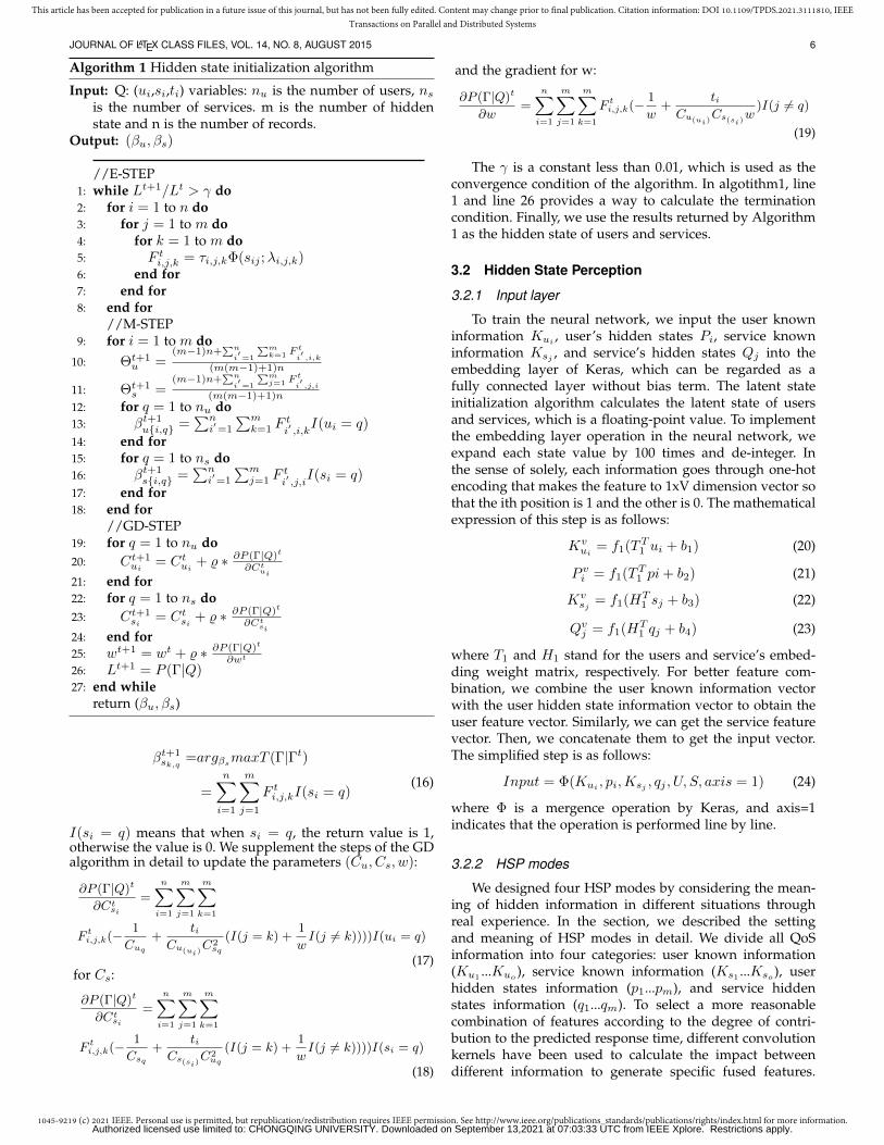
2) The impact of the number of neurons (V)In HSA-Net, we map each information into a 1xV di-

mensional vector. At the same time, we set the number ofchannels of the convolution operation to V. The number ofneurons in the QoSprediction step is 2V, V, and 1. In thissection, we adjusted the value of V to confirm the influenceof different parameters on the model.Approach: We evaluate the running time of HSA-Net whenV takes a different value. It can be seen from Figure 12that as V increases, the learning cost becomes high. In theexperiment, the MAE indicator fluctuates within 0.1, but thecost of learning increases significantly with the increase of V.As illustrated in Figure 10, when V=1024, the training timeis twice that of V=512, and when V=2048, the training timeis nine times that of V=512.Results: The prediction accuracy does not increase signifi-cantly with the increase of V, but the learning cost increasesrapidly. Considering the cost of learning, the default settingof V is 512.

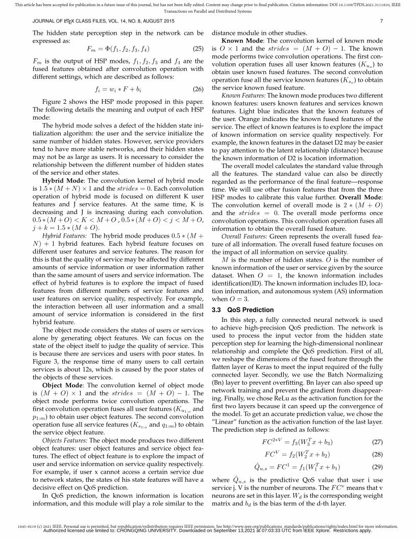
3) The impact of the loss functionApproach: This section compares the performance of theHuber loss function against the MAE (absolute error loss)and MSE (squared error loss) functions.

As shown in Figure 10, the loss function has a greaterimpact on the MAE indicator than the RMSE indicator.Among the compared indicators, the MSE loss function hasthe worst prediction performance, and the MAE functionachieves the highest precision prediction.Results: The MAE loss function has the best predictionperformance because the MAE function can ignore the in-fluence of outliers as much as possible.

The experimental results are summarized in Figure 11.The results show that the MAE function has the best per-formance between MAE and RMSE for the QoS prediction.Through the analysis of the dataset, we discover a phe-nomenon that there are a large number of outliers in theQoS datasets. The response time of most service records isless than 1 second, and the response time of the overtimeservice is 20.

4) The impact of learning rates

0.05 0.10 0.15 0.20Density

0.290.300.310.320.330.340.350.360.370.380.390.400.410.420.430.44

MAE

MSE Huber MAE

0.05 0.10 0.15 0.20Density

1.101.121.141.161.181.201.221.241.261.28

RMSE

MSE Huber MAE

Fig. 11: The impact of loss fuction on the HSA-Net.

0.05 0.10 0.15 0.20Density

0.290.300.310.320.330.340.350.360.370.380.390.400.41

MAE

0.0010.0005

0.005 0.0001

0.05 0.10 0.15 0.20Density

1.101.121.141.161.181.201.221.241.261.281.30

RMSE

0.0010.0005

0.005 0.0001

Fig. 12: The impact of learning rates on the HSA-Net

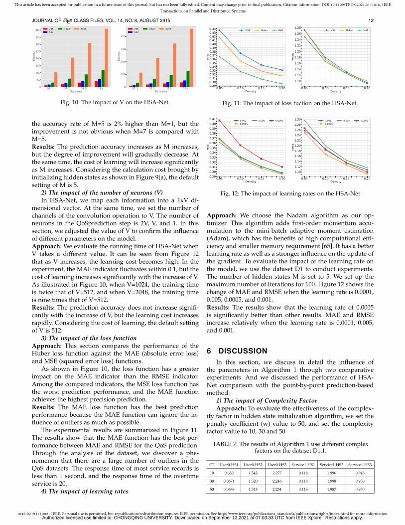
Approach: We choose the Nadam algorithm as our op-timizer. This algorithm adds first-order momentum accu-mulation to the mini-batch adaptive moment estimation(Adam), which has the benefits of high computational effi-ciency and smaller memory requirement [65]. It has a betterlearning rate as well as a stronger influence on the update ofthe gradient. To evaluate the impact of the learning rate onthe model, we use the dataset D1 to conduct experiments.The number of hidden states M is set to 5. We set up themaximum number of iterations for 100. Figure 12 shows thechange of MAE and RMSE when the learning rate is 0.0001,0.005, 0.0005, and 0.001.Results: The results show that the learning rate of 0.0005is significantly better than other results. MAE and RMSEincrease relatively when the learning rate is 0.0001, 0.005,and 0.001.

6 DISCUSSIONIn this section, we discuss in detail the influence of

the parameters in Algorithm 1 through two comparativeexperiments. And we discussed the performance of HSA-Net comparison with the point-by-point prediction-basedmethod.

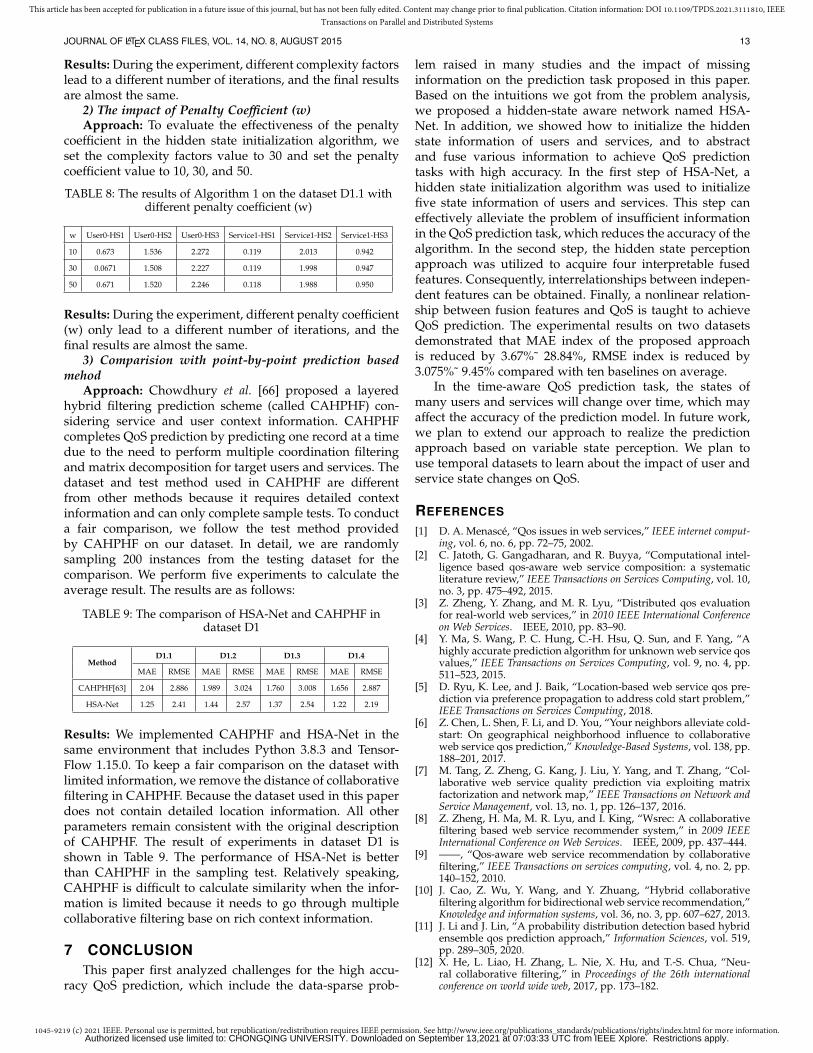
1) The impact of Complexity FactorApproach: To evaluate the effectiveness of the complex-

ity factor in hidden state initialization algorithm, we set thepenalty coefficient (w) value to 50, and set the complexityfactor value to 10, 30 and 50.

TABLE 7: The results of Algorithm 1 use different complexfactors on the dataset D1.1.

CF User0-HS1 User0-HS2 User0-HS3 Service1-HS1 Service1-HS2 Service1-HS3

10 0.680 1.542 2.277 0.118 1.996 0.948

30 0.0671 1.520 2.246 0.118 1.998 0.950

50 0.0668 1.513 2.234 0.118 1.987 0.950





Results: During the experiment, different complexity factorslead to a different number of iterations, and the final resultsare almost the same.

2) The impact of Penalty Coefficient (w)Approach: To evaluate the effectiveness of the penalty

coefficient in the hidden state initialization algorithm, weset the complexity factors value to 30 and set the penaltycoefficient value to 10, 30, and 50.

TABLE 8: The results of Algorithm 1 on the dataset D1.1 withdifferent penalty coefficient (w)

w User0-HS1 User0-HS2 User0-HS3 Service1-HS1 Service1-HS2 Service1-HS3

10 0.673 1.536 2.272 0.119 2.013 0.942

30 0.0671 1.508 2.227 0.119 1.998 0.947

50 0.671 1.520 2.246 0.118 1.988 0.950

Results: During the experiment, different penalty coefficient(w) only lead to a different number of iterations, and thefinal results are almost the same.

3) Comparision with point-by-point prediction basedmehod

Approach: Chowdhury et al. [66] proposed a layeredhybrid filtering prediction scheme (called CAHPHF) con-sidering service and user context information. CAHPHFcompletes QoS prediction by predicting one record at a timedue to the need to perform multiple coordination filteringand matrix decomposition for target users and services. Thedataset and test method used in CAHPHF are differentfrom other methods because it requires detailed contextinformation and can only complete sample tests. To conducta fair comparison, we follow the test method providedby CAHPHF on our dataset. In detail, we are randomlysampling 200 instances from the testing dataset for thecomparison. We perform five experiments to calculate theaverage result. The results are as follows:

TABLE 9: The comparison of HSA-Net and CAHPHF indataset D1


MAE RMSE MAE RMSE MAE RMSE MAE RMSE

CAHPHF[63] 2.04 2.886 1.989 3.024 1.760 3.008 1.656 2.887

HSA-Net 1.25 2.41 1.44 2.57 1.37 2.54 1.22 2.19

Results: We implemented CAHPHF and HSA-Net in thesame environment that includes Python 3.8.3 and Tensor-Flow 1.15.0. To keep a fair comparison on the dataset withlimited information, we remove the distance of collaborativefiltering in CAHPHF. Because the dataset used in this paperdoes not contain detailed location information. All otherparameters remain consistent with the original descriptionof CAHPHF. The result of experiments in dataset D1 isshown in Table 9. The performance of HSA-Net is betterthan CAHPHF in the sampling test. Relatively speaking,CAHPHF is difficult to calculate similarity when the infor-mation is limited because it needs to go through multiplecollaborative filtering base on rich context information.

7 CONCLUSIONThis paper first analyzed challenges for the high accu-

racy QoS prediction, which include the data-sparse prob-

lem raised in many studies and the impact of missinginformation on the prediction task proposed in this paper.Based on the intuitions we got from the problem analysis,we proposed a hidden-state aware network named HSA-Net. In addition, we showed how to initialize the hiddenstate information of users and services, and to abstractand fuse various information to achieve QoS predictiontasks with high accuracy. In the first step of HSA-Net, ahidden state initialization algorithm was used to initializefive state information of users and services. This step caneffectively alleviate the problem of insufficient informationin the QoS prediction task, which reduces the accuracy of thealgorithm. In the second step, the hidden state perceptionapproach was utilized to acquire four interpretable fusedfeatures. Consequently, interrelationships between indepen-dent features can be obtained. Finally, a nonlinear relation-ship between fusion features and QoS is taught to achieveQoS prediction. The experimental results on two datasetsdemonstrated that MAE index of the proposed approachis reduced by 3.67%˜ 28.84%, RMSE index is reduced by3.075%˜ 9.45% compared with ten baselines on average.

In the time-aware QoS prediction task, the states ofmany users and services will change over time, which mayaffect the accuracy of the prediction model. In future work,we plan to extend our approach to realize the predictionapproach based on variable state perception. We plan touse temporal datasets to learn about the impact of user andservice state changes on QoS.

REFERENCES

[1] D. A. Menasce, “Qos issues in web services,” IEEE internet comput-ing, vol. 6, no. 6, pp. 72–75, 2002.

[2] C. Jatoth, G. Gangadharan, and R. Buyya, “Computational intel-ligence based qos-aware web service composition: a systematicliterature review,” IEEE Transactions on Services Computing, vol. 10,no. 3, pp. 475–492, 2015.

[3] Z. Zheng, Y. Zhang, and M. R. Lyu, “Distributed qos evaluationfor real-world web services,” in 2010 IEEE International Conferenceon Web Services. IEEE, 2010, pp. 83–90.

[4] Y. Ma, S. Wang, P. C. Hung, C.-H. Hsu, Q. Sun, and F. Yang, “Ahighly accurate prediction algorithm for unknown web service qosvalues,” IEEE Transactions on Services Computing, vol. 9, no. 4, pp.511–523, 2015.

[5] D. Ryu, K. Lee, and J. Baik, “Location-based web service qos pre-diction via preference propagation to address cold start problem,”IEEE Transactions on Services Computing, 2018.

[6] Z. Chen, L. Shen, F. Li, and D. You, “Your neighbors alleviate cold-start: On geographical neighborhood influence to collaborativeweb service qos prediction,” Knowledge-Based Systems, vol. 138, pp.188–201, 2017.

[7] M. Tang, Z. Zheng, G. Kang, J. Liu, Y. Yang, and T. Zhang, “Col-laborative web service quality prediction via exploiting matrixfactorization and network map,” IEEE Transactions on Network andService Management, vol. 13, no. 1, pp. 126–137, 2016.

[8] Z. Zheng, H. Ma, M. R. Lyu, and I. King, “Wsrec: A collaborativefiltering based web service recommender system,” in 2009 IEEEInternational Conference on Web Services. IEEE, 2009, pp. 437–444.

[9] ——, “Qos-aware web service recommendation by collaborativefiltering,” IEEE Transactions on services computing, vol. 4, no. 2, pp.140–152, 2010.

[10] J. Cao, Z. Wu, Y. Wang, and Y. Zhuang, “Hybrid collaborativefiltering algorithm for bidirectional web service recommendation,”Knowledge and information systems, vol. 36, no. 3, pp. 607–627, 2013.

[11] J. Li and J. Lin, “A probability distribution detection based hybridensemble qos prediction approach,” Information Sciences, vol. 519,pp. 289–305, 2020.

[12] X. He, L. Liao, H. Zhang, L. Nie, X. Hu, and T.-S. Chua, “Neu-ral collaborative filtering,” in Proceedings of the 26th internationalconference on world wide web, 2017, pp. 173–182.





[13] H.-J. Xue, X. Dai, J. Zhang, S. Huang, and J. Chen, “Deep matrixfactorization models for recommender systems.” in IJCAI, vol. 17.Melbourne, Australia, 2017, pp. 3203–3209.

[14] Y. Zhang, C. Yin, Q. Wu, Q. He, and H. Zhu, “Location-awaredeep collaborative filtering for service recommendation,” IEEETransactions on Systems, Man, and Cybernetics: Systems, 2019.

[15] W. Ahmed, Y. Wu, and W. Zheng, “Response time based optimalweb service selection,” IEEE Transactions on Parallel and distributedsystems, vol. 26, no. 2, pp. 551–561, 2013.

[16] J. Li, J. Wang, Q. Sun, and A. Zhou, “Temporal influences-awarecollaborative filtering for qos-based service recommendation,” in2017 IEEE International Conference on Services Computing (SCC).IEEE, 2017, pp. 471–474.

[17] O. G. Uyan and V. C. Gungor, “Qos-aware lte-a downlink schedul-ing algorithm: A case study on edge users,” International Journal ofCommunication Systems, vol. 32, no. 15, p. e4066, 2019.

[18] L. Chen, F. Xie, Z. Zheng, and Y. Wu, “Predicting quality of servicevia leveraging location information,” Complexity, vol. 2019, 2019.

[19] Y. Wu, F. Xie, L. Chen, C. Chen, and Z. Zheng, “An embeddingbased factorization machine approach for web service qos pre-diction,” in International Conference on Service-Oriented Computing.Springer, 2017, pp. 272–286.

[20] S. H. Ghafouri, S. M. Hashemi, and P. C. Hung, “A survey onweb service qos prediction methods,” IEEE Transactions on ServicesComputing, 2020.

[21] Z. Zheng, L. Xiaoli, M. Tang, F. Xie, and M. R. Lyu, “Web serviceqos prediction via collaborative filtering: A survey,” IEEE Transac-tions on Services Computing, 2020.

[22] K. Lee, J. Park, and J. Baik, “Location-based web service qosprediction via preference propagation for improving cold startproblem,” in 2015 IEEE International Conference on Web Services.IEEE, 2015, pp. 177–184.

[23] X. Chen, X. Liu, Z. Huang, and H. Sun, “Regionknn: A scalablehybrid collaborative filtering algorithm for personalized web ser-vice recommendation,” in 2010 IEEE international conference on webservices. IEEE, 2010, pp. 9–16.

[24] Z. Zheng, H. Ma, M. R. Lyu, and I. King, “Qos-aware web servicerecommendation by collaborative filtering,” IEEE Transactions onservices computing, vol. 4, no. 2, pp. 140–152, 2010.

[25] Z. Chen, L. Shen, F. Li, and D. You, “Your neighbors alleviate cold-start: On geographical neighborhood influence to collaborativeweb service qos prediction,” Knowledge-Based Systems, vol. 138, pp.188–201, 2017.

[26] H. Wu, K. Yue, B. Li, B. Zhang, and C.-H. Hsu, “Collaborativeqos prediction with context-sensitive matrix factorization,” FutureGeneration Computer Systems, vol. 82, pp. 669–678, 2018.

[27] J. Zhu, P. He, Z. Zheng, and M. R. Lyu, “Online qos predictionfor runtime service adaptation via adaptive matrix factorization,”IEEE Transactions on Parallel and Distributed Systems, vol. 28, no. 10,pp. 2911–2924, 2017.

[28] C. Wu, W. Qiu, Z. Zheng, X. Wang, and X. Yang, “Qos predictionof web services based on two-phase k-means clustering,” in 2015ieee international conference on web services. IEEE, 2015, pp. 161–168.

[29] Z. Tan and L. He, “An efficient similarity measure for user-based collaborative filtering recommender systems inspired bythe physical resonance principle,” IEEE Access, vol. 5, pp. 27 211–27 228, 2017.

[30] B. Sarwar, G. Karypis, J. Konstan, and J. Riedl, “Item-based collab-orative filtering recommendation algorithms,” in Proceedings of the10th international conference on World Wide Web, 2001, pp. 285–295.

[31] H. Ma, I. King, and M. R. Lyu, “Effective missing data predic-tion for collaborative filtering,” in Proceedings of the 30th annualinternational ACM SIGIR conference on Research and development ininformation retrieval, 2007, pp. 39–46.

[32] H. Sun, Z. Zheng, J. Chen, and M. R. Lyu, “Personalized web ser-vice recommendation via normal recovery collaborative filtering,”IEEE Transactions on Services Computing, vol. 6, no. 4, pp. 573–579,2012.

[33] X. Luo, M. Zhou, S. Li, Z. You, Y. Xia, and Q. Zhu, “A nonnegativelatent factor model for large-scale sparse matrices in recommendersystems via alternating direction method,” IEEE transactions onneural networks and learning systems, vol. 27, no. 3, pp. 579–592,2015.

[34] Y. Shi, M. Larson, and A. Hanjalic, “Collaborative filtering beyondthe user-item matrix: A survey of the state of the art and futurechallenges,” ACM Computing Surveys (CSUR), vol. 47, no. 1, pp.1–45, 2014.

[35] Y. Koren and R. Bell, “Advances in collaborative filtering,” inRecommender systems handbook. Springer, 2015, pp. 77–118.

[36] L. Wu, P. Sun, R. Hong, Y. Ge, and M. Wang, “Collaborative neuralsocial recommendation,” IEEE Transactions on Systems, Man, andCybernetics: Systems, 2018.

[37] L. Ren and W. Wang, “An svm-based collaborative filtering ap-proach for top-n web services recommendation,” Future GenerationComputer Systems, vol. 78, pp. 531–543, 2018.

[38] K. Chen, H. Mao, X. Shi, Y. Xu, and A. Liu, “Trust-aware andlocation-based collaborative filtering for web service qos predic-tion,” in 2017 IEEE 41st Annual Computer Software and ApplicationsConference (COMPSAC), vol. 2. IEEE, 2017, pp. 143–148.

[39] M. Tang, Y. Jiang, J. Liu, and X. Liu, “Location-aware collaborativefiltering for qos-based service recommendation,” in 2012 IEEE 19thinternational conference on web services. IEEE, 2012, pp. 202–209.

[40] J. Liu, M. Tang, Z. Zheng, X. Liu, and S. Lyu, “Location-aware andpersonalized collaborative filtering for web service recommenda-tion,” IEEE Transactions on Services Computing, vol. 9, no. 5, pp.686–699, 2015.

[41] D. Ryu, K. Lee, and J. Baik, “Location-based web service qos pre-diction via preference propagation to address cold start problem,”IEEE Transactions on Services Computing, 2018.

[42] Y. Feng and B. Huang, “Cloud manufacturing service qos pre-diction based on neighbourhood enhanced matrix factorization,”Journal of Intelligent Manufacturing, pp. 1–12, 2018.

[43] Y. Koren, R. Bell, and C. Volinsky, “Matrix factorization techniquesfor recommender systems,” Computer, vol. 42, no. 8, pp. 30–37,2009.

[44] X. Luo, H. Wu, H. Yuan, and M. Zhou, “Temporal pattern-awareqos prediction via biased non-negative latent factorization oftensors,” IEEE transactions on cybernetics, vol. 50, no. 5, pp. 1798–1809, 2019.

[45] X. Luo, M. Zhou, S. Li, Y. Xia, Z.-H. You, Q. Zhu, and H. Leung,“Incorporation of efficient second-order solvers into latent factormodels for accurate prediction of missing qos data,” IEEE transac-tions on cybernetics, vol. 48, no. 4, pp. 1216–1228, 2017.

[46] X. Luo, M. Zhou, Y. Xia, Q. Zhu, A. C. Ammari, and A. Alab-dulwahab, “Generating highly accurate predictions for missingqos data via aggregating nonnegative latent factor models,” IEEEtransactions on neural networks and learning systems, vol. 27, no. 3,pp. 524–537, 2016.

[47] D. WU, Q. He, X. Luo, M. Shang, Y. He, and G. Wang, “Aposterior-neighborhood-regularized latent factor model for highlyaccurate web service qos prediction,” IEEE Transactions on ServicesComputing, 2019.

[48] Z. Luo, L. Liu, J. Yin, Y. Li, and Z. Wu, “Latent ability model: Agenerative probabilistic learning framework for workforce analyt-ics,” IEEE Transactions on Knowledge and Data Engineering, vol. 31,no. 5, pp. 923–937, 2018.

[49] D. Kim, C. Park, J. Oh, S. Lee, and H. Yu, “Convolutional matrixfactorization for document context-aware recommendation,” inProceedings of the 10th ACM conference on recommender systems, 2016,pp. 233–240.

[50] R. Xiong, J. Wang, Z. Li, B. Li, and P. C. Hung, “Personalized lstmbased matrix factorization for online qos prediction,” in 2018 IEEEInternational Conference on Web Services (ICWS). IEEE, 2018, pp.34–41.

[51] X. Zhao, Y. Chen, J. Guo, and D. Zhao, “A spatial-temporal atten-tion model for human trajectory prediction,” IEEE/CAA Journal ofAutomatica Sinica, vol. 7, no. 4, pp. 965–974, 2020.

[52] X. Hou, K. Wang, C. Zhong, and Z. Wei, “St-trader: A spatial-temporal deep neural network for modeling stock market move-ment,” IEEE/CAA Journal of Automatica Sinica, vol. 8, no. 5, pp.1015–1024, 2021.

[53] H. Wu, Z. Zhang, J. Luo, K. Yue, and C.-H. Hsu, “Multipleattributes qos prediction via deep neural model with contexts,”IEEE Transactions on Services Computing, 2018.

[54] W. Li, Y. Xia, M. Zhou, X. Sun, and Q. Zhu, “Fluctuation-aware andpredictive workflow scheduling in cost-effective infrastructure-as-a-service clouds,” IEEE Access, vol. 6, pp. 61 488–61 502, 2018.

[55] J. Bi, H. Yuan, and M. Zhou, “Temporal prediction of multi-application consolidated workloads in distributed clouds,” IEEETransactions on Automation Science and Engineering, vol. 16, no. 4,pp. 1763–1773, 2019.

[56] R. Xiong, J. Wang, N. Zhang, and Y. Ma, “Deep hybrid collabo-rative filtering for web service recommendation,” Expert systemswith Applications, vol. 110, pp. 191–205, 2018.





[57] Y. Yin, L. Chen, Y. Xu, J. Wan, H. Zhang, and Z. Mai, “Qos pre-diction for service recommendation with deep feature learning inedge computing environment,” Mobile Networks and Applications,pp. 1–11, 2019.

[58] J. S. Breese, D. Heckerman, and C. Kadie, “Empirical analysisof predictive algorithms for collaborative filtering,” arXiv preprintarXiv:1301.7363, 2013.

[59] J. M. Hernandez-Lobato, N. Houlsby, and Z. Ghahramani, “Prob-abilistic matrix factorization with non-random missing data,” inInternational Conference on Machine Learning, 2014, pp. 1512–1520.

[60] D. Wu, X. Luo, M. Shang, Y. He, G. Wang, and X. Wu, “Adata-characteristic-aware latent factor model for web services qosprediction,” IEEE Transactions on Knowledge and Data Engineering,2020.

[61] S. Sedhain, A. K. Menon, S. Sanner, and L. Xie, “Autorec: Au-toencoders meet collaborative filtering,” in Proceedings of the 24thinternational conference on World Wide Web, 2015, pp. 111–112.

[62] M. I. Smahi, F. Hadjila, C. Tibermacine, and A. Benamar, “A deeplearning approach for collaborative prediction of web service qos,”Service Oriented Computing and Applications, vol. 15, no. 1, pp. 5–20,2021.

[63] J. Demsar, “Statistical comparisons of classifiers over multiple datasets,” Journal of Machine learning research, vol. 7, no. Jan, pp. 1–30,2006.

[64] A. Benavoli, G. Corani, and F. Mangili, “Should we really use post-hoc tests based on mean-ranks?” The Journal of Machine LearningResearch, vol. 17, no. 1, pp. 152–161, 2016.

[65] D. P. Kingma and J. Ba, “Adam: A method for stochastic optimiza-tion,” arXiv preprint arXiv:1412.6980, 2014.

[66] R. R. Chowdhury, S. Chattopadhyay, and C. Adak, “Cahphf:Context-aware hierarchical qos prediction with hybrid filtering,”IEEE Transactions on Services Computing, 2020.

ZiLiang Wang He was received the B.S. degreefrom Nanchang Hangkong University, Jiangxi,China, in 2017. He is currently pursuing the Ph.Ddegree in software engineering in ChongqingUniversity, Chongqing, China. His current re-search interests include service computing,smart city and system structure.

Meng Yan He is now an Assistant Professorat the School of Big Data and Software Engi-neering, Chongqing University, China. Prior tojoining Chongqing University, he was a Postdocat Zhejiang University. He got his Ph.D degreein June 2017 from Chongqing University, China.His current research focuses on how to improvedevelopers’ productivity, how to improve soft-ware quality and how to reduce the effort duringsoftware development by analyzing rich softwarerepository data.

XiaoHong Zhang He received the M.S. degreein applied mathematics and the Ph.D. degree incomputer software and theory from ChongqingUniversity, China, in 2006. He is currently aProfessor and the Vice Dean of the School ofBig Data and Software Engineering, ChongqingUniversity. His current research interests includedata mining of software engineering, topic mod-eling, image semantic analysis, and video anal-ysis. He has authored over 50 scientific articlesand some of them are published in some author-

itative journals and conferences, such as the IEEE TRANSACTIONSON PATTERN ANALYSIS AND MACHINE INTELLIGENCE, the IEEETRANSACTIONS ON IMAGE PROCESSING, PR, PRL, JSS, and IST.

Ling Xu Ling Xu was born in 1975 and receivedher B.S. in Hefei University of Technology in1998, and her M.S. degree in software engineer-ing in 2004. She received her Ph.D. degree incomputer science technology from ChongqingUniversity, PR China in 2009. She is currently anAssociate Professor of the School of Big Dataand Software Engineering, Chongqing Univer-sity. Her research interests include data miningof software engineering, topic modeling, and im-age processing.

Dan Yang He was received the B.Eng. degree inautomation, the M.S. degree in applied mathe-matics, and the Ph.D. degree in machinery man-ufacturing and automation from Chongqing Uni-versity, Chongqing. From 1997 to 1999, he helda postdoctoral position at the University of Elec-troCommunications, Tokyo, Japan. He is cur-rently the President of Southwest Jiaotong Uni-versity. He is also a Professor with the School ofBig Data and Software Engineering, ChongqingUniversity. He has authored over 100 scientific

articles and some of them are published in some authoritative journalsand conferences, such as the IEEE TRANSACTIONS ON PATTERNANALYSIS AND MACHINE INTELLIGENCE, CVPR, and BMVC. Hisresearch interests include computer vision, image processing, patternrecognition, software engineering, and scientific computing.


Documents

ATEX CLASS FILES, VOL. 14, NO. 8, AUGUST 2015 1 HSA-Net