ATENEO STUDENT BUSINESS REVIEWgsb.ateneo.edu/wp-content/uploads/2015/02/techne_4.pdf · ATENEO STUDENT BUSINESS REVIEW 5 Message from Editor Techne is a magazine about numbers, making

2ATENEO STUDENT BUSINESS REVIEW

ATENEO STUDENT BUSINESS REVIEW3

Message from the Dean

Congratulations once again to the Operations Cluster for this back-to-back Techne 3 and Techne 4 publication.

Once more, the students, faculty, and Cluster Chair have proven their capability and commitment to produce a series of student papers that reflect their applied learning in quantitative and operations management issues.

The variety of topics in Techne 3 and 4 has again demonstrated the usefulness and applicability of topics in the Operations Management (Opeman) cluster courses to any industry or any small, medium, or large company/institution.

The inclusion of some green technology-related topics is a welcome development because they are very relevant to the University’s thrust on

environment and development, AGSB’s research agenda, and our Mulat Diwa’s Cura Kalikasan project.

May the Operations Cluster, with its talented and committed faculty and leaders, continue to lead in the publication of student papers. Please continue to teach and inspire the students so they can learn more, do more, publish more, and do better.

Alberto L. BuenviajeDean

Once more, the students, faculty, and Cluster Chair have proven their capability and commitment to produce a series of student papers that reflect their applied learning in quantitative and operations management issues.


Message from the Operations Cluster HeadCongratulations to the AGSB Operations Cluster for coming up with the back-to-back issues, Techne 3 and Techne 4. Also, a warm welcome to our readers and friends to the 3rd and 4th editions of our magazine!

These two issues were the output of 45 MBA student-authors whose contributions focused on the “Green” theme, which is aligned with our school’s emphasis on nation-building. As in the first two issues, we compiled our MBA students’ projects in Applied Management Science and Operations Management. The potentials of the Applied Management Science and Operations Management tools in improving our workplaces and daily lives are limitless. So in this issue, side-by-side articles on the power crisis in Mindanao and the waste management system in the Payatas dumpsite, are equally interesting write-ups on tikoy, shipping costs of computers to public schools, and even laundry concerns.

As always, I convey my heartfelt gratitude to my colleagues in the Operations Cluster for their efforts to encourage innovation, and to continuously motivate and guide our MBA students.

Thank you to all and happy reading!

Ralph AnteProfessor and Operations Cluster ChairAteneo Graduate School of Business

As always, I convey my heartfelt gratitude to my colleagues in the Operations Cluster for their efforts to encourage innovation, and to continuously motivate and guide our MBA students.


Message from EditorTechne is a magazine about numbers, making it distinct from other management publications. Additionally, you will find this particular issue unique. Let me count the ways – by way of numbers, of course:

2 Means this is a double issue. The front cover is Techne 4. Flip the page around and, surprise, the front cover becomes Techne 3.

2 The Operations Cluster manages a number of AGSB technically-oriented courses. Organized by the Cluster, this magazine focuses on two courses: Management Science and Operations Management.

2 The number of types of numbers presented: constants and variables. Of course, the variables are identified with the “let x =” expression.

3 Articles are trilingual. Although mostly in English, you will find a smattering of Greek letters such as mu, lambda, rho, sigma in a few places, plus a dash of Chinese.

13 The number of articles in this publication, sufficiently large to cover a wide range of technical applications for large corporations, government, schools, small and medium enterprises (SMEs), entrepreneurs, and for corporate social responsibility (CSR) initiatives. Ideas are aplenty: how to best move people and things from point A to point B, how to justify green initiatives, how to reduce time, and how to optimize resources. My personal favorite is the remarkable application of technical tools in the life of Carmina. Hopefully you will find at least one article that will match your interest.

25 The number of applications of mathematical tools (models, processes, concepts, formulas, diagrams, Excel templates) the students had to learn for the articles. Specifically, these consist of six applications of Monte Carlo Simulation, five of Linear Programming, four of Linear Regression, three each of Queuing Models and Project Management, and one each of Inventory Management, Integer Programming, Process Improvement, and Quality Management.

45 The number of AGSB students who collaborated to write the articles. Many are engineers, accountants, and IT graduates, but you will be surprised to know how many lawyers, doctors, and politicians were involved as well.

510 Nanometers, the wavelength of visible green light in the color spectrum, right below the blue light. Management of the interaction and impact of humans on the environment is signified by green, the theme of Techne 3.

0, 1, 1, 2, 3, 5, 8, 13, 21, 34, 55, 89, 144, … Fibonacci sequence is an integer sequence where each subsequent number is the sum of the previous two. We do not have this yet in the current issue but with the way things are moving, you may be able to read about its application, perhaps in the field of decision theory, in a future Techne article.

Ed LegaspiEditorTechne: Managing through NumbersAteneo Graduate School of Business


GLYFORD JON T. FU

Kung Hei Fat Choy*

Tikoy, Anyone?* Chinese New Year’s greeting in Cantonese, also Gong Xi Fa Cai in Mandarin.


Introduction

GSW ENTERPRISES MAKES and sells glutinous rice food (known as nian gao or tikoy in the Philippines) during the Lunar New Year festival season. This undertaking is its contribution to the Chinese New Year festivities in Manila. To make tikoy extra special, GSW only makes it once a year, during the months of January and February.

GSW makes two variants of tikoy: white and brown. Each variant has different sizes: small, medium, large, and extra large. Based on past sales performance, the best seller is the medium-sized white variant. In fact, demand for this item every Chinese New Year season is virtually limitless. This situation is satisfactory, but management could have wished that the other variants would sell as well as the best seller.

Given the conservative character of the owners and the once-a-year nature of the venture, management typically adopts a style that relies on “rule of thumb” guesses and estimates when ordering ingredients and hiring manpower. This approach implies that, year after year, the same amounts of ingredients are ordered and the same number of workers is hired. Any shortage or surplus is charged as part of sales cost, and any under- or overutilization of labor is not taken into consideration.

Currently, the children of the owners are incorporating their school-acquired knowledge into the business as a way of helping run the operations. The children believe that the business can be improved when certain variables are changed, such as prices, direct costs, minimum number of orders required, and number of workers to be hired. GSW has been operating for the past 25 years; thus, it has a strong brand equity, and exerts reasonable control over the aforementioned variables. Therefore, management has reason to believe that the suggestions are feasible and realistic.

On average, demand for tikoy remained steady for the past four years. However, management knows that it could have served more retailers without losing money if one factor existed: improved shelf life of tikoy. The typical shelf life of tikoy (unrefrigerated) is from five to seven days. Relying on the market trend for tikoy during Chinese New Year and having confidence in the quality of its product enable GSW to guarantee to retailers/resellers that tikoy purchased from GSW would be sold before the expiration date. As a result, accepting and honoring sales returns (i.e., bad

Given the conservative character of the owners and the once-a-year nature of

the venture, management typically adopts a style that relies on “rule of thumb”

guesses and estimates when ordering ingredients and hiring manpower.

Tikoy, Anyone?


orders) from retailers, whose sum is equal to the cost of all unsold tikoy after the expiration date, has become a customer policy at GSW. This superior guarantee is one of the reasons why numerous retailers patronize GSW.

Nevertheless, such a guarantee has a downside. Aside from absorbing all losses from unsold products, GSW cannot make the tikoy in advance (i.e., to meet last-minute and surprise orders) and then stock it for a long period. Thus, GSW only makes the tikoy based on every order of the customer (by phone), and last-minute additional orders are turned down. The volume of additional demand that has been declined is significant.

GSW decided to invest in a vacuum packing machine that would vacuum seal the tikoy to improve its shelf life. Based on tests and trial runs, the shelf life of the tikoy would improve from five to seven days to 12 to 15 days if it were vacuum sealed. This option is favorable for two reasons: first, a longer shelf life would mean less sales returns and fewer losses. Second, GSW may now be able to make additional tikoy and stock the item, thus allowing last-minute demand to be met.

Optimization Model

Based on the given scenario, several variables and limitations can be identified. One variable is that making a specific kind of tikoy requires a different mix of various ingredients. These ingredients are ordered in but in limited quantities due to budget and storage concerns. In addition, a specific ceiling is imposed in terms of demand, which implies that over-produced varieties would remain unsold.

Thus, the main goal is to identify the best mix of tikoy variety to be produced to obtain the highest possible profit. Considering the aforementioned points, linear programming represents the best optimization tool for this type of problem.

As previously noted, GSW makes two variants of tikoy, white and brown, and each variant comes in four sizes: small, medium, large, and extra large. The contribution margin of each kind of tikoy is presented in Table 1. The desired outcome is to have the best possible mix of products to be made to yield the highest possible profit. Therefore, this situation is a maximization problem.

The vacuum packing machine proved to be a significant investment. Aside from the acquisition cost, direct cost increased as a result of purchasing the plastic needed for the vacuum seal, and the additional labor required to do the sealing for each tikoy.

The task is to determine the current optimum product mix using the estimates, and how the current resources will be maximized.


Contribution Margin

TIKOY WS 5

TIKOY WM 10

TIKOY WL 15

TIKOY WX 20

TIKOY BS 5

TIKOY BM 10

TIKOY BL 15

TIKOY BX 20

Tikoy WS

Tikoy WM

Tikoy WL

Tikoy WX

Tikoy BS

Tikoy BM

Tikoy BL

Tikoy BX Available

Ingredient A 0.17 0.33 0.50 0.67 0.17 0.33 0.50 0.67 12,000

Ingredient B 0.17 0.33 0.50 0.67 0.17 0.33 0.50 0.67 12,000

Ingredient C 0.17 0.33 0.50 0.67 0.17 0.33 0.50 0.67 12,000

Ingredient D 0.00 0.01 0.01 0.01 0.00 0.01 0.01 0.01 300

Ingredient E - - - - 0.05 0.10 0.15 0.20 1,500

Table 1. Contribution Margins of the Different Products (Php/kg)

The limitations of the raw materials are shown in Table 2. Making tikoy requires the use of ingredients A, B, C, and D. For the brown variant, an additional ingredient E is required. Given the financial constraints and warehousing concerns, only 12,000 kg of ingredients A, B, and C are available in one production season. The quantity of ingredients D and E is dependent on A, B, and C (in terms of proportion); hence, the available amounts are demonstrated accordingly.

Table 2. Raw Material Limitations (kg) Table 2. Raw Material Limitations (kg)

Production runs are only done once a year; thus, all employees in production are contractual. The headcount is in equivalent units (not the actual number of employees) because not all employees are present during the duration of the production run.

Labor is distributed to two broad divisions: production and packaging. The production phase involves mixing, cooking, and setting. Meanwhile, packaging involves vacuum sealing, boxing, and stacking. The production and packaging of the products are done in batches; hence, the total time per batch is divided into the number of units per batch and is assigned to each unit of product. The labor data are summarized in Tables 3 and 4.


Breakdown ofLabor Hours

Days Hours/Day Headcount Total

Production 10 24 12 2880

Packaging 10 24 12 2880

Tikoy WS

Tikoy WM

Tikoy WL

Tikoy WX

Tikoy BS

Tikoy BM

Tikoy BL

Tikoy BX Available

Time in Production (hr)

0.02 0.02 0.03 0.04 0.02 0.02 0.03 0.04 2,880

Time in Packaging and

Sealing (hr)0.05 0.05 0.05 0.05 0.05 0.05 0.05 0.05 2,880

Total 0.07 0.07 0.08 0.09 0.07 0.07 0.08 0.09 -

Table 3. Labor Limitations

Table 4. Labor Allocation for the Different Products

The demand limitations are shown in Table 5. Virtually no cap for demand for Tikoy WM is evident because it is the most saleable product. Based on prior period sales runs, Tikoy BX is the least saleable product. Nevertheless, the company continues to produce Tikoy

BX due to continuing demand for the product.

The other demand constraints are drawn from past records and sales experience. The amounts are rounded off to the nearest tens for the purpose of convenience.

Table 5. Constraints on Product Demand (kg)

Current Demand Tikoy WS

Tikoy WM

Tikoy WL

Tikoy WX

Tikoy BS

Tikoy BM

Tikoy BL

Tikoy BX

Minimum Demand 2,700 2,700 720 270 2,250 2,250 600 240

Maximum Demand 9,520 0 5,360 4,500 8,500 16,820 4,980 4,250


As shown in Table 6, the optimal production mix generated by Solver is as follows: WS=2,700 kg, WM=2,700 kg, WL=5,360 kg, WX=4,500 kg, BS=2,250 kg, BM=2,250 kg, BL=2,023 kg, and BX=4,250 kg. The maximum profit for this production is Php360,000.

Conclusions

The optimal production quantity for products WS, WM, BS, and BM is set at minimum demand. Conversely, the production quantity for products WL, WX, and BX is stretched up to their respective maximum demand. BL is the only product that is optimized at a level that is neither its minimum nor maximum demand. WM turned out to be a surprise because the optimizer chose to produce it at minimum demand, although an open-ended maximum demand had been set. Setting the minimum at higher levels will result in reducing the optimal level of the other products. The maximum profit remains at Php360,000.

Ingredients A, B, C, and E are limiting (i.e., they control the optimum

production). If additional profits are desired, higher quantities of the finished products will have to be produced from the additional increments of these ingredients. From the current level of 12,000 kg each for ingredients A, B, and C, an increase for each by 6,000 kg (bringing the total available for each ingredient to 18,000 kg) will raise the optimal profit to Php540,000 (Table 7). At this level, WM shoots up to 16,265 kg, BL reaches the maximum limit of 4,980 kg, and the rest of the products remain at their current optimal levels.

The current optimal requirement for ingredient D is only 200 kg, leaving 100 kg unused. However, as the quantities of ingredients A, B, and C are increased, the surplus of D is reduced until it becomes limiting itself at the point where 18,000 kg each of A, B, and C are used.

The current optimal production only utilized 3 workers in production and 6 workers in packaging, in contrast to the 12 workers who were used in the optimization program.

Thus, greater profits will be realized by obtaining an additional supply of ingredients A, B, C, and E, as well as reducing labor to the level determined by Solver.

Setting the minimum at higher levels will result in reducing the

optimal level of the other products.


Cons

trai

nt C

oeffi

cien

ts

ING

RED

IEN

T A

0.17

0.33

0.50

0.67

0.17

0.33

0.50

0.67

ING

RED

IEN

T B

0.17

0.33

0.50

0.67

0.17

0.33

0.50

0.67

ING

RED

IEN

T C

0.17

0.33

0.50

0.67

0.17

0.33

0.50

0.67

ING

RED

IEN

T D

0.00

0.01

0.01

0.01

0.00

0.01

0.01

0.01

ING

RED

IEN

T E

--

--

0.05

0.10

0.15

0.20

TIM

E IN

PRO

DU

CTIO

N0.

020.

020.

030.

040.

020.

020.

030.

04TI

ME

IN P

ACK

AG

ING

0.05

0.05

0.05

0.05

0.05

0.05

0.05

0.05

MIN

DEM

AN

D F

OR

WS

1.00

MIN

DEM

AN

D F

OR

WM

1.00

MIN

DEM

AN

D F

OR

WL

1.00

MIN

DEM

AN

D F

OR

WX

1.00

MIN

DEM

AN

D F

OR

BS1.

00M

IN D

EMA

ND

FO

R BM

1.00

MIN

DEM

AN

D F

OR

BL1.

00M

IN D

EMA

ND

FO

R BX

1.00

MA

X D

EMA

ND

FO

R W

S1.

00M

AX

DEM

AN

D F

OR

WL

1.00

MA

X D

EMA

ND

FO

R W

X1.

00M

AX

DEM

AN

D F

OR

BS1.

00M

AX

DEM

AN

D F

OR

BM1.

00M

AX

DEM

AN

D F

OR

BL1.

00M

AX

DEM

AN

D F

OR

BX1.

00

Cons

trai

nt R

esul

tsU

sed

Ava

ilabl

eU

nuse

d

ING

RED

IEN

T A

450

900

2680

3000

375

750

1012

2833

1200

012

000

0IN

GRE

DIE

NT

B45

090

026

8030

0037

575

010

1228

3312

000

1200

00

ING

RED

IEN

T C

450

900

2680

3000

375

750

1012

2833

1200

012

000

0IN

GRE

DIE

NT

D8

1545

506

1317

4720

030

010

0IN

GRE

DIE

NT

E0

00

011

322

530

485

014

9115

009

TIM

E IN

PRO

DU

CTIO

N41

5416

118

034

4561

170

745

2880

2135

TIM

E IN

PA

CKA

GIN

G14

214

228

123

611

811

810

622

313

6728

8015

13M

IN D

EMA

ND

FO

R W

S27

000

00

00

00

2700

2700

0M

IN D

EMA

ND

FO

R W

M0

2700

00

00

00

2700

2700

0M

IN D

EMA

ND

FO

R W

L0

053

600

00

00

5360

720

-464

0M

IN D

EMA

ND

FO

R W

X0

00

4500

00

00

4500

270

-423

0M

IN D

EMA

ND

FO

R BS

00

00

2250

00

022

5022

500

MIN

DEM

AN

D F

OR

BM0

00

00

2250

00

2250

2250

0M

IN D

EMA

ND

FO

R BL

00

00

00

2023

020

2360

0-1

423

MIN

DEM

AN

D F

OR

BX0

00

00

00

4250

4250

240

-401

0M

AX

DEM

AN

D F

OR

WS

2700

00

00

00

027

0095

2068

20M

AX

DEM

AN

D F

OR

WL

00

5360

00

00

053

6053

600

MA

X D

EMA

ND

FO

R W

X0

00

4500

00

00

4500

4500

0M

AX

DEM

AN

D F

OR

BS0

00

022

500

00

2250

8500

6250

MA

X D

EMA

ND

FO

R BM

00

00

022

500

022

5016

820

1457

0M

AX

DEM

AN

D F

OR

BL0

00

00

020

230

2023

4980

2957

MA

X D

EMA

ND

FO

R BX

00

00

00

042

5042

5042

500

Pro

blem

Obj

ecti

veTo

tal

12

34

56

78

Obj

ectiv

eD

ecis

ion

Var

iabl

e ID

TIKO

Y W

STI

KOY

WM

TIKO

Y W

LTI

KOY

WX

TIKO

Y BS

TIKO

Y BM

TIKO

Y BL

TIKO

Y BX

Qua

ntity

(lea

ve b

lank

)27

0027

0053

6045

00

2250

2250

202.

3333

3342

50U

nit c

oeffi

cien

ts5

1015

205

1015

20To

tal O

bjec

tive

1350

027

000

8040

090

000

1125

022

500

3035

085

000

360,

000

SOLV

ER T

EMP

LATE

Cas

e P

robl

em N

ame:

Tab

le 6

. Opt

imal

Pro

duct

ion

Mix


SOLV

ER T

EMP

LATE

Cas

e P

robl

em N

ame:

Tab

le 7

. Opt

imal

Pro

duct

ion

Mix

at H

ighe

r Pro

duct

ion

Leve

l

Cons

trai

nt C

oeffi

cien

ts

ING

RED

IEN

T A

0.17

0.33

0.50

0.67

0.17

0.33

0.50

0.67

ING

RED

IEN

T B

0.17

0.33

0.50

0.67

0.17

0.33

0.50

0.67

ING

RED

IEN

T C

0.17

0.33

0.50

0.67

0.17

0.33

0.50

0.67

ING

RED

IEN

T D

0.00

0.01

0.01

0.01

0.00

0.01

0.01

0.01

ING

RED

IEN

T E

--

--

0.05

0.10

0.15

0.20

TIM

E IN

PRO

DU

CTIO

N0.

020.

020.

030.

040.

020.

020.

030.

04TI

ME

IN P

ACK

AG

ING

0.05

0.05

0.05

0.05

0.05

0.05

0.05

0.05

MIN

DEM

AN

D F

OR

WS

1.00

MIN

DEM

AN

D F

OR

WM

1.00

MIN

DEM

AN

D F

OR

WL

1.00

MIN

DEM

AN

D F

OR

WX

1.00

MIN

DEM

AN

D F

OR

BS1.

00M

IN D

EMA

ND

FO

R BM

1.00

MIN

DEM

AN

D F

OR

BL1.

00M

IN D

EMA

ND

FO

R BX

1.00

MA

X D

EMA

ND

FO

R W

S1.

00M

AX

DEM

AN

D F

OR

WL

1.00

MA

X D

EMA

ND

FO

R W

X1.

00M

AX

DEM

AN

D F

OR

BS1.

00M

AX

DEM

AN

D F

OR

BM1.

00M

AX

DEM

AN

D F

OR

BL1.

00M

AX

DEM

AN

D F

OR

BX1.

00

Cons

trai

nt R

esul

tsU

sed

Ava

ilabl

eU

nuse

d

ING

RED

IEN

T A

450

5422

2680

3000

375

750

2490

2833

1800

018

000

0IN

GRE

DIE

NT

B45

054

2226

8030

0037

575

024

9028

3318

000

1800

00

ING

RED

IEN

T C

450

5422

2680

3000

375

750

2490

2833

1800

018

000

0IN

GRE

DIE

NT

D8

9045

506

1342

4730

018

000

1770

0IN

GRE

DIE

NT

E0

00

011

322

574

785

019

3520

0066

TIM

E IN

PRO

DU

CTIO

N41

325

161

180

3445

149

170

1105

2880

1775

TIM

E IN

PA

CKA

GIN

G14

285

428

123

611

811

826

122

322

3428

8064

6M

IN D

EMA

ND

FO

R W

S27

000

00

00

00

2700

2700

0M

IN D

EMA

ND

FO

R W

M0

1626

50

00

00

016

265

2700

-135

65M

IN D

EMA

ND

FO

R W

L0

053

600

00

00

5360

720

-464

0M

IN D

EMA

ND

FO

R W

X0

00

4500

00

00

4500

270

-423

0M

IN D

EMA

ND

FO

R BS

00

00

2250

00

022

5022

500

MIN

DEM

AN

D F

OR

BM0

00

00

2250

00

2250

2250

0M

IN D

EMA

ND

FO

R BL

00

00

00

4980

049

8060

0-4

380

MIN

DEM

AN

D F

OR

BX0

00

00

00

4250

4250

240

-401

0M

AX

DEM

AN

D F

OR

WS

2700

00

00

00

027

0095

2068

20M

AX

DEM

AN

D F

OR

WL

00

5360

00

00

053

6053

600

MA

X D

EMA

ND

FO

R W

X0

00

4500

00

00

4500

4500

0M

AX

DEM

AN

D F

OR

BS0

00

022

500

00

2250

8500

6250

MA

X D

EMA

ND

FO

R BM

00

00

022

500

022

5016

820

1457

0M

AX

DEM

AN

D F

OR

BL0

00

00

049

800

4980

4980

0M

AX

DEM

AN

D F

OR

BX0

00

00

00

4250

4250

4250

0

Pro

blem

Obj

ecti

veTo

tal

12

34

56

78

Obj

ectiv

eD

ecis

ion

Var

iabl

e ID

TIKO

Y W

STI

KOY

WM

TIKO

Y W

LTI

KOY

WX

TIKO

Y BS

TIKO

Y BM

TIKO

Y BL

TIKO

Y BX

Qua

ntity

(lea

ve b

lank

)27

0016

265

5360

4500

22

5022

5049

8042

50U

nit c

oeffi

cien

ts5

1015

205

1015

20To

tal O

bjec

tive

1350

016

2650

8040

090

000

1125

022

500

7470

085

000

540,

000


of

ATTY. ALDER DELLORODIANAJIYOUN JANGPAUL LAZARO, CPA, CIAMACY MONSOD

Quantiin the life

Carmina


ATTY. ALDER DELLORODIANAJIYOUN JANGPAUL LAZARO, CPA, CIAMACY MONSOD

PERT-CPM: Rebuilding the Family Home

eorgie Reyes and his wife Carmina Florentino-Reyes are having their second to fourth babies within four months. An ultrasound test done on

Carmina showed that the couple are expecting triplets! Georgie, Carmina, and their daughter Phoebe are living in a one-story, two-bedroom house that sits on a 110-sq.m. lot and with total floor area of 80 sq.m. With the pending birth of their triplets, the couple decided that they needed to have more space to provide separate rooms for each of their children.

Georgie and Carmina plan to have their house rebuilt to a two-story house with five bedrooms in a span of four months. Georgie decided to consult with his architect friend Rico who has his own home building and renovation business to discuss their plan and look for options to

ensure that the house is ready by the time their new babies are born.

According to Rico, a project of this magnitude would take approximately 4.5 months (eight hours a day, six-day workweek) to complete and PhP2.48 million to finance. Can the project be fast-tracked from 4.5 months to 4 months just in time for the babies’ birth, while limiting the cost to under PhP3 million?

Rico provided Georgie with a project plan to give him an idea of the things that need to be accomplished to complete the project before Carmina gives birth. Rico also reminded the couple about a method— the Quanti concept PERT-CPM—that allows them to estimate the feasibility of the home rebuilding project, and determine if the project deals with their budget constraint. Table 1 presents the list of activities for the home renovation.

G

Carmina

Table 1. Schedule of Activities and Costs Incomplete predecessors: J after E,H; K after F,G,J; O after L,M,N

ProcessRegular Crashed Incremental

Cost per DayPredecessor Time (days) Cost Time (days) Cost

A Transfer all furnitures and appliances to a rented house None 2 50,000 2 50,000

B Demolish current structure A 14 50,000 10 80,000 7,500

C Build foundation for the new house B 20 400,000 20 400,000

D Prepare and build walls for the first floor C 7 100,000 6 105,000 5,000

E Install beams for the second floor D 10 90,000 8 110,000 10,000

F Install plumbing B 3 200,000 3 200,000

G Install electrical lines and breakers B 7 150,000 6 155,000 5,000

H Prepare and build walls for the second floor C 7 250,000 7 250,000

I Install windows and doors of the first floor C 3 270,000 3 270,000

J Install windows and doors of the second floor E, H 3 270,000 3 270,000

K Final finishing of rough surfaces F, G, I, J 30 350,000 26 400,000 12,500

L Paint interior of the house K 30 250,000 25 300,000 10,000

M Paint exterior of the house K 14 100,000 11 130,000 10,000

N Build and install roof of the house J 4 300,000 2 315,000 7,500

O Move back furnitures and fixtures of Georgie and Carmina L, M, N 2 20,000 2 20,000

Total cost 2,850,000 3,055,000


The objective is to complete the home construction process in four months to coincide with the birth of the couple’s children. The construction process applying regular time and costs to the project activities is expected to take more than four months. The next step is to crash the project time to four months at the least cost increase possible.

Figure 1. Network Diagram

Figure 1 presents the Network Diagram for the project. Table 2 identifies the critical path, or the path formed by activities ABCDEJKLO totaling 118 days. Using four months (103 work days) as the crashing target, another critical path emerges: ABCHJKLO totaling 108 days. Table 3 describes the crashing process.

Table 2. Critical Path

g g g gggg

g

g

g ggg

gg g

g g

gg

g

g

A2 B14 C20 D7 E10

H7J13

I3 K30L30

M14F3

G7

O2

N4

ENDSTART

Completion Time

PATHS Days Months

A-B-C-D-E-J-N-O 62 2.38

Critical Path A-B-C-D-E-J-K-L-O 118 4.54

A-B-C-D-E-J-K-M-O 102 3.92

A-B-C-I-K-L-O 101 3.88

A-B-C-I-K-M-O 85 3.27

A-B-C-H-J-N-O 52 2.00

A-B-C-H-J-K-L-O 108 4.15

A-B-C-H-J-K-M-O 92 3.54

A-B-C-I-K-L-O 101 3.88

A-B-C-I-K-M-O 85 3.27

A-B-F-K-L-O 81 3.12

A-B-F-K-M-O 65 2.50

A-B-G-K-L-O 85 3.27

A-B-G-K-M-O 69 2.65

Completion: 118 days or 4.54 months

Total Cost: PhP 2.85 Million


Table 3. Crashing Process

Georgie and Carmina will be able to finish rebuilding their home within 4 months (103 working days) from an original timeline of 4.54 months (118 working days) for an incremental cost of PhP142,500 (PhP2,992,500 – PhP2,850,000). The project completion would be just in time for their babies’ birth.

For the purpose of comparison, the couple could further reduce the construction period by one more day, but they would go over their financial constraint of PhP3M. Based on the schedule of activities and their dependencies, the fastest they would be able to finish their home construction is within 102 days for PhP3,005,000.

Completion Time

PATHS Days Months Crash D x 1 Crash Bx 4 Crash E x 2 Crash Lx 5 Crash K x 2 Crash K x 1 Crash K x 1

A-B-C-D-E-J-N-O 62 2.38 61 57 55 55 55 55 55

A-B-C-D-E-J-K-L-O 118 4.54 117 113 111 106 104 103 102

A-B-C-D-E-J-K-M-O 102 8.92 101 97 95 95 93 92 91

A-B-C-I-K-L-O 101 3.88 101 97 97 92 90 89 88

A-B-C-I-K-M-O 85 3.27 85 81 81 81 79 78 77

A-B-C-H-J-N-O 52 2.00 52 48 48 48 48 48 48

A-B-C-H-J-K-L-O 108 4.15 108 104 104 99 97 96 95

A-B-C-H-J-K-M-O 92 3.54 92 88 88 88 86 85 84

A-B-C-I-K-L-O 101 3.88 101 97 97 92 90 89 88

A-B-C-I-K-M-O 85 3.27 85 81 81 81 79 78 77

A-B-F-K-L-O 81 3.12 81 77 77 72 70 69 68

A-B-G-K-L-O 85 3.27 85 81 81 76 74 73 72

A-B-G-K-M-O 69 2.65 69 65 65 65 63 62 61

Additional Cost 5,000 30,000 20,000 50,000 25,000 12,500 12,500

Total Cost 2,850,000 2,855,000 2,885,000 2,905,000 2,955,000 2,980,000 2,992,500 3,005,000


Forecasting: Budgeting for the Babies’ Feeding Needs

Carmina gave birth to triplets – Raynier, Rayhan, Rayden. The birth of the three baby boys means triple expenses in terms of infant formula, diapers, clothes, vaccines, nannies, and other baby needs.

A case in point would be the babies’ milk consumption. Table 4 presents the number of feedings per day for one baby for the first six months, as prescribed by the pediatrician, as well as the average weight of the babies. Each 900 g can of infant formula yields 206 scoops and costs PhP1,500.

Table 4. Recommended Number Scoops of Milk per Feeding per Age (0–6 Months)

Carmina wants to estimate the total expense on milk for the next six months. If each baby is expected to gain 1 kg per month, a forecast of the number of scoops per feeding for months 7–12 will have to be made. Thus, the number of scoops will be dependent on two variables: the age of the baby and the weight of the baby. To forecast, multiple linear regression model is applied:

y = a + b1×1 + b2×2 y = a + b1 (month) + b2 (weight) y = 1.38 + 0.075 (month) + 0.65 (weight)where y = number of scoops of infant formula x1 = age of baby in months x2 = weight of baby in kg

How good is the model? R2 = 0.988; therefore, the model is good. A check for the statistical significance is also made. For a: |t Stat| = 3.00 > 2; therefore, a is significant. For b1: |t Stat| = 0.225 < 2; therefore, b1 is not significant. For b2: |t Stat| = 2.38 > 2; therefore, b2 is significant. Milk consumption is dependent on the weight of the baby, but not on the age in months.

Therefore, the model becomes: y = 1.38 + 0.65 (weight), and the monthly number of scoops forecast is as follows:

Month 7: y = 1.38 + 0.65 (8.21+1.00) = 7.37 Month 8: y = 1.38 + 0.65 (9.21+1.00) = 8.01 Month 9: y = 1.38 + 0.65 (10.21+1.00) = 8.67 Month 10: y = 1.38 + 0.65 (11.21+1.00) = 9.31 Month 11: y = 1.38 + 0.65 (12.21+1.00) = 9.96 Month 12: y = 1.38 + 0.65 (13.21+1.00) = 10.61

The recommended number of scoops is summarized in Table 5 in which the number of scoops per feeding is rounded to whole numbers.

As the computation in Table 6 indicates, Carmina should budget PhP175,000 for the milk of the three babies for the next six months.

Month

Number of scoops of

infant formula per feeding

Number of feedings per day

Weight in kg

1 3 5 2.58

2 4 5 3.48

3 5 5 5.52

4 6 5 6.50

5 7 5 7.80

6 7 5 8.21


Table 5. Recommended Number of Scoops per Feeding per Age (7–12 months)

Table 6. Recommended Scoops of Milk per Feeding per Age and Estimated Cost of Milk

Inventory Management: Post-Pregnancy Weight Management Program

After giving birth to triplets, Carmina would like to lose her pregnancy weight and get back into shape. Currently, her weight is 145 lbs. She wants to return to her pre-pregnancy (i.e., normal) weight of 115 lbs, which means 30 lbs to lose. Carmina’s friend, a gym instructor, has created her diet plan that allows her to take not more than 1,000 calories a day.

As suggested by her friend, to maintain her daily intake, Carmina ordered diet meals from the UK, named Exante Diet. Each Exante Diet product comprises approximately 200 calories. From the wide range of Exante Diet products, Carmina can choose three products for daily consumption, resulting in a total of 600 calories. Therefore, Carmina can take an additional meal that has 400 calories to complete the 1,000-calorie-a-day requirement.

Month

Number of scoops of



Weight in kg

7 7 5 9.21

8 8 5 10.21

9 9 5 11.21

10 9 5 12.21

11 10 5 13.21

12 10 5 14.21

Month Weight in kg

Number of scoops of



Total no. of scoops

per day

Total no. of scoops per

month

Total no. of milk cans (900g) per

month

Total cost of milk (Php)

7 9.21 7 5 35 1050 5 7,645.63

8 10.21 8 5 40 1200 6 8,737.86

9 11.21 9 5 45 1350 7 9,830.10

10 12.21 9 5 45 1350 7 9,830.10

11 13.21 10 5 50 1500 7 10,922.33

12 14.21 10 5 50 1500 7 10,922.33

Total cost of milk for 1 baby for the next 6 months 57,888.35

Number of babies 3

Total cost of milk for the triplets for the next 6 months 173,665.05


Aside from the diet products listed in Table 7, Exante Diet has offers for Bumper Packs containing 84 units of a single product, which are sufficient for a

Table 7. Exante Diet Products

four-week consumption. These Bumper Packs offer a lower price than the retail quantity. The list of Bumper Packs is presented in Table 8.

ProductsPrice (£)

Weight (gr) Products

Price (£)

Weight (gr)

Diet Shakes Diet Soups

Banana Shake 2.58 47 Mushroom Soups 2.58 48

Chocolate Shake 2.58 48 Thai Chicken Soups 2.58 48

Strawberry Shake 2.58 47 Tomato & Basil Soups 2.58 53

Vanilla Shake 2.58 46 Vegetable Soups 2.58 51

Box of 50 Banana Shakes 64.50 2,500 Box of 50 Mushroom Soups 64.50 2,550

Box of 50 Chocolate Shakes 64.50 2,500 Box of 50 Thai Chicken Soups 64.50 2,600

Box of 50 Strawberry Shakes 64.50 2,500 Box of 50 Tomato & Basil Soups 64.50 2,650

Box of 50 Vanilla Shakes 64.50 2,500 Box of 50 Vegetable Soups 64.50 2,550

Diet Bars Food Packs

Chocolate Orange Bar 2.58 59 Porridge Oats 2.58 53

Toffee Nut & Raisin Bar 2.58 59 Pasta Carbonara 2.58 53

Box of 50 Chocolate Orange Bars 64.50 2,950 Box of 50 Porridge Oats 64.50 2,650

Box of 50 Toffee Nut & Raisin Bars 64.50 2,950 Box of 50 Pasta Carbonara 64.50 2,650


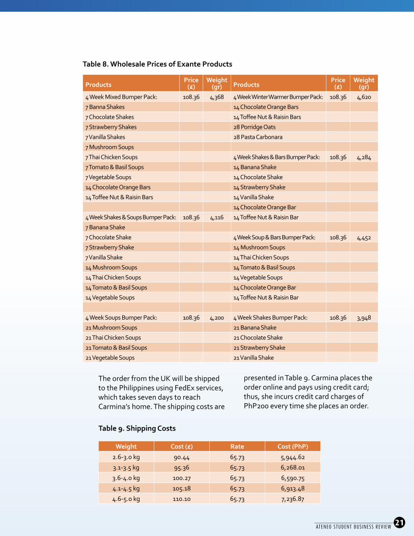
Table 8. Wholesale Prices of Exante Products

The order from the UK will be shipped to the Philippines using FedEx services, which takes seven days to reach Carmina’s home. The shipping costs are

presented in Table 9. Carmina places the order online and pays using credit card; thus, she incurs credit card charges of PhP200 every time she places an order.

Table 9. Shipping Costs

ProductsPrice (£)

Weight (gr) Products

Price (£)

Weight (gr)

Diet Shakes Diet Soups

Banana Shake 2.58 47 Mushroom Soups 2.58 48

Chocolate Shake 2.58 48 Thai Chicken Soups 2.58 48

Strawberry Shake 2.58 47 Tomato & Basil Soups 2.58 53

Vanilla Shake 2.58 46 Vegetable Soups 2.58 51

Box of 50 Banana Shakes 64.50 2,500 Box of 50 Mushroom Soups 64.50 2,550

Box of 50 Chocolate Shakes 64.50 2,500 Box of 50 Thai Chicken Soups 64.50 2,600

Box of 50 Strawberry Shakes 64.50 2,500 Box of 50 Tomato & Basil Soups 64.50 2,650

Box of 50 Vanilla Shakes 64.50 2,500 Box of 50 Vegetable Soups 64.50 2,550

Diet Bars Food Packs

Chocolate Orange Bar 2.58 59 Porridge Oats 2.58 53

Toffee Nut & Raisin Bar 2.58 59 Pasta Carbonara 2.58 53

Box of 50 Chocolate Orange Bars 64.50 2,950 Box of 50 Porridge Oats 64.50 2,650

Box of 50 Toffee Nut & Raisin Bars 64.50 2,950 Box of 50 Pasta Carbonara 64.50 2,650

ProductsPrice

(£)Weight

(gr) ProductsPrice

(£)Weight

(gr)4 Week Mixed Bumper Pack: 108.36 4,368 4 Week Winter Warmer Bumper Pack: 108.36 4,620

7 Banna Shakes 14 Chocolate Orange Bars

7 Chocolate Shakes 14 Toffee Nut & Raisin Bars

7 Strawberry Shakes 28 Porridge Oats

7 Vanilla Shakes 28 Pasta Carbonara

7 Mushroom Soups

7 Thai Chicken Soups 4 Week Shakes & Bars Bumper Pack: 108.36 4,284

7 Tomato & Basil Soups 14 Banana Shake

7 Vegetable Soups 14 Chocolate Shake

14 Chocolate Orange Bars 14 Strawberry Shake

14 Toffee Nut & Raisin Bars 14 Vanilla Shake

14 Chocolate Orange Bar

4 Week Shakes & Soups Bumper Pack: 108.36 4,116 14 Toffee Nut & Raisin Bar

7 Banana Shake

7 Chocolate Shake 4 Week Soup & Bars Bumper Pack: 108.36 4,452

7 Strawberry Shake 14 Mushroom Soups

7 Vanilla Shake 14 Thai Chicken Soups

14 Mushroom Soups 14 Tomato & Basil Soups

14 Thai Chicken Soups 14 Vegetable Soups

14 Tomato & Basil Soups 14 Chocolate Orange Bar

14 Vegetable Soups 14 Toffee Nut & Raisin Bar

4 Week Soups Bumper Pack: 108.36 4,200 4 Week Shakes Bumper Pack: 108.36 3,948

21 Mushroom Soups 21 Banana Shake

21 Thai Chicken Soups 21 Chocolate Shake

21 Tomato & Basil Soups 21 Strawberry Shake

21 Vegetable Soups 21 Vanilla Shake

Weight Cost (£) Rate Cost (PhP)

2.6-3.0 kg 90.44 65.73 5,944.62

3.1-3.5 kg 95.36 65.73 6,268.01

3.6-4.0 kg 100.27 65.73 6,590.75

4.1-4.5 kg 105.18 65.73 6,913.48

4.6-5.0 kg 110.10 65.73 7,236.87


Carmina wants to know the optimal quantity for ordering the Exante Diet products. Should Carmina consider buying the Bumper Packs given the lower price?

Applying the economic order quantity (EOQ) approach, the given variables are as follows: The Annual Demand is 1,092 units of a single product (based on 52 weeks, 7 days, and 3 single products/day), the Ordering Cost is PhP200, and the Carrying Cost is the Cost of Capital (assume 10%) applied on the Product Unit Cost. To fulfill the lightest weight in determining Shipping Cost (0.10 kg), two pieces of a single Product are used for comparison instead of one piece of a single Product because one piece weight

is only 0.05 kg, whereas the total weight of two pieces is 0.10 kg.

Following the EOQ computations shown in Table 10, the optimal order quantity of Exante Diet products for Carmina is as follows:

• If she decides to buy two pieces of any single product, the EOQ is 23 units of 2 pieces of any single product.

• If she decides to buy any Box of 50, the EOQ is 3 units of any Box of 50.

• If she decides to buy any of 4-week Bumper Packs, the EOQ is 2 units of any 4-week Bumper Packs.

Table 10. EOQ Computation for Each Package of Products

2 Pieces of a Single

Product

Box of 50 Diet Shakes

Box of 50 Diet Bars

Box of 50 Diet Soups Box of 50

Food Packs

Unit Cost (in £) 5.16 64.5 64.5 64.5 64.5

Exchange Rate 65.73 65.73 65.73 65.73 65.73

Unit Cost (in PhP) 339.17 4,239.59 4,239.59 4,239.59 4,239.59

Product Weight (in kg) 0.1 2.5 2.95 2.59 2.65

Shipping Cost (in PhP) 3,930 5,622 5,945 5,945 5,945

Cost of Capital 10% 10% 10% 10% 10%

Cost to Carry (PhP) 427 986 1,018 1,018 1,018

Cost per Order (PhP) 200 200 200 200 200

Annual Demand (D) 546 22 22 22 22

EOQ 23 3 3 3 3


Table 10 continuation

Given the Total Annual Cost of each option as presented in Table 11, the best option is the 4-week Shakes Bumper Pack, which results in the lowest total annual cost compared to other options. However, if Carmina prefers variety in her diet meals, she can buy the second

lowest cost options, namely, 4-Week Mixed Bumper Pack, 4-Week Shakes and Bars Bumper Pack, 4-Week Shakes and Soups Bumper Pack, or 4-Week Soups and Bars Bumper Pack, each pack containing different meals.

Table 11. Comparison of Costs

Total Product

Cost

Total Ordering

Cost

Total Carrying

Cost

Total Annual Costs

2 Pieces of a Single Product 2,330,963 4,828 4,828 2,340,619

Box of 50 Diet Shakes 215,375 1,468 1,468 218,310

Box of 50 Diet Bars 222,423 1,491 1,491 225,406

Box of 50 Diet Soups 222,423 1,491 1,491 225,406

Box of 50 Food Packs 222,423 1,491 1,491 225,406

4-Week Mixed Bumper Pack 182,468 1,351 1,351 185,169

4-Week Winter Warmer Bumper Pack 186,672 1,366 1,366 189,404

4-Week Shakes and Bars Bumper Pack 182,468 1,351 1,351 185,169

4-Week Shakes and Soups Bumper Pack 182,468 1,351 1,351 185,169

4-Week Soups and Bars Bumper Pack 182,468 1,351 1,351 185,169

4-Week Soups Bumper Pack 182,468 1,351 1,351 185,169

4-Week Shakes Bumper Pack 178,272 1,335 1,335 180,943

4-Week Mixed

Bumper Pack

4-Week Winter

Warmer Bumper

Pack

4-Week Shakes & Bars

Bumper Pack

4-Week Shakes

& Soups Bumper

Pack

4-Week Soups & Bars

Bumper Pack

4-Week Soups

Bumper Pack

4-Week Shakes Bumper

Pack

Unit Cost (in £) 108.36 108.36 108.36 108.36 108.36 108.36 108.36

Exchange Rate 65.73 65.73 65.73 65.73 65.73 65.73 65.73

Unit Cost (in PHP) 7,122.50 7,122.50 7,122.50 7,122.50 7,122.50 7,122.50 7,122.50

Products weight (in kg) 4.37 4.62 4.28 4.12 4.45 4.2 3.95

Shipping Cost (in PhP) 6,913 7,237 6,913 6,913 6,913 6,913 6,591

Cost of Capital 10% 10% 10% 10% 10% 10% 10%

Cost to Carry (PhP) 1,404 1,436 1,404 1,404 1,404 1,404 1,371

Cost per Order (PhP) 200 200 200 200 200 200 200

Annual Demand (D) 13 13 13 13 13 13 13

EOQ 2 2 2 2 2 2 2


Queuing Theory: Business on the Side

Carmina Florentino-Reyes is greatly amazed at the highly practical applications of quantitative methods in her daily routine as a mother and as a woman.

Now, Carmina wants to know how such methods can help her to improve the operations of her family-owned business, CFR DIAL-A-MASSAGE, which she continuously manages even after giving birth to the triplets. She intends to apply the concepts of Queuing Theory to determine the average time that a caller must wait before reaching the reservation staff, the average number of calls waiting to be connected to the reservation staff, and the average time for a caller to complete a call (i.e., waiting time plus service time).

CFR DIAL-A-MASSAGE has one female reservation staff on duty at a time. She handles information about the schedules of available therapists and makes reservation. All calls to CFR DIAL-A-MASSAGE are answered by a voice messaging system. If the reservation staff is available, the call is transferred to her. If she is busy, the caller is put on hold. When the reservation staff becomes available, the voice messaging system transfers the caller who has been waiting the longest.

Assume that arrivals follow a Markov process (inter-arrival times are exponential) with an average inter-arrival time of six minutes. Reservation staff takes an average of four minutes to service a customer, and the standard deviation for this service time is two minutes.

The following aspects are determined: (1) the average time that a caller must wait before reaching a reservation staff; (2) the average number of calls waiting to be connected to a reservation staff; and (3) the average time for a caller to complete a call (i.e., waiting time plus service time).

By applying the concepts of Queuing Theory, the performance metrics of the system are measured. This framework is an M/G/1 queue model in which the mean interarrival time (μa) = 6, the mean service time (µs) = 4, and the standard deviation (SD) = 2. The following variables are computed:

Coefficient of variation of service time (cvs) = SD/ µs = 2/4 = 0.5

System utilization (r) = µs/µa = 4/6 = 0.667

Waiting time multiple (WTM) = ((r/(1-r))((1+cvs2)/2) = 1.25Therefore, Mean waiting time (µw) = (µs) (WTM) = 4×1.25 = 5 minutes

Mean line length (µL) = µw/µa = 5/6 = 0.83 person

Mean time in system = µw + µs = 5 + 4 = 9 minutes

The average time that a caller must wait before reaching the reservation staff is five minutes. The average number of calls waiting to be connected to the reservation staff is 0.83, and the average time for a caller to complete a call (i.e. waiting time plus service time) is nine minutes.


Monte Carlo Simulation: Eggs Dilemma

In the middle of her busy daily schedule—taking care of the new babies, her three-year-old daughter, and her husband, as well as her massage business—Carmina also has to look after the daily needs of her family. Part of her responsibility is ensuring the availability of eggs inside her refrigerator. Eggs are rich sources of protein and vitamin D; they contain 11 different vitamins and minerals that are essential for health.

After reaping the benefits of quantitative concepts in four separate endeavors, Carmina opted to apply another quantitative method to even the simplest problem. Carmina acknowledged that her family does not consume the same quantity of eggs every day; thus, she decided to employ the Monte Carlo simulation method. Table 12 presents the family’s egg consumption for the past 100 days.

To save time, Carmina prefers to order the eggs from a grocery store, which takes two days for the delivery. When Carmina finds that only five eggs are left in the refrigerator, she will call the store and order the eggs. Each pack contains one dozen eggs.

Carmina wants to determine the schedule for ordering eggs and manage their inventory ensure the constant availability of eggs at home.

From the past three-month data of egg consumption of her family, Carmina attempts to figure out their egg consumption for the next three months, hence allowing her to determine the schedule for ordering eggs and manage their inventory.

The three-month simulation is performed in Table 13. The simulation predicted that the family will consume 157 eggs in the next 90 days. Running the simulation at different reorder points (i.e., the level of inventory that triggers Carmina to reorder) is easy. Different reorder points generate different inventory scenarios as shown in Table 14. The reorder point of 7 assures the availability of eggs for Carmina’s family to consume anytime they want.

Table 12. Historical Egg Consumption

Egg Consumption

DaysOccurred

RelativeFrequency

RandomNumbersAssigned

0 15 15% 00 to 14

1 23 23% 15 to 37

2 29 29% 38 to 66

3 12 12% 67 to 78

4 12 12% 79 to 90

5 9 9% 91 to 99

100


Table 14. Simulated Reorder Points

Reorder Point Minimum Inventory

Maximum Inventory

Average Inventory

4 -2 16 8

5 0 16 9

6 0 18 9

7 3 18 10

8 3 18 11

9 3 19 11

Day Receipts BeginningInventory Random Number Consumption Ending

Inventory Buying

1 12 29 1 11 0

2 11 10 0 11 0

3 0 11 81 4 7 12

4 0 7 81 4 3 0

5 12 3 7 0 15 0

6 0 15 37 1 14 0

7 0 14 90 4 10 0

8 0 10 2 0 10 0

9 0 10 25 1 9 0

10 0 9 13 0 9 0

11 0 9 91 5 4 12

12 0 4 2 0 4 0

13 12 4 87 4 12 0

14 0 12 17 1 11 0

15 0 11 96 5 6 12

16 0 6 5 0 6 0

17 12 6 5 0 18 0

18 0 18 34 1 17 0

19 0 17 59 2 15 0

20 0 15 62 2 13 0

21 0 13 17 1 12 0

22 0 12 66 2 10 0

23 0 10 44 2 8 0

24 0 8 26 1 7 12

25 0 7 78 3 4 0

26 12 4 46 2 14 0

27 0 14 7 0 14 0

28 0 14 7 0 14 0

29 0 14 57 2 12 0

30 0 12 65 2 10 0

31 0 10 91 5 5 12

32 0 5 9 0 5 0

33 12 5 45 2 15 0

34 0 15 0 0 15 0

35 0 15 29 1 14 0

36 0 14 66 2 12 0

37 0 12 78 3 9 0

38 0 9 27 1 8 0

Table 13. Three-Month Egg Simulation


Day Receipts Beginning Inventory Random Number Consumption Ending

Inventory Buying

39 0 8 36 1 7 12

40 0 7 32 1 6 0

41 12 6 38 2 16 0

42 0 16 60 2 14 0

43 0 14 15 1 13 0

44 0 13 63 2 11 0

45 0 11 92 5 6 12

46 0 6 39 2 4 0

47 12 4 26 1 15 0

48 0 15 81 4 11 0

49 0 11 89 4 7 12

50 0 7 89 4 3 0

51 12 3 34 1 14 0

52 0 14 72 3 11 0

53 0 11 0 0 11 0

54 0 11 84 4 7 12

55 0 7 53 2 5 0

56 12 5 22 1 16 0

57 0 16 64 2 14 0

58 0 14 33 1 13 0

59 0 13 28 1 12 0

60 0 12 41 2 10 0

61 0 10 70 3 7 12

62 0 7 71 3 4 0

63 12 4 75 3 13 0

64 0 13 20 1 12 0

65 0 12 7 0 12 0

66 0 12 66 2 10 0

67 0 10 12 0 10 0

68 0 10 22 1 9 0

69 0 9 51 2 7 12

70 0 7 60 2 5 0

71 12 5 97 5 12 0

72 0 12 49 2 10 0

73 0 10 95 5 5 12

74 0 5 16 1 4 0

75 12 4 3 0 16 0

76 0 16 43 2 14 0

77 0 14 8 0 14 0

78 0 14 20 1 13 0

79 0 13 51 2 11 0

80 0 11 47 2 9 0

81 0 9 7 0 9 0

82 0 9 89 4 5 12

83 0 5 35 1 4 0

84 12 4 10 0 16 0

85 0 16 11 0 16 0

86 0 16 16 1 15 0

87 0 15 37 1 14 0

88 0 14 20 1 13 0

89 0 13 8 0 13 0

90 0 13 64 2 11 0


SAP Systems Implementations:

OptimizingProject Staffing

through LinearProgramming

Evan W. Yeung


Products and Services

lectronic System Infrastructure (ESI) Consulting Philippines Inc. offers application services and platform and infrastructure services that cater to the needs of both

consumers and enterprises. A list of services currently offered by the company follows:

• Application services

• Business process outsourcing

• Cloud services

• Consulting services: Converged infrastructure

• Consulting services: IT transformation

• IT infrastructure outsourcing

• Services by product

• Software services

• Software support

With such services, majority of the company’s clients are evidently top-tier corporations. The costs of maintaining the real seamless integration of technology into the business, as well as the end-to-end approach to implementation, improvement, and support are high; thus, small business are highly unlikely to embrace these concepts. In this context, ESI Consulting has begun developing smaller business applications such as cloud services to tap the market of small to mid-

size enterprises. Although the technology is still in its infancy and the value it brings is yet to be truly understood, the company continues to prioritize large enterprises as its main profit drivers.

Consulting Services: SAP Systems

The business model for ESI Consulting comprises a wide array of technological services offered to both consumers and corporate clients. This paper focuses on the project-based business models of ESI Consulting, specifically SAP (Systems, Applications, Products in Data Processing) Enterprise Systems implementations for large corporations.

The partnership between ESI Consulting and SAP AG has led to an unprecedented success in creating enterprise systems for other businesses. The success of SAP systems was mainly due to their flexibility to be configured and engineered to adapt to any business setting. However, implementing such systems for companies that are not adept in the concept of information technology can be complex and tedious. Against this background, SAP together with several of its partners (including ESI Consulting) created a new way of conducting business: offering corporate clients, for a price, the expertise of trained professionals in implementing such systems. The “SAP Practice” was developed through this approach.

The success of SAP systems was mainly due to their flexibility to be configured and engineered to adapt to any business setting.

E


Standard SAP Project Methodology

As an increasing number of companies implement Enterprise Resource Planning (ERP) Systems, developing a methodology or a process of implementing such systems is a rational step for companies selling ERP systems. With SAP as the forefront of such technology, the company developed a methodology for a more streamlined project implementation. This methodology is called the “Accelerated-SAP” (ASAP) roadmap. As illustrated in Figure 1, the

roadmap shows the key phases of a standard SAP implementation project. The roadmap provides management with a bird’s eye view of the steps to be taken, as well as the life cycle of creating a system that fits client needs. The end result is that the ASAP roadmap delivers tremendous benefits, such as faster and more efficient use of resources and reduced cost for an effective project management standard.

SAP Practice Services

The current systems in which ESI Consulting operates its SAP practice business engage highly trained individuals in the aspect of SAP process and deploy them to clients worldwide. Thus, the ASAP methodology is employed to carry out the implementations. However, given the high demand for SAP and the increase in consulting services in the Philippines at an unprecedented rate, the SAP practice team of ESI Consulting requires efficient staffing techniques to ensure high quality of service.

The company currently holds several accounts worldwide. With an increasing number of projects being routed to the Philippines due to its low-cost labor, the ESI Consulting management team is required to effectively staff forthcoming projects with the most qualified individuals. As clients come from North America and Latin America (NALA), Europe Middle East and Africa (EMEA), and Asia Pacific (AP), staffing SAP experts can be complex. To add more complexity, each module of the SAP system is specific to an individual, and the requirements of each client are unique. This factor requires the company to adopt a stringent process not only in project implementation itself, but also in the way the project team is assembled.

Figure 2 shows the core business processes that can be implemented in an SAP system. Although not all processes are needed in every business, the key modules that are always present in a project implementation are Sales & Distribution, Materials

1

2 34 5Project

PreparationBusinessBlueprint

RealizationFinal

Preparation Go Live &Support

• Project Management• Organizational Change Management• Training• Develop System Environment• Organizational Structure Definition• Business Process Analysis• Business Process Definition• Quality Check

• Project Management• Training• System Management• Detailed Project Planning• Cutover• Quality Check

Continuous

Improvement

• Production Support• Project End

• Initial Project Planning• Project Procedures• Training• Project Kickoff• Technical Requirements• Quality Check

• Project Management• Organizational Change Management• Training• Baseline Configuration and Confirmation• System Management• Final Configuration and Confirmation• Develop Programs, Interfaces etc.• Final Integration Test• Quality Check

Defining the Points on the ASAP Roadmap

Figure 1. Standard SAP Methodology


Management, Production Planning (only for Manufacturing Businesses), Financial Accounting, and Controlling. This paper focuses on these modules as part of its scope in using Management Science techniques to improve the staffing process.

Objective

This paper aims to employ the concepts of linear programming in the complex project staffing needed by ESI Consulting SAP Practice team for SAP implementations. The paper is written in the context of a Delivery Manager, who is mainly responsible for coordinating with the clients the assembly a project team for engagement. With project demands

at an all-time high, and clients coming in from offshore locations where onsite consulting are needed, employing linear programming model should streamline the process for better results. The goal of the Delivery Manager is to maximize profit by optimizing the usage of SAP experts in the organization.

Research Data

This paper uses approximate data, such as pricing and margins for each consultant. The pricing for a full-time equivalent (FTE) varies with the experience level of the consultant and the region in which the client is located. The profits to be generated are based solely on the number of consultants engaged from the Philippine office. For any unstaffed project needed, the company would look elsewhere to ensure that the proper project team is assembled (e.g., Regional Headquarters in India and/or Singapore).

Table 1 presents the approximate average pricing and salary of each consultant level for each region, from which the profit margin generated per full-time equivalent engaged per month can be estimated. Furthermore, the assumption is that the clients will shoulder most expenses incurred, such as the travel expenditures of the consultants and the project manager.

With project demands at an all-time high, and clients coming in from offshore locations where onsite consulting are needed, employing linear programming model should streamline the process for better results.

FISD

ISHR

Client/Server

R/3

COMM

WFPM

AMPP

PSQM

R/3 Core Business Process

FinancialAccounting

Controlling

Fixed AssetManagement

Project System

Workflow

IndustrySolutions

Sales &Distribution

MaterialManagement

ProductionPlanning

QualityManagement

PlantMaintenance

HumanResources

Figure 2. SAP Modules and Core Processes


Table 1. Pricing for SAP Consulting Services (in US$/month)

The number of consultants needed for a project team will vary depending on the requirements of the clients. However, a project manager should be assigned to each project.

Table 2 shows the number of employees per core process working

for the company’s SAP practice delivery team. The number of project managers available is also listed in the table. The consultant levels provide information on how the Delivery Manager will staff the project based on its complexity.

Table 2. Staff Count

Core Process/SAP Module Consultant Level Number of Employees FTESAP Financial Accounting Entry-Level (Junior) 42 42

Intermediate 20 40

Senior 7 21

SAP Controlling Entry-Level (Junior) 40 40

Intermediate 30 60

Senior 10 30

SAP Sales & Distribution Entry-Level (Junior) 23 23

Intermediate 16 32

Senior 10 30

SAP Materials Management Entry-Level (Junior 42 42

Intermediate 28 56

Senior 14 42

SAP Production Planning Entry-Level (Junior) 21 21

Intermediate 10 20

Senior 5 15

Total 318 514

Region Consultant Level Ave. Pricing Ave. Salary MarginAmericas (NALA) Entry-Level (Junior) 2,000 625 1,375

Intermediate 3,800 1,500 2,300

Senior 7,500 2,500 5,000

Project Manager 7,800 2,800 5,000

Europe, Middle East & Africa (EMEA) Entry-Level (Junior) 2,000 625 1,375


Senior 6,800 2,500 4,300


Asia Pacific (AP) Entry-Level (Junior) 1,500 625 875


Senior 5,500 2,500 3,000



Table 3 shows the FTE demand for a specific project type, and Table 4 shows the FTE allocation of each position. This information should allow the Delivery

Manager to determine the compensation based on the consultant level to be assigned to a specific project type.

Table 3. Project Data

Consultant Level Full-Time Equivalent

Entry-Level (Junior) 1

Intermediate 2

Senior 3

Table 4. Equivalent FTE

Project Type Core Process FTE Demand per Project

Large(Complex and High Budget)

Financial Accounting 7

Controlling 8

Sales & Distribution 4

Materials Management 9

Production Planning 3

Medium(Moderate Complexity)


Controlling 6




Small(Average and Low Budget)


Controlling 4





Table 5. Forecasted Projects

Model for Linear Programming

Decision Variables

NALA1-FI Number of Entry-Level Consultants Assigned to NALA Projects for Financial Accounting

NALA1-CO Number of Entry-Level Consultants Assigned to NALA Projects for Controlling

NALA1-SD Number of Entry-Level Consultants Assigned to NALA Projects for Sales & Distribution

NALA1-MM Number of Entry-Level Consultants Assigned to NALA Projects for Materials Management

NALA1-PP Number of Entry-Level Consultants Assigned to NALA Projects for Production Planning

NALA2-FI Number of Intermediate Consultants Assigned to NALA Projects for Financial Accounting

NALA2-CO Number of Intermediate Consultants Assigned to NALA Projects for Controlling

NALA2-SD Number of Intermediate Consultants Assigned to NALA Projects for Sales & Distribution

NALA2-MM Number of Intermediate Consultants Assigned to NALA Projects for Materials Management

NALA2-PP Number of Intermediate Consultants Assigned to NALA Projects for Production Planning

NALA3-FI Number of Senior Consultants Assigned to NALA Projects for Financial Accounting

NALA3-CO Number of Senior Consultants Assigned to NALA Projects for Controlling

NALA3-SD Number of Senior Consultants Assigned to NALA Projects for Sales & Distribution

NALA3-MM Number of Senior Consultants Assigned to NALA Projects for Materials Management

NALA3-PP Number of Senior Consultants Assigned to NALA Projects for Production Planning

EMEA1-FI Number of Entry-Level Consultants Assigned to EMEA Projects for Financial Accounting

EMEA1-CO Number of Entry-Level Consultants Assigned to EMEA Projects for Controlling

EMEA1-SD Number of Entry-Level Consultants Assigned to EMEA Projects for Sales & Distribution

EMEA1-MM Number of Entry-Level Consultants Assigned to EMEA Projects for Materials Management

EMEA1-PP Number of Entry-Level Consultants Assigned to EMEA Projects for Production Planning

EMEA2-FI Number of Intermediate Consultants Assigned to EMEA Projects for Financial Accounting

EMEA2-CO Number of Intermediate Consultants Assigned to EMEA Projects for Controlling

Table 5 presents the information on forthcoming projects based on forecasted demand. A total of 22 projects

will be available. This data is used for calculation purposes in the linear programming model.

Project Type Region Number of Projects

Large NALA 1

EMEA 2

AP 1

Medium NALA 2

EMEA 5

AP 3

Small NALA 2

EMEA 1

AP 5


EMEA2-SD Number of Intermediate Consultants Assigned to EMEA Projects for Sales & Distribution

EMEA2-MM Number of Intermediate Consultants Assigned to EMEA Projects for Materials Management

EMEA2-PP Number of Intermediate Consultants Assigned to EMEA Projects for Production Planning

EMEA3-FI Number of Senior Consultants Assigned to EMEA Projects for Financial Accounting

EMEA3-CO Number of Senior Consultants Assigned to EMEA Projects for Controlling

EMEA3-SD Number of Senior Consultants Assigned to EMEA Projects for Sales & Distribution

EMEA3-MM Number of Senior Consultants Assigned to EMEA Projects for Materials Management

EMEA3-PP Number of Senior Consultants Assigned to EMEA Projects for Production Planning

AP1-FI Number of Entry-Level Consultants Assigned to AP Projects for Financial Accounting

AP1-CO Number of Entry-Level Consultants Assigned to AP Projects for Controlling

AP1-SD Number of Entry-Level Consultants Assigned to AP Projects for Sales & Distribution

AP1-MM Number of Entry-Level Consultants Assigned to AP Projects for Materials Management

AP1-PP Number of Entry-Level Consultants Assigned to AP Projects for Production Planning

AP2-FI Number of Intermediate Consultants Assigned to AP Projects for Financial Accounting

AP2-CO Number of Intermediate Consultants Assigned to AP Projects for Controlling

AP2-SD Number of Intermediate Consultants Assigned to AP Projects for Sales & Distribution

AP2-MM Number of Intermediate Consultants Assigned to AP Projects for Materials Management

AP2-PP Number of Intermediate Consultants Assigned to AP Projects for Production Planning

AP3-FI Number of Senior Consultants Assigned to AP Projects for Financial Accounting

AP3-CO Number of Senior Consultants Assigned to AP Projects for Controlling

AP3-SD Number of Senior Consultants Assigned to AP Projects for Sales & Distribution

AP3-MM Number of Senior Consultants Assigned to AP Projects for Materials Management

AP3-PP Number of Senior Consultants Assigned to AP Projects for Production Planning

Decision Variables

Objective: Profit = Revenues - Cost

!

Maximize Profit = [1,375 (NALA1FI + NALA1CO + NALA1SD + NALA1MM + NALA1PP) + 2,300 (NALA2FI + NALA2CO + NALA2SD + NALA2MM + NALA2PP) + 5,000 (NALA3FI + NALA3CO + NALA3SD + NALA3MM + NALA3PP) + 1,375 (EMEA1FI + EMEA1CO + EMEA1SD + EMEA1MM + EMEA1PP) + 2,100 (EMEA2FI + EMEA2CO + EMEA2SD + EMEA2MM + EMEA2PP) + 4,300 (EMEA3FI + EMEA3CO + EMEA3SD + EMEA3MM + EMEA3PP) + 875 (AP1FI + AP1CO + AP1SD + AP1MM + AP1PP) + 1,300 (AP2FI + AP2CO + AP2SD + AP2MM + AP2PP) + 3,000 (AP3FI + AP3CO + AP3SD + AP3MM + AP3PP)]

This objective shows the computation based on the margin of each region specific to a consultant level.


Constraints

1. FTE Demand

2. Supply Constraints

FI: NALA1FI + 2(NALA2FI) + 3(NALA3FI) >= 23EMEA1FI + 2(EMEA2FI) + 3(EMEA3FI) >= 42AP1FI + 2(AP2FI) + 3(AP3FI) >= 37

CO: NALA1CO + 2(NALA2CO) + 3(NALA3CO) >= 28EMEA1CO + 2(EMEA2CO) + 3(EMEA3CO) >= 50AP1CO + 2(AP2CO) + 3(AP3CO) >= 46

SD: NALA1SD + 2(NALA2SD) + 3(NALA3SD) >= 12EMEA1SD + 2(EMEA2SD) + 3(EMEA3SD) >= 20AP1SD + 2(AP2SD) + 3(AP3SD) >= 20

MM: NALA1MM + 2(NALA2MM) + 3(NALA3MM) >= 31EMEA1MM + 2(EMEA2MM) + 3(EMEA3MM) >= 57AP1MM + 2(AP2MM) + 3(AP3MM) >= 50

PP: NALA1PP + 2(NALA2PP) + 3(NALA3PP) >= 5EMEA1PP + 2(EMEA2PP) + 3(EMEA3PP) >= 11AP1PP + 2(AP2PP) + 3(AP3PP) >= 6

FI1: NALA1FI + EMEA1FI + AP1FI <= 42



CO1: NALA1CO + EMEA1CO + AP1CO <= 40



SD1: NALA1SD + EMEA1SD + AP1SD <= 23



MM1: NALA1MM + EMEA1MM + AP1MM <= 42



PP1: NALA1PP + EMEA1PP + AP1PP <= 21




3. Integer Constraints

All variables should be an integer value.

Solution

Refer to the Solver Template for the optimization solution. The optimal distribution of the consultants is shown in Table 6. Total profit of this optimal distribution is $616,800.

Table 6. Optimal Distribution

Conclusion

The staffing and project engagements of ESI Consulting SAP practice team can be optimized through linear programming. The complexity of the process can be quite tedious; nevertheless, in terms of staffing appropriate consultants to ensure high quality of output and service and thereby generate profits for the company, linear programming may prove to be the most suitable model for this type of setup.

References “Accelerated SAP (ASAP) Methodology” SAP Materials Management, retrieved from http://sapmmstudy.blogspot.com/2012/08/asap-methodology.html on Nov. 11, 2012.

2Santosh Kumar, “Different Modules in SAP” SAP Mentors, retrieved from http://abapmentors.blogspot.com/2012/04/different-modules-in-sap.html on Nov. 11, 2012

NALA EMEA AP Count FTEs

Financial Accounting Entry-Level 41 1 42 42

Intermediate 1 1 18 20 40

Senior 7 7 21

Controlling Entry-Level 40 40 40

Intermediate 2 5 23 30 60

Senior 10 10 30

Sales & Distribution Entry-Level 1 20 2 23 23

Intermediate 7 9 16 32

Senior 10 10 30

Materials Management Entry-Level 42 42 42

Intermediate 3 25 28 56

Senior 11 3 14 42

Production Planning Entry-Level 4 11 6 21 21

Intermediate 10 10 20

Senior 5 5 15

Total 68 166 84 318 514


Pro

blem

Obj

ecti

ve 12

34

56

78

910

1112

1314

1516

1718

1920

2122

23

Dec

isio

n V

aria

ble

IDN

ALA

1FI

NA

LA2F

IN

ALA

3FI

NA

LA1C

ON

ALA

2CO

NA

LA3C

ON

ALA

1SD

NA

LA2S

DN

ALA

3SD

NA

LA1M

MN

ALA

2MM

NA

LA3M

MN

ALA

1PP

NA

LA2P

PN

ALA

3PP

EMEA

1FI

EMEA

2FI

EMEA

3FI

EMEA

1CO

EMEA

2CO

EMEA

3CO

EMEA

1SD

EMEA

2SD

Qua

ntity

(lea

ve b

lank

)0

17

02

101

710

00

114

105

411

040

50

200

Uni

t coe

ffici

ents

1375

2300

5000

1375

2300

5000

1375

2300

5000

1375

2300

5000

1375

2300

5000

1375

2100

4300

1375

2100

4300

1375

2100

Tota

l Obj

ectiv

e0

2300

3500

00

4600

5000

013

7516

100

5000

00

055

000

5500

2300

025

000

5637

521

000

5500

010

500

027

500

0

Cons

trai

nt C

oeffi

cien

ts

DEM

AND

FI at

NAL

A1

23

DEM

AND

CO

at N

ALA

12

3

DEM

AND

SD

at N

ALA

12

3

DEM

AND

MM

at N

ALA

12

3

DEM

AND

PP

at N

ALA

12

3

DEM

AND

FI at

EM

EA1

23

DEM

AND

CO

at E

MEA

12

3

DEM

AND

SD

at E

MEA

12

DEM

AND

MM

at E

MEA

DEM

AND

PP

at E

MEA

DEM

AND

FI at

AP

DEM

AND

CO

at A

P

DEM

AND

SD

at A

P

DEM

AND

MM

at A

P

DEM

AND

PP

at A

P

SUPP

LY FI

11

1

SUPP

LY FI

21

1

SUPP

LY FI

31

1

SUPP

LY C

O1

11

SUPP

LY C

O2

11

SUPP

LY C

O3

11

SUPP

LY S

D1

11

SUPP

LY S

D2

11

SUPP

LY S

D3

1

SUPP

LY M

M1

1

SUPP

LY M

M2

1

SUPP

LY M

M3

1

SUPP

LY P

P11

SUPP

LY P

P21

SUPP

LY P

P31

SOLV

ER T

EMP

LATE

Cas

e P

robl

em N

ame:

SA

P S

yste

ms

Impl

emen

tati

ons


Pro

blem

Obj

ecti

veTo

tal

Obj

ecti

ve24

2526

2728

2930

3132

3334

3536

3738

3940

4142

4344

45

Dec

isio

n V

aria

ble

IDEM

EA3S

DEM

EA1M

MEM

EA2M

MEM

EA3M

MEM

EA1P

PEM

EA2P

PEM

EA3P

PAP

1FI

AP2F

IAP

3FI

AP1C

OAP

2CO

AP3C

OAP

1SD

AP2S

DAP

3SD

AP1M

MAP

2MM

AP3M

MAP

1PP

AP2P

PAP

3PP

Qua

ntity

(lea

ve b

lank

)0

423

311

00

118

00

230

29

00

250

60

0

Uni

t coe

ffici

ents

4300

1375

2100

4300

1375

2100

4300

875

1300

3000

875

1300

3000

875

1300

3000

875

1300

3000

875

1300

3000

Tota

l Obj

ectiv

e0

5775

063

0012

900

1512

50

087

523

400

00

2990

00

1750

1170

00

032

500

052

500

061

6800

Cons

trai

nt C

oeffi

cien

ts

DEM

AND

FI at

NAL

A

DEM

AND

CO

at N

ALA

DEM

AND

SD

at N

ALA

DEM

AND

MM

at N

ALA

DEM

AND

PP

at N

ALA

DEM

AND

FI at

EM

EA

DEM

AND

CO

at E

MEA

DEM

AND

SD

at E

MEA

3

DEM

AND

MM

at E

MEA

12

3

DEM

AND

PP

at E

MEA

12

3

DEM

AND

FI at

AP

12

3

DEM

AND

CO

at A

P1

23

DEM

AND

SD

at A

P1

23

DEM

AND

MM

at A

P1

23

DEM

AND

PP

at A

P1

23

SUPP

LY FI

11

SUPP

LY FI

21

SUPP

LY FI

31

SUPP

LY C

O1

1

SUPP

LY C

O2

1

SUPP

LY C

O3

1

SUPP

LY S

D1

1

SUPP

LY S

D2

1

SUPP

LY S

D3

11

SUPP

LY M

M1

11

SUPP

LY M

M2

11

SUPP

LY M

M3

11

SUPP

LY P

P11

1

SUPP

LY P

P21

1

SUPP

LY P

P31

1

SOLV

ER T

EMP

LATE

Cas

e P

robl

em N

ame:

SA

P S

yste

ms

Impl

emen

tati

ons


Pro

blem

Obj

ecti

ve 12

34

56

78

910

1112

1314

1516

1718

1920

2122

23

Dec

isio

n V

aria

ble

IDN

ALA

1FI

NA

LA2F

IN

ALA

3FI

NA

LA1C

ON

ALA

2CO

NA

LA3C

ON

ALA

1SD

NA

LA2S

DN

ALA

3SD

NA

LA1M

MN

ALA

2MM

NA

LA3M

MN

ALA

1PP

NA

LA2P

PN

ALA

3PP

EMEA

1FI

EMEA

2FI

EMEA

3FI

EMEA

1CO

EMEA

2CO

EMEA

3CO

EMEA

1SD

EMEA

2SD

Qua

ntity

(lea

ve b

lank

)0

17

02

101

710

00

114

105

411

040

50

200

Uni

t coe

ffici

ents

1375

2300

5000

1375

2300

5000

1375

2300

5000

1375

2300

5000

1375

2300

5000

1375

2100

4300

1375

2100

4300

1375

2100

Tota

l Obj

ectiv

e0

2300

3500

00

4600

5000

013

7516

100

5000

00

055

000

5500

2300

025

000

5637

521

000

5500

010

500

027

500

0

Cons

trai

nt R

esul

ts

DEM

AND

FI at

NAL

A0

221

00

00

00

00

00

00

00

00

00

00

DEM

AND

CO

at N

ALA

00

00

430

00

00

00

00

00

00

00

00

0

DEM

AND

SD

at N

ALA

00

00

00

114

300

00

00

00

00

00

00

0

DEM

AND

MM

at N

ALA

00

00

00

00

00

033

00

00

00

00

00

0

DEM

AND

PP

at N

ALA

00

00

00

00

00

00

420

150

00

00

00

0

DEM

AND

FI at

EM

EA0

00

00

00

00

00

00

00

412

00

00

00

DEM

AND

CO

at E

MEA

00

00

00

00

00

00

00

00

00

4010

00

0

DEM

AND

SD

at E

MEA

00

00

00

00

00

00

00

00

00

00

020

0

DEM

AND

MM

at E

MEA

00

00

00

00

00

00

00

00

00

00

00

0

DEM

AND

PP

at E

MEA

00

00

00

00

00

00

00

00

00

00

00

0

DEM

AND

FI at

AP

00

00

00

00

00

00

00

00

00

00

00

0

DEM

AND

CO

at A

P0

00

00

00

00

00

00

00

00

00

00

00

DEM

AND

SD

at A

P0

00

00

00

00

00

00

00

00

00

00

00

DEM

AND

MM

at A

P0

00

00

00

00

00

00

00

00

00

00

00

DEM

AND

PP

at A

P0

00

00

00

00

00

00

00

00

00

00

00

SUPP

LY FI

10

00

00

00

00

00

00

00

410

00

00

00

SUPP

LY FI

20

10

00

00

00

00

00

00

01

00

00

00

SUPP

LY FI

30

07

00

00

00

00

00

00

00

00

00

00

SUPP

LY C

O1

00

00

00

00

00

00

00

00

00

400

00

0

SUPP

LY C

O2

00

00

20

00

00

00

00

00

00

05

00

0

SUPP

LY C

O3

00

00

010

00

00

00

00

00

00

00

00

0

SUPP

LY S

D1

00

00

00

10

00

00

00

00

00

00

020

0

SUPP

LY S

D2

00

00

00

07

00

00

00

00

00

00

00

0

SUPP

LY S

D3

00

00

00

00

100

00

00

00

00

00

00

0

SUPP

LY M

M1

00

00

00

00

00

00

00

00

00

00

00

0

SUPP

LY M

M2

00

00

00

00

00

00

00

00

00

00

00

0

SUPP

LY M

M3

00

00

00

00

00

011

00

00

00

00

00

0

SUPP

LY P

P10

00

00

00

00

00

04

00

00

00

00

00

SUPP

LY P

P20

00

00

00

00

00

00

100

00

00

00

00

SUPP

LY P

P30

00

00

00

00

00

00

05

00

00

00

00

SOLV

ER T

EMP

LATE

Cas

e P

robl

em N

ame:

SA

P S

yste

ms

Impl

emen

tati

ons


SOLV

ER T

EMP

LATE

Cas

e P

robl

em N

ame:

SA

P S

yste

ms

Impl

emen

tati

ons

Pro

blem

Obj

ecti

veTo

tal

Obj

ecti

ve24

2526

2728

2930

3132

3334

3536

3738

3940

4142

4344

45

Dec

isio

n V

aria

ble

IDEM

EA3S

DEM

EA1M

MEM

EA2M

MEM

EA3M

MEM

EA1P

PEM

EA2P

PEM

EA3P

PAP

1FI

AP2F

IAP

3FI

AP1C

OAP

2CO

AP3C

OAP

1SD

AP2S

DAP

3SD

AP1M

MAP

2MM

AP3M

MAP

1PP

AP2P

PAP

3PP

Qua

ntity

(lea

ve b

lank

)0

423

311

00

118

00

230

29

00

250

60

0

Uni

t coe

ffici

ents

4300

1375

2100

4300

1375

2100

4300

875

1300

3000

875

1300

3000

875

1300

3000

875

1300

3000

875

1300

3000

Tota

l Obj

ectiv

e0

5775

063

0012

900

1512

50

087

523

400

00

2990

00

1750

1170

00

032

500

052

500

061

6800

Cons

trai

nt C

oeffi

cien

tsU

sed

Ava

ilabl

eU

nuse

d

DEM

AND

FI at

NAL

A0

00

00

00

00

00

00

00

00

00

00

023

230

DEM

AND

CO

at N

ALA

00

00

00

00

00

00

00

00

00

00

00

3428

-6

DEM

AND

SD

at N

ALA

00

00

00

00

00

00

00

00

00

00

00

4512

-33

DEM

AND

MM

at N

ALA

00

00

00

00

00

00

00

00

00

00

00

3331

-2

DEM

AND

PP

at N

ALA

00

00

00

00

00

00

00

00

00

00

00

395

-34

DEM

AND

FI at

EM

EA0

00

00

00

00

00

00

00

00

00

00

043

42-1

DEM

AND

CO

at E

MEA

00

00

00

00

00

00

00

00

00

00

00

5050

0

DEM

AND

SD

at E

MEA

00

00

00

00

00

00

00

00

00

00

00

2020

0

DEM

AND

MM

at E

MEA

042

69

00

00

00

00

00

00

00

00

00

5757

0

DEM

AND

PP

at E

MEA

00

00

110

00

00

00

00

00

00

00

00

1111

0

DEM

AND

FI at

AP

00

00

00

01

360

00

00

00

00

00

00

3737

0

DEM

AND

CO

at A

P0

00

00

00

00

00

460

00

00

00

00

046

460

DEM

AND

SD

at A

P0

00

00

00

00

00

00

218

00

00

00

020

200

DEM

AND

MM

at A

P0

00

00

00

00

00

00

00

00

500

00

050

500

DEM

AND

PP

at A

P0

00

00

00

00

00

00

00

00

00

60

06

60

SUPP

LY FI

10

00

00

00

10

00

00

00

00

00

00

042

420

SUPP

LY FI

20

00

00

00

018

00

00

00

00

00

00

020

200

SUPP

LY FI

30

00

00

00

00

00

00

00

00

00

00

07

70

SUPP

LY C

O1

00

00

00

00

00

00

00

00

00

00

00

4040

0

SUPP

LY C

O2

00

00

00

00

00

023

00

00

00

00

00

3030

0

SUPP

LY C

O3

00

00

00

00

00

00

00

00

00

00

00

1010

0

SUPP

LY S

D1

00

00

00

00

00

00

02

00

00

00

00

2323

0

SUPP

LY S

D2

00

00

00

00

00

00

00

90

00

00

00

1616

0

SUPP

LY S

D3

00

00

00

00

00

00

00

00

00

00

00

1010

0

SUPP

LY M

M1

042

00

00

00

00

00

00

00

00

00

00

4242

0

SUPP

LY M

M2

00

30

00

00

00

00

00

00

025

00

00

2828

0

SUPP

LY M

M3

00

03

00

00

00

00

00

00

00

00

00

1414

0

SUPP

LY P

P10

00

011

00

00

00

00

00

00

00

60

021

210

SUPP

LY P

P20

00

00

00

00

00

00

00

00

00

00

010

100

SUPP

LY P

P30

00

00

00

00

00

00

00

00

00

00

05

50


Optimizing the Shipping Costs of Computer Units for

Public Elementary SchoolsAndrew L. Cristobal, CPA


ULISAP TARGETS the creation of an educated city, which in turn leads to a progressive nation poised to sustain economic growth.

Kulisap’s special project in 2013 is the distribution of computer units to identified elementary schools in Olongapo City. School selection is based on two criteria: the amount of municipal budget the schools receive annually, and the barangay population. After deliberation, the following schools have been chosen: Tabacuhan Elementary School, East Bajac-Bajac Elementary School, and Sta. Rita Elementary School.

Tabacuhan Elementary School has a population of 438 students based on the enrolment for school year (SY) 2012–2013. This school received the lowest municipal budget. The school has one computer room that can hold up to 20 computer units.

East Bajac-Bajac Elementary School has a population of 875 students based on the enrolment for SY 2012–2013. Barangay East Bajac-Bajac has the second largest population in the city. The school has one computer room that can accommodate up to 30 computer units. Sta. Rita Elementary School has the largest student population among all barangay elementary schools. Based on the latest enrolment data, 1,619 students are enrolled this school

Kulisap (the name is disguised), a not-for-profit organization in Olongapo City, aims to provide financial support to various local educational programs for the youth (i.e., summer camps, sports clinics) and scholarship grants to deserving elementary students.

K

year. Barangay Sta. Rita has the largest population in Olongapo City. The school has three computer rooms, and each one can hold up to 25 computer units.

The budget enabled Kulisap to provide 100 computer units to the three schools identified. Kulisap made the arrangement with Dataworx Office Solution at a discounted rate. However, the supply of computer units in the head office of Dataworx is currently limited to 65 units only. The remaining 35 units will come from its branch located in another town. Kulisap and Dataworx agreed on the following shipping costs (in pesos per computer unit) for each route:


In determining the number of computer units to be distributed to the school, Kulisap decided to use the current number of enrolees as its base. Based on the computation by the Project Chairman, the allocation of the 100 computer units is as follows:

Given that Kulisap is a not-for-profit organization, its operating funds are very limited. To pursue this effort, the foundation must seek ways to minimize the shipping costs it will shoulder.

Decision Variables

XHT = number of computer units shipped from the head office to Tabacuhan Elementary School

XHE = number of computer units shipped from the head office to East Bajac-Bajac Elementary SchoolXHS = number of computer units shipped from the head office to Sta. Rita Elementary SchoolXBT = number of computer units shipped from the branch to Tabacuhan Elementary SchoolXBE = number of computer units shipped from the branch to East Bajac-Bajac Elementary SchoolXBS = number of computer units shipped from the branch to Sta. Rita Elementary School

Objective Function

The objective of Kulisap is to minimize the total transportation costs for all shipments. Thus, the objective function is the sum of the individual shipping costs from the head office/branch of Dataworx to each school:

Minimize Cost = 250XHT + 100XHE + 200XHS + 450XBT + 500XBE + 600XBS

Model Constraints

The first set of constraints pertains to the supply of computer units that Dataworx can provide from its head office or branch:

XHT + XHE + XHS ≤ 65 XBT + XBE + XBS ≤ 35

The next set of constraints defines the number of computers that must be delivered to each school:

From StoreTo School

Tabacuhan East Bajac-Bajac Sta. Rita

Head Office 250 100 200

Branch 450 500 600

Elementary School: Computer Units

Tabacuhan 15

East Bajac-Bajac 30

Sta. Rita 55


XHT + XBT = 15 XHE + XBE = 30 XHS + XBS = 55

Finally, the number of computers to be delivered to each school must be whole numbers. Adding the integer constraint to the model assures this requirement.

Conclusion

Based on the output of Solver, the following shipments must be arranged:

XHE = 10 computer units must be shipped from the head office to East Bajac-Bajac Elementary SchoolXHS = 55 computer units must be

shipped from the head office to Sta. Rita Elementary SchoolXBT = 15 computer units must be shipped from the branch to Tabacuhan Elementary SchoolXBE = 20 computer units must be shipped from the branch to East Bajac-Bajac Elementary School

These shipments will result in total shipping costs of Php28,750.

For the year ended December 31, 2011, the net excess of donations received over the operating expenses of Kulisap is valued at Php109,000. Assuming that the level of donations and expenses is the same this year, the funds of Kulisap will be more than sufficient to cover the above computed shipping costs.

Problem Objective TotalObjective1 2 3 4 5 6

Decision Variable ID XHT XHE XHS XBT XBE XBS

Quantity (leave blank) 0 10 55 15 20 0

Unit Coefficients 250 100 200 450 500 600

Total Objective 0 1,000 11,000 6,750 10,000 0 28,750

Constraint CoefficientsHead Office Supply 1 1 1

Branch Supply 1 1 1

Tabacuhan Demand 1 1

East Bajac-Bajac Demand 1 1

Sta. Rita Demand 1 1

Constraint Results Used Available UnusedHead Office Supply 0 10 55 0 0 0 65 65 0

Branch Supply 0 0 0 15 20 0 35 35 0

Tabacuhan Demand 0 0 0 15 0 0 15 15 0

East Bajac-Bajac Demand 0 10 0 0 20 0 30 30 0

Sta. Rita Demand 0 0 55 0 0 0 55 55 0

Solver Template


Reducing the Turnaround Time in Processing New Account Transactions

Anne Katherine B. ArduoAnna Marie Samantha B. LacorteMiguel Paulo R. ManalaysayNoel F. Paningbatan


Company Background

ABC BANK (name has been disguised), one of the oldest banks in the Philippines, has been in operation for nearly two centuries. It is one of the largest banks in the country in terms of assets. It is also the most profitable bank, and has the highest in terms of market capitalization.

ABC bank’s mission is founded on a tradition of leadership. The bank believes in its responsibility to manage the business for the maximum benefit of its customers while adopting the highest standard of integrity; to offer the widest possible range of financial services that is receptive to client needs; and to adopt an objective attitude toward change and innovation, constantly mindful of improving service quality and operating efficiency.

The following data illustrates the size of the company in terms of workforce, branches, and business centers, as well as some of the bank’s financial highlights for 2010 and 2011:

EMPLOYEES

12,036Combined workforce for banking and insurance services

BRANCHES

809Domestic branches

3International branches (Hong Kong and London)

NETWORK PRESENCE

13Business Centers

23Remittance Centers

1,656ATMs

FINANCIAL HIGHLIGHTS

33%Increase in Net Income(2010 vs 2009) toPhp 11.3 billion

210Market Capitalization(in billion Php)

15.6%Return on Equity

878

39Total Revenues (in Billion Php)

Total Assets (in billion Php)


Task Tangible Treatment

• Build and maintain good customer relationships

• Innovative solutions to client needs

• Efficient, knowledgeable and friendly branch staff

• Provide fast and accurate service

• Nil/low queuing in branches

• Timely and appropriate response to client needs

• Quickly act on customer complaints

Problem Identification

A problem has been identified concerning the external customers of the bank. The problem involves the long processing of a new account, which translates to slow service and customer dissatisfaction. Based on interviews with several bank managers, one of the common complaints they receive is related to opening a savings/checking account. The bank managers cited cases in which some prospective clients decided to abandon the availment of bank products due to the latter’s agitation. In addition, according to customer satisfaction surveys, branch services garnered a very low score, and feedback specifically highlighted the long processing time for opening an account.

Based on the data gathered, branch-related complaints showed an upward trend. A 16% increase in branch services related complaints has been noted in 2010.

954Total number of customer

complaints generated in 2010, of which 60% are branch

personnel related

The Company’s Three T’s

Bank’s Desired Outcome: To exceed customer expectation by delivering quality service

Nature of Customer Concerns

1,000

800

600

400

200

0

610

131 50

321

568

152

24

210

Branch PersonnelBranch ServicesBranch PremisesOthers


Validation of Identified Problem

The scope of the problem covers low counter branch transaction of opening an account. The problem involves the increasing number of customer complaints due to the inability to meet the standard turnaround time of opening a savings and/or checking account.

A time and motion study was conducted in selected branches of Makati, Mandaluyong, and San Juan from July to September 2012, performing the start to end process flow for opening an account. The results indicated that the complete process flow took approximately 26.2 minutes. Hence, a substantial deviation from the industry standard turnaround time of 15 minutes is observed.

Existing Process Flow for Opening an Account

Client visits a branch

Client provides teller the requirements and fills our form

Staff checks bank database

Staff generates account member and

gets the ATM card

Staff prints auth

Branch officer authorizes transaction

Staff goes to the print area to

print result

Staff encodesrecord for account

creation

Staff embosses card

Staff goes to the print area to print

result

Staff scans ID and takes

client’s pcture

Staff processesthru BUDs with

override

Checkwrite Client signs in the form

Releasingof ATM card

Staff files printout

OPEN AN ACCOUNT

Bank Database

Account Creation

Processesing

Thru BUDsFORM 119

FILES


Impact of the Identified Problem

At present, ABC bank has a client base of five million. However, in 2010, ABC bank lost a significant proportion of its market share to its competitors. This incident was followed by another decline in 2011. If the bank continues to experience difficulty in acquiring new clients, then a palpable decline in its performance might be exacerbated in the coming years. Aside from opportunity cost, the bank’s reputation in terms of the quality of its branch service is also at risk.

STEPS IN ACCOUNT OPENING

Standard Turn Around

Time per Step (in

minutes)

Expected Output

Fill out form and secure requirements 5

Checking out bank database/printing 3.94

Getting account number and card 1.09

Scanning of ID and taking of picture

Embossing of card 0.31

Encoding in RM and create account 2.01

Printing of screens 3.1

Authorization of card status and print .75

Checking and authorization of card 3.85

Processing of deposit in BUDS 3.47

Release and receiving of card 0.43

Filing 2

Total 26.2 minutes

Market Share as of 2010

10.9

A B C ABC

12.6

14.961.6


Printer breakdown

Root Cause Analysis

After a careful analysis of the existing procedures, and given the data in the time and motion analysis, the group has ascertained the irrelevance of some steps in the existing process flow for opening an account, specifically the printing of screens.

Proposed Solution

The proposed solution is to eliminate some insignificant papers/documents for new account transactions. Among the considerations of the group in devising the solution are as follows:

• Promoting an acceptable turn around time for opening an account while still adhering to the Anti- Money Laundering Act (AMLA) and Know Your Client (KYC) requirements to minimize or eliminate exposure to risks;

• Adopting a process for opening an account that must be both cost effective and efficient; and

• Being aware of compliance issues.

Long Processing Time for Opening an Account

Man Material Machine Method

(refer below)Low

counteris slow

Staff is busy with

othertasks

Severalforms to

accomplish

Computerbreakdown

Mainframesystem is

occasionallyoffline

A printeris

unavailable

BSP requirements

Only one printer per branchis designated for opening

an account

Cost/budgetconstraints

Tedious and long procedure for opening an account

“Unnecessary” steps are included in the procedure

Traditional/old banking procedures are obsolete

Bank does not efficiently use technology for faster transaction processing

Concerned unit fails to review/improve existing procedure(i.e., printing of documents)

q

q

q

q


Process Flow Time Spent (in minutes)

Expected Output

Preceded by

Crash Waste

Client fills out the forms; staff secures the client’s requirements

5 5 None Essential

Check the bank database 0.84 0.84 1 Essential

Print the bank database 3.1 0 N/A 3.1 Waste

Obtain the account number and card 1.09 1.09 2 Essential

Scan the ID and take a photo of the client 1 1 1 Essential

Emboss the card 0.31 0.31 4 Essential

Encode and create an account 2.01 2.01 4 Essential

Printing the screen of the new account 3.1 0 N/A 3.1 Waste

Obtain the authorization of card status 0.75 0.75 7 Essential

Print the authorization 3.1 0 N/A 3.1 Waste

Process through BUDS with override 1.27 1.27 None Essential

Perform a Checkwrite 1 1 11 Essential

Sign in the checking 1.2 1.2 12 Essential

Release the TD certificate/ATM/ checkbook/ passbook

0.43 0.43 13 Essential

File the printout 2 0 N/A 2 Waste

TOTAL 26.2 14.9 11.3

Evaluation of the Existing Procedure

Four steps are considered “muda” or wastes. Some forms are not mandated by Bangko Sentral ng Pilipinas (BSP); thus, the branches may do away with printing

documents that are already part of system records. Based on the data in the table, this solution will reduce a total of 11.3 minutes from the existing procedure.

Client visits a branch

Client provides teller the requirements and fills our form

Staff checks bank database

Staff generates account member and

gets the ATM card

Staff prints auth

Branch officer authorizes transaction

Staff goes to the print area to

print result

Staff encodesrecord for account

creation

Staff embosses card

Staff goes to the print area to print

result

Staff scans ID and takes

client’s pcture

Staff processesthru BUDs with

override

Checkwrite Client signs in the form

Releasingof ATM card

Staff files printout

OPEN AN ACCOUNT

Bank Database

Account Creation

Processesing

Thru BUDsFORM 119

FILES


Rate/hour Rate/min

Manpower rate for staff (in pesos)

228.17 3.8

Time wasted based on the time and motion results (in minutes)

11.30

Cost savings per the opening of a new account (time wasted x rate/min)

42.94

Average number of accounts opened in one month

400

Total cost savings in one month

PhP 17,176

Total cost savings in one year PhP 206,112

Manpower cost savings in a year

PhP 206,112

Ribbon cost savings in a year PhP 14,520

Total cost savings per branch in a year (manpower cost + ribbon cost)

PhP 220,632

Total cost savings in a year(total cost savings per branchx 831 branches)

PhP 183,345,192

Cost-Benefit Analysis

Quantitative Benefits

a. Manpower Cost

b. Printing CostEstimated direct ribbon cost/month × 12 months/year Php1,210 × 12 months = Php14,520 (per branch)

The proposed solution will generate for the branch substantial savings in supplies (i.e., paper, ink) and maintenance cost (i.e., printer repair) because of the elimination of the printing of screens.

Total Cost Savings

Qualitative Benefits

1. The new procedure will eliminate customer complaints related to the time-consuming process for opening an account.

2. This procedure will increase productivity, which can be utilized for cross-selling.

3. A standardized process will be introduced bank-wide to institution- alize the new and more efficient and cost effective procedure.

Recommendations

Careful analysis of the data and observations revealed that the non-essential steps in the process entail enormous waste. The proposal aims to pave the way for a fast, accurate, and hassle-free process for opening an account for internal and external clients of the bank.

We recommend the elimination of the following steps to achieve the maximum benefit:

1. Printing related to the opening of new accounts is considered as waste. The removal of the printing process for these documents was also carefully analyzed, and a risk analysis of the new process was conducted.

2. The filing of a New Accounts printout is also considered as waste. This step consumes considerable time and adds costs, but does not contribute to productivity.


Simulation of the FinanceShared Service Industry

Aldrin A. Espina


ignificant factors contribute to the competitive position of the Philippines in the global business process outsourcing (BPO) market. The country boasts a supply of highly skilled, trainable, and customer-oriented workers

who are renowned for their strong work ethic. The pool of talents is mainly drawn from over 450,000 university graduates annually. A number of these graduates hold degrees in business management, mass communication, and computer science and engineering that are highly relevant to the BPO industry.

These factors, combined with world-class facilities in diverse locations throughout the country, staunch government support in the form of investment incentives, and strong affinity with Western culture, reinforce the status of the Philippines as the ideal global outsourcing location in Asia.

Case Study

Pharma X Company (not its real name) started its Global Finance Services (GFS) setup in 2011. One of its key deliverables is to drive cost efficiency and effectiveness. Before starting its operations, Pharma X examined and

Shared service is one of the most promising business industries in the Philippines. Aside from cost efficiency benefits, the country provides the world with a pool of quality talents that sufficiently offers business support in different areas of expertise, such as IT, Finance, HR, and contact center.

S

assessed the right delivery model to seek alignment with the business strategies locally, regionally, and globally. The company also strives to promote continuous improvement by applying process excellence in a shared service operation. Lastly, it envisions to climb up the value chain by increasing the strategic value of its services beyond the transactional processes.

Objectives and Problem

Management has seen an upward spike in overtime hours spent in invoice processing. As advocates of work-life balance, management needs to provide sufficient resources, and at the same time, minimize operational costs. This study aims to provide management with a simulation of invoice processing flow to determine the costs and benefits of hiring additional resource(s) to meet the Service Level Agreement (SLA).

Estimates and Assumptions

For this case study, the following estimates and assumptions are made:

• Based on the SLA, invoices should be processed for payment within 48 hours. Hence, for invoices received during the day but failed to be processed on the same day, they need to be prioritized the following day. If a large number of invoices for processing is received within a given day, the processors are required to render overtime until the processing is completed. This move is undertaken to avoid daily overtime.


• The total number of invoice processors dedicated for the client is five. However, in cases where the SLA has to be met, the supervisor should ask processors to render overtime. In cases where overtime is more than the allowable amount per day, the supervisor needs to engage another invoice processor to meet the SLA.

• If the SLA still needs to be met even if several invoices remain, these invoices are carried over the following day. However, if the SLA fails to be met, company policy requires the completion of the processing of all the invoices, including those that are included in the batch, to prevent daily overtime.

• The average cost of overtime is Php250/hour.

• The average time spent in

processing an invoice is 20 minutes.

• The total productive time of an invoice processor is 7 hours.

• Average number of invoices received in a day is 150. This figure is based on a normal distribution with a standard deviation of 30.

• A month consists of 22 working days.

Computations

Table 1 shows the simulation of invoice processing for one month involving five processors. The column headings are as follows:

No. of Invoices Received: This heading pertains to a random sampling based on a normal distribution with a mean of 150 and a standard deviation of 30.

Previous Day’s Invoices: This heading refers to the invoices carried over if the SLA needs to be met the following day.

For Processing: This heading pertains to the number of invoices received plus the previous day’s invoices.

Processed (Capacity): This item is based on the normal capacity of 105 invoices per

As advocates of work-life balance, management needs to provide sufficient resources, and at the same time, minimize operational costs.


day (7 productive hours a day multiplied by 3 invoices per hour multiplied by 5 dedicated processors)

Over (Under): Difference between for processing and normal capacity

Met the SLA: This item is triggered when the normal capacity is less than the number of invoices of the previous day.

Overtime Needed: This item is only applicable when the SLA will not be met for a particular day.

Cost: Overtime needed (hours) multiplied by the average cost of overtime per hour

Recommendations

Given another run of simulation using six processors (Table 2) that brings in a total capacity of 126 invoices per day, hiring an additional resource to support the operations with a cost of less than Php40,000 (total estimated cost of overtime with five processors is Php53,428 vs. total estimated cost of Php13,260 for overtime with six processors) is recommended. Thus, management’s objective to promote work-life balance is attained. At the same time, if management successfully hires a processor at a cost of less than Php40,000, then cost savings are achieved.

Reference

Chua, K. (2011). Primer on Outsourcing in the Philippines 2011, http://www.bakermckenzie.com/BKManilaPrimerOutsourcingPhilippinesJan11/


DayNo. of

Invoices Received

Previous Day’s

Invoices

For Processing

(Received + Previous

Day’s Invoice)

Processed (Capacity)

Over (Under)

Meets the SLA (If Capacity is Less than the Previous

Day’s Invoices)

Overtime Needed (Hours)

Average Cost of

Overtime per Hour

Cost (in Pesos)

1 186 0 186 105 81 Y - 0 0

2 120 81 200 105 95 Y - 0 0

3 185 95 280 105 175 Y - 0 0

4 135 175 311 105 206 N 69 250 17,154

5 79 0 79 105 (26) Y - 0 0

6 103 0 103 105 (2) Y - 0 0

7 156 0 156 105 51 Y - 0 0

8 133 51 184 105 79 Y - 0 0

9 112 79 190 105 85 Y - 0 0

10 124 85 209 105 104 Y - 0 0

11 168 104 272 105 167 Y - 0 0

12 188 167 355 105 250 N 83 250 20,826

13 109 0 109 105 4 Y - 0 0

14 175 4 179 105 74 Y - 0 0

15 98 74 172 105 67 Y - 0 0

16 116 67 183 105 78 Y - 0 0

17 106 78 184 105 79 Y - 0 0

18 80 79 159 105 54 Y - 0 0

19 127 54 181 105 76 Y - 0 0

20 111 76 188 105 83 Y - 0 0

21 165 83 247 105 142 Y - 0 0

22 148 142 290 105 185 N 62 250 15,448

53,428

Table 1. Pharma X Simulation of Invoice Processing (Involving Five Processors)


Table 2. Pharma X Simulation of Invoice Processing (Involving Six Processors)

DayNo. of

Invoices Received

Previous Day’s

Invoices

For Processing

(Received + Previous

Day’s Invoice)

Processed (Capacity)

Over (Under)

Meets the SLA (If Capacity is Less than the Previous

Day’s Invoices)

Overtime Needed (Hours)

Average Cost of

Overtime per Hour

Cost (in Pesos)

1 186 0 186 126 60 Y - 0 0

2 120 60 179 126 53 Y - 0 0

3 185 53 238 126 112 Y - 0 0

4 135 112 248 126 122 Y - 0 0

5 79 122 201 126 75 Y - 0 0

6 103 75 178 126 52 Y - 0 0

7 156 52 208 126 82 Y - 0 0

8 133 82 214 126 88 Y - 0 0

9 112 88 200 126 74 Y - 0 0

10 124 74 198 126 72 Y - 0 0

11 168 72 240 126 114 Y - 0 0

12 188 114 302 126 176 Y - 0 0

13 109 176 285 126 159 N 53 250 13,260

14 175 0 175 126 49 Y - 0 0

15 98 49 146 126 20 Y - 0 0

16 116 20 137 126 11 Y - 0 0

17 106 11 117 126 (9) Y - 0 0

18 80 0 80 126 (46) Y - 0 0

19 127 0 127 126 1 Y - 0 0

20 111 1 112 126 (14) Y - 0 0

21 165 0 165 126 39 Y - 0 0

22 148 39 187 126 61 Y - 0 0

13,260


Dunstan F. Dy • James Benjamin Lopez Gaston • Ma. Carmela G. Villavicencio • Chip Canoy

Service Level Guarantees for Laundry Operations


Background

aundry Mom Corporation was established in 1999 as a family business. From a one-shop business, Laundry Mom grew in size and scope, as it put up five branches within Bacolod City

and catered laundry services to hotels such as Business Inn, Planta, Northwest, Silvia Manor, and the CICM complex for outsourcing. However, the owners retired and handed down the responsibility of independently running the business to employees. Currently, the previous owner simply acts as a consultant on areas where the business can maintain or even improve its services.

The branch sampled for study is located at a busy intersection along two major roads, near commercial and residential areas, and is one of the best performing branches of the business. The shop has three washers and three dryers. Three employees work from 8 am to 6 pm, but only two are necessary for daily operations, and the third is a reserved employee. Laundry service operation is typically completed within a day. However, it can become busy, subsequently causing a three- or four-day delay on certain occasions. The operation starts from receiving, followed by washing, drying, and folding; finally, the clean laundry is ready to be picked up by the client. A closer examination of the average

completion time and identification of a service level that guarantees each customer a turnaround time within 48 hours of receipt for laundry servicing is necessary. This process requires the analysis of current service levels while considering the breakdowns and/or performing maintenance.

The historical data show that the average kilos of laundry per customer have remained constant through the years; hence, the increase in kilos over the years can be attributed to the increase in the

number of customers. The next concern is to determine the point of expansion to address the influx of demand requiring further machines, thereby achieving the same service level guarantee. When the average overdue proportion reaches 10%, the assumption is that customers will likely go to competitors; thus, the increase in sales will stagnate. Further analysis will be based on the opportunity cost of lost sales and customers versus added cost of machines and profit gains considering an expected

return on investment within a year.

Quantitative Tools

Service levels can be determined as the length of time a laundry is entered for service until it is completed through the entire laundry queue. A simulation of laundry queue using the current machines available was performed to determine current service levels. Then, each

L

The historical data show that the

average kilos of laundry per customer

have remained constant through the

years; hence, the increase in kilos over

the years can be attributed to the increase in the

number of customers.


machine was removed from the queue to simulate breakdown and maintenance.The increase in the number of customers was simulated to forecast the point of expansion considering current service levels as well as added machines. The simulated increase in customers through decreasing inter-arrival times was assumed to be deterministic as no viable approach is available to create a realistic probability distribution while ensuring the increasing number of customers.

Finally, a regression model was used to forecast the actual increase in customers so that a feasible cost–benefit analysis could be created by the addition of machines with the profit gained through increased sales. The simulation is structured as follows:1. Random arrivals of customers2. Random kilos of laundry per customer (maximum of seven kilos per load)

Trial 1 Trial 2 Trial 3 Trial 4 Trial 5

Days 15 15 15 15 15

Average Completion Time 14:53:01 5:46:09 6:07:20 6:12:09 6:41:15

Number of Customers 538 498 464 464 522

Longest Completion Time 41:40:06 19:11:09 19:28:21 19:21:12 20:06:15

Overdue Time 48:00:00 48:00:00 48:00:00 48:00:00 48:00:00

Frequency of Overdue 0 0 0 0 0

Average Throughput for Reception 0:01:18 0:01:21 0:01:22 0:01:19 0:01:20

Longest Throughput for Reception 0:03:30 0:03:30 0:04:00 0:05:00 0:03:15

Average Throughput for Washing 4:20:12 1:07:39 1:31:17 1:29:32 1:14:19

Longest Throughput for Washing 24:41:45 15:58:45 17:30:15 16:09:15 15:27:15

Average Throughput for Drying 9:17:49 3:15:48 3:18:29 3:38:11 4:07:32

Longest Throughput for Drying 25:25:15 17:25:45 17:30:45 17:06:45 18:48:15

Average Throughput for Folding 1:13:42 1:21:21 1:16:13 1:03:08 1:18:04

Longest Throughput for Folding 14:09:17 14:11:42 14:13:42 14:12:17 14:06:30

Worst-case Scenario 64:19:47 47:39:42 49:18:42 47:33:17 48:25:15

Number of Customers per Day 35.9 33.2 30.9 30.9 34.8

Overdue Percentage 0.00% 0.00% 0.00% 0.00% 0.00%

Table 1. Current Service Levels

3. Random reception of laundry service time4. Thirty minutes of washing time per load regardless of weight (in kilos)5. Random dryer service time6. Forecast folding time based on weight (in kilos)

A further assumption made was that each customer would be serviced by only one washing and one drying machine. Hence, even when multiple loads per customer were present, they were not split into different machines. The probability distributions for each step of the queue and the folding time model are presented in the Appendix. Table 1 shows the results of five trials for each simulation of current levels, whereas Tables 2 and 3 depict the results of disabling one washing machine and one drying machine, respectively.


Table 2. Current Service Levels Less One Washing Machine


Days 15 15 15 15 15




Overdue Time 48:00:00 48:00:00 48:00:00 48:00:00 48:00:00













Table 3. Current Service Levels Less One Drying Machine


Days 15 15 15 15 15




Overdue Time 48:00:00 48:00:00 48:00:00 48:00:00 48:00:00














The results indicate that the current level of customer arrivals in the shop is approximately 30 to 41 customers a day. At these levels, the current setup of three units of each machine is sufficient to guarantee customers a 48-hour maximum laundry time. The overdue occurs when either machine breaks down. When a washing machine breaks down, overdue occurs at slightly over 35 customers a day, with an average of 7.47% overdue over the five trials. When a drying machine breaks down, overdue occurs even at an average arrival of 31 customers a day, with an average overdue proportion of 53.52% over the five trials. This finding indicates that service levels are critically hinged upon the performance of the drying machines, given the larger proportion of overdue service even on fewer customer arrivals.

Another interesting aspect is how the average throughput for the manual services such as reception and folding are constant regardless of the number of customers per day and the number of machine breakdowns. Hence, we can assume that based on the queuing system, these services are far from full capacity utilization at the current demand.

The simulation of the increase in the number of customers is shown in Table 4, with the addition of one washing machine in Table 5 and the addition of one drying machine in Table 6. Further simulation is performed on the addition of two drying machines (Table 7), and another

simulation on the addition of one washing machine and one drying machine (Table 8). Based on the simulations of the increase in the number of customers, the 10% overdue threshold is expected when the volume of more than 44 customers per day is achieved.

The addition of one washing machine does not improve current service levels as overdue still occurs at a volume of 44 customers per day. This result is further evidence that drying machines are the critical factor in achieving current service levels.

The addition of one drying machine improves the capability of addressing the influx of customers as overdue items occur when the volume of 54 customers per day is achieved, whereas the threshold of 10% is surpassed at the volume of 55 customers per day.

A further addition of another drying machine, bringing the total to five, improves the threshold by only one customer a day at 56. The addition of the initial dryer reduced the average throughput for laundry to approximately two hours, which is already low considering that each load of a customer takes 30 to 45 minutes. However, the average throughput for washing is in double-digit hours, whereas the duration should be only 30 minutes per load of each customer. Hence, the evidence shows that the bottleneck of the queue is in washing, not in drying.



Days of Simulation 15 15 15 15 15Inter-arrival Times 0:14:17 0:13:57 0:13:38 0:13:20 0:13:03Average Completion Time 16:54:56 23:18:34 29:50:08 32:43:09 36:49:15Number of Customers 630 645 660 675 675Longest Completion Time 40:49:03 47:07:02 48:06:17 68:48:03 69:00:57Overdue Time 48:00:00 48:00:00 48:00:00 48:00:00 48:00:00Frequency of Overdue 0 0 0 138 247Average Throughput for Reception 0:01:21 0:01:20 0:01:23 0:01:19 0:01:17Longest Throughput for Reception 0:03:15 0:03:15 0:03:15 0:03:15 0:03:15Average Throughput for Washing 1:12:43 1:13:29 1:25:50 1:48:02 1:28:36Longest Throughput for Washing 15:29:51 15:27:18 16:42:01 17:39:45 16:25:03Average Throughput for Drying 14:21:28 20:53:36 27:12:12 29:35:26 33:59:38Longest Throughput for Drying 40:11:56 46:09:45 47:51:09 67:15:00 67:37:45Average Throughput for Folding 1:19:24 1:10:09 1:10:43 1:18:21 1:19:45Longest Throughput for Folding 14:11:50 14:04:15 14:07:14 14:07:34 14:13:15Worst-case Scenario 69:56:51 75:44:33 78:43:39 99:05:34 98:19:18Number of Customers per Day 42 43 44 45 45


Table 4. Simulated Service Levels with Increase in the Number of Customers

Table 5. Simulated Service Levels with Increase in the Number of Customers Given One Additional Washing Machine


Days of Simulation 15 15 15 15 15Inter-arrival Times 0:14:17 0:13:57 0:13:38 0:13:20 0:13:03Average Completion Time 27:24:52 23:18:40 31:07:31 34:11:50 28:08:55Number of Customers 630 645 660 675 675Longest Completion Time 43:55:30 46:39:08 63:13:30 86:04:15 66:00:53Overdue Time 48:00:00 48:00:00 48:00:00 48:00:00 48:00:00Frequency of Overdue 0 0 29 197 89Average Throughput for Reception 0:01:19 0:01:23 0:01:21 0:01:20 0:01:22Longest Throughput for Reception 0:03:15 0:03:15 0:03:15 0:03:15 0:03:15Average Throughput for Washing 1:00:31 1:00:09 0:59:04 1:01:31 0:39:50Longest Throughput for Washing 14:59:21 16:28:24 14:59:53 15:25:55 2:30:00Average Throughput for Drying 25:01:51 21:01:58 28:45:41 31:51:28 26:15:22Longest Throughput for Drying 43:08:37 46:09:12 61:57:09 71:21:05 65:16:42Average Throughput for Folding 1:21:11 1:15:10 1:21:24 1:17:31 1:12:20Longest Throughput for Folding 14:20:12 14:25:13 14:10:24 14:23:03 14:07:06Worst-case Scenario 72:31:25 77:06:04 91:10:41 101:13:18 81:57:03Number of Customers per Day 42 43 44 45 45

Overdue Percentage 0.00% 0.00% 4:39% 29.19% 13.19%


Table 6. Simulated Service Levels with Increase in the Number of Customers Given One Additional Drying Machine

Table 7. Simulated Service Levels with Increase in the Number of Customers Given Two Additional Drying Machines


Days of Simulation 15 15 15 15 15Inter-arrival Times 0:11:19 0:11:07 0:10:55 0:10:43 0:10:32Average Completion Time 20:53:35 18:22:07 26:51:58 29:43:00 30:11:13Number of Customers 795 795 810 825 840Longest Completion Time 41:46:00 41:36:07 62:44:10 65:46:02 66:43:27Overdue Time 48:00:00 48:00:00 48:00:00 48:00:00 48:00:00Frequency of Overdue 0 0 17 93 168Average Throughput for Reception 0:01:23 0:01:20 0:01:19 0:01:21 0:01:21Longest Throughput for Reception 0:03:15 0:03:15 0:03:15 0:03:15 0:03:15Average Throughput for Washing 17:21:04 14:59:50 23:22:18 26:08:42 26:42:23Longest Throughput for Washing 40:41:49 40:54:02 47:43:00 64:57:00 65:40:59Average Throughput for Drying 2:12:31 2:03:28 2:10:30 2:14:31 2:11:12Longest Throughput for Drying 15:30:00 15:30:00 15:30:00 16:30:00 18:00:00Average Throughput for Folding 1:18:37 1:17:30 1:17:51 1:18:26 1:16:16Longest Throughput for Folding 14:31:33 14:19:15 14:11:50 14:22:06 14:12:34Worst-case Scenario 70:46:37 70:46:32 77:28:05 95:52:21 97:56:48Number of Customers per Day 53 53 54 55 56Overdue Percentage 0.00% 0.00% 2.10% 11.27% 20.00%


Days of Simulation 15 15 15 15 15Inter-arrival Times 0:10:55 0:10:43 0:10:32 0:10:21 0:10:10Average Completion Time 24:41:39 26:48:34 31:14:43 32:57:01 46:47:13Number of Customers 810 825 840 855 885Longest Completion Time 47:51:00 47:12:28 68:06:43 68:56:41 90:34:25Overdue Time 48:00:00 48:00:00 48:00:00 48:00:00 48:00:00Frequency of Overdue 0 0 150 201 445Average Throughput for Reception 0:01:21 0:01:23 0:01:19 0:01:21 0:01:20Longest Throughput for Reception 0:03:15 0:03:15 0:03:15 0:03:15 0:03:15Average Throughput for Washing 21:36:32 23:45:40 28:05:52 29:52:47 43:40:21Longest Throughput for Washing 47:02:10 47:05:43 66:56:55 67:50:09 89:51:15Average Throughput for Drying 1:42:44 1:37:52 1:42:41 1:41:07 1:43:34Longest Throughput for Drying 15:00:00 17:27:06 17:00:00 15:30:00 15:45:00Average Throughput for Folding 1:21:02 1:23:39 1:24:51 1:21:46 1:21:59Longest Throughput for Folding 14:22:14 14:19:24 14:11:50 14:08:31 14:11:50Worst-case Scenario 76:27:39 78:55:28 98:12:00 97:31:55 119:51:20Number of Customers per Day 54 55 56 57 59Overdue Percentage 0.00% 0.00% 17.86% 23.51% 50.28%


Table 8. Simulated Service Levels with Increase in the Number of Customers Given One Additional Washing Machine and One Additional Drying Machine

The final addition of a washing machine brings the machine level to four washers and four dryers. This increased level bumps up overdue to be expected and the threshold surpassed at 58 customers per day. Again, manual service throughput for reception and folding remains constant, which is further evidence that these steps are far from being fully utilized.

The thresholds for current service levels and expected service level have been established. Before a cost–benefit analysis can be performed for the expansion of additional machines, we need to determine the rate of increase in customers per day. Forecasting has enabled us to determine the following regression model to predict the number of customers per day based on historical data:

Before a cost–benefit analysis can be performed for the expansion of additional machines, we need to determine the rate of increase in customers per day.


Days of Simulation 15 15 15 15 15

Inter-arrival Times 0:10:42 0:10:31 0:10:20 0:10:10 0:10:00




Overdue Time 48:00:00 48:00:00 48:00:00 48:00:00 48:00:00










Worst-case Scenario 70;58:39 76:57:41 93:29:02 95:16:33 95:04:46

Number of Customers per Day 56 57 58 59 60


Table 9. Linear Model (Customers/Day = Quarter × 0.4233 + 11.7648)

Months Customers per day Quarter Forecast % Error

Oct-Dec-08 14.0909259 1 12.2 13.50

Jan-Mar-09 13.0001851 2 12.6 2.99

Apr-Jun-09 11.7562963 3 13.0 10.88

Jul-Sep-09 12.9661666 4 13.5 3.79

Oct-Dec-09 13.7685185 5 13.9 0.82

Jan-Mar-10 13.4779629 6 14.3 6.14

Apr-Jun-10 13.4490740 7 14.7 9.51

Jul-Sep-10 15.7398148 8 15.2 3.74

Oct-Dec-10 13.8564814 9 15.6 12.40

Jan-Mar-11 16.2390740 10 16.0 1.48

Apr-Jun-11 16.8320370 11 16.4 2.44

Jul-Sep-11 18.6509259 12 16.8 9.68

Oct-Dec-11 19.6411111 13 17.3 12.08

Jan-Mar-12 18.7459259 14 17.7 5.62

Apr-Jun-12 15.0594444 15 18.1 20.29

Mean Absolute Percentage Error 7.69

Summary Output

Regression Statistics

Multiple R 0.786966836

R Square 0.6193168

Adjusted R Square 0.590033477

Standard Error 1.540387627

Observations 15

ANOVA

df SS MS F Significance F

Regression 1 50.18252919 50.18252919 21.14912981 0.000498768

Residual 13 30.84632255 2.372794042

Total 14 81.02885174

Coefficients Standard Error t Stat P-value Lower 95%

Intercept 11.76481429 0.836982194 14.05623007 3.06921E-09 9.956624187

X Variable 1 0.423347751 0.092055768 4.598818305 0.000498768 0.224473355


The regression model has an accuracy of 92.31%, which is more than acceptable for our purposes. The actual figures for the number of customers per day are noticeably far from the simulated thresholds for the service level guarantee. The explanation for this discrepancy is that the daily count of customers per day on the historical data is laundry being received for service. However, more customers arrive during the day because of those who have to pick up the laundry that they had earlier brought in for servicing. Another factor is that the inter-arrival times could have been recorded during days of high demand. Nevertheless, the focus of the analysis is the point of number of customers per day bringing in their laundry to be serviced. As previously noted, the overall

service time hinges upon the machines and not the reception or folding times; hence, laundry being picked up can be disregarded as a factor that affects the average completion time.

From the regression model, we can forecast that for each quarter in which the threshold has not been reached, the expected volume of customers per day can increase by 0.4233 every quarter. Further details of the cost–benefit analysis are as follows:

• Each washing or drying machine costs Php35,000.

• Profit margin per kilo is Php16.25.

• Fixed cost is Php20,000 per month.

Table 10. Cost–Benefit Analysis

Current Machines Forecasted Increase with One Additional Dryer

Quarter Customers per Day Profit Customers per

Day Profit Balance

0 45 - 45 - (35,000)

1 45 334,875 45.4233 338,589 (31,286)

2 45 334,875 45.8466 342,304 (23,857)

3 45 334,875 46.2699 346,018 (12,713)

4 45 334,875 46.6932 349,733 2,145

5 45 334,875 47.1165 353,447 20,717

6 45 334,875 47.5398 357,162 43,004

7 45 334,875 47.9631 360,876 69,005

8 45 334,875 48.3864 364,591 98,720


Conclusions and Recommendations

The current service level is sufficient to guarantee a 48-hour maximum waiting time for laundry completion as long as no machine breakdowns occur, especially for the dryers. The actual levels are far from the simulated levels if taken as an average over a long time. This result implies that during slow days when customer demand decreases, the maintenance of machines can be accommodated without significantly affecting service level guarantees; this situation is preferable to instances when machine breakdowns occur during times of greater customer demand. The nature of the rise and fall of customer demand is seasonal; hence, such demand can be predicted and scheduled when the maintenance of machines needs to be performed.

Once the maintenance and breakdown of machines are resolved, the next concern—machine capacity—should be addressed. When the average number of customers for laundry service approaches 45 per day, expanding and increasing machine capacity by adding a drying machine is essential. The cost of adding the machine

is expected to be recovered within a year. In cases where the number of customers per day continues to increase and approach 55 per day, an additional washing machine will be necessary to guarantee service levels and allow sales to grow. The additional cost is expected to be recovered within a year as well. This situation will push the number of threshold customers to 58 per day.

Finally, an improvement to the entire simulation is to include the possibility of any of the machines breaking down within the service queue: a higher possibility for machines not maintained regularly, and a lower possibility for those properly maintained. Another improvement is to split inter-arrival probability distributions for high-demand and low-demand days to better simulate current service levels rather than simply predicting thresholds.

Table 11. Cost–Benefit Analysis with Extra Drying Machine

Therefore, considering the rate of increase in the number of customers, the cost of an additional drying machine can be recovered within one year (Table 10). Similarly, when the threshold for the extra dryer is added, then further cost–benefit analysis for the additional washer yields the same outcome (Table 11).

One Additional Dryer Forecasted Increase with One Additional Washer

Quarter Customers per Day Profit Customers per

Day Profit Balance

0 55 - 55 - (35,000)

1 55 422,625 55.4233 426,339 (31,286)

2 55 422,625 55.8466 430,054 (23,857)

3 55 422,625 56.2699 433,768 (12,713)

4 55 422,625 56.6932 437,483 2,145


Appendix

Table 12. Inter-arrival Time (Minutes) Probabilities

Count Low High Inter-arrival

1 0 0.00990 0:01:00

5 0.00990 0.05940 0:02:00

8 0.05940 0.13861 0:03:00

5 0.13861 0.18811 0:04:00

6 0.18811 0.24752 0:05:00

7 0.24752 0.31683 0:06:00

7 0.31683 0.38613 0:07:00

1 0.38613 0.39604 0:08:00

4 0.39603 0.43564 0:09:00

6 0.43564 0.49505 0:10:00

2 0.49504 0.51485 0:11:00

1 0.51485 0.52475 0:12:00

3 0.52475 0.55445 0:13:00

5 0.55445 0.60396 0:14:00

3 0.60396 0.63366 0:15:00

1 0.63366 0.64356 0:16:00

3 0.64356 0.67326 0:17:00

5 0.67326 0.72277 0:18:00

2 0.72277 0.74257 0:19:00

3 0.74257 0.77227 0:20:00

1 0.77227 0.78217 0:21:00

1 0.78217 0.79207 0:22:00

1 0.79207 0.80198 0:25:00

1 0.80198 0.81188 0:26:00

1 0.81188 0.82178 0:27:00

2 0.82178 0.84158 0:29:00

3 0.84158 0.87128 0:30:00

1 0.87128 0.88118 0:35:00

1 0.88118 0.89108 0:38:00

1 0.89108 0.90099 0:39:00

1 0.90099 0.92079 0:40:00

1 0.92079 0.93069 0:44:00

1 0.93069 0.94059 0:45:00

1 0.94059 0.95049 0:48:00

1 0.95049 0.96039 0:53:00

1 0.96039 0.97029 1:00:00

1 0.97029 0.98019 1:18:00

1 0.98019 0.99009 2:07:00

1 0.99009 1.00000 2:15:00


Table 15. Drying Time (Minutes) Probabilities

Table 13. Weight (Kilos) Probabilities

Table 14. Reception Service Time (Minutes) Probabilities

Low High Count Low High Kilos

0 3 1547 0.00000 0.07446 1.5

3 4 4315 0.07446 0.28216 3.5

4 5 4051 0.28216 0.47716 4.5

5 6 3293 0.47716 0.63566 5.5

6 7 2182 0.63566 0.74069 6.5

7 8 1479 0.74069 0.81188 7.5

8 9 991 0.81188 0.85959 8.5

9 10 703 0.85959 0.89343 9.5

10 15 1500 0.89342 0.96563 12.5

15 20 422 0.96563 0.98594 17.5

20 25 194 0.98594 0.99528 22.5

25 30 68 0.99528 0.99855 27.5

30 35 22 0.99855 0.99961 32.5

35 40 7 0.99961 0.99995 37.5

40 45 1 0.99995 1.00000 42.5

Slow Fast Count Low High Service

0:00:00 0:00:30 3 0.00000 0.13636 0:00:15

0:00:30 0:01:00 7 0.13636 0.45454 0:00:45

0:01:00 0:01:30 5 0.45454 0.68181 0:01:15

0:01:30 0:02:00 2 0.68181 0.77272 0:01:45

0:02:00 0:02:30 2 0.77272 0.86363 0:02:15

0:02:30 0:03:00 1 0.86363 0.90909 0:02:45

0:03:00 0:03:30 2 0.90909 1.00000 0:03:15

Low High Drying

0 0.5 0:30:00

0.5 1 0:45:00


* The coefficient of kilos is a factor that converts the value into the proper Excel time format, which equates to approximately 57 seconds per kilo.

Table 16. Folding Time Model (Folding Time = Kilos × 0.000656)

Folding Kilos Predicted % Error

0:07:47 6.0 5:40 27.12%

0:08:09 6.5 6:09 24.60%

0:02:45 3.0 2:50 3.14%

0:04:56 2.7 2:33 48.26%

0:13:20 7.8 7:22 44.69%

0:08:28 9.5 8:59 6.08%

0:04:51 4.7 4:27 8.38%

0:13:03 10.0 9:27 27.55%

0:05:57 6.5 6:09 3.29%

0:04:10 2.3 2:10 47.81%

0:07:58 8.5 8:02 0.87%

0:00:52 1.7 1:36 85.45%

0:11:21 13.0 12:17 8.29%

Mean Absolute Percentage Error 25.81%

Summary Output

Regression Statistics

Multiple R 0.847386923

R Square 0.718064596

Adjusted R Square 0.692434105

Standard Error 0.001465834

Observations 13

ANOVA

df SS MS F Significance F

Regression 1 6.01972E-05 6.01972E-05 28.01602943 0.000255131

Residual 11 2.36354E-05 2.14867E-06

Total 12 8.38326E-05

Coefficients Standard Error t Stat P-value Lower 95%

-

Intercept 0.000849372 0.000883442 0.96143505 0.35699162 0.001095071

X Variable 1 0.000656566 0.000124044 5.293017044 0.000255131 0.000383548


Kristine Bakehouse:

RECOGNIZING THE IMPACT OF QUEUINGJoeffrey M. Barrios Jr.


Problem

ristine Bakehouse, a medium-sized bakery with 20 employees, operates in Iligan City, Lanao del Norte. Of these employees, four are salesladies whose main job is

to serve the customers.

The owner intends to increase profits by reducing costs. After seeking advice from a consultant, adjusting the number of employees was deemed to be a suitable approach to reduce costs. The owner also determined that adjusting the number of salesladies would represent the best option.

After further conferring with the consultant, the owner decided that if he were to adjust the number of salesladies, it would only be by one. This move implies that if he were to add a saleslady, he would only add one. If he were to get rid of a saleslady, he would only get rid of one. His reasons for deciding on this limitation are two-fold. First, if he were to get rid of more than one saleslady, employee morale and employee loyalty would be greatly diminished. Second, if he were to add more than one saleslady, then the space for the salesladies would be too crowded and significantly hamper movement, thus affecting efficiency of movement. Therefore, the owner’s decision involves choosing to have three, four, or five salesladies to cater to customers.

The daily salary of each saleslady is Php320, which translates to Php40 per hour. Notably, on top of their salaries, the salesladies are also given free board/lodging and free lunch and dinner by the owners. By the owners’ estimates, the free lunch and dinner would cost them Php100 a day per employee, whereas the free board/lodging would cost an additional Php70 a day per employee for water and electricity.

The average time a saleslady serves a customer is two minutes; the procedure includes getting the payment, giving the customer the bread, and giving the customer his change, if any. A value of Php500 per hour is used in the analysis for the time a customer spends waiting in line. Customers are expected to arrive at an average (Poisson-distributed) rate of once every minute.

The average time a saleslady serves a customer is two minutes; the procedure includes getting the payment, giving the customer the bread, and giving the customer his change, if any.

K


Inputs

Unit of time hour Arrival rate 60 customers/hourService rate per server 30 customers/hourNumber of servers 3

Outputs

Direct outputs from inputs Mean time between arrivals 0.017 hoursMean time per service 0.033 hoursTraffic intensity 0.667 Summary measures

P(system empty) 0.111 P(all servers busy) 44.4% Expected number in system 2.889 customersExpected number in queue 0.889 customersExpected time in system 0.048 hoursExpected time in queue 0.015 hoursPercentage who do not wait in queue 55.6%

Option 1: Get rid of one saleslady to obtain a total of three salesladies.

Inputs


Outputs


P(system empty) 0.130 P(all servers busy) 17.4% Expected number in system 2.174 customersExpected number in queue 0.174 customersExpected time in system 0.036 hoursExpected time in queue 0.003 hoursPercentage who don’t wait in queue 82.6%

Option 2: Do not adjust the number of salesladies

Queue Analysis

The three options evaluated are for the bakery to have three, four, or five salesladies (servers). The MMs template is used to determine the queuing

behavior (i.e., the number of customers in the queue and the time it takes for a customer to be in the queue) of each option. The template for the MMs Queueing Model is downloadable from the Internet.


Inputs


Outputs


P(system empty) 0.134 P(all servers busy) 6.0% Expected number in system 2.040 customersExpected number in queue 0.040 customersExpected time in system 0.034 hoursExpected time in queue 0.001 hoursPercentage who don’t wait in queue 94.0%

Option 3: Add one saleslady to bring the total number of salesladies to five.

Cost Analysis

Option 1

Employee salary: = Php40/hour × 3 salesladies = Php120/hour

Customer satisfaction cost: =Cost/hour/customer × expected time in queue per customer × no. of customers per hour

=Php500/hour/customer × 0.015 hours/customer × 60 customers/ hour

=Php450/hour

Hourly cost: = Employee salary + Customer satisfaction cost

= Php120/hour + Php450/hour

= Php570/hour

Daily cost: = Hourly cost + Cost of meals + Cost of board/lodging

= (Php570/hour × 8hours/day) + (Php100/day × 3persons) + (Php70/day × 3persons)

= Php4,560/day + Php300/day + Php210/day

= Php5,070/day

Option 2




=Php90/hour


Hourly cost: = Employee salary + Customer satisfaction cost

= Php160/hour + Php90/hour

= Php250/hour


= (Php250/hour × 8 hours/day) + (Php100/day × 4 persons) + (Php70/day × 4 persons)


= Php2,680/day

Option 3




=Php30/hour

Hourly cost: = Employee salary + Customer satisfaction cost = Php200/hour + Php30/hour = Php230/hour


= (Php230/hour × 8 hours/day) + (Php100/day × 5 persons) + (Php70/day × 5 persons)


= Php2,690/day

Conclusion

Using hourly employee salary cost and customer satisfaction cost, Option 1 has an hourly cost of Php570, whereas Option 2 has an hourly cost of Php250, and that for Option 3 is Php230. However, once the daily cost of meals and the daily costs of board/lodging are considered, Option 1 will result in a daily cost of Php5,070, Php2,680 for Option 2, and Php2,690 for Option 3. Based on this calculation, we determine that Option 2 is the best alternative because it has the lowest daily cost. This premise implies that the owner’s initial decision to adjust the number of salesladies in an attempt to reduce costs is erroneous. Thus, retaining the current number of salesladies would constitute the best option.


When solving Linear Programming problems, the Solver Template serves as a bridge between the model that is developed for a specific problem and the optimization to be performed by Solver. The simple steps to be taken are:

1. Develop the linear programming model that describes the real world problem: one objective (maximization or minimization) and as many constraints as can be identified.

2. Move the model details to the Solver Template.

3. Call in Solver to perform actual optimization.

4. Read out the answers generated by Solver from the Solver Template.

The formulas imbedded in the Solver Template are explained below:

Row 6: The Solver Template is designed to accept a maximum of 12 decision variables.

Row 7 (Decision Variable ID): Input the problem decision variables.

Row 8 (Quantity): After optimization, Solver will show the answers for each decision variable here.

Row 9 (Unit Coefficients): For each decision variable, enter the unit coefficients.

Row 10 (Total Objective): Each decision variable column, respectively = C8*C9, = D8*D9, … = N8*N9Column O = SUM(C10:N10)

Row 13: Under column B, enter description of the first constraint. Under each decision variable column, respectively, enter the coefficients for the first constraint.

Row 14-24: Repeat input as in Row 13 for each remaining constraint in the model.

Row 27: Under column B, the template automatically repeats the same description appearing in Row 13.Each decision variable column, respectively = C8*C13, = D8*D13, … = N8*N13Column O Used = SUM(C27:N27)Under column P Available, enter the constant in the right-hand side of the mathematical expression describing the first constraint.Column Q Unused = P27-O27

Row 28-38: Repeats Row 27 for each remaining constraint in the model.

Illustration

First, the model is specified.

Objective: Max P = 8X + 6Y

Constraints: Dept A: 4X + 2Y <= 60 Dept B: 2X + 4Y <= 48

Then data is entered in the Solver Template and output is generated as follows. Answers are provided in Row 8 by Solver after optimization.

Row 7: X YRow 8: 12 6 Row 9: 8 6Row 10: 96 36 132

Row 13: Dept A 4 2 Row 14: Dept B 2 4

Row 27: Dept A 48 12 60 60 0Row 28: Dept B 24 24 48 48 0

Solver Template Primer


Everyone in this list is taking up or has completed his/her Master’s Degree in Business Administration at the Ateneo Graduate School of Business.

Anne Katherine B. Arduo graduated cum laude from the University of the Philippines with a degree in Bachelor of Science major in Tourism. She first worked in BPI in 2005 as Banking Specialist, becoming an Assistant Manager in 2008, an Insurance point person in 2009–2010, a Project Officer for BPI Mobile Wallet in 2011 and a Security, Risk and Project Officer in 2012. She currently works at RCBC Savings Bank as a Product Manager for Electronic Channels under the Consumer Products and Channels Management Division.

Joeffrey Barrios Jr. graduated from the Ateneo de Manila University with a degree in BS-Computer Science. He worked as a Collection Officer at LURHO Enterprises, a family-owned lending company.

Chip Canoy started working in the telecommunications industry for Cingular Wireless/Digital PCS Nevada, Inc. after graduating from the University of Missouri and fulfilling his commitment to the U.S. Army as a Combat Medic. He eventually worked his way up to Director of Business Operations before leaving the company to establish a real estate company—The Canoy Realty Group—with his wife, Sarah, in Southern Nevada. He moved his family to the Philippines two years ago so that Sarah could pursue her dream of becoming a medical doctor.

Andrew L. Cristobal graduated with honors from Columban College in 2005, where he earned his Bachelor’s degree in Accountancy. He worked with SyCip, Gorres, Velayo & Co. as an external auditor for three years. He then joined San Miguel Brewery Inc. where he worked as an internal auditor. He is currently an accountant at Logica Philippines, Inc.

Atty. Alder K. Delloro is the Managing Partner of Delloro Espino & Saulog Law Offices. He is a graduate of the Ateneo de Manila University with a B.S. degree in Management (Major in Communication Technology Management) and of the San Beda College with a Bachelor of Laws degree. He has a diploma in Real Estate Management from the Consortium of De La Salle and the Chamber of Real Estate & Builders’ Association, Inc.. He is a Licensed Real Estate Broker and Real Estate Appraiser (seventh placer) both under the Professional Regulation Commission. Alder specializes in Real Estate, and Corporate and Taxation Laws.

Diana is an Indonesian currently working as Finance Controller at Kino Consumer Philippines, Inc., one of the largest groups of companies in Indonesia. She has more than nine years of experience in Accounting, Finance, and Auditing in manufacturing, construction, and trading companies in Indonesia, Singapore, and the Philippines. She is a graduate of Trisakti School of Management with an Accounting degree. Diana is a Registered Accountant under the Indonesia Ministry of Finance.

Dunstan F. Dy graduated from Xavier University (Ateneo de Cagayan) with a Bachelor of Science in Information Management degree. He is currently connected with Perfetti Van Melle Philippines as Regional Sales Manager for Central and Eastern Visayas Region.

Aldrin A. Espina graduated cum laude from Adamson University in 2007, holding a Bachelor of Science degree in Accountancy. He joined Sycip, Gorres, Velayo & Co’s Business Risk Services Group after passing the CPA Board Examination. After his stint at SGV & Co, he joined Johnson and Johnson’s Global Finance Shared Services as part of the Service Management and Continuous Improvement Team. On a part-time basis, he has taught accounting, auditing, and financial management at the Pamantasan ng Lungsod ng Muntinlupa. He currently works at Pfizer Philippines handling compliance, business controls, and risk management.

contributors


Glyford Jon T. Fu worked as a Transaction Processing Supervisor under the Treasury and Securities Services of JP Morgan Chase & Co., handling futures and options derivatives. He was formerly affiliated with SyCip, Gorres, Velayo & Co. as an Audit Associate under the Assurance and Advisory Business Services. He is a B.S. Accountancy graduate of the University of Santo Tomas and is a Certified Public Accountant.

James Benjamin Lopez Gaston graduated from Ateneo de Manila University with a degree in Bachelor of Science in Physics. He is the owner and manager of Lopez-Gaston Sugar Farms in Negros Occidental.

Jiyoun “Jenny” Jang has been working for the Korean Government for eight years in the Animal, Plant & Fisheries Quarantine and Inspection Agency, Ministry for Food Agriculture Forestry and Fisheries. Jenny holds a Master of Science degree Major in Microbiology from the Seoul National University, Korea.

Anna Marie Samantha B. Lacorte is an Internet Banking and Project Officer at Bank of the Philippine Islands (BPI). She is simultaneously involved in BPI Projects. She is part of the team working on the biggest project of BPI that is set for full implementation in 2013. She earned her Bachelor’s degree in Information Management at De La Salle University-Dasmariñas, where she graduated cum laude.

Paul Edwin V. Lazaro is a Certified Public Accountant and Certified Internal Auditor. He is the Senior Manager for Internal Audit of Convergys Corporation. He is a graduate of the University of Santo Tomas with a B.S. Accounting degree. Paul has worked in various industries specializing in Internal Audit, Project Management, and Business Planning.

Miguel Paolo R. Manalaysay graduated with a Bachelor’s Degree in Nursing from the University of the East Ramon Magsaysay Memorial Medical Center in 2008. In June of the same year, he became a registered nurse. He practiced his medical profession at The Medical City hospital until he decided to switch careers in 2011. He now works at Del Monte Philippines, Inc. as a Customer Development Manager under the Modern Trade group, handling several key accounts in North Luzon.

Macy Ochoa Monsod is the Marketing Manager for Nestlé Health Science Philippines, handling the Nutren, Peptamen, and Oral Impact brands. She has been with Nestlé Philippines for 11 years, holding positions in field operations and marketing for the nutrition business. Macy holds a degree in B.S. Chemistry from the University of the Philippines-Diliman.

Noel F. Paningbatan graduated from the De La Salle-College of Saint Benilde with a Bachelor of Science degree in Hotel, Restaurant and Institutional Management. He is experienced in the sales and marketing of real estate properties and architectural products. He partnered with a civil and chemical engineer to establish a construction company, CPC Building Affiliates Co., which is currently constructing school buildings in Bulacan and designing poultry buildings for clients in Tarlac. Noel’s vision is for CPC to one day become a benchmark for greenbuilding in the Philippines.

Ma. Carmela G. Villavicencio graduated from Assumption College with a degree in Bachelor of Science in Commerce major in Management Information System. She was the Executive Assistant of Gov. Joseph G. Marañon and Gov. Isidro P. Zayco. She is currently the Executive Assistant of Gov. Alfredo G. Marañon, Jr. of the Province of Negros Occidental.

Evan W. Yeung holds a degree in Chemical Engineering. He has been in the SAP consulting business for more than four years with multiple full-cycle implementation experiences. His SAP expertise lies in the logistics side of demand to supply, also known as Production Planning module with strong emphasis on process intensive industries. On top of his work, he is contributing editor for an online media magazine to pursue his interests and enhance his skills in social media, online strategies, e-marketing, and audience generation.



Documents

ATENEO STUDENT BUSINESS REVIEWgsb.ateneo.edu/wp-content/uploads/2015/02/techne_4.pdf · ATENEO STUDENT BUSINESS REVIEW 5 Message from Editor Techne is a magazine about numbers, making